Enhanced Urban Region Profiling with Adversarial Self-Supervised Learning
Abstract
Urban region profiling is pivotal for smart cities, but mining fine-grained semantics from noisy and incomplete urban data remains challenging. In response, we propose a novel self-supervised graph collaborative filtering model for urban region embedding called EUPAS. Specifically, region heterogeneous graphs containing human mobility data, point of interests (POIs) information, and geographic neighborhood details for each region are fed into the model, which generates region embeddings that preserve intra-region and inter-region dependencies through GCNs and multi-head attention. Meanwhile, we introduce spatial perturbation augmentation to generate positive samples that are semantically similar and spatially close to the anchor, preparing for subsequent contrastive learning. Furthermore, adversarial training is employed to construct an effective pretext task by generating strong positive pairs and mining hard negative pairs for the region embeddings. Finally, we jointly optimize supervised and self-supervised learning to encourage the model to capture the high-level semantics of region embeddings while ignoring the noisy and unimportant details. Extensive experiments on real-world datasets demonstrate the superiority of our model over state-of-the-art methods.
1 Introduction
Urban regions play a pivotal role in shaping the dynamics and functionality of cities. As cities grow and evolve, understanding the characteristics and interconnections of different urban regions becomes essential for effective urban planning, transportation management, and social policy development. Urban region profiling is a crucial technique that maps urban regions into a lower-dimensional space, which aims to systematically analyze and interpret attributes, relationships, and dynamics inherent in these regions, thereby acquiring profound insights into the intricate complexities of the urban landscapeZhang et al. (2017); Liu et al. (2019); Huang et al. (2023).
In recent years, many deep learning models have achieved promising results in urban region profiling, which be categorized into single and multiple data sources. HDGEWang and Li (2017) and ZE-MobYao et al. (2018) use regional human mobility data, employing flow graphs and co-occurrence patterns from taxi trajectories for region embedding. MGFNWu et al. (2022) analyzes mobility data from different periods for comprehensive embeddings. In contrast, MV-PNFu et al. (2019) integrates human mobility and POI data for enhanced embeddings, while MVGREZhang et al. (2020) develops a multi-view fusion mechanism. Region2VecLuo et al. (2022) uses knowledge graphs for improved correlation exploration. HREPZhou et al. (2023) introduces prefix prompt learning from natural language processing (NLP). Despite successes, these approaches overlook suboptimal embeddings due to noise and incompleteness in urban region data. To address this challenge, contrastive learning has emerged as a promising solution.
Contrastive learning is one of the categories of self-supervised learning that focuses on bringing similar samples closer and pushing diverse samples farther apartXie et al. (2023); Liu et al. (2023), which has made significant progress in NLPRethmeier and Augenstein (2023) and computer visionHe et al. (2020); Chen et al. (2020). The effectiveness of contrastive learning depends on powerful data enhancement strategies that capture high-level semanticsYou et al. (2020). Recent studies extend the success of contrastive learning to graph dataWang et al. (2022); Zhang et al. (2023).
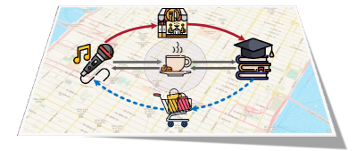
For introducing comparative learning into urban area embedding tasks, it is crucial to adopt appropriate data enhancement strategies for different data samples. However, existing enhancement methods, even those customized for sequential and spatio-temporal data, fail to meet the requirements. Two key reasons contribute to this limitation: (1) In the spatial dimension, each POI is discrete and highly semantic. Similarly, geographic neighborhood information is fixed in urban areas. Existing data augmentation methodsHou et al. (2022); He et al. (2020); Wei et al. (2019); Sun et al. (2020); Wang et al. (2021)such as replacement, masking, disruption, and cropping are insufficient to perturb POIs and neighbor sets to generate positive samples with a high degree of semantically similarity. (2) Each human mobility trip has distinct characteristics that make it easily distinguishable, which renders the corresponding contrastive pretext task being meaningless because the augmented samples are easily discriminated. As shown in Figure 1, replacing the POI of a mobility trip, such as a café, with a nearby restaurant or shopping mall, changes the semantics and purpose of the trip.
To tackle these challenges, we propose an urban region profiling model called EUPAS, which combines supervised and self-supervised learning to comprehend high-level semantics in noisy or incomplete urban data. Specifically, region heterogeneous graphs containing human mobility data, POIs information, and geographic neighborhood details for each region are fed into the model, which generates region embeddings that preserve intra-region and inter-region dependencies through GCNs and multi-head attention. Meanwhile, we introduce a spatial augmentation layer to generate positive samples that are semantically similar and spatially close to the anchor for subsequent contrastive learning. To enhance the contrastive learning effect, adversarial training is employed to generate ’hard’ negative samples through minor perturbations, minimizing semantic-level conditional likelihood. In contrast, ’strong’ positive samples result from larger perturbations while maintaining high conditional likelihood. This strategy ensures that negative samples are closely aligned with anchors in the latent embedding space, but are semantically different (e.g., travel purpose), while positive samples are farther away from the anchor, but are semantically similar. Finally, we jointly optimize supervised and self-supervised learning to facilitate the model in generating powerful region embeddings. In summary, our work has the following contributions:
-
•
To tackle the noise problem in urban data, we propose a joint supervised learning and self-supervised learning framework for urban region profiling.
-
•
To avoid tedious manual adjustments, we propose a spatial enhancement strategy to generate meaningful positive samples based on the specificity of urban region embedding for subsequent contrastive learning.
-
•
To further enhance contrastive learning, we employ an adversarial strategy to automatically generate hard positive-negative pairs, which encourages the model to comprehend the high-level semantics for the urban region embeddings.
-
•
We extensively evaluate our approach using real-world data through a series of experiments. The results demonstrate the superiority of our method compared to state-of-the-art baselines.
In the rest of this paper, we first present some preliminary definitions and define the problem. Then, we detail the proposed model and show the experimental settings and results. Finally, we conclude the paper.
2 Preliminaries
In this section, we first give some notations and define the urban region embedding problem. Suppose that a city is divided into a set of non-overlapping regions , where denotes the -th region and denotes the number of the regions.
Definition 1 (Human Mobility.).
Let represent a travel record, where is the origin region and is the target region with . Human mobility is defined as a set of trips occurring in urban areas, where is the number of trips.
Definition 2 (Regional POIs Information.).
Region function features are characterized by POIs in the city. We represent the region information as , where and is the number of categories.
Definition 3 (Geographic Neighbor Information.).
The geographical neighbor information signifies the spatial relationships between a region and its neighboring areas. Specifically, the set of geographical neighbors can be expressed as , where is the geographical neighbor vector for the urban region .
Definition 4 (Region heterogeneous graph.).
It is denoted as , where denotes the set of region nodes, with each node corresponding to a specific urban region. is the set of edges connecting the nodes, and represents the set of different edge types. Here, is the origin edge type, is the target edge type, is the POI edge type, and is the geographic neighbor edge type. and are constructed based on correlations of human mobility data, while is constructed using POI information. Regarding the edge type , we connect each node to all of its geographic neighbors.
Definition 5 (Urban Region Embedding.).
Given a set of regions , human mobility , POIs information , and geographical neighbor information , our goal is to learn low-dimensional embeddings , where represents the -dimensional embedding for the region . These embeddings in should capture movement patterns, geographic neighborhoods, and POI-related details for various urban downstream tasks.
3 Methodology
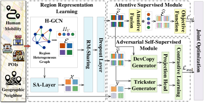
In this section, we present the technical details of our EUPAS framework. The overall model architecture is illustrated in Figure. 2, which mainly consists of three components, region representation learning, attentive supervised module, and adversarial self-supervised module.
3.1 Region Representation Learning
In this module, our focus is on leveraging the region heterogeneous graph to learn embeddings that capture multi-level urban features and inter-region semantic correlations. Simultaneously, we generate effective positive samples based on the acquired region embeddings in preparation for subsequent contrastive learning.
3.1.1 Heterogeneous GCN Layers (H-GCN)
To capture both intra-view and inter-view region dependencies, we conduct message passing on the heterogeneous region graph . Our model integrates relation embeddings into the GCN for enhanced graph learning. Let and denote the node and relation embeddings at the -th layer, respectively. Here, , , , and represent the relation embeddings for origin, target, POI, and geographic neighbor relationships, respectively. Then, given the initial node embedding and relation embedding , we update them at the layer as follows:
| (1) |
| (2) |
where , , and denotes a specific relation type. Here, represents the LeakyReLU activation function, and is the element-wise product. The learnable parameter for node embedding update in the -th layer is denoted as . Additionally, stands for the neighbor set of the region under relation type . To quantify the correlation between region vertex pair , we define the normalization weight , determined by the degrees of the vertices. Moreover, and are layer-specific parameters projecting relation embeddings from the previous layer to the same embedding space for subsequent use.
In addition, to mitigate feature smoothing in graph neural networks, we incorporate ResNetHe et al. (2016) into H-GCN for multi-layer graph aggregation. At the th layer, the aggregation process is expressed as follows:
| (3) |
where denotes the adjacency matrix, and is the corresponding diagonal matrix. To construct three adjacency matrices based on different data sources, for each node, we obtain the -nearest neighbors using various similarity matrices as its neighbors in the heterogeneous graph. Finally, we obtain the node embeddings and the relation embeddings under each relation type.
3.1.2 Relation-aware Message Sharing Layer (RM-Sharing)
Generally, different attributes within the same region are interrelated. For instance, factors like unemployment, poverty, and educational levels in neighboring areas may influence crime rates in certain regions. To capture global information, we employ the multi-head self-attention mechanismVaswani et al. (2017). Formally, given the relation-specific region embeddings set , we compute one-head self-attention as follows:
| (4) |
where , , and are learnable parameters for the -th head. We compute multi-head self-attention by the following equation:
| (5) |
where is the learnable parameter for transformation, denotes concatenation, and is the number of heads. Our model learns the region sharing embedding, denoted by . Subsequently, we introduce the learning-based linear interpolation to improve the embedding, formulated as follows:
| (6) |
where , , and denotes the learning parameters. Finally, we obtain the relation-aware region embedding, denoted by . To ensure the model’s generalization ability, dropout layers are further employed.
3.1.3 Spatial Augmentation Layer (SA-Layer)
To autonomously generate effective positive samples based on the specificity of urban region embeddings for subsequent contrastive learning preparation, we perturb the region embeddings in latent space. In particular, we use to denote the corresponding positive example. Formally,
| (7) |
where is sampled from a Gaussian distribution with zero mean and standard deviation . represents the scale factor for perturbation magnitude, with and serving as hyper-parameters. The result, denoted as , is then fed into RM-sharing to obtain spatial augmentation positive samples (SA-Pos), denoted as .
3.2 Attentive Supervised Module
In this section, we integrate relation-aware region sharing embeddings and an automatic learning weight coefficient to generate multi-task embeddings. The module utilizes a supervised learning loss function to optimize and ensure that learned region embeddings preserve region similarity across different attributes.
Given a relation-specific region sharing embedding , the attention coefficient is computed by averaging the weights of all node embeddings using shared parameters , , and :
| (8) |
where is the LeakyReLU activation function. The softmax function is then applied for normalization:
| (9) |
Continuing, utilizing the learned coefficients , we integrate the shared embeddings of four specific relations to obtain the region embeddings :
| (10) |
Finally, the learned region embedding and relation embedding are used to generate the multi-task embedding:
| (11) |
where , and denotes the element-wise product. The result is the final task embedding for downstream tasks.
To guide the model to learn meaningful and task-specific region representations, we define the supervised learning objective as:
| (12) |
where , , and are losses for geographic predictor, mobility predictor, and POI predictor respectively.
For the geographic predictor, designed to preserve neighborhood region properties, given the geographic embedding , we introduce the Triplet Margin Loss function:
| (13) |
where and are positive and negative samples of geographic neighbors, respectively.
Through the mobility predictor, we can predict the target (resp. origin) region when the origin (resp. target) region is provided. Given the mobility embeddings , and human mobility , we first compute original mobility distribution as follows:
| (14) |
We then reconstruct origin and target region distributions:
| (15) |
Hence, the mobility predictor loss, defined by Kullback-Leibler (KL) divergence, is:
| (16) |
The POI predictor aims to retain POI information in the final region representation. To achieve this, we follow the same approachZhang et al. (2020) to construct the POI similarity matrix . Given POI embedding , we have the POI loss formulated by:
| (17) |
3.3 Adversarial Self-Supervised Module
To avoid perturbations to the region embeddings producing positive samples with semantic biases, we employ adversarial perturbations for spatial augmentation to generate strong negative and positive pairs, which encourage our model to effectively capture the semantics of region embeddings and enjoy satisfactory generalization ability and robustness.
3.3.1 Adversarial Perturbations Layer
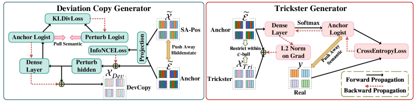
The studiesTian et al. (2020); Suresh et al. (2021) suggest stronger divergence and adversarial graph enhancements improve contrast learning. Taking into account the distinguishable characteristics of various region embeddings, hindering the efficacy of contrastive training, we advocate for the adoption of adversarial perturbations to generate hard negative and positive pairs. This strategy facilitates the meaningful extraction of high-level semantics within region embeddings, ensuring robust generalization. The Adversarial Perturbation Layer comprises the Trickster Generator and Deviation Copy Generator, with the detailed implementation processes depicted in Figure. 4.
The Trickster generator aims to produce hard negative samples, denoted as , that exhibit proximity to anchors in the latent embedding space while maintaining semantic distinctions. In particular, is derived by introducing a slight perturbation to the anchor , where the Euclidean norm of is constrained within the limit of . Simultaneously, in an effort to alter the inherent semantics as extensively as feasible, we aim to minimize the conditional likelihood of with respect to the real target denoted as . Formally,
| (18) |
where has the same size with . Due to the intractability of exact minimization for neural networks, we implement it as follows:
| (19) |
To address different types of region embeddings, we improve the Trickster generation by using various predictor losses (as detailed in Section 3.2) to generate perturbations.
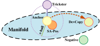
We introduce the deviation copy generator with the aim of generating an additional strong positive instance , referred to as DevCopy. It is intended to exhibit semantics similar to the anchor , while maintaining a far distance in the latent space. The relationship between them is illustrated in Figure 3. Specifically, a well-suited perturbation is introduced to to minimize its cosine similarity with . However, the exact computation of under these constraints is intractable. To address this, we use two computational phases to approximate it. In the first stage, a perturbation is added to to minimize the contrastive learning loss (refer to Eq.23, where can be viewed as and as ). Formally,
| (20) |
In the second step, we aim to maintain semantics by minimizing the KL divergence between the conditional likelihood and , pulling them closer together. Formally,In the second step, we aim to maintain semantics by minimizing the KL divergence between the conditional likelihood and , pulling them closer together. Formally,
| (21) |
| (22) |
Meanwhile, for comparative learning of heterogeneous graphs, we perform a linear projection Jiang et al. (2021) on and to be able to better estimate the mutual information.
| Dataset | Details |
|---|---|
| Regions | 180 regions based on the Manhattan community boards. |
| Taxi trips | 10 million taxicab trips during one month. |
| Check-in data | 100,000 check-in points with 200 categories. |
| POI data | 20,000 PoI in 13 categories in the studied areas. |
| Crime data | 40,000 criminal records in a year |
| Models | Check-in Prediction | Land Usage Classification | Crime Prediction | |||||
|---|---|---|---|---|---|---|---|---|
| MAE | RMSE | NMI | ARI | MAE | RMSE | |||
| LINE | 564.59 | 853.82 | 0.08 | 0.17 | 0.01 | 117.53 | 152.43 | 0.06 |
| node2vec | 372.83 | 609.47 | 0.44 | 0.58 | 0.35 | 75.09 | 104.97 | 0.49 |
| HDGE | 399.28 | 536.27 | 0.57 | 0.59 | 0.29 | 72.65 | 96.36 | 0.58 |
| ZE-Mob | 360.71 | 592.92 | 0.47 | 0.61 | 0.39 | 101.98 | 132.16 | 0.20 |
| MV-PN | 476.14 | 784.25 | 0.08 | 0.38 | 0.16 | 92.30 | 123.96 | 0.30 |
| CGAL | 315.58 | 524.98 | 0.59 | 0.69 | 0.45 | 69.59 | 93.49 | 0.60 |
| MVGRE | 297.72 | 495.27 | 0.63 | 0.78 | 0.59 | 65.16 | 88.19 | 0.64 |
| MGFN | 280.91 | 436.58 | 0.72 | 0.76 | 0.58 | 59.45 | 77.60 | 0.72 |
| ROMER | 252.14 | 413.96 | 0.74 | 0.81 | 0.68 | 64.47 | 85.46 | 0.72 |
| HREP | 270.28 | 406.53 | 0.75 | 0.80 | 0.65 | 65.66 | 84.59 | 0.68 |
| EUPAS(Ours) | 251.70 | 394.68 | 0.77 | 0.84 | 0.71 | 58.56 | 78.41 | 0.73 |
3.3.2 Contrastive Learning Layer
In the contrastive learning layer, we utilize the InfoNCE Loss to maximize the similarity between the anchor and DevCopy, while minimizing the similarity between the anchor and Trickster:
| (23) |
where measures the correlation between two embeddings, represents the spatially augmented positive sample (i.e., SA-Pos), and is a set of randomly selected negative samples from the same batch.
To enhance the contrastive learning process, we introduce ”hard” negative and positive examples. Firstly, we design the trickster contrastive loss by introducing the Trickster as an extra negative example:
| (24) |
where denotes .
To further enhance the training process, we introduce the strong positive sample :
| (25) |
In the end, the total contrastive loss is formulated as:
| (26) |
where is a hyper-parameter.
3.4 Joint Optimization
To jointly optimize the urban region profiling model, we combine the attentive supervised module and adversarial self-supervised learning, as follows,
| (27) |
where denotes the trainable parameters for regularization with the strength of . is a hyper-parameter.
4 Experiments
In our experimental study, we design three downstream applications to evaluate the performance of our model, including crime prediction, check-in prediction, and land usage classification. Our model is implemented with PyTorch on an NVIDIA RTX 3090 24G.

4.1 Datasets
Experiments are conducted on several real-world datasets from the Manhattan, New York area, accessible through the NYC Open Data website111https://opendata.cityofnewyork.us/. Human mobility is represented by taxi trip data. The Manhattan area is discretized into 180 regions corresponding to community boards. A detailed description of each dataset is provided in Table 1.
4.2 Experimental Settings
We optimize the model using Adam with a learning rate of 0.001. The model has a dimension of 144, and the heterogeneous GCN consists of 3 layers. In the multi-head self-attention, we use 4 heads. Hyperparameters are set as follows: = 0.01, = 1, = 1, = 0.50, = 0.15, and = 4. The epoch is set as 2000 in EUPAS.
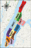
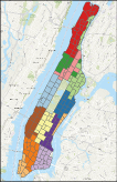
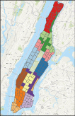
For land usage classification, our objective is to cluster regions with the same function using K-means. Community boards Berg (2007) divide Manhattan into 12 regions based on land use (shown in Figure 6(a)). Evaluation metrics include Normalized Mutual Information (NMI) and Adjusted Rand Index (ARI). Regression tasks (crime, check-in) use Mean Absolute Error (MAE), Root Mean Square Error (RMSE), and coefficient of determination () for evaluation.
4.3 Baselines
This paper compares the EUPAS model with state-of-the-art methods, categorized into three groups: (1) Traditional graph embedding methods, including LINETang et al. (2015) and node2vecGrover and Leskovec (2016); (2) Single data source methods, including HDGE Wang and Li (2017), ZE-MobYao et al. (2018), and MGFN Wu et al. (2022); (3) Multiple data source methods, including MV-PNFu et al. (2019), CGALZhang et al. (2019), MVGREZhang et al. (2020), ROMER Chan and Ren (2023), and HREP Zhou et al. (2023).
4.4 Experimental Results
4.4.1 Main Results
Table 2 summarizes the comparison results across all downstream tasks, with EUPAS emerging as the top performer, demonstrating the effectiveness of our combined supervised and adversarial self-supervised learning paradigm. Unlike EUPAS, traditional graph embedding methods such as LINE and node2vec fall short by being limited to learning node embeddings solely from the graph, missing the capacity to capture other regional information. Approaches leveraging human mobility data, including HDGE, ZE-Mob, CGAL, and MGFN, show significant improvements in downstream task performance. Furthermore, methods that incorporate diverse urban data sources, such as MVPN, MVGRE, HERP, and ROMER, outperform methods that focus on a single data type on average, highlighting the efficacy of multi-view fusion in integrating diverse relationships between regions. However, these approaches do not effectively address the challenge within the graph neural paradigm, where the noise effect intensifies during the message passing over the task-irrelevant region edges. In contrast, EUPAS introduces adversarial self-supervised signals to improve the learning of region representations against noise perturbations.
4.4.2 Ablation Study
To analyze the individual contributions of each component, we conduct an ablation study on three downstream tasks. Variants of EUPAS are designed as follows: (1) w/o Spatial Augmentation (w/o SA): Replacing the SA-layer with a replacement data augmentation approach to generate region embeddings positive samples for subsequent joint learning. (2) w/o supervised learning (w/o SL): Removing the attentive supervised module from EUPAS. (3) w/o self-supervised learning (w/o SSL): Removing the adversarial self-supervised module from EUPAS. (4) w/o Trickster (w/o T): Removing the from EUPAS, with the remaining settings identical to EUPAS. (5) w/o DevCopy (w/o D): Removing the from EUPAS, with the remaining settings identical to EUPAS.
Figure 5 illustrates the ablation results of EUPAS and its variants. The results show that an effective data augmentation approach is crucial for graph contrastive learning. Without the proposed spatial perturbation approach, the learning performance is inferior, emphasizing the significance of our spatially augmented perturbations in enhancing model robustness. Moreover, relying solely on self-supervised learning yields unsatisfactory results, highlighting the necessity of our joint framework of supervised and self-supervised learning. Additionally, the inclusion of Tickster and DevCopy further enhances the model’s discriminative performance, gradually increasing the difficulty of the augmented samples during training and strengthening the model’s discriminative ability. The optimal outcomes are achieved when all these modules are combined in our final model.
4.4.3 Visualized Analysis
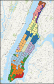
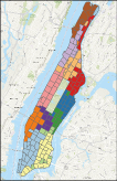
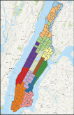
In Figure 6, we visually compare clustering results for land use classification among five baselines and our model. Regions sharing the same color belong to the same cluster. Remarkably, our model exhibits superior consistency with real ground conditions, indicating that it effectively represents regional functions by capturing high-level semantics in noisy urban data and extracting accurate urban region embeddings.
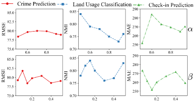
4.4.4 Hyperparameter Studies
We systematically tune important hyperparameters in EUPAS. The weighting parameter in Eq. 26 affects the sum of positive and negative sample losses in self-supervised learning, which we explored within , with =0.50 yielding the best performance. This balance turns out to be crucial for effective contrastive learning within our designed adversarial self-supervised module. For the joint optimization parameter in Eq. 27, varying within , the model excels with = 0.15, highlighting the dominant role of self-supervised learning in mining high-level region semantics from noisy urban data.
5 Conclusion
In this paper, we propose a pioneering method for urban region profiling by leveraging a combination of supervised and self-supervised learning paradigms. We employ graph adversarial self-supervised learning and devise a specialized pretext task to generate effective positive and negative samples for contrastive learning, overcoming the impact of data noise in region representation learning. Extensive experiments on real-world data validate the effectiveness and versatility of our proposed EUPAS in different settings.
Acknowledgments
This work was supported in part by the National Key RD Program of China under Grant No.2020YFB1710200, in part by the China Postdoctoral Science Foundation under Grant No.2022M711088, in part by the National Natural Science Foundation of China under Grant No.62172243.
References
- Berg [2007] Bruce F Berg. New York City Politics : Governing Gotham. Rutgers University Press, page 352, 2007.
- Chan and Ren [2023] Weiliang Chan and Qianqian Ren. Region-wise attentive multi-view representation learning for urban region embedding. In Proceedings of the 32nd ACM International Conference on Information and Knowledge Management, CIKM ’23, page 3763–3767, New York, NY, USA, 2023. Association for Computing Machinery.
- Chen et al. [2020] Ting Chen, Simon Kornblith, Mohammad Norouzi, and Geoffrey Hinton. A simple framework for contrastive learning of visual representations. In Proceedings of the 37th International Conference on Machine Learning, ICML’20. JMLR.org, 2020.
- Fu et al. [2019] Yanjie Fu, Pengyang Wang, Jiadi Du, Le Wu, and Xiaolin Li. Efficient Region Embedding with Multi-View Spatial Networks: A Perspective of Locality-Constrained Spatial Autocorrelations. Proceedings of the AAAI Conference on Artificial Intelligence, 33(01):906–913, July 2019.
- Grover and Leskovec [2016] Aditya Grover and Jure Leskovec. Node2vec: Scalable Feature Learning for Networks, July 2016.
- He et al. [2016] Kaiming He, Xiangyu Zhang, Shaoqing Ren, and Jian Sun. Deep residual learning for image recognition. In 2016 IEEE Conference on Computer Vision and Pattern Recognition (CVPR), pages 770–778, 2016.
- He et al. [2020] Kaiming He, Haoqi Fan, Yuxin Wu, Saining Xie, and Ross Girshick. Momentum contrast for unsupervised visual representation learning. In 2020 IEEE/CVF Conference on Computer Vision and Pattern Recognition (CVPR), pages 9726–9735, 2020.
- Hou et al. [2022] Zhenyu Hou, Xiao Liu, Yukuo Cen, Yuxiao Dong, Hongxia Yang, Chunjie Wang, and Jie Tang. Graphmae: Self-supervised masked graph autoencoders. In Proceedings of the 28th ACM SIGKDD Conference on Knowledge Discovery and Data Mining, KDD ’22, page 594–604, New York, NY, USA, 2022. Association for Computing Machinery.
- Huang et al. [2023] Weiming Huang, Daokun Zhang, Gengchen Mai, Xu Guo, and Lizhen Cui. Learning urban region representations with POIs and hierarchical graph infomax. ISPRS Journal of Photogrammetry and Remote Sensing, 196:134–145, February 2023.
- Jiang et al. [2021] Xunqiang Jiang, Tianrui Jia, Yuan Fang, Chuan Shi, Zhe Lin, and Hui Wang. Pre-training on large-scale heterogeneous graph. In Proceedings of the 27th ACM SIGKDD Conference on Knowledge Discovery & Data Mining, KDD ’21, page 756–766, New York, NY, USA, 2021. Association for Computing Machinery.
- Liu et al. [2019] Hao Liu, Ting Li, Renjun Hu, Yanjie Fu, Jingjing Gu, and Hui Xiong. Joint Representation Learning for Multi-Modal Transportation Recommendation. Proceedings of the AAAI Conference on Artificial Intelligence, 33(01):1036–1043, July 2019.
- Liu et al. [2023] Xiao Liu, Fanjin Zhang, Zhenyu Hou, Li Mian, Zhaoyu Wang, Jing Zhang, and Jie Tang. Self-supervised learning: Generative or contrastive. IEEE Transactions on Knowledge and Data Engineering, 35(1):857–876, 2023.
- Luo et al. [2022] Yan Luo, Fu-lai Chung, and Kai Chen. Urban region profiling via multi-graph representation learning. In Proceedings of the 31st ACM International Conference on Information & Knowledge Management, CIKM ’22, page 4294–4298, New York, NY, USA, 2022. Association for Computing Machinery.
- Rethmeier and Augenstein [2023] Nils Rethmeier and Isabelle Augenstein. A primer on contrastive pretraining in language processing: Methods, lessons learned, and perspectives. ACM Comput. Surv., 55(10), feb 2023.
- Sun et al. [2020] Fan-Yun Sun, Jordan Hoffmann, Vikas Verma, and Jian Tang. Infograph: Unsupervised and semi-supervised graph-level representation learning via mutual information maximization. In 8th International Conference on Learning Representations, ICLR 2020, Addis Ababa, Ethiopia, April 26-30, 2020. OpenReview.net, 2020.
- Suresh et al. [2021] Susheel Suresh, Pan Li, Cong Hao, and Jennifer Neville. Adversarial graph augmentation to improve graph contrastive learning. In M. Ranzato, A. Beygelzimer, Y. Dauphin, P.S. Liang, and J. Wortman Vaughan, editors, Advances in Neural Information Processing Systems, volume 34, pages 15920–15933. Curran Associates, Inc., 2021.
- Tang et al. [2015] Jian Tang, Meng Qu, Mingzhe Wang, Ming Zhang, Jun Yan, and Qiaozhu Mei. Line: Large-scale information network embedding. In Proceedings of the 24th International Conference on World Wide Web, WWW ’15, page 1067–1077, Republic and Canton of Geneva, CHE, 2015. International World Wide Web Conferences Steering Committee.
- Tian et al. [2020] Yonglong Tian, Chen Sun, Ben Poole, Dilip Krishnan, Cordelia Schmid, and Phillip Isola. What makes for good views for contrastive learning? In Proceedings of the 34th International Conference on Neural Information Processing Systems, NIPS’20, Red Hook, NY, USA, 2020. Curran Associates Inc.
- Vaswani et al. [2017] Ashish Vaswani, Noam Shazeer, Niki Parmar, Jakob Uszkoreit, Llion Jones, Aidan N. Gomez, Lukasz Kaiser, and Illia Polosukhin. Attention Is All You Need, December 2017.
- Wang and Li [2017] Hongjian Wang and Zhenhui Li. Region Representation Learning via Mobility Flow. In Proceedings of the 2017 ACM on Conference on Information and Knowledge Management, pages 237–246, Singapore Singapore, November 2017. ACM.
- Wang et al. [2021] Xiao Wang, Nian Liu, Hui Han, and Chuan Shi. Self-supervised heterogeneous graph neural network with co-contrastive learning. In Proceedings of the 27th ACM SIGKDD Conference on Knowledge Discovery & Data Mining, KDD ’21, page 1726–1736, New York, NY, USA, 2021. Association for Computing Machinery.
- Wang et al. [2022] Yuyang Wang, Jianren Wang, Zhonglin Cao, and Amir Barati Farimani. Molecular contrastive learning of representations via graph neural networks. Nat Mach Intell, 4(3):279–287, March 2022.
- Wei et al. [2019] Chen Wei, Lingxi Xie, Xutong Ren, Yingda Xia, Chi Su, Jiaying Liu, Qi Tian, and Alan L. Yuille. Iterative reorganization with weak spatial constraints: Solving arbitrary jigsaw puzzles for unsupervised representation learning. In 2019 IEEE/CVF Conference on Computer Vision and Pattern Recognition (CVPR), pages 1910–1919, 2019.
- Wu et al. [2022] Shangbin Wu, Xu Yan, Xiaoliang Fan, Shirui Pan, Shichao Zhu, Chuanpan Zheng, Ming Cheng, and Cheng Wang. Multi-Graph Fusion Networks for Urban Region Embedding, May 2022.
- Xie et al. [2023] Yaochen Xie, Zhao Xu, Jingtun Zhang, Zhengyang Wang, and Shuiwang Ji. Self-supervised learning of graph neural networks: A unified review. IEEE Transactions on Pattern Analysis and Machine Intelligence, 45(2):2412–2429, 2023.
- Yao et al. [2018] Zijun Yao, Yanjie Fu, Bin Liu, Wangsu Hu, and Hui Xiong. Representing Urban Functions through Zone Embedding with Human Mobility Patterns. In Proceedings of the Twenty-Seventh International Joint Conference on Artificial Intelligence, pages 3919–3925, Stockholm, Sweden, July 2018. International Joint Conferences on Artificial Intelligence Organization.
- You et al. [2020] Yuning You, Tianlong Chen, Yongduo Sui, Ting Chen, Zhangyang Wang, and Yang Shen. Graph contrastive learning with augmentations. In H. Larochelle, M. Ranzato, R. Hadsell, M.F. Balcan, and H. Lin, editors, Advances in Neural Information Processing Systems, volume 33, pages 5812–5823. Curran Associates, Inc., 2020.
- Zhang et al. [2017] Chao Zhang, Keyang Zhang, Quan Yuan, Haoruo Peng, Yu Zheng, Tim Hanratty, Shaowen Wang, and Jiawei Han. Regions, Periods, Activities: Uncovering Urban Dynamics via Cross-Modal Representation Learning. In Proceedings of the 26th International Conference on World Wide Web, pages 361–370, Perth Australia, April 2017. International World Wide Web Conferences Steering Committee.
- Zhang et al. [2019] Yunchao Zhang, Yanjie Fu, Pengyang Wang, Xiaolin Li, and Yu Zheng. Unifying Inter-region Autocorrelation and Intra-region Structures for Spatial Embedding via Collective Adversarial Learning. In Proceedings of the 25th ACM SIGKDD International Conference on Knowledge Discovery & Data Mining, pages 1700–1708, Anchorage AK USA, July 2019. ACM.
- Zhang et al. [2020] Mingyang Zhang, Tong Li, Yong Li, and Pan Hui. Multi-View Joint Graph Representation Learning for Urban Region Embedding. In Proceedings of the Twenty-Ninth International Joint Conference on Artificial Intelligence, pages 4431–4437, Yokohama, Japan, July 2020. International Joint Conferences on Artificial Intelligence Organization.
- Zhang et al. [2023] Qianru Zhang, Chao Huang, Lianghao Xia, Zheng Wang, Zhonghang Li, and Siuming Yiu. Automated spatio-temporal graph contrastive learning. In Proceedings of the ACM Web Conference 2023, WWW ’23, page 295–305, New York, NY, USA, 2023. Association for Computing Machinery.
- Zhou et al. [2023] Silin Zhou, Dan He, Lisi Chen, Shuo Shang, and Peng Han. Heterogeneous Region Embedding with Prompt Learning. AAAI, 37(4):4981–4989, June 2023.