Deformation dynamics of an oil droplet into a crescent shape during the intermittent motion

Abstract

A paraffin droplet containing camphor and oil red O dye floating on the water surface exhibits spontaneous motion with deformation by generating a surface tension gradient around the droplet. We focused on the intermittent motion with a pronounced deformation into a crescent shape observed at specific concentrations of camphor and oil red O. We quantitatively analyzed the time changes in the droplet deformation and investigated the role of the oil red O by measuring the time-dependent oil/water interfacial tension with the pendant drop method. The observed effect can be explained by adsorption of the oil red O molecules at the oil/water interface: the interfacial tension decreases gradually after the interface formation, resulting in the dynamic deformation of the droplet. The combination of the decrease in interfacial tension and the decrease in driving force related to camphor outflow generates intermittent motion with dynamic deformation into a crescent shape.

I Introduction

Self-propelled motion can be observed in many nonequilibrium systems, including living organisms. There are also nonliving systems in which the free energy is converted into mechanical motion. They are much less complex than living organisms, and the mechanism of their self-propulsion can be explained with mathematical models through physics and chemistry. Consequently, studies on nonliving self-propelled motion are crucial for deep understanding of the phenomenon on the grounds of nonequilibrium science.

A camphor disk placed on the water surface is one of the well-known examples of self-propelled particles[1, 2]. After a disk is placed on the water surface, a layer of camphor molecules is formed, reducing the surface tension. Fluctuations in the concentration gradient can appear around the disk, leading to the surface tension gradient that drives the disk toward the slightly lower concentration area. Once the disk starts moving, its motion is maintained since the surface tension is lower at the rear of the disk[3, 4, 5]. Thus, a circular camphor disk moves by spontaneously breaking symmetry[6, 7]. In typical laboratory conditions camphor molecules evaporate quickly; hence, the water surface tension recovers in a short time. Therefore, the stationary motion of a camphor disk can be observed for a long time exceeding one hour. The self-propulsion of a camphor disk has been studied for more than a century[8, 9]. While fluctuations govern the direction of motion of a circular camphor disk, the motion of an asymmetric disk is determined by its shape[10, 11, 12, 13, 14, 15, 16, 17]. For example, it has been shown both theoretically and experimentally that an elliptical object tends to move in the direction of its minor axis[16, 17]. There are also several systems in which the particle shape determines the motion[18, 19, 20, 21].

For the self-propelled motion of a solid object, its shape determines the motion, but the shape is not affected by the motion since it is fixed. On the contrary, the feedback between motion and shape can be anticipated for self-propelled soft objects like droplets because motion can modify the object shape, and the shape affects its motion. The interactions between motion and shape of self-propelled droplets were studied in a number of papers[22, 23, 24, 25, 26, 27, 28, 29, 30, 31, 32, 33, 34]. The relationship between shape and motion was also observed in biological systems. For example, a keratocyte cell moves with deformation, and it is known experimentally and theoretically that the direction of motion strongly correlates with its shape[35, 36]. Therefore, the mechanism of the coupling between motion and deformation is an important problem in self-propulsion in non-equilibrium systems. There have been several theoretical reports in which a generic model was constructed for the coupling between motion and deformation by considering the symmetric properties[37, 38, 39]. However, these studies are concerned with small magnitudes of deformation from a circle. As far as the authors know, there has been no universal description from the theoretical aspect that can be applied to large deformation.

It has been recently reported that a paraffin droplet with camphor floating on the water surface moves spontaneously. Such a droplet shows complex behavior that can be controlled by the concentration of the oil red O dye in the paraffin[40, 41]. For moderate oil red O concentrations, a droplet moves spontaneously with dynamic deformation, whose shape cannot be described by a perturbation from a circular shape. A quantitative analysis of the phenomenon should help us to better understand the self-propulsion for systems showing big shape deformation.

In the presented study, we investigated the mechanism of deformation of a paraffin droplet containing camphor and oil red O, in which intermittent motion with dynamic deformation can be observed depending on the concentrations of camphor and oil red O and the elapsed time from putting the droplet on the water surface. We mainly focused on the change between the crescent and circular shapes observed during the intermittent motion. We introduced the quantities that allow us to measure the degree of deformation and evaluated them by image processing of the experimental results. Then, we discussed the relationship between these quantities and the droplet speed. We also measured the interfacial tension between water and oil containing oil red O and proposed the deformation mechanism towards a crescent shape coupled with intermittent motion.

II Experimental Setup

II.1 Spontaneous motion of a droplet

(+)-Camphor and oil red O (dye) were purchased from FUJIFILM Wako Pure Chemical Corporation (Japan), and paraffin oil was purchased from Sigma-Aldrich (USA). The chemicals were used without further purification. Ion-free water was prepared with Elix UV3 (Merck, Germany). We prepared a paraffin solution of camphor and oil red O at different concentrations by stirring using a vortex mixer and sonication.

We observed the time evolution of a 20 $\mu$L droplet located on the water surface in a Petri dish with an inner diameter of 194.5 mm. The time evolution of the system was recorded from above for an hour at 50 fps with the CMOS camera (STC-MBS43U3V, OMRON SENTECH Co., LTD., Japan) equipped with the objective lens (3Z4S-LE SV-0814H, OMRON Co., LTD., Japan). The Petri dish was illuminated by a light panel placed below.

All experiments were performed at room temperature ($22\pm 2$^∘C). Analyses of the recorded videos were performed by an image-processing software ImageJ[42].

II.2 Interfacial tension between oil and water

The interfacial tension between pure water and oil was measured using the pendant drop method. Paraffin oil containing oil red O was ejected through a hook-shaped needle (4983 PD 22G, Kyowa Interface Science Co., Japan) into the aqueous phase. The droplet image was recorded from the side with the above-mentioned camera equipped with the objective lens (TEC-M55, CBC Co., Ltd., Japan). It was illuminated by the LED lamp (AS3000, AS ONE Co., Japan) located at the opposite side to the camera. The interfacial tension was calculated by fitting the shape of an oil droplet to a theoretical curve. The details are described in Appendix A.

III Results

III.1 Spontaneous motion of a droplet

A 20 $\mu$L droplet of paraffin oil with dissolved camphor (concentration 0.06 M) and oil red O (concentration 1.0 g/L) exhibited three different types of motion depending on the time $t$ elapsed from the moment when the droplet was placed on the water surface. At the beginning of the experiment, the droplet showed self-propelled motion along a straight line perturbed by reflections with the dish wall, as shown in Fig. 1(a-1). Approximately at $t=30$ s, the droplet began to rotate along the wall (Fig. 1(a-2)). Then, at $t\sim 2000$ s, the droplet motion switched to intermittent motion (Fig. 1(a-3)). At this stage, short intervals of time when a droplet moved (less than $10$ s) were separated by periods when it was standing. The droplet had a circular shape when it did not move, and it became elongated and exhibited deformation into a crescent shape during intermittent motion.

Figure 1: Typical long-time behavior of a paraffin droplet containing camphor (concentration 0.06 M) and oil red O (concentration 1.0 g/L) moving on a water surface. The time $t=0$ corresponds to the moment when the droplet was placed on the water surface. (a) Snapshots of the droplet motion at around $t\sim 0$ s (a-1), $t\sim 600$ s (a-2), and $t\sim 2100$ s (a-3). The superposed images of the droplet are shown with the time difference of 0.5 s (a-1) and 1.0 s (a-2, a-3). The red lines indicate the trajectories of the droplet center of mass (COM) position. (b) Droplet speed $v$ as a function of time $t$.

Hereafter, we focus on the intermittent motion shown in Fig. 1(a-3). We defined a single phase of intermittent motion based on the droplet speed as a function of time (cf. Fig. 3(b)). If the droplet stopped ($v\leq 2$ mm/s) for more than 4 s, then we assumed that the droplet was at the rest state. If the droplet at the rest state was accelerated and its speed overcame 10 mm/s, then we considered this moment as the start of the intermittent phase. In the case that the time duration between the start of motion and the return to the rest state was less than 10 s, we defined that the droplet had performed an intermittent motion, and we analyzed the time series during each intermittent motion in detail. To minimize the boundary effect we did not analyze the intermittent motion if the droplet got closer than 20 mm to the wall of the Petri dish. We also excluded the data after a fission.

In the following analysis, we focused on the correlations between the droplet speed and dynamic deformation into a crescent shape observed during the intermittent motion (Fig. 1(a-3)). The observed droplet elongation was always perpendicular to the direction of motion. To study the deformation dynamics quantitatively, we introduced the local coordinates associated with the direction of motion. Each frame of the observed time evolution was processed so that pixels representing the droplet were black (the logical value $1$) and all the others were white (the logical value $0$). For each frame, we calculated the droplet center $\bm{r}_{\mathrm{c}}(t)$ as the center of mass (COM) of the black pixels. The set of droplet centers defined the droplet trajectory. The origin of the local coordinate system was set at $\bm{r}_{\mathrm{c}}(t)$. The $Y$-axis was defined as parallel to a fitting line to the droplet trajectory with a least-square method and directed as the net displacement vector. The $X$-axis was set perpendicular to the $Y$-axis. Using these coordinates, we defined the time-dependent aspect ratio $R=a/b$, where $b$ is the width of the droplet measured on the $Y$-axis and $a$ is the length of the droplet projected on the $X$-axis as illustrated in Fig. 2(a). The second quantity describing time-dependent droplet shape is the front-back asymmetric parameter $A=\Delta\Sigma/(2\Sigma)$, where $\Sigma$ is the area (the number of black pixels) of the droplet image and $\Delta\Sigma$ is the area of the figure obtained by applying XOR operation to the original droplet image and its image reflected with respect to the $X$-axis as shown in Fig. 2(b). It should be noted that $0\leq A\leq 1$ and $A=0$ for a droplet with mirror symmetry on the $X$-axis.

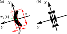
Figure 2: Illustration of parameters describing the droplet deformation. (a) Binarized image of a droplet. Aspect ratio is defined as $R=a/b$. (b) Image obtained by applying XOR operation to the droplet image and the image reflected to the $X$-axis. Asymmetric parameter $A$ is defined as the area of the image normalized by twice the area of the original image.

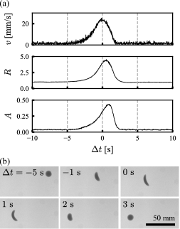
Figure 3: Dynamics of a single phase of the intermittent motion of a 20 $\mu$L paraffin droplet with camphor and oil red O. The concentrations of camphor and oil red O were 0.06 M and 1.0 g/L, respectively. (a) The speed $v$ of the droplet COM, the aspect ratio $R$, and the asymmetric parameter $A$ as functions of $\Delta t$. The time $\Delta t=0$ corresponds to when $v$ has the maximum value. (b) A sequence of frames showing droplet location and deformation during the phase of intermittent motion described in (a).

Figure 3(a) shows the speed $v(t)$ of the droplet center $(\bm{r}_{\mathrm{c}}(t))$ and the deformations $R(t)$ and $A(t)$ as functions of time during a single phase of intermittent motion illustrated in Fig. 3(b). The time $\Delta t=0$ corresponds to the moment when $v(t)$ has the maximum value. As shown in Fig. 3(a), the deformations began almost simultaneously when motion started. The speed $v(t)$ reached its maximum before the maxima of $R(t)$ and $A(t)$, which means that deformations still developed after the droplet started to slow down. This type of behavior was reproduced in many observations of intermittent motion, as shown in Fig. 4, in which the scatter plot of the time $\Delta t_{R}$ for the maximum of $R(t)$ and $\Delta t_{A}$ for the maximum of $A(t)$ is displayed. In almost all analyzed cases, both $\Delta t_{R}$ and $\Delta t_{A}$ were positive, and $\Delta t_{A}$ was slightly greater than $\Delta t_{R}$.

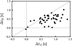
Figure 4: Scatter plot of $\Delta t_{A}$ and $\Delta t_{R}$, which are times for maximum values of $A(t)$ and $R(t)$ for the paraffin oil droplet with camphor and oil red O. The camphor concentration was 0.06 M and oil red O concentration was 1.0 g/L.

Next, we investigated the dependence of the droplet deformation on the oil red O concentration. We performed experiments at oil red O concentrations in the range of 0.5–1.1 g/L. The maximum values of $R(t)$ and $A(t)$ ($R_{\mathrm{max}}$ and $A_{\mathrm{max}}$), increased for oil red O concentrations larger than approximately 0.7 g/L as shown in Fig. 5.

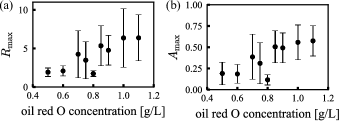
Figure 5: (a) Maximum values of $R_{\mathrm{max}}$ and (b) $A_{\mathrm{max}}$, for $R(t)$ and $A(t)$ as functions of oil red O concentration. The camphor concentration was 0.06 M, and experiments at each oil red O concentration were repeated more than 5 times. The error bars indicate the standard deviation of the results.

III.2 Interfacial tension between oil and water

To understand the role of oil red O, we measured the interfacial tension $\gamma_{\mathrm{ow}}(t)$ between the paraffin droplet containing oil red O and pure water using the pendant drop method[43] as a function of time. The measurement was performed for various oil red O concentrations. The interfacial tension gradually decreased in time after the interface was formed in the case that the oil red O concentration was higher, as shown in Fig. 6. For quantitative evaluation, we fitted time-dependent interfacial tension $\gamma_{\mathrm{ow}}(t)$ to an exponential function

$$\gamma_{\mathrm{ow}}(t)=\gamma_{\mathrm{ow}}^{(0)}-\Delta\gamma_{\mathrm{ow}}(1-e^{-t/\tau}),$$ (1)

where $\gamma_{\mathrm{ow}}^{(0)}$ is the interfacial tension at the initial stage, $\Delta\gamma_{\mathrm{ow}}$ is the difference in interfacial tension between the initial and final stages, and $\tau$ is the characteristic time for the decrease in interfacial tension. We plotted $\gamma_{\mathrm{ow}}^{(0)}$, $\Delta\gamma_{\mathrm{ow}}$ and $\tau$ against oil red O concentration in Fig. 7. $\gamma_{\mathrm{ow}}^{(0)}$ and $\Delta\gamma_{\mathrm{ow}}$ were decreasing and increasing functions of oil red O concentration, respectively. In the case when the decrease in interfacial tension was clearly observed (oil red O concentrations: 0.5, 0.8, and 1.0 g/L), $\tau$ was approximately 800 s. In addition, we performed the same measurement for the oil droplet that contained both oil red O (1.0 g/L) and camphor (0.06 M). The decrease in interfacial tension was also observed, and $\gamma_{\mathrm{ow}}^{(0)}$ was lower compared to that for the oil droplet with oil red O (1.0 g/L) but without camphor.

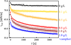
Figure 6: Time evolution of the interfacial tension $\gamma_{\mathrm{ow}}(t)$ between water and paraffin oil droplet measured by the pendant drop method. The time $t=0$ corresponds to when a droplet was formed. Curve colors correspond to oil red O concentrations: 0 g/L black, 0.1 g/L yellow, 0.5 g/L orange, 0.8 g/L red, 1.0 g/L dark red. The average values of four experiments are plotted. The error bars indicate the standard deviation of the results. $\gamma_{\mathrm{ow}}(t)$ between pure water and paraffin oil droplet that contained both oil red O (1.0 g/L) and camphor (0.06 M) is plotted as blue squares.

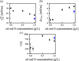
Figure 7: Parameters fitting $\gamma_{\mathrm{ow}}(t)$ according to Eq. 1 for different concentrations of oil red O (cf. Fig. 6). (a) Interfacial tension on the initial stage $\gamma_{\mathrm{ow}}^{(0)}$. (b) Difference in interfacial tension $\Delta\gamma_{\mathrm{ow}}$ between the initial and final stages. (c) Characteristic time $\tau$ for the decrease in interfacial tension. The data for a paraffin oil droplet that contained both oil red O (1.0 g/L) and camphor (0.06 M) are shown with blue squares. The average values for four measurements are shown. The error bars indicate their standard deviations.

IV Discussion

IV.1 Quantitative model for droplet deformation

The motion and deformation of a droplet are attributed to the surface tension difference induced by camphor molecules. However, a large deformation of a droplet shape without fission has not been observed without oil red O[40]. This suggests that the presence of oil red O molecules decreases the interfacial tension between water and oil, and this enables a large deformation. As illustrated in Figs. 6 and 7, the equilibration of the oil/water interface in the presence of oil red O molecules is slow since the characteristic time for the decrease in interfacial tension is around 800 s. Moreover, the camphor concentration in the droplet decreases over time. As a result, the gradient of interfacial tension around the droplet gets smaller in time, and the character of motion changes from translational to intermittent with dynamic deformation into a crescent shape.

Now, let us present quantitative arguments on how the decrease in interfacial tension induced deformation by evaluating the energy of deformation. If we neglect the contribution of the periphery, then the free energy of a floating droplet shown in Fig. 8 is estimated as:

$$F=-S\Sigma+\frac{1}{2}\left(\Delta\rho_{\mathrm{ao}}e_{\mathrm{ao}}^{2}+\Delta\rho_{\mathrm{ow}}e_{\mathrm{ow}}^{2}\right)g\Sigma,$$ (2)

Here, $S=\gamma_{\mathrm{aw}}-(\gamma_{\mathrm{ow}}+\gamma_{\mathrm{ao}})$ is the spreading coefficient, $\gamma_{\mathrm{aw}},\gamma_{\mathrm{ow}}$ and $\gamma_{\mathrm{ao}}$ are the interfacial tensions between air and water, oil and water, and air and oil, respectively, $\Sigma$ is the area of the droplet, and $\Delta\rho_{\mathrm{ao}}$ and $\Delta\rho_{\mathrm{ow}}$ are the density differences between air and oil and that between oil and water, respectively, as shown in Fig. 8. $e_{\mathrm{ao}}$ and $e_{\mathrm{ow}}$ are the differences in height between the water level at infinity and the air/oil interface, and that between the water level at infinity and the oil/water interface, respectively. We neglected the second term as it is much smaller than the first term since the thickness of the droplet is small.

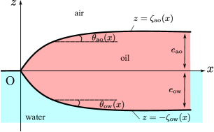
Figure 8: Schematic illustration of an oil droplet floating on the water surface. The triple line matches $x=z=0$. The functions $z=\zeta_{\mathrm{ao}}(x)$ and $z=-\zeta_{\mathrm{ow}}(x)$ indicate the interface between air and oil and that between oil and water, respectively. $\theta_{\mathrm{ao}}(x)$ and $\theta_{\mathrm{ow}}(x)$ are the slopes of them, i.e., $\tan\theta_{\mathrm{ao}}(x)=\mathrm{d}\zeta_{\mathrm{ao}}/\mathrm{d}x$ and $\tan\theta_{\mathrm{ow}}(x)=\mathrm{d}\zeta_{\mathrm{ow}}/\mathrm{d}x$. $e_{\mathrm{ao}}$ and $e_{\mathrm{ow}}$ are the differences in height between the water level at infinity and the air/oil interface, and that between the water level at infinity and the oil/water interface, respectively.

Additionally, a droplet should have excess energy since its periphery is curved. The excess energy per unit periphery length equals

$$\mathcal{T}= \frac{4}{3}\gamma_{\mathrm{ao}}\kappa_{\mathrm{ao}}^{-1}\left(1-\cos^{2}\frac{\theta_{\mathrm{ao}}(x=0)}{2}\right)$$ (3)

$$+\frac{4}{3}\gamma_{\mathrm{ow}}\kappa_{\mathrm{ow}}^{-1}\left(1-\cos^{2}\frac{\theta_{\mathrm{ow}}(x=0)}{2}\right),$$

where $\kappa_{\mathrm{ao}}^{-1}$ and $\kappa_{\mathrm{ow}}^{-1}$ are capillary lengths of air/oil and oil/water interfaces, respectively. $\theta_{\mathrm{ao}}(x=0)$ is the angle between the air/oil interface and the $x$-axis, and $\theta_{\mathrm{ow}}(x=0)$ is that between the oil/water interface and the $x$-axis. These values can be calculated from the balance at the triple line. That is, by assuming the water surface outside of the droplet is completely flat, we obtain

$$\cos\theta_{\mathrm{ao}}(x=0) =\frac{\gamma_{\mathrm{aw}}^{2}-\gamma_{\mathrm{ow}}^{2}+\gamma_{\mathrm{ao}}^{2}}{2\gamma_{\mathrm{aw}}\gamma_{\mathrm{ao}}},$$ (4)

$$\cos\theta_{\mathrm{ow}}(x=0) =\frac{\gamma_{\mathrm{aw}}^{2}-\gamma_{\mathrm{ao}}^{2}+\gamma_{\mathrm{ow}}^{2}}{2\gamma_{\mathrm{aw}}\gamma_{\mathrm{ow}}}.$$ (5)

The detail in the derivation is in Appendix B. The free energy of droplet deformation is described as:

$$\Delta E=\Delta E_{\Sigma}+\Delta E_{l},$$ (6)

where $\Delta E_{\Sigma}=-S\Delta\Sigma$ is the energy for an increase in droplet area $\Delta\Sigma$, and $\Delta E_{l}=\mathcal{T}\Delta l$ is energy for an increase in droplet periphery $\Delta l$. If the surface tension difference between the front and back of the droplet is $\delta\gamma_{\mathrm{aw}}$ and the droplet swept a water surface with an area of $\sigma$, then the work exerted on the droplet is estimated as

$$W=\delta\gamma_{\mathrm{aw}}\sigma.$$ (7)

We believe $\delta\gamma_{\mathrm{aw}}$ is no larger than 0.3 mN/m from the quasi-elastic laser scattering (QELS) measurement shown in Appendix C, though we could not measure the value directly. We used $\delta\gamma_{\mathrm{aw}}=0.24$ mN/m for the following calculation. For the intermittent motion shown in Fig. 3, we got $\Delta\Sigma=3.3$ mm², $\Delta l=17.2$ mm and $\sigma=1288.5$ mm². For these parameters and measured values of interfacial tensions by Wilhelmy method, $\gamma_{\mathrm{ao}}=31.6$ mN/m and $\gamma_{\mathrm{aw}}=73.5$ mN/m, the values of $\Delta E_{\Sigma},\Delta E_{l}$ and $W$ are plotted against $\gamma_{\mathrm{ow}}$ in Fig. 9(a). For these realistic values of parameters ($\gamma_{\mathrm{ow}}\sim 50$ mN/m), $\Delta E_{\Sigma}+\Delta E_{l}$ and $W$ are on the same order, which implies the deformation of the droplet is possible. $\Delta E_{\Sigma}$ and $\Delta E_{l}$ increase with an increase in interfacial tension $\gamma_{\mathrm{ow}}$ while $W$ does not depend on $\gamma_{\mathrm{ow}}$. In particular, the dependence of $\Delta E_{l}$ is greater than that of $\Delta E_{\Sigma}$. Figure 9(b) shows the energy of deformation normalized by the work exerted on the droplet. The droplet is expected to change spontaneously its shape if $\Delta E/W$ is smaller than one. On the contrary, a spontaneous dynamic droplet deformation is not possible when the interfacial tension is high because $\Delta E/W$ is greater than one. Thus in our experiment, the droplet can deform in the late stage since the oil/water interfacial tension decreased in time.

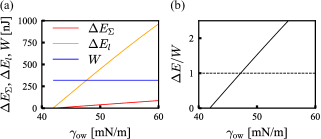
Figure 9: Dependence of energy of deformation on the interfacial tension between oil and water. (a) Plots of $\Delta E_{\Sigma}$ (red), $\Delta E_{l}$ (orange) and $W$ (blue), respectively. (b) Energy of deformation normalized by the work exerted on the droplet, $\Delta E/W$ against $\gamma_{\mathrm{ow}}$.

IV.2 Deformation of a droplet with oil red O

The time evolution of the interfacial tension shown in Fig. 6 and the discussion in the energy of deformation in the previous subsection indicate that the droplet deformation becomes easier with time $t$ after it was placed on the water surface. To confirm this, we investigated the deformation of a camphor-free droplet with oil red O by touching a camphor disk to the water surface close to the droplet. We put a 20 $\mu$L droplet of paraffin oil with oil red O (concentration 1.0 g/L) and without camphor on the water surface. Then, after time $T$, we touched a 3 mm-diameter camphor disk to the water surface at around 5 mm from the periphery of the droplet. Then, the droplet escaped from the camphor disk with deformation into a crescent shape as shown in Fig. 10(a). We performed experiments for $T=180,300,600$ s and plotted the characteristic parameters describing the droplet shape dynamics in Fig. 10(b), which are defined in the same manner as in Sec. III. The time $\Delta T=0$ corresponds to when the droplet COM speed $v$ has the maximum value. The maximum magnitude of deformation $A_{\mathrm{max}}$ increased with $T$ as shown in Fig. 10(b-2). The shape of the droplet was greatly curved when $T=600$ s, which should be the reason why $R_{\mathrm{max}}$ was smaller than that when $T=300$ s. Figure 10(b-3) shows a scatter plot of the times $\Delta T_{R}$ and $\Delta T_{A}$, at which the maximum values of $R$ and $A$ ($R_{\mathrm{max}}$ and $A_{\mathrm{max}}$) were observed. Both $\Delta T_{R}$ and $\Delta T_{A}$ were positive and had almost the same value. These behaviors were the same as those for the spontaneous deformation of a droplet with camphor shown in Fig. 4, though the relationship between $\Delta T_{R}$ and $\Delta T_{A}$ was slightly different from that between $\Delta t_{R}$ and $\Delta t_{A}$. This may be due to the much larger deformation in the experiments with a camphor-free droplet. When $T=30$ s, the droplet hardly deformed as shown in Fig. 10(c). The result in Fig. 10 shows that for longer $T$ droplet deformation becomes easier.

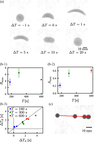
Figure 10: Deformation of a droplet (oil red O concentration 1.0 g/L) observed when the water surface was touched with a camphor disk after elapsed time $T$ since the droplet had been placed on the water surface. The time $\Delta T=0$ corresponds to when $v$ has the maximum value. (a) Snapshots of a droplet for $T=300$ s. (b) The characteristic values for the droplet deformation. (b-1) and (b-2) show the average value for $R_{\mathrm{max}}$ and $A_{\mathrm{max}}$ with the standard deviation as error bars for 3 experiments for each $T$, and (b-3) is a scatter plot of $\Delta T_{A}$ and $\Delta T_{R}$. (c) Superposed images of a droplet for $T=30$ s with a time difference of 2.0 s. The red line indicates the trajectories of the droplet COM.

V Conclusions

A paraffin droplet containing camphor and oil red O dye exhibits spontaneous motion with deformation. At considered concentrations of camphor and oil red O, the droplet started to perform intermittent motion approximately 2000 s after placing it on the water surface. In the presented study, we introduced a quantitative model that describes the possibility of large deformation of a droplet during intermittent motion. The model predicts that the shape deformation occurs when the oil/water interfacial tension becomes lower. It can spontaneously happen for a droplet located on the water surface because, after the formation of the interface, oil/water interfacial tension gradually decreases in time due to the adsorption of oil red O at the oil/water interface. Simultaneously, the camphor concentration in the droplet also decreases with time, resulting in a smaller driving force. The combination of decreased interfacial tension due to oil red O and reduced driving force due to reduced camphor concentration in the droplet causes intermittent motion with dynamic deformation into a crescent shape.

Appendix A Pendant drop method

A.1 Shape of a droplet

Let us consider a droplet formed above the tip of a needle as shown in Fig. 11 since the density of the droplet is lower than that of the bulk. We set the Cartesian coordinates so that the $z$-axis corresponds to the center axis of the needle as shown in Fig. 11(a). The top point of the droplet is set to be the origin, and the direction of $z$ is set downward. We assume the shape of the droplet is symmetric with respect to the $z$-axis. Due to the symmetry, we only consider the droplet profile on the $xz$-plane.

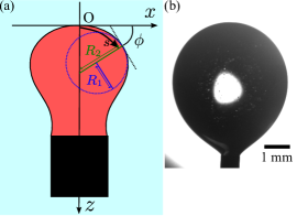
Figure 11: Shape of the oil droplet on the tip of a needle. (a) Schematic illustration of the coordinate system used to describe a droplet. The red and cyan areas represent the oil and water phases, and the black marks the needle tip. The blue line marks the curvature radius $R_{1}$ in the $xz$-plane, and the green one marks the curvature radius $R_{2}$ in the plane perpendicular to the $xz$-plane. (b) The droplet image obtained in the experiment for the measurement with the pendant drop method.

The balance between Laplace pressure and hydrostatic pressure yields

$$\left(\frac{1}{R_{1}}+\frac{\sin\phi}{x}\right)\gamma=p_{0}-\rho gz$$ (8)

at every point on the outline of the droplet except for the origin, where $R_{1}$ is a radius of curvature in the $xz$-plane, $\phi$ is an angle between the tangent line of the curve and the $x$-axis, $p_{0}$ is the hydrostatic pressure at the origin, and $\rho$ is a difference in density between the droplet and bulk. At the origin, the relation

$$\frac{2\gamma}{b}=p_{0}$$ (9)

is satisfied, where $b$ is the radius of curvature at the origin. Eliminating $p_{0}$ from Eqs. (8) and (9), we get

$$\frac{1}{R_{1}}+\frac{\sin\phi}{x}=\frac{2}{b}-\frac{\rho g}{\gamma}z.$$ (10)

By introducing the length $s$ along the curve from the origin, we obtain

$$\frac{\mathrm{d}\phi}{\mathrm{d}s}=\frac{1}{R_{1}}=\frac{2}{b}-\beta z-\frac{\sin\phi}{x},$$ (11)

$$\frac{\mathrm{d}x}{\mathrm{d}s}=\cos\phi,$$ (12)

$$\frac{\mathrm{d}z}{\mathrm{d}s}=\sin\phi,$$ (13)

where $\beta=\rho g/\gamma$. The shape of the droplet can be calculated by integrating Eqs. (11)–(13) by $s$ from $s=0$, where $\phi=0$ at $s=0$. By comparing the calculated curve with the image recorded in the experiments we obtained $b$, $\beta$, and thus,the interfacial tension $\gamma$ using $\gamma=\rho g/\beta$.

A.2 Analysis method

We recorded a sequence of droplet images every 60 s and calculated the interfacial tension for each image in the experiments. The droplet shape is described in the reference frame illustrated in Fig. 11(a). The vertical direction of images obtained in an experiment can differ from the actual vertical direction since the camera can be set at a slightly rotated angle. To compensate for the effect, we rotated the images with an angle $\theta$. For appropriate $\theta$, the shape of the droplet should be symmetric with respect to the vertical line. To find such an angle, the value of:

$$E_{\theta}=\sum_{z}\left(X_{r}(z,\theta)+X_{l}(z,\theta)\right)^{2}$$ (14)

was minimized. Here, $X_{r}(z,\theta)$ $(>0)$ and $X_{l}(z,\theta)$ $(<0)$ are the $x$ coordinates of the right and left peripheries at height $z$ for the rotated image. Since the position of the camera was fixed, $\theta$ should be identical for all the images of the sequence. Thus, we adopted the average of $\theta$ obtained by minimizing $E_{\theta}$ using the data of extracted 10 images. Hereafter, we use the rotated image, and the top point of the droplet estimated from the image is set to be the origin.

Next, the transformed data are compared with numerical results obtained from Eqs. (11)–(13). This calculation yields a set of coordinates $(x_{i},z_{i})$ along the edge of the droplet depending on the parameters $b$ and $\beta$. They also depend on the boundary values $x_{\mathrm{tp}}$ and $z_{\mathrm{tp}}$, which correspond to the coordinates of the top point.

Then, we compared the calculated coordinates at the droplet periphery $(x_{i},z_{i})$ and that obtained by the experiments $(X_{j},Z_{j})$. For the points $(X_{j},Z_{j})$ close to the origin, i.e., $\phi<\pi/4$, we compared the value of $z$ for each $x$. For the points $(X_{i},Z_{i})$ below them, i.e., $\phi>\pi/4$, we compared the value of $x$ for each $z$. Since the error in the region close to the needle should be large, we excluded the data where the width of the droplet was less than 1.5 times of the thickness of the needle. Then, we minimized

$$E(\beta,b,x_{\mathrm{tp}},z_{\mathrm{tp}})= \sum_{i}\left(X_{i}-x_{i}-x_{\mathrm{tp}}\right)^{2}$$

$$+\sum_{j}\left(Z_{j}-z_{j}-z_{\mathrm{tp}}\right)^{2},$$ (15)

with respect to $b$, $\beta$, $x_{\mathrm{tp}}$ and $z_{\mathrm{tp}}$. The top point of the droplet ($x_{\mathrm{tp}}$, $z_{\mathrm{tp}}$) should roughly match the origin, though it can differ because of the finite size of the pixel. $x_{\mathrm{tp}}$ and $z_{\mathrm{tp}}$ are introduced to compensate this effect. From the value of $\beta$, we get $\gamma_{\mathrm{ow}}$. It should be noted that the initial values for the parameters to minimize $E(\beta,b,x_{\mathrm{tp}},z_{\mathrm{tp}})$ are determined as follows; For the first image ($t=0$), we estimate the interfacial tension $\gamma_{0}$ from the maximum width $D$ of the droplet, and the width $d$ at $z=D$ using $d/D$ method[43] and adopt $\beta=\rho g/\gamma_{0}$, $b=D/2$ and $x_{\mathrm{tp}}=z_{\mathrm{tp}}=0$ as the initial values of the parameters. For the second or later image, we use the values of $\beta$, $b$, $x_{\mathrm{tp}}$, and $z_{\mathrm{tp}}$ that minimize $E(\beta,b,x_{\mathrm{tp}},z_{\mathrm{tp}})$ in the previous image as the initial values to accelerate the calculation.

Appendix B Derivation of the equation for line tension

Assuming the characteristic length of deformation of a triple line is much larger than the capillary length, we consider the deformation of the interface near the straight triple line. We set the Cartesian coordinates so that the $y$-axis matches the triple line and $z=\zeta_{\mathrm{ao}}(x)(x>0)$ and $z=\zeta_{\mathrm{ow}}(x)(x>0)$ indicate the interface between air and oil and that between oil and water, respectively, as shown in Fig. 9. Then, the excess energy of the triple line per unit length is described as

$$\mathcal{T}=\mathcal{T}_{\mathrm{ao}}+\mathcal{T}_{\mathrm{ow}},$$ (16)

where $\mathcal{T}_{\mathrm{ao}}$ and $\mathcal{T}_{\mathrm{ow}}$ originate from the air/oil and oil/water interfaces, respectively, and they are explicitly estimated as[44]

$$\mathcal{T}_{\mathrm{ao}}= \int_{0}^{\infty}\mathrm{d}x\biggr{\{}\gamma_{\mathrm{ao}}\left(\frac{1}{\cos\theta_{\mathrm{ao}}(x)}-1\right)$$

$$\qquad+\frac{1}{2}\rho_{\mathrm{ao}}g(e_{\mathrm{ao}}-\zeta_{\mathrm{ao}}(x))^{2}\biggr{\}},$$ (17)

$$\mathcal{T}_{\mathrm{ow}}= \int_{0}^{\infty}\mathrm{d}x\biggr{\{}\gamma_{\mathrm{ow}}\left(\frac{1}{\cos\theta_{\mathrm{ow}}(x)}-1\right)$$

$$+\qquad\frac{1}{2}\rho_{\mathrm{ow}}g(e_{\mathrm{ow}}-\zeta_{\mathrm{ow}}(x))^{2}\biggr{\}},$$ (18)

where $\tan\theta_{\mathrm{ao}}(x)=\mathrm{d}\zeta_{\mathrm{ao}}/\mathrm{d}x$ and $\tan\theta_{\mathrm{ow}}(x)=\mathrm{d}\zeta_{\mathrm{ow}}/\mathrm{d}x$. The shape of the droplet $\zeta_{\mathrm{ao}}(x)$ and $\zeta_{\mathrm{ow}}(x)$ can be calculated by minimizing $\mathcal{T}_{\mathrm{ao}}$ and $\mathcal{T}_{\mathrm{ow}}$ with respect to $\zeta_{\mathrm{ao}}$ and $\zeta_{\mathrm{ow}}$. Then, we get

$$-\gamma_{\mathrm{ao}}\cos^{3}\theta_{\mathrm{ao}}(x)\frac{\mathrm{d}^{2}\zeta_{\mathrm{ao}}}{\mathrm{d}x^{2}}=\rho_{\mathrm{ao}}g(e_{\mathrm{ao}}-\zeta_{\mathrm{ao}}(x)),$$ (19)

$$-\gamma_{\mathrm{ow}}\cos^{3}\theta_{\mathrm{ow}}(x)\frac{\mathrm{d}^{2}\zeta_{\mathrm{ow}}}{\mathrm{d}x^{2}}=\rho_{\mathrm{ow}}g(e_{\mathrm{ow}}-\zeta_{\mathrm{ow}}(x)),$$ (20)

which lead

$$\mathcal{T}_{\mathrm{ao}}=\frac{4}{3}\gamma_{\mathrm{ao}}\kappa_{\mathrm{ao}}^{-1}\left(1-\cos^{2}\frac{\theta_{\mathrm{ao}}(x=0)}{2}\right),$$ (21)

$$\mathcal{T}_{\mathrm{ow}}=\frac{4}{3}\gamma_{\mathrm{ow}}\kappa_{\mathrm{ow}}^{-1}\left(1-\cos^{2}\frac{\theta_{\mathrm{ow}}(x=0)}{2}\right),$$ (22)

where $\kappa_{\mathrm{ao}}^{-1}$ and $\kappa_{\mathrm{ow}}^{-1}$ are capillary lengths of air/oil and oil/water interfaces, respectively. From these equations, we can derive Eq. (3).

Appendix C Water surface tension measurement around a droplet

We measured the surface tension around a 30 $\mu$L paraffin droplet with camphor (concentration 0.06 M) and oil red O (concentration 1.0 g/L) using quasi-elastic laser scattering (QELS) method[5]. We put a metal screw on the bottom of the Petri dish upside down and then placed a droplet on the tip of the screw so that the droplet was pinned. We measured the surface tension close to the spot where the droplet was pinned. The optical settings for the surface tension measurement were the same as described in [5].

The decrease in surface tension $\gamma_{\mathrm{aw}}-\gamma_{\mathrm{aw}}^{(0)}$ is plotted as a function of time $t$ in Fig. 12, in which the initial value $\gamma_{\mathrm{aw}}^{(0)}$ is determined by fitting the time series for $0~{}\mathrm{s}\leq t\leq 40~{}\mathrm{s}$ to an exponential function

$$\gamma_{\mathrm{aw}}(t)=\gamma_{\mathrm{aw}}^{(0)}-\Delta\gamma_{\mathrm{aw}}(1-e^{-t/\tau}).$$ (23)

Time $t=0$ corresponds to the time when the droplet was placed on the tip of the screw. The surface tension slightly decreased by $\Delta\gamma_{\mathrm{aw}}=0.24$ mN/m.

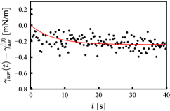
Figure 12: Decrease in the surface tension depending on time $t$ after putting a droplet on the water surface. The red line shows the exponential function obtained by the fitting with Eq. (23). The paraffin droplet included camphor at 0.06 M and oil red O at 1.0 g/L.

References

- Nakata et al. [2018] S. Nakata, V. Pimienta, I. Lagzi, H. Kitahata, and N. J. Suematsu, Self-organized Motion: Physicochemical Design based on Nonlinear Dynamics (The Royal Society of Chemistry, 2018).
- Nakata et al. [2015] S. Nakata, M. Nagayama, H. Kitahata, N. J. Suematsu, and T. Hasegawa, Phys. Chem. Chem. Phys. 17, 10326 (2015).
- Karasawa et al. [2018] Y. Karasawa, T. Nomoto, L. Chiari, T. Toyota, and M. Fujinami, J. Colloid Interface Sci. 511, 184 (2018).
- Karasawa et al. [2014] Y. Karasawa, S. Oshima, T. Nomoto, T. Toyota, and M. Fujinami, Chem. Lett. 43, 1002 (2014).
- Nomoto et al. [2023] T. Nomoto, M. Marumo, L. Chiari, T. Toyota, and M. Fujinami, J. Phys. Chem. B 127, 2863 (2023).
- Nagayama et al. [2004] M. Nagayama, S. Nakata, Y. Doi, and Y. Hayashima, Physica D: Nonlinear Phenomena 194, 151 (2004).
- Hayashima et al. [2001] Y. Hayashima, M. Nagayama, and S. Nakata, J. Phys. Chem. B 105, 5353 (2001).
- Tomlinson and Miller [1862] C. Tomlinson and W. A. Miller, Proc. R. Soc. London 11, 575 (1862).
- Strutt [1890] R. J. Strutt, Proc. R. Soc. London 47, 364 (1890).
- Nakata et al. [1997] S. Nakata, Y. Iguchi, S. Ose, M. Kuboyama, T. Ishii, and K. Yoshikawa, Langmuir 13, 4454 (1997).
- Boniface et al. [2019] D. Boniface, C. Cottin-Bizonne, R. Kervil, C. Ybert, and F. Detcheverry, Phys. Rev. E 99, 062605 (2019).
- Morohashi et al. [2019] H. Morohashi, M. Imai, and T. Toyota, Chem. Phys. Lett. 721, 104 (2019).
- Tiwari et al. [2020] I. Tiwari, P. Parmananda, and R. Chelakkot, Soft Matter 16, 10334 (2020).
- Kitahata and Koyano [2020] H. Kitahata and Y. Koyano, J. Phys. Soc. Jpn. 89, 094001 (2020).
- Kitahata and Koyano [2022] H. Kitahata and Y. Koyano, Front. Phys. 10 (2022).
- Kitahata et al. [2013] H. Kitahata, K. Iida, and M. Nagayama, Phys. Rev. E 87, 010901 (2013).
- Iida et al. [2014] K. Iida, H. Kitahata, and M. Nagayama, Physica D: Nonlinear Phenomena 272, 39 (2014).
- Bassik et al. [2008] N. Bassik, B. T. Abebe, and D. H. Gracias, Langmuir 24, 12158 (2008).
- Akella et al. [2018] V. Akella, D. K. Singh, S. Mandre, and M. Bandi, Phys. Lett. A 382, 1176 (2018).
- Bánsági et al. [2013] T. J. Bánsági, M. M. Wrobel, S. K. Scott, and A. F. Taylor, J. Phys. Chem. B 117, 13572 (2013).
- Löffler et al. [2021] R. J. G. Löffler, M. M. Hanczyc, and J. Gorecki, Molecules 26 (2021).
- Magome and Yoshikawa [1996] N. Magome and K. Yoshikawa, J. Phys. Chem. 100, 19102 (1996).
- Sumino et al. [2005] Y. Sumino, N. Magome, T. Hamada, and K. Yoshikawa, Phys. Rev. Lett. 94, 068301 (2005).
- Nagai et al. [2005] K. Nagai, Y. Sumino, H. Kitahata, and K. Yoshikawa, Phys. Rev. E 71, 065301 (2005).
- Nagai et al. [2006] K. Nagai, Y. Sumino, H. Kitahata, and K. Yoshikawa, Prog. Theor. Phys. Suppl. 161, 286 (2006).
- Boniface et al. [2022] D. Boniface, J. Sebilleau, J. Magnaudet, and V. Pimienta, J. Colloid Interface Sci. 625, 990 (2022).
- Pimienta et al. [2011] V. Pimienta, M. Brost, N. Kovalchuk, S. Bresch, and O. Steinbock, Angew. Chem. Int. Ed. 50, 10728 (2011).
- Banno et al. [2016] T. Banno, A. Asami, N. Ueno, H. Kitahata, Y. Koyano, K. Asakura, and T. Toyota, Sci. Rep. 6, 31292 (2016).
- Sumino et al. [2007] Y. Sumino, H. Kitahata, H. Seto, and K. Yoshikawa, Phys. Rev. E 76, 055202 (2007).
- Dwivedi et al. [2023] P. Dwivedi, A. Shrivastava, D. Pillai, N. Tiwari, and R. Mangal, Soft Matter 19, 3783 (2023).
- Sakamoto et al. [2022] R. Sakamoto, Z. Izri, Y. Shimamoto, M. Miyazaki, and Y. T. Maeda, Proc. Natl. Acad. Sci. 119, e2121147119 (2022).
- Ebata and Sano [2015] H. Ebata and M. Sano, Sci. Rep. 5, 8546 (2015).
- Thiele et al. [2004] U. Thiele, K. John, and M. Bär, Phys. Rev. Lett. 93, 027802 (2004).
- Bates et al. [2008] C. M. Bates, F. Stevens, S. C. Langford, and J. T. Dickinson, Langmuir 24, 7193 (2008), pMID: 18564861, https://doi.org/10.1021/la800105h .
- Keren et al. [2008] K. Keren, Z. Pincus, G. M. Allen, E. L. Barnhart, G. Marriott, A. Mogilner, and J. A. Theriot, Nature 453, 475 (2008).
- Shao et al. [2010] D. Shao, W.-J. Rappel, and H. Levine, Phys. Rev. Lett. 105, 108104 (2010).
- Ohta and Ohkuma [2009] T. Ohta and T. Ohkuma, Phys. Rev. Lett. 102, 154101 (2009).
- Tarama and Ohta [2016] M. Tarama and T. Ohta, Europhys. Lett. 114, 30002 (2016).
- Ohta [2017] T. Ohta, J. Phys. Soc. Jpn. 86, 072001 (2017).
- Löffler et al. [2018] R. J. Löffler, J. Gorecki, and M. Hanczyc, Proceedings of the ALIFE 2018: The 2018 Conference on Artificial Life. Tokyo, Japan , 574 (2018).
- Löffler [2021] R. J. Löffler, New materials for studies on nanostructures and spatio-temporal patterns self-organized by surface phenomena, Phd thesis, Institute of Physical Chemistry, Polish Academy of Sciences, https://ichf.edu.pl/files/tytuly/loffler-phd-thesis.pdf (2021).
- Schneider et al. [2012] C. A. Schneider, W. S. Rasband, and K. W. Eliceiri, Nat. Methods 9, 671 (2012).
- Fordham and Freeth [1948] S. Fordham and F. A. Freeth, Proc. R. Soc. London 194, 1 (1948).
- de Gennes et al. [2004] P. G. de Gennes, F. Brochard-Wyart, and D. Quéré (2004).