Towards Quantum-Safe Federated Learning via Homomorphic Encryption: Learning with Gradients
Abstract
This paper introduces a privacy-preserving distributed learning framework via private-key homomorphic encryption. Thanks to the randomness of the quantization of gradients, our learning with error (LWE) based encryption can eliminate the error terms, thus avoiding the issue of error expansion in conventional LWE-based homomorphic encryption. The proposed system allows a large number of learning participants to engage in neural network-based deep learning collaboratively over an honest-but-curious server, while ensuring the cryptographic security of participants’ uploaded gradients.
Index Terms:
Distributed Learning, Private-key EncryptionI Introduction
Federated learning (FL) comprises a family of decentralized training algorithms for machine learning [1, 2, 3], enabling individuals to collaboratively train a model without centralizing the training data. This approach alleviates the computational burden on data centers by distributing training computation to the edge. However, it is crucial to note that while federated learning offers a decentralized framework, it may not inherently safeguard the privacy of clients. The updates received by the central server have the potential to inadvertently reveal information about the client’s training data [4, 5].
Popular strategies to protect the privacy of clients for federated learning include differential privacy (DP) based and homomorphic encryption (HE) based methods. The idea of DP is to add noises to the gradients to protect the secrecy of gradients [6]. Existing works on DP based learning algorithms include local DP (LDP) [7], DP with selective parameter updates[8], DP based on lattices [9] etc. Although DP can be adopted in a straightforward manner, it has the downside of weaker privacy guarantee and potential accuracy loss.
HE is a cryptographic technique that enables computations to be performed on encrypted data without the need to decrypt it first. In the context of federated learning, homomorphic encryption plays a crucial role in ensuring the privacy of individual participants’ data. Since the aggregation of gradients in FL only involves addition, many recent works [10, 11] have proposed to employ additively homomorphic encryption based on Paillier [12]. However, Paillier’s security is broken as soon as one can efficiently factor large integers using Shor’s quantum algorithm [13].
Lattice-based cryptography is considered quantum-resistant [14, 15, 16]. Certain lattice-based problems, such as the Learning With Errors (LWE) problem [17], are believed to be hard for quantum computers to solve efficiently. Compared to lattice-based fully homomorphic encryption [18, 19], lattice-based additively homomorphic encryption [4] is considered a promising approach for FL, as only addition is needed in the aggregation of gradients. However, the scheme in [4] assumes a shared negotiation of common public-private key pairs among all clients, raising concerns about potential data leakage between clients. Even when limited to linear functions, exisitng HE schemes [4] do not allow to perform an arbitrary number of additions, because, each time two ciphertexts are added, the error gets bigger.
This study aims to devise an HE scheme where each client possesses an individual private key. The unique contributions of this work can be succinctly summarized as follows:
-
•
Post-Quantum Security: Our system guarantees the non-disclosure of participants’ information to the honest-but-curious parameter (cloud) server. The inherent security, stemming from lattice-based computational problems, remains robust even in the quantum era. Demonstrating comparable accuracy to a federated learning system trained on the joint dataset of all participants, our system attains identical precision in its predictive outcomes.
-
•
Aggregation with High Accuracy: By introducing the concept of "learning with gradients," our approach eliminates the error term present in conventional Learning With Errors (LWE)-based encryption. Furthermore, the incorporation of randomized signed quantization significantly reduces the probability of overflow arising from the summation of gradients.
-
•
Small Communication Cost: The core of our encryption mechanism involves utilizing in LWE as “masking”. This design results in a small communication factor (i.e. ciphertext expansion ratio), ensuring an efficient and expedient data transfer process. When the number of quantization bits is , the increased communication factors respectively.
II Preliminaries
We consider a distributed learning problem, where clients collaboratively participate in training a shared model via a central server. The local dataset located at client is denoted as , and the union of all local datasets .The objective is to minimize the empirical risk over the data held by all clients, i.e., solve the optimization problem
| (1) |
where is the local loss function of the model towards one data sample .
A standard approach to solve this problem is DSGD [20, 2], where each client first downloads the global model from server at iteration , then randomly selects a batch of samples with size to compute its local stochastic gradient with model parameter : . Then the server aggregates these gradients and sends the aggregated gradient back to all clients:. Finally, each clients update their local model:
| (2) |
where is the learning rate. We make the following two common assumptions on such the raw gradients and the objective function [21, 22]:
Assumption 1 (Bounded Variance).
For parameter , the stochastic gradient sampled from any local dataset have uniformly bounded variance for all clients:
| (3) |
Assumption 2 (Smoothness).
The objective function is -smooth: , .
Assumption 2 further implies that , we have
| (4) |
III Quantum-Safe Federated Learning
III-A The Encryption Scheme
The security of our encryption scheme relies on the hardness of solving LWE [14].
Definition 1 (The LWE problem).
Let , and from some error distribution .
-
•
The search-LWE problem is, given , find .
-
•
The decision-LWE problem is, given , distinguish it from , .
In general, the entries of are i.i.d. from a Gaussian-like distribution with standard deviation . However, the hardness of LWE retains also for other types of small errors (e.g., uniform binary errors), provided that the number of samples is linear over [23].
Our idea is inspired by the learning with rounding (LWR) [24] problem, where the error term has been eliminated thanks to the randomness induced by modulus reduction. In a similar vein, if the quantization of gradients can induce random errors, the error term in LWE can also be cancelled. Let be public and be the secret key. We propose to encrypt the gradients by using
| (5) |
where denotes a quantizer using bits, and denotes a proper scaling that ensures LWE is hard enough 111In a conservative manner, lies in ..
Regarding decryption, we have
| (6) |
In the distributed SGD model, we can assume that each client keeps a secret key . Via Shamir’s secret sharing protocol [25], they can agree on the vector sum . The server aggregates all encrypted gradient as
| (7) |
and broadcast it to all clients. Each client can decrypted the aggregated gradients:
| (8) |
The is the same as that of the non-encryption based aggregation. Thus our system features the strengths of cryptographic security with the precision of deep learning accuracy, offering the best of both worlds.
The whole procedure is summarized in Algorithm 1, referred to as Federated Learning via leArning with Gradients (FLAG), that incorporates Private-key Encryption into a distributed SGD framework.
III-B On randomized quantization
In the preprocessing stage, We clip the raw gradient into norm with threshold :
| (9) |
We then quantize the clipped gradient into bits using the half-dithered quantizer [26, 27]. In particular, the element-wise quantization function is defined as
| (10) |
where is the quantization step, is a uniform dither signal. Note that the scaling factor in encyprion is set as . The main feature of the half-dithered quantizer is that is not needed at the receiver’s side.
With reference to [26], the quantization noise equals to the sum of an uniform random variable and a determined dither signal . It can be verified that ,
III-C CPA Security
Following [28], we introduce the Chosen-Plaintext Attack (CPA) indistinguishability experiment as follows.
-
1.
The adversary is given oracle access to and two random gradients .
-
2.
A random bit is chosen. Then a ciphertext is computed and given to . We call the challenge ciphertext.
-
3.
The adversary continues to have oracle access to , and outputs a bit .
A secret key encryption scheme is considered CPA secure if, for every efficient adversary , the following advantage is negligible:
Thanks to the half-dither quantizer, we have
| (11) |
where and is a determined dither signal. It has been shown in [29, Corollary 1] that LWE with uniform errors is not easier than the standard LWE assumption (with and , ). Thus it follows from the indistinguishability of to a uniform distribution that the CPA security holds. As parameters satisfying the CPA security proof are too strong, in Table I, we provide bit-level security based estimates against both classical and quantum attacks.
III-D Probability of Overflow
We further evaluate the probability of overflows in the proposed HE. We firstly introduce following Lemma to character the tail bound of the mixed Gaussian distribution:
Lemma 1.
Let , where are i.i.d. Gaussian random vectors with zero mean and variance , and be weights. The tail of can be approximated as:
| (12) |
Proof.
Given are i.i.d. Gaussian random vectors with zero mean and variance , hence is also Gaussian with mean and variance . ∎
It is common in FL literature to assume that the Gradients in FL admit Gaussian distributions [10]. To evaluate the probability of overflows in the proposed HE, we assume that the local gradient are i.i.d. Gaussian random vectors with zero mean and variance . Hence, we have:
| (13) |
Let , we have
| (14) |
To prevent overflow while selecting the quantization range, we need to ensure that the value of is large enough. C represents the size of the selected quantization range. The more clients number or the smaller , the greater the value of we need to prevent overflow.
| parameters (, , ) | attack | classical | quantum | plausible | |
|---|---|---|---|---|---|
| (, , ) | primal | 294 | 267 | 211 | |
| dual | 290 | 263 | 208 | ||
| (, , ) | primal | 219 | 199 | 158 | |
| dual | 216 | 197 | 156 | ||
| (, , ) | primal | 169 | 154 | 123 | |
| dual | 167 | 152 | 121 |
III-E Communication Cost
Noted that in this work, the same can be reused with many different , making the amortized cost of arbitrarily small [30]. Hence, pseudo-random generators are implemented on both the server and clients to generate with a short seed synchronously to improve communication efficiency further.
Lemma 2 (Increased Communication Factor).
The communication between the server and clients of FLAG is
| (15) |
time of the communication of the corresponding distributed quantized SGD, is the number of bits of quantization.
We can observe that the increased communication factor increases as the value of increases. In practical, is usually taken as 128, therefore, we take . This results in . This means that the larger the quantization bits, the smaller the increased communication factor. The additional communication overhead is due to the need to transmit additional information to enable homomorphic encryption. By increasing the number of bits, the additional cost is diluted.
proof outline: In distributed SGD (Section II-B), each client sends gradients directly to the parameter server at each iteration, so that the communication cost for one iteration in bits is:
| (16) |
In FLAG, we compute the ciphertext length that each client send to the cloud parameter server at each iteration. Hence, its length in bits is . From Subsection III-C, we have . Hence, the communication cost of FLAG for one iteration in bits is:
| (17) |
Therefore, the increased factor is:
| (18) |
Vanilla FL
Then we characterize the convergence performance in the following Theorem.
Theorem 1.
For an -client distributed learning problem, the convergence error of FLAG for the smooth objective is upper bounded by
| (19) |
And the communication between the server and clients of FLAG is
| (20) |
time of the communication of the corresponding distributed SGD.
The first item in Eq. 19, denoted as , refers to the convergence error bound of vanilla federated learning without quantization and encryption operations. The second item is the quantization error, indicating the trade-off between communication budget and the accuracy of our algorithm. The quantization error is inversely proportional to , meaning that less communication budget can lessen the model’s accuracy.
Proof.
We firstly introduce following Lemma:
Lemma 3 ( [27]).
The quantization error of the half-dithered quantizer is:
| (21) | |||
| (22) |
Due to the fact that private-key encryption scheme does not introduce additional errors, Eq. (8) acctually is actually equivalent to . Combining Assumption 1 and Eq. (21), the properties of aggregated gradient satisfy:
| (23) | |||
| (24) |
Firstly, we consider function is , and use Eq. (4):
| (25) |
Subtracting from both sides, and for
Applying it recursively, this yields:
Considering that , so:
∎
III-F Algorithmic Complexity
Client-side computation involves three primary tasks:
-
•
Quantization: The complexity of quantizing a single element using the half-dithered quantizer is constant, denoted as . As this process is independently applied to each element of the vector, the total computational complexity becomes , where is the dimension of the gradient.
-
•
Encryption: The computational complexity of the matrix-vector multiplication and addition is expressed as , which simplifies to .
-
•
Decryption: The complexity of decryption is also .
In summary, the overall computational complexity is . It’s worth noting that if the underlying problem is based on ring-LWE [14] (though the security of ring-LWE is less established), the overall computational complexity could be further reduced to .
IV Experiments
In this section, we conduct experiments on MNIST to empirically validate our proposed FLAG method. The MNIST consists of 70000 grayscale images in 10 classes.
Experimental Setting. The security of our LWE instance is parameterized by the tuple where is the dimension of the secret , is the size of modulus, and controls the width of the uniform distribution . We set , , respectively. Additionally, we list the accuracy achieved by Vanilla Fedearted Learning (Vanilla FL) without gradient compression and encryption as a benchmark. We conduct experiments for clients and use LeNet-5 [31] for all clients. We select the momentum SGD as an optimizer, where the learning rate is set to 0.01, the momentum is set to 0.9, and weight decay is set to 0.0005. We use the norm of the aggregation gradient from the previous iteration as the clipping threshold for the current iteration. Considering that in deep learning, reshaping tensors if necessary, a bucket will be defined as a set of consecutive vector values. (E.g. the -th bucket is the sub-vector ). We will encrypt each bucket independently, using FLAG.
Figure 1 illustrates the test accuracy of Vanilla FL and FLAG on MNIST. Vanilla FL achieves a test accuracy of 0.9691 with 32-bit full precision gradients. When bits, FLAG achieves test accuracies of 0.8487, 0.9026 and 0.9338, respectively.
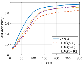
Table II shows the relationship between quantization bits and test accuracy. The proposed FLAG model exhibits a communication-learning tradeoff; that is, the higher the quantization bits, the higher the test accuracy. Additionally, when bits, the increased communication factors respectively. This means that more quantization bits can help to dilute the additional communication costs generated by encryption and reduce the increased communication factors .
| Bits | 6 | 8 | 10 |
|---|---|---|---|
| Increased Factor | 3.5 | 2.876 | 2.5 |
| Test Accuracy | 0.8487 | 0.9026 | 0.9338 |
Table III compares the performance of FLOP vs. the performance of an LWE based encryption whose error term is not eliminated (i.e., ). We adopt the same parameter setting of FLOP as before, except that the number of client is set as . The standard deviation of the error in LWE is set as . Notably, when , the overflow probability of is as large as .
| Bits | 6 | 8 | 10 |
| FLOP | 0 | 0 | 0 |
| 0.3558 | 0.0003 | 0 |
V Conclusion
In conclusion, we have introduced FLAG as a novel federated learning framework that leverages private-key encryption based on lattices. The error term in LWE is generated from a randomized quantization of the gradients. The CPA security of the scheme is proved based on the hardness of LWE over uniform errors, thus our system leaks no information of participants to the honest-but-curious parameter server. FLAG features a small probability of overflow, and achieves accuracy to close to unquantized DSGD. The experiments shed light on the adaptability of FLAG under different security parameters and highlight its potential for privacy-preserving federated learning.
References
- [1] J. Dean, G. Corrado, R. Monga, K. Chen, M. Devin, M. Mao, M. Ranzato, A. Senior, P. Tucker, K. Yang et al., “Large scale distributed deep networks,” in Advances in Neural Information Processing Systems, 2012, pp. 1223–1231.
- [2] R. Bekkerman, M. Bilenko, and J. Langford, Scaling up machine learning: Parallel and distributed approaches. Cambridge University Press, 2011.
- [3] H. B. McMahan, E. Moore, D. Ramage, and B. A. y Arcas, “Federated learning of deep networks using model averaging,” arXiv preprint arXiv:1602.05629, vol. 2, p. 2, 2016.
- [4] L. T. Phong, Y. Aono, T. Hayashi, L. Wang, and S. Moriai, “Privacy-preserving deep learning via additively homomorphic encryption,” IEEE Trans. Inf. Forensics Secur., vol. 13, no. 5, pp. 1333–1345, 2018.
- [5] L. Liu, Y. Wang, G. Liu, K. Peng, and C. Wang, “Membership inference attacks against machine learning models via prediction sensitivity,” IEEE Trans. Dependable Secur. Comput., vol. 20, no. 3, pp. 2341–2347, 2023.
- [6] M. Abadi, A. Chu, I. Goodfellow, H. B. McMahan, I. Mironov, K. Talwar, and L. Zhang, “Deep learning with differential privacy,” in Proceedings of the 2016 ACM SIGSAC conference on computer and communications security, 2016, pp. 308–318.
- [7] Ú. Erlingsson, V. Pihur, and A. Korolova, “Rappor: Randomized aggregatable privacy-preserving ordinal response,” in Proceedings of the 2014 ACM SIGSAC conference on computer and communications security, 2014, pp. 1054–1067.
- [8] R. Shokri and V. Shmatikov, “Privacy-preserving deep learning,” in Proceedings of the 22nd ACM SIGSAC conference on computer and communications security, 2015, pp. 1310–1321.
- [9] T. Stevens, C. Skalka, C. Vincent, J. Ring, S. Clark, and J. Near, “Efficient differentially private secure aggregation for federated learning via hardness of learning with errors,” in 31st USENIX Security Symposium (USENIX Security 22), 2022, pp. 1379–1395.
- [10] C. Zhang, S. Li, J. Xia, W. Wang, F. Yan, and Y. Liu, “BatchCrypt: Efficient homomorphic encryption for Cross-Silo federated learning,” in 2020 USENIX annual technical conference (USENIX ATC 20), 2020, pp. 493–506.
- [11] X. Zhang, A. Fu, H. Wang, C. Zhou, and Z. Chen, “A privacy-preserving and verifiable federated learning scheme,” in 2020 IEEE International Conference on Communications, ICC 2020, Dublin, Ireland, June 7-11, 2020. IEEE, 2020, pp. 1–6.
- [12] P. Paillier, “Public-key cryptosystems based on composite degree residuosity classes,” in International conference on the theory and applications of cryptographic techniques. Springer, 1999, pp. 223–238.
- [13] P. W. Shor, “Polynomial-time algorithms for prime factorization and discrete logarithms on a quantum computer,” SIAM review, vol. 41, no. 2, pp. 303–332, 1999.
- [14] C. Peikert, “Lattice cryptography for the internet,” in International workshop on post-quantum cryptography. Springer, 2014, pp. 197–219.
- [15] J. Wang, L. Liu, S. Lyu, Z. Wang, M. Zheng, F. Lin, Z. Chen, L. Yin, X. Wu, and C. Ling, “Quantum-safe cryptography: crossroads of coding theory and cryptography,” Science China Information Sciences, vol. 65, no. 1, p. 111301, 2022.
- [16] C. Saliba, L. Luzzi, and C. Ling, “A reconciliation approach to key generation based on module-lwe,” in 2021 IEEE International Symposium on Information Theory (ISIT). IEEE, 2021, pp. 1636–1641.
- [17] O. Regev, “On lattices, learning with errors, random linear codes, and cryptography,” Journal of the ACM (JACM), vol. 56, no. 6, pp. 1–40, 2009.
- [18] C. Gentry, “Fully homomorphic encryption using ideal lattices,” in Proceedings of the forty-first annual ACM symposium on Theory of computing, 2009, pp. 169–178.
- [19] Z. Zheng, K. Tian, and F. Liu, “Fully homomorphic encryption,” in Modern Cryptography Volume 2: A Classical Introduction to Informational and Mathematical Principle. Springer, 2022, pp. 143–174.
- [20] G. Yan, T. Li, S.-L. Huang, T. Lan, and L. Song, “Ac-sgd: Adaptively compressed sgd for communication-efficient distributed learning,” IEEE Journal on Selected Areas in Communications, vol. 40, no. 9, pp. 2678–2693, 2022.
- [21] L. Bottou, F. E. Curtis, and J. Nocedal, “Optimization methods for large-scale machine learning,” Siam Review, vol. 60, no. 2, pp. 223–311, 2018.
- [22] D. Data and S. Diggavi, “Byzantine-resilient high-dimensional federated learning,” IEEE Transactions on Information Theory, 2023.
- [23] D. Micciancio and C. Peikert, “Hardness of sis and lwe with small parameters,” in Annual cryptology conference. Springer, 2013, pp. 21–39.
- [24] J. Alwen, S. Krenn, K. Pietrzak, and D. Wichs, “Learning with rounding, revisited: New reduction, properties and applications,” in Annual Cryptology Conference. Springer, 2013, pp. 57–74.
- [25] A. Shamir, “How to share a secret,” Communications of the ACM, vol. 22, no. 11, pp. 612–613, 1979.
- [26] R. M. Gray and T. G. Stockham, “Dithered quantizers,” IEEE Transactions on Information Theory, vol. 39, no. 3, pp. 805–812, 1993.
- [27] A. Abdi and F. Fekri, “Nested dithered quantization for communication reduction in distributed training,” arXiv preprint arXiv:1904.01197, 2019.
- [28] J. Katz and Y. Lindell, Introduction to modern cryptography: principles and protocols. Chapman and hall/CRC, 2007.
- [29] N. Döttling and J. Müller-Quade, “Lossy codes and a new variant of the learning-with-errors problem,” in Advances in Cryptology–EUROCRYPT 2013: 32nd Annual International Conference on the Theory and Applications of Cryptographic Techniques, Athens, Greece, May 26-30, 2013. Proceedings 32. Springer, 2013, pp. 18–34.
- [30] D. Micciancio and M. Schultz, “Error correction and ciphertext quantization in lattice cryptography,” in Advances in Cryptology - CRYPTO 2023, ser. Lecture Notes in Computer Science, H. Handschuh and A. Lysyanskaya, Eds., vol. 14085. Springer, 2023, pp. 648–681.
- [31] Y. LeCun et al., “Lenet-5, convolutional neural networks,” URL: http://yann. lecun. com/exdb/lenet, vol. 20, no. 5, p. 14, 2015.