Non-linear Mendelian randomization with Two-stage prediction estimation and Control function estimation

Abstract

Most of the existing Mendelian randomization (MR) methods are limited by the assumption of linear causality between exposure and outcome, and the development of new non-linear MR methods is highly desirable. We introduce two-stage prediction estimation and control function estimation from econometrics to MR and extend them to non-linear causality. We give conditions for parameter identification and theoretically prove the consistency and asymptotic normality of the estimates. We compare the two methods theoretically under both linear and non-linear causality. We also extend the control function estimation to a more flexible semi-parametric framework without detailed parametric specifications of causality. Extensive simulations numerically corroborate our theoretical results. Application to UK Biobank data reveals non-linear causal relationships between sleep duration and systolic/diastolic blood pressure.

1 Introduction

The presence of unmeasured confounders in epidemiological studies usually presents a major bias for the estimation of causal effects between exposure and outcome. Mendelian randomization (MR) uses genetic variation as an instrumental variable (IV) to estimate the causal effect of exposure on outcome through the association of genetic variation with exposure and outcome, respectively Sekula et al. (2016). It is effective in avoiding confounding bias and is now widely used in epidemiological studies. The most commonly used MR methods are the ratio method as well as the two-stage least squares method, both of which rely on the linear assumption of causal effects, i.e. that each unit change in exposure produces the same effect on the outcome Burgess et al. (2017). In practice, however, this assumption may not be satisfied in many cases. For example, cohort study and meta-analysis have found obvious U-shaped correlations between sleep duration and several cardiovascular events Yin et al. (2017); Daghlas et al. (2019). Therefore, non-linear MR methods are essential.

Researchers have already noted this problem. For example, Burgess Burgess et al. (2014); Staley and Burgess (2017); Coscia et al. (2022); Mason and Burgess (2022); Tian et al. (2023), as well as Silverwood Silverwood et al. (2014), have suggested that it is possible to stratify the individuals in a certain way, treat the causal effects as linear within each stratum, use the ratio method to calculate local average causal effect within each stratum, and then portray the non-linear causal effect of exposure on the outcome by testing for heterogeneity among the stratum estimates, conducting trend tests, and fitting fractional polynomial model or piecewise linear model. Using these methods, epidemiological researchers have found many non-linear causal effects of exposure on outcomes Sun et al. (2019); Rogne et al. (2020); Ai et al. (2021). Sulc et al. Sulc et al. (2022) instead used polynomials to model the non-linear causal relationship between exposure and outcome, again using a two-stage approach to estimate the coefficients of each polynomial term. While these methods have been widely used in applications, the theoretical properties of the estimators have not been verified.

The presence of unmeasured confounders is likewise an important issue and is referred to as endogeneity in economic studies. Economists have also developed a number of methods to deal with unmeasured confounders. The most commonly used of these are two-stage prediction estimation and control function estimation Horowitz (2011); Terza et al. (2008). Both methods exhibit good performance under linear causality but differs when extended to non-linear causality Guo and Small (2016); Terza et al. (2008).

In this article, we introduce two-stage prediction estimation and control function estimation from economics to MR and further refine and extend them. We give conditions for parameter identification under non-linear causality for both methods, theoretically prove the consistency and asymptotic normality of the estimators, compare the two estimates under linear and non-linear causality, and extend the control function estimation to a more flexible semi-parametric framework. We validated our results numerically using a large number of simulation experiments and applied the methods to UK Biobank (UKB) data to investigate the causal relationship between sleep duration and systolic/diastolic blood pressure.

The paper is organized as follows: in Section 2 we give the parameter identification conditions for the two methods, in Section 3 we prove the consistency and asymptotic normality of the estimates and compare the two methods in both linear and non-linear causality, in Section 4 we give a more flexible framework for semi-parametric estimation, in Section 5 we perform numerical simulation experiments, in Section 6 we apply the methods to UKB data, and Section 7 and Section 8 contain our discussion and conclusions, respectively. All proofs are placed in the Appendix.

2 Identification

2.1 Setup and notation

We have i.i.d. observations $\{(Z_{i},C_{i},X_{i},Y_{i})\}_{i=1}^{n}$ from a super-population $(Z,C,X,Y)$ where $Z$ is the IV, $C$ is the measured covariate, $X$ is the exposure variable, $Y$ is the outcome, $U$ is the unmeasured confounder. For IV estimation, $Z$ should meet three core assumptions: (1) $Z$ has an effect on the exposure $X$; (2) $Z$ is independent of the unmeasured confounder $U$; (3) $Z$ is independent of outcome $Y$ given $X,C$ and $U$. In addition, we also assume $Z\Vbar C$ and $C\Vbar U$. The relationship could be depicted using Figure 1.

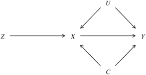
Figure 1: The Causal Graph for $(Z,C,U,X,Y)$ with $U$ the unmeasured confounder.

Considering the the most prevalent additive genetic model, it is natural to assume that the effect of $Z$ on $X$ is linear. Without loss of generality, we also assume that the causal effects of $C,U$ on $X$ is linear, but the causal effects on $Y$ can be non-linear. Distinguishing from linear MR, we consider the case where $X$ has a non-linear causal effect on $Y$, denoting as $f(X)$. Thus, we have the following equations:

$$X=\beta_{X0}+\beta_{Z}Z+\beta_{C}C+\beta_{U}U+\epsilon_{X}$$ (1)

$$Y=\beta_{Y0}+f(X)+g(C)+h(U)+\epsilon_{Y}$$ (2)

where $\epsilon_{X}$ and $\epsilon_{Y}$ are the random error terms with $E(\epsilon_{X})=0,E(\epsilon_{Y})=0$. $f(X)$ and $g(C)$ can be composed of several different basis functions, i.e., $f(X)=\sum_{j=1}^{K_{1}}\theta_{j}f_{j}(X)$, $g(C)=\sum_{j=1}^{K_{2}}\gamma_{j}g_{j}(C)$. Matrix $F=[1,f_{1}(X),\ldots,f_{K_{1}}(X)]$ and matrix $G=[1,g_{1}(C),\ldots,g_{K_{2}}(C)]$ are both full column rank. There can also be multiple IVs, but it is required that these IVs are linearly independent, and the measeured covariates are the same.

Then we can estimate $\beta_{Y0},\theta_{1},\ldots,\theta_{K_{1}},\gamma_{1},\ldots,\gamma_{K_{2}}$ using the following two methods.

2.2 Two-stage prediction estimation

Rewrite equation 2 as:

$$\begin{split}Y&=\beta_{Y0}+\sum_{j=1}^{K_{1}}\theta_{j}\hat{f}_{j}(X)+\sum_{j=1}^{K_{2}}\gamma_{j}g_{j}(C)+\\ &\quad\sum_{j=1}^{K_{1}}\theta_{j}\left(f_{j}(X)-\hat{f}_{j}(X)\right)+h(U)+\epsilon_{Y}\end{split}$$ (3)

where $\hat{f}_{j}(X)$ is the fitted values of linear regression $f_{j}(X)\sim Z+C,j=1,2,\ldots,K_{1}$. It can be proved that

$$E(Y|\hat{f}(X),g(C))=\beta_{Y0}+\sum_{j=1}^{K_{1}}\theta_{j}\hat{f}_{j}(X)+\sum_{j=1}^{K_{2}}\gamma_{j}g_{j}(C)$$

So we can fit the regression of $Y\sim\hat{f}_{1}(X)+\hat{f}_{2}(X)+\ldots+\hat{f}_{K_{1}}(X)+g_{1}(C)+g_{2}(C)+\ldots+g_{K_{2}}(C)$ to get the estimates of $\beta_{Y0},\theta_{1},\ldots,\theta_{K_{1}},\gamma_{1},\ldots,\gamma_{K_{2}}$.

Theorem 1.

Denote the number of IVs and the number of measured covariates as $n_{1}$ and $n_{2}$, respectively. The number of linear functions of $C$ in $g_{1}(C),g_{2}(C),\ldots,g_{k2}(C)$ is $k$. Then, the parameters $\beta_{Y0},\theta_{1},\ldots,\theta_{K_{1}},\gamma_{1},\ldots,\gamma_{K_{2}}$ can be identified if and only if $K_{1}+k\leq(n_{1}+n_{2})$.

The proof of Theorem 1 is placed in Appendix A.

Remark 1.

When $f(X)=X$ as well as $g(C)=C$, the two-stage prediction estimation degenerates into the ordinary two-stage least squares estimation. Different from the parameter identification condition $(K_{1}\leq n_{1})$ of the ordinary two-stage least squares estimation, we allow for the non-linear causality of both $X$ and $C$ on $Y$ and take the form of causality (linear or non-linear) between $C$ and $Y$ into account in the parameter identification condition.

2.3 Control function estimation

Rewrite equation 1 and 2 as:

$$X=\beta_{X0}+\beta_{Z}Z+\beta_{C}C+\delta_{1}$$ (4)

$$Y=\beta_{Y0}+f(X)+g(C)+\delta_{2}$$ (5)

where $\delta_{1}=\beta_{U}U+\epsilon_{X},\delta_{2}=h(U)+\epsilon_{Y}$. Assume that the relationship between $\delta_{2}$ and $\delta_{1}$ is linear, i.e. $\delta_{2}=\rho\delta_{1}+e,\delta_{1}\Vbar e$. Then we have

$$Y=\beta_{Y0}+f(X)+g(C)+\rho\hat{\delta}_{1}+\rho(\delta_{1}-\hat{\delta}_{1})+e$$ (6)

where $\hat{\delta}_{1}$ is the residuals of the linear regression $X\sim Z+C$. It can be proved that

$$E(Y|f(X),g(C),\hat{\delta}_{1})=\beta_{Y0}+f(X)+g(C)+\rho\hat{\delta}_{1}$$

So we can fit the regression of $Y\sim f_{1}(X)+\ldots+f_{K_{1}}(X)+g_{1}(C)+\ldots+g_{K_{2}}(C)+\hat{\delta}_{1}$ to get the estimates of $\beta_{Y0},\theta_{1},\ldots,\theta_{K_{1}},\gamma_{1},\ldots,\gamma_{K_{2}}$.

Theorem 2.

The parameters $\beta_{Y0},\theta_{1},\ldots,\theta_{K_{1}},\gamma_{1},\ldots,\gamma_{K_{2}}$ can be identified when $\delta_{2}=\rho\delta_{1}+e(\delta_{1}\Vbar e)$.

The proof of Theorem 2 is placed in Appendix B.

Remark 2.

The parameter identification condition of the control function estimation has been stated by several researchers in economics Guo and Small (2016); Wooldridge (2015). We state that, different from two-stage prediction estimation, the control function estimation has no requirements on the number of IVs, measures covariates and the form of causality (linear or non-linear) between $C$ and $Y$.

3 Estimation

3.1 Two-stage prediction estimation

In the first stage, we fit the regression of $f_{j}(X)\sim Z+C$ and get the fitted values $\hat{f}_{j}(X),j=1,2,\ldots,K_{1}$. Then in the second stage, we fit the regression of $Y\sim\hat{f}_{1}(X)+\hat{f}_{2}(X)+\ldots+\hat{f}_{K_{1}}(X)+g_{1}(C)+g_{2}(C)+\ldots+g_{K_{2}}(C)$ to get the estimates of $\beta_{Y0},\theta_{1},\theta_{2},\ldots,\theta_{K_{1}},\gamma_{1},\gamma_{2},\ldots,\gamma_{K_{2}}$, denoting as $\hat{B}_{2SP}$. And the true value of parameters $\beta_{Y0},\theta_{1},\theta_{2},\ldots,\theta_{K_{1}},\gamma_{1},\gamma_{2},\ldots,\gamma_{K_{2}}$ is denoted as $B$.

Theorem 3.

Under the assumption that: $K_{1}+k\leq(n_{1}+n_{2})$ and $g(C)$ is a linear function of C, we have

$$\hat{B}_{2SP}\stackrel{{\scriptstyle p}}{{\rightarrow}}B$$

$$\sqrt{n}(\hat{B}_{2SP}-B)\stackrel{{\scriptstyle d}}{{\rightarrow}}N(0,\Sigma_{2SP})$$

where $\Sigma_{2SP}$ is the asymptotic variance of $\sqrt{n}(\hat{B}_{2SP}-B)$ and is equal to $E(V^{\prime}V)^{-1}Var(\delta_{2}),V=[1,\hat{f}_{1},\hat{f}_{2},\ldots,\hat{f}_{K_{1}},g_{1},g_{2},\ldots,g_{K_{2}}]$.

The assumption of $K_{1}+k\leq(n_{1}+n_{2})$ is to ensure that the parameters are identifiable. The proof of Theorem 3 is placed in Appendix C.

Remark 3.

Distinguishing ourselves from other studies on two-stage prediction estimation, we consider the effect of the form of causality of $C$ on $Y$ on obtaining a consistent estimate and give the exact formula for the asymptotic variance in the case where the causality between $X$ and $Y$ is non-linear. According to Theorem 3, we can obtain a consistent estimate of $B$ and the corresponding asymptotic variance using observed data, so that we can perform the hypothesis test $H_{0}:B=0$ to test whether the non-linear causality is statistically significant directly.

3.2 Control function estimation

In the first stage, we fit the regression of $X\sim Z+C$ and get the residuals $\hat{\delta}_{1}$. Then in the second stage, we fit the regression of $Y\sim f_{1}(X)+f_{2}(X)+\ldots+f_{K_{1}}(X)+g_{1}(C)+g_{2}(C)+\ldots+g_{K_{2}}(C)+\hat{\delta}_{1}$ to get the estimates of $\beta_{Y0},\theta_{1},\theta_{2},\ldots,\theta_{K_{1}},\gamma_{1},\gamma_{2},\ldots,\gamma_{K_{2}}$, denoting as $\hat{B}_{CF}$.

Theorem 4.

Under the assumption that $\delta_{2}=\rho\delta_{1}+e(\delta_{1}\Vbar e)$, we have

$$\hat{B}_{CF}\stackrel{{\scriptstyle p}}{{\rightarrow}}B$$

$$\sqrt{n}(\hat{B}_{CF}-B)\stackrel{{\scriptstyle d}}{{\rightarrow}}N(0,\Sigma_{CF})$$

where $\Sigma_{CF}$ is the asymptotic variance of $\sqrt{n}(\hat{B}_{CF}-B)$. (The exact form of $\Sigma_{CF}$ is somewhat complicated, and we place it in Appendix D.2.)

The proof of Theorem 4 is placed in Appendix D.

Remark 4.

Similar to Theorem 3, according to Theorem 4, we can obtain a consistent estimate of $B$ and the corresponding asymptotic variance using observed data by control function estimation, so that we can perform the hypothesis test $H_{0}:B=0$ to test whether the non-linear causality is statistically significant directly.

3.3 Comparison of the two methods

Theorem 5.

On the basis that the assumptions of Theorems 1-4 are satisfied, the control function estimation is equivalent to the two-stage prediction estimation when the causality between $X$ and $Y$ is linear, and the control function estimation is more efficient than the two-stage prediction estimation when the causality between $X$ and $Y$ is non-linear.

We give the proof of Theorem 5 in the Appendix E.

Remark 5.

Different from Guo and Small’s Guo and Small (2016) study, we compare two-stage prediction estimation and control function estimation from two aspects: first, the conditions for parameter identification and consistency of estimators (Theorem 1,2,3,4); and second, the asymptotic variance of the estimates of the two methods when the assumptions required for both methods are satisfied (Theorem 5).

4 Flexible semi-parametric MR

Considering the good performance of control function estimation when non-linear causality is present, we can further extend it to more flexible semi-parametric case. In concrete terms, we fit the linear regression of $X\sim Z+C$ and get the residuals $\hat{\delta}_{1}$ just as before. But in the second stage we adopt a non-parametric estimation, using a flexible specification for $f(X)$, instead of the original detailed parametric estimation.

By Theorem 4 we know that fitting the regression of $Y\sim f_{1}(X)+f_{2}(X)+\ldots+f_{K_{1}}(X)+g(C)+\hat{\delta}_{1}$ in the second stage yields consistent and asymptotically normal estimates of $\theta_{j},j=1,2,\ldots,K_{1}$. Thus we can represent $f(X)$ using spline bases and fit non-parametric penalized spline regression of $Y\sim s(X)+s(C)+\hat{\delta}_{1}$ to estimate $f(X)$ in the second stage. Given the property of spline smoothers Perperoglou et al. (2019), it is possible to obtain an estimate of $f(X)$ with a very small approximation error as well as a very small tendency to overfitting.

5 Simulation

We performed simulations in both the parametric and semi-parametric cases. In the parametric case we specified the form of $f(X)$ in advance and estimated its coefficient, while in the semi-parametric case we fitted the form of $f(X)$ using splines. Comparisons were made between the performance of two-stage prediction estimation and control function estimation under different sample sizes ($N=5000,10000,20000,50000$) and different IV strengths (proportion of exposure variance explained by IV (PVE) $=25\%,50\%,75\%$).

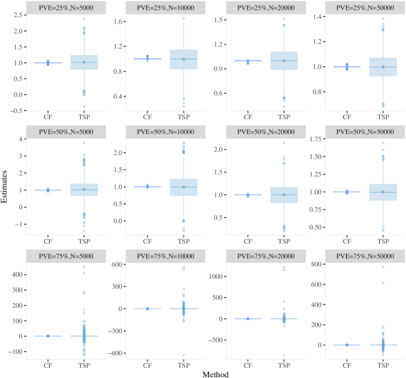
Figure 2: Simulation results for the parametric case. We run $1000$ simulations in each setting. The diamond represents the position of the mean value. PVE: proportion of exposure variance explained by instrumental variable; N: sample size; CF: control function estimation; TSP: two-stage prediction estimation.

In both cases, $Z,C,U,\epsilon_{X},e$ were sampled from standard normal distribution independently, $X$ and $Y$ were generated according to the following equations, with PVE changed by varying the value of $\beta_{Z}$.

$$\delta_{1}=U+\epsilon_{X}$$

$$\delta_{2}=\delta_{1}+e$$

$$X=1+\beta_{Z}Z+C+\delta_{1}$$

$$Y=1+f(X)+C+\delta_{2}$$

Parametric Case: We set $f(X)=sin(X)$ and estimated its coefficients using both two-stage prediction estimation and control function estimation. Figure 2 illustrates the performance of the two methods for different IV strengths and different sample sizes (here the true true coefficient of $f(X)$ is $1$). It can be seen that the control function method yields accurate and robust estimates in all cases. But the two-stage prediction method shows a larger variance, especially when the IV is stronger $(PVE=75\%)$ (Figure 2).

Semi-parametric Case: In this case, it is assumed that we do not have information about the exact form of $f(X)$ ahead of time, the two-stage prediction method cannot be used, and we only estimate using the control function method. We considered four different $f(X):X,(X/3)^{2},sin(X)$, and $e^{X/3}$. In the first stage a linear regression of $X\sim Z+C$ was fitted to obtain the residuals $\hat{\delta}_{1}$ as in the parametric case, but in the second stage a penalized spline regression of $Y\sim s(X)+C+\hat{\delta}_{1}$ was fitted, where $s(X)$ denotes the smooth function of $X$, the exact form of which needs to be estimated from the data. We used cubic splines for stage two. Figure 3 illustrates the estimates of $f(X)$ by this semi-parametric control function method at a sample size of $5000$ and $PVE=25\%$. It is easy to see that even with smaller sample size and weaker IV strength the method shows good performance in estimating the specific form of $f(X)$, especially in the denser range of the data (Figure 3).

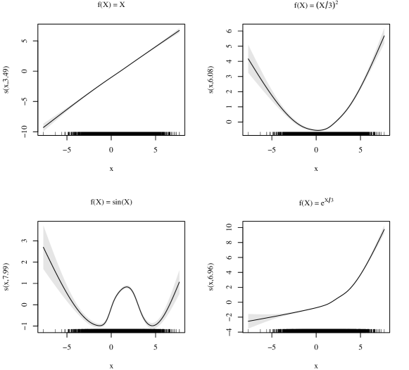
Figure 3: Simulation results for the semi-parametric case. The title of each subgraph is $f(X)$ set at the time of data generation.

6 Real data

We applied our methods to UKB real data to investigate the potential causal effect of sleep duration on systolic as well as diastolic blood pressure. UKB is a large biomedical database containing over 500000 UK participants Bycroft et al. (2018). From this database, we selected White British participants, excluding individuals identified as outliers in heterozygosity and missing rates, excluding individuals with inconsistent genetic and self-reported sex, excluding individuals with ten or more third-degree relatives identified and individuals excluded from the kinship inference process, and excluding individuals missing the exposure, outcome, and covariates we wanted to study.

We obtained 78 genetic variations significantly associated with sleep duration from a large-scale genome-wide association study of sleep duration in a population of European descent Dashti et al. (2019) and used unweighted polygenic risk scores for these 78 genetic variations as IV. Mode interpolation was used for missing genotypes. Data on sleep duration were obtained from participants’ self-reports, and individuals with extreme data ($<3$h or $>18$h) were excluded Dashti et al. (2019). Systolic and diastolic blood pressure were averaged using two independent automated measurements. For individuals taking antihypertensive medication, we corrected systolic and diastolic blood pressure by increasing 15 and 10 mmHg, respectively Evangelou et al. (2018). In addition, we adjusted for the covariates of age, sex, measurement center, genotyping chip, and the first 10 genetic principal components in both stages of the regression. All of the above data were obtained at the initial visit. A total of 402460 participants were ultimately included in the analysis.

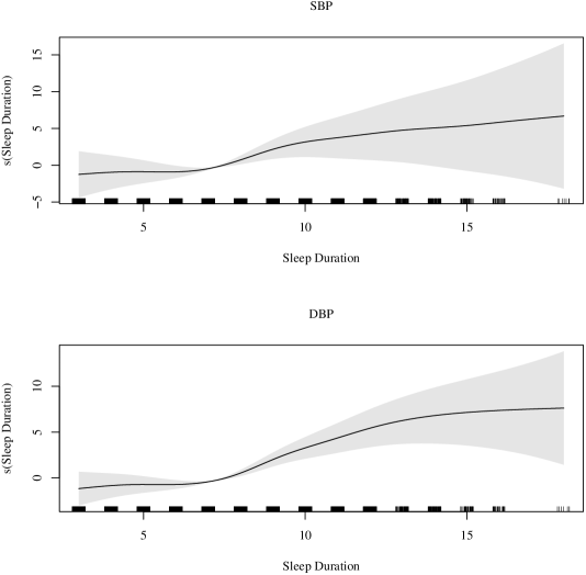
Figure 4: Results of real data application. SBP: systolic blood pressure; DBP: diastolic blood pressure.

In the first stage, we fitted linear regression of sleep duration on IV as well as covariates to obtain residuals. In the second stage, we fitted penalized spline regressions of systolic/diastolic blood pressure on sleep duration, residuals obtained from the first stage, and the covariates. Figure 4 gives the curves for the causal effect of sleep duration on systolic and diastolic blood pressure derived from the use of cubic spline in the second stage. The estimated causal effects of sleep duration on systolic and diastolic blood pressure show a similar pattern, with changes in sleep duration having a flat effect on systolic/diastolic blood pressure when sleep duration is shorter than 7 hours, and prolonged sleep duration elevating systolic/diastolic blood pressure when sleep duration is longer than 7 hours.

7 Discussion

Non-linear MR methods, although they have been used in many epidemiological studies, have always lacked a theoretical proof of the mathematical properties of the estimators. In this paper, we systematically give a theoretical study of two-stage prediction estimation and control function estimation, including the identification condition, consistency and asymptotic normality of the estimates, and the difference between two methods in both linear and non-linear causality. Overall, compared to the two-stage prediction estimation, the control function estimation is more robust in causal parameter estimating and more flexible in causal function form specification.

MR analysis has been widely used in epidemiologic studies in recent years due to its good performance in dealing with confounding bias, and has gradually developed into an important epidemiologic research method. While using MR researchers must recognize the need for caution in interpreting its results. Currently widely used MR methods such as inverse variance weighted method Burgess et al. (2016), MR-Egger regression method Bowden et al. (2015), weighted median method Bowden et al. (2016), and weighted mode method Hartwig et al. (2017) all rely on the assumption that the causal effect between exposure and outcome is linear. When this assumption is not satisfied, the estimates obtained using these methods will no longer be the conditional average treatment effect we are interested in, missing much of practical significance. However, the causal relationship between exposure and outcome in many cases cannot be described by a straight line simply. Thus the development and use of MR methods applicable to non-linear causality is essential.

In terms of non-linear MR methods, a great deal of work has been done by Burgess et al Burgess et al. (2014); Staley and Burgess (2017); Tian et al. (2023). They have developed a series of stratification-based non-linear MR methods and have used them to discover many non-linear causal relationships between exposures and outcomes. In contrast to the approach of Burgess et al, our approach does not stratify exposures, but rather tests the possible non-linear effects of exposure on outcomes using exposure data at all levels. For both two-stage prediction estimation and control function estimation, we give identification and consistency conditions as well as the asymptotic variance that allows the researchers to perform hypothesis testing on the coefficients directly. We also compare the two methods in both linear and non-linear cases, to facilitate the researcher’s choice of the appropriate method depending on the specific exposure and outcome scenarios to be analyzed. In addition, we provide a more flexible semi-parametric estimation framework, which is more recommended if the researchers do not have any a priori knowledge about the causal relationship to be investigated.

In the simulation experiments, under non-linear causality, we observe that the variance of the two-stage prediction estimates is relatively large, especially when the IV is of high strength. It is understandable that due to the linear association between exposure and IV, the relationship between the non-linear term of exposure and IV is inevitably non-linear, and thus the estimation instability occurs when we use IV to linearly predict the non-linear term of exposure. This situation is more likely to occur when the IV strength is large or when the non-linear term of exposure deviates from linearity heavily. In the real data application, sleep duration data were derived from participants’ self-reports and took all integer values. This leaves few values of sleep duration less than 7 hours (only 3,4,5,6), which may be a contributing factor to the fact that we did not observe an apparent causal effect of sleep duration on systolic/diastolic blood pressure when sleep duration was shorter than 7 hours.

It should be noted that our approach still has some limitations. For example, our method is a one-sample MR method, which still needs to use individual level data for estimation. But considering that more and more excellent large cohorts are now opening up their data requests to researchers, we do not see this as an insurmountable difficulty. In addition, the current two-stage prediction estimation and control function estimation rely on a number of assumptions, and how to obtain good estimates in relaxing these assumptions needs for further research. Finally, in this article we have only studied the case where both exposure and outcome are continuous variables, and estimation when the variables are in other forms deserves to be studied further.

8 Conclusions

Both two-stage prediction estimation and control function estimation can yield consistent and asymptotically normal estimates under specific conditions. The control function estimation is much more robust than two-stage prediction estimation under non-linear causality. In addition, the control function estimation can be extended to a more flexible semi-parametric framework without making detailed parametric assumptions about the form of the causal effect.

The Authors declare that there is no conflict of interest

This work was supported by Peking University.

References

- Ai et al. (2021) Ai S, Zhang J, Zhao G, Wang N, Li G, So HC, Liu Y, Chau SWH, Chen J, Tan X, Jia F, Tang X, Shi J, Lu L and Wing YK (2021) Causal associations of short and long sleep durations with 12 cardiovascular diseases: linear and nonlinear mendelian randomization analyses in uk biobank. EUROPEAN HEART JOURNAL 42(34): 3349+. 10.1093/eurheartj/ehab170.
- Bowden et al. (2015) Bowden J, Smith GD and Burgess S (2015) Mendelian randomization with invalid instruments: effect estimation and bias detection through egger regression. INTERNATIONAL JOURNAL OF EPIDEMIOLOGY 44(2): 512–525. 10.1093/ije/dyv080.
- Bowden et al. (2016) Bowden J, Smith GD, Haycock PC and Burgess S (2016) Consistent estimation in mendelian randomization with some invalid instruments using a weighted median estimator. GENETIC EPIDEMIOLOGY 40(4): 304–314. 10.1002/gepi.21965.
- Burgess et al. (2014) Burgess S, Davies NM, Thompson SG and Consortium EI (2014) Instrumental variable analysis with a nonlinear exposure-outcome relationship. EPIDEMIOLOGY 25(6): 877–885. 10.1097/EDE.0000000000000161.
- Burgess et al. (2016) Burgess S, Dudbridge F and Thompson SG (2016) Combining information on multiple instrumental variables in mendelian randomization: comparison of allele score and summarized data methods. STATISTICS IN MEDICINE 35(11): 1880–1906. 10.1002/sim.6835.
- Burgess et al. (2017) Burgess S, Small DS and Thompson SG (2017) A review of instrumental variable estimators for mendelian randomization. STATISTICAL METHODS IN MEDICAL RESEARCH 26(5, SI): 2333–2355. 10.1177/0962280215597579.
- Bycroft et al. (2018) Bycroft C, Freeman C, Petkova D, Band G, Elliott LT, Sharp K, Motyer A, Vukcevic D, Delaneau O, O’Connell J, Cortes A, Welsh S, Young A, Effingham M, McVean G, Leslie S, Allen N, Donnelly P and Marchini J (2018) The uk biobank resource with deep phenotyping and genomic data. NATURE 562(7726): 203+. 10.1038/s41586-018-0579-z.
- Coscia et al. (2022) Coscia C, Gill D, Benitez R, Perez T, Malats N and Burgess S (2022) Avoiding collider bias in mendelian randomization when performing stratified analyses. EUROPEAN JOURNAL OF EPIDEMIOLOGY 37(7): 671–682. 10.1007/s10654-022-00879-0.
- Daghlas et al. (2019) Daghlas I, Dashti HS, Lane J, Aragam KG, Rutter MK, Saxena R and Vetter C (2019) Sleep duration and myocardial infarction. Journal of the American College of Cardiology 74(10): 1304—1314. 10.1016/j.jacc.2019.07.022. URL https://europepmc.org/articles/PMC6785011.
- Dashti et al. (2019) Dashti HS, Jones SE, Wood AR, Lane JM, van Hees VT, Wang H, Rhodes JA, Song Y, Patel K, Anderson SG, Beaumont RN, Bechtold DA, Bowden J, Cade BE, Garaulet M, Kyle SD, Little MA, Loudon AS, Luik A I, Scheer FAJL, Spiegelhalder K, Tyrrell J, Gottlieb DJ, Tiemeier H, Ray DW, Purcell SM, Frayling TM, Redline S, Lawlor DA, Rutter MK, Weedon MN and Saxena R (2019) Genome-wide association study identifies genetic loci for self-reported habitual sleep duration supported by accelerometer-derived estimates. NATURE COMMUNICATIONS 10. 10.1038/s41467-019-08917-4.
- Evangelou et al. (2018) Evangelou E, Warren HR, Mosen-Ansorena D, Mifsu B, Pazoki R, Gao H, Ntritsos G, Dimou N, Cabrer CP, Karaman I, Ng F, Evangelou M, Witkowska K, Tzanis E, Hellwege JN, Giri A, Edwards DRV, Sun Y V, Cho K, Gaziano JM, Wilson PWF, Tsao PS, Kovesdy CP, Esko T, Magi R, Milani L, Almgren P, Boutin T, Debette S, Ding J, Giulianini F, Holliday EG, Jackson AU, Li-Gao R, Lin WY, Luan J, Mangino M, Oldmeadow C, Prins BP, Qian Y, Sargurupremraj M, Shah N, Surendran P, Theriault S, Verweij N, Willems SM, Zhao JH, Amouyel P, Connell J, de Mutsert R, Doney ASF, Farrall M, Menni C, Morris AD, Noordam R, Pare G, Poulter NR, Shields DC, Stanton A, Thom S, Abecasis G, Amin N, Arking DE, Ayers KL, Barbieri CM, Batini C, Bis JC, Blake T, Bochud M, Boehnke M, Boerwinkle E, Boomsma D I, Bottinger EP, Braund PS, Brumat M, Campbell A, Campbell H, Chakravarti A, Chambers JC, Chauhan G, Ciullo M, Cocca M, Collins F, Cordell HJ, Davies G, de Borst MH, de Geus EJ, Deary IJ, Deelen J, Del Greco FM, Demirkale CY, Doerr M, Ehret GB, Elosua R, Enroth S, Erzurumluoglu AM, Ferreira T, Franberg M, Franco OH, Gandin I, Gasparini P, Giedraitis V, Gieger C, Girotto G, Goel A, Gow AJ, Gudnason V, Guo X, Gyllensten U, Hamsten A, Harris TB, Harris SE, Hartman CA, Havulinna AS, Hicks AA, Hofer E, Hofman A, Hottenga JJ, Huffman JE, Hwang SJ, Ingelsson E, James A, Jansen R, Jarvelin MR, Joehanes R, Johansson A, Johnson AD, Joshi PK, Jousilahti P, Jukema JW, Jula A, Kahonen M, Kathiresan S, Keavney BD, Khaw KT, Knekt P, Knight J, Kolcic I, Kooner JS, Koskinen S, Kristiansson K, Kutalik Z, Laan M, Larson M, Launer LJ, Lehne B, Lehtimaki T, Liewald DCM, Lin L, Lind L, Lindgren CM, Liu Y, Loos RJF, Lopez LM, Lu Y, Lyytikainen LP, Mahajan A, Mamasoula C, Marrugat J, Marten J, Milaneschi Y, Morgan A, Morris AP, Morrison AC, Munson PJ, Nalls MA, Nandakumar P, Nelson CP, Niiranen T, Nolte IM, Nutile T, Oldehinkel AJ, Oostra BA, O’Reilly PF, Org E, Padmanabhan S, Palmas W, Palotie A, Pattie A, Penninx BWJH, Perola M, Peters A, Polasek O, Pramstaller PP, Nguyen QT, Raitakari OT, Ren M, Rettig R, Rice K, Ridker PM, Ried JS, Riese H, Ripatti S, Robino A, Rose LM, Rotter J I, Rudan I, Ruggiero D, Saba Y, Sala CF, Salomaa V, Samani NJ, Sarin AP, Schmidt R, Schmidt H, Shrine N, Siscovick D, Smith A V, Snieder H, Sober S, Sorice R, Starr JM, Stott DJ, Strachan DP, Strawbridge RJ, Sundstrom J, Swertz MA, Taylor KD, Teumer A, Tobin MD, Tomaszewski M, Toniolo D, Traglia M, Trompet S, Tuomilehto J, Tzourio C, Uitterlinden AG, Vaez A, van der Most PJ, van Duijn CM, Vergnaud AC, Verwoert GC, Vitart V, Voelker U, Vollenweider P, Vuckovic D, Watkins H, Wild SH, Willemsen G, Wilson JF, Wright AF, Yao J, Zemunik T, Zhang W, Attia JR, Butterworth AS, Chasman D, Conen D, Cucca F, Danesh J, Hayward C, Howson JMM, Laakso M, Lakatta EG, Langenberg C, Melander O, Mook-Kanamori DO, Palmer CNA, Risch L, Scott RA, Scott RJ, Sever P, Spector TD, van der Harst P, Wareham NJ, Zeggini E, Levy D, Munroe PB, Newton-Cheh C, Brown MJ, Metspalu A, Hung AM, O’Donnell C, Edwards TL, Psaty BM, Tzoulaki I, Barnes MR, Wain L V, Elliott P, Caulfield MJ and Program MV (2018) Genetic analysis of over 1 million people identifies 535 new loci associated with blood pressure traits. NATURE GENETICS 50(10): 1412+. 10.1038/s41588-018-0205-x.
- Guo and Small (2016) Guo Z and Small DS (2016) Control function instrumental variable estimation of nonlinear causal effect models. JOURNAL OF MACHINE LEARNING RESEARCH 17.
- Hartwig et al. (2017) Hartwig FP, Smith GD and Bowden J (2017) Robust inference in summary data mendelian randomization via the zero modal pleiotropy assumption. INTERNATIONAL JOURNAL OF EPIDEMIOLOGY 46(6): 1985–1998. 10.1093/ije/dyx102.
- Horowitz (2011) Horowitz JL (2011) Applied nonparametric instrumental variables estimation. ECONOMETRICA 79(2): 347–394. 10.3982/ECTA8662.
- Mason and Burgess (2022) Mason AM and Burgess S (2022) Software application profile: Sumnlmr, an r package that facilitates flexible and reproducible non-linear mendelian randomization analyses. INTERNATIONAL JOURNAL OF EPIDEMIOLOGY 51(6): 2014–2019. 10.1093/ije/dyac150.
- Perperoglou et al. (2019) Perperoglou A, Sauerbrei W, Abrahamowicz M, Schmid M and Initiative TS (2019) A review of spline function procedures in r. BMC MEDICAL RESEARCH METHODOLOGY 19. 10.1186/s12874-019-0666-3.
- Rogne et al. (2020) Rogne T, Solligard E, Burgess S, Brumpton BM, Paulsen J, Prescott HC, Mohus RM, Gustad LT, Mehl A, Asvold BO, DeWan AT and Damas JK (2020) Body mass index and risk of dying from a bloodstream infection: A mendelian randomization study. PLOS MEDICINE 17(11). 10.1371/journal.pmed.1003413.
- Sekula et al. (2016) Sekula P, Del Greco FM, Pattaro C and Koettgen A (2016) Mendelian randomization as an approach to assess causality using observational data. JOURNAL OF THE AMERICAN SOCIETY OF NEPHROLOGY 27(11): 3253–3265. 10.1681/ASN.2016010098.
- Silverwood et al. (2014) Silverwood RJ, Holmes MV, Dale CE, Lawlor DA, CWhittaker J, Smith GD, Leon DA, Palmer T, Keating BJ, Zuccolo L, Casas JP, Dudbridge F and Consortium AA (2014) Testing for non-linear causal effects using a binary genotype in a mendelian randomization study: application to alcohol and cardiovascular traits. INTERNATIONAL JOURNAL OF EPIDEMIOLOGY 43(6): 1781–1790. 10.1093/ije/dyu187.
- Staley and Burgess (2017) Staley JR and Burgess S (2017) Semiparametric methods for estimation of a nonlinear exposure-outcome relationship using instrumental variables with application to mendelian randomization. GENETIC EPIDEMIOLOGY 41(4): 341–352. 10.1002/gepi.22041.
- Sulc et al. (2022) Sulc J, Sjaarda J and Kutalik Z (2022) Polynomial mendelian randomization reveals non-linear causal effects for obesity-related traits. HUMAN GENETICS AND GENOMICS ADVANCES 3(3). 10.1016/j.xhgg.2022.100124.
- Sun et al. (2019) Sun YQ, Burgess S, Staley JR, Wood AM, Bell S, Kaptoge SK, Guo Q, Bolton TR, Mason AM, Butterworth AS, Di Angelantonio E, Vie GA, Bjorngaard JH, Kinge JM, Chen Y and Mai XM (2019) Body mass index and all cause mortality in hunt and uk biobank studies: linear and non-linear mendelian randomisation analyses. BMJ-BRITISH MEDICAL JOURNAL 364. 10.1136/bmj.l1042.
- Terza et al. (2008) Terza JV, Basu A and Rathouz PJ (2008) Two-stage residual inclusion estimation: Addressing endogeneity in health econometric modeling. JOURNAL OF HEALTH ECONOMICS 27(3): 531–543. 10.1016/j.jhealeco.2007.09.009.
- Tian et al. (2023) Tian H, Mason AM, Liu C and Burgess S (2023) Relaxing parametric assumptions for non-linear mendelian randomization using a doubly-ranked stratification method. PLOS GENETICS 19(6). 10.1371/journal.pgen.1010823.
- Wooldridge (2015) Wooldridge JM (2015) Control function methods in applied econometrics. JOURNAL OF HUMAN RESOURCES 50(2): 420–445. 10.3368/jhr.50.2.420.
- Yin et al. (2017) Yin J, Jin X, Shan Z, Li S, Huang H, Li P, Peng X, Peng Z, Yu K, Bao W, Yang W, Chen X and Liu L (2017) Relationship of sleep duration with all-cause mortality and cardiovascular events: A systematic review and dose-response meta-analysis of prospective cohort studies. JOURNAL OF THE AMERICAN HEART ASSOCIATION 6(9). 10.1161/JAHA.117.005947.