Simulation of Graph Algorithms with Looped Transformers

Abstract

The execution of graph algorithms using neural networks has recently attracted significant interest due to promising empirical progress. This motivates further understanding of how neural networks can replicate reasoning steps with relational data. In this work, we study the ability of transformer networks to simulate algorithms on graphs from a theoretical perspective. The architecture that we utilize is a looped transformer with extra attention heads that interact with the graph. We prove by construction that this architecture can simulate algorithms such as Dijkstra’s shortest path algorithm, Breadth- and Depth-First Search, and Kosaraju’s strongly connected components algorithm. The width of the network does not increase with the size of the input graph, which implies that the network can simulate the above algorithms for any graph. Despite this property, we show that there is a limit to simulation in our solution due to finite precision. Finally, we show a Turing Completeness result with constant width when the extra attention heads are utilized.

1 Introduction

Recent advancements in neural network models have significantly impacted various domains, most notably vision Yuan et al. (2021); Khan et al. (2022); Dehghani et al. (2023), and natural language processing Wei et al. (2022b); Touvron et al. (2023). Transformers Vaswani et al. (2017), at the forefront of these developments, have become standard for a wide range of complex tasks. These successes have also shed light on the capabilities of neural networks in algorithmic reasoning Veličković and Blundell (2021), such as basic arithmetic Lee et al. (2024), sorting Tay et al. (2020); Yan et al. (2020); Rodionov and Prokhorenkova (2023), dynamic programming Dudzik and Veličković (2022); Ibarz et al. (2022) and execution of graph algorithms Veličković et al. (2022); Cappart et al. (2023).

In this work, we focus on algorithmic reasoning on graphs. Current empirical results display a promising degree of scale generalization on graphs Yan et al. (2020); Tang et al. (2020); Ibarz et al. (2022); Veličković et al. (2022); Bevilacqua et al. (2023); Numeroso et al. (2023). The predominant approach in these studies is to train a neural network to execute a step of a target algorithm and use a looping mechanism to execute the entire algorithm. The looping mechanism is crucial since it allows the execution of long processes on graphs. Motivated by these empirical results, our goal is to study the ability of looped neural networks to simulate algorithms on graphs of varying sizes. Briefly, by simulation, we mean the ability of a neural network to provide the correct output of a step of an algorithm for every step. In all our results we utilize a looped transformer architecture with extra attention heads that interact with the graph. Instead of storing the graph in the input, we encode it using its adjacency matrix which multiplies the attention head. This allows us to access data from the adjacency matrix without scaling the number of parameters of the network with the size of the graph.

Our contributions: We list our contributions below.

1. In Section 6, we prove by construction how a looped transformer architecture is capable of simulating graph algorithms such as Breadth-first search & Depth-first search Moore (1959), Dijkstra’s algorithm for shortest paths Dijkstra (1959), and Kosaraju’s algorithm for identifying strongly connected components Aho et al. (1974). We chose these algorithms since they are part of the CLRS benchmark (Veličković et al., 2022).

2. The width of the network in our results does not scale with the number of nodes or edges of the graph. This allows us to show that simulation of algorithms is possible for graphs of varying sizes. However, the graph size is limited by finite precision. Current results do not consider the looping mechanism and they are limited by the depth/width of the network Loukas (2020); Xu et al. (2020), or they do not consider graph algorithms Pérez et al. (2021); Giannou et al. (2023).

3. We also provide a Turing Completeness result for the looped transformer with $O(1)$ width which uses additional attention heads to interact with the graph.

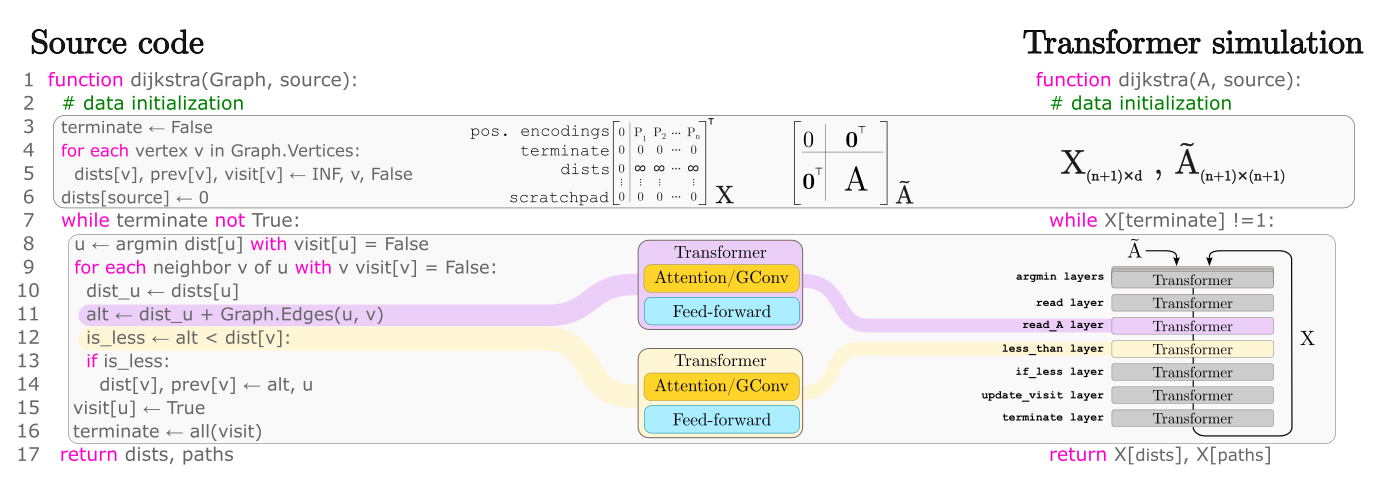
Figure 1: A simplified illustration of the simulation of Dijkstra’s algorithm using a looped transformer with extra attention heads that interact with the graph. On the left, we display the pseudocode of Dijkstra’s algorithm, serving as the source code. The rightmost section shows the corresponding simulation via a transformer, where each step of the source code in the loop is simulated using one or more transformer blocks. We specifically focus on lines 11 and 12, highlighted to demonstrate the simulation of individual functions, as discussed in Section 5. At the top center of the figure, the encoding of graph information and variable scopes into $\tilde{A}$ and $X$ is depicted. For clarity, $X$ is shown in its transposed format. Throughout the transformer loop, $\tilde{A}$ remains constant, while $X$ is updated in each iteration until the simulation meets its termination criteria. Upon termination, the decoding step extracts columns from $X$ that correspond to the algorithm’s desired output.

2 Related work

Empirical: A plethora of papers have been published on the ability of neural networks to execute algorithms on graphs. Representative empirical works are Tang et al. (2020); Yan et al. (2020); Veličković et al. (2020); Ibarz et al. (2022); Bevilacqua et al. (2023); Numeroso et al. (2023); Diao and Loynd (2023); Georgiev et al. (2023a, b); Engelmayer et al. (2023). The authors in these papers utilize the looping mechanism and report favorable scale-generalization results. We refer the reader to Cappart et al. (2023) for a comprehensive review of the subject.

Theoretical: Currently, three types of complementary results study the ability of neural networks to execute algorithms. The first type is simulation results using looped transformers by Pérez et al. (2021); Giannou et al. (2023). These types of results are proved by providing an analytic expression of the neural network which achieves simulation. Our results are also simulation results. In Pérez et al. (2021) the authors prove that the basic transformer architecture is Turing Complete. The authors in Giannou et al. (2023) provide a distinct result of Turing Completeness for transformers. Instead of direct simulation of a Turing Machine, their result is proven through simulation of SUBLEQ Mavaddat and Parhami (1988). Both papers do not take into account graph data. Although these Turing Completeness results apply to graph algorithms as well, their approach requires the graph to be stored in the input data matrix as opposed to having it as part of the architecture. This imposes limitations on the size of the input graph, see Section 4.

The second type of result is using the Probably Approximate Correct learning framework to study the sample complexity of neural networks for executing algorithms. In Xu et al. (2020) the authors show that sample complexity is improved when the neural network is aligned with the structure of the algorithm. We also use the concept of alignment in our constructive proofs. However, our results are about the simulation of algorithms, which hold for any distribution of the test graph. Also, in Xu et al. (2020) they don’t use a looping mechanism. The third type is impossibility results. In this case, it is shown that neural networks can’t execute certain algorithms when the depth and width of the network are smaller than a lower bound. In Loukas (2020) the author studies the ability of graph neural networks to solve various graph problems and also proves Turing Completeness. However, all results are limited by the depth and the width of the neural network which scales with the size of the input graph. In our case, due to the looping mechanism, the depth and width of the network are constant, and a single neural network can solve a particular problem for any input graph, subject to limitations imposed by finite precision.

3 Preliminaries

This section establishes preliminaries for our task of algorithmic simulation on graphs. Recognizing that an algorithm consists of multiple steps, we start by defining simulation for an individual step. Consider $h_{F}:\mathcal{X}\rightarrow\mathcal{Y}$ as the function we aim to simulate and $h_{T}:\mathcal{X^{\prime}}\rightarrow\mathcal{Y^{\prime}}$ as the neural network designed for this purpose. Note that $h_{F}$ and $h_{T}$ might operate in different representation spaces. For instance, $\mathcal{X}$ and $\mathcal{Y}$ might be the set of natural numbers while $\mathcal{X^{\prime}}$ and $\mathcal{Y^{\prime}}$ might be multidimensional reals. To address this, we use mappings $g_{e}:\mathcal{X}\rightarrow\mathcal{X^{\prime}}$ and $g_{d}:\mathcal{Y^{\prime}}\rightarrow\mathcal{Y}$ for encoding and decoding, respectively. In our constructions in Section 5.1, $g_{e}$ organizes terms into our input matrix format and incorporates biases and positional encodings, while $g_{d}$ simply extracts the appropriate columns from the output.

Definition 3.1 (Simulation).

The neural network $h_{T}$ is a successful simulator of the algorithmic step $h_{F}$ if for every input $x\in\mathcal{X}$, $h_{F}(x)=g_{d}(h_{T}(g_{e}(x)))$. A transformer is said to simulate an algorithm if it can simulate each step of the algorithm (Giannou et al., 2023; Pérez et al., 2021).

We define a graph $G$ with $n$ nodes by its adjacency matrix $A\in\mathbb{R}_{+}^{n\times n}$, where $A_{i,j}>0$ if nodes $i$ and $j$ are connected, otherwise $A_{i,j}$ is zero. In our work, we also use an input matrix $X\in\mathbb{R}^{K\times d}$, where $d$ is the feature dimension and $K\geq n+1$ is the number of rows that are set according to the simulation. The structure of $X$ is further explained in Section 5.1. Because of the mismatch of length between $X$ and $A$, we adopt a padded version of $A$, denoted $\tilde{A}\in\mathbb{R}^{K\times K}$. The entries of the first row and column of $\tilde{A}$ are set to zero. This is to align with the input’s top row, which holds data not associated with any node, as further discussed in Section 5.1. The next $n$ rows and columns correspond to the entries of $A$. Certain implementations require $K>n+1$. In this case, we further pad $\tilde{A}$ with zeros in the extra rows and columns beyond the entries of $A$. For example, in our Turing Completeness result in Remark 6.5, $K$ can exceed $n+1$ because the number of rows may not be directly determined by the number of nodes.

4 The Architecture

We utilize a variation of the standard transformer layer in Vaswani et al. (2017) with an additional attention mechanism that incorporates the adjacency matrix. The additional attention mechanism is described by the following equation:

$$\psi^{(i)}(X,\tilde{A}):=\tilde{A}\,\sigma\!\left(XW^{(i)}_{Q}{W^{(i)}_{K}}^{\top}X^{\top}\right)XW^{(i)}_{V},$$ (1)

where $W_{V}\in\mathbb{R}^{d\times d}$, $W_{Q}$, and $W_{K}\in\mathbb{R}^{d\times d_{a}}$ are the value, query, and key matrices, respectively, $d_{a}$ represents the embedding dimension and $\sigma$ denotes the hardmax function. Note that setting $\tilde{A}$ as the identity matrix reduces equation (1) to a standard attention head. This modification efficiently extracts specific rows from matrix $A$. Conversely, applying attention to the transpose of $\tilde{A}$ enables the extraction of columns of $A$. These variations are important in our constructions, and they allow parallel execution of algorithmic subroutines which are further discussed in Section 5.2. We define a complete transformer layer as:

$$f(X,\tilde{A})=f_{\textrm{mlp}}(f_{\textrm{attn}}(X,\tilde{A}))$$ (2)

where

$$f_{\textrm{attn}}(X,\tilde{A})=X+\sum_{i\in H}\!\psi^{(i)}(X,I_{n+1})+\sum_{i\in H_{A}}\!\psi^{(i)}(X,\tilde{A})+\sum_{i\in H_{A^{\top}}}\!\psi^{(i)}(X,\tilde{A}^{\top})$$

$$f_{\textrm{mlp}}(X)=Z^{(m)}W^{(m)}+X,\ \ Z^{(j+1)}=\phi(Z^{(j)}W^{(j)})$$

for $j=0,\dots,m-1$ and $Z^{(0)}=X$. Here, $X$ represents the input matrix and $\tilde{A}$ is the padded adjacency matrix. Additionally, $I_{n+1}$ is the identity matrix of size $n+1$, $m$ and $\phi$ are the number of layers and activation function of $f_{\text{MLP}}$, respectively. Note that in the formulation of the multi-head attention, we adopt a residual connection and a sum of attention heads $\psi$ in the format described in (2). $H$, $H_{A}$, and $H_{A^{\top}}$ are the index set of attention heads for the standard attention Vaswani et al. (2017), as well as for the versions that utilize the adjacency matrix and its transpose, respectively. The total number of attention heads is $\left|H\right|+\left|H_{A}\right|+\left|H_{A^{\top}}\right|$. Furthermore, for the Multilayer Perceptron (MLP), we define $\phi$ to be the ReLU function, we set $m=4$, and we use matrices $W^{(i)}\in\mathbb{R}^{d\times d}$ as the parameters of the MLP, where $d$ is the feature dimension of $X$. We integrate the bias into the linear operations by adding bias columns to $X$ and also introduce a residual connection to $f_{\text{mlp}}$.

Algorithm 1 demonstrates the use of our model $h_{T}$, which is constructed by stacking multiple layers as depicted in (2). In this setting, each forward pass feeds its output to a subsequent pass, creating a looping mechanism. This loop continues until a pre-defined termination condition is met, such as the activation of a boolean element within the input, denoted by term in Algorithm 1. This setting and architecture are used to simulate various graph algorithms, as formally established in the results of Section 6.

Algorithm 1 Looped Transformer Giannou et al. (2023)

0:  Input: model $h_{T}$, matrices $X$ and $\tilde{A}$, column term

1:  while X[0,term] is false do

2:     $X=h_{T}(X,\tilde{A})$

3:  end while

4.1 Discussion on the attention head in (1)

While encoding the graph in $X$ is an alternative to our attention head in (1), it is subject to limitations. Specifically, concatenating the adjacency matrix to $X$ results in linear dependence of the width of the network to the number of nodes, thereby limiting simulation to graphs with sizes smaller or equal to the one that the network was set up/trained on. Alternatively, appending the edges of the graph to the input results in the number of positional encodings being dependent on the edge count, which may increase quadratically as the number of nodes grows. This can limit simulation performance when the available positional encodings are limited, for instance, due to finite precision.

Finally, our attention head in (1) can be viewed as a message-passing layer that performs two convolutions. The first convolution corresponds to a complete graph, i.e., standard attention (Vaswani et al., 2017), and the second is a standard graph convolution (Kipf and Welling, 2017). Multiplying the two convolution matrices is important. In particular, the left multiplication of the attention matrix with $\tilde{A}$ in (1) allows for direct and easy access to data from $\tilde{A}$. This is because the attention matrix acts as an indicator matrix that extracts rows from $\tilde{A}$, see Section 5.3 for details. Note that our attention head in (1) differs from Graph Attention Networks (GAT) Veličković et al. (2018), where the graph is incorporated in the attention mechanism. Although possible to use the attention mechanism in GAT to access the graph data, the proofs will be more elaborate than with (1).

5 Simulation Details

Our simulation results are constructive. We set the parameters of the layer in (2) such that we simulate each sub-routine within each algorithm. We start by describing the input to the model in Section 5.1. We provide two simulation examples of common subroutines among all algorithms in this paper. In Section 5.2 we provide an example of the implementation of the less-than function. This function is common among algorithms in this paper, and it illustrates how the neural network can achieve parallel computation over the nodes. Next, in Section 5.3 we provide an example for reading information from the graph. Throughout the section, we use Dijkstra’s algorithm as an algorithm example (as depicted in Figure 1). With the exemption of our Turing Completeness result in Remark 6.5, it is sufficient to set $K=n+1$ for all algorithms in our paper. For this reason, and for simplicity, we set $K=n+1$ in this section.

5.1 Input matrix

The input matrix encompasses all variables used in the algorithm. In the case of Dijkstra’s algorithm in Figure 1, the lists of current distances and paths (dists and paths), and variables like the current node and its distance (u and dist) are all incorporated into $X$. Below, we describe in detail the general structure of $X$. We refer the reader to Figure 2 for a visualization of the structure of the matrix $X$.

The top row of $X$ stores single variables, encapsulating the global information relevant to the algorithm. The bottom $n$ rows of $X$ are reserved for local variables, such as distances and paths, representing the node-specific data. This storage structure separates the global context from the more specific, node-related information of the algorithm. The input matrix $X$ is augmented with columns for positional encodings, biases, and a scratchpad area. Each node receives a unique positional encoding, denoted by $p_{i}$. These concepts have been present in various contexts, see Giannou et al. (2023) for assigning functional blocks to the input and Akyürek et al. (2022); Wei et al. (2022a); Giannou et al. (2023) for the notion of scratch space. Distinct biases are applied to the top and bottom rows to simulate global and local functions effectively. $X$ is equipped with flags indicating global or local states, regulating the algorithm’s flow. These flags can either permit or prevent overwriting of fields or signal different stages in the algorithm’s execution. For example, in all our simulations each of the last $n$ entries of the node-wise flag named visit indicates whether the corresponding node has been visited, while the global variable term, signals the terminating condition for the algorithm. Finally, the scratchpad within $X$ serves as a temporary storage space for variable manipulation or intermediate computations.

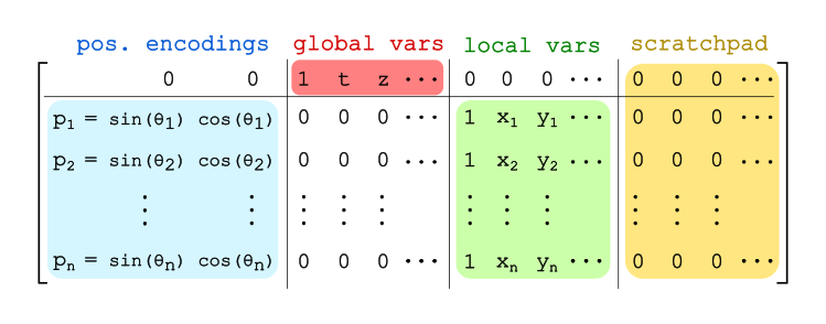
Figure 2: Illustration of the input structure used in the simulation of graph algorithms. On the left, columns indicate node positions using circular positional encodings Liu et al. (2023), detailed in Section 6. The next blocks on the right denote the global (in red) and local (in green) variables, which occupy the top and last $n$ rows of $X$, respectively. In these blocks, the first column marks the bias of the corresponding variables. The symbol $t$ indicates the termination flag, while symbols $z$, and $x_{i},y_{i}$, are generic local and global variables, respectively. Finally, depicted in the far right block, the scratchpad is used for temporary storage and calculation. Non-shaded areas remain null during execution.

5.2 Less-than

The purpose of this operation is to determine whether each element in a specific column of $X$ is smaller than its counterpart in another column. The result of this comparison is then recorded in another designated column. In the context of Dijkstra’s algorithm, as shown in Figure 1, this function plays a critical role in determining if an alternate path is shorter than the shortest path currently known.

We express this function as: less-than(X, C, D, E) = write(X[:,C] < X[:,D], X[:,E]). Here, $X$ is the input matrix, while $C$, $D$, and $E$ are placeholders for the specified column indices in $X$. This simulation involves two key steps. First, we approximate the less-than operator ($<$) using the following expression:

$$X[:,C]<X[:,D]\approx\>\varepsilon^{-1}\left(\phi\left(X[:,D]-X[:,C]\right)-\phi\left(X[:,D]-X[:,C]-\varepsilon\right)\right),$$

where $\varepsilon>0$ is a small tolerance value, and $\phi$ denotes the ReLU activation function. This operation approximates a step function of the difference X[:,C]-X[:,D], where $\varepsilon$ controls the sharpness of the threshold. If this difference is larger than $\varepsilon$, the subtraction of the terms post-ReLU equals $\varepsilon$, which simplifies to $1$. If the difference is negative, both ReLU terms become zero. If the difference X[:,C]-X[:,D] is non-negative but less than $\varepsilon$, the approximation linearly interpolates between 0 and 1, with a gradient of $\varepsilon^{-1}$. The second operation is the write function. In this operation, the output of the less-than comparison is placed in the specified field, while the original content of that field is erased. This operation is expressed as: X[:,E]$\,\leftarrow\,$X[:,E] - X[:,E] + X[:,S₁], where S₁ is the scratchpad column that holds the result to be put in E.

Combining these two operations, we define the parameters for the layer $f$. To understand the purpose behind each operation, we start by defining a particular instance of the matrix $X$, which is used for this example:

$$X=\mathop{\left[\begin{array}[]{ccccccc}\displaystyle\smash{\mathop{\mathinner{\cdotp\mkern-2.0mu\cdotp\mkern-2.0mu\cdotp}}^{\raisebox{6.0pt}{\scriptsize}}}&\displaystyle\smash{\mathop{1}^{\raisebox{6.0pt}{\scriptsize$B_{\text{global}}$}}}&\displaystyle\smash{\mathop{0}^{\raisebox{6.0pt}{\scriptsize$B_{\text{local}}$}}}&\displaystyle\smash{\mathop{c_{0}}^{\raisebox{6.0pt}{\scriptsize\raisebox{1.33002pt}{$C$}}}}&\displaystyle\smash{\mathop{d_{0}}^{\raisebox{6.0pt}{\scriptsize\raisebox{-1.39998pt}{$D$}}}}&\displaystyle\smash{\mathop{e_{0}}^{\raisebox{6.0pt}{\scriptsize\raisebox{1.25995pt}{$E$}}}}&\displaystyle\smash{\mathop{\mathinner{\cdotp\mkern-2.0mu\cdotp\mkern-2.0mu\cdotp}}^{\raisebox{6.0pt}{\scriptsize\raisebox{1.25995pt}{$S$}}}}\\ \hline\cr\mathinner{\cdotp\mkern-2.0mu\cdotp\mkern-2.0mu\cdotp}&0&1&c_{1}&d_{1}&e_{1}&\mathinner{\cdotp\mkern-2.0mu\cdotp\mkern-2.0mu\cdotp}\\ &\vdots&\vdots&\vdots&\vdots&\vdots&\\ \mathinner{\cdotp\mkern-2.0mu\cdotp\mkern-2.0mu\cdotp}&0&1&c_{n}&d_{n}&e_{n}&\mathinner{\cdotp\mkern-2.0mu\cdotp\mkern-2.0mu\cdotp}\\ \end{array}\right].}$$

Here, $C$, $D$ and $E$ are placeholders for column indices used in (5.2), $S$ is the scratchpad area, and $B_{\text{global}}$ and $B_{\text{local}}$ represent the biases for global and local variables respectively. First, in the definition of the attention layer, all values are set to 0, maintaining only the residual connection. For the definition of the parameters in $f_{\text{mlp}}$, we introduce the parameters layer by layer, followed by an explanation of what is achieved at each stage. For the first layer, we have:

$$(W^{(1)})_{i,j}=\begin{cases}1&\text{if }(i,j\!=\!E)\,\text{or}\,(i=D,j\in\{S_{1},S_{2}\})\\ -1&\text{if }i=C,\;j\in\{S_{1},S_{2}\}\\ -\varepsilon&\text{if }i\in\{B_{\text{global}},B_{\text{local}}\},\;j=S_{2}\\ 0&\text{otherwise,}\end{cases}$$

where $S_{1}$ and $S_{2}$ are entries in the scratchpad. Here, the parameters of the first layer $W^{(1)}$ keep the entries of the target column $E$, while it builds the arguments of $\phi$ in (5.2), inserting them in the scratchpad. Storing the intermediate values in the scratchpad is beneficial to prevent overwriting issues, as it avoids the use of columns involved in the definition of the equation. The result is given by:

$$XW^{(1)}\!=\!{\mathop{\left[\begin{array}[]{ccccc}\displaystyle\smash{\mathop{\mathinner{\cdotp\mkern-2.0mu\cdotp\mkern-2.0mu\cdotp}}^{\raisebox{6.0pt}{\scriptsize}}}&\displaystyle\smash{\mathop{e_{0}}^{\raisebox{6.0pt}{\scriptsize\raisebox{2.58997pt}{$E$}}}}&\displaystyle\smash{\mathop{d_{0}-c_{0}}^{\raisebox{6.0pt}{\scriptsize$S_{1}$}}}&\displaystyle\smash{\mathop{d_{0}-c_{0}-\varepsilon}^{\raisebox{6.0pt}{\scriptsize$S_{2}$}}}&\displaystyle\smash{\mathop{\mathinner{\cdotp\mkern-2.0mu\cdotp\mkern-2.0mu\cdotp}}^{\raisebox{6.0pt}{\scriptsize}}}\\ \hline\cr\mathinner{\cdotp\mkern-2.0mu\cdotp\mkern-2.0mu\cdotp}&e_{1}&d_{1}-c_{1}&d_{1}-c_{1}-\varepsilon&\mathinner{\cdotp\mkern-2.0mu\cdotp\mkern-2.0mu\cdotp}\\ &\vdots&\vdots&\vdots&\\ \mathinner{\cdotp\mkern-2.0mu\cdotp\mkern-2.0mu\cdotp}&e_{n}&d_{n}-c_{n}&d_{n}-c_{n}-\varepsilon&\mathinner{\cdotp\mkern-2.0mu\cdotp\mkern-2.0mu\cdotp}\end{array}\right].}}$$

Subsequently, the parameters of the second layer $W^{(2)}$ are:

$$(W^{(2)})_{i,j}=\begin{cases}1&\text{if }i=E,\;j=i\\ \varepsilon^{-1}&\text{if }i=S_{1},\;j=i\\ -\varepsilon^{-1}&\text{if }i=S_{2},\;j=S_{1}\\ 0&\text{otherwise.}\end{cases}$$

Here, $W^{(2)}$ is responsible for subtracting the post-ReLU terms and dividing them by $\varepsilon^{-1}$. This result is then stored in the scratchpad entry $S_{1}$:

$$Z^{(1)}W^{(2)}\approx\!\mathop{\left[\begin{array}[]{cccc}\displaystyle\smash{\mathop{\mathinner{\cdotp\mkern-2.0mu\cdotp\mkern-2.0mu\cdotp}}^{\raisebox{6.0pt}{\scriptsize}}}&\displaystyle\smash{\mathop{e_{0}}^{\raisebox{6.0pt}{\scriptsize\raisebox{2.58997pt}{$E$}}}}&\displaystyle\smash{\mathop{c_{0}<d_{0}}^{\raisebox{6.0pt}{\scriptsize$S_{1}$}}}&\displaystyle\smash{\mathop{\mathinner{\cdotp\mkern-2.0mu\cdotp\mkern-2.0mu\cdotp}}^{\raisebox{6.0pt}{\scriptsize}}}\\ \hline\cr\mathinner{\cdotp\mkern-2.0mu\cdotp\mkern-2.0mu\cdotp}&e_{1}&c_{1}<d_{1}&\mathinner{\cdotp\mkern-2.0mu\cdotp\mkern-2.0mu\cdotp}\\ &\vdots&\vdots&\\ \mathinner{\cdotp\mkern-2.0mu\cdotp\mkern-2.0mu\cdotp}&e_{n}&c_{n}<d_{n}&\mathinner{\cdotp\mkern-2.0mu\cdotp\mkern-2.0mu\cdotp}\\ \end{array}\right].}$$

Finally, for the two remaining operations, we have:

$$(W^{(3)})_{i,j} =\begin{cases}1&\text{if }i\in\{E,S_{1}\},\;j=i\\ 0&\text{otherwise,}\end{cases}$$

$$(W^{(4)})_{i,j} =\begin{cases}-1&\text{if }i,j=E\\ 1&\text{if }i=S_{1},\;j=E\\ 0&\text{otherwise.}\end{cases}$$

In these two operations, the output of $S_{1}$ is preserved and then placed in the desired field $E$. Additionally, the entries of $E$, which were kept in the first three layers, are subtracted from the target field in $W^{(4)}$, effectively removing the previous entry in $E$. Furthermore, to address cases where the input entries are negative, it is necessary to incorporate additional parameters. These parameters should follow the same structure as previously provided, with inverted signs in the parameters $W^{(1)}$ and $W^{(4)}$ for columns $C$, $D$, and $E$. These additional entries are generally placed in the scratchpad.

Parallel computation over the nodes: The node-wise format in Section 5.1 is particularly beneficial for operations like less-than in equation (5.2) because it operates across entire columns. This approach enables parallel processing for all nodes in a graph, enhancing efficiency in algorithms. For example, in Dijkstra’s algorithm, the typical implementation involves iterating through each non-visited neighbor of a node. However, by integrating an additional masking function, we can filter out visited or non-neighboring nodes. This allows us to conduct all necessary comparisons and conditional selections for every node simultaneously within the inner loop of the implementation. This modification enhances the algorithm’s efficiency by reducing the need for repetitive looping in transformer-based simulations.

5.3 Read row from $A$

In this section, we provide a configuration of (2) that extracts a row from the adjacency matrix. We describe the function as read-A(X, Ã, C, D) = write(Ã[C,:], X[:,D]), where $X$ and $\tilde{A}$ are the input and padded adjacency matrices, while $C$ and $D$ are the row and column indices for the respective matrices. The input structure for this operation requires specialized inputs common to all algorithms presented in this work. This includes a set of columns to store the node-wise positional encodings, denoted as $P$. Additionally, a global variable representing the positional encoding of the node of interest is stored in a distinct set of columns, marked as $P_{\text{cur}}$. The structure of the input matrix $X$ is given below:

$$X=\mathop{\left[\begin{array}[]{cccccccc}\displaystyle\smash{\mathop{\mathinner{\cdotp\mkern-2.0mu\cdotp\mkern-2.0mu\cdotp}}^{\raisebox{6.0pt}{\scriptsize}}}&\displaystyle\smash{\mathop{0}^{\raisebox{6.0pt}{\scriptsize$P$}}}&\displaystyle\smash{\mathop{p_{i}}^{\raisebox{6.0pt}{\scriptsize\raisebox{1.33002pt}{$P_{\text{cur}}$}}}}&\displaystyle\smash{\mathop{1}^{\raisebox{6.0pt}{\scriptsize$B_{\text{global}}$}}}&\displaystyle\smash{\mathop{0}^{\raisebox{6.0pt}{\scriptsize$B_{\text{local}}$}}}&\displaystyle\smash{\mathop{c_{0}}^{\raisebox{6.0pt}{\scriptsize\raisebox{1.33002pt}{$C$}}}}&\displaystyle\smash{\mathop{d_{0}}^{\raisebox{6.0pt}{\scriptsize\raisebox{-1.33002pt}{$D$}}}}&\displaystyle\smash{\mathop{\mathinner{\cdotp\mkern-2.0mu\cdotp\mkern-2.0mu\cdotp}}^{\raisebox{6.0pt}{\scriptsize\raisebox{1.33002pt}{$S$}}}}\\ \hline\cr\mathinner{\cdotp\mkern-2.0mu\cdotp\mkern-2.0mu\cdotp}&p_{1}&0&0&1&c_{1}&d_{1}&\mathinner{\cdotp\mkern-2.0mu\cdotp\mkern-2.0mu\cdotp}\\ &\vdots&\vdots&\vdots&\vdots&\vdots&\vdots&\\ \mathinner{\cdotp\mkern-2.0mu\cdotp\mkern-2.0mu\cdotp}&p_{n}&0&0&0&c_{n}&d_{n}&\mathinner{\cdotp\mkern-2.0mu\cdotp\mkern-2.0mu\cdotp}\\ \end{array}\right].}$$

For simplicity, we let the embedding dimension $d_{a}=2$, which corresponds to the dimension of positional encodings. For the attention head for $\tilde{A}$ in (2), we define:

$$(W_{K},W_{Q})_{i,j} =\begin{cases}1&\text{if }i\in\{(P)_{j},(P_{\text{cur}})_{j}\},\;j=1,2\\ 0&\text{otherwise,}\end{cases}$$

$$(W_{V})_{i,j} =\begin{cases}2&\text{if }i=B_{\text{global}},j=D\\ 0&\text{otherwise.}\end{cases}$$

The multiplication $XW_{Q}W^{\top}_{K}X^{\top}$ results in a matrix where each element is the inner product between positional encodings of nodes. Positional encodings are formulated such that $\left<p_{i},p_{i}\right>>\left<p_{i},p_{j}\right>$ whenever $i\neq j$ for $i,j\in[n]$. By leveraging this property, we allow the attention matrix to behave as an indicator function. The result is given below:

$$\small\sigma\!\left(XW_{Q}W^{\top}_{K}X^{\top}\right)={\tiny\left[\begin{array}[]{c|cccc}\nicefrac{{1}}{{2}}&0&\mathinner{\cdotp\mkern-2.0mu\cdotp\mkern-2.0mu\cdotp}&\nicefrac{{1}}{{2}}&\mathinner{\cdotp\mkern-2.0mu\cdotp\mkern-2.0mu\cdotp}\\ \hline\cr 0&1&\mathinner{\cdotp\mkern-2.0mu\cdotp\mkern-2.0mu\cdotp}&0&\mathinner{\cdotp\mkern-2.0mu\cdotp\mkern-2.0mu\cdotp}\\ \vdots&\vdots&\ddots&\vdots&\\ \nicefrac{{1}}{{2}}&0&\mathinner{\cdotp\mkern-2.0mu\cdotp\mkern-2.0mu\cdotp}&\nicefrac{{1}}{{2}}&\mathinner{\cdotp\mkern-2.0mu\cdotp\mkern-2.0mu\cdotp}\\ \vdots&\vdots&&\vdots&\ddots\\ 0&0&\mathinner{\cdotp\mkern-2.0mu\cdotp\mkern-2.0mu\cdotp}&0&\mathinner{\cdotp\mkern-2.0mu\cdotp\mkern-2.0mu\cdotp}\end{array}\right]}.$$

The result of the multiplication of the attention matrix and $\tilde{A}$ is further multiplied by the input $X$:

$$\small\tilde{A}\,\sigma\!\left(XW_{Q}W^{\top}_{K}X^{\top}\right)X=\nicefrac{{1}}{{2}}{\mathop{\left[\begin{array}[]{ccc}\displaystyle\smash{\mathop{\mathinner{\cdotp\mkern-2.0mu\cdotp\mkern-2.0mu\cdotp}}^{\raisebox{6.0pt}{\scriptsize}}}&\displaystyle\smash{\mathop{0}^{\raisebox{6.0pt}{\scriptsize\tiny$B_{\text{global}}$}}}&\displaystyle\smash{\mathop{\mathinner{\cdotp\mkern-2.0mu\cdotp\mkern-2.0mu\cdotp}}^{\raisebox{6.0pt}{\scriptsize}}}\\ \hline\cr\mathinner{\cdotp\mkern-2.0mu\cdotp\mkern-2.0mu\cdotp}&A_{1i}&\mathinner{\cdotp\mkern-2.0mu\cdotp\mkern-2.0mu\cdotp}\\ &\vdots&\\ \mathinner{\cdotp\mkern-2.0mu\cdotp\mkern-2.0mu\cdotp}&A_{in}&\mathinner{\cdotp\mkern-2.0mu\cdotp\mkern-2.0mu\cdotp}\\ \end{array}\right].}}$$

The result in column $B_{\text{global}}$ is written in the target column $D$ by $W_{V}$. Notice that in this case, the target field must also be erased. This can be done as in Section 5.2, using the $f_{\text{mlp}}$ and an intermediate scratchpad field, or by leveraging another attention head to replicate the identity matrix and subtract the values in the target columns.

6 Theoretical analysis

In this section we demonstrate the ability of the architecture in (2) to simulate various graph algorithms. We provide empirical validation of the results in Section B.3. We discuss the implications of incorporating attention heads in the form of (1) and we demonstrate that the overall architecture is Turing Complete, even when constrained to constant width. We start by describing the positional encodings we use and other related parameters in our architecture.

6.1 Positional encodings and increment

In our approach, we use circular positional encodings to enumerate the nodes in the graph Liu et al. (2023). This enumeration is carried out by discretizing the unit circle into intervals of angle $\hat{\delta}$. Each node is then represented by a tuple of sine and cosine values.

For node enumeration, we use the formula $p_{i}=R^{\top}_{\hat{\delta}}p_{i-1}$ for $i\geq 1$. In this context, $\hat{\delta}$ represents the smallest rotation that our system can represent with limited precision. This parameter essentially sets the limit on the number of nodes we can enumerate, which is capped at $\lfloor 2\pi\hat{\delta}^{-1}\rfloor$. This limit is determined by the precision with which we can represent $\hat{\delta}$, thus influencing the maximum number of distinct nodes that can be effectively encoded. This approach inherently compensates for rotational imprecision since the encodings are generated by the rotation matrix and not by the trigonometric functions of each angle. Although this could affect the periodicity of the function, our designs do not rely on this attribute. What is crucial is that the increment function can be executed by a neural network, and the positional encodings satisfy the condition: $\left<p_{i},p_{i}\right>>\left<p_{i},p_{j}\right>$ for $i\neq j$ (see Section 5.3). The rotation matrix $R_{\hat{\delta}}$ can be efficiently implemented as a single linear layer within $f_{\text{MLP}}$. Furthermore, since $R_{\hat{\delta}}$ has unitary singular values, all positional encodings have unitary norms, thus by the Cauchy-Schwarz Inequality, the inner product property is preserved.

6.2 Maximum absolute value parameter

All algorithms that we simulate utilize a conditional selection function. The implementation of this function depends on the parameter $\Omega$, which represents the maximum absolute value within a clause. We approximate the conditional selection function in the following manner:

$$\texttt{if-else($c_{1},c_{0},\gamma$)}\approx\phi\left(c_{0}-\gamma\,\Omega\right)+\phi\left(c_{1}-\left(1-\gamma\right)\Omega\right),$$

where $c_{0},c_{1}\in[-\Omega,\Omega]$ are the clause values and $\gamma\in\{0,1\}$ is the condition. When $\gamma=0$, the function outputs $c_{0}$, and $c_{1}$ otherwise. The complete construction also replicates the terms for the negative counterparts of the clauses. This approach relies on $\Omega$ to cancel any opposite terms in the conditional selection. Therefore, $\Omega$ determines the largest absolute value present in the clauses, and any element larger than $\Omega$ breaks the simulation.

6.3 Results on simulation of graph algorithms

We now present our results on transformer-based simulations of graph algorithms. We first present the simulation results for Dijkstra’s algorithm on weighted graphs, accompanied by a brief overview of its proof. We then shift our focus to undirected graphs, examining algorithms such as Breadth-First Search, Depth-First Search, and the identification of Strongly Connected Components. Alongside these results, we provide an outline of the proofs for the related theorems. The complete proofs are in the Appendix C.

Theorem 6.1.

There exists a looped-transformer $h_{T}$ in the form of (2), with 17 layers, 3 attention heads, and layer width $O(1)$ that simulates Dijkstra’s shortest path algorithm for weighted graphs with rational edge-weights, up to $O(\hat{\delta}^{-1})$ nodes and graph diameter of $O(\Omega)$.

Proof Overview: Theorem 6.1 is proved by construction. Our proof begins by adapting Dijkstra’s algorithm to fit our looping structure. This involves unrolling any nested operations to fit within a single loop, as described in Algorithm 1. Although these modifications change Dijkstra’s algorithm from its traditional form, they do not alter its core functionality. In conventional programming, loops within the code must be completed before the rest of the code can continue. However, in the absence of additional structures, our unrolling approach would lead to all instructions being executed all at once. This could potentially disrupt the intended sequence of operations. To address this, we also implement binary flags and conditional selections, as explained in (6.2). These mechanisms are vital for ensuring that certain operations only modify data under specific conditions. A key example in our simulations is the minimum function which has $O(n)$ complexity and runs concurrently with the rest of the algorithm. When this function is active, it prevents modifications by other parts of the algorithm. The modifications can resume once the minimum function has been completed, at which point it becomes inactive. Finally, each step of the rewritten algorithm is implemented as a series of transformer layers in the form of (2), accounting for 17 layers, and three attention heads: two standard and one specialized over $A$. Some of the core simulation mechanisms of these functions are extensively discussed in Section 4 and Section 6, demonstrating that most of the constructions are based on previously described principles. Furthermore, Theorem 6.1 is restricted to rational edge weights due to the inherent limitations of finite precision in representing edge values. We reweight the edges to circumvent issues arising from the tolerance $\varepsilon$ of the less-than function (5.2), which may not adequately capture minor path differences. This involves dividing all edge weights by the smallest absolute edge weight. Consequently, this ensures that the minimal non-zero path difference is effectively greater than one. The graph size is bounded by the enumeration constraints of $\hat{\delta}$, as mentioned in Section 6.1. The dependence on the graph diameter is attributed to the maximum distance that can be constructed during the execution of Dijkstra’s algorithm. Given the algorithm’s design, which excludes the consideration of repeating or negative paths, this quantity is determined by the diameter of the weighted graph, which must remain below $\Omega$.

We now present our results for algorithms on unweighted graphs, followed by a collective discussion of their proofs.

Theorem 6.2.

There exists a looped-transformer $h_{T}$ in the form of (2), with 17 layers, 3 attention heads, and layer width $O(1)$ that simulates Breadth-First Search (BFS) for unweighted graphs with up to $\min(O(\hat{\delta}^{-1}),\,O(\Omega))$ nodes.

Theorem 6.3.

There exists a looped-transformer $h_{T}$ in the form of (2), with 15 layers, 3 attention heads, and layer width $O(1)$ that simulates Depth-First Search (DFS) for unweighted graphs with up to $\min(O(\hat{\delta}^{-1}),\,O(\Omega))$ nodes.

Theorem 6.4.

There exists a looped-transformer $h_{T}$ in the form of (2), with 22 layers, 4 attention heads, and layer width $O(1)$ that simulates Kosaraju’s Strongly Connected Components algorithm for unweighted graphs with up to $\min(O(\hat{\delta}^{-1}),\,O(\Omega))$ nodes.

Proof Overview: Our proofs for Theorems 6.2-6.4 also follow a constructive approach. The implementations of breadth-first and depth-first search are comparable to Dijkstra’s algorithm in terms of the number of layers and attention heads. However, the Strongly Connected Components algorithm utilizes significantly more layers and an additional attention head for $A$, due to its complexity and the need for a depth-first search over both $A$ and $A^{\top}$. Despite the absence of edge weights, we encounter an additional bound of $O(\Omega)$ on the number of nodes. This stems from our method of replicating the behavior of queues and stacks, which are used in these algorithms. Similar to our approach with Dijkstra’s algorithm, we also incorporate an interaction with a minimum function. During the execution of the algorithms, priority values are assigned to the neighbors of each node visited. These assigned values shape the minimum function’s behavior: increasing priority values mimic the functionality of a queue while decreasing values replicate that of a stack. Hence, having more nodes in a graph increases the number of loop iterations, thereby increasing the absolute value of the priority value. Given that these priority values feature in conditional selections, they are also subject to the constraints imposed by $\Omega$. Consequently, the graph’s size limitations are independently determined by either $\hat{\delta}$ or $\Omega$. In the implementation of Breadth-First Search (BFS) and Depth-First Search (DFS), since nodes only need to be visited once, $\Omega$ is the maximum node count for which accurate simulation of any graph is guaranteed. In the implementation of the Strongly Connected Components (SCC) algorithm, which involves two distinct DFS operations, the maximum node count is constrained to $\Omega/3$. This specific limit arises from the two-phase process, and also the role of the first DFS in organizing nodes by their finishing times, which is further detailed in Appendix C.

While our guarantees are limited by parameters $\varepsilon$, $\Omega$, and $\hat{\delta}$, an important question remains: What are the implications of using a graph that fails to meet assumptions in our theorems? This situation could result in inaccurate simulation outcomes or even a failure to meet the pre-established termination condition, thus failing to halt as expected.

6.4 Turing Completeness

We now present our result on Turing Completeness of the architecture in (2). It’s important to note that using a graph convolution operation within the attention mechanism as shown in (1) might affect the model’s expressiveness. We demonstrate that a transformer based on this structure is also Turing Complete. Following the methodology of Giannou et al. (2023), we demonstrate this claim by successfully simulating SUBLEQ, a single-instruction language that, with arbitrary memory resources, is proven to be Turing Complete Mavaddat and Parhami (1988).

Remark 6.5.

There exists a looped-transformer $h_{T}$ in the form of (2), which utilizes the modified attention head in (1), with 11 layers, 3 attention heads, and layer width $O(1)$ that simulates the SUBLEQ.

Proof Overview: We prove that the architecture in (2) simulates a modified version of SUBLEQ, which is also Turing Complete. This modification changes the memory structure of SUBLEQ, utilizing two memory blocks instead of one. The first block is the standard memory block as in Mavaddat and Parhami (1988) which can be read and altered. The second is a special read-only memory that only stores the adjacency matrix. We introduce this memory modification to reflect the fact that the architecture in (2) has two inputs, the data matrix $X$ and the padded adjacency matrix $\tilde{A}$. The former is modified at each iteration of the looped transformer architecture, while the latter is only used in the convolution stage, and it never changes. The modified version of SUBLEQ utilizes data from the graph by reading the data from the second block and copying them to the first block. We show that this operation of reading and copying data can be simulated by our read operation in Section 5.3. The rest of SUBLEQ can be simulated using generic attention heads and MLPs similarly to Giannou et al. (2023). The complete proof is provided in Appendix C.

7 Conclusion and Future Work

We present a constructive approach where a looped transformer, combined with graph convolution operations, is used to simulate various graph algorithms. This demonstrates the potential of looped transformers for algorithmic reasoning on graphs. This architecture also proves to be efficient, as it has constant network width regardless of the input graph’s size, allowing it to handle graphs of varying dimensions.

Currently, in our results, we use a single architecture to simulate various graph algorithms. However, each algorithm is simulated using different parameters in the architecture. We believe that it is possible to have a single neural network that simulates all algorithms. Such a result will be more aligned with the generalist approach in Ibarz et al. (2022). We leave this goal for future work.

Outside the scope of simulation, studying looped transformers for graph algorithms within the Probably Approximate Correct (PAC) learning framework offers an exciting research direction. Specifically, the constructive parameters $\Omega$, $\hat{\delta}$, and $\varepsilon$ are essential in determining which graphs can be simulated. However, these parameters may also influence the learnability of algorithmic subroutines. An interesting research question involves determining the sample complexity of subroutines as a function of these constructive parameters. Investigating this could further reveal the relationship between the design of solutions and their learning effectiveness under the PAC framework.

8 Acknowledgments

K. Fountoulakis would like to acknowledge the support of the Natural Sciences and Engineering Research Council of Canada (NSERC), [RGPIN-2019-04067, DGECR-2019-00147].

Cette recherche a été financée par le Conseil de recherches en sciences naturelles et en génie du Canada (CRSNG), [RGPIN-2019-04067, DGECR-2019-00147].

Appendix A Additional related work

The importance of recurrence in the expressive power of neural networks has been well-established, as evidenced by the Turing Completeness results of Recurrent Neural Networks Siegelmann and Sontag [1995]. Prior to the emergence of transformers, pioneering models like Neural Turing Machines (NTMs) Graves et al. [2014], utilized the idea of recurrence, integrating neural networks with external memory, demonstrating strong performance in tasks such as copying and sorting. Subsequent advances were seen by adapting NTMs for learning algorithmic tasks Kaiser and Sutskever [2016], incorporating a dynamic memory Graves et al. [2016], and utilizing recurrent models to learn multiple programs Reed and De Freitas [2016]. All these advancements laid the groundwork for concepts utilized in transformers and in this work, such as the addressing mechanism of Graves et al. [2014] which shares a similar principle to attention in transformers, and concepts like scratch space for intermediate computations as proposed by Reed and De Freitas [2016].

In the more recent developments related to algorithmic reasoning in transformers, dedicated frameworks have emerged to represent and execute complex algorithmic tasks. An example of this is the Restricted Access Sequence Processing Language (RASP). RASP allows for the expression of sequences of steps in transformers and can be applied to tasks such as token counting and sorting. Along this line, Lindner et al. [2023] developed a compiler for translating between RASP and Transformer models, while Friedman et al. [2023] have designed modified Transformers that can be trained and subsequently converted to RASP instructions.

Appendix B Implementation details

In this section, we describe aspects of the implementation and empirical verification of our simulations. As mentioned in Section 4, despite our constructions being based on hardmax, for the purpose of empirical validation and to better align with the implementation practices in transformers, we utilize the softmax function:

$$\sigma_{S}(z_{i})=\frac{e^{z_{i}}}{\sum_{j=1}^{K}e^{z_{j}}},$$

where $K$ represents the number of elements. When using the softmax in attention, we divide all parameters in $W_{Q}$ and $W_{K}$ by a temperature parameter $T$. The value of $T$ is important as it determines the sharpness of the softmax operation. As shown in Giannou et al. [2023] and Liu et al. [2023], as the temperature gets arbitrarily small, the behavior of the softmax approximates that of the hardmax, which is used in our constructions.

However, it is important to acknowledge that in practice the simulation of all algorithmic steps is subject to numerical limitations due to floating-point arithmetic. For example, using the minimum angle $\hat{\delta}$ that a computer can represent accurately is impractical. The reason is that this quantity becomes overshadowed by subsequent operations that introduce imprecision, such as matrix multiplications, and by non-linear elements like the softmax function in the attention stage. In algorithmic tasks, simulations exhibit a very low tolerance for computational errors. If not properly managed, these errors can propagate, leading to inaccurate prediction or non-termination. To address this, we adopt a more conservative approach in setting parameters for $\hat{\delta}$ and $\varepsilon$ as described in Section B.3. In addition, we incorporate rounding operations for both binary values and positional encodings, following the structure described in (2).

B.1 Rounding functions

We utilize rounding functions in-between the simulated algorithmic steps to ensure that the computation of binary values made by the transformer does not include additional errors that propagate along the simulation. To this end, we adapt the rounding operation presented by Giannou et al. [2023], which can be algebraically expressed as:

$$\text{round}(X[:,C])\approx\eta^{-1}\left(\phi(X[:,C]-\nicefrac{{1}}{{2}})-\phi(X[:,C]-(\nicefrac{{1}}{{2}}+\eta))\right),$$ (3)

where $\eta$ is a small tolerance value. This implementation can also be done using the structure presented in (2), noting that the expression in (3) is equivalent to the less-than function presented in Section 5.2, with $\varepsilon=\eta$, and $X[:,D]$ equivalent to the quantity $1/2$.

In practice, the increment function described in Section C.1.2 introduces noise in the positional encodings. To counter this, we employ a rounding procedure for circular positional encodings. This involves using two transformer layers. The first layer generates a binary vector based on the current positional encoding We then round this quantity utilizing the procedure described in (3), and finally obtain the corresponding positional encoding based on the index position using the last layer.

The first attention layer is set up as described in (6), where $D$ is set to $B_{\text{global}}$, and $S_{\text{PE}}$ denotes the target column in the scratchpad. Another attention head is used to clear the original scratchpad contents, as detailed in (7). The corresponding $f_{\text{MLP}}$ in this layer implements Equation 3, with $S_{\text{PE}}$ as the source column $C$.

In the second transformer layer, the matrices $W^{(1)}_{K}$, $W^{(1)}_{Q}$, and $W^{(1)}_{V}$ of the first attention head are defined as follows:

$$(W^{(1)}_{K},W^{(1)}_{Q})_{i,j}=\begin{cases}\tilde{T}^{\nicefrac{{-1}}{{2}}}&\text{if }i=S_{\text{PE}}\\ 0&\text{otherwise,}\end{cases}\quad(W^{(1)}_{V})_{i,j}=\begin{cases}2&\text{if }i=(P)_{k},j=(E)_{k},\;k\in{0,1}\\ 0&\text{otherwise.}\end{cases}$$

In this layer, $E$ denotes the target columns for inserting positional encodings, and $\tilde{T}$ is an annealed temperature parameter of softmax, which is set higher than in other implementations (e.g., $T=10^{-5}$). This ensures that minor differences in this attention head are minimized, thereby reducing errors in reading positional encodings. Additionally, we use the configuration of (7) in another attention head to clear the contents of $E$ and $S_{\text{PE}}$. Lastly, the implementation of $f_{\text{MLP}}$, as defined in (8), clears the last $n$ entries of the target field $E$.

B.2 Writing prevention after termination

The constructions in the empirical section slightly differ from the ones presented in Appendix C due to an additional consideration. While the theoretical constructions require delivering accurate outputs upon reaching the termination condition, one could continue running the looped transformer after the termination flag is activated. To ensure that the solution is not modified post-termination, we introduce extra constraints in the form of flags that deactivate write permissions once the termination condition is met. These are articulated through algebraic expressions, easily integrating into the transformer implementation. In practice, the writing permission flag is not determined solely by the minimum function’s termination flag (term${}_{\text{min}}$) for the implementation of Theorem 6.1 and similar algorithms. Instead, we construct a flag defined as write = term${}_{\text{min}}$ and (not term), which can be implemented as $\texttt{X[:,write]}=\phi(\texttt{X[:,term${}_{\text{min}}$]-X[:,term]})$. This condition ensures that once the algorithm reaches the termination state, writing is forbidden.

Furthermore, we employ a conditional selection mechanism – as explained in Section C.1.1 – to maintain the termination flag, which is activated if the terminating condition is met but the simulation continues running. This is performed by first moving the calculation of the termination condition to a temporary storage area, denoted as $S_{\text{term}}$. Then, at the end of each iteration, we execute the layer: cond-select(X, S${}_{\text{term}}$, term, S${}_{\text{term}}$, term). This means that if the recalculated termination condition in $S_{\text{term}}$ is true, then the term variable is updated; otherwise, it remains unchanged, effectively managing the looped transformer’s operation post-termination.

B.3 Empirical validation

We validate our theoretical results using graphs in the CLRS Algorithmic Reasoning Benchmark Veličković et al. [2022]. This benchmark offers data created for multiple tasks, including sorting, searching, and geometry, among others. Additionally, it encompasses tasks specific to graphs, including those simulated in this study. These tasks are divided into segments with varying input sizes. For graph-related tasks, the training and validation sets include graphs with 16 nodes, while the test set contains graphs with 64 nodes. In Table 1, we show that our simulations achieve perfect accuracy across all tested instances.

Table 1: Accuracy over algorithmic tasks on CLRS

Split (size)	BFS	DFS	Dijkstra	SCC
Train (1000)	100%	100%	100%	100%
Validation (32)	100%	100%	100%	100%
Test (32)	100%	100%	100%	100%

In our empirical verifications, we consistently apply specific parameters: an angular increment $\delta$ set at $10^{-2}$, a maximum value $\Omega$ of $10^{5}$, and a temperature parameter $T$ at $10^{-7}$. Additionally, in the masking operations such as Section C.2.1, we address numerical imprecision during execution by using a value that is an order of magnitude smaller than $\Omega$. This precaution is crucial because minor inaccuracies that slightly increase these values above $\Omega$ could lead to cumulative errors in the conditional selection function, potentially impacting the integrity of our results.

Furthermore, beyond the practical considerations discussed in the previous sections, the implementation of breadth-first search in the CLRS benchmark slightly differs from the one presented in Algorithm 4. This is because, as mentioned in Veličković et al. [2022], the results of the algorithm are built on top of the concept of parallel execution, which implies that for algorithms such as breadth-first search, there is no concept of order in the discovery of neighbor nodes, as outlined in Cormen et al. [2022]. Instead, the order of discovery in CLRS is established by the value of the node index. Therefore, to address this particularity, the implementation of the conditional selection function in step (9) of Algorithm 4 has another pair of clauses, which can be expressed by cond-select(X, val${}_{\text{best}}$, order, term${}_{\text{min}}$, order). Essentially, this variation in the implementation is designed to capture the priority value from the parent node, thereby ensuring uniform priority assignment across all nodes within the same neighborhood level.

Appendix C Proofs of Theorems

C.1 Preparations for the proofs

In this section, we first introduce key coding primitives that are essential to all the algorithmic simulations presented. We illustrate these coding primitives through the algorithm of the minimum function. This function is designed to identify the smallest value in a list, along with its index and other pertinent information. As outlined in Section 6, for each simulated algorithm, we adapt their formulations to align with the looped architecture of the transformer. Although this architecture inherently does not support inner loops, we simplify the presentation of the pseudocode by using inner loops solely to depict functions that are operated in parallel by the transformer. As further depicted in Algorithms 3-6, the iteration of the minimum function described in Algorithm 2 is executed inside the main loop of the transformer, along with the other functions of the corresponding algorithms. The algorithm description is also accompanied by comments that enumerate the steps that are implemented using the layer formulation in (2). Each comment is also linked to the section that provides a more detailed explanation of its implementation.

Algorithm 2 Iteration of the minimum function (get_minimum)

0:  Input: data $x$, size $n$ List of values to find the minimum

0:  Input: data $x_{\text{SCC}}$, size $n$

1:  scc${}_{\text{cur}}$, scc${}_{\text{best}}$ = 0, 0 Only used for SCC

2:  idx${}_{\text{cur}}$, val${}_{\text{cur}}$ = 0, 0

3:  idx${}_{\text{best}}$, val${}_{\text{best}}$ = 0, $\Omega$

4:  visit${}_{\text{min}}$ = array of size $n$

5:  for $i=1$ to $n$ do

6:    visit${}_{\text{min}}$[i] = false

7:  end for

8:  term${}_{\text{min}}$ = false

9:  if term${}_{\text{min}}$ is true then

10:    $\cdots$

11:    term${}_{\text{min}}$ = false(1) Re-initialize variables [C.1.1]

12:  end if

13:  idx${}_{\text{cur}}$ = idx${}_{\text{cur}}$ + 1 (2) Increment position [C.1.2]

14:  val${}_{\text{cur}}$ = $x$[idx${}_{\text{cur}}$] (3) Read value at current position [C.1.3]

15:  scc${}_{\text{cur}}$ = $x_{\text{SCC}}$[idx${}_{\text{cur}}$]

16:  condition = val${}_{\text{cur}}$ $<$ val${}_{\text{best}}$ (4) Compare values [C.1.4]

17:  if condition then

18:    val${}_{\text{best}}$, idx${}_{\text{best}}$ = val${}_{\text{cur}}$, idx${}_{\text{cur}}$ (5) Update variables [C.1.1]

19:    scc${}_{\text{best}}$ = scc${}_{\text{cur}}$

20:  end if

21:  visit${}_{\text{min}}$[idx${}_{\text{cur}}$] = true(6) Visit current position [C.1.5]

22:  term${}_{\text{min}}$ = not (false in visit${}_{\text{min}}$) (7) Trigger termination [C.1.6]

The lines [1-8] consist of the initialization of the data, while the remaining represent the algorithm executed inside the loop. Note that lines 1, 15, and 19 are highlighted in gray, and are only defined in the case of the Strongly Connected Components algorithm. As described in Section 5.1, the single variables (e.g. val${}_{\text{cur}}$) occupy the top row, while lists (e.g. visit${}_{\text{min}}$) occupy the last $n$ rows of $X$. Furthermore, the implementation of indexes requires two different representations in the input matrix $X$.

In Algorithm 2, these correspond to idx${}_{\text{cur}}$ and idx${}_{\text{best}}$ as well as the variables for the Strongly Connected Component implementation. In $X$, these indices are represented both as integer numbers and positional encodings. The latter is vital for algorithm functionality, while integer numbers are key in the decoding phase, forming the output data. Consequently, ambiguous variables in proofs are referred to using their positional encoding. For example, if idx${}_{\text{cur}}$ points to the list’s first element during execution, it is represented as $p_{1}=(\sin(\theta_{1}),\cos(\theta_{1}))$ — the positional encoding for the first node. The integer number representation is emphasized when relevant. Finally, the comments that enumerate and describe the steps executed are the basis for the functions implemented by our architecture.

C.1.1 Conditional selection: Steps (1) and (5)

This section details the implementation of the conditional selection functions outlined in steps (1) and (5) of Algorithm 2. We reference the structure of this implementation in the subsequent proofs. In our constructions, we express this operation as: cond-select(X,V${}_{\text{1}}$,V${}_{\text{0}}$,C,E) = write(if-else(X[:,V${}_{\text{1}}$], X[:,V${}_{\text{0}}$], X[:,C]), X[:,E]). Here, $X$ is the input matrix; $V_{1}$ and $V_{0}$ are columns for clause values; $C$ and $E$ are the condition and target field, respectively. The approximation of the function if-else is shown in (6.2).

Next, we describe how this function is implemented. As with other implementations, we utilize a scratchpad area, denoted as $S$, to store intermediate calculations. Each column in this space is indexed by $S_{i}$. During implementation, we also introduce more abstract indices for the scratchpad, such as $S_{\text{idx${}_{\text{cur}}$}}$. While it is understood that this index correlates to a specific integer number, we adopt this approach to enhance clarity and comprehension. By using such descriptive indexing, we aim to convey the intended purpose of each allocation in the scratchpad.

As also described in the implementation of the less-than function (see Section 5.2), we set all parameters to zero in the attention stage, only maintaining the residual connection. Then, for the values of the $f_{\text{MLP}}$, we define:

$$(W^{(1)})_{i,j} =\begin{cases}1&\text{if }i\in\left\{\begin{subarray}{c}{V_{0},V_{1},C,E,}\\ {B_{\text{global}},B_{\text{local}}}\end{subarray}\right\},\;j=i,\\ 0&\text{otherwise,}\end{cases}\; (W^{(2)})_{i,j}=\begin{cases}1&\text{if }(i,j)\in\left\{\begin{subarray}{c}(E,E),(V_{0},S_{1})\\ (V_{1},S_{2})\end{subarray}\right\}\\ -\Omega&\text{if }(i,j)\in\left\{\begin{subarray}{c}(C,S_{1}),(B_{\text{global}},S_{2})\\ (B_{\text{local}},S_{2})\end{subarray}\right\}\\ \Omega&\text{if }i=C,j=S_{2}\\ 0&\text{otherwise,}\end{cases}$$

$$(W^{(3)})_{i,j} =\begin{cases}1&\text{if }(i,j)\in\left\{\begin{subarray}{c}(E,E),(S_{1},S_{1})\\ (S_{2},S_{1})\end{subarray}\right\}\\ 0&\text{otherwise,}\end{cases}\; (W^{(4)})_{i,j}=\begin{cases}1&\text{if }i=E,j=S_{1}\\ -1&\text{if }i,j=E\\ 0&\text{otherwise.}\end{cases}$$ (4)

In the general construction of the conditional selection function, the first layer, $W^{(1)}$, functions as an identity operator. The second layer, $W^{(2)}$, constructs the arguments of $\phi$ as detailed in (6.2). The third layer, $W^{(3)}$, sums the terms post-ReLU, and the last layer, $W^{(4)}$ is designed to transfer the term, initially located in the scratchpad, to the specified column $E$. Our complete construction also accounts for the negative counterparts of the clauses. For simplicity, the adaptation for these counterparts is not included in the proofs, as it simply involves inverting the signs of the inputs $V_{0},V_{1}$ and $E$ in $W^{(1)}$ and $W^{(4)}$. While we present an implementation for a single pair of clauses $V_{0}$ and $V_{1}$, this function can accommodate additional variables following the same mechanism as in (6.2), as is done for steps (1) and (5) of Algorithm 2. For example, in the implementation of Algorithm 2, the conditional selection clause represented in step (5) also needs to update the integer representation of the index, therefore another pair of clauses is utilized in (5).

Essentially, the general implementation of the conditional selection function operates by choosing a value from two columns in the input matrix and inserting it into a designated field. However, the implementation varies in the context of the re-initialization function. In this scenario, the conditional selection is executed between the current values in the algorithm and their reset versions. Specifically for this function, the reset values must be generated in the first layer and then placed in the scratchpad, which assumes the role of the $V_{1}$ field in the aforementioned formulation. This adjustment ensures that the function appropriately handles the re-initialization process within the algorithmic framework.

$$(W^{(1)})_{i,j}=\begin{cases}1&\text{if }i=\left\{B_{\text{global}},B_{\text{local}},\text{idx${}_{\text{cur}}$, val${}_{\text{cur}}$, ..., visit${}_{\text{min}}$}\right\},j=i\\ (p_{0})_{k}&\text{if }i=(\text{idx${}_{\text{cur}}$})_{k},j=(S_{\text{idx${}_{\text{cur}}$}})_{k},\,k\in\{1,2\}\\ \Omega&\text{if }i=\text{val${}_{\text{best}}$},j=S_{\text{val${}_{\text{best}}$}}\\ 0&\text{if }i=\text{val${}_{\text{cur}}$, ..., visit${}_{\text{min}}$},j=S_{\text{zero}}\\ 0&\text{otherwise.}\end{cases}$$ (5)

In this implementation, the variable for the current index is reset to a specific value, $p_{0}=(\sin(0),\cos(0))=(0,1)$. This value does not correspond to any node enumerated and is intentionally reserved in our constructions to represent the equivalent of the index $0$ in integer numbers. This approach ensures that $p_{0}$ serves as a unique and identifiable starting point or reset state within the algorithm. For the remaining layers, the placeholder of field $V_{1}$ is then occupied by the targets of $W^{(1)}$, i.e. $S_{\text{idx${}_{\text{cur}}$}},S_{\text{val${}_{\text{best}}$}}$ and $S_{\text{zero}}$ in their corresponding operations. Moreover, it is important to note that regardless of the established condition, the status of term${}_{\text{min}}$ is invariably set to false. Consequently, this field is consistently cleared in every iteration, similar to the way the target field $E$ is cleared.

C.1.2 Increment position: step (2)

After the re-initialization process, the first step that follows is obtaining the next index in the list. In this case, since we utilize circular positional encodings, all that is needed is to utilize a rotation matrix. The rotation matrix is predetermined by $\hat{\delta}$, as discussed in Section 6.1. We express this operation as increment(X, C, D) = write(rotate(X[:, C]), X[:,D]), where $C$ and $D$ are the source and target columns. In the implementation of step (2), both $C$ and $D$ are the variable idx${}_{\text{cur}}$. Below, we detail the specific set of parameters used to implement this function. Again, in this case, we only utilize the entries of $f_{\text{MLP}}$, while the parameters of $f_{\text{attn}}$ are set to zero.

$$(W^{(1)})_{i,j} =\begin{cases}\cos(\hat{\delta})&\text{if }i=(C)_{k},\;j=(S_{C})_{k},\;k\in\{1,2\}\\ -\sin(\hat{\delta})&\text{if }i=(C)_{1},\;j=(S_{C})_{2}\\ \sin(\hat{\delta})&\text{if }i=(C)_{2},\;j=(S_{C})_{1}\\ 1&\text{if }i\in D,\;j=i\\ 0&\text{otherwise,}\end{cases}$$

$$(W^{(2,3)})_{i,j} =\begin{cases}1&\text{if }i\in\left\{D,S_{C}\right\},\;j=i\\ 0&\text{otherwise,}\end{cases}\quad(W^{(4)})_{i,j}=\begin{cases}1&\text{if }i=(S_{C})_{k},j=(D)_{k},k\in\{1,2\}\\ -1&\text{if }i\in D,j=i\\ 0&\text{otherwise.}\end{cases}$$

In this context, the initial entries of the matrix $W^{(1)}$ correspond to the rotation matrix $R_{\hat{\delta}}$. Additionally, this matrix includes a unique non-zero entry, specifically designed to reset the target field of the final layer. It is also important to note that the variables $C$ and $D$ are represented by a tuple of sine and cosine values, and as such, its coordinates must be accurately aligned. Moreover, the implementation must account for the fact that positional encodings can possess negative values. The parameters for these added entries are essentially the inverse of the signs present in $W^{(1)}$ and $W^{(4)}$. To facilitate this process, the implementation also incorporates additional scratchpad entries, which serve to temporarily hold these intermediate results.

C.1.3 Read value: Step (3)

Once the node index is updated, we need to retrieve its associated value from the input list, possibly accompanied by other relevant information. This operation can be expressed as read-X(X, C, D, E) = write(X[C, D], X[1,E]), where $C$ and $D$ denote the coordinates of the target entry and $E$ is the placeholder for the target field. In a more basic form, this operation involves extracting information from a local variable and transferring it into a global variable. For the implementation of step (3), we utilize this function to extract the entry from the list of values (denoted by $x$ in Algorithm 2) as well as from the list that encodes the indexes with integer numbers.

The principle for this operation is similar to the extraction of rows or columns of A, as presented in Section 5.3. We employ a standard attention mechanism (no graph convolution) leveraging the positional encoding of the idx${}_{\text{cur}}$ variable to obtain the entries in the corresponding row.

$$(W^{(1)}_{K},W^{(1)}_{Q})_{i,j}=\begin{cases}1&\text{if }i\in\{(P)_{j},(C)_{j}\},\;j=1,2\\ 0&\text{otherwise,}\end{cases}\quad(W^{(1)}_{V})_{i,j}=\begin{cases}2&\text{if }i=D,j=E\\ 0&\text{otherwise.}\end{cases}$$ (6)

To ensure the target column $E$ is prepared for the insertion of the desired value, we apply a distinct attention mechanism. This mechanism employs a standard attention head but sets the first entry of $XW_{K}$ and $XW_{Q}$ to $p_{0}$. This configuration guarantees that, when executing a hardmax operation, the attention matrix effectively functions as an identity matrix. Consequently, this facilitates the removal of any existing entries in the target column $E$.

The matrices $W^{(2)}_{K}$, $W^{(2)}_{Q}$, and $W^{(2)}_{V}$ are defined as follows:

$$(W^{(2)}_{K},W^{(2)}_{Q})_{i,j}=\begin{cases}1&\text{if }(i,j)\in\left\{((P)_{1},1),((P)_{2},2),(B_{\text{global}},2)\right\}\\ 0&\text{otherwise,}\end{cases}\quad(W^{(2)}_{V})_{i,j}=\begin{cases}-1&\text{if }i,j=E\\ 0&\text{otherwise.}\end{cases}$$ (7)

This results in the following attention matrix:

$$\small\sigma\!\left(XW^{(2)}_{Q}W^{(2)\top}_{K}X^{\top}\right)={\sigma\left(\left[\begin{array}[]{c|cccccc}p_{0}^{\top}p_{0}&p_{0}^{\top}p_{1}&\mathinner{\cdotp\mkern-2.0mu\cdotp\mkern-2.0mu\cdotp}&p_{0}^{\top}p_{n}\\ \hline\cr p_{1}^{\top}p_{0}&p_{1}^{\top}p_{1}&\mathinner{\cdotp\mkern-2.0mu\cdotp\mkern-2.0mu\cdotp}&p_{1}^{\top}p_{n}\\ \vdots&\vdots&\ddots&\vdots\\ p_{n}^{\top}p_{0}&p_{n}^{\top}p_{1}&\mathinner{\cdotp\mkern-2.0mu\cdotp\mkern-2.0mu\cdotp}&p_{n}^{\top}p_{n}\end{array}\right]\right)}={\left[\begin{array}[]{c|ccccc}1&0&\mathinner{\cdotp\mkern-2.0mu\cdotp\mkern-2.0mu\cdotp}&0\\ \hline\cr 0&1&\mathinner{\cdotp\mkern-2.0mu\cdotp\mkern-2.0mu\cdotp}&0\\ \vdots&\vdots&\ddots&\vdots\\ 0&0&\mathinner{\cdotp\mkern-2.0mu\cdotp\mkern-2.0mu\cdotp}&1\end{array}\right]}$$

By employing the value matrix $W_{V}$, we can clear the target column $E$ to insert new values. It is important to note that the attention head in (6) also adds terms to the last $n$ rows of $E$, which are undesirable. To counteract this, we use the parameters of the $f_{\text{MLP}}$:

$$(W^{(1)})_{i,j}=\begin{cases}1&\text{if }i,j=E\\ -\Omega&\text{if }i=B_{\text{global}},j=E\\ 0&\text{otherwise,}\end{cases}\quad(W^{(2,3)})_{i,j}=\begin{cases}1&\text{if }i,j=E\\ 0&\text{otherwise,}\end{cases}\quad(W^{(4)})_{i,j}=\begin{cases}-1&\text{if }i,j=E\\ 0&\text{otherwise,}\end{cases}$$ (8)

In this construction, the first layer removes the top row entry of $E$, which is then passed along the second and third layers, and finally subtracted from the target, removing all entries in the bottom rows.

C.1.4 Compare values: step (4)

In this stage, we focus on comparing the current value (val${}_{\text{cur}}$) with the best value found so far (val${}_{\text{best}}$). The implementation of this function is detailed in Section 5.2. In this context, the operation is expressed as less-than(X, val${}_{\text{cur}}$, val${}_{\text{best}}$, condition).

C.1.5 Visit node: step (6)

Each iteration of the minimum function sets the current node as visited. This action is crucial for the function’s termination criteria, which checks if all nodes have been visited.

Essentially, the role of this function is to assign a predefined value to a specific entry $(X)_{i,j}$. We express this operation as write-row(X, C, D, E) = write(X[0,D].e_X[0,C], X[:,E]). Here, $e_{i}$ symbolizes the standard basis vector in an $n+1$ dimensional space. The variables $C$, $D$, and $E$ in the expression represent columns that contain the row to be written, the writing content, and the target field, respectively. This writing procedure is analogous to the read function, previously described in Section C.1.3.

The matrices $W_{K}$, $W_{Q}$, and $W_{V}$ are defined as follows:

$$(W^{(1)}_{K},W^{(1)}_{Q})_{i,j}=\begin{cases}1&\text{if }i\in\{(P)_{j},(C)_{j}\},\;j=1,2\\ 0&\text{otherwise,}\end{cases}\quad(W^{(1)}_{V})_{i,j}=\begin{cases}2&\text{if }i=D,j=E\\ 0&\text{otherwise.}\end{cases}$$ (9)

In the application of step (6) of Algorithm 2, we set $C$ to be idx${}_{\text{cur}}$, $D$ to $B_{\text{global}}$, and $E$ to the visit${}_{\text{min}}$ variable. Additionally, as also pointed out in Section C.1.3, the extra entries generated by the attention head in (9) must also be eliminated. Contrary to the read function, in this instance, the unwanted entry appears in the top row of the target field. To address this, we adopt the same strategy as in the read function, utilizing an additional attention head that functions as the identity function, deleting the top row entry using the global bias $B_{\text{global}}$.

$$(W^{(2)}_{K},W^{(2)}_{Q})_{i,j}=\begin{cases}1&\text{if }(i,j)\in\left\{((P)_{1},1),((P)_{2},2),(B_{\text{global}},2)\right\}\\ 0&\text{otherwise,}\end{cases}\quad(W^{(2)}_{V})_{i,j}=\begin{cases}-1&\text{if }i=B_{\text{global}},\;j=E\\ 0&\text{otherwise.}\end{cases}$$

To define $f_{\text{MLP}}$, we set all its parameters to zero and retain only the residual connection. This approach essentially disregards any contribution from $f_{\text{MLP}}$.

C.1.6 Terminate: step (7)

At the end of each step of the minimum function, as well as in the other algorithms, we must verify if all nodes have been visited. If all nodes are visited, this indicates termination, therefore the termination flag must be activated. This process can be formulated as all-one(X, C, E) = write(all(X[2:,C]), X[1,E]), where all is a function indicating whether all elements are non-zero, while $X[2\!:,C]$ captures the last $n$ rows of the column $C$.

We start by defining the attention stage:

$$(W^{(1)}_{K},W^{(1)}_{Q})_{i,j}=\begin{cases}1&\text{if }(i,j)\in\left\{((P)_{1},1),((P)_{2},2),(B_{\text{global}},2)\right\}\\ 0&\text{otherwise,}\end{cases}\quad(W^{(1)}_{V})_{i,j}=\begin{cases}-1&\text{if }i=E,\;j=i\\ 1&\text{if }i=B_{\text{global}},\;j=E\\ 0&\text{otherwise.}\end{cases}$$

The first attention head, defined as the read function in Section C.1.3, is tasked with clearing fields used in the writing process. Additionally, we define:

$$(W^{(2)}_{K})_{i,j}=\begin{cases}-1&\text{if }i=B_{\text{global}}\\ 1&\text{if }i=B_{\text{local}}\\ 0&\text{otherwise,}\end{cases}\quad(W^{(2)}_{Q})_{i,j}=\begin{cases}1&\text{if }i=B_{\text{global}}\\ -1&\text{if }i=B_{\text{local}}\\ 0&\text{otherwise,}\end{cases}\quad(W^{(2)}_{V})_{i,j}=\begin{cases}\Omega&\text{if }i=C,\;j=E\\ -\Omega&\text{if }i=B_{\text{local}},\;j=E\\ 0&\text{otherwise.}\end{cases}$$

This results in the following attention matrix:

$$\small\sigma\!\left(XW^{(2)}_{Q}W^{(2)\top}_{K}X^{\top}\right)={\sigma\left(2\left[\begin{array}[]{c|cccccc}-1&1&\mathinner{\cdotp\mkern-2.0mu\cdotp\mkern-2.0mu\cdotp}&1\\ \hline\cr 1&-1&\mathinner{\cdotp\mkern-2.0mu\cdotp\mkern-2.0mu\cdotp}&-1\\ \vdots&\vdots&\ddots&\vdots\\ 1&-1&\mathinner{\cdotp\mkern-2.0mu\cdotp\mkern-2.0mu\cdotp}&-1\end{array}\right]\right)}={\left[\begin{array}[]{c|ccccc}0&\nicefrac{{1}}{{n}}&\mathinner{\cdotp\mkern-2.0mu\cdotp\mkern-2.0mu\cdotp}&\nicefrac{{1}}{{n}}\\ \hline\cr 1&0&\mathinner{\cdotp\mkern-2.0mu\cdotp\mkern-2.0mu\cdotp}&0\\ \vdots&\vdots&\ddots&\vdots\\ 1&0&\mathinner{\cdotp\mkern-2.0mu\cdotp\mkern-2.0mu\cdotp}&0\end{array}\right]}$$ (10)

The top row of the attention matrix is crucial as it aggregates the last $n$ terms of the matrix $X$. In addition, since our construction only uses columns with null values at the top row, the remaining $n$ rows in (10) do not add any contribution in any field. We first define the terms for $f_{\text{MLP}}$, followed by an overview of how this implementation simulates the desired behavior.

$$(W^{(1)})_{i,j} =\begin{cases}1&\text{if }i=E,\,j\in\{E,S_{E}\}\\ -1&\text{if }i=E,\,j=S_{\tilde{E}}\\ 0&\text{otherwise,}\end{cases}\quad(W^{(2,3)})_{i,j}=\begin{cases}1&\text{if }i\in\{E,S_{E},S_{\tilde{E}}\},\;j=i\\ 0&\text{otherwise,}\end{cases}$$

$$(W^{(4)})_{i,j} =\begin{cases}1&\text{if }i\in\{E,S_{\tilde{E}}\},\;j=E\\ -1&\text{if }i=S_{E},\;j=E\\ 0&\text{otherwise.}\end{cases}$$

In the implementation of the $f_{\text{MLP}}$, the entries for $S_{E}$ and $S_{\tilde{E}}$ are used to remove the entries pre-MLP, in both positive and negative cases. In summary, the entire operation performs as follows: $\phi(1-\Omega+\nicefrac{{\Omega}}{{n}}\sum_{i}(X[i,C]))$. When the sum of elements in C is less than $n$, the term $-\Omega$ dominates, ensuring a resulting flag of zero. However, once all nodes are visited, $X[:,C]$ offsets the negative influence of $\Omega$, thereby activating the flag.

C.2 Proof of Theorem 6.1

In this section, we introduce the constructions utilized to simulate Dijkstra’s shortest path algorithm Dijkstra [1959]. This algorithm aims to determine the shortest path between any node of a weighted graph and a given source node. To this end, we first present an overview of the implementation strategy, which accompanies the limitations that are described in Theorem 6.1. These are then followed by the specific construction of each step of the algorithm.

Implementation overview: Executing Dijkstra’s algorithm consists of an iterative process that detects the node with the current shortest distance from the source node, updating the shortest path distances to neighboring nodes and marking the given node as visited. This process continues until all nodes have been visited. In our implementation, we simulate a minimum function that operates in the column that stores the distances. This operation is alternated with the main execution of the algorithm, that is, the section that reads the adjacency matrix and updates the distances. This is made possible by the conditional selection mechanism and the minimum function’s termination flag, which conditions any writing operations in the main execution of the algorithm.

Specifications of the architecture: In the following pseudocode description, we show the steps required to execute the algorithm. Each of the steps has an associated transformer layer in the form of (2) that implements the corresponding routine. In the case of Dijkstra’s algorithm, there is a total of 17 steps, and therefore our implementation requires 17 layers. Furthermore, throughout the implementation details of each step, no configuration uses parameters whose count scales with the size of the graph, thus accounting for constant network width.

Limitations: Beside the enumeration and the minimum edge limitations explained in Section 6, the diameter of the graph also imposes a limitation on the set of graphs our constructions can represent. Unlike the implementation of the other algorithms, the priority for selecting a node is determined by its current distance from the source node. As explained in Section 6.2, the constructions of conditional selection functions are limited by $\Omega$, the largest absolute value that can be utilized in a conditional clause. This constructive limitation constrains the distances that can be represented. More specifically, the greatest distance between any pair of vertices in the graph is bounded by $O(\Omega)$.

In the remaining parts of the proof, we start by presenting the revised version of the algorithm, followed by the construction of each step that has not been covered in previous algorithms.

Algorithm 3 Dijkstra’s algorithm for shortest path

0:  Input: integer start

0:  Input: matrix $A$, size $n\times n$

1:  prev, visit, dists, dists${}_{\text{masked}}$, changes, is_zero, candidates = arrays of size $n$

2:  for $i=1$ to $n$ do

3:    visit[i], dists[i], prev[i] = false, $\hat{\Omega}$, i

4:  end for

5:  visit[start] = 0

6:  term = false

7:  $\cdots$ Initialization of min-variables

8:  while term is false do

9:    for $i=1$ to $n$ do

10:      if visit[i] is true then

11:         dists${}_{\text{masked}}$[i] = $\Omega$ (1) Mask visited nodes [C.2.1]

12:      else

13:         dists${}_{\text{masked}}$[i] = dists[i]

14:      end if

15:    end for

16:    get_minimum(dists${}_{\text{masked}}$) (2-8) Find minimum value [C.1]

17:    if term${}_{\text{min}}$ is true then

18:      node = idx${}_{\text{best}}$

19:      dist = val${}_{\text{best}}$ (9) Get minimum values [C.2.2]

20:    end if

21:    candidates = A[node, :] (10) Get row of A [C.2.3]

22:    for $i=1$ to $n$ do

23:      is_zero[i] = (candidates[i] $\leq$ 0) (11) Mark non-neighbors [C.2.4]

24:    end for

25:    for $i=1$ to $n$ do

26:      candidates[i] = candidates[i] + dist (12) Build distances [C.2.5]

27:    end for

28:    for $i=1$ to $n$ do

29:      changes[i] = candidates[i] $<$ dists[i] (13) Identify updates [C.2.6]

30:    end for

31:    for $i=1$ to $n$ do

32:      if term${}_{\text{min}}$ is false and is_zero[i] is true then

33:         changes[i] = 0 (14) Mask updates [C.2.7]

34:      end if

35:    end for

36:    for $i=1$ to $n$ do

37:      if changes[i] is true then

38:         prev[i], dists[i] = node, candidates[i] (15) Update variables [C.2.8]

39:      end if

40:    end for

41:    visit[node] = visit[node] + term${}_{\text{min}}$ (16) Visit node [C.2.9]

42:    term = not (false in visit) (17) Trigger termination [C.2.10]

43:  end while

43:  return prev, dists

C.2.1 Mask visited nodes: step (1)

In the execution of Dijkstra’s algorithm, visited nodes are excluded from future iterations. Our implementation achieves this by masking distances, ensuring that masked values are ignored during the minimum function execution.

Before delving into the parameter configuration of this layer, it is crucial to address the initialization of the dists variable, which stores current distances. In Dijkstra and other algorithms, this variable is initialized to $\hat{\Omega}=\Omega-\epsilon$. This setup ensures that, during the minimum function phase, there is a preference for unvisited nodes - that is, nodes not adjacent to any visited node at a certain point in the execution - over those already visited. Conversely, initializing all nodes to $\Omega$ would result in the masking operation treating unvisited and visited nodes equally, thereby disrupting the accuracy of the simulation.

Implementing the masking operation in our context closely resembles the conditional selection function in Section C.1.1, with a key difference in its initial setup. This variation primarily involves the definition of the first two layers, which we define as follows:

$$(W^{(1)})_{i,j}=\begin{cases}1&\text{if }i\in\left\{\begin{subarray}{c}V_{0},C,E,\\ B_{\text{global}},B_{\text{local}}\end{subarray}\right\},j=i\\ \Omega&\text{if }i=B_{\text{local}},j=S_{V_{1}}\\ 0&\text{otherwise,}\end{cases}\quad(W^{(2)})_{i,j}=\begin{cases}1&\text{if }(i,j)\in\left\{\begin{subarray}{c}(E,E),(V_{0},S_{1})\\ (S_{V_{1}},S_{2})\end{subarray}\right\}\\ -\Omega&\text{if }(i,j)\in\left\{\begin{subarray}{c}(C,\,S_{1}),(B_{\text{global}},\,S_{2}),\\ (B_{\text{local}},\,S_{2})\end{subarray}\right\}\\ \Omega&\text{if }i=C,j=S_{2}\\ 0&\text{otherwise,}\end{cases}\\$$

Unlike the approach outlined in (C.1.1), the masking operation does not have a $V_{1}$ counterpart already calculated. To this end, we first generate create a mask of magnitude $\Omega$ over all nodes, and insert it in a scratchpad space denoted by $S_{V_{1}}$. Then for the second layer, we simply redirect the definition presented in (C.1.1), from the dependency from $V_{1}$ to the dedicated column $S_{V_{1}}$. These adjustments are processed by the remaining layers of the implementation, ensuring the correct nodes are selected for further operations in the algorithm. For the application in step (1) of Algorithm 3, we set $V_{0}$ to dists, $C$ to visit, and E to dists${}_{\text{masked}}$.

C.2.2 Get minimum values: step (9)

The purpose of this function is to update the values node and dist once the minimum function terminates. To this end, we also utilize the formulation of the conditional selection function, expressing it as cond-select(X, [idx${}_{\text{best}}$, val${}_{\text{best}}$], [node, dist], term${}_{\text{min}}$, [node, dist]). Note that in this formulation, the fields $V_{0}$, $V_{1}$, and $E$ take in multiple values. The implementation for this case is similar to that presented in Section C.1.1, matching the order of the elements in each of these fields.

C.2.3 Get row of the adjacency matrix: step (10)

Once the variable node is updated, the corresponding row of the adjacency matrix $A$ must be extracted. To this end, we refer to the implementation described in Section 5.3, setting $P_{\text{cur}}$ to node.

C.2.4 Mark non-neighbor nodes: step (11)

In this operation, all non-neighbor nodes must be indicated by 1 in their corresponding coordinates of the is_zero variable. For this implementation, we set all attention parameters to zero, and define $f_{\text{MLP}}$ as follows:

$$(W^{(1)})_{i,j} =\begin{cases}1&\text{if }(i,j)=\{(B_{\text{local}},S_{\text{zero}}),(\text{is\_zero},\text{is\_zero})\}\\ -\Omega&\text{if }i=\text{candidates},\;j=S_{\text{zero}}\\ 0&\text{otherwise,}\end{cases}\quad(W^{(2,3)})_{i,j}=\begin{cases}1&\text{if }i=\{S_{\text{zero}},\text{is\_zero}\},\;j=i\\ 0&\text{otherwise,}\end{cases}$$

$$(W^{(4)})_{i,j} =\begin{cases}1&\text{if }i=S_{\text{zero}},\;j=\text{is\_zero}\\ -1&\text{if }i,j=\text{is\_zero}\\ 0&\text{otherwise.}\end{cases}$$

In effect, we create a list of ones, which are then subtracted by all non-zero entries of candidates, multiplied by $-\Omega$. This ensures that all non-neighbor nodes are set to one, while the remaining are zero. In addition, the existing entries in the variable is_zero are erased.

C.2.5 Build distances: step (12)

In this step, the distance to the current node must be combined with the weighted edges. To explain this process further, the operation copies a value from the top row across the bottom $n$ rows of X. This operation can be formally expressed as repeat-n(X, C, D) = write($\mathbf{1}_{n+1}$X[1,C], X[:,D]). Here, $\mathbf{1}_{n+1}$ is the all-ones vector of size $n+1$, which is multiplied by the first entry of the column $C$. The result is then written in column $D$.

The first attention head is defined as:

$$(W^{(1)}_{K})_{i,j}=\begin{cases}1&\text{if }i=B_{\text{global}}\\ 0&\text{otherwise,}\end{cases}\quad(W^{(1)}_{Q})_{i,j}=\begin{cases}1&\text{if }i\in\left\{B_{\text{global}},B_{\text{local}}\right\}\\ 0&\text{otherwise,}\end{cases}\quad(W^{(1)}_{V})_{i,j}=\begin{cases}1&\text{if }i=C,\;j=E\\ 0&\text{otherwise.}\end{cases}$$

This configuration leads to the following attention matrix:

$$\small\sigma\!\left(XW^{(1)}_{Q}W^{(1)\top}_{K}X^{\top}\right)={\sigma\left(2\left[\begin{array}[]{c|cccccc}1&0&\mathinner{\cdotp\mkern-2.0mu\cdotp\mkern-2.0mu\cdotp}&0\\ \hline\cr 1&0&\mathinner{\cdotp\mkern-2.0mu\cdotp\mkern-2.0mu\cdotp}&0\\ \vdots&\vdots&\ddots&\vdots\\ 1&0&\mathinner{\cdotp\mkern-2.0mu\cdotp\mkern-2.0mu\cdotp}&0\end{array}\right]\right)}={\left[\begin{array}[]{c|ccccc}1&0&\mathinner{\cdotp\mkern-2.0mu\cdotp\mkern-2.0mu\cdotp}&0\\ \hline\cr 1&0&\mathinner{\cdotp\mkern-2.0mu\cdotp\mkern-2.0mu\cdotp}&0\\ \vdots&\vdots&\ddots&\vdots\\ 1&0&\mathinner{\cdotp\mkern-2.0mu\cdotp\mkern-2.0mu\cdotp}&0\end{array}\right]}.$$ (11)

Equation (11) demonstrates that the operation on $X$ captures elements from the first row and distributes them across its subsequent rows The second attention head is defined as follows:

$$(W^{(2)}_{K},W^{(2)}_{Q})_{i,j}=\begin{cases}1&\text{if }(i,j)\in\left\{((P)_{1},1),((P)_{2},2),(B_{\text{global}},2)\right\}\\ 0&\text{otherwise,}\end{cases}\;(W^{(2)}_{V})_{i,j}=\begin{cases}-1&\text{if }i=C,E,j=E\\ 0&\text{otherwise.}\end{cases}$$ (12)

The attention head in (11) also generates unwanted values in the top row, which are eliminated by retrieving the column $C$ that contains the top row value replicated earlier. As for the configuration of $f_{\text{MLP}}$, all its values are set to 0, only utilizing the residual connection.

For the specific application to step (12) in Algorithm 3, this is applied to val${}_{\text{cur}}$ so that its value is distributed along all candidates entries in $X$. However, since this field already contains the edges from the adjacent nodes, we set $(W^{(2)}_{V})_{\text{(val${}_{\text{cur}}$, val${}_{\text{cur}}$)}}=0$, effectively ignoring the deletion of the target field. Furthermore, notice that this operation builds the distance for all nodes, including both neighbors and non-neighbors. The subsequent step in Algorithm 3 addresses the non-neighbors by applying a masking technique. Moreover, two additional variables are replicated: the minimum function’s termination flag, utilizing repeat-n(X, term${}_{\text{min}}$, term${}_{\text{min\_n}})$, as well as the integer representation of the current node, through repeat-n(X, node${}_{\text{int}}$, node${}_{\text{int\_n}}$).

The repeated integer representation of the node (node${}_{\text{int\_n}}$) is employed in step (15) for updating the previously visited node. On the other hand, the repeated termination flag (term${}_{\text{min\_n}}$) is utilized in step (16) to mask operations if the minimum function is still in progress.

C.2.6 Identify updates (13)

In this step, the distances computed in candidates are compared against the current distances. To this end, we utilize the implementation described in Section 5.2 and write: less-than(X, candidates, dists, changes).

C.2.7 Mask updates: step (14)

After performing the comparison, the variable changes indicates which nodes require updates. It is important to note that the comparison results should be set to false for non-neighbor nodes and when the termination flag of the minimum function is not active. We express this condition as follows: changes[i] = changes[i] and term${}_{\text{min}}$ and (not is_zero[i]).

In terms of implementation, we begin by setting the parameters of $f_{\text{attn}}$ to zero and define the parameters of $f_{\text{MLP}}$ as follows:

$$(W^{(1)})_{i,j} =\begin{cases}1&\text{if }i,j\in\left\{\begin{subarray}{c}(\text{changes, changes}),(\text{term${}_{\text{min\_n}}$, changes}),\\ (\text{changes, }S_{\text{changes}})\end{subarray}\right\}\\ -1&\text{if }i\in\left\{\begin{subarray}{c}\text{is\_zero},\\ B_{\text{global}},B_{\text{local}}\end{subarray}\right\},\;j=\text{changes}\\ 0&\text{otherwise,}\end{cases}$$

$$(W^{(2,3)})_{i,j} =\begin{cases}1&\text{if }i\in\{\text{changes},S_{\text{changes}}\},j=i\\ 0&\text{otherwise,}\end{cases}\quad(W^{(4)})_{i,j}=\begin{cases}1&\text{if }i,j=\text{changes}\\ -1&\text{if }i=S_{\text{changes}},j=\text{changes}\\ 0&\text{otherwise.}\end{cases}$$

In this implementation, we write the necessary logical condition as $\phi(\texttt{changes[i]}+\texttt{term${}_{\text{min}}$}-\texttt{is\_zero[i]}-1)$. This ensures the result equals 1 only when all conditions are satisfied. Additionally, in this implementation, the variable term${}_{\text{min\_n}}$ is determined in step (12) by repeating the status of the flag term${}_{\text{min}}$ along the last $n$ rows of $X$.

C.2.8 Update variables: step (15)

Once all the conditions have been imposed on the variable changes, the next step consists in updating the necessary values based on this decision variable. The expression in line [38] of Algorithm 3 is implemented as cond-select(X, [node${}_{\text{int\_n}}$, candidates], [prev, dists], changes, [prev, dists], utilizing the conditional selection function described in Section C.1.1. Here, the variable node${}_{\text{int\_n}}$ is the list containing the repeated entries of the current node in its integer form, as executed in step (12).

C.2.9 Visit node: step (16)

The principle for marking a node as visited follows the same implementation outlined in Section C.1.5. We write this function as: write-row(X, node, term${}_{\text{min}}$, visit). It is important to note that in the application of the write-row function, we assign the variable $D$ the variable term${}_{\text{min}}$. This assignment is crucial because it ensures that the visit function is activated only when the minimum function’s termination flag is also active.

C.2.10 Terminate: step (17)

The termination function follows the implementation of Section C.1.6 by setting all-one(X, visit, term).

C.3 Proof of Theorem 6.2

In this section, we introduce the constructions used to simulate the Breadth-First Search (BFS) algorithm Moore [1959]. The objective of this algorithm is to systematically explore nodes in a graph, starting from a root node and moving outward to adjacent nodes and beyond. First, nodes directly adjacent to the root are visited, followed by their neighbors, and so on. We will begin with an overview of our implementation strategy, including its limitations as detailed in Theorem 6.2 Next, we present the specific constructions of each step of the algorithm.

Implementation overview: In BFS, node traversal is typically managed using a queue Cormen et al. [2022]. In this way, nodes nearer to the source node are discovered and queued for visitation first. In this process, we also record their immediate predecessor, i.e., the node through which it was discovered. This continues until all nodes connected to the source node have been visited. Our implementation of BFS simulates a queue using a priority list combined with a minimum function, similar to the approach in Section C.2. Each time a node is selected by the minimum function, the priority value increases, thereby assigning lower priority to subsequent nodes discovered through it. This strategy effectively emulates the first-in-first-out nature of a traditional queue.

Specifications of the architecture: We outline the algorithm’s execution steps in the Algorithm 4. Each step correlates with a transformer layer, as represented in Equation (2), executing the respective routine. In the case of the Breadth-First Search, there is a total of 17 steps, and therefore our implementation requires 17 layers. Furthermore, throughout the implementation details of each step, no configuration uses parameters whose count scales with the size of the graph, ensuring constant network width.

Limitations: In addition to the enumeration limitation discussed in Section 6, simulation is also constrained by the largest priority value that can be utilized. A node is visited only once, and the priority value increments with each selection. Hence, for a graph of size $n$, the priority can grow to a maximum of $n$ as well As detailed in Section 6.2, the conditional selection functions are limited by $\Omega$, the highest absolute value in a conditional clause. This limitation restricts the maximum usable value and consequently the largest graph size that can be simulated. Specifically, based on conditional selection limits, the largest feasible graph is bounded by $O(\Omega)$

In the remaining parts of the proof, we start by presenting the revised version of the algorithm, followed by the construction of each step that has not been covered in previous algorithms.

Algorithm 4 Breadth-first search

0:  Input: integer start

0:  Input: matrix $A$, size $n\times n$

1:  order = 0

2:  prev, visit, orders, orders${}_{\text{masked}}$, changes, disc = arrays of size $n$

3:  for $i=1$ to $n$ do

4:    visit[i], disc[i], orders[i], prev[i] = false, false, $\hat{\Omega}$, i

5:  end for

6:  visit[start] = order

7:  term = false

8:  $\cdots$ Initialization of min-variables

9:  while term is false do

10:    for $i=1$ to $n$ do

11:      if visit[i] is true then

12:         orders${}_{\text{masked}}$[i] = $\Omega$ (1) Mask visited nodes [C.2.1]

13:      else

14:         orders${}_{\text{masked}}$[i] = orders[i]

15:      end if

16:    end for

17:    get_minimum(orders${}_{\text{masked}}$) (2-8) Find minimum value [C.1]

18:    if term${}_{\text{min}}$ is true then

19:      node = idx${}_{\text{best}}$ (9) Get minimum value [C.2.2]

20:    end if

21:    A${}_{\text{row}}$ = A[node,:] (10) Get row of A [C.2.3]

22:    order = order + term${}_{\text{min}}$ (11) Update priority factor [C.3.1]

23:    for $i=1$ to $n$ do

24:      change = term${}_{\text{min}}$ is true and disc[i] is false

25:      changes[i] = change is true and A${}_{\text{row}}$[i] is 1 (12) Identify updates [C.3.2]

26:    end for

27:    for $i=1$ to $n$ do

28:      if changes[i] is true then

29:         prev[i] = node (13) Update variables [C.2.8]

30:         orders[i] = order

31:      end if

32:    end for

33:    visit[node] = visit[node] + term${}_{\text{min}}$

34:    disc[node] = disc[node] + term${}_{\text{min}}$

35:    for $i=1$ to $n$ do

36:      disc[i] = disc[i] or changes[i] (14) Visit and discover nodes [C.3.3]

37:    end for

38:    interrupt = disc == visit (15) Compare visited and discovered nodes [C.3.4]

39:    term = not (false in visit) (16) Trigger termination/interruption [C.3.5]

40:    term = (term or interrupt) and term${}_{\text{min}}$ (17) Trigger termination by interruption [C.3.6]

41:  end while

41:  return prev

C.3.1 Update priority factor

In this stage, as outlined in Algorithm 4, the priority factor, denoted by order, needs to be increased. This adjustment ensures that updated nodes are assigned a lower priority in the list. It is important to note that order is only modified upon the activation of the minimum function’s termination flag, which guarantees its update only when necessary.

Furthermore, the priority factor is utilized in the update step (13), so its value must be made available to all nodes. This means that not only this value is increased, but also distributed for the local variables, in a variable we denote as order${}_{\text{n}}$.

This implementation can be seen as a direct application of the repeat-n operation, detailed in Section C.2.5, being expressed as repeat-n(X, [term${}_{\text{min}}$, order], [order${}_{\text{n}}$, order${}_{\text{n}}$]). Furthermore, to ensure that the updated value is kept for the next iterations we set $(W^{(2)}_{V})_{\text{(term${}_{\text{min}}$, order)}}=1$ in the definition of (12) Furthermore, as in the application of Section C.2.5 to Dijkstra’s algorithm, the termination flag for the minimum function as well as the integer representation of the current node are also repeated along the last $n$ rows.

C.3.2 Identify updates: Step (12)

In this step, we want to prevent any changes for non-neighbor nodes (i.e. A${}_{\text{row}}$[i]=0), discovered nodes (i.e. disc[i]=1), or if the minimum function’s termination flag (term${}_{\text{min}}$) is deactivated. This step closely follows the implementation of the masking function described in Section C.2.7.

However, in this case, we implement the following logical expression: changes[i] = A${}_{\text{row}}$[i] and term${}_{\text{min}}$ and (not disc[i]). We define the parameters of $f_{\text{MLP}}$ as follows:

$$(W^{(1)})_{i,j} =\begin{cases}1&\text{if }i,j\in\left\{(\text{A${}_{\text{row}}$, changes}),(\text{term${}_{\text{min\_n}}$, changes}),(\text{changes, }S_{\text{changes}})\right\}\\ -1&\text{if }i\in\{B_{\text{global}},B_{\text{local}},\text{disc}\},\;j=\text{changes}\\ 0&\text{otherwise,}\end{cases}$$

$$(W^{(2,3)})_{i,j} =\begin{cases}1&\text{if }i\in\{\text{changes},S_{\text{changes}}\},j=i\\ 0&\text{otherwise,}\end{cases}\quad(W^{(4)})_{i,j}=\begin{cases}1&\text{if }i,j=\text{changes}\\ -1&\text{if }i=S_{\text{changes}},j=\text{changes}\\ 0&\text{otherwise.}\end{cases}$$

In this implementation, we write the logical condition as $\phi(\texttt{A${}_{\text{row}}$[i]}+\texttt{term${}_{\text{min\_n}}$[i]}-\texttt{disc[i]}-1)$. This ensures the result equals 1 only when all conditions are satisfied. Additionally, in this implementation, the variable term${}_{\text{min\_n}}$ is determined in step (11) by repeating the status of the flag term${}_{\text{min}}$ along the last $n$ rows of $X$, as described in Section C.3.1.

C.3.3 Visit and discover nodes: step (14)

In this step, both discovered and visited nodes are updated. This implementation closely follows Section C.1.5, where we write write-row(X, node, term${}_{\text{min}}$, visit) and write-row(X, node, term${}_{\text{min}}$, disc). The divergence from the implementation of Section C.1.5 is that, for the definition of $f_{\text{MLP}}$ we let:

$$(W^{(1)})_{i,j}=\begin{cases}1&\text{if }i=\text{changes},j=\text{disc}\\ 0&\text{otherwise,}\end{cases}\quad(W^{(2,3,4)})_{i,j}=\begin{cases}1&\text{if }i,j=\text{disc}\\ 0&\text{otherwise,}\end{cases}$$

This extra modification ensures that all nodes that were changed in the previous step are also marked as discovered. In addition, since the condition for change requires nodes not to have been discovered, this formulation does not overcount discovered nodes.

C.3.4 Compare visited and discovered nodes: step (16)

The principle of utilizing a priority list to determine which nodes to visit introduces a challenge in the simulation of the algorithm: the scenario when the graph is disconnected. As it stands, without any interruption mechanisms the implementation described in Algorithm 4 would erroneously visit nodes disconnected from the chosen root node, compromising the integrity of the simulation. To resolve this, we introduce an interruption criterion to identify when all nodes connected to the root have been visited.

This is achieved by comparing the list of visited nodes with the list of discovered nodes. After the first node is selected by the minimum function, a connected sub-graph is entirely visited if its list of visited nodes is the same as the discovered nodes. In this step, we examine whether each element in the visit variable corresponds to its counterpart in the disc variable. To this end, we set the attention parameters to zero and define the parameters of $f_{\text{MLP}}$ as follows:

$$(W^{(1)})_{i,j} =\begin{cases}1&\text{if }(i,j)\in\left\{\begin{subarray}{c}(\text{visit},S_{1}),(B_{\text{local}},B_{\text{local}}),\\ (\text{disc},S_{2}),(\text{equal},\text{equal})\end{subarray}\right\}\\ -1&\text{if }(i,j)\in\left\{(\text{visit},S_{2}),(\text{disc},S_{1})\right\}\\ 0&\text{otherwise,}\end{cases}\; (W^{(2)})_{i,j}=\begin{cases}1&\text{if }(i,j)\in\left\{(B_{\text{local}},S_{1}),(\text{equal},\text{equal})\right\}\\ -1&\text{if }i\in\left\{S_{1},S_{2}\right\},\;j=S_{1}\\ 0&\text{otherwise,}\end{cases}$$

$$(W^{(3)})_{i,j} =\begin{cases}1&\text{if }i\in\{\text{equal},S_{1}\},\;j=i\\ 0&\text{otherwise,}\end{cases}\quad (W^{(4)})_{i,j}=\begin{cases}1&\text{if }i=S_{1},\;j=\text{equal}\\ -1&\text{if }i,j=\text{equal}\\ 0&\text{otherwise.}\end{cases}$$

In this operation, we compute the subtraction of visit minus disc and also disc minus visit. Ideally, if the two lists are identical, both subtractions should result in zero, leaving only the bias term introduced. The outcome of these computations is then stored in a variable named equal, which we utilize in the next step of the operation.

C.3.5 Compute termination and interruption criteria

The termination operation is described in the same form as Section C.1.6, and expressed as: all-one(X, visit, term). A key addition to this calculation is the inclusion of the condition for the equal variable, computed in the previous step and described in Section C.3.4. To streamline the process, we consolidate the comparison done in the previous step into a single variable, denoted interrupt. Consequently, we write this expression as all-one(X, equal, interrupt).

C.3.6 Combine interruption and termination flags

After calculating both the interruption and termination flags, the final step is to combine them using the following logic: term = (term or interrupt) and term${}_{\text{min}}$. The extra condition on the termination of the minimum function ensures that the simulation does not terminate in the first iteration, since in that stage, visit and disc list are both initialized with zeros. We implement this condition by setting the parameters of $f_{\text{attn}}$ to zero, and we define the parameters of $f_{\text{MLP}}$ as follows:

$$(W^{(1)})_{i,j} =\begin{cases}1&\text{if }(i,j)\in\left\{\begin{subarray}{c}(\text{term},\,\text{term}),(B_{\text{global}},B_{\text{global}}),\\ (\text{interrupt},\,S_{1}),(\text{term}_{\text{min}},\,\text{term}_{\text{min}})\end{subarray}\right\}\\ -1&\text{if }i=\text{term},\;j=S_{1}\\ 0&\text{otherwise,}\end{cases}\; (W^{(2)})_{i,j}=\begin{cases}1&\text{if }(i,j)\in\left\{\begin{subarray}{c}(\text{term},\,\text{term}),(S_{1},S_{1}),\\ (\text{term},\,S_{1}),(\text{term}_{\text{min}},\,S_{1})\end{subarray}\right\}\\ -1&\text{if }i=B_{\text{global}},\;j=S_{1}\\ 0&\text{otherwise,}\end{cases}$$

$$(W^{(3)})_{i,j} =\begin{cases}1&\text{if }i\in\left\{\text{term},S_{1}\right\},\;j=i\\ 0&\text{otherwise,}\end{cases}\quad (W^{(4)})_{i,j}=\begin{cases}1&\text{if }=S_{1},\;j=\text{term}\\ -1&\text{if }i,j=\text{term}\\ 0&\text{otherwise.}\end{cases}$$

This above construction essentially realizes the intended logical condition through the following operation: $\texttt{term}=\phi\left(\,\phi\left(\texttt{interrupt}-\texttt{term}\right)+\texttt{term}+\texttt{term}_{\texttt{min}}-1\right)$. Here, the inner ReLU function, when added to term, calculates the logical disjunction, and the sum of this result with the other terms forms the input for the second ReLU function, thereby computing the logical conjunction.

C.4 Proof of Theorem 6.3

This section outlines the constructions used for simulating the Depth-First Search (DFS) algorithm Moore [1959]. DFS traverses nodes from the most recently discovered node, aiming to visit all nodes by progressing from one branch to its end before moving to another branch. Initially, we provide an overview of our DFS implementation approach, addressing its constraints as specified in Theorem 6.3. Next, we present the specific constructions of each step of the algorithm.

Implementation overview: One alternative to avoid the recursive formulation of DFS is to use a stack guided by node discovery order Cormen et al. [2022]. In this way, nodes are explored in the order they are found, recording their immediate predecessor. This continues until all nodes connected to the source node have been visited. Our implementation of DFS simulates a stack using a priority list combined with a minimum function, similar to the approach in Section C.3. The priority decreases with each node selection via the minimum function, prioritizing newly discovered nodes, thus replicating the last-in-first-out property of a stack.

Specifications of the architecture: We outline the algorithm’s execution steps in the Algorithm 5. Each step correlates with a transformer layer, as represented in Equation (2), executing the respective routine. In the case of the Depth-First Search, there is a total of 15 steps, and therefore our implementation requires 15 layers. Furthermore, throughout the implementation details of each step, no configuration uses parameters whose count scales with the size of the graph, ensuring constant network width.

Limitations: In addition to the enumeration limitation discussed in Section 6, simulation is also constrained by the largest priority value that can be utilized. A node is visited only once, and the priority value decreases with each selection. Hence, for a graph of size $n$, the absolute priority value can grow to a maximum of $n$ as well As detailed in Section 6.2, the conditional selection functions are limited by $\Omega$, the highest absolute value in a conditional clause. This limitation restricts the maximum usable value and consequently the largest graph size that can be simulated. Specifically, based on conditional selection limits, the largest feasible graph is bounded by $O(\Omega)$

In the remaining parts of the proof, we start by presenting the revised version of the algorithm, followed by the construction of each step, particularly those not covered in earlier algorithms.

Algorithm 5 Depth-first search

0:  Input: integer start

0:  Input: matrix $A$, size $n\times n$

1:  order = 0

2:  prev, visit, orders, orders${}_{\text{masked}}$, changes = arrays of size $n$

3:  for $i=1$ to $n$ do

4:    visit[i], orders[i], prev[i] = false, $\hat{\Omega}$, i

5:  end for

6:  visit[start] = order

7:  term = false

8:  $\cdots$ Initialization of min-variables

9:  while term is false do

10:    for $i=1$ to $n$ do

11:       if visit[i] is true then

12:         orders${}_{\text{masked}}$[i] = $\Omega$ (1) Mask visited nodes [C.2.1]

13:       else

14:         orders${}_{\text{masked}}$[i] = orders[i]

15:       end if

16:    end for

17:    get_minimum(orders${}_{\text{masked}}$) (2-8) Find minimum value [C.1]

18:    if term${}_{\text{min}}$ is true then

19:       node = idx${}_{\text{best}}$ (9) Get minimum value [C.2.2]

20:    end if

21:    A${}_{\text{row}}$ = A[node,:] (10) Get row of A [C.2.3]

22:    order = order - term${}_{\text{min}}$ (11) Update priority factor [C.4.1]

23:    visit[node] = visit[node] + term${}_{\text{min}}$ (12) Visit node [C.2.9]

24:    for $i=1$ to $n$ do

25:       change = term${}_{\text{min}}$ is true and visit[i] is false

26:       changes[i] = change is true and A${}_{\text{row}}$[i] is 1 (13) Identify updates [C.4.2]

27:    end for

28:    for $i=1$ to $n$ do

29:       if changes[i] is true then

30:         prev[i] = node (14) Update variables [C.2.8]

31:         orders[i] = order

32:       end if

33:    end for

34:    term = not (false in visit) (15) Trigger termination [C.2.10]

35:  end while

35:  return prev

C.4.1 Update priority factor: step (11)

In this step, the priority factor, indicated by order in Algorithm 5, is reduced. This adjustment ensures that updated nodes receive a higher priority than the remaining in the priority list, effectively replicating the behavior of a stack.

The implementation of this routine is largely based on the construction detailed in Section C.3.1 used in the Breadth-First Search (BFS) algorithm, with a few key modifications. Specifically, we alter the values in the construction as follows: $(W^{(1)}V)\text{term$\text{min}$, order$\text{n}$}=-1$ and $(W^{(2)}V)\text{term${}_{\text{min}}$, order}=-1$. These modifications are important as they enable the priority factor to decrease with each iteration of the main algorithm.

C.4.2 Identify updates (13)

This step follows the same implementation of Section C.3.2, replacing the variable disc with visit.

C.5 Proof of Theorem 6.4

In this section, we introduce the constructions utilized to simulate Kosaraju’s Strongly Connected Components (SCC) algorithm Aho et al. [1974]. This algorithm aims to detect the strongly connected components of a graph. A strongly connected component in a graph is a subgraph in which every vertex is reachable from every other vertex through directed paths. To this end, we first present an overview of the implementation strategy, which accompanies the limitations that are described in Theorem 6.4. These are then followed by the specific construction of each step of the algorithm.

Implementation overview: Executing Kosaraju’s SCC algorithm first consists of performing a depth-first search on the source node. To implement this, we create a priority list whose updated values get decreased at each iteration, effectively replicating the behavior of a stack. For the current node in the execution, we check whether its neighbors have been visited. If so, the corresponding value on the second priority list is updated. This procedure simulates the insertion of nodes in a stack based on their finish times, as described in Kosaraju’s SCC algorithm.

This process continues until each node has its values updated in the second priority list, which can take as much as $2n$ if the graph is a path. The end of this process triggers a partial termination criterion, which activates the second phase of the algorithm. In the second part, we perform another depth-first search. However, this time, the search is determined by the priority set in the previous phase, and it is performed on the transposed version of the graph, i.e. with the edges in the reverse direction. The index to indicate a strongly connected component is the source node of the breadth-first search of each subgraph. This process continues until all nodes have been visited, for a total of $3n$ node visits.

Specifications of the architecture: In the following pseudocode description, we show the steps required to execute the algorithm. Each of the steps has an associated transformer layer in the form of (2) that implements the corresponding routine. In the case of Kosaraju’s Strongly Connected Components algorithm, there is a total of 22 steps, and therefore our implementation requires 22 layers. Furthermore, throughout the implementation details of each step, no configuration uses parameters whose count scales with the size of the graph, thus accounting for constant network width.

Limitations: Beside the enumeration limitations explained in Section 6, the number of node updates also determines the size of the graph that can be simulated. This is because the update process is governed by a single variable (denoted order in Algorithm 6) that decreases every update. As discussed in Section 6, since the constructions are limited to a certain size in the input, one of the restrictions of simulation is that the graph size can have at most $\Omega/3$ nodes.

In the remaining of the proof, we start by presenting the revised version of the algorithm, followed by the construction of each step that has not been covered in previous algorithms.

Algorithm 6 Strongly Connected Components (SCC) Algorithm

0:  Input: integer start

0:  Input: matrix $A$, size $n\times n$

1:  term, term${}_{\text{part}}$, order, node${}_{\text{ref}}$ = false, false, 0, 0

2:  orders${}_{\text{masked}}$, changes₁, changes₂, changes₃, nvisit = arrays of size $n$

3:  sccs = array of size $n$, init. [$1,\dots,n$]

4:  visit₁, visit₂, visit₃ = arrays of size $n$, init. false

5:  orders₁, orders₂ = arrays of size $n$, init. $\hat{\Omega}$

6:  orders₁[start], orders₂[start] = order, order

7:  $\cdots$ Initialization of min-variables

8:  while term is false do

9:    orders = orders₂ if term${}_{\text{part}}$ is true else orders₁

10:    visit = visit₃ if term${}_{\text{part}}$ is true else visit₂ (1) Select list to find minimum [C.5.1]

11:    for $i=1$ to $n$ do

12:       orders${}_{\text{masked}}$[i] = $\Omega$ if visit[i] is true else orders[i] (2) Mask visited nodes [C.2.1]

13:    end for

14:    get_minimum(orders${}_{\text{masked}}$, sccs) (3-9) Find minimum value [C.1]

15:    write₁ = term${}_{\text{min}}$ and not term${}_{\text{part}}$

16:    write₂ = term${}_{\text{min}}$ and term${}_{\text{part}}$ (10) Update write flags [C.5.2]

17:    if term${}_{\text{min}}$ is true then

18:       node, scc = idx${}_{\text{best}}$, scc${}_{\text{best}}$ (11) Get minimum values [C.2.2]

19:    end if

20:    A${}_{\text{row}}$, A${}_{\text{col}}$ = A[node,:], A[:, node] (12) Get row/column of A [C.5.3]

21:    visit₁[node] = visit[node] + write₁

22:    visit₃[node] = visit[node] + write₂ (13) Visit nodes [C.5.4]

23:    for $i=1$ to $n$ do

24:       nvisit = (visit₁[i] and A${}_{\text{row}}$[i] is 1) or A${}_{\text{row}}$[i] is 0

25:       nvisit[i] = nvisit and write₁ is true(14) Check visited neighbors [C.5.5]

26:    end for

27:    nvisit${}_{\text{all}}$ = not (false in nvisit) (15) Check if all neighbors are visited [C.5.6]

28:    visit${}_{\text{scc}}$ = visit₃[scc] (16) Check if SCC is visited [C.5.7]

29:    node${}_{\text{ref}}$ = scc if visit${}_{\text{scc}}$ else node${}_{\text{ref}}$ (17) Update reference node [C.1.1]

30:    for $i=1$ to $n$ do

31:       changes₁[i] = write₁ and (A${}_{\text{row}}$[i] is 1) and not visit₁[i]

32:       changes₃[i] = write₂ and (A${}_{\text{col}}$[i] is 1) and not visit₃[i]

33:    end for

34:    changes₂[node] = nvisit${}_{\text{all}}$ and write₁

35:    order = order - term${}_{\text{min}}$ (18) Identify updates and update priority [C.5.8]

36:    for $i=1$ to $n$ do

37:       orders₁[i] = order if changes₁[i] else orders₁[i] (19) Update variables I [C.2.8]

38:       orders₂[i] = order if changes₂[i] else orders₂[i]

39:       visit₂[i] = visit₁[i] if changes₂[i] else visit₂[i] (20) Update variables II [C.2.8]

40:       orders₂[i] = order if changes₃[i] else orders₂[i]

41:       sccs[i] = node${}_{\text{ref}}$ if changes₃[i] else sccs[i] (21) Update variables III [C.2.8]

42:    end for

43:    term = not (false in visit₃)

44:    term${}_{\text{part}}$ = not (false in visit₂) (22) Trigger (partial) termination [C.5.9]

45:  end while

45:  return sccs

C.5.1 Select list to find minimum: step (1)

As mentioned in Section C.5, the implementation of the Strongly Connected Components Algorithm utilizes a two-staged approach consisting of two breadth-first searches. As demonstrated in Section C.4, the depth-first search is implemented using the minimum function and a priority list. To enable the change between stages, we utilize a conditional selection function, as formalized in Section C.1.1 to select between the two priority lists and their corresponding lists of visited nodes for masking. We express this function as cond-select(X, [orders₂, visit₃], [orders, visit₂], term${}_{\text{part}}$, [orders, visit]).

C.5.2 Update write flags: step (10)

In this step, we utilize the partial termination criterion term${}_{\text{part}}$ to indicate which part of the function should be activated in the next steps of the execution. To this end, we implement the logical conditions expressed in lines [15-16] of Algorithm 6 as follows:

$$(W^{(1)})_{i,j} =\begin{cases}1&\text{if }i,j\in\{(\text{write${}_{1}$, write${}_{1}$}),(\text{write${}_{2}$, write${}_{2}$}),(\text{term${}_{\text{min}}$},S_{1}),(\text{term${}_{\text{min}}$},S_{2}),(\text{term${}_{\text{part}}$},S_{2})\\ -1&\text{if }i,j\in\{(\text{term${}_{\text{part}}$},S_{1}),(B_{\text{global}},S_{2})\\ 0&\text{otherwise,}\end{cases}$$

$$(W^{(2,3)})_{i,j} =\begin{cases}1&\text{if }i\in\{\text{write${}_{1}$, write${}_{2}$},S_{1},S_{2}\},j=i\\ 0&\text{otherwise,}\end{cases}\quad(W^{(4)})_{i,j}=\begin{cases}1&\text{if }i\in\{(S_{1},\text{write${}_{1}$}),(S_{2},\text{write${}_{2}$})\}\\ -1&\text{if }i\in\{\text{write${}_{1}$, write${}_{2}$}\},j=i\\ 0&\text{otherwise,}\end{cases}$$

We erase the original content from the write₁ and write₂ columns and insert $\text{write${}_{1}$}=\phi(\text{term${}_{\text{min}}$}-\text{term${}_{\text{part}}$})$ and $\text{write${}_{2}$}=\phi(\text{term${}_{\text{min}}$}+\text{term${}_{\text{part}}$}-1)$, respectively, which simulate the corresponding logical conditions.

C.5.3 Read row and column of A: step (12)

Once the node has been selected by the minimum function, we perform the extraction of both a row and a column of $A$. The process of reading a row of $A$ is described in Section 5.3, and we can express it as read-A(X, Ã, node, A${}_{\text{row}}$) For the extraction of the column of $A$, we adopt the same procedure, utilizing an additional attention head that interacts with $A$. The implementation details for this operation are similar to the configurations described in Section 5.3, which enables us to express it as read-A(X, Ã.T, node, A${}_{\text{col}}$).

C.5.4 Visit nodes: step (13)

In addition to updating the list of visited nodes in the graph, the following step also serves to update an auxiliary variable, denoted cur_i, which aims to store the position of the current node in a one-hot encoding. This can be easily accomplished by applying the implementation presented in Section C.1.5 as follows: write-row(X, node, write₁, cur_i).

C.5.5 Check visited neighbors: step (14)

Throughout the execution of the first depth-first search, we must check if the neighbors of the current node have been visited. If this condition is met, the value of this node is updated in the second priority list, replicating the intended behavior of building a stack. This is because nodes that meet this condition later in the algorithm receive higher priority in the second list. Additionally, this condition is also used to mask nodes from subsequent steps in the first DFS.

To this end, this process is implemented in two stages: steps (14) and (15). In this step, we verify the condition expressed in lines [24-25] of Algorithm 6. The parameters of $f_{\text{attn}}$ are set according to the implementation of Section C.2.5. More specifically, we implement the routines for repeat-n(X, write₁, write${}_{1_{n}}$) and repeat-n(X, write₂, write${}_{2_{n}}$). We then define the parameters of $f_{\text{MLP}}$ as follows:

$$(W^{(1)})_{i,j} =\begin{cases}1&\text{if }i,j\in\{(B_{\text{global}},B_{\text{global}}),(\text{write${}_{1_{n}}$},\text{write${}_{1_{n}}$}),\\ &\hphantom{5em}(\text{nvisit},\text{nvisit}),(\text{A${}_{\text{row}}$},S_{1})\}\\ -1&\text{if }i=\text{visit${}_{1}$},\;j=S_{1}\\ 0&\text{otherwise,}\end{cases}\, (W^{(3)})_{i,j}=\begin{cases}1&\text{if }i\in\{\text{nvisit},S_{1}\},\;j=i\\ 0&\text{otherwise,}\end{cases}$$

$$\quad(W^{(2)})_{i,j} =\begin{cases}1&\text{if }i,j\in\{(\text{write${}_{1_{n}}$},S_{1}),(\text{nvisit, nvisit})\}\\ -1&\text{if }i,j=S_{1}\\ -\Omega&\text{if }i=B_{\text{global}},\;j=S_{1}\\ 0&\text{otherwise,}\end{cases} (W^{(4)})_{i,j}=\begin{cases}1&\text{if }i=S_{1},\;j=\text{nvisit}\\ -1&\text{if }i,j=\text{nvisit}\\ 0&\text{otherwise.}\end{cases}$$

This implementation not only clears the target field nvisit but also simulates the logical conditions of lines [24-25] with the following expression $\phi(\text{write${}_{1}$[i]}-\phi(\text{A${}_{\text{row}}$[i]}-\text{visit${}_{1}$[i]}))$. The extra negative $\Omega$ used in $W^{(2)}$ is to remove any unwanted entries in the top row.

C.5.6 Check neighboring condition: step (15)

In this step, we check if all neighbors of the current node have been visited. This information is then used to determine if the current node should be updated in the second priority list. This implementation closely follows the one utilized for the termination criterion, since it also collects all values along the last $n$ rows of $X$. Therefore, we can express it as all-one(X, nvisit, nvisit${}_{\text{all}}$).

C.5.7 Check if current SCC is visited: step (16)

In this stage, we must verify the condition of whether the Strongly Connected Component index that is assigned to the current node is visited. This condition becomes important in the subsequent step. Initially, the SCC index of each node is itself. So, throughout the execution of the code, if we encounter an unvisited SCC index, it means that a new Strongly Connected Component has been found. In this case, the visit${}_{\text{scc}}$ flag must be triggered so that in the next step, the reference node (node${}_{\text{ref}}$) is updated. To this end, we utilize the same formulation as the read function in Section C.1.3 and write read-X(X, scc, visit₃, visit${}_{\text{scc}}$).

C.5.8 Identify updates and update priority: step (18)

This step of execution focuses on increasing the priority value and building the decision lists for the subsequent update steps. Despite being represented as a global variable, in our implementation of Algorithm 6, we set order to be a local variable, since it is solely used for updating the values of the priority lists. First, in the definition of $f_{\text{attn}}$, we set all parameters to zero. In the implementation of $f_{\text{MLP}}$, since we build three decision lists as well as the priority update, the parameters are presented separately for each of these purposes.

For the update of the priority values, we set:

$$(W^{(1)})_{i,j} =\begin{cases}1&\text{if }i\in\{\text{write${}_{1_{n}}$},\text{write${}_{2_{n}}$}\},j=S_{\text{order}}\\ 0&\text{otherwise,}\end{cases}\quad(W^{(2,3)})_{i,j}=\begin{cases}1&\text{if }i=S_{\text{order}},\;j=i\\ 0&\text{otherwise,}\end{cases}$$

$$(W^{(4)})_{i,j} =\begin{cases}-1&\text{if }i=S_{\text{order}},\;j=\text{order}\\ 0&\text{otherwise.}\end{cases}$$

In this part of the implementation, we simply subtract the writing flags that are distributed along the last $n$ rows from the order variable, thereby increasing the priority of newly updated nodes.

For building the first list of decision variables, we write:

$$(W^{(1)})_{i,j} =\begin{cases}1&\text{if }i\in\{(\text{A${}_{\text{row}}$},S_{1}),(\text{write${}_{1_{n}}$},S_{1}),(\text{changes${}_{1}$},\text{changes${}_{1}$})\}\\ -1&\text{if }i\in\{\text{visit${}_{1}$},B_{\text{local}}\},\;j=S_{1}\\ -\Omega&\text{if }i=B_{\text{global}},\;j=S_{1}\\ 0&\text{otherwise,}\end{cases}$$

$$(W^{(2,3)})_{i,j} =\begin{cases}1&\text{if }i\in\{S_{1},\text{changes${}_{1}$}\},\;j=i\\ 0&\text{otherwise,}\end{cases}\quad(W^{(4)})_{i,j}=\begin{cases}1&\text{if }i=S_{1},\;j=\text{changes${}_{1}$}\\ -1&\text{if }i,j=\text{changes${}_{1}$}\\ 0&\text{otherwise,}\end{cases}$$

which simulates the condition in line 31 of Algorithm 6 with the expression: $\phi(\text{A${}_{\text{row}}$[i]}+\text{write${}_{1_{n}}$[i]}-\text{visit${}_{1}$[i]}-1)$. The additional entry of $-\Omega$ serves to clear any undesired values in the top row. For the second decision list we write:

$$(W^{(1)})_{i,j} =\begin{cases}1&\text{if }i\in\left\{(\text{cur\_i},S_{2}),(\text{write${}_{1_{n}}$},S_{2}),(\text{nvisit},S_{2}),(\text{changes${}_{2}$},\text{changes${}_{2}$})\right\}\\ -2&\text{if }i\in\left\{B_{\text{global}},B_{\text{local}},\right\},\;j=S_{1}\\ 0&\text{otherwise,}\end{cases}$$

$$(W^{(2,3)})_{i,j} =\begin{cases}1&\text{if }i\in\{S_{2},\text{changes${}_{2}$}\},\;j=i\\ 0&\text{otherwise,}\end{cases}\quad(W^{(4)})_{i,j}=\begin{cases}1&\text{if }i=S_{2},\;j=\text{changes${}_{2}$}\\ -1&\text{if }i,j=\text{changes${}_{2}$}\\ 0&\text{otherwise,}\end{cases}$$

where cur_i is the variable obtained in Section C.5.4 which represents the one-hot encoding of the current node. This operation simulates the condition in line 34 by using the expression: $\phi(\text{write${}_{1_{n}}$[i]}+\text{A${}_{\text{row}}$[i]}+\text{cur\_i[i]}-2)$.

For the third decision list, we write:

$$(W^{(1)})_{i,j} =\begin{cases}1&\text{if }i\in\{(\text{A${}_{\text{col}}$},S_{3}),(\text{write${}_{2_{n}}$},S_{3}),(\text{changes${}_{3}$},\text{changes${}_{3}$})\}\\ -1&\text{if }i\in\{\text{visit${}_{1}$},B_{\text{local}}\},\;j=S_{3}\\ -\Omega&\text{if }i=B_{\text{global}},\;j=S_{3}\\ 0&\text{otherwise,}\end{cases}$$

$$(W^{(2,3)})_{i,j} =\begin{cases}1&\text{if }i\in\{S_{3},\text{changes${}_{3}$}\},\;j=i\\ 0&\text{otherwise,}\end{cases}\quad(W^{(4)})_{i,j}=\begin{cases}1&\text{if }i=S_{3},\;j=\text{changes${}_{3}$}\\ -1&\text{if }i,j=\text{changes${}_{3}$}\\ 0&\text{otherwise,}\end{cases}$$

This implementation simulates the condition in line 32 using the expression: $\phi(\text{A${}_{\text{col}}$[i]}+\text{write${}_{2_{n}}$[i]}-\text{visit${}_{3}$[i]}-1)$.

C.5.9 Trigger termination and partial termination: step (22)

The last step of the loop is to verify the termination criteria for the first and second phases of the algorithm. Using the implementation described in Section C.1.6, we simply write these expressions as: all-one(X, visit₃, term) and all-one(X, visit₂, term${}_{\text{part}}$). Since these implementations utilize the same attention heads, their implementations are compatible and can be simply merged.

C.6 Proof of Remark 6.5

In this section, we present the results on the Turing Completeness of the architecture described in (2). Previous work by Pérez et al. [2021] and Giannou et al. [2023] has established universality results for looped transformers with standard attention. Nevertheless, it is important to assess how the expressiveness of the architecture is affected when graph connectivity is stored as a separate object and graph convolution is integrated into the attention mechanism.

To establish Turing Completeness, we adapt the method employed in Giannou et al. [2023]. In particular, we illustrate how our proposed architecture can efficiently emulate SUBLEQ, a single-instruction language recognized for its Turing Completeness Mavaddat and Parhami [1988].

Our discussion begins with an overview of SUBLEQ, followed by the introduction of a modified version termed SUBLEQ^- (read as SUBLEQ minus), which is also Turing Complete. Subsequently, we demonstrate that SUBLEQ^- can be simulated using a SUBLEQ-like instruction that uses a specialized memory object for the adjacency matrix, which we name Graph-SUBLEQ. Lastly, we establish that the architecture depicted in (2) is capable of simulating Graph-SUBLEQ.

SUBLEQ: Named for its operation “subtract and branch if less than or equal to zero”, SUBLEQ is a one-instruction set computer. As detailed in Algorithm 7, it consists of subtracting the content at address $a$ from that at address $b$, and storing the result back at $b$. All these values are stored in a one-dimensional memory array. If the result is non-negative, the computer executes the next instruction; otherwise, it jumps to the instruction at address $c$. Despite this operational simplicity, SUBLEQ is Turing Complete Mavaddat and Parhami [1988].

Algorithm 7 SUBLEQ$\,(a,b,c)$

0:  Input: memory object $M$, addresses $a,b,c$

1:  $M[b]=M[b]-M[a]$

2:  if $M[b]\leq 0$ then

3:    go to $c$

4:  else

5:    go to next instruction

6:  end if

SUBLEQ^-: In the remainder of the proof, we focus on a specialized variant of SUBLEQ, which we refer to as SUBLEQ^-. This modified version operates similarly to the standard SUBLEQ, with a key distinction in handling the adjacency matrix in memory. In SUBLEQ, a common approach to represent graph adjacency data involves vectorizing the adjacency matrix and placing it at the beginning of the memory. In this case, specifically in SUBLEQ^-, the first $n^{2}$ memory entries, representing the row-major order vectorization of an adjacency matrix for a graph with $n$ nodes, are set to be read-only. It is important to note that this read-only constraint on the first $n^{2}$ entries does not diminish the expressive power of SUBLEQ^-. The data in these entries can always be accessed and then copied into writable memory locations using standard SUBLEQ instructions. Furthermore, these $n^{2}$ entries may not exist for routines that do not utilize the graph in the proposed way. Consequently, even with this restriction, SUBLEQ^- remains Turing Complete.

Graph-SUBLEQ: Building upon the concept of SUBLEQ^-, we introduce Graph-SUBLEQ, a new formulation with a distinct approach to memory management. Unlike SUBLEQ^-, which uses a single memory object with varying writing permissions, Graph-SUBLEQ separates its memory into two distinct entities: a writable one-dimensional memory object, as in standard SUBLEQ, and a separate read-only memory dedicated to storing graph connectivity data. Crucially, in this second memory, data is arranged in a matrix format, with the same structure as an adjacency matrix.

Algorithm 8 Graph-SUBLEQ$\,(a,b,c,\gamma_{a})$

0:  Input: memory objects $M$, $M_{G}$, addresses $a:=(a_{1},a_{2}),b\text{ and }c$, flag $\gamma_{a}$

1:  if $\gamma_{a}$ is true then

2:    $m_{a}=M_{G}[a_{1},a_{2}]$

3:  else

4:    $m_{a}=M[a_{1}]$

5:  end if

6:  $m_{b}=M[b]$

7:  $M[b]=m_{b}-m_{a}$

8:  if $M[b]\leq 0$ then

9:    go to $c$

10:  else

11:    go to next instruction

12:  end if

The implementation of Graph-SUBLEQ, as shown in Algorithm 8, closely resembles that of SUBLEQ in Algorithm 7. The main difference lies in the structure of the instructions. While SUBLEQ operates with the triplet $a,b,c$, a Graph-SUBLEQ instruction is defined by $a,b,c,\gamma_{a}$. In this context, $a$ represents a pair of addresses, $a_{1}$ and $a_{2}$. These addresses serve two functions: together, they can access an element in the graph memory object $M_{G}$, or, using only $a_{1}$, access an element in the main memory $M$. The decision of which memory is accessed by $a$ is determined by the boolean flag $\gamma_{a}$: if $\gamma_{a}$ is True, the instruction accesses the graph memory; otherwise, it accesses the main memory. All other aspects of Graph-SUBLEQ’s implementation are akin to those of SUBLEQ.

With the frameworks of SUBLEQ^- and Graph-SUBLEQ established, we now present a lemma important for our concluding remark.

Lemma C.1.

Graph-SUBLEQ is Turing Complete.

Proof.

To establish the Turing Completeness of Graph-SUBLEQ, we must demonstrate that every instruction in SUBLEQ^- has an equivalent instruction in Graph-SUBLEQ. This equivalence is essential to ensure that Graph-SUBLEQ can perform all operations that SUBLEQ^- can. The equivalence is examined in two scenarios based on the type of instruction in SUBLEQ^-: instructions that read from the read-only graph adjacency block, and those that read from other memory areas. To maintain clarity in our notation, we use $a,b,c$ to represent instructions in SUBLEQ^-, and $\tilde{a}_{1},\tilde{a}_{2},\tilde{b},\tilde{c}$ for instructions in Graph-SUBLEQ.

No access to graph data: To establish equivalence for instructions not accessing graph data, we define $\gamma_{\tilde{a}}=0$, and set $\tilde{a}_{1}=a-n^{2}$, $\tilde{a}_{2}=0$, $\tilde{b}=b-n^{2}$, and $\tilde{c}=c$. Here, $n$ represents the size of the graph.

Access to graph data: For instructions that access graph data, the equivalence is achieved by defining $\gamma_{\tilde{a}}=1$, and setting $\tilde{a}_{1}=\lfloor a/n\rfloor$ and $\tilde{a}_{2}=a-n\tilde{a}_{1}$. We also set $\tilde{b}=b-n^{2}$, and $\tilde{c}=c$, where $n$ is the size of the graph.

When SUBLEQ^- does not access graph data, the conversion to Graph-SUBLEQ requires a few adjustments to the memory addresses. In Graph-SUBLEQ, the address $\tilde{a}_{2}$ is not utilized in this scenario. The addresses $\tilde{a}$ and $\tilde{b}$ in Graph-SUBLEQ are simply the corresponding SUBLEQ^- addresses offset by $-n^{2}$, to accommodate the different indexing scheme in Graph-SUBLEQ’s memory objects. For the addresses $c$ and $\tilde{c}$, no modification is needed, as they are already aligned and refer to elements outside the memory reserved for the graph. In situations where a graph is not used in the memory, $n$ is equal to 0, making the addresses in SUBLEQ^- and Graph-SUBLEQ naturally align.

In cases where SUBLEQ^- accesses graph data through the address $a$, we derive the corresponding elements $\tilde{a}_{1}$ and $\tilde{a}_{2}$ in the matrix format of the graph memory. Given that $a$ in SUBLEQ^- represents an entry in the vectorized adjacency matrix arranged in row-major order, $\tilde{a}_{1}$ is set to the integer part of $a/n$, and $\tilde{a}_{2}$ is the remainder of the division $a/n$. This approach ensures proper alignment of indexes between SUBLEQ^- and Graph-SUBLEQ in both scenarios, thereby showing that Graph-SUBLEQ is also Turing Complete. ∎

Having properly defined Graph-SUBLEQ and showing it that is Turing Complete, we now write the Remark 6.5 in its more precise form:

Remark C.2.

There exists a looped-transformer $h_{T}$ in the form of (2), which utilizes the modified attention head in (1), with 11 layers, 3 attention heads, and layer width $O(1)$ that simulates Graph-SUBLEQ.

Proof.

In this proof, we employ the architecture outlined in Equation (2) to simulate Algorithm 8. This constructive approach is used to demonstrate that the architecture is Turing Complete. As with our other proofs, we start by presenting an adaptation of Algorithm 8 more aligned with our architecture. Within this adapted algorithm, the commands executed inside the while loop correspond to the instructions of Graph-SUBLEQ. Following the adaptation, we provide a comprehensive description of the input structure, detailing how the data and commands are organized and processed.

Finally, we delve into the systematic construction of the algorithm. Each step has an associated transformer layer in the form of (2) that implements the corresponding routine. In the simulation of Graph-SUBLEQ shown in Algorithm 9 there is a total of 11 steps, and therefore our implementation requires 11 layers, which use a total of 3 distinct attention heads. Furthermore, throughout the implementation details of each step, no configuration uses parameters whose count scales with the size of the graph, thus resulting in constant network width.

Algorithm 9 Graph-SUBLEQ$\,(a,b,c,\gamma_{a})$ with external memory block

0:  Input: memory objects $M$, $M_{G}$, instruction list $I$, instruction index $k$

1:  while true do

2:    $((a_{1},a_{2}),b,c,\gamma_{a})=I[k]$ (1) Read instructions [C.6.2]

3:    $m_{G}=M_{G}[a_{1},:]$ (2) Read row $a_{1}$ from $M_{G}$ [C.6.3]

4:    $m_{a,G}=m_{G}[a_{2}]$ (3) Read address $a$ from $M_{G}$ [C.6.2]

5:    $m_{a,X}=M[a_{1}]$ (4) Read address $a$ from $M$ [C.6.2]

6:    $m_{a}=m_{a,G}$ if $\gamma_{a}$ is true else $m_{a,X}$ (5) Select the memory value of $a$ [C.6.4]

7:    $m_{b}=M[b]$ (6) Read address $b$ from $M$ [C.6.2]

8:    diff $=m_{b}-m_{a}$ (7) Compute difference between values [C.6.5]

9:    $M[b]=$ diff (8) Write difference in memory [C.6.6]

10:    $k_{\text{next}}=k+1$ (9) Compute next instruction [C.6.7]

11:    cond_k = diff$\leq 0$ (10) Compute condition for $k$ [C.6.8]

12:    $k=c$ if cond_k is true else $k_{\text{next}}$ (11) Select next instruction [C.6.4]

13:  end while

C.6.1 Input initialization

We utilize the same format consistently used in this work, having an input matrix $X$ and an external adjacency matrix $A$. The structure of the input matrix follows the convention outlined in Section 5.1, incorporating elements such as global and local variables, positional encodings, and biases. We maintain the same naming convention for consistency, with some adaptations specific to this context. For instance, we also refer to the list of all positional encodings by $P$, while the positional encoding of the current instruction in this implementation is represented by $k$, as detailed in Algorithm 9.

Given that in Graph-SUBLEQ, the size of the main memory and the graph might differ, directly translating these to the formats of $X$ and $A$ could result in a dimension mismatch, thereby hindering the multiplication process described in (1). To address this, we define $K=\max(|M|,n)+1$, where $K$ is the larger of the two dimensions, either the size of the main memory or the number of nodes in the graph. This ensures compatibility in dimensions for encoding in $X$ and $A$. In this setup, both the instructions and memory are padded with zeros in $X$ and $A$ to align with $K$.

In terms of specific variable representation, the main memory block, denoted as $M$, is represented as a single-column local variable within this framework. The instruction list, labeled as $I$, comprises a set of local variables, each representing an address in the instruction set. These are individually identified by their specific assignments. For example, $I_{a_{1}}$ refers to the column in the instruction list where addresses $a_{1}$ are stored.

C.6.2 Read from input: steps (1), (3), (4), and (6)

In the implementation of the read function within our architecture, we follow the construction outlined in Section C.1.3. For step (1), the operation is expressed as read-X$\,\left(X,\,k,\,I_{a_{1}},\,Z_{a_{1}}\right)$. Here, $k$ specifies the columns that store the positional encodings of the current instruction, and $Z_{a_{1}}$ is the variable holding the current value for $a_{1}$. The same formulation is then extended to all other values contained in the instruction, that is, $a_{2},b,c$ and $\gamma_{a}$.

Moving to step (3), after the row of the graph memory is written into the variable $m_{G}$, this value is retrieved using the operation read-X$\,\left(X,\,Z_{a_{2}},\,m_{G},\,m_{a,G}\right)$. In this context, $m_{a,G}$ is the target field where the retrieved value will be stored.

In step (4), the read operation is defined as read-X$\,\left(X,\,Z_{a_{1}},\,M,\,m_{a,X}\right)$. The variable $M$ represents the memory column, and $m_{a,X}$ is designated to hold the entry of $a$ retrieved from $M$.

Finally, for step (6), the operation is set as read-X$\,\left(X,\,Z_{b},\,M,\,m_{b}\right)$. Here, $Z_{b}$ indicates the columns corresponding to the current address $b$, and $m_{b}$ is the variable designated to store the retrieved entry of $b$ from $M$.

C.6.3 Read from $\tilde{A}$: Step (2)

The implementation of step (2), which involves reading from the adjacency matrix $\tilde{A}$, is based on the procedure detailed in Section 5.3. In this specific application, the read operation from $\tilde{A}$ is described as read-A$\,\left(X,\,\tilde{A},,Z_{a_{1}},\,m_{G}\right)$. Here, $Z_{a_{1}}$ represents the columns that contain the current value of $a_{1}$, which is used to locate the specific row in the adjacency matrix $\tilde{A}$ that needs to be read. The variable $m_{G}$ is designated to store the retrieved row from $\tilde{A}$.

C.6.4 Conditional selection: steps (5) and (11)

The conditional selection process in steps (5) and (11) of our Graph-SUBLEQ implementation follows the approach outlined in previous algorithms, as detailed in Section C.1.1.

In step (5), the conditional selection operation is expressed as cond-select$\,\left(X,\,m_{a,G},\,m_{a,X},Z_{\gamma_{a}},\,m_{a}\right)$. Here, $m_{a}$ is the target field where the selected value will be stored. $Z_{\gamma_{a}}$ is the variable holding the current value of $\gamma_{a}$, which determines whether to select $m_{a,G}$ (the value from the graph memory) or $m_{a,X}$ (the value from the main memory).

For step (11), the operation is defined as cond-select$\,\left(X,\,Z_{c},\,k_{\text{next}},\text{cond}_{k},\,k\right)$. In this context, $Z_{c}$ refers to the columns that hold the current value of $c$, and $k\text{next}$ represents the columns storing the index of the next instruction’s positional encoding. The conditional logic applied here determines which instruction’s positional encoding, either the current or next, is to be used based on the condition $\text{cond}_{k}$.

C.6.5 Compute subtraction: step (7)

In step (7) of our implementation, we focus on calculating the difference between the values stored in $m_{b}$ and $m_{a}$, and recording the result in a designated column, which we refer to as diff. To carry out this operation, we set the parameters of $f_{\text{attn}}$ to zero and define the parameters of $f_{\text{MLP}}$ as follows:

$$(W^{(1)})_{i,j} =\begin{cases}1&\text{if }i\in\{(m_{b},S_{1}),(\text{diff},\text{diff})\}\\ -1&\text{if }i\in\{(m_{b},S_{1}),(\text{diff},S_{2})\}\\ 0&\text{otherwise,}\end{cases}\quad(W^{(2,3)})_{i,j}=\begin{cases}1&\text{if }i\in\{S_{1},S_{2},\text{diff}\},\;j=i\\ 0&\text{otherwise,}\end{cases}$$

$$(W^{(4)})_{i,j} =\begin{cases}1&\text{if }i\in\{S_{1},S_{2}\},\;j=\text{diff}\\ -1&\text{if }i,j=\text{diff}\\ 0&\text{otherwise.}\end{cases}$$

Here, the first layers obtain the subtraction of the desired values, while the last layer places the result in the desired field. Additionally, the original value in diff is also replicated for both its positive and negative versions. These are used in the final layer to clear the previous entry.

C.6.6 Write in memory: step (8)

For the implementation of step (8), where we write the result back into memory, we adopt the methodology outlined in Section C.1.5. We express this operation by write-row$\,\left(X,\,Z_{b},\,\text{diff},\,M\right)$. In this context, $X$ represents our input matrix, and $Z_{b}$ indicates the columns corresponding to the address $b$ in the memory, where the subtraction result (diff) needs to be written. The diff value holds the result of the subtraction computed in the previous step. The target for this write operation is the memory column $M$, which will be updated with the new value.

C.6.7 Increment positional encoding: step (9)

The implementation of step (9), which involves incrementing the positional encoding to move to the next instruction, follows the procedure described in Section C.1.2. The operation is defined as increment$\,\left(X,\,k,\,k_{\text{next}}\right)$. Here, $X$ is the input matrix, $k$ represents the columns storing the current positional encoding, and $k_{\text{next}}$ denotes the columns that will store the positional encoding of the next instruction.

C.6.8 Compute condition for next instruction: step (10)

In step (10), we need to check if the result of the subtraction (stored in diff) is less than or equal to zero. This is similar to the comparison function in Equation Section 5.2, but with a modification to include equality. Essentially, this function will return true if diff is zero or negative, allowing the algorithm to decide the next step based on this condition. In this case, we approximate the less-or-equal function as follows:

$$X[:,C]\leq X[:,D]\approx\>\varepsilon^{-1}\left(\phi\left(X[:,D]-X[:,C]+\varepsilon\right)-\phi\left(X[:,D]-X[:,C]\right)\right)$$ (13)

where $C$ and $D$ are the columns used for comparison. Notice that in this implementation, different from (5.2), the argument of the first ReLU includes an additional positive $\varepsilon$ value Furthermore, for the application in the context of the simulation of Graph-SUBLEQ, the utilization of two columns $C$ and $D$ is not strictly necessary, since the difference between the values is already stored in the variable diff and the comparison is essentially made against zero.

To implement this function, we begin by setting the parameters $f_{\text{attn}}$ to zero. Then, we define the parameters of $f_{\text{MLP}}$ as follows:

$$(W^{(1)})_{i,j} =\begin{cases}1&\text{if }i,j=\text{cond}_{k}\\ -1&\text{if }i=\text{diff},\;j\in\{S_{1},S_{2}\}\\ \varepsilon&\text{if }i=B_{\text{global}},\;j=S_{2}\\ 0&\text{otherwise,}\end{cases}\quad (W^{(2)})_{i,j}=\begin{cases}1&\text{if }i,j=\text{cond}_{k}\\ \varepsilon^{-1}&\text{if }i,j=S_{1}\\ -\varepsilon^{-1}&\text{if }i=S_{2},\;j=S_{1}\\ 0&\text{otherwise,}\end{cases}$$

$$(W^{(3)})_{i,j} =\begin{cases}1&\text{if }i\in\{\text{cond}_{k},S_{1}\},\;j=i\\ 0&\text{otherwise,}\end{cases}\quad (W^{(4)})_{i,j}=\begin{cases}1&\text{if }i=S_{1},\;j=\text{cond}_{k}\\ -1&\text{if }i,j=\text{cond}_{k}\\ 0&\text{otherwise.}\end{cases}$$

In the first layer of the process, we construct the arguments for the ReLU functions as defined in (13). Additionally, we maintain the value in cond_k to clear the target column. Moving to the second layer, the ReLU terms are then processed by subtracting one from the other, and the resulting value is divided by $\varepsilon$. In the final layer, this computed value is recorded in the target column, simultaneously erasing its original value.

∎

References

- Aho et al. [1974] Alfred V. Aho, John E. Hopcroft, and Jeffrey D. Ullman. The Design and Analysis of Computer Algorithms. Addison-Wesley, Reading, Mass., 1974.
- Akyürek et al. [2022] Ekin Akyürek, Dale Schuurmans, Jacob Andreas, Tengyu Ma, and Denny Zhou. What learning algorithm is in-context learning? investigations with linear models. arXiv preprint arXiv:2211.15661, 2022.
- Bevilacqua et al. [2023] Beatrice Bevilacqua, Kyriacos Nikiforou, Borja Ibarz, Ioana Bica, Michela Paganini, Charles Blundell, Jovana Mitrovic, and Petar Veličković. Neural algorithmic reasoning with causal regularisation. In Proceedings of the 40th International Conference on Machine Learning, 2023.
- Cappart et al. [2023] Quentin Cappart, Didier Chételat, Elias B Khalil, Andrea Lodi, Christopher Morris, and Petar Veličković. Combinatorial optimization and reasoning with graph neural networks. Journal of Machine Learning Research, 24(130):1–61, 2023.
- Cormen et al. [2022] Thomas H Cormen, Charles E Leiserson, Ronald L Rivest, and Clifford Stein. Introduction to algorithms. MIT press, 2022.
- Dehghani et al. [2023] Mostafa Dehghani, Josip Djolonga, Basil Mustafa, Piotr Padlewski, Jonathan Heek, Justin Gilmer, Andreas Peter Steiner, Mathilde Caron, Robert Geirhos, Ibrahim Alabdulmohsin, et al. Scaling vision transformers to 22 billion parameters. In International Conference on Machine Learning, pages 7480–7512, 2023.
- Diao and Loynd [2023] Cameron Diao and Ricky Loynd. Relational attention: Generalizing transformers for graph-structured tasks. In The Eleventh International Conference on Learning Representations, 2023.
- Dijkstra [1959] Edsger W Dijkstra. A note on two problems in connexion with graphs. Numer. Math., 1959. doi: 10.1007/BF01386390.
- Dudzik and Veličković [2022] Andrew J Dudzik and Petar Veličković. Graph neural networks are dynamic programmers. Advances in Neural Information Processing Systems, 35:20635–20647, 2022.
- Engelmayer et al. [2023] Valerie Engelmayer, Dobrik Georgiev, and Petar Veličković. Parallel algorithms align with neural execution. In The Second Learning on Graphs Conference, 2023.
- Friedman et al. [2023] Dan Friedman, Alexander Wettig, and Danqi Chen. Learning transformer programs. In Thirty-seventh Conference on Neural Information Processing Systems, 2023.
- Georgiev et al. [2023a] Dobrik Georgiev, Pietro Liò, Jakub Bachurski, Junhua Chen, and Tunan Shi. Beyond erdos-renyi: Generalization in algorithmic reasoning on graphs. In NeurIPS 2023 Workshop: I Can’t Believe It’s Not Better Workshop: Failure Modes in the Age of Foundation Models, 2023a.
- Georgiev et al. [2023b] Dobrik Georgiev, Danilo Numeroso, Davide Bacciu, and Pietro Liò. Neural algorithmic reasoning for combinatorial optimisation. In The Second Learning on Graphs Conference, 2023b.
- Giannou et al. [2023] Angeliki Giannou, Shashank Rajput, Jy-Yong Sohn, Kangwook Lee, Jason D. Lee, and Dimitris Papailiopoulos. Looped transformers as programmable computers. In Proceedings of the 40th International Conference on Machine Learning, volume 202, pages 11398–11442, 2023.
- Graves et al. [2014] Alex Graves, Greg Wayne, and Ivo Danihelka. Neural turing machines. arXiv preprint arXiv:1410.5401, 2014.
- Graves et al. [2016] Alex Graves, Greg Wayne, Malcolm Reynolds, Tim Harley, Ivo Danihelka, Agnieszka Grabska-Barwińska, Sergio Gómez Colmenarejo, Edward Grefenstette, Tiago Ramalho, John Agapiou, et al. Hybrid computing using a neural network with dynamic external memory. Nature, 538(7626):471–476, 2016.
- Ibarz et al. [2022] Borja Ibarz, Vitaly Kurin, George Papamakarios, Kyriacos Nikiforou, Mehdi Bennani, Róbert Csordás, Andrew Joseph Dudzik, Matko Bošnjak, Alex Vitvitskyi, Yulia Rubanova, et al. A generalist neural algorithmic learner. In Learning on Graphs Conference, pages 2–1, 2022.
- Kaiser and Sutskever [2016] Łukasz Kaiser and Ilya Sutskever. Neural gpus learn algorithms. In International Conference on Learning Representations, 2016.
- Khan et al. [2022] Salman Khan, Muzammal Naseer, Munawar Hayat, Syed Waqas Zamir, Fahad Shahbaz Khan, and Mubarak Shah. Transformers in vision: A survey. ACM computing surveys (CSUR), 54(10s):1–41, 2022.
- Kipf and Welling [2017] Thomas N. Kipf and Max Welling. Semi-supervised classification with graph convolutional networks. In International Conference on Learning Representations, 2017.
- Lee et al. [2024] Nayoung Lee, Kartik Sreenivasan, Jason D Lee, Kangwook Lee, and Dimitris Papailiopoulos. Teaching arithmetic to small transformers. In The Twelfth International Conference on Learning Representations, 2024.
- Lindner et al. [2023] David Lindner, János Kramár, Sebastian Farquhar, Matthew Rahtz, Thomas McGrath, and Vladimir Mikulik. Tracr: Compiled transformers as a laboratory for interpretability. arXiv preprint arXiv:2301.05062, 2023.
- Liu et al. [2023] Bingbin Liu, Jordan T. Ash, Surbhi Goel, Akshay Krishnamurthy, and Cyril Zhang. Transformers learn shortcuts to automata. In The Eleventh International Conference on Learning Representations, 2023.
- Loukas [2020] Andreas Loukas. What graph neural networks cannot learn: depth vs width. In International Conference on Learning Representations, 2020.
- Mavaddat and Parhami [1988] Farhad Mavaddat and Behrooz Parhami. Urisc: the ultimate reduced instruction set computer. International Journal of Electrical Engineering Education, 25(4):327–334, 1988.
- Moore [1959] Edward F. Moore. The Shortest Path Through a Maze. Bell Telephone System. Technical publications. monograph. Bell Telephone System., 1959.
- Numeroso et al. [2023] Danilo Numeroso, Davide Bacciu, and Petar Veličković. Dual algorithmic reasoning. In The Eleventh International Conference on Learning Representations, 2023.
- Pérez et al. [2021] Jorge Pérez, Pablo Barceló, and Javier Marinkovic. Attention is turing-complete. Journal of Machine Learning Research, 22(75):1–35, 2021.
- Reed and De Freitas [2016] Scott Reed and Nando De Freitas. Neural programmer-interpreters. In The Fourth International Conference on Learning Representations, 2016.
- Rodionov and Prokhorenkova [2023] Gleb Rodionov and Liudmila Prokhorenkova. Neural algorithmic reasoning without intermediate supervision. In Thirty-seventh Conference on Neural Information Processing Systems, 2023.
- Siegelmann and Sontag [1995] Hava Siegelmann and Eduardo Sontag. On the computational power of neural nets. Journal of Computer and System Sciences, 50:132–150, 1995.
- Tang et al. [2020] Hao Tang, Zhiao Huang, Jiayuan Gu, Bao-Liang Lu, and Hao Su. Towards scale-invariant graph-related problem solving by iterative homogeneous GNNs. Advances in Neural Information Processing Systems, 33:15811–15822, 2020.
- Tay et al. [2020] Yi Tay, Dara Bahri, Liu Yang, Donald Metzler, and Da-Cheng Juan. Sparse sinkhorn attention. In International Conference on Machine Learning, pages 9438–9447, 2020.
- Touvron et al. [2023] Hugo Touvron, Thibaut Lavril, Gautier Izacard, Xavier Martinet, Marie-Anne Lachaux, Timothée Lacroix, Baptiste Rozière, Naman Goyal, Eric Hambro, Faisal Azhar, et al. Llama: Open and efficient foundation language models. arXiv preprint arXiv:2302.13971, 2023.
- Vaswani et al. [2017] Ashish Vaswani, Noam Shazeer, Niki Parmar, Jakob Uszkoreit, Llion Jones, Aidan N Gomez, Łukasz Kaiser, and Illia Polosukhin. Attention is all you need. Advances in neural information processing systems, 30, 2017.
- Veličković and Blundell [2021] Petar Veličković and Charles Blundell. Neural algorithmic reasoning. Patterns, 2(7), 2021.
- Veličković et al. [2022] Petar Veličković, Adrià Puigdomènech Badia, David Budden, Razvan Pascanu, Andrea Banino, Misha Dashevskiy, Raia Hadsell, and Charles Blundell. The CLRS algorithmic reasoning benchmark. In International Conference on Machine Learning, pages 22084–22102, 2022.
- Veličković et al. [2018] Petar Veličković, Guillem Cucurull, Arantxa Casanova, Adriana Romero, Pietro Liò, and Yoshua Bengio. Graph attention networks. In International Conference on Learning Representations, 2018.
- Veličković et al. [2020] Petar Veličković, Rex Ying, Matilde Padovano, Raia Hadsell, and Charles Blundell. Neural execution of graph algorithms. In International Conference on Learning Representations, 2020.
- Wei et al. [2022a] Colin Wei, Yining Chen, and Tengyu Ma. Statistically meaningful approximation: a case study on approximating turing machines with transformers. Advances in Neural Information Processing Systems, 35:12071–12083, 2022a.
- Wei et al. [2022b] Jason Wei, Yi Tay, Rishi Bommasani, Colin Raffel, Barret Zoph, Sebastian Borgeaud, Dani Yogatama, Maarten Bosma, Denny Zhou, Donald Metzler, Ed H. Chi, Tatsunori Hashimoto, Oriol Vinyals, Percy Liang, Jeff Dean, and William Fedus. Emergent abilities of large language models. Transactions on Machine Learning Research, 2022b. ISSN 2835-8856.
- Xu et al. [2020] Keyulu Xu, Jingling Li, Mozhi Zhang, Simon S. Du, Ken ichi Kawarabayashi, and Stefanie Jegelka. What can neural networks reason about? In International Conference on Learning Representations, 2020.
- Yan et al. [2020] Yujun Yan, Kevin Swersky, Danai Koutra, Parthasarathy Ranganathan, and Milad Hashemi. Neural execution engines: Learning to execute subroutines. Advances in Neural Information Processing Systems, 33:17298–17308, 2020.
- Yuan et al. [2021] Kun Yuan, Shaopeng Guo, Ziwei Liu, Aojun Zhou, Fengwei Yu, and Wei Wu. Incorporating convolution designs into visual transformers. In Proceedings of the IEEE/CVF International Conference on Computer Vision, pages 579–588, 2021.