Distribution of the entanglement entropy of a non-ergodic quantum state

Abstract

We theoretically derive the probability densities of the entanglement measures of a pure non-ergodic many-body state, represented in a bipartite product basis and with its reduced density matrix described by a generalized, multi-parametric Wishart ensemble with unit trace. Our results indicate significant fluctuations of the measures around their average behavior (specifically for the states away from separability and maximum entanglement limits). The information is relevant not only for hierarchical arrangement of entangled states (e.g., revealing the flaws in their characterization based on average behavior) but also for phase transition studies of many body systems.

I Introduction

The standard Hilbert representation of a quantum state consists of a vector in a physically motivated basis with its components describing the overlap of the state with basis vectors. Based on the nature of the basis e.g., single particle basis or many-body product basis, the components can also be described by a second or higher rank tensor, referred hereafter as the state tensor (or just $C$-tensor for brevity). As the latter is essentially the backbone of the state related physical properties, e.g., quantum correlations, entanglement measures etc., a prior knowledge of the component tensor in the chosen basis is very desirable. It is however technically non-trivial, almost impossible, usually, to determine the components exactly if the state is that of a many-body system wigner1967random . A lack of detailed information about the complicated interactions usually manifests through a randomization of the components with often non-negligible system specific-fluctuations at a local scale. This in turn is expected to cause fluctuations in the quantum correlations e.g., entanglement measures too, thus making it necessary to seek their distribution and is a primary objective of the present work. For a clear exposition of our ideas, the present study is confined to the cases with $2nd$ rank state tensor of a pure bipartite state, hereafter referred as the state matrix or just $C$-matrix.

The standard entanglement measures for a pure state of a bipartite system can in principle be obtained from the eigenvalues of the reduced density matrix, i.e., the density matrices of the system projected onto the orthogonal bases of one of the subsystems. The entanglement analysis of the state therefore requires a prior knowledge of the reduced density matrix and therefore the components of the pure bipartite state in the basis of interest. Previous studies in this context have been confined to ergodic states; the related reduced density matrix can then be well-modeled by the basis invariant Wishart random matrix ensembles page1993average ; bianchi2022volume ; majumdar2010extreme ; kumar2011entanglement ; nadal2011statistical ; vivo2016random ; hall1998random ; giraud2007purity ; wei2020skewness ; li2021moments ; huang2021kurtosis . A typical many-body state, however, need not be ergodic and can exhibit different degree of localization e.g., localized, partially localized or extended based on system parameters like disorder strength and dimensionality. As a consequence, the reduced density matrix belong to a general class of Wishart random matrix ensembles where system-dependence appears through distribution parameters of the matrix elements Shukla_2017 . This in turn affects the distribution of the Schmidt eigenvalues and can thereby cause fluctuations in the entanglement measures too, an aspect which has been neglected so far to best of our knowledge. As shown in a previous study Shekhar_2023 , the probability density of the Schmidt eigenvalues undergo a diffusive dynamics with changing system condition, with the evolution governed by a measure referred as complexity parameter. In the present work, we apply the formulation to derive the probability densities of the entanglement measures and their growth with changing system conditions.

The paper is organized as follows. In Shekhar_2023 , we derived the complexity parameter formulation of the probability density of the Schmidt eigenvalues of a bipartite pure state represented by a multiparametric Wishart ensemble. As the information is needed to derive the distributions of the entanglement entropies, it is briefly reviewed in section II. Sections III and IV contain the probability density formulation for the moments of the Schmidt eigenvalues, with primary focus on the purity, and von Neumann entropy, respectively. For purpose of clarity, the details of the derivations are presented in the appendices. The numerical analysis presented in section V verifies our theoretical predictions. We conclude in section VI with a brief summary of our results, their relevance and open questions.

II State matrix ensemble for a pure state

An arbitrary pure state $|\Psi\rangle$ of a composite system, consisting of two subsystems $A$ and $B$ can be written as $|\Psi\rangle=\sum_{i,j}C_{ij}\;|a_{i}\rangle\;|b_{j}\rangle$, with $|a_{i}\rangle$ and $|b_{j}\rangle$, $i=1\to N_{a},j=1\to N_{b}$ as the orthogonal basis states in the subspaces of $A$ and $B$ respectively, forming a $N_{a}\times N_{b}$ product basis $|a_{i}\rangle\;|b_{j}\rangle$.

The reduced density matrix $\rho_{A}$ can then be obtained from the density operator $\rho=|\Psi\rangle\langle\Psi|$ by a partial trace operation on $B$-subspace, $\rho_{A}\equiv C\cdot C^{\dagger}$, subjected to a fixed trace constraint ${\rm Tr}\rho_{A}=1$. As $C$ consists of the coefficients (components) of the state $\Psi$, we refer it as the state matrix or just $C$-matrix. A knowledge of the eigenvalues $\lambda_{n}$ with $n=1\to N$ of $\rho_{A}$, also known as Schmidt eigenvalues, leads to various entanglement entropies, defined as

$$R_{\alpha} = {1\over 1-\alpha}{\rm ln}\;{\rm Tr}(\rho_{A})^{\alpha}={1\over 1-\alpha}{\rm ln}\;\sum_{n}\lambda_{n}^{\alpha}.$$ (1)

with the eigenvalues subjected to the trace constraint $\sum_{n=1}^{N}\lambda_{n}=1$, $\alpha\to 1$ referring to the von Neumann entropy and $\alpha>1$ as the Rényi entropies.

A separable pure state of a bipartite system can in general be written as $|\Psi\rangle=|\phi_{a}\rangle\;|\phi_{b}\rangle$ with $|\phi_{a}\rangle=\sum_{i}a_{i}\;|a_{i}\rangle$ and $|\phi_{b}\rangle=\sum_{j}b_{j}\;|b_{j}\rangle$; a typical element of $C$ matrix can then be written as $C_{ij}=a_{i}.b_{j}$. This in turn gives only one of the Schmidt eigenvalues as one and all others zero (due to unit trace constraint) and thereby leads to $R_{n}=1$ for $n>1$. On the contrary, an ergodic pure state corresponds to almost all $C_{ij}$ of the same order and thereby corresponding Schmidt eigenvalues of the same order: $\lambda_{n}\sim{1\over N}$ for $n=1\to N$ again subjected to constraint $\sum_{n=1}^{N}{\lambda_{n}}=1$. This in turn leads to $R_{n}\sim\log N$ page1993average . The matrix elements of a $C$ matrix for a generic non-ergodic state in general lie between the two limits.

As mentioned in section I, the lack of detailed information about the components (some or all) of a generic many-body state in a physically motivated basis often leaves them determined only by a distribution. As a consequence, the $C$-matrix for the pure state is best represented by an ensemble, with latter’s details subjected to the physical constraints on the state, e.g., symmetry, conservation laws, dimensionality etc. Here we consider the pure bipartite states for which a typical $C$-matrix element is known only by its average and variance. Following maximum entropy hypothesis, the $C$-matrix ensemble can then be described by a multiparametric Gaussian ensemble Shekhar_2023

$${\rho_{c}}(C;h,b) = \mathcal{N}\;{\rm exp}\left[-\sum_{k,l,s}\;{1\over 2h_{kl;s}}\left(C_{kl;s}-b_{kl;s}\right)^{2}\right]$$ (2)

with $\sum_{k,l,s}\equiv\sum_{k=1}^{N}\sum_{l=1}^{N_{\nu}}\sum_{s=1}^{\beta}$ and $\mathcal{N}$ as a normalization constant: $\mathcal{N}=\prod_{k,l,s}(2h_{kl;s})^{-1/2}$. Here $h\equiv\left[h_{kl,s}\right]$ and $b\equiv\left[b_{kl,s}\right]$ refer to the matrices of variances and mean values of $C_{kl;s}$. As the ensemble parameters are governed by correlations among the basis states, different choices of $h$ and $b$-matrices in eq.(2) corresponds to the ensembles representing different pure states. For example, the ensemble for a separable state with $C_{i1}=a_{i}.b_{1}$, $C_{ij}=0$ for $j>1$ (representing the state of part $B$ localized to just one local basis state i.e., $|\phi_{b}\rangle=|b_{1}\rangle$) can be modeled by eq.(2) by choosing $h_{kl;s},b_{kl;s}\to 0$ for $l\not=1$. The ensemble of pure ergodic states can similarly be modeled by taking all $h_{kl;s}$, $b_{kl;s}$ almost of the same order e.g., $h_{kl;s}\to\sigma^{2}$, $b_{kl;s}\to 0$. A choice of varied combinations of $h_{kl;s},b_{kl;s}$ in general leads to the ensemble of non-ergodic states; some of them are used later in section V for numerical verification of our results.

As discussed in Shekhar_2023 , a variation of system parameters, e.g., due to some external perturbation can lead to a dynamics in the matrix space as well as in the ensemble space, former by a variation of the matrix elements and the latter by a variation of the ensemble parameters. Interestingly, following an exact route, a specific type of multi-parametric dynamics in the ensemble space (i.e., a particular combination of the first order parametric derivatives of $\rho(H)$) can then be mapped to a Brownian dynamics of $\rho(H)$ in the matrix space. This in turn leads to a single parameter governed diffusion of the joint probability distribution function (JPDF) of the Schmidt eigenvalues (denoted as $P_{c}(\lambda)$ hereafter)

$$P_{c}(\lambda_{1},\lambda_{2},\ldots,\lambda_{N})=\delta(\sum_{n}\lambda_{n}-1)\;P_{\lambda}(\lambda)$$ (3)

where $P(\lambda_{1},\lambda_{2},\ldots,\lambda_{N};Y)$, referred as $P_{\lambda}(\lambda;Y)$ hereafter, satisfies following diffusion equation,

$$\frac{\partial P_{\lambda}}{\partial Y}=4\sum_{n=1}^{N}\left[\frac{\partial^{2}(\lambda_{n}\;P_{\lambda})}{\partial\lambda_{n}^{2}}-\frac{\partial}{\partial\lambda_{n}}\left(\sum_{m=1}^{N}\frac{\beta\lambda_{n}}{\lambda_{n}-\lambda_{m}}+{\beta\nu}-{\gamma\over 2}\lambda_{n}\right)P_{\lambda}\right]$$ (4)

where $\nu=(N_{\nu}-N_{a}+1)/2$ and $Y$ is known as the ensemble complexity parameter shukla2005level ; Shukla_2017 ; PhysRevE.102.032131 ; shukla2000alternative

$$Y=-\frac{1}{2M\gamma}\;{\rm ln}\left[\prod_{k,l}^{\prime}\prod_{s=1}^{\beta}|(1-2\gamma h_{kl;s})|\;|b_{kl;s}|^{2}\right]+{\rm const}$$ (5)

with $\prod_{k,l}^{\prime}$ implies a product over non-zero $b_{kl;s}$ as well as $x_{kl;s}=(1-\gamma h_{kl;s})$, with $M$ as their total number; (for example for the case with all $x_{kl;s}\not=0$ but $b_{kl;s}=0$, we have $M=\beta NN_{\nu}$ and for case with all $x_{kl;s}\not=0$ and $b_{kl;s}\not=0$, we have $M=2\beta NN_{\nu}$). Further $\gamma$ is an arbitrary parameter, related to final state of the ensemble (giving the variance of matrix elements at the end of the evolution) and the constant in eq.(5) is determined by the initial state of the ensemble.

The above equation describes the diffusion of $P_{\lambda}(\lambda,Y)$, with a finite drift, from an arbitrary initial state $P_{\lambda}(\lambda,Y_{0})$ at $Y=Y_{0}$. For example, if the initial ensemble $\rho_{c}(C)$ corresponds to that of separable quantum states, we have

$$P_{\lambda}(\lambda,Y_{0})=\sum_{n=1}^{N}{\rm e}^{-{(\lambda_{n}-1)^{2}\over 2\,\sigma^{2}}}\,\prod_{m\not=n}\delta(\lambda_{m})$$ (6)

In limit $\frac{\partial P_{\lambda}}{\partial Y}\rightarrow 0$ or $Y\rightarrow\infty$, the diffusion approaches a unique steady state:

$$P_{\lambda}(\lambda;\infty)\propto\prod_{m<n=1}^{N}|\lambda_{m}-\lambda_{n}|^{\beta}\;\prod_{k=1}^{N}|\lambda_{k}|^{2\nu\beta-1}\;{\rm e}^{-{\gamma\over 2}\sum_{k=1}^{N}\lambda_{k}}$$ (7)

An important point worth noting here is as follows: although the above distribution along with eq.(3) corresponds to the Schmidt eigenvalues of an ergodic state within unit trace constraint, it does not represent that of a maximally entangled state. In the latter case with Gaussian randomness, we have

$$P_{\lambda}(\lambda,\infty)\propto{\rm e}^{-{\gamma\over 2}\sum_{n=1}^{N}\left(\lambda_{n}-{\alpha_{n}\over N}\right)^{2}}$$ (8)

with $\sum_{n}\alpha_{n}=N$; an example of $\alpha_{n}$ satisfying the constraint in large $N$ limit is $\alpha_{n}=n/N$. Clearly their repulsion in eq.(7) renders it impossible for the eigenvalues to reach to the same value $1/N$. Further we note that while all but one Schmidt eigenvalues of a separable state cluster around zero, those for maximally entangled state cluster around $1/N$. Thus while the quantum state itself may change from localized to ergodic limit, the Schmidt states i.e., eigenstates of $\rho_{A}$ seem to behave differently. But as the entanglement entropy for an ergodic state is almost maximum, this suggests different routes for maximum entanglement for random and non-random states.

III Distribution of the moments of Schmidt eigenvalues

As eq.(1) indicates, the Rényi entropy $R_{k}$ is related to the moments $S_{k}$ of the Schmidt eigenvalues, and it is appropriate to first consider the probability density of $S_{k}$, $k>1$, defined as

$$f_{k}(S_{k};Y)=\int\delta\left(S_{k}-\sum_{n=1}^{N}\lambda_{n}^{k}\right)\;\;\delta\left(\sum_{n=1}^{N}\lambda_{n}-1\right)\;P_{\lambda}(\lambda;Y)\;{\rm D}\lambda$$ (9)

Using the product of $\delta$-functions in the above integral, $f_{k}$ can alternatively be defined in terms of the joint probability density of the moments $P_{q}(S_{1},S_{2},\ldots,S_{q})$

$$f_{k}(S_{k};Y)=\int\delta(S_{1}-1)\;P_{q}(S_{1},\ldots,S_{q};Y)\;\prod_{m=1\atop m\not=k}^{q}{\rm d}S_{k}.$$ (10)

where

$$P_{q}(S_{1},S_{2},\ldots,S_{q};Y)=\int\prod_{k=1}^{q}\delta(S_{k}-\sum_{n=1}^{N}\lambda_{n}^{k})\;P_{\lambda}(\lambda;Y)\;{\rm D}\lambda$$ (11)

For clarity purposes, here the notation $f_{k}(S_{k})$ is reserved for the distribution of a single moment $S_{n}$ and $P_{q}$ to the JPDF of $q$ such moments. Also, to avoid cluttering of presentation, henceforth we use following notations interchangeably: $\sum_{n}\equiv\sum_{n=1}^{N}$, $\delta\left(\sum_{n=1}^{N}\lambda_{n}-1\right)\equiv\delta_{1}$ and $\delta_{S_{k}}\equiv\delta\left(S_{k}-\sum_{n=1}^{N}\lambda_{n}^{k}\right)$. Also, for simplicity, hereafter we consider the case of $k=2$.

III.1 Distribution of purity

From eq.(10), the probability density of purity $S_{2}$ can be written as

$$f_{2}(S_{2};Y)=\int_{0}^{\infty}\delta(S_{1}-1)\;P_{2}(S_{1},S_{2};Y)\;{\rm d}S_{1},$$ (12)

where, $S_{1}\equiv\sum_{n}\lambda_{n}$. Further, using the relation $\delta(S_{1}-1)=\lim_{\omega\to\infty}\omega\,{\rm e}^{-\omega\,(S_{1}-1)}$ (valid for $S_{1}\geq 1$), we define $f_{2}(S_{2};Y)=\lim_{\omega\to\infty}f_{2,\omega}(S_{2};Y)$

$$f_{2,\omega}(S_{2};Y)=\int_{0}^{\infty}g(S_{1})\;P_{2}(S_{1},S_{2};Y)\;{\rm d}S_{1}$$ (13)

with $g(S_{1})$ as a limiting form of the $\delta$ function $\delta(S_{1}-1)$.

A differentiation of the above equation with respect to $Y$ gives the $Y$-dependent growth of $f_{2,\omega}$:

$$\frac{\partial f_{2,\omega}}{\partial Y}=\int_{0}^{\infty}\,g(S_{1})\;\frac{\partial P_{2}}{\partial Y}\;{\rm d}S_{1}.$$ (14)

To proceed further, a knowledge of the $Y$- governed evolution of $P_{2}(S_{1},S_{2};Y)$ is required; this can be obtained by differentiating eq.(11) for $q=2$ with respect to $Y$ and subsequently using eq.(4) (details discussed in appendix A):

$$\frac{\partial P_{2}}{\partial Y}=4\frac{\partial^{2}(S_{2}\;P_{2})}{\partial S_{2}\partial S_{1}}+4\frac{\partial^{2}I_{3}}{\partial S_{2}^{2}}+\frac{\partial^{2}(S_{1}\;P_{2})}{\partial S_{1}^{2}}+\frac{\partial(Q_{2}\;P_{2})}{\partial S_{2}}+\frac{\partial(Q_{1}\;P_{2})}{\partial S_{1}}$$ (15)

with $Q_{2}\equiv(2\gamma S_{2}-\beta(N+\nu-1)S_{1}-S_{1})$, $Q_{1}=2\gamma S_{1}-{\beta\over 2}N(N+2\nu-1)$ and

$$I_{3}=\int\prod_{k=1}^{2}\;\delta_{S_{k}}\;\left(\sum_{n}\lambda_{n}^{3}\right)\;P_{\lambda}\;{\rm D}\lambda=\int\;S_{3}\;P_{3}(S_{1},S_{2},S_{3})\;{\rm d}S_{3}.$$ (16)

We note that all other terms except one in eq.(15) contain the derivatives of $P_{2}$. To reduce it as a closed form equation for $P_{2}$, we rewrite $P_{3}(S_{1},S_{2},S_{3})=P(S_{3}|S_{2},S_{1})\;P_{2}(S_{2},S_{1})$.

This gives $I_{3}\approx\langle S_{3}\rangle P_{2}$ where $\langle S_{3}\rangle_{S_{2},S_{1}}=\int\;S_{3}\;P(S_{3}|S_{2},S_{1})\;{\rm d}S_{3}$ is the “local average” i.e., ensemble average of $S_{3}$ for a given $S_{2},S_{1}$ (hereafter denoted simply as $\langle S_{3}\rangle$ to reduce notational complexity). Substitution of the so obtained $I_{3}$ form in eq.(15) gives now the diffusion equation for $P_{2}$ for arbitrary $S_{1}$ in a closed form.

Using eq. (15) in eq. (14), integrating by parts, and subsequently using the relation $f_{2,\omega}(S_{2})\to 0$ at the integration limits $S_{1}=0,\infty$, now leads to

$$\frac{\partial f_{2,\omega}}{\partial Y}=a\;\frac{\partial^{2}f_{2,\omega}}{\partial S_{2}^{2}}+(\eta\;S_{2}+b)\frac{\partial f_{2,\omega}}{\partial S_{2}}+d_{0}\;f_{2,\omega},$$ (17)

with,

$$a = 4\langle S_{3}\rangle,$$ (18)

$$b = -\beta(N+\nu-1),$$ (19)

$$\eta = 2\gamma-4\;g_{1},$$ (20)

$$d_{0} = 4\gamma-(6+2\gamma-{\beta\over 2}NN_{\nu})g_{1}+g_{2},$$ (21)

where, $g_{n}(S_{1})\equiv{1\over g}{\partial^{n}g(S_{1})\over\partial S_{1}^{n}}$ and $N_{\nu}=N+2\nu-1$. Although in principle it is possible to proceed without considering any specific form of the limiting $\delta$-function $g(S_{1})$, for technical clarity here we consider

$$g(S_{1})=\omega\;{\rm e}^{-\omega\,(S_{1}-1)}.$$ (22)

This in turn gives $g_{n}(S_{1})=(-1)^{n}\,\omega^{n}$ and thereby $\eta\approx 4\omega$ (in large $\omega$-limit and as $\gamma$ a fixed constant). We also note that as $0<S_{1}<1$ in our analysis, it is sufficient to consider the above form instead of the form $\omega\;{\rm e}^{-\omega\,|S_{1}-1|}$ valid for entire real line.

A general solution of the above equation then gives the growth of the probability density of purity from arbitrary initial condition (at $Y=Y_{0}$) as $Y$ varies. But, with $\langle S_{3}\rangle$ in general $Y$-dependent, the above equation is non-linear in $Y$ and is technically difficult to solve. Further steps can however be simplified by considering a rescaled variable $x$ defined as

$$x\approx\left({\omega\over 2\,\langle S_{3}\rangle}\right)^{1\over 2}\,S_{2}.$$ (23)

Further defining $\Psi(x,Y)$ as the transformed probability, given by the relation $f_{2,\omega}(S_{2},Y)=\Psi(x,y){{\rm d}x\over{\rm d}S_{2}}$, and using the above, eq.(17) can now be rewritten as

$$\frac{\partial\Psi}{\partial Y}=2\omega\;\frac{\partial^{2}\Psi}{\partial x^{2}}+\eta\,(x+b_{1})\frac{\partial\Psi}{\partial x}+d_{0}\;\Psi$$ (24)

where $b_{1}={b\over\eta}\sqrt{\omega\over 2\,\langle S_{3}\rangle}$. Further, since $\eta\approx 4\omega$, we can approximate $x+b_{1}\approx x$, thereby leaving the right side of the above equation $Y$-independent. Eq.(24) can now be solved by the separation of variables approach; as discussed in appendix B) in detail, the general solution for arbitrary $Y-Y_{0}$ can be given as

$$\Psi(x;Y|Y_{0}) \approx {\rm e}^{-{x^{2}}}\;\sum_{m=0}^{\infty}\,C_{m}\;F_{1}\left(-{\mu_{m}},{1\over 2},x^{2}\right)\;{\rm e}^{-d_{0}m\;(Y-Y_{1})}\;$$ (25)

where, $F_{1}(a,b,z)$ is the Kummer’s hypergeometric function with

$$\mu_{m}=\mu_{0}\,(m+1),\qquad\mu_{0}={d_{0}\over 8\,\omega}\approx{1\over 16}(2\omega-\beta NN_{\nu}).$$ (26)

Further, as we need to consider limit $\omega\to\infty$ for any arbitrary $N$, it is again appropriate to consider the case $\omega>N^{2}$ equivalently $\omega/N^{2}\to\infty$; this in turn gives $\mu_{0}\approx{\omega\over 8}$. Using the approximate form of confluent hypergeometric functions for large order temme2014asymptotic (given in appendix B), eq.(25) can further be simplified as

$$\Psi(x;Y) \approx {\rm e}^{-{x^{2}\over 2}}\,\sum_{m=0}^{\infty}\;C_{m}\;\left({x^{2}\over\mu_{m}}\right)^{1\over 4}\;{\mathcal{J}}_{m}\;{\rm e}^{-8\,\omega\,\mu_{0}\,m\;(Y-Y_{0})},$$ (27)

with,

$${\mathcal{J}}_{m}=\left(J_{-1/2}\left(2\sqrt{\mu_{m}x^{2}}\right)\sum_{s=0}^{\infty}\frac{p_{s}(x^{2})}{(\mu_{m})^{s}}-\sqrt{x^{2}\over\mu_{m}}\;J_{1/2}\left(2\sqrt{\mu_{m}\,x^{2}}\right)\sum_{s=0}^{\infty}\frac{q_{s}(x^{2})}{(\mu_{m})^{s}}\right).$$ (28)

with $p_{k}(z)=\sum_{s=0}^{k}\genfrac{(}{)}{0.0pt}{}{k}{s}{\left(1-b\right)_{k-s}}z^{s}c_{k+s}(z),q_{k}(z)=\sum_{s=0}^{k}\genfrac{(}{)}{0.0pt}{}{k}{s}{\left(2-b\right)_{k-s}}z^{s}c_{k+s+1}(z)$ and $[(k+1)c_{k+1}(z)+\sum_{s=0}^{k}\left(\frac{bB_{s+1}}{(s+1)!}+\frac{z(s+1)B_{s+2}}{(s+2)!}\right)c_{k-s}(z)=0$. As $\mu_{m}$ is very large (eq.(26)), eq.(28) can further be simplified by approximations $\sum_{s=0}^{\infty}\frac{v_{s}(x^{2})}{(\mu_{m})^{s}}\approx\frac{v_{0}(x^{2})}{(\mu_{m})}$ with $v_{s}\equiv p_{s}$ or $q_{s}$. This in turn gives

$${\mathcal{J}}_{m} \approx \left(J_{-1/2}\left(2\sqrt{\mu_{m}x^{2}}\right)\;p_{0}(x^{2})-\sqrt{x^{2}\over\mu_{m}}\;J_{1/2}\left(2\sqrt{\mu_{m}\,x^{2}}\right)\;q_{0}(x^{2})\right),$$ (29)

$$\approx {(\pi^{2}\,\mu_{m}\,x^{2})^{-1/4}}\;\cos\left(2\sqrt{x^{2}\mu_{m}}\right).$$

with 2nd equality in the above obtained by the identity relations $J_{-1/2}(x)=\sqrt{{2\over\pi x}}\,\cos x$ and $J_{1/2}(x)=\sqrt{{2\over\pi x}}\,\sin x$ and subsequently neglecting the term $\sqrt{\frac{x^{2}}{\mu_{m}}}\sin\left(2\sqrt{x^{2}\mu_{m}}\right)\left(\frac{3-x^{2}}{12}\right)$.

As eq.(27) indicates, $Y-Y_{0}$ appears in the exponent along with $\omega\mu_{0}\;m$. As a consequence, even for finite $Y-Y_{0}$, the terms with $m>0$ can contribute significantly only if $Y-Y_{0}\ll(\omega\mu_{0})^{-1}$ or the coefficients $C_{m}$ in eq.(25) are very large. The latter would be the case, e.g., if $S_{2}$ for the initial state is distributed with a non-zero, finite width.

The unknown constants $C_{m}$ can now be determined if the initial distribution $\Psi(x;Y_{0})$ is known, i.e., by a substitution of $Y=Y_{0}$ in eq. (27), multiplying both sides by $\cos\left(2\sqrt{x^{2}\mu_{n}}\right)$ and subsequently using an inverse integral transform:

$$C_{m}\approx\frac{2\sqrt{\mu_{m}}}{\pi}\int{\rm d}x\;{\rm e}^{{x^{2}\over 2}}\,\cos\left(2\sqrt{x^{2}\mu_{m}}\right)\Psi(x,0)$$ (30)

To further elucidate determination of $C_{m}$ from initial probability density, we consider a Log Gamma distribution of $S_{2}$ (motivated by our numerical analysis in the separability limit, discussed in next section),

$$\Psi(x;Y_{0})=a_{0}\;{\rm exp}\left[-\omega_{0}(x-b_{0})-{\rm exp}\left(\omega_{1}(x-b_{0})\right)\right],$$ (31)

with $a_{0},\,\omega_{0},\,\omega_{1}$ as known constants. Substitution of the above in eq.(30) for $Y=Y_{0}$ and using $x=S_{2}\sqrt{\omega_{2}}$ (eq.(23)) with $\omega_{2}={\omega\over 2\langle S_{3}\rangle}$) now leads to

$$C_{m} = \frac{a_{0}\,a_{1}\,\omega_{2}}{\pi}\int_{1/N}^{1}{\rm d}S_{2}\;{\rm exp}\left[{{\omega_{2}S_{2}^{2}/2}-\omega_{2}S_{2}-a_{2}\,{\rm e}^{\omega_{1}\sqrt{\omega_{2}}\,S_{2}}}\right]\,\cos\left(S_{2}\,\sqrt{4\mu_{m}\omega_{2}}\right)$$ (32)

with $a_{1}={\rm e}^{\omega_{0}b_{0}}$ and $a_{2}={\rm e}^{-{\rm e}^{-\omega_{0}b_{0}}}$. As both $\mu_{m}$ as well as $\omega_{2}$ are large for entire range of integration, a rapid oscillation of $\cos$ term results in a significant contribution, coming for small $m$ values only, from the lowest range of integration. Although for any finite non-zero $Y-Y_{0}$, the factor ${\mathcal{Y}}_{m}\equiv e^{-8\omega\mu_{0}\;m(Y-Y_{0})}$ in eq.(27) becomes increasingly small for $m>0$, but as $C_{0},C_{1}\sim\omega_{2}a_{0}a_{1}$, their large value can compensate the small values of coefficients ${\mathcal{Y}}_{0},{\mathcal{Y}}_{1}$ and can thereby lead to an intermediate state for $\Psi(x;Y)$, different from those at $Y=Y_{0}$ and $Y\to\infty$.

In general, however, as can be seen directly from eq.(27) along with the approximation in eq.(29), that the role of the term ${\rm e}^{-\,m|d_{0}|\,(Y-Y_{0})}$ is just to change the distribution parameters of the initial distribution while almost retaining its shape for small $Y-Y_{0}$. This is also indicated by our numerical analysis discussed in next section. (This can be seen by rewriting $\Psi(x;Y)$ as $\Psi(z,Y)$ with $x=z\sqrt{\mu_{m}}$; from eq.(27), we now have

$$\Psi(z;Y)\approx{{\rm e}^{-{\mu_{0}z^{2}/2}}\,\cos(2z)\over 2\sqrt{\pi z}}\,\;\sum_{m=0}^{\infty}\;C_{m}\;{\rm e}^{-(8\,\omega\,(Y-Y_{0})+z^{2}/2)\mu_{0}\,m}.$$

This usually indicates a non-abrupt but rapid crossover of the initial distribution at $Y=Y_{0}$ to eq.(36) for $Y>Y_{0}$ as $\omega,N\to\infty$.

Finally, using the relation

$$f_{2,\omega}(S_{2},Y)=\Psi(x,Y)\sqrt{\omega\over 2\langle S_{3}\rangle}$$ (33)

in eq.(25) gives the $f_{2,\omega}(S_{2},Y)$ and thereby $f_{2}(S_{2};Y)$ in limit $\omega\to\infty$. We note that the relation $R_{2}=-\log S_{2}$ along with eq.(27) can further be used to derive the probability density of second Rényi entropy $R_{2}$.

As a check, we consider the solution in $Y-Y_{0}\to\infty$ limit. In this case, the non-zero contribution comes only from the term $m=0$ in eq.(25), giving

$$\Psi(x;\infty) \approx C_{0}\;{\rm e}^{-{x^{2}}}\,F_{1}\left(-{\mu_{0}\over 2},{1\over 2},x^{2}\right).$$ (34)

Again using the approximate form of $F_{1}$ as discussed above, it can be rewritten as

$$\Psi(x;\infty) = C_{0}\,{\rm e}^{-{x^{2}\over 2}}\;\frac{1}{\sqrt{\pi\mu_{0}}}\left[\cos\left(2\sqrt{x^{2}\mu_{0}}\right)-\sqrt{\frac{x^{2}}{\mu_{0}}}\sin\left(2\sqrt{x^{2}\mu_{0}}\right)\left(\frac{3-x^{2}}{12}\right)\right].$$ (35)

Substitution of eq.(35) in eq.(33) and using the limiting Gaussian form of a $\delta$-function, we have

$$f_{2}(S_{2};\infty)\to\delta(S_{2})$$ (36)

which is consistent with large $N$-limit of $S_{2}\sim 1/N$ in the entangled limit. We recall that the closed form of eq.(17) is derived under large $N$ limit. However, as the solution in eq.(27) is based on consideration of $\omega\gg N^{2}$, a large $N$ limit ensures a large $\omega$ limit too.

We note that the derivation in eq.(27) is based on assuming $\omega>N^{2}$; this is indeed necessary to ensure the order of limits: $\lim_{\omega\to\infty}$ must be taken before system size $\lim_{N\to\infty}$. The order is relevant because $\omega$ is a measure of the error permitted in imposing the condition $S_{1}=\sum_{n}\lambda_{n}=1$ to determine the distribution $f_{2}(S_{2};Y)$ for any arbitrary $N$; (alternatively, it can be viewed as a tool to zoom in small deviations from the condition $S_{1}=1$; the deviations exist due to complexity of the system resulting in lack of exact determination of the quantum state). Indeed, as the Schmidt eigenvalues $\lambda_{n}$ fluctuate in general from one state matrix to another, the condition $S_{1}=1$ is expected to fluctuate too. This in turn suggests that a large but finite $\omega$ (while keeping $\omega>N^{2}$) may be a more appropriate choice for the bipartite states of complex systems in finite Hilbert spaces. Contrary to infinite $N$ case, contribution of the terms with higher $m$ to $\Psi(S_{2},Y)$ in eq.(27) will indeed play a more important role for finite $N$.

As eq.(27) indicates, a knowledge of the average purity of a typical bipartite eigenstate, in a finite Hilbert space with corresponding state ensemble given by eq.(2) is not enough; its fluctuations are also important. This can also be seen by a direct calculation of the $Y$-dependent growth of the variance of purity defined as $\langle\Delta S_{2}^{2}\rangle=\langle(S_{2})^{2}\rangle-\langle S_{2}\rangle^{2}$ with $\langle(S_{2})^{n}\rangle=\int S_{2}^{n}\;f_{2}(S_{2};Y)\;{\rm d}S_{2}$); eq.(17) gives $\langle\Delta S_{2}^{2}\rangle\approx\frac{\langle S_{3}\rangle}{\omega}-A\,e^{-8\omega(Y-Y_{0})},$ with $A$ dependent on the initial state $Y=Y_{0}$ (details discussed in appendix D). Clearly the variance tends to zero for any finite $Y-Y_{0}$ in limit $\omega,N\to\infty$.

III.2 Joint Probability Distribution of all moments

For higher order entropies, it is technically easier to first derive the diffusion equation for

$$P_{\infty}(S_{1},S_{2},\ldots,S_{\infty})=\int\prod_{k=1}^{\infty}\delta(S_{k}-\sum_{n}\lambda_{n}^{k})\;P_{\lambda}\;{\rm D}\lambda$$ (37)

Following similar steps as in case of $S_{2}$ but no longer using any approximation, it can be shown that

$$\frac{\partial P_{\infty}}{\partial Y}=\sum_{q=1}^{\infty}q\;\frac{\partial}{\partial S_{q}}\left[\sum_{t=1\atop t\not=q}^{\infty}t\;\frac{\partial}{\partial S_{t}}S_{q+t-1}+\frac{\partial}{\partial S_{q}}S_{2q-1}+F(q)\right]P_{\infty}$$ (38)

where $F(q)=2S_{q}+(\eta\beta-(q-1))S_{q-1}+{\beta\over 2}\sum_{r=0}^{q-1}(S_{q-r-1}S_{r}-S_{q-1})$.

An integration over undesired variables now leads to the desired distribution. For example, $P_{q}$ (defined in eq.(11) can also be expressed as

$$P_{q}=\int P_{\infty}(S_{1},S_{2},\ldots,S_{\infty})\;\prod_{t=q+1}^{\infty}{\rm d}S_{t}.$$ (39)

The latter expression along with eq.(38) then leads to a diffusion equation for arbitrary $q$. Eq.(38) also indicates that the lower order moments of the Schmidt eigenvalues and thereby Rényi entropies are dependent on higher order ones. This again indicates that the fluctuations of the entropies can not be ignored.

IV Distribution of von Neumann entropy

The diffusion equation for the probability density of the von Neumann entropy, defined in eq.(1) for $\alpha=1$, can similarly be derived. Using the alternative definition $R_{1}=-\sum_{n=1}^{N}\lambda_{n}\,\log\lambda_{n}$, the probability density of $R_{1}$ can be written as

$$f_{v}(R_{1};Y)=\int_{0}^{\infty}\delta(S_{1}-1)\;P_{v}(R_{1},S_{1};Y)\;{\rm d}S_{1},$$ (40)

where $P_{v}(R_{1},S_{1};Y)$ is the joint probability density of $R_{1}$ and $S_{1}$ without the constraint $S_{1}=1$,

$$P_{v}(R_{1},S_{1})=\int\delta(R_{1}+\sum_{n}\lambda_{n}\;{\rm log}\lambda_{n})\;\delta(S_{1}-\sum_{n}\lambda_{n})\;P_{\lambda}\;{\rm D}\lambda.$$ (41)

As in the case of purity, $\delta(S_{1}-1)$ in eq.(40) can again be replaced by its limiting form $g(S_{1})$, leading to following distribution

$$f_{v,\omega}(R_{1};Y)=\int_{0}^{\infty}g(S_{1})\;P_{v}(R_{1},S_{1};Y)\;{\rm d}S_{1}.$$ (42)

To proceed further, here again we require a prior knowledge of $\frac{\partial P_{v}}{\partial Y}$. Differentiating the integral eq. (41) with respect to $Y,$ and using eq.(4) followed by subsequent reduction of the terms by repeated partial integration leads to (see appendix A),

$$\frac{\partial P_{v}}{\partial Y} = 2\frac{\partial^{2}}{\partial R_{1}\partial S_{1}}\left[(R_{1}-S_{1})\;P_{v}\right]+\frac{\partial^{2}}{\partial R_{1}^{2}}\left[(S_{1}-2R_{1})P_{v}+\langle T_{1}\rangle P_{v}\right]+\frac{\partial^{2}}{\partial S_{1}^{2}}(S_{1}\;P_{v})$$ (43)

$$+ \frac{\partial}{\partial R_{1}}\left[\left(\beta N(N+\nu-1)+2\gamma(R_{1}-S_{1})-\beta\frac{N_{\nu}}{2}\langle R_{0}\rangle+N\right)P_{v}\right]$$

$$+ \frac{\partial}{\partial S_{1}}\left[\left(2\;\gamma\;S_{1}-{1\over 2}\beta NN_{\nu}\right)\;P_{v}\right]$$

with $T_{k}\equiv\sum_{n}(\lambda_{n})^{k}(\log\lambda_{n})^{k+1}$.

Differentiating eq. (42) with respect to $Y$ and subsequently using eq.(43); a repeated integration by parts along with the relation $f_{v,\omega}(R_{1})\to 0$ at the limits $S_{1}=0,\infty$, now leads to following diffusion equation

$$\frac{\partial f_{v,\omega}}{\partial Y}=\left(t-2R_{1}\right)\frac{\partial^{2}f_{v,\omega}}{\partial R_{1}^{2}}+\left(a_{1}R_{1}+b_{1}\right)\frac{\partial f_{v,\omega}}{\partial R_{1}}+d_{0}\;f_{v,\omega},$$ (44)

with,

$$a_{1} = 2\gamma+2\,\omega\approx 2\omega,$$ (45)

$$b_{1} = \beta\,(N_{\nu}-\nu)\,N-{\beta\over 2}N_{\nu}\,\langle R_{0}\rangle+N+2\,\omega-2\gamma-4,$$ (46)

$$d_{0} = {\beta\over 2}\,\omega\,N\,N_{\nu}+\omega^{2}+(2-2\gamma)\;\omega-2\gamma,$$ (47)

$$t = 1+\langle T_{1}\rangle\sim 1+\langle R_{1}\rangle^{2},$$ (48)

$$\langle R_{0}\rangle = -\sum_{n}\langle\log\lambda_{n}\rangle\approx-N\langle\log\lambda_{n}\rangle_{e,s}$$ (49)

where $N_{\nu}=N+2\nu-1$, and $\langle R_{0}\rangle$ implies an ensemble and spectral averaged logarithm of a typical Schmidt eigenvalue (indicated by notation $\langle\rangle_{e,s}$). Although here, again, both $\langle T_{1}\rangle$ and $\langle R_{0}\rangle$ are a function of $Y$, and consequently the right side of eq.(44) in this case too depends on $Y$ making it technically complicated to solve; nevertheless, both $\langle T_{1}\rangle$ and $\langle R_{0}\rangle$, changing much slower than $R_{1}$, can be assumed almost constant as $R_{1}$ evolves with $Y$. This permits a separation of variables approach to solve eq.(44). As discussed in appendix C, the general solution for an arbitrary $Y-Y_{0}$ can now be given as

$$f_{v,\omega}(R_{1};Y|Y_{0}) = \left({4x\over\omega}\right)^{\alpha}\;\sum_{m=0}^{\infty}C_{1m}\;{\rm e}^{-\,m|d_{0}|\,(Y-Y_{0})}\;\;F_{1}\left(\alpha+{d_{m}\over 2\omega},\alpha+1,x\right)$$

where $\alpha={1\over 4}(a_{1}t+2b_{1}+4)={1\over 2}(\omega t+b_{1})$, $d_{m}=d_{0}(m+1)$ and

$$x\equiv-\omega(t-2R_{1})$$ (51)

As in the purity case, here again we consider $\omega\gg N^{2}$ (for the same reason) with both $\omega$ and $N$ large. This in turn permits to approximate $d_{0}\approx\omega^{2}$ and $b_{1}\approx 2\omega$ in eq.(49) (with $\langle R_{0}\rangle\sim N\log N+N$ Shekhar_2023 ). This in turn results in $\alpha\approx{\omega t/2}$. Further, using the identity $F_{1}(a,b;x)={\rm e}^{x}\,F_{1}(b-a,b;-x)$, we can rewrite eq.(LABEL:pv1) as

$$f_{v,\omega}(R_{1};Y|Y_{0}) = \left({4x\over\omega}\right)^{\alpha}\;{\rm e}^{x}\;\sum_{m=0}^{\infty}C_{1m}\;{\rm e}^{-\,m|d_{0}|\,(Y-Y_{0})}\;{\mathcal{F}_{M}}$$ (52)

where

$${\mathcal{F}}_{m} \equiv F_{1}\left(1-{\omega(m+1)\over 2},\,{\omega t\over 2},\,-x\right)\approx{\rm e}^{(m+1)x\over t}$$ (53)

Here again the unknown constant $C_{1m}$ can be determined by a prior knowledge of $f_{1}(R_{1},Y_{0})$ and by following steps. Using $Y=Y_{0}$ in eq.(52), we have

$$f_{v,\omega}(R_{1};Y_{0}) = \left({4x\over\omega}\right)^{\alpha}\;{\rm e}^{x}\;\sum_{m=0}^{\infty}C_{1m}\;{\rm e}^{(m+1)x\over t}.$$ (54)

We note that right side of the above equation is in the form of a discrete Laplace transform; with $t$ large, the sum can be converted into a continuous Laplace transform:

$$\sum_{m=0}^{\infty}C_{1}(m)\;{\rm e}^{(m+1)x\over t}=t\int C(tz){\rm e}^{-z|x|}\;\rm dz,$$ (55)

where $C_{1}(m)\equiv C_{1m}$. The inverse transform then gives

$$C_{1}(tz)\approx{(-\omega)^{\alpha}\over 2^{2\alpha+1}\,\pi\,i\,t}\;\lim_{T\to\infty}\int_{\gamma-iT}^{\gamma+iT}|x|^{-\alpha}\;{\rm e}^{(2-z)|x|}\;f_{v,\omega}(x;Y_{0})\;{\rm d}|x|.$$ (56)

Using the relation $C_{1}(tz)\to C_{1}(m)$ then gives the desired coefficients $C_{1m}$.

As an example, we now consider initial distribution $f_{v}(x;Y_{0})$ given by a Gamma distribution (again motivated by our numerical result in the separability limit discussed in next section),

$$f_{v}(x;Y_{0})=a_{0}\;|x|^{\gamma-1}\,{\rm exp}\left[-\omega_{0}|x|\right],$$ (57)

with $a_{0},\gamma,\omega_{0}$ as known constants. Substitution of the above in eq.(56) for $Y=Y_{0}$ and using $x=-\omega(t-2R_{1})$ (eq.(51)) now leads to

$$C_{1}(tz)\approx{a_{0}\,(-\omega)^{\alpha}\over 2^{2\alpha+1}\,\pi\,i\,t}\;\lim_{T\to\infty}\int_{\gamma-iT}^{\gamma+iT}|x|^{\gamma-\alpha-1}\;{\rm e}^{(2-z-\omega_{0})|x|}\;{\rm d}|x|.$$ (58)

As in the purity case, here again large $C_{1m}$ values compensate the small values of the factors ${\rm e}^{-\,m|d_{0}|\,(Y-Y_{0})}$ and can thereby lead to an intermediate state for $f_{v}(R_{1};Y)$, different from those at $Y=Y_{0}$ and $Y\to\infty$. Here again, as can be seen from eq.(52) along with the approximation in eq.(53), the presence of the term ${\rm e}^{-\,m|d_{0}|\,(Y-Y_{0})}$ just changes the distribution parameters of the initial distribution without significantly affecting its shape. This is also indicated by our numerical analysis discussed in next section.

In the limit $Y-Y_{0}\to\infty$, the non-zero contribution in eq.(52) comes only from the term $m=0$, giving

$$f_{v,\omega}(R_{1};\infty) = C_{10}\;\left({4x\over\omega}\right)^{\alpha}\;{\mathcal{F}}_{0}$$ (59)

$$= C_{0}\;(t-2R_{1})^{\alpha}\;{\rm e}^{-\omega(t-2R_{1})}$$ (60)

with $C_{0}=(-4)^{\alpha}\;C_{10}$. Using the limit $f_{v}(R_{1};\infty)=\lim_{\omega\to\infty}f_{v,\omega}(R_{1};\infty)$, the above then gives $f_{v}(R_{1};\infty)\to\delta(t-2R_{1})$.

Analogous to purity case, the coefficients $C_{m}$ in eq.(LABEL:pv1) can again be very large, thereby causing a rapid but smooth crossover from initial state to maximum entangled limit. Eq.(LABEL:pv1) then indicates a non-abrupt but rapid transition of the initial distribution

Analogous to purity case, eq.(LABEL:pv1) indicates a rapid but smooth crossover from the initial distribution at $Y=Y_{0}$ to eq.(60) for $Y>Y_{0}$ as $\omega,N\to\infty$ if the distribution at $Y=Y_{0}$ has a finite width. More explicitly, $P_{v}(R_{1},Y)$ has a finite width for arbitrary $Y$, once again indicating non-negligible fluctuations of entanglement entropies of many body states due to underlying complexity. Here as well the strength of fluctuations can directly be seen from the variance of $R_{1}$ over the ensemble, defined as $\langle\Delta R_{1}^{2}\rangle=\langle(R_{1})^{2}\rangle-\langle R_{1}\rangle^{2}$ with $\langle(R_{1})^{n}\rangle=\int R_{1}^{n}\;f_{v}(R_{1};Y)\;{\rm d}R_{1}$); eq.(44) gives $\langle\Delta R_{1}^{2}\rangle=\frac{1}{a}-Be^{-2\,a\,(Y-Y_{0})}$ (details discussed in appendix E), where, $a\approx 2\omega$.

V Numerical Verification of complexity parameter based formulation of the entropies

Based on the complexity parametric formulation, different reduced matrix ensembles subjected to same global constraints, e.g., symmetry and conservation laws are expected to undergo similar statistical evolution of the Schmidt eigenvalues. This in turn implies an analogous evolution of their entanglement measures. Intuitively, this suggests the following: the underlying complexity of the system wipes out details of the correlations between two sub-bases, leaving their entanglement to be sensitive only to an average measure of complexity, i.e., $Y-Y_{0}$. Besides fundamental significance, the complexity parameter based formulation is useful also for the following reason: for states evolving along the same path, $Y$ can be used as a hierarchical criterion even if they belong to different complex systems but subjected to same global constraints.

In a previous work Shekhar_2023 , we numerically verified our theoretical prediction for the complexity parameter formulation for the entanglement entropy averages of three different complex systems, represented by three multi-parametric Gaussian ensembles of real $C$ matrices with different variance types (with $h_{kl}=\langle C_{kl}^{2}\rangle-(\langle C_{kl}\rangle)^{2}$ , $b_{kl}=\langle C_{kl}\rangle$). ( We recall here that $C_{kl}$ corresponds to a component of the state $\Psi$ in product basis $|kl\rangle$ consisting of eigenstate $|k\rangle$ of subsystem A and $|l\rangle$ of subsystem B, a choice of variance of $C_{kl}$ changing with $l$ implies change of correlation between two subunits); this is discussed in detail in Shekhar_2023 . With focus of the present work on the distribution of entanglement entropy, here we consider the same three ensembles to verify the complexity parameter formulation. The ensembles can briefly be described as follows (details given in Shekhar_2023 ):

(i) Components with same variance along higher columns (BE): The ensemble parameters in this case are same for all elements except those in first column:

$$h_{kl}=\delta_{l1}+\frac{1-\delta_{l1}}{(1+\mu)},\qquad b_{kl;s}=0,\qquad\forall\;\;k,l.$$ (61)

The substitution of the above in eq.(5) leads to

$$Y=-\frac{N(N_{\nu}-1)}{2M\gamma}\left[{\rm ln}\left(1-\frac{2\gamma}{(1+\mu)}\right)\right]+c_{0}$$ (62)

with constant $c_{0}$ determined by the initial state of the ensemble.

Choosing initial condition with $\mu\rightarrow\infty$ corresponds to an ensemble of $C$-matrices with only first column elements as non-zero; this in turn gives $Y_{0}=c_{0}$.

(ii) Components with variance decaying as a Power law along columns (PE): The variance of the $C_{kl}$ now changes, as a power law, across the column as well as row but its mean is kept zero:

$$h_{kl}=\frac{1}{1+\frac{k}{b}\frac{(l-1)}{a}},\qquad b_{kl}=0\quad\forall\;\;k,l$$ (63)

where $a$ and $b$ are arbitrary parameters. Eq.(5) then gives

$$Y=-\frac{1}{2M\gamma}\left[\sum_{r_{1}=1}^{N}\sum_{r_{2}=1}^{N_{\nu}-1}{\rm ln}\left(1-\frac{2\gamma}{1+\frac{r_{1}}{a}\frac{r_{2}}{b}}\right)\right]+c_{0}$$ (64)

Choosing initial condition with $b,a\rightarrow\infty$ again corresponds to an ensemble of $C$-matrices with only first column elements as non-zero and thereby $Y_{0}=c_{0}$.

(iii) Components with variance exponentially decaying along columns (EE): Here again the mean is kept zero for all elements but the variance changes exponentially across the column as well as row:

$$h_{kl}={\rm exp}\left(-\frac{k|l-1|}{ab}\right),\qquad b_{kl}=0\qquad\forall\;\;k,l$$ (65)

with $b$ as an arbitrary parameter. Eq.(5) now gives

$$Y=-\frac{1}{2M\gamma}\left[\sum_{r_{1}=1}^{N}\sum_{r_{2}=1}^{N_{\nu}-1}\;{\rm ln}\left(1-\frac{2\gamma}{{\rm exp}(\frac{r_{1}}{a}\frac{r_{2}}{b})}\right)\right]+c_{0}$$ (66)

with $M=NN_{\nu}$. Here again the initial choice of parameters $b,a\rightarrow\infty$ leads to a $C$-matrix ensemble same as in above two cases and same $Y_{0}$. For numerical analysis of various entropies, we exactly diagonalize (using Lapack subroutine for real matrices based on Lanczos algorithm) each of the ensembles with a fixed matrix size, and for many values of the ensemble parameters $a,b$ but with fixed $\gamma=1/4$. We note that in each of the three ensembles, the change of variance along the columns ensures the variation of entanglement from an initial separable state to maximally entangled state. Here the separable state corresponds to very small $a,b$ (equivalently $Y\to Y_{0}$) and the maximally entangled state corresponds to the ensemble with large $a,b$ ($Y>1$). For simplification, we consider a balanced bipartition, such that the $C$ matrix chosen for all cases is a $N\times N$ square matrix. The obtained Schmidt eigenvalues are then used to numerically derive the distribution of the von Neumann entropy ($R_{1}$) and the purity ($S_{2}$) for each matrix of the ensemble under consideration.

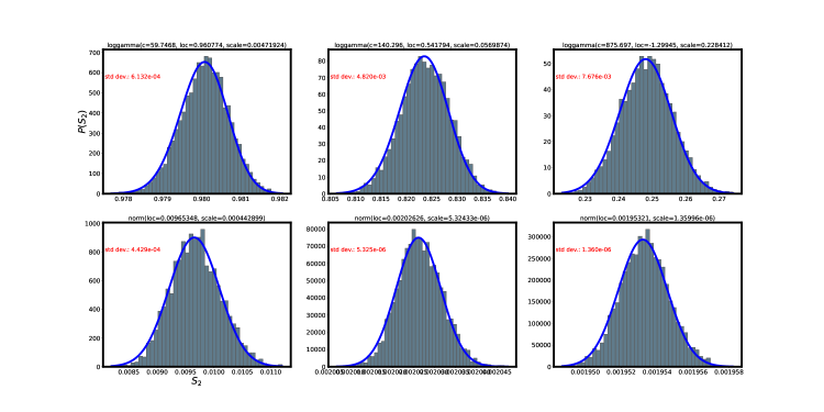
Figure 1: Distribution of purity ($S_{2}$) for the Brownian state ensemble (eq.(61)): The figure displays the distribution for different $Y$-values, ranging from almost separable limit, to intermediately entangled and highly entangled regimes respectively. The goodness of fit of the distribution has been tested minimizing the residual sum of squares (RSS). The ensemble size is taken to be $5000$. We note that that fluctuations in the intermediate regime is orders of magnitude larger than the two end points, viz., separability and maximum entanglement limits.

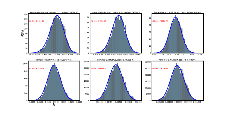
Figure 2: Distribution of purity for power-law state ensemble: The details here are same as in figure 1, except now the ensemble concerned is described by eq.(63).

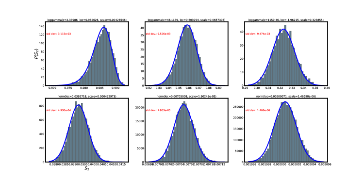
Figure 3: Distribution of purity for exponential state ensemble: The details here are same as in figures 1 and 2, except now the ensemble concerned is described by eq.(65).

Figures 1-3 depict the distributions of purity at six different $Y$-values for each of the BE, PE and EE respectively. As each figure indicates, the initial distribution is well-described by the Log-Gamma behavior ($f(x,c)=\frac{\exp(cx-e^{x})}{\Gamma(c)}$). A crossover occurs as $Y$ increases beyond its initial value $Y_{0}$ with large $Y$-limit converging to a Gaussian behavior ( $f(x)=\frac{\exp(-x^{2}/2)}{\sqrt{2\pi}}$). The crossover behavior for small $Y-Y_{0}$ is well-fitted by by the Log-Gamma behavior but the distribution parameters change (given in 1): this is consistent with our theoretical prediction for purity case discussed in previous section. Here the standard definitions of the distribution given above are subjected to additional shift (loc) and scale of the variable as $y=(x-loc)\,/\,scale$, such that, the standard PDF $f(x,c)$ is same as $f(y,c)\,/\,scale$. The details of the fitted parameters for each case are given in table 1.

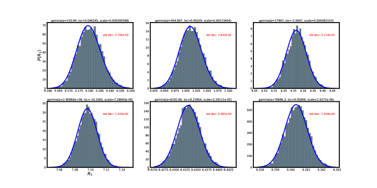
Figure 5: Distribution of von Neumann entropy for power-law state ensemble (eq.(63)): The details here are same as in figure 2, except now the measure considered here is von Neumann entropy $R_{1}$.

Figures 4-6 displays the distributions of von Neumann entropies (corresponding to each purity case depicted in Figures 1-3). The initial distribution is now well-fitted by the Gamma behavior ($f(x,a)=\frac{x^{a-1}\,e^{-x}}{\Gamma(a)}$). As predicted by our theory, the behavior during crossover as well as in large $Y$-limit in each case also remains Gamma distribution with fitted parameters for each case given in table 1.

As clear from each of the figures, the distribution of both entropies approach a narrow distribution for small $Y$ ($\to 0$) and large $Y\geq 1$, respectively. For intermediate $Y$ values ($Y\sim\frac{1}{N}$), however, the distributions have non-zero finite width. This indicates the following: as both entropies involve a sum over functions of the Schmidt eigenvalues, their local fluctuations are averaged out in separable and maximally entangled limit. For the partial entanglement region, corresponding to finite non-zero $Y$ (specifically, where average entropy changes from linear $Y$-dependence to a constant in $Y$), the eigenvalue fluctuations are too strong to be wiped out by summation, resulting in significant fluctuations of the entropies. It is also worth noting that the distribution for $Y\sim 1$ is almost same for all three cases; this suggests that the distributions are almost independent of ensemble details i.e., local constraints. Further, as for finite $N$ the fluctuations of $S_{2},R_{1}$ around their average can not be neglected, this has implications for ordering the states in increasing entanglement using purity or von Neumann entropy as the criteria. Furthermore, the distributions are dependent on subsystem sizes too (corresponding figures for unbalanced cases are not included here).

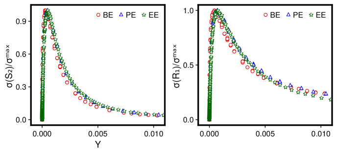
Figure 7: Parametric evolution of the standard deviation of purity and entanglement entropy: The figure displays the evolution of the standard deviation of the purity and von Neumann entropy for the three ensembles, defined in eq.(61), eq.(63) and eq.(65), as the complexity parameter varies from separability limit to maximum entanglement limit. The collapse for different ensembles signifies the universality of the parameter $Y$. Most interestingly, we see a spike when the system transitions from a separable to maximum entanglement regime. Such pattern is usually observed when the system goes under a quantum phase transition, e.g., thermalization to localization transition.

Figure 7 also displays the standard deviation of $S_{2}$ and $R_{1}$ changing with $Y$. As can be seen from the figure, although the standard deviation of entanglement measures in the separable and maximally entangled regimes is vanishing, as $N\to\infty$, in the intermediate regime the fluctuations are orders of magnitude larger. Observation of such trends in quantum fluctuation measures are believed to indicate a quantum phase transition PhysRevLett.90.227902 ; PhysRevA.66.032110 and the idea has already been used to study thermalization $\to$ many-body localization transition in disordered systems Luitz2015 . This indeed lends credence to the state matrix models used in our analysis: although mimicking underlying complexity of the state through Gaussian randomness, they turn out to be good enough to capture interesting many-body phenomena.

Table 1: Details of the fitted distributions in figures 1-6 : The parameters for the Log-Gamma distribution $f(x,c)=\frac{\exp(cx-e^{x})}{\Gamma(c)}$ is shown as L-Gamma(c, loc, scale). Similarly, for Gamma distribution $f(x,a)=\frac{x^{a-1}\,e^{-x}}{\Gamma(a)}$ as Gamma(a, loc, scale), and for Gaussian distribution $f(x)=\frac{\exp(-x^{2}/2)}{\sqrt{2\pi}}$ as Normal(loc, scale). The same details are also displayed in the figures 1-6. (For $R_{1}$, for $Y\gtrsim 10^{-2}$, the Normal distribution also turns out to be a good fit. The results presented here are such that it’s in best agreement with the theory.)

Measure	Ensemble	$Y\sim$
		$10^{-5}$	$~{}10^{-4}$	$~{}10^{-3}$	$~{}10^{-2}$	$~{}10^{-1}$	$~{}1$
$S_{2}$	BE	L-Gamma (59.75, 0.96, 0.0047)	L-Gamma (140.29, 0.54, 0.057)	L-Gamma (875.697, -1.29945, 0.228412)	Normal (0.00965, 0.00044)	Normal (0.00202, 5.32e-06)	Normal (0.0019, 1.36e-06)
	PE	L-Gamma (18.039, 0.96, 0.00436)	L-Gamma (56.205, 0.659, 0.04)	L-Gamma (1114.87, -1.574, 0.261)	Normal (0.01989, 0.000414)	Normal (0.004514, 1.44e-05)	Normal (0.0019, 1.454e-06)
	EE	L-Gamma (2.33986, 0.982626, 0.00428)	L-Gamma (48.1189, 0.603, 0.0657)	L-Gamma (1159.46, -1.96215, 0.32385)	Normal (0.03927, 0.000493)	Normal (0.00705, 1.902e-05)	Normal (0.002, 1.465e-06)
$R_{1}$	BE	Gamma (270.677, 0.093, 0.000299)	Gamma (568.46, 0.5085, 0.0014)	Gamma (5054.61, 0.5701, 0.001)	Gamma (646.788, 8.4982, 0.000592)	Gamma (754.305, 9.23393, 3.9387e-05)	Gamma (3543.41, 9.23622, 1.19628e-05)
	PE	Gamma (210.84, 0.096345, 0.00039)	Gamma (454.897, 0.45, 0.00123)	Gamma (17997, -2.5947, 0.000381)	Gamma (2.9096e+06, -14.106, 7.2869e-06)	Gamma (6292.66, 8.228, 3.261e-05)	Gamma (76696.3, 9.058, 2.6372e-06)
	EE	Gamma (16.6276, 0.021, 0.003072)	Gamma (370.069, 0.023, 0.0016)	Gamma (5459.14, -0.1287, 0.00052)	Gamma (48879.9, 3.05718, 4.62018e-05)	Gamma (1133.21, 7.4771, 7.299e-05)	Gamma (30515.2, 9.12597, 4.21196e-06)

VI Conclusion

In the end, we summarize with a brief discussion of our main idea, results, and open questions. We have theoretically analyzed the distribution of entanglement measures of a typical quantum state in a bi-partite basis. While previous theoretical studies have mostly considered ergodic states, leading to a standard Wishart ensemble representation of the reduced density matrix, our primary focus in this work has been on the non-ergodic states, specifically, the states with their components (in bi-partite basis) Gaussian distributed with arbitrary mean and variances, subjected to symmetry constraints, in addition. This in turn gives the reduced density matrix as a multi-parametric Wishart ensemble with fixed trace and permits an analysis of the entanglement with changing system conditions, i.e., complexity of the system. Our approach is based on the complexity parameter formulation of the joint probability distribution of the Schmidt eigenvalues which in turn leads to the evolution equations for the distributions of the Rényi and von Neumann entropies. As clearly indicated by the theoretical formulations for the probability densities for finite $Y$, reconfirmed by numerical analysis of the distributions and their standard deviation, a knowledge of the average entanglement measures is not sufficient for complex systems, their fluctuations are indeed significant, and any hierarchical arrangement of states based solely on the averages may lead to erroneous results.

The present study still leaves many open questions. For example, a typical many-body state of a quantum system may be subjected to additional constraints and need not be represented by a multiparametric Wishart ensemble with fixed trace only. It is then natural to query about the role of additional constraints on the growth of entanglement measure. The question is relevant in view of the recent studies indicating different time-dependent growth rates in constrained systems PhysRevResearch.2.033020 ; PhysRevLett.122.250602 . A generalization of the present results to bipartite mixed states as well as multipartite states is also very much desirable and will be presented in near future.

Another question is regarding the explicit role played by the system parameters in the entanglement evolution. The complexity parameter depends on the system parameters through distribution parameters. A knowledge of their exact relation, however, requires a prior knowledge of the quantum Hamiltonian, its matrix representation in the product basis as well as the nature and distribution parameters of the appropriate ensemble. The knowledge leads to the determination of the appropriate ensemble of its eigenstates. A complexity parameter formulation for the Hermitian operators, e.g., many-body Hamiltonians, and their eigenstates has already been derived. As the evolution equation of the JPDF of the components of an eigenfunction can in principle be derived from that of the ensemble density of the Hamiltonian, the evolution parameter of the former must be dependent on the latter. This work in currently in progress.

Appendix A Derivation of eqs. (15) and (43)

From the definition in eq.(11), we have for $k=2$, the JPDF $P_{2}$ of $S_{2}$ and $S_{1}$.

For $X(\lambda)$ as an arbitrary function of eigenvalues $\lambda_{1}\ldots\lambda_{N}$, the JPDF $P_{x}$ of $S_{1}$ and $X(\lambda)$ can be defined as

$$P_{x}(S_{1},X;Y)=\int\delta_{1}\;\delta_{x}\;P_{\lambda}(\lambda;Y)\;{\rm D}\lambda,$$ (67)

with $\delta_{x}\equiv\delta(X-X(\lambda)$ and $\delta_{1}$ defined below eq.(11) and $P_{\lambda}(\lambda)\to 0$ at the two integration limits $0\leq\lambda_{n}\leq\infty$ $\forall n=1\cdots N$. We note here that the constraint $\delta_{1}$ effectively reduces the limits to ${1\over N}\leq\lambda_{n}\leq 1$.

A differentiation of the above equation with respect to $Y$ and subsequently using eq.(67) gives

$$\frac{\partial P_{x}(S_{1},X;Y)}{\partial Y}=\int\delta_{1}\;\delta_{x}\;\frac{\partial P_{\lambda}}{\partial Y}\;{\rm D}\lambda=I_{1}+I_{2},$$ (68)

with $I_{1}$ as,

$$I_{1} = -C_{hs}\;\sum_{n=1}^{N}\int_{0}^{\infty}\;\delta_{1}\;\delta_{x}\;\frac{\partial}{\partial\lambda_{n}}\left(\sum_{m=1}^{N}\frac{\beta\lambda_{n}}{\lambda_{n}-\lambda_{m}}+{\beta\nu}-{2\gamma}\lambda_{n}\right)\;P_{\lambda}\;{\rm D}\lambda,$$ (69)

and,

$$I_{2} = C_{hs}\;\sum_{n=1}^{N}\int\;\delta_{1}\;\delta_{x}\;\frac{\partial^{2}(\lambda_{n}\;P_{\lambda})}{\partial\lambda_{n}^{2}}\;{\rm D}\lambda.$$ (70)

Integration by parts, and, subsequently using the relation $P_{\lambda}(\lambda)\to 0$ at the integration limits, now gives

$$I_{1} = C_{hs}\;\sum_{n=1}^{N}\int_{0}^{\infty}\;\left[\frac{\partial\delta_{1}}{\partial\lambda_{n}}\;\delta_{x}+\delta_{1}\;\frac{\partial\delta_{x}}{\partial\lambda_{n}}\right]\;\left(\sum_{m=1}^{N}\frac{\beta\lambda_{n}}{\lambda_{n}-\lambda_{m}}+{\beta\nu}-{2\gamma}\lambda_{n}\right)P_{\lambda}\;{\rm D}\lambda.$$ (71)

Again using $\frac{\partial\delta_{a}}{\partial\lambda_{n}}=-\frac{\partial\delta_{a}}{\partial a}\frac{\partial a(\lambda)}{\partial\lambda_{n}}$ with $a=S_{1}$ or $X$, $I_{1}$ can be rewritten as

$$I_{1} = \frac{\partial}{\partial S_{1}}\left(2\;\gamma\;S_{1}-{1\over 2}\beta N(N+2\nu-1)\right)\;P_{x}+I_{0},$$ (72)

where,

$$I_{0}=-C_{hs}\;\frac{\partial}{\partial X}\ \int\delta_{1}\;\delta_{x}\;\left[\sum_{n=1}^{N}\frac{\partial X}{\partial\lambda_{n}}\;\left(\sum_{m=1}^{N}\frac{\beta\lambda_{n}}{\lambda_{n}-\lambda_{m}}+\left({\beta\nu}-{2\gamma}\lambda_{n}\right)\right)\right]\;P_{\lambda}\;{\rm D}\lambda.$$ (73)

Similarly, a repeated partial differentiation gives

$$I_{2} = C_{hs}\;\sum_{n=1}^{N}\int\;\left[\;\delta_{1}\;\frac{\partial^{2}\delta_{x}}{\partial\lambda_{n}^{2}}+2\frac{\partial\delta_{1}}{\partial\lambda_{n}}\;\frac{\partial\delta_{x}}{\partial\lambda_{n}}+\frac{\partial^{2}\delta_{1}}{\partial\lambda_{n}^{2}}\;\delta_{x}\right]\;\lambda_{n}\;P_{\lambda}\;{\rm D}\lambda.$$ (74)

Again using $\frac{\partial^{2}\delta_{x}}{\partial\lambda_{n}^{2}}=\frac{\partial^{2}\delta_{x}}{\partial x^{2}}\;\left(\frac{\partial X(\lambda)}{\partial\lambda_{n}}\right)^{2}-\frac{\partial\delta_{x}}{\partial X}\frac{\partial^{2}X(\lambda)}{\partial\lambda_{n}^{2}}$ and $\frac{\partial^{2}\delta_{1}}{\partial\lambda_{n}^{2}}=\frac{\partial^{2}\delta_{1}}{\partial S_{1}^{2}}$, $I_{2}$ can be rewritten as

$$I_{2} = C_{hs}\;\sum_{n=1}^{N}\int\;\left[\;\delta_{1}\;\left(\frac{\partial^{2}\delta_{x}}{\partial X^{2}}\;\left(\frac{\partial X}{\partial\lambda_{n}}\right)^{2}-\frac{\partial\delta_{x}}{\partial X}\frac{\partial^{2}X}{\partial\lambda_{n}^{2}}\right)+2\frac{\partial\delta_{1}}{\partial S_{1}}\;\frac{\partial\delta_{x}}{\partial X}\frac{\partial X}{\partial\lambda_{n}}+\frac{\partial^{2}\delta_{1}}{\partial S_{1}^{2}}\;\delta_{x}\right]\;\lambda_{n}\;P_{\lambda}\;{\rm D}\lambda.$$

Based on the details of function $X(\lambda)$, the integrals $I_{1}$ and $I_{2}$ can further be reduced. Here we give the results for $S_{2}$ and $R_{1}$.

Case $X=S_{2}$: Proceeding similarly for $X(\lambda)=\sum_{n}\lambda_{n}^{2}$, we have, from eq. (72) and eq. (73),

$$I_{1} = \frac{\partial}{\partial S_{1}}(2\;\gamma\;S_{1}-{1\over 2}\beta N(N+2\nu-1))\;P_{2}+I_{0}.$$ (76)

and

$$I_{0} = -2C_{hs}\;\frac{\partial}{\partial S_{2}}\int\delta_{1}\;\delta_{2}\;\left(\sum_{m,n=1}^{N}\frac{\beta\lambda_{n}^{2}}{\lambda_{n}-\lambda_{m}}+{\beta\nu}\sum_{n=1}^{N}\;\lambda_{n}-{2\gamma}\sum_{n=1}^{N}\;\lambda_{n}^{2}\right)P_{\lambda}\;{\rm D}\lambda.$$ (77)

Using the equality $2\;\sum_{m,n=1}^{N}\frac{\lambda_{n}^{2}}{\lambda_{n}-\lambda_{m}}=\sum_{m,n=1}^{N}\frac{\lambda_{n}^{2}-\lambda_{m}^{2}}{\lambda_{n}-\lambda_{m}}=2(N-1)\sum_{n}\lambda_{n}$, $I_{0}$ can be rewritten as

$$I_{0} = -C_{hs}\;\frac{\partial}{\partial S_{2}}\int\delta_{1}\;\delta_{2}\;\left(2(N-1+\nu)\beta\;S_{1}-{4\gamma}\;S_{2}\right)P_{\lambda}\;{\rm D}\lambda$$ (78)

$$= -\frac{\partial}{\partial S_{2}}\left(2(N-1+\nu)\beta\;S_{1}-{4\gamma}\;S_{2}\right)P_{2}.$$ (79)

Proceeding similarly, from eq. (LABEL:i2xc) we have

$$I_{2} = 4\frac{\partial^{2}}{\partial S_{2}^{2}}I_{3}-2\frac{\partial}{\partial S_{2}}(S_{1}P_{2})+4\frac{\partial^{2}}{\partial S_{1}\partial S_{2}}(S_{2}P_{2})+\frac{\partial^{2}}{\partial S_{1}}(S_{1}P_{2}).$$ (80)

Substitution of eq.(76) and eq.(80) in eq.(68) for $X=S_{2}$ now leads to

$$\frac{\partial P_{2}}{\partial Y}=4\frac{\partial^{2}(S_{2}\;P_{2})}{\partial S_{2}\partial S_{1}}+4\frac{\partial^{2}I_{3}}{\partial S_{2}^{2}}+\frac{\partial^{2}(S_{1}\;P_{2})}{\partial S_{1}^{2}}+2\frac{\partial(Q_{2}\;P_{2})}{\partial S_{2}}+\frac{\partial(Q_{1}\;P_{2})}{\partial S_{1}},$$ (81)

with $Q_{2}\equiv(2\gamma S_{2}-\beta(N+\nu-1)S_{1}-S_{1})$, $Q_{1}=2\gamma S_{1}-{\beta\over 2}N(N+2\nu-1)$ and

$$I_{3}=\int\prod_{k=1}^{2}\;\delta_{S_{k}}\;\left(\sum_{n}\lambda_{n}^{3}\right)\;P_{\lambda}\;{\rm D}\lambda=\int\;S_{3}\;P_{3}(S_{1},S_{2},S_{3})\;{\rm d}S_{3}.$$ (82)

Case $X=R_{1}$: Following from above, we have for $X(\lambda)=-\sum_{n}\lambda_{n}\log\lambda_{n}$,

$$I_{1} = \frac{\partial}{\partial S_{1}}(2\;\gamma\;S_{1}-{1\over 2}\beta N(N+2\nu-1))\;P_{v}(S_{1},R_{1},Y)+I_{0},$$ (83)

and

$$I_{0} = C_{hs}\frac{\partial}{\partial R_{1}}\;\int\;\delta_{1}\;\delta_{v}\left[\sum_{m,n=1}^{N}\frac{\beta\lambda_{n}\left(1+\log\lambda_{n}\right)}{\lambda_{n}-\lambda_{m}}+{\beta\nu}\sum_{n}\left(1+\log\lambda_{n}\right)-{2\gamma}\sum_{n}\lambda_{n}\left(1+\log\lambda_{n}\right)\right]\;P_{\lambda}{\rm D}\lambda.$$

Further, using the relation $\sum_{n\neq m}\frac{\lambda_{n}\log\lambda_{n}}{\lambda_{n}-\lambda_{m}}\approx\frac{N(N-1)}{2}-\frac{(N-1)}{2}R_{0}$ where $R_{0}(\lambda)\equiv-\sum_{n}\log\lambda_{n}$ (derived in appendix J of Shekhar_2023 ), eq.(LABEL:i0r1a) can be rewritten as

$$I_{0}=\frac{\partial}{\partial R_{1}}\left[\left(\beta N(N+\nu-1)+2\gamma(R_{1}-S_{1})-\beta\frac{N_{\nu}}{2}R_{0}\right)P_{v}\right].$$ (85)

Substitution of eq.(83) and eq.(85) in eq.(72), we have for $X=R_{1}$,

$$I_{1} = \frac{\partial}{\partial S_{1}}\left[\left(2\;\gamma\;S_{1}-{1\over 2}\beta N(N+2\nu-1)\right)\;P_{v}\right]$$ (86)

$$+ \frac{\partial}{\partial R_{1}}\left[\left(\beta N(N+\nu-1)+2\gamma(R_{1}-S_{1})-\beta\frac{N_{\nu}}{2}R_{0}\right)P_{v}\right].$$

Substituting $X=-\sum_{n}\lambda_{n}\log\lambda_{n}$ in eq.(LABEL:i2xc),

$I_{2}$ can be written as

$$I_{2} = \frac{\partial^{2}}{\partial R_{1}^{2}}\left((S_{1}-2R_{1})P_{v}+J_{1}\right)-2\frac{\partial^{2}}{\partial S_{1}\partial R_{1}}\left((S_{1}-R_{1})P_{v}\right)$$ (87)

$$+ N\frac{\partial}{\partial R_{1}}P_{v}+\frac{\partial^{2}}{\partial S_{1}^{2}}(S_{1}P_{v}),$$

with

$$J_{k} = \int\delta_{R_{1}}\;\delta_{S_{1}}\;\left[\sum_{n}(\lambda_{n})^{k}(\log\lambda_{n})^{k+1}\right]\;P_{\lambda}\;{\rm D}\lambda,$$ (88)

where $\delta_{R_{1}}\equiv\delta(R_{1}+\sum_{n}\lambda_{n}\;{\rm log}\lambda_{n})$ and $\delta_{S_{1}}\equiv\delta(S_{1}-\sum_{n}\lambda_{n})$.
$\Rightarrow$

$$\frac{\partial P_{v}}{\partial Y} = 2\frac{\partial^{2}}{\partial R_{1}\partial S_{1}}\left[(R_{1}-S_{1})\;P_{v}\right]+\frac{\partial^{2}}{\partial R_{1}^{2}}\left[(S_{1}-2R_{1})P_{v}+J_{1}\right]+\frac{\partial^{2}}{\partial S_{1}^{2}}(S_{1}\;P_{v})$$ (89)

$$+ \frac{\partial}{\partial R_{1}}\left[\left(\beta N(N+\nu-1)+2\gamma(R_{1}-S_{1})-\beta\frac{N_{\nu}}{2}\langle R_{0}\rangle+N\right)P_{v}\right]$$

$$+ \frac{\partial}{\partial S_{1}}\left[\left(2\;\gamma\;S_{1}-{1\over 2}\beta NN_{\nu}\right)\;P_{v}\right].$$

To express the above integral in terms of $P_{v}$, we can approximate them as follows. We rewrite $J_{k}$ as

$$J_{k}=\int T_{k}\;P(R_{1},S_{1},T_{k})\;{\rm d}T_{k},$$ (90)

with

$$P(R_{1},S_{1},T_{k})=\int\delta_{R_{1}}\;\delta_{S_{1}}\delta_{T_{k}}\;P_{\lambda}\;{\rm D}\lambda,$$ (91)

and $T_{k}=\sum_{n}(\lambda_{n})^{k}(\log\lambda_{n})^{k+1}$. Further, noting that $T_{k}$ varies more rapidly than $R_{1}$ and $S_{1}$ for large $N$, we can approximate $P(S_{1},R_{1},T_{k})\approx P_{T}(T_{k})\;P_{v}(R_{1},S_{1})$. The latter on substitution in eq.(90) gives

$$J_{k}\approx\langle T_{k}\rangle\;P_{v}(R_{1},S_{1}).$$ (92)

Appendix B Solution of eq. (17)

For large $Y$, $\langle S_{3}\rangle$ approaches a constant: $\langle S_{3}\rangle\sim{1\over N^{2}}$. Again using separation of variables and for arbitrary initial condition at $Y=Y_{0}$, the solution can be given as

$$\Psi(x;Y)={\rm e}^{-E\;(Y-Y_{0})}\;V(x;E),$$ (93)

where $V(x,E)$ is the solution of the differential equations

$$\frac{{\rm d}^{2}V}{{\rm d}x^{2}}+2x\;\frac{{\rm d}V}{{\rm d}x}+{d\over 2\omega}\;V=0,$$ (94)

with $\eta\approx 4\,\omega+2\gamma\approx 4\omega$, $d=d_{0}+E$ with $E$ as an arbitrary semi-positive constant and $d_{0}=(\gamma-\beta NN_{\nu})\,{\omega\over 2}+\omega^{2}+4\gamma+1$. In large $N$ limit, $d_{0}$ can further be approximated as $d_{0}\approx{\omega\over 2}\,(2\omega-\beta NN_{\nu})>0$ (assuming $\omega\gg NN_{\nu},\gamma$). A solution of eq.(94) can now be given as

$$V(x;E)={\rm e}^{-{x^{2}}}\;\left(c_{1}(E)\;H_{2\mu}\left(x\right)+c_{2}(E)\;F_{1}\left(-{\mu},{1\over 2},x^{2}\right)\right),$$ (95)

with $\mu=\frac{d-4w}{8w}\approx{d\over 8\omega}$. The constants of integration $c_{1},c_{2}$ are determined from the boundary conditions. Here $H_{\mu}(x)$ is the Hermite’s function and $F_{1}(-\mu,\zeta;z)\equiv_{1}F_{1}(-\mu,\zeta;z)$ is the confluent hypergeometric function defined as $F_{1}(-\mu,\zeta;z)=\sum_{k=0}^{\infty}{(-\mu)_{k}\,z^{k}\over k!\,\zeta_{k}}$ with symbol $a_{k}\equiv\prod_{n=0}^{k-1}(a+n)$.

Further, noting that

$$H_{2\mu}\left(x\right)={2^{2\mu}\sqrt{\pi}\over\Gamma{({1-2\mu\over 2})}}\;F_{1}\left(-{\mu},{1\over 2},x^{2}\right)-{2^{2\mu+1}\sqrt{\pi}\over\Gamma{(-{\mu})}}\;x\;F_{1}\left({1-2\mu\over 2},{3\over 2},x^{2}\right),$$

eq.(95) can be rewritten as

$$V(S_{2};E)={\rm e}^{-{x^{2}}}\;\left(c_{3}(E)\,F_{1}\left(-{\mu},{1\over 2},x^{2}\right)+c_{4}(E)\,x\,F_{1}\left({1-2\mu\over 2},{3\over 2},x^{2}\right)\right),$$ (96)

with $c_{3}(E)={2^{2\mu}\sqrt{\pi}\over\Gamma{({1-2\mu\over 2})}}c_{1}+c_{2}$ and $c_{4}(E)=-{2^{2\mu+1}\sqrt{\pi}\;c_{1}\over\Gamma{(-{\mu})}}$.

As $E$ is an arbitrary constant and $g(S_{1})$ is an arbitrary function of $S_{1}$, it is easier to write, without loss of generality, $E=|d_{0}|\,m=8\omega\mu_{0}m$ with $m$ as a semi-positive integer, satisfying the condition $E\geq 0$. This gives $d=|d_{0}|(m+s_{0}))$ and thereby $\mu\equiv\mu_{m}={|d_{0}|\over 8\,\omega}(m+s_{0})$ with $s_{0}=1,0,-1$ if $d_{0}>0,0,<0$ respectively. The general solution for $\Psi(x,Y)$ can now be written as

$$\Psi(x;Y)={\rm e}^{-{x^{2}}}\sum_{m=0}^{\infty}\;{\rm e}^{-8\omega\mu_{0}\,m\;(Y-Y_{0})}\,\left(c_{3m}\,F_{1}\left(-{\mu_{m}},{1\over 2},x^{2}\right)+c_{4m}\,x\,F_{1}\left({1-2\mu_{m}\over 2},{3\over 2},x^{2}\right)\right).$$

(97)

Further, following the relation

$$x^{2}\,F_{1}\left({1-\mu_{m}\over 2},{3\over 2},x^{2}\right)={1\over 2}\;\left[F_{1}\left({1-\mu_{m}\over 2},{1\over 2},x^{2}\right)-F_{1}\left(-{1+\mu_{m}\over 2},{1\over 2},x^{2}\right)\right],$$

we have, for large $\mu_{m}$, $x^{2}\,F_{1}\left({1-\mu_{m}\over 2},{3\over 2},x^{2}\right)\approx 0$. For $x>0$, the contribution from the second term in eq.(97) can then be neglected, leading to following form

$$\Psi(x;Y)\approx{\rm e}^{-{x^{2}}}\,\sum_{m=0}^{\infty}\;{\rm e}^{-8\,\omega\,\mu_{0}\,m\;(Y-Y_{0})}\,F_{1}\left(-{\mu_{m}},{1\over 2},x^{2}\right)\,C_{m},$$ (98)

with $C_{m}$ as constants to be determined from initial conditions. As ${\mu_{0}}={1\over 8}(2\omega-\beta NN_{\nu})$ for our case, hereafter we set $\omega\sim\beta N^{2}/4q$ with $q\sim o(1)$ for clarity of analysis; (we note $q<1/2$ to keep $d_{0}>0$).

To proceed further, we use following relation: for $a\to\infty$, $|ph(a)|\leq\pi-\delta$ and $b$, $z$ fixed

$${\mathbf{F}}\left(-a,b,z\right)\sim\left(z/a\right)^{(1-b)\over 2}\frac{e^{z/2}\Gamma\left(1+a\right)}{\Gamma\left(a+b\right)}\*\left(J_{b-1}\left(2\sqrt{az}\right)\sum_{s=0}^{\infty}\frac{p_{s}(z)}{(-a)^{s}}-\sqrt{z/a}\;J_{b}\left(2\sqrt{az}\right)\sum_{s=0}^{\infty}\frac{q_{s}(z)}{(-a)^{s}}\right),$$

(99)

with $p_{k}(z)=\sum_{s=0}^{k}\genfrac{(}{)}{0.0pt}{}{k}{s}{\left(1-b\right)_{k-s}}z^{s}c_{k+s}(z),$ $q_{k}(z)=\sum_{s=0}^{k}\genfrac{(}{)}{0.0pt}{}{k}{s}{\left(2-b\right)_{k-s}}z^{s}c_{k+s+1}(z),$ where $(k+1)c_{k+1}(z)+\sum_{s=0}^{k}\left(\frac{bB_{s+1}}{(s+1)!}+\frac{z(s+1)B_{s+2}}{(s+2)!}\right)c_{k-s}(z)=0.$ Substitution of eq.(99) in eq(98) now leads to eq.(27) in section III.1.

To elucidate determination of $C_{m}$ from initial probability density, we consider following distribution of $S_{2}$ in the separability limit (motivated by our numerical analysis discussed later),

$$\Psi(x;Y_{0})=a_{0}\;{\rm exp}\left[-\omega_{0}(x-b_{0})-{\rm exp}\left(\omega_{1}(x-b_{0})\right)\right],$$ (100)

with $a_{0},\,\omega_{0},\,\omega_{1}$ as known constants (known as (Log Gamma) distribution). Substitution of the above in eq.(30) for $Y=Y_{0}$ and using $x=S_{2}\sqrt{\omega_{2}}$ (eq.(23)) with $\omega_{2}={\omega\over 2\langle S_{3}\rangle}$) now leads to

$$C_{m} = \frac{a_{0}\,a_{1}\,\omega_{2}}{\pi}\int_{1/N}^{1}{\rm d}S_{2}\;{\rm exp}\left[{{\omega_{2}S_{2}^{2}/2}-\omega_{2}S_{2}-a_{2}\,{\rm e}^{\omega_{1}\sqrt{\omega_{2}}\,S_{2}}}\right]\,\cos\left(S_{2}\,\sqrt{4\mu_{m}\omega_{2}}\right)$$ (101)

with $a_{1}={\rm e}^{\omega_{0}b_{0}}$ and $a_{2}={\rm e}^{-{\rm e}^{-\omega_{0}b_{0}}}$. As both $\mu_{m}$ as well as $\omega_{2}$ are large for entire range of integration, a rapid oscillation of $\cos$ term results in a significant contribution, coming for small $m$ values only, from lowest range of integration.

Although for any finite non-zero $Y-Y_{0}$, the factor ${\mathcal{Y}}_{m}\equiv e^{-8\omega\mu_{0}\;m(Y-Y_{0})}$ in eq.(27) becomes vanishingly small for $m>0$, but as $C_{0},C_{1}\sim\omega_{2}a_{0}a_{1}$, their large value can compensate the small values of coefficients ${\mathcal{Y}}_{0},{\mathcal{Y}}_{1}$ and can thereby can lead to an intermediate state for $f_{2}(S_{2};Y)$, different from those at $Y=Y_{0}$ and $Y\to\infty$.

Appendix C Solution of eq.(44)

Using separation of variables again, a solution of eq.(44) for arbitrary initial condition at $Y=Y_{0}$ can be written as

$$f_{v,\omega}(R_{1};Y)={\rm e}^{-E\;(Y-Y_{0})}\;V(R_{1};E),$$ (102)

with $V(R_{1},E)$ as the solution of the differential equation

$$(t-2R_{1})\;\frac{{\rm d}^{2}V}{{\rm d}R_{1}^{2}}+(aR_{1}+b)\;\frac{{\rm d}V}{{\rm d}R_{1}}+d\;V=0,$$ (103)

with $a=2\gamma+2\,\omega\approx 2\omega$ (assuming $\gamma$ finite), $b=\beta\,(N_{\nu}-\nu)\,N-{\beta\over 2}N_{\nu}\,\langle R_{0}\rangle+N+2\,\omega-2\gamma-4$ where $R_{0}=-\sum\log\lambda_{n}$, $d=E+d_{0}$ and $d_{0}={\beta\over 2}\,\omega\,N\,N_{\nu}+\omega^{2}+(2-2\gamma)\;\omega-4$, $t=1+\langle T_{1}\rangle\sim 1+\langle R_{1}\rangle^{2}$, $N_{\nu}=N+2\nu-1$ and $E$ as an arbitrary positive constant determined by the initial conditions on $V$. A solution of eq.(103) can now be given as

$$V(R_{1};E)=\left({8x\over a}\right)^{\alpha}\;\left(c_{1}\;U\left[\alpha+{d\over a},\alpha+1,x\right]+c_{2}\;L\left[-\left(\alpha+{d\over a}\right),\alpha,x\right]\right),$$

(104)

with $x\equiv-a(t-2R_{1})/4$ (used for compact writing), $c_{1},c_{2}$ as unknown constants of integration, $\alpha={1\over 4}(at+2b+4)$. Here $U$ is a confluent hypergeometric function of first kind, defined as

$$U(a,b,x)={\Gamma(b-1)\over\Gamma(a)}\,x^{1-b}\,F_{1}(a-b+1,2-b,x)+{\Gamma(1-b)\over\Gamma(a-b+1)}\,F_{1}(a,b,x),$$

with $F_{1}(a,b,x)=_{1}{\tilde{F}}_{1}$ as the hypergeometric function defined as ${}_{1}{F}_{1}(a,b,x)=\sum_{k=0}^{\infty}{(a)_{k}\,x^{k}\over(b)_{k}\,k!}$. The above definition is valid for $b$ not an integer. Here, for $b$ as an integer, it should be replaced by $b_{1}$ where $b$ is integer limit of $b_{1}$. Further $L_{a}^{b}(x)\equiv L(a,b;x)$ is the associated Laguerre polynomial, defined as

$$L(a,b,x)={\Gamma(a+b+1)\over\Gamma(a+1)\,\Gamma(b+1)}\,_{1}{F}_{1}(-a,b+1,x).$$

Using the above relations, eq.(104) can be rewritten as

$$V(R_{1};E)=\left({8x\over a}\right)^{\alpha}\;\left(C_{1}\;F_{1}\left[\alpha+{d\over a},\alpha+1,x\right]+C_{2}\,x^{-\alpha}\,F_{1}\left[{d\over a},1-\alpha,x\right]\right).$$ (105)

Here again, with both $E$ and $\omega$ arbitrary in eq.(102), we can write, without loss of generality, $E=m\,|d_{0}|$ where $m$ is an arbitrary non-negative integer.

In large $N$ and $\omega$ limits, we have $a\approx 2\omega$, $b\approx\beta NN_{\nu}+2\omega-{\beta\over 2}N_{\nu}\langle R_{0}\rangle$ with $\langle R_{0}\rangle\sim N\log N$ Shekhar_2023 , $d_{0}\approx\omega\,\left({\beta\over 2}NN_{\nu}+\omega\right)>0$, this results in

The general solution can now be written as

$$f_{v,\omega}(R_{1};Y)=\sum_{m=0}^{\infty}{\rm e}^{-\,m\,|d_{0}|\;(Y-Y_{0})}\;V_{m}(R_{1};E),$$ (106)

with,

$$V_{m}(R_{1};E) = \left({4x\over\omega}\right)^{\alpha}\;\left(C_{1m}\;F_{1}\left(\alpha+{d_{m}\over 2\omega},\alpha+1,x\right)+C_{2m}\;x^{-\alpha}\,F_{1}\left({d_{m}\over 2\omega},1-\alpha,x\right)\right),$$

with $x\equiv-{\omega\over 2}(t-2R_{1})\sim-{\omega\over 2}(1+\langle R_{1}\rangle^{2}-2R_{1})$ and $d_{m}=d_{0}(1+m)\approx(m+1)\,\omega\,\left({\beta\over 2}NN_{\nu}+\omega\right)$ and $\alpha\approx{1\over 2}(\omega\,t+b)$.

Further, as the contribution from the second term in eq.(LABEL:vm1) is negligible as compared to first term, and we can approximate $V_{m}(R_{1};E)=\left({4x\over\omega}\right)^{\alpha}\;C_{1m}\;F_{1}\left(\alpha+{d_{m},\over 2\omega},\alpha+1,x\right)$

$$f_{v,\omega}(R_{1};Y)=\left({4x\over\omega}\right)^{\alpha}\;{\rm e}^{x}\;\sum_{m=0}^{\infty}C_{m}\;{\rm e}^{-\,{m\,\mid d_{0}\mid\;(Y-Y_{0})}}\;\;F_{1}\left(1-{d_{m},\over 2\omega},\alpha+1,-x\right).$$ (108)

Appendix D Calculation of variance of purity from eq.(17)

Eq.(17) describes the $Y$-evolution of the distribution $f_{2}$ of the purity $S_{2}$. This can further be used to derive the $Y$-evolution of the variance of $S_{2}$. Using the definition of variance $\langle\Delta S_{2}^{2}\rangle\equiv\langle S_{2}^{2}\rangle-\langle S_{2}\rangle^{2}$ and the $n^{th}$ order moment as $\langle S^{n}_{2}(Y)\rangle=\frac{\int S^{n}_{2}\,f_{2}(S_{2},Y)\,dS_{2}}{\int f_{2}\,dS_{2}}$, we have

$$\frac{\partial\langle\Delta S_{2}^{2}\rangle}{\partial Y} = \frac{\partial\langle S_{2}^{2}\rangle}{\partial Y}-2\langle S_{2}\rangle\frac{\partial\langle S_{2}\rangle}{\partial Y},$$ (109)

where,

$$\frac{\partial\langle S^{n}_{2}\rangle}{\partial Y} = \frac{\int S^{n}_{2}\,\frac{\partial f_{2}}{\partial Y}\,dS_{2}}{\int f_{2}dS_{2}}-\langle S_{2}\rangle\frac{\int\frac{\partial f_{2}}{\partial Y}\,dS_{2}}{\int f_{2}dS_{2}}.$$ (110)

Substitution of the eq.(17) in the above equation, with

$a=4\langle S_{3}\rangle,\,\eta\approx 4\omega,\,b=-(N_{a}+N_{b}-1)\beta$; repeated partial integration of the terms in right side of the above equation gives

$$\frac{\partial\langle S_{2}\rangle}{\partial Y} = -b-\eta\,\langle S_{2}\rangle$$ (111)

$$\frac{\partial\langle S_{2}^{2}\rangle}{\partial Y} = 2a-2\eta\,\langle S_{2}^{2}\rangle-2\,b\,\langle S_{2}\rangle$$ (112)

Substitution of eq. (111) and eq.(112) in eq.(109) then leads to

$$\frac{\partial\langle\Delta S_{2}^{2}\rangle}{\partial Y} = 2\,a-2\eta\langle\Delta S_{2}^{2}\rangle.$$ (113)

The above equation can now be solved to give

$$\langle\Delta S_{2}^{2}\rangle = \frac{a}{\eta}-A\,e^{-2\eta Y},$$ (114)

where the constant of integration $A$ is determined by the initial condition which is system dependent. Nonetheless, since, $\omega\sim N^{2}$, and $\langle S_{3}\rangle\sim\frac{1}{N^{2}},$we infer that in the stationary limit, $Y\to\infty$, $\langle\Delta S_{2}^{2}\rangle\sim\frac{1}{N^{4}}$, verified numerically in section V.

Appendix E Calculation of variance of von Neumann entropy from eq.(LABEL:pv1)

With variance defined as $\langle\Delta R_{1}^{2}\rangle\equiv\langle R_{1}^{2}\rangle-\langle R_{1}\rangle^{2}$ with $\langle R_{1}^{n}(Y)\rangle=\frac{\int R_{1}^{n}\,f_{v}(R_{1},Y)\,dR_{1}}{\int f_{v}\,dR_{1}}$, here again we have

$$\frac{\partial\langle\Delta R_{1}^{2}\rangle}{\partial Y} = \frac{\partial\langle R_{1}^{2}\rangle}{\partial Y}-2\langle R_{1}\rangle\frac{\partial\langle R_{1}\rangle}{\partial Y},$$ (115)

where,

$$\frac{\partial\langle R^{n}_{1}\rangle}{\partial Y} = \frac{\int R^{n}_{1}\,\frac{\partial f_{v}}{\partial Y}\,dR_{1}}{\int f_{v}dR_{1}}-\langle R_{1}\rangle\frac{\int\frac{\partial f_{v}}{\partial Y}\,dR_{1}}{\int f_{v}dR_{1}}.$$ (116)

Substituting eq. (44) into eq. (116), with $t\approx 1-R_{1}^{2}$, $a\approx 2w,\,b\approx\beta N(N+\nu-1)-\beta\frac{N_{\nu}}{2}\langle R_{0}\rangle+N+2\omega$, and repeating the steps in the preceding section we get,

$$\frac{\partial\langle R_{1}\rangle}{\partial Y} = (4-a)\langle R_{1}\rangle-(4+b)$$ (117)

$$\frac{\partial\langle R_{1}^{2}\rangle}{\partial Y} = (6-2a)\langle R_{1}^{2}\rangle-2(4+b)\langle R_{1}\rangle+2.$$ (118)

Substitution of the above equations in eq.(115), and, as $b$ and $a$ are large, we can approximate

$$\frac{\partial\langle\Delta R_{1}^{2}\rangle}{\partial Y}=-2a\langle\Delta R_{1}^{2}\rangle+2,$$ (119)

or,

$$\langle\Delta R_{1}^{2}\rangle=\frac{1}{a}-Be^{-2aY}.$$ (120)

That is, in the stationary limit $\langle\Delta R_{1}^{2}\rangle\sim\frac{1}{N^{2}}$, which is much larger that the fluctuations in purity, which we verify numerically.

Appendix F Figures

Figure 4: Distribution of von Neumann entropy for Brownian state ensemble (eq.(61)): The details here are same as in figure 1, except now the entanglement measure considered here is the von Neumann entropy $R_{1}$.

Figure 6: Distribution of von Neumann entropy for exponential state ensemble (eq.(65)): The details here are same as in figure 3, except now the measure considered here is von Neumann entropy $R_{1}$.