FedShift: Tackling Dual Heterogeneity Problem of Federated Learning via Weight Shift Aggregation

Abstract

Federated Learning (FL) offers a compelling method for training machine learning models with a focus on preserving data privacy. The presence of system heterogeneity and statistical heterogeneity, recognized challenges in FL, arises from the diversity of client hardware, network, and dataset distribution. This diversity can critically affect the training pace and the performance of models. While many studies address either system or statistical heterogeneity by introducing communication-efficient or stable convergence algorithms, addressing these challenges in isolation often leads to compromises due to unaddressed heterogeneity. In response, this paper introduces FedShift, a novel algorithm designed to enhance both the training speed and the models’ accuracy in a dual heterogeneity scenario. Our solution can improve client engagement through quantization and mitigate the adverse effects on performance typically associated with quantization by employing a shifting technique. This technique has proven to enhance accuracy by an average of 3.9% in diverse heterogeneity environments.

1 Introduction

As the demand for data privacy escalates, the necessity for safeguarding measures in machine learning intensifies. In response, technologies such as Federated Learning (FL) have emerged, offering a means to train neural network models while maintaining the privacy of data (McMahan et al., 2017; Konečnỳ et al., 2016; Shokri & Shmatikov, 2015).

In an FL environment, where model weights are exchanged between a central server and clients, the diversity of client environments can create systems heterogeneity and statistical heterogeneity. Systems heterogeneity, encompassing hardware and network performance, can lead to varying training and transmission times among clients, causing delays in model delivery to the central server. This delay, often due to slower clients, can extend the overall training time (Bonawitz et al., 2019). Statistical heterogeneity, stemming from non-independent and identically distributed (non-IID) data across clients, affects convergence rates and may degrade the global model’s performance (Zhao et al., 2018).

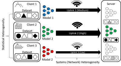
Figure 1: The coexistence of systems heterogeneity (network speed) and statistical heterogeneity (data distribution)

When systems and statistical heterogeneity coexist, as illustrated in Figure 1, clients in different geographical locations face varied network environments and possess distinct datasets. Traditional FL algorithms like FedAvg do not address this dual heterogeneity scenario where balancing model performance and training time is challenging. Involving all clients in the training process causes the slowest participant to determine the length of each training round, whereas excluding slower clients by imposing time-outs results in training sessions that proceed with partial datasets. Previous studies have typically focused either on improving communication efficiency by tackling system heterogeneity (Xie et al., 2019; Sun et al., 2019; Hamer et al., 2020) or on enhancing convergence stability by addressing statistical heterogeneity (Luo et al., 2021; Yuan et al., 2021).

We identify three approaches for enhancing client engagement and mitigating the impact of slower clients in FL. First is the adaptive aggregation technique, exemplified by FedProx (Li et al., 2020) and FedNova (Wang et al., 2020), which can minimize delays by varying the number of local epochs for each client based on their hardware and model performance. Another approach is to overcome the synchronization bottleneck by adopting asynchronous aggregation of global models, deviating from traditional synchronous FL methods (Xie et al., 2019; Chen et al., 2020). The third, and the focus of this study, is using quantization to reduce model transmission time between clients and a server.

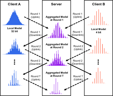
Figure 2: Quantization of a single client impacts weight distribution, affecting both the individual client and the global model, as well as clients operating at full precision.

Previous studies such as FedPAQ (Reisizadeh et al., 2020) and FedHQ (Chen et al., 2021) have used quantization in FL mainly to improve communication efficiency, whereas they have not fully addressed the associated performance decline. Achieving a balance between model performance and communication efficiency is challenging, as quantization can worsen weight distribution mismatches, particularly with low quantization bit lengths. Especially in FL, quantization effects accumulate over successive rounds as shown in Figure 2, potentially leading to more unstable and unpredictable training compared to non-quantized training due to the problem called distributional shift (Yoon et al., 2022).

In our research, we introduce FedShift, a novel approach designed to address communication efficiency and model performance challenges in the context of dual heterogeneity. We consider model quantization for the straggling clients while the full-precision model for other clients and tackle the model mismatch problem between different quantization levels to improve training efficiency and model performance.

In summary, we present the following major contributions:

• We proposed a simple yet effective weight-shifting algorithm to train mixed precision models in federated learning. The proposed algorithm does not require any additional information or data but only utilizes the uploaded clients’ model.

• We verify the performance improvement of the proposed algorithm through extensive experimental results. The additional improvement brought by FedShift is consistent over different baseline algorithms, different quantization levels, and various heterogeneous environments.

• We analyze the FedShift algorithm in terms of weight divergence analysis and convergence analysis. The weight shift effect is explained through weight divergence, and the conditions for the convergence of FedShift are presented.

2 Background and related works

This section provides an overview of FL. Then, we introduce relevant model quantization techniques, including uniform and non-uniform methods, and compare their advantages and disadvantages.

2.1 Federated Learning

The general FL optimization process can be formulated as follows:

$$\min_{\mathbf{w}}F(\mathbf{w})\triangleq\sum_{k=1}^{N}p_{k}F_{k}(\mathbf{w})$$ (1)

where $\min_{\mathbf{w}}$ represents the minimization operation over the parameter vector $\mathbf{w}$. $F(\mathbf{w})$ is the global objective function to be minimized. $N$ is the total number of federated clients or participants. In case of partial participation, we can set participation ratio $C$ for client selection, then total number of clients would be $\frac{N}{C}$. $p_{k}$ is the weight or contribution of client $k$ to the global objective. The local objective function for client $k$ is defined as:

$$F_{k}(\mathbf{w})\triangleq\frac{1}{n_{k}}\sum_{j=1}^{n_{k}}\ell(\mathbf{w};\xi_{k,j}).$$ (2)

where $F_{k}(\mathbf{w})$ is the local objective function for client $k$. $\frac{1}{n_{k}}$ represents the average operation over the data samples of client $k$. $\sum_{j=1}^{n_{k}}$ denotes the summation over the $n_{k}$ data samples of client $k$. $\ell(\mathbf{w};\xi_{k,j})$ is the loss or cost associated with the model parameter vector $\mathbf{w}$ and the $j$-th data sample $\xi_{k,j}$ of client $k$. Each client updates its weights using gradient descent based update algorithms, e.g., stochastic gradient descent (SGD), to minimize the loss function for $E$ local epochs in a round and completes the training after total $T$ rounds of aggregation.

Algorithm 1 Algorithm for FedAvg

0:  $N,C,T,E,\mathbf{w}^{0}$

1:  for $t=0,\dots,T-1$ do

2:     Server:

3:     Selects $N$ clients (set $\mathbb{N}_{t}$) with participation ratio $C$

4:     Sends $\mathbf{w}^{t}$ to all chosen devices

5:     Clients:

6:     Each chosen device $k\in\mathbb{N}_{t}$ updates $\mathbf{w}^{t}$ via SGD algorithm for $E$ epochs to obtain $\mathbf{w}^{t+1}_{k}$

7:     Sends back to the server

8:     Server:

9:     $\mathbf{w}^{t+1}$ = $\frac{1}{N}\sum_{k\in\mathbb{N}_{t}}\mathbf{w}_{k}^{t+1}$

10:  end for

The FedAvg algorithm, presented in Algorithm 1, is designed to enable multiple devices to update weights independently in FL. However, despite this decentralization, the central server remains the bottleneck during model aggregation, as it aggregates the models synchronously. Consequently, the slowest client, a straggler, determines the training time of each round($t$). In particular, since the uplink speed is generally slower than the downlink (Konečnỳ et al., 2016), letting the straggler to send quantization model would mitigate the straggler effect.

2.2 Model Quantization

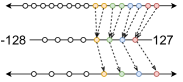
(a) 8-bit

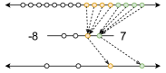
(b) 4-bit

Figure 3: Illustration of quantization and dequantization process with various bit widths

Quantization is a technique that reduces the precision of values from higher bits (high precision) to lower bits (low precision), aiming to preserve as much expressiveness of each value as possible. When it comes to model quantization in machine learning, we apply this method to the model’s weights to reduce the model size and enhance the inference speed. As illustrated in Figure 3, quantization and dequantization involve mapping the values to their closest counterparts. Quantization methods can be broadly categorized into uniform quantization and non-uniform quantization. Each method differs in how it approaches the mapping to achieve the most similar value representation (Gholami et al., 2021).

Uniform quantization is a method of remapping values from the original intervals into evenly spaced and smaller intervals. One of the well-known uniform quantization methods is called range-based asymmetric quantization (ASYM) (Guan et al., 2019), as shown in Equation 3. The process for dequantization can be derived simply by employing the inverse of the formula as demonstrated in Equation 4.

$$Q(w)=round(\frac{w-w_{min}}{w_{max}-w_{min}}*(2^{n}-1))$$ (3)

$$\tilde{w}=Q(w)*(\frac{w_{max}-w_{min}}{2^{n}-1})+w_{min}$$ (4)

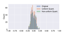
(a) Epoch: 0

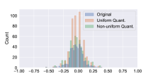
(b) Epoch: 4

Figure 4: The effect of 4-bit quantization techniques on the weight distribution over epochs during a single neural network training process.

ASYM quantization stands out for its straightforwardness and computational efficiency, with a $O(1)$ complexity. However, this method, which relies on identifying the maximum and minimum values, might not be suitable for data with non-uniform distributions where density varies. This is depicted in Figure 4, highlighting the drawbacks of uniform quantization (red bars). Typically, the distribution of weights in a neural network broadens as training progresses. Therefore, when quantization is based on the extreme values ($w_{min}$, $w_{max}$), the weights concentrated in the middle tend to cluster even more, exacerbating the deviation from the original distribution (blue bars). This effect becomes increasingly prominent when the target number of bits is small.

Algorithm 2 K-means-based Quantization

Quantization(Q):

Input: Weights $\mathbf{w}$, number of bits $\mathcal{N}$

Output: Quantized weights $qw$, codebook $cb$

1:  Compute centroids and cluster IDs using K-means clustering algorithm with $2^{\mathcal{N}}$ centroids and weights $w$

2:  Set codebook $cb$ to be the centroids

3:  Assign the closest centroid ID to each weight to generate the quantized weights $qw$

Dequantization(DeQ):

Input: Quantized weights $qw$, codebook $cb$

Output: Dequantized weights $\tilde{w}$

1:  Map $qw$ back to dequantized weights $\tilde{w}$ using $cb$

Non-uniform quantization methods adopt a more advanced strategy that accounts for the distribution of values when assigning them to smaller intervals. This contrasts with uniform quantization, which overlooks value density and can lead to an outlier effect. A solution to this issue is the use of K-means clustering for interval determination (Gong et al., 2014; Wu et al., 2016). K-means clustering requires specifying the number of clusters, which is equal to two the power of a number of bits in this context. Algorithm 2 clusters a one-dimensional data set (the flattened model weights) and computes $2^{\mathcal{N}}$ centroids to represent the interval values. Using K-means clustering, this quantization method lessens the influence of extreme weight values, as depicted by the green bars in Figure 4(b). However, K-means clustering comes with higher computational demands, having a complexity of $O(n^{2})$, where $n$ is the number data point.

3 Proposed Method

This section presents our proposed method in terms of both the system architecture and algorithm. The system architecture outlines a way of integrating the quantization process into the existing training workflow, while the algorithm details a strategy for minimizing performance degradation within our experimental setting.

3.1 System architecture

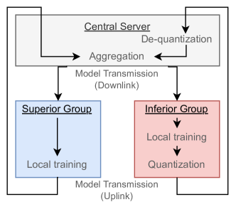
Figure 5: Training flow with inferior group incorporating quantization process

Figure 5 demonstrates how, in the process of conventional FL training, certain clients implement quantization during the model transmission phase. In our client setting, we assume that clients with subpar network conditions have been identified and categorized into two groups as follows: inferior and superior, based on the quality of their network environment.

In our training flow, clients of the superior group follow the standard FedAvg flow. As their network speed is sufficient, it is unnecessary to quantize their model. Conversely, quantization is applied to the inferior group. Hence, the algorithm operates differently depending on the group in question. Upon receiving the model from the central server, the inferior group starts training and quantizes the trained weights. These quantized weights are then transmitted to the central server. Suppose the received model parameters are from the superior group. In that case, they are utilized as is, whereas if they are from the inferior group, the central server employs the provided information to perform dequantization. These dequantization and weight aggregation methods follow the proposed FedShift algorithm.

3.2 FedShift - Weight Shifting Aggregation

Since we apply model quantization to reduce the uplink transmission time from clients to the central server, dequantization is used in the central server to be aggregated as 32-bit values. Thus, the iterative process of quantization and dequantization can cause continuous changes in the model’s weight distribution and can significantly diverge from the distribution of weight values it should have. This issue has a more pronounced impact on model performance as the number of quantization bits decreases, leading us to recognize the necessity for a solution to mitigate the disparity between the superior and inferior models. Motivated by weight normalization (Salimans & Kingma, 2016; Huang et al., 2017) and weight standardization (Qiao et al., 2019) techniques commonly used in traditional machine learning approaches, we have devised our novel method.

First, we need to note that the following equations describe the weight within a layer of the neural network model. Let $m^{t+1}=\frac{1}{P}\sum_{p}\mathbf{w}^{t+1}[p]$ be the average of the weights of all clients (inferior$+$superior) at round $t+1$. The client sets $\mathbb{I}$ and $\mathbb{S}$ denotes the inferior and superior clients selected at each round, and let $I$ and $S$ be the number of clients in each set, respectively. The calculation of $m^{t+1}$ is given by the following equation:

$$m^{t+1}=\frac{1}{P(I+S)}\sum_{p}\left(\sum_{i\in\mathbb{I}}\mathbf{w}_{i}^{t+1}[p]+\sum_{j\in\mathbb{S}}\mathbf{w}_{j}^{t+1}[p]\right)$$ (5)

where $p$ is the index of weight in the layer, $P$ is the total number of weights and $\mathbf{w}_{i}^{t+1}[p]$ and $\mathbf{w}_{j}^{t+1}[p]$ represent the weights of inferior clients and superior clients, respectively.

The weights of inferior clients $i\in\mathbb{I}$ are shifted by subtracting the value $m^{t+1}$. The shifted weight for each inferior client $i$ is calculated as follows:

$${\mathbf{w}_{i}^{t+1}}^{\prime}=\mathbf{w}_{i}^{t+1}-m^{t+1}\vec{\mathbf{1}}_{P},\hskip 14.22636pt\forall i\in\mathbb{I}$$ (6)

The updated weight of the global model at round $t+1$ is calculated by taking the shifted weights of the inferior clients and the original weights of the superior clients as below. Note that the number of chosen clients $N$ is equal to $I+S$.

$$\mathbf{w}^{t+1}[p]=\frac{1}{N}\left(\sum_{i\in\mathbb{I}}{\mathbf{w}_{i}^{t+1}}^{\prime}[p]+\sum_{j\in\mathbb{S}}\mathbf{w}_{j}^{t+1}[p]\right)$$ (7)

Ultimately, the above shifting process can be simplified as follows:

$$\hat{\mathbf{w}}^{t+1}_{FS}=\mathbf{w}^{t+1}-\frac{I}{N}m^{t+1}\vec{\mathbf{1}}_{P}.$$ (8)

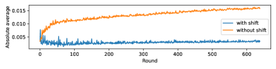
Figure 6: Change in the average absolute weight value over time, determined by the presence (blue) or absence (orange) of shifting during training rounds.

The purpose of shifting the weights is to prevent the quantized weights from diverging over the rounds. In our in-depth analysis of the FedShift algorithm, we observed a consistent anomaly in the weight distribution of models during the FL rounds, specifically during the quantization processes. As the rounds progressed, the weight distribution of models exhibiting suboptimal performance exhibited a skewness, as shown in Figure 6. This skewness can be attributed to a high concentration of values within a specific range during quantization. To mitigate this, we propose leveraging the weight distribution of the optimally trained models (full precision) as a reference. Our approach involves shifting the weights of the suboptimal models between 0 and the average weight of the optimal models, as shown in Figure 7.

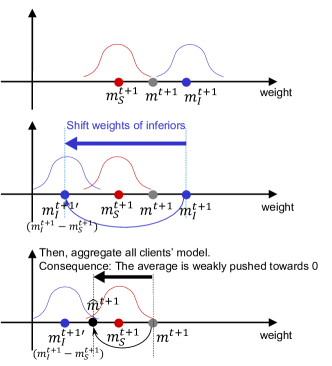
Figure 7: Concept visualization of FedShift

If we examine the result of shifting, it pushes the average weight to 0 with the proportion of $S/N$, which is the ratio of superior clients to all clients. It can be easily seen by examining the average of shifted weight as follows.

$$\begin{array}[]{l}\displaystyle\hat{m}^{t+1}=\frac{1}{PK}\left(\sum_{p=1}^{P}\sum_{k=1}^{N}{(w_{k}^{t+1}}[p]-\frac{I}{N}m^{t+1})\right)\\ \displaystyle=m^{t+1}-\frac{I}{N}m^{t+1}=\frac{S}{N}m^{t+1}.\end{array}$$ (9)

Since $\mathbb{S}$ is the subset of $\mathbb{N}$, $0<|\hat{m}^{t+1}|<|m^{t+1}|$ holds.

Algorithm 3 Algorithm for FedShift

0:  $N,C,T,E,\mathbf{w}^{0},\mathcal{N}$

1:  for $t=0,\dots,T-1$ do

2:     Server:

3:     Selects $N$ devices (set $\mathbb{N}_{t}$) with participation ratio $C$

4:     Sends $w^{t}$ to all chosen devices

5:     Clients:

6:     Chosen devices $k\in\mathbb{N}_{t}$ update $\mathbf{w}_{k}^{t}$ for $E$ epochs to obtain $\mathbf{w}^{t+1}_{k}$ and auxiliary data $\chi^{t+1}_{k}$ for DeQ.

7:     if $k\in I$ then

8:        $qw_{i}^{t+1}$, $\chi_{i}^{t+1}$ = $Q(w_{k}^{t+1},\mathcal{N})$

9:     else if $k\in S$ then

10:        $\mathbf{w}_{j}^{t+1}$ = $\mathbf{w}_{k}^{t+1}$

11:     end if

12:     Sends back to the server

13:     Server:

14:     $\mathbf{w}_{i}^{t+1}=DeQ(qw_{i}^{t+1}$, $\chi_{i}^{t+1}),\hskip 14.22636pt\forall i\in\mathbb{I}$

15:     $m^{t+1}=\frac{1}{P(I+S)}\sum\limits_{p}\left(\sum\limits_{i\in\mathbb{I}}w_{i}^{t+1}[p]+\sum\limits_{j\in\mathbb{S}}\mathbf{w}_{j}^{t+1}[p]\right)$

16:     $\hat{\mathbf{w}}^{t+1}_{FS}=\mathbf{w}^{t+1}-\frac{I}{N}m^{t+1}\vec{\mathbf{1}}_{P}$

17:  end for

As depicted in Algorithm 3, FedShift incorporates two steps to match the weight’s distribution. The first step involves computing the mean value ($m$) of all the weights. Then, this mean value is subtracted solely from the weights of the inferior models. Then, the weights for the global model are obtained through an averaging step.

Convergence Analysis

Here, we present the result of the convergence analysis of FedShift as the following theorem. It implies that when the average of weights, $M$, goes to $0$, FedShift algorithm converges to the solution with the convergence rate of $\mathcal{O}(\frac{1}{T})$. This finding is in accordance with the simulation results in which the average of weights becomes very close to $0$ and shows stable training with FedShift.

Theorem 1.

Under the Assumptions 1 to 5 regarding $L$-smoothness & $\mu$-convexity of function and bounded gradients and weight average, for the choice of $\beta=\frac{2}{\mu}$, $\gamma=\max\{\frac{8L}{\mu},E\}-1$, $\varepsilon>0$, then $\eta_{\tau}=\frac{2}{\mu}\frac{1}{\gamma+\tau}$, the error after $\tau$ local steps of update with full client participation satisfies

$$\mathbb{E}[F(\overline{\mathbf{w}}_{\tau})]-F^{*}$$

$$\leq\underbrace{\frac{L}{2}\frac{1}{\tau+\gamma}\left(\frac{B_{1}\beta^{2}}{\left(1+\frac{1}{\varepsilon}\right)\beta\mu-\frac{1}{\varepsilon}\left(\tau+\gamma\right)-1}+(\gamma+1)\Delta_{1}\right)}_{\text{Vanishing term}}$$

$$+\underbrace{\frac{L}{2}\left(\frac{B_{2}M}{\left(1+\frac{1}{\varepsilon}\right)\beta\mu\frac{1}{\tau+\gamma}-\frac{1}{\varepsilon}-\frac{1}{\tau+\gamma}}\right)}_{\text{Vanishes when $M\rightarrow 0$}}$$

where $B_{1}$, $B_{2}$ and $M$ are values determined by bounds, $F^{*}$ is the minimum point of function $F$, and $\Delta_{\tau=1}=\mathbb{E}\|\overline{\mathbf{w}}_{\tau=1}-\mathbf{w}^{*}\|^{2}$

Proof.

See Appendix A for the detailed proof and notations. ∎

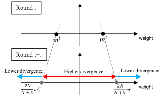
Figure 8: Illustration of FedShift balancing divergence

Divergence Analysis In another aspect, we provide an analysis of the divergence of the model between the rounds. We examine how much the global model diverges from the previous round by comparing it with the baseline algorithm FedAvg. The model divergence from the previous round to the current round is considered one of the measures of stable FL training (Rehman et al., 2023). If divergence is too large between rounds, it may ruin the collaboration between clients, but too small divergence would result in slow training. It turns out that FedShift balances the divergence between rounds based on the average weight of the previous and current rounds, i.e., $m^{t}$, $m^{t+1}$. Figure 8, shows that depending on the $m^{t}:m^{t+1}$ ratio, the divergence differs. The result is summarized in the following theorem. We encourage the readers to refer to the appendix for detailed proof and interpretations with examples.

Theorem 2.

Let $D$ be the L2 divergence from the previous round global model to the current round global model. Then, the divergence of FedShift and Fedavg satisfies the following condition

$$\displaystyle D_{FA}^{2}-D_{FS}^{2} =\frac{IP}{N}\left(\frac{N+S}{N}(m^{t+1})^{2}-2\frac{m^{t}}{(m^{t+1})^{2}}\right)$$ (10)

Proof.

See Appendix B for the detailed proof and interpretations. ∎

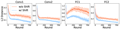
Figure 9: L2 distance for each layer between the global model at round $t-1$ and the inferior model at round $t$ over 800 rounds

In Figure 9, we evaluated the effectiveness of FedShift by assessing the L2 distance between the aggregated weights of inferior clients at round $t$ and the global model’s weights from the previous round($t-1$). The graph illustrates that during the shifting process, all layers exhibit a reduced L2 distance between the previous global model and the inferior models. With continued learning, the model divergence, which initially resulted from quantization side effects, gradually diminishes. This observation supports the successful functioning of the technique. Consequently, we can infer that FedShift promotes more stable training progression with minimal disruptions.

4 Experiment and Result

This section describes our experiment, including the dataset, relevant models, and FL environment settings. Then, performance evaluations of our proposed FedShift algorithm and other conventional algorithms are presented in various aspects. The source code can be found in our repository.

4.1 Dataset

(a) Superior group

(b) Inferior group

Figure 10: Data partitioning with inferior and superior group

We use the CIFAR10 dataset (Krizhevsky et al., ) for our main experiment. 50,000 images are used for training, and 10,000 images are used for testing on the central server, focusing on measuring the top-1 accuracy of the global model. To accommodate our non-IID dataset setting and replicate a scenario of dual heterogeneity, we organize the dataset into customized shard partitions. Specifically, we initially segregate the dataset into two distinct groups, ensuring the superior and inferior groups do not share any labels. For convenience, we put the even number of labels into the superior group and the odd number into the inferior group. Then, each client holds two classes within their group data, as shown in Figure 10.

4.2 Backbone Model and FL Setting

The architecture of our model is based on a Convolutional Neural Network (CNN) similar to the one presented in (McMahan et al., 2017), which includes two convolutional layers with max-pooling layers and two fully connected layers. The optimizer used for training is Stochastic Gradient Descent (SGD), with a learning rate of 0.005 and a momentum of 0.9. The network weights are initialized using Kaiming initialization. Our primary experiment configured a setup with 100 clients and utilized a dataset partitioned into 1000 subsets according to our data partitioning strategy. A random fraction ($C$) of 0.1 is selected for client participation in each training round. The experiment is structured to run for 800 training rounds ($T$). Each client’s local batch size is determined to be 50 with 10 local epochs ($E$). Moreover, we conduct a comparative analysis of three widely used FL algorithms – FedAvg, FedProx, and SCAFFOLD (Karimireddy et al., 2020) – both with and without the integration of the FedShift technique. We explore the impact of quantization on the performance of our system by examining five different bit widths, ranging from 4 to 8 bits. Regarding quantization techniques, we evaluate two methods: ASYM quantization as a uniform quantization and K-means clustering-based non-uniform quantization. We then apply our FedShift method to both quantization techniques to demonstrate its effectiveness.

More experiments with different datasets, such as CIFAR-100, and different distributions, such as Dirichlet, are included in the Appendix C.

4.3 Evaluation

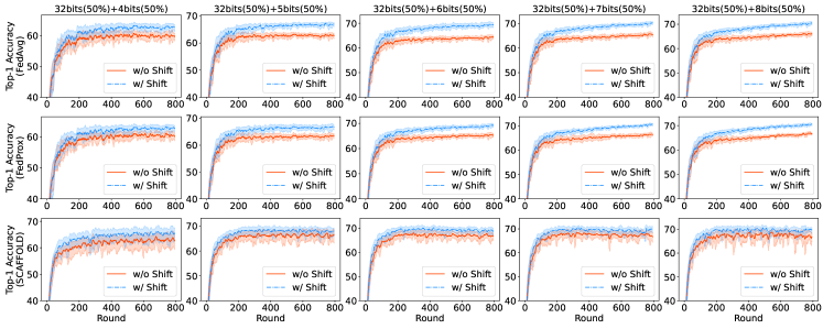
Figure 11: Performance comparison of three FL algorithms across various bit widths, with and without shift aggregation. Each graph represents the top-1 accuracy smoothed using a simple moving average with a window of 10 rounds. The experiments cover 50% usage of 32-bit width combined with 50% of 4, 5, 6, 7, and 8-bit widths by non-uniform quantization.

Models	32+32bit	Shifting	Uniform Quantization
			32+4bit		32+5bit		32+6bit		32+7bit		32+8bit
FedAvg	66.20$\pm$1.98	w/o Shift	N/A	-	54.1$\pm$3.05	+4.2	63.4$\pm$1.53	+3.1	66.4$\pm$0.84	+3.4	66.8$\pm$0.80	+3.7
		w/ Shift	N/A		58.3$\pm$2.70	$\sigma$:$\downarrow$11%	66.4$\pm$1.11	$\sigma$:$\downarrow$27%	69.8$\pm$1.02	$\sigma$:$\uparrow$21%	70.5$\pm$0.74	$\sigma$:$\downarrow$8%
FedProx	66.22$\pm$1.37	w/o Shift	N/A	-	44.6$\pm$5.47	+13.0	64.8$\pm$1.25	+2.1	66.2$\pm$1.41	+3.8	66.7$\pm$0.96	+3.3
		w/ Shift	N/A		57.6$\pm$2.26	$\sigma$:$\downarrow$59%	66.9$\pm$1.08	$\sigma$:$\downarrow$14%	70.0$\pm$1.01	$\sigma$:$\downarrow$28%	70.0$\pm$0.77	$\sigma$:$\downarrow$20%
SCAFFOLD	65.98$\pm$2.67	w/o Shift	N/A	-	44.4$\pm$9.19	+11.1	63.8$\pm$4.01	+3.0	68.2$\pm$1.12	+1.8	67.5$\pm$1.37	+2.9
		w/ Shift	N/A		55.5$\pm$3.80	$\sigma$:$\downarrow$59%	66.8$\pm$2.69	$\sigma$:$\downarrow$33%	70.0$\pm$1.21	$\sigma$:$\uparrow$8%	70.4$\pm$1.72	$\sigma$:$\uparrow$26%
Models	32+32bit	Shifting	Non-uniform Quantization
			32+4bit		32+5bit		32+6bit		32+7bit		32+8bit
FedAvg	66.20$\pm$1.98	w/o Shift	59.7$\pm$1.34	+2.8	62.7$\pm$1.06	+4.2	64.3$\pm$0.94	+5.0	65.4$\pm$0.97	+4.8	66.0$\pm$0.92	+4.4
		w/ Shift	62.5$\pm$1.29	$\sigma$:$\downarrow$4%	66.9$\pm$0.89	$\sigma$:$\downarrow$16%	69.3$\pm$1.11	$\sigma$:$\uparrow$18%	70.2$\pm$0.75	$\sigma$:$\downarrow$23%	70.4$\pm$0.84	$\sigma$:$\downarrow$9%
FedProx	66.22$\pm$1.37	w/o Shift	60.1$\pm$1.33	+2.5	63.5$\pm$0.94	+3.1	65.2$\pm$0.89	+3.8	66.4$\pm$0.73	+4.1	66.6$\pm$0.58	+3.9
		w/ Shift	62.6$\pm$1.16	$\sigma$:$\downarrow$13%	66.6$\pm$0.97	$\sigma$:$\uparrow$3%	69.0$\pm$0.73	$\sigma$:$\downarrow$18%	70.5$\pm$0.63	$\sigma$:$\downarrow$14%	70.5$\pm$0.62	$\sigma$:$\uparrow$7%
SCAFFOLD	65.98$\pm$2.67	w/o Shift	62.9$\pm$1.98	+3.0	66.5$\pm$2.68	+1.4	66.9$\pm$1.43	+1.9	66.7$\pm$1.82	+3.0	66.8$\pm$1.67	+3.1
		w/ Shift	65.9$\pm$1.53	$\sigma$:$\downarrow$23%	67.9$\pm$1.56	$\sigma$:$\downarrow$42%	68.8$\pm$1.34	$\sigma$:$\downarrow$6%	69.7$\pm$1.48	$\sigma$:$\downarrow$19%	69.6$\pm$1.50	$\sigma$:$\downarrow$10%

Table 1: Summary of federated learning algorithm performance with different quantization strategies. The table shows the baseline accuracy for 32+32 bit (no quantization) and the final performance with uniform and non-uniform quantization across various bit widths.

Baseline Performance After training our three baseline algorithms using the current dataset configuration, backbone model, and federated learning parameters in a full-precision state without quantization, we observed the following performance scores: FedAvg achieved 66.20%, FedProx achieved 66.22%, and SCAFFOLD reached 65.98% top-1 accuracy. These results signify the starting point of our performance evaluation. Next, we will examine how the performance metrics change when we introduce clients with quantization applied. The overall experiment result can be found in Figure 11 and Table 1.

Quantization Effect First, the most significant difference becomes apparent when divided by the quantization technique. In the case of uniform quantization, training was not completed properly in the 4-bit scenario. Conversely, training remained stable with non-uniform quantization even in the 4-bit scenario. One intriguing observation is that, contrary to the initial expectation that quantization would negatively impact model performance, starting from 7 bits, the performance was either similar to or better than that of baseline models trained with full precision. This suggests a phenomenon akin to some studies (Wu & Flierl, 2020) where quantization actually helps prevent overfitting by working as a regularization technique, as from 7 bits onward, the expressiveness of the original weight can be effectively preserved. At lower bit levels (4-6 bits), non-uniform quantization exhibited superior performance, while at 7-8 bits, uniform quantization demonstrated higher performance. This implies that when the number of expressible values is in the range of 128-256, the influence from weight outliers at the extremes becomes negligible.

Effect of Weight Shifting When we integrate weight shifting with each of the baseline algorithms as proposed, we observe that weight shifting consistently improves performance across all scenarios. Regardless of the bit precision or quantization technique, weight shifting increased performance by an average of 3.9%. Notably, it successfully enabled the training of models (FedProx, SCAFFOLD) that previously struggled with stable training, particularly in the case of uniform 5-bit quantization. This demonstrates that FedShift not only enhances performance but also contributes to a more stable overall training process.

Furthermore, this can be verified by examining the standard deviation of independently trained performance. In situations where weight shifting is applied, we observe lower standard deviation values compared to cases where no shifting is used, with the exception of scenarios where the standard deviation is close to 1.0. This indicates that FedShift can provide more consistent performance across various experimental conditions.

Bits	Weight	Quantization	Auxiliary	Computing
	Size		Data Size	Overhead
4bit	1,052KB	Uniform	0.25KB	10ms
		Non-uniform	6.19KB	179ms
8bit	2,105KB	Uniform	0.25KB	10ms
		Non-uniform	88.82KB	2,172ms
32bit	8,421KB	Apple M1 Pro, 8 Core, 16GB RAM

Table 2: Data size and quantization overhead measurements

Communication Efficiency Table 2 presents a comparison of different bit widths (4bit, 8bit, and 32bit) for parameter size in kilobytes (KB), the size of auxiliary data sent for dequantization in KB, and the computational overhead for quantization from each client in milliseconds (ms) based different quantization methods. When assessing the model parameter size, it is evident that the total size reduces as the bit count decreases. However, with uniform quantization, only the 32-bit maximum and minimum values need to be transmitted for dequantization, adding a mere 0.25KB. In contrast, non-uniform quantization requires transmitting each 32-bit centroid, increasing the size proportional to the number of bits. Taking into account the stability of training, the volume of data transmission, and computational overhead, it is advisable to employ uniform quantization for clients that possess a robust network environment, utilizing 8-bit quantization. Meanwhile, for clients that necessitate consideration of up to 4-bit quantization, applying the non-uniform quantization can be seen as a suitable approach. To determine when 4-bit non-uniform quantization is more efficient than 32-bit for communication, we consider weight transfer time and computing overhead at a 1MB/s network speed. With a 1,059KB data size (including auxiliary data) and 179ms computing delay for 4-bit quantization, the efficiency threshold ratio is about 7.78. This indicates that 4-bit quantization remains more efficient as long as its network speed is less than 7.78 times slower than 32-bit.

5 Conclusion

To conclude, this research has presented a novel aggregation method called FedShift, which addresses the challenge of reconciling quantized and non-quantized weights in FL in heterogeneous environments. We have explored a scenario where systems heterogeneity and statistical heterogeneity coexist, requiring a trade-off between a model’s performance and total training time. We have utilized model quantization to mitigate the impact of stragglers on training time. Furthermore, we have demonstrated that FedShift can minimize the performance degradation caused by quantization. Our simulation results suggest that FedShift can effectively match weight distributions between different precision models and improve the overall performance in a concurrent heterogeneous scenario.

Appendix A Convergence Analysis of FedShift

To show that the proposed FedShift algorithm converges with the convergence rate of $\mathcal{O}(\frac{1}{T})$, we provide convergence analysis on FedShift in full participation scenario. It should be noted that we follow the convergence analysis techniques that is used by (Li et al., 2019) which is also motivated by many existing literature on convergence analysis, i.e., local SGD convergence (Stich, 2018), FedProx (Li et al., 2018). Due to the nature of distributed clients, we consider that the data is distibuted non-IID among clients.

A.1 Problem formulation

The local objective function of the client $k$ is denoted as $F_{k}(\mathbf{w})$ and the baseline FedAvg algorithm has the global objective function as

$$\min_{\mathbf{w}}F(\mathbf{w})\triangleq\sum_{k=1}^{N}p_{k}F_{k}(\mathbf{w}).$$ (11)

The optimum value of $F$ and $F_{k}$ are denoted as $F^{*}$ and $F_{k}^{*}$ and corresponding optimum weights are denoted as $\mathbf{w}^{*}$ and $\mathbf{w}_{k}^{*}$respectively. Also, $p_{k}$ is the aggregation weight of the client $k$ where $\sum_{k=1}^{N}p_{k}=1$, since we consider the full participation for the convergence analysis. Otherwise, the sum of participating clients’ aggregation weights at each round should be 1. In order to analyze the model parameter update, we break down into steps within a round. The update of local weight at step $\tau$ can be expressed as follows.

$$\mathbf{w}_{k}^{\tau+1}=\mathbf{w}_{k}^{\tau}-\eta_{\tau}\nabla F_{k}(\mathbf{w}_{k}^{\tau},\xi_{k}^{\tau})$$ (12)

For the sequence $\tau=0,1,2,\dots$ and the global synchronization step, $\mathcal{I}_{E}=\{nE|n=1,2,\cdots\}$, the weights are uploaded to server only when $\tau+1\in\mathcal{I}_{E}$. For convenience, we let $\overline{\mathbf{w}}_{\tau}=\sum_{k=1}^{N}p_{k}\mathbf{w}_{k}^{\tau}$, $g_{\tau}=\sum_{k=1}^{N}p_{k}\nabla F_{k}(\mathbf{w}_{k}^{\tau},\xi_{k}^{\tau})$ and $\overline{\mathbf{g}}_{\tau}=\sum_{k=1}^{N}p_{k}\nabla F_{k}(\mathbf{w}_{k}^{\tau})$, thus $\mathbb{E}[\mathbf{g}_{\tau}]=\overline{\mathbf{g}}_{\tau}$.

Notations:

$$\mathbf{w}_{k}^{\tau} :\text{ Client }k\text{'s model weight at step }\tau$$

$$\xi_{k}^{\tau} :\text{ Client }k\text{'s sampled data at step }\tau$$

$$\eta_{\tau} :\text{ Learning rate at step }\tau$$

$$m_{\tau+1} :\text{ mean of global weights before shift, i.e., }\mathbb{E}[W_{t}-\eta_{t}\overline{\mathbf{g}}_{\tau}]$$

$$\alpha :I/N\text{ the ratio of inferior clients,}\text{ where }I\text{: Number of inferior clients, }N\text{: Total number of clients}$$

$$p_{k} :\text{aggregation weight for client $k$}$$

$$\vec{\mathbf{1}}_{P} :\text{$P$-sized vector with every element 1 where $P$ is the number of weight parameter in $\mathbf{w}$}$$

We have the following assumptions on the functions $F_{1},\cdots,F_{N}$ where Assumptions 1 and 2 are standard and Assumptions 3 and 4 are also typical which have been made by the works (Zhang et al., 2012), (Stich, 2018) and (Yu et al., 2019).

Assumption 1.

L-Smoothness: For all $\mathbf{w}$ and $\mathbf{w^{\prime}}$, $F_{k}(\mathbf{w})\leq F_{k}(\mathbf{w^{\prime}})+(\mathbf{w}-\mathbf{w^{\prime}})^{\intercal}\nabla F_{k}(\mathbf{w^{\prime}})+\frac{L}{2}||\mathbf{w}-\mathbf{w^{\prime}}||_{2}^{2}$

Assumption 2.

$\mu$-strongly convex: For all $\mathbf{w}$ and $\mathbf{w^{\prime}}$, $F_{k}(\mathbf{w})\geq F_{k}(\mathbf{w^{\prime}})+(\mathbf{w}-\mathbf{w^{\prime}})^{\intercal}\nabla F_{k}(\mathbf{w^{\prime}})+\frac{\mu}{2}||\mathbf{w}-\mathbf{w^{\prime}}||_{2}^{2}$

Assumption 3.

Variance of gradients are bounded: Let $\xi_{t}^{k}$ be the data ramdomly sampled from k-th client’s data. The variance of stochastic gradients in each device is bounded as: $\mathbb{E}[||\nabla F_{k}(\mathbf{w}_{k}^{\tau},\xi_{k}^{\tau})-\nabla F_{k}(\mathbf{w}_{k}^{\tau})||_{2}^{2}]\leq\sigma_{k}^{2}$ for $k=1,\cdots,N$

Assumption 4.

Stochastic gradients are bounded: $\mathbb{E}\left[||\nabla F_{k}(\mathbf{w}_{k}^{\tau},\xi_{k}^{\tau})||_{2}^{2}\right]\leq G^{2}$ for $k=1,\cdots,N$ and $\tau=1,2,\cdots$

Here, we have additional assumption regarding the weight distribution of training model. This is a reasonable assumption because FL training would converge at some point then average of model’s weights does not diverge to positive/negative infinity unless gradient explodes.

Assumption 5.

Weight average is bounded: $\mathbb{E}\left[m^{2}_{\tau}\right]\leq M$ for all $\tau$

A.2 Key Lemmas

We first establish these Lemmas to be used in the proof of Theorem 1.

Lemma 1.

Assuming that Assumption 3 holds and if $\eta_{\tau}\leq\frac{1}{4L}$, following inequality holds.

$$\mathbb{E}[\|\overline{\mathbf{w}}_{\tau+1}-\mathbf{w}^{*}\|^{2}] \leq\left(1+\frac{1}{\varepsilon}\right)\left((1-\eta_{\tau}\mu)\mathbb{E}[\|\overline{\mathbf{w}}_{\tau}-\mathbf{w}^{*}\|^{2}]+6L\eta_{\tau}^{2}\Gamma+2\mathbb{E}\left[\sum_{k=1}^{N}p_{k}\|\overline{\mathbf{w}}_{\tau}-\mathbf{w}_{k}^{*}\|^{2}\right]\right)$$

$$\quad+\eta_{\tau}^{2}\mathbb{E}[\|\mathbf{g}_{\tau}-\overline{\mathbf{g}}_{\tau}\|^{2}]+\left(1+\varepsilon\right)\|\vec{\mathbf{1}}_{P}\|^{2}\mathbb{E}[(\alpha m_{t+1})^{2}]$$

We recall Lemma 2 and 3 of (Li et al., 2019) as follows.

Lemma 2.

Assuming that Assumption 3 holds, it follows that

$$\mathbb{E}[\left\|\mathbf{g}_{\tau}-\overline{\mathbf{g}}_{\tau}\right\|^{2}]\leq\sum_{k=1}^{N}p_{k}^{2}\sigma_{k}^{2}.$$ (13)

Lemma 3.

Assuming that Assumption 4 holds and $\eta_{\tau}$ is non-increasing and $\eta\leq 2\eta_{t+E}$ for all $t$, the following inequality satifies.

$$\mathbb{E}\left[\sum_{k=1}^{N}p_{k}\left\|\overline{\mathbf{w}}_{\tau}-\mathbf{w}_{k}^{t}\right\|^{2}\right]\leq 4\eta_{\tau}^{2}(E-1)^{2}G^{2}$$ (14)

A.3 Proof of Lemma 1

Proof.

We have global update rule for FedShift as $\overline{\mathbf{w}}_{\tau+1}=\overline{\mathbf{w}}_{\tau}-\eta_{\tau}\overline{\mathbf{g}}_{\tau}-\alpha m_{\tau+1}\vec{\mathbf{1}}_{P}$, therefore,

$$\|\overline{\mathbf{w}}_{\tau+1}-\mathbf{w}^{*}\|^{2} =\|\overline{\mathbf{w}}_{\tau}-\eta_{\tau}\mathbf{g}_{\tau}-\alpha m_{\tau+1}\vec{\mathbf{1}}_{P}-\mathbf{w}^{*}\|^{2}$$

$$=\|\overline{\mathbf{w}}_{\tau}-\mathbf{w}^{*}-\eta_{\tau}\mathbf{g}_{\tau}-\alpha m_{\tau+1}\vec{\mathbf{1}}_{P}-\eta_{\tau}\overline{\mathbf{g}}_{\tau}+\eta_{\tau}\overline{\mathbf{g}}_{\tau}\|^{2}$$

$$=\underbrace{\|\overline{\mathbf{w}}_{\tau}-\mathbf{w}^{*}-\eta_{\tau}\overline{\mathbf{g}}_{\tau}-\alpha m_{\tau+1}\vec{\mathbf{1}}_{P}\|^{2}}_{Q_{1}}+\eta_{\tau}^{2}\|\mathbf{g}_{\tau}-\overline{\mathbf{g}}_{\tau}\|^{2}$$

$$\quad+\underbrace{2\eta_{\tau}\langle\overline{\mathbf{w}}_{\tau}-\mathbf{w}^{*}-\eta_{\tau}\overline{\mathbf{g}}_{\tau}-\alpha m_{\tau+1}\vec{\mathbf{1}}_{P},\mathbf{g}_{\tau}-\overline{\mathbf{g}}_{\tau}\rangle}_{Q_{2}}$$

According to Lemma 2, the second term on RHS is bounded as $\eta_{\tau}^{2}\|\mathbf{g}_{\tau}-\overline{\mathbf{g}}_{\tau}\|^{2}\leq\eta_{\tau}^{2}\sum_{k=1}^{N}p_{k}^{2}\sigma_{k}^{2}$. Note that when we take expectation, $\mathbb{E}[Q_{2}]=0$ due to unbiased gradient.

Then, We expand $Q_{1}$

$$Q_{1} =\|\overline{\mathbf{w}}_{\tau}-\mathbf{w}^{*}-\eta_{\tau}\overline{\mathbf{g}}_{\tau}-\alpha m_{\tau+1}\vec{\mathbf{1}}_{P}\|^{2}$$ (15)

$$=\underbrace{\|\overline{\mathbf{w}}_{\tau}-\mathbf{w}^{*}-\eta_{\tau}\overline{\mathbf{g}}_{\tau}\|^{2}}_{A_{1}}+(\alpha m_{\tau+1})^{2}\|\vec{\mathbf{1}}_{P}\|^{2}-2\langle\overline{\mathbf{w}}_{\tau}-\mathbf{w}^{*}-\eta_{\tau}\overline{\mathbf{g}}_{\tau},\alpha m_{\tau+1}\vec{\mathbf{1}}_{P}\rangle$$ (16)

$$=A_{1}+(\alpha m_{\tau+1})^{2}\|\vec{\mathbf{1}}_{P}\|^{2}-2\langle\overline{\mathbf{w}}_{\tau}-\mathbf{w}^{*}-\eta_{\tau}\overline{\mathbf{g}}_{\tau},\alpha m_{\tau+1}\vec{\mathbf{1}}_{P}\rangle$$ (17)

$$\leq A_{1}+\frac{1}{\varepsilon}A_{1}+\varepsilon(\alpha m_{\tau+1})^{2}\|\vec{\mathbf{1}}_{P}\|^{2}+(\alpha m_{\tau+1})^{2}\|\vec{\mathbf{1}}_{P}\|^{2}$$ (18)

$$=\left(1+\frac{1}{\varepsilon}\right)A_{1}+\left(1+\varepsilon\right)(\alpha m_{\tau+1})^{2}\|\vec{\mathbf{1}}_{P}\|^{2}$$ (19)

where inequality (18) is due to a useful inequality property as follows.

$$\text{(by AM-GM, Cauchy-Schwartz, }\epsilon>0):$$

$$-2\langle a,b\rangle\leq\epsilon\|a\|^{2}+\epsilon^{-1}\|b\|^{2}\quad$$

which make the cross term on RHS satisfy the inequality below

$$-2\langle\overline{\mathbf{w}}_{\tau}-\mathbf{w}^{*}-\eta_{\tau}\overline{\mathbf{g}}_{\tau},\alpha m_{\tau+1}\vec{\mathbf{1}}_{P}\rangle$$

$$\leq\frac{1}{\varepsilon}\|\overline{\mathbf{w}}_{\tau}-\mathbf{w}^{*}-\eta_{\tau}\overline{\mathbf{g}}_{\tau}\|^{2}+\varepsilon(\alpha m_{\tau+1})^{2}\|\vec{\mathbf{1}}_{P}\|^{2}.$$

Then, $A_{1}$ is known to be bounded as follows (see (Li et al., 2019) for detailed proof).

$$A_{1} \leq\left(1-\mu\eta_{\tau}\right)\|\overline{\mathbf{w}}_{\tau}-\mathbf{w}^{*}\|^{2}+2\sum_{k=1}^{N}\|\overline{\mathbf{w}}_{\tau}-\mathbf{w}_{k}^{*}\|^{2}+6\eta_{\tau}^{2}L\Gamma$$

Therefore, writing above inequalities and Lemma 2 and 3 all together, we have

$$\mathbb{E}[\|\overline{\mathbf{w}}_{t+1}-\mathbf{w}^{*}\|^{2}] \leq\left(1+\frac{1}{\varepsilon}\right)\left((1-\eta_{\tau}\mu)\mathbb{E}[\|\overline{\mathbf{w}}_{\tau}-\mathbf{w}^{*}\|^{2}]+6L\eta_{\tau}^{2}\Gamma+2\mathbb{E}\left[\sum_{k=1}^{N}p_{k}\|\overline{\mathbf{w}}_{\tau}-\mathbf{w}_{k}^{*}\|^{2}\right]\right)$$

$$\quad+\eta_{\tau}^{2}\mathbb{E}[\|\mathbf{g}_{\tau}-\overline{\mathbf{g}}_{\tau}\|^{2}]+\left(1+\varepsilon\right)\|\vec{\mathbf{1}}_{P}\|^{2}\mathbb{E}[(\alpha m_{t+1})^{2}]$$

∎

A.4 Proof of Theorem 1

Proof.

Let $\Delta_{\tau}=\mathbb{E}\|\overline{\mathbf{w}}_{\tau}-\mathbf{w}^{*}\|^{2}$ and $\|\vec{\mathbf{1}}_{P}\|=P$ and we begin with the result of Lemma 1.

$$\Delta_{\tau+1} \leq(1+\frac{1}{\varepsilon})(1-\eta_{\tau}\mu)\Delta_{\tau}+B_{1}\eta_{\tau}^{2}+B_{2}\mathbb{E}[(m_{\tau+1})^{2}]$$

$$\text{where}\quad B_{1} =(1+\frac{1}{\varepsilon})6L\Gamma+(1+\frac{1}{\varepsilon})8(E-1)^{2}G^{2}+\sum_{k=1}^{N}p_{k}\sigma_{k}^{2}\quad\text{and }B_{2}=(1+\varepsilon)P\alpha^{2}$$

To prove the convergence of the solution, we aim to make LHS be bounded by the function of $\tau=\mathcal{T}$ by induction. For a diminishing step size, $\eta_{\tau}=\frac{\beta}{\tau+\gamma}$ for some $\beta>\frac{1}{\mu}$ and $\gamma>0$ such that $\eta_{1}\leq\min\{\frac{1}{\mu},\frac{1}{4L}\}=\frac{1}{4L}$ and $\eta_{\tau}\leq 2\eta_{\tau+E}$. We will prove $\Delta_{\tau}\leq\frac{\upsilon}{\tau+\gamma}$ for all $\tau$ where $\displaystyle\upsilon=\max\left\{-\frac{B_{1}\beta^{2}+B_{2}M(\tau+\gamma)^{2}}{1-(1+\frac{1}{\varepsilon})\beta\mu+\frac{1}{\varepsilon}(\tau+\gamma)},(\gamma+1)\Delta_{1}\right\}$.

First, when $\tau=1$, it holds due to the definition of $\upsilon$. Then, assuming $\Delta_{\tau}\leq\frac{\upsilon}{\tau+\gamma}$ holds, it follows that

$$\Delta_{\tau+1} \leq\left(1+\frac{1}{\varepsilon}\right)(1-\eta_{\tau}\mu)\Delta_{\tau}+B_{1}\eta_{\tau}^{2}+B_{2}\mathbb{E}[m_{\tau+1}^{2}]$$

$$\stackrel{{\scriptstyle(1)}}{{\leq}}\left(1+\frac{1}{\varepsilon}\right)(1-\eta_{\tau}\mu)\Delta_{\tau}+B_{1}\eta_{\tau}^{2}+B_{2}M$$

$$\stackrel{{\scriptstyle(2)}}{{\leq}}\left(1+\frac{1}{\varepsilon}\right)\left(1-\frac{\beta M}{t+\gamma}\right)\frac{\upsilon}{t+\gamma}+\frac{B_{1}\beta^{2}}{(t+\gamma)^{2}}+B_{2}M$$

$$=\frac{\left(1+\frac{1}{\varepsilon}\right)(t+\gamma-\beta\mu)\upsilon+B_{1}\beta^{2}+B_{2}M(t+\gamma)^{2}}{(t+\gamma)^{2}}$$

$$=\frac{(t+\gamma-1)\upsilon+(1-\beta\mu)\upsilon+\frac{1}{\varepsilon}(t+\gamma-\beta\mu)\upsilon+B_{1}\beta^{2}+B_{2}M(t+\gamma)^{2}}{(t+\gamma)^{2}}$$

$$=\frac{t+\gamma-1}{(t+\gamma)^{2}}\upsilon+\frac{1}{(t+\gamma)^{2}}\left[\left(1-(1+\frac{1}{\varepsilon})\beta\mu+\frac{1}{\varepsilon}(t+\gamma)\right)\upsilon+B_{1}\beta^{2}+B_{2}M(t+\gamma)^{2}\right]$$

$$\stackrel{{\scriptstyle(3)}}{{\leq}}\frac{\upsilon}{\tau+\gamma+1}$$

where inequality (1) follows from Assumption 5, and inequality (2) follows because we have $\eta_{\tau}=\frac{\beta}{\tau+\gamma}$ and assumed $\Delta_{\tau}\leq\frac{\upsilon}{\tau+\gamma}$. Also, inequality (3) follows as $\frac{\tau+\gamma-1}{(\tau+\gamma)(\tau+\gamma)}<\frac{\tau+\gamma-1}{(\tau+\gamma+1)(\tau+\gamma-1)}$ holds. Therefore, $\Delta_{\tau}\leq\frac{\upsilon}{\tau+\gamma}$ holds for all $\tau=1,2,\cdots$.

Then, by $L$-smooth of $F$

$$\mathbb{E}[F(\overline{\mathbf{w}}_{\tau})]-F^{*} \leq\frac{L}{2}\Delta_{\tau}\leq\frac{L}{2}\frac{\upsilon}{\tau+\gamma}$$

$$\stackrel{{\scriptstyle(4)}}{{\leq}}\frac{L}{2}\frac{1}{\tau+\gamma}\left(\frac{B_{1}\beta^{2}+B_{2}M(\tau+\gamma)^{2}}{\left(1+\frac{1}{\varepsilon}\right)\beta\mu-\frac{1}{\varepsilon}\left(\tau+\gamma\right)-1}+(\gamma+1)\Delta_{1}\right)$$

$$=\frac{L}{2}\left[\frac{1}{\tau+\gamma}\left(\frac{B_{1}\beta^{2}}{\left(1+\frac{1}{\varepsilon}\right)\beta\mu-\frac{1}{\varepsilon}\left(\tau+\gamma\right)-1}+\frac{B_{2}M(\tau+\gamma)^{2}}{\left(1+\frac{1}{\varepsilon}\right)\beta\mu-\frac{1}{\varepsilon}\left(\tau+\gamma\right)-1}\right)+\frac{1}{\tau+\gamma}(\gamma+1)\Delta_{1}\right]$$

$$=\underbrace{\frac{L}{2}\frac{1}{\tau+\gamma}\left(\frac{B_{1}\beta^{2}}{\left(1+\frac{1}{\varepsilon}\right)\beta\mu-\frac{1}{\varepsilon}\left(\tau+\gamma\right)-1}+(\gamma+1)\Delta_{1}\right)}_{\text{Vanishing term}}+\underbrace{\frac{L}{2}\left(\frac{B_{2}M}{\left(1+\frac{1}{\varepsilon}\right)\beta\mu\frac{1}{\tau+\gamma}-\frac{1}{\varepsilon}-\frac{1}{\tau+\gamma}}\right)}_{\text{Vanishes when $M\rightarrow 0$}}$$

where inequality (4) follows because we have

$$\displaystyle\upsilon=\max\left\{-\frac{B_{1}\beta^{2}+B_{2}M(\tau+\gamma)^{2}}{1-(1+\frac{1}{\varepsilon})\beta\mu+\frac{1}{\varepsilon}(\tau+\gamma)},(\gamma+1)\Delta_{1}\right\}\leq\frac{B_{1}\beta^{2}+B_{2}M(\tau+\gamma)^{2}}{\left(1+\frac{1}{\varepsilon}\right)\beta\mu-\frac{1}{\varepsilon}\left(\tau+\gamma\right)-1}+(\gamma+1)\Delta_{1}.$$

With the choice of $\beta=\frac{2}{\mu}$, $\gamma=\max\{\frac{8L}{\mu},E\}-1$, then $\eta_{\tau}=\frac{2}{\mu}\frac{1}{\gamma+\tau}$ we can verify that conditions for the Lemmas are satisfied, i.e., $\eta_{\tau}\leq\frac{1}{4L}$ and $\eta_{\tau}\leq 2\eta_{\tau+E}$. As $\tau$ increases, the first term vanishes and the second term converges to $\displaystyle-\frac{\varepsilon LB_{2}M}{2}$ but it also vanishes when $M\rightarrow 0$ which is the most abundant case in practice.

∎

Appendix B Weights Divergence Analysis

Here, our goal is to measure how much the updated global model diverges from the previous round’s global model to examine the effect of weight shifting. L2 distance of FedAvg divergence and FedShift divergence are examined for comparison. Let $\Delta\mathbf{w}_{k}^{t}$ be the net difference between the distributed model and the model after local updates as follows.

$$\Delta\mathbf{w}_{k}^{t}=\mathbf{w}^{t+1}_{k}-\mathbf{w}^{t}$$ (20)

The model weights $\mathbf{w}^{t+1}_{k}$ includes any changes that is made by local updates, for example, aggregations weights would be included in this term. Here, we analyze the weights within a single round, therefore, we drop superscript $t$ index, i.e., $\Delta\mathbf{w}_{k}$. Then, the weight aggregation of any federated learning algorithms would be generally expressed as

$$\mathbf{w}^{t+1}=\mathbf{w}^{t}+\frac{1}{N}\sum_{k}\Delta\mathbf{w}_{k},\\$$ (21)

whereas our FedShift algorithm would be expressed as

$$\displaystyle\mathbf{\hat{w}}^{t+1} =\mathbf{w}^{t+1}-\frac{I}{N}m^{t+1}\vec{\mathbf{1}}_{P}$$ (22)

$$=\mathbf{w}^{t}+\frac{1}{N}\sum_{K}\Delta w_{k}-\frac{I}{N}m^{t+1}\vec{\mathbf{1}}_{P}.$$ (23)

B.1 Proof of Theorem 2

Proof.

Now, we compare L2 distance of $(\mathbf{w}_{g}^{t+1}:\mathbf{w}_{g}^{t})$ and $(\mathbf{\hat{w}}_{g}^{t+1}:\mathbf{w}_{g}^{t})$ which are denoted as $D_{FA}$ and $D_{FS}$, respectively.

$$\begin{array}[]{l}\displaystyle D_{FA}^{2}=||\mathbf{w}^{t+1}-\mathbf{w}^{t}||_{2}^{2}=(\mathbf{w}^{t+1}-\mathbf{w}^{t})^{\intercal}(\mathbf{w}^{t+1}-\mathbf{w}^{t})\\ \displaystyle=\left(\frac{1}{N}\sum_{k}\Delta\mathbf{w}_{k}\right)^{2}\end{array}$$ (24)

$$\begin{array}[]{l}\displaystyle D_{FS}^{2}=||\mathbf{\hat{w}}^{t+1}-\mathbf{w}^{t}||_{2}^{2}=(\mathbf{\hat{w}}_{g}^{t+1}-\mathbf{w}^{t})^{\intercal}(\mathbf{\hat{w}}^{t+1}-\mathbf{w}^{t})\\ \displaystyle=\left(\frac{1}{N}\sum_{k}\Delta\mathbf{w}_{k}-\frac{I}{N}m^{t+1}\vec{\mathbf{1}}_{P}\right)^{2}\\ \displaystyle=\left(\frac{1}{N}\sum_{k}\Delta\mathbf{w}_{k}\right)^{2}+\left(\frac{I}{N}m^{t+1}\vec{\mathbf{1}}_{P}\right)^{2}-2\frac{Im^{t+1}}{N^{2}}\sum_{k}\Delta\mathbf{w}_{k}\cdot\vec{\mathbf{1}}_{P}\end{array}$$ (25)

To compare the value of $D_{FA}$ and $D_{FS}$, we subtract them as follows

$$\begin{array}[]{l}\displaystyle D_{FA}^{2}-D_{FS}^{2}=2\frac{Im^{t+1}}{N^{2}}\sum_{k}\Delta\mathbf{w}_{k}\cdot\vec{\mathbf{1}}_{P}-\left(\frac{I}{N}m^{t+1}\vec{\mathbf{1}}_{P}\right)^{2}\end{array}$$ (26)

From the definition of $m^{t+1}$ we can also represent it as a dot product of vectors as follows.

$$\begin{array}[]{l}\displaystyle m^{t+1}=\frac{1}{P}\sum_{p}\mathbf{w}^{t+1}[p]=\frac{1}{P}\mathbf{w}^{t+1}\cdot\vec{\mathbf{1}}_{P}\\ \end{array}$$ (27)

Then, we have $\frac{1}{N}\sum_{k}\Delta\mathbf{w}_{k}\cdot\vec{\mathbf{1}}_{P}=P(m^{t+1}-m^{t})$ and $\vec{\mathbf{1}}_{P}\cdot\vec{\mathbf{1}}_{P}=P$ which are to be plugged into Eq. (26).

∎

$$\displaystyle D_{FA}^{2}-D_{FS}^{2} =\frac{2IP}{N}m^{t+1}(m^{t+1}-m^{t})-P\left(\frac{I}{N}m^{t+1}\right)^{2}$$ (28)

$$=\frac{IP}{N}\left((m^{t+1})^{2}(2-\frac{I}{N})-2m^{t+1}m^{t}\right)$$ (29)

1. Condition that FedShift divergence is smaller: $D_{FA}-D_{FS}>0$

$$\begin{array}[]{l}\displaystyle\frac{N+S}{2N}>\frac{m^{t}}{m^{t+1}}\\ \end{array}$$ (30)

2. Condition that FedShift divergence is greater: $D_{FA}-D_{FS}<0$

$$\begin{array}[]{l}\displaystyle\frac{N+S}{2N}<\frac{m^{t}}{m^{t+1}}\\ \end{array}$$ (31)

To understand the above condition, let’s take a simple example. Assume $m^{t+1}>0$ and inferior and superior clients are 50% and 50%; then, when $m^{t+1}>\frac{4}{3}m^{t}$ holds, the divergence of Fedshift’s update is smaller than that of FedAvg’s update. When $m^{t+1}<\frac{4}{3}m^{t}$ holds, the divergence of Fedshift’s update is greater than that of FedAvg’s update. If the average of weights is updated to go beyond the threshold, e.g., $\frac{4}{3}$ of the previous average, it decreases the distance from the previous model. If the average of weights is updated to be within the threshold, e.g., $\frac{4}{3}$ of the previous average, it increases the distance from the previous model. It can be seen as letting the model be brave within the fence an rather be cautious outside of the fence.

Appendix C Additional Experiments

C.1 CIFAR10 with Dirichlet Distribution

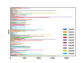
(a) Dirichlet 0.1

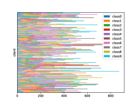
(b) Dirichlet 0.5

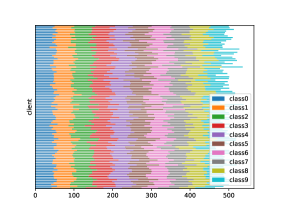
(c) Dirichlet 100

Figure 12: CIFAR10 data partitioning with Dirichlet distribution over 100 clients

This part presents further experiments that extend beyond the scope of the main text. Initially, we explored a scenario different from the extreme non-IID. Here, we conducted an experiment using a non-IID setting derived from the Dirichlet distribution, a common approach in numerous studies. We set the Dirichlet parameters to 0.1, 0.5, and 100, respectively, and distributed the data across 100 clients, as shown in Figure 12.

Dirichlet	Shifting	Uniform Quantization
		32+4bit		32+5bit		32+6bit		32+7bit		32+8bit
0.1	w/o Shift	N/A	-	45.6$\pm$6.79	+12.7	59.0$\pm$1.83	+2.5	62.5$\pm$1.35	+1.8	62.5$\pm$1.64	+2.2
	w/ Shift	N/A		58.3$\pm$2.70	$\sigma$:$\downarrow$60%	61.5$\pm$1.91	$\sigma$:$\uparrow$4%	64.3$\pm$1.35	$\sigma$:0%	64.7$\pm$1.58	$\sigma$:$\downarrow$4%
0.5	w/o Shift	N/A	-	43.2$\pm$28.63	+16.2	67.3$\pm$1.11	+2.8	68.9$\pm$0.60	+2.6	68.8$\pm$0.94	+3.3
	w/ Shift	N/A		59.4$\pm$2.27	$\sigma$:$\downarrow$91%	70.1$\pm$0.98	$\sigma$:$\downarrow$12%	71.5$\pm$0.82	$\sigma$:$\uparrow$37%	72.1$\pm$0.71	$\sigma$:$\downarrow$24%
100	w/o Shift	N/A	-	64.3$\pm$1.97	+3.1	71.1$\pm$0.46	+3.0	72.2$\pm$0.49	+3.3	72.1$\pm$0.12	+3.4
	w/ Shift	N/A		67.4$\pm$2.89	$\sigma$:$\uparrow$47%	74.1$\pm$0.40	$\sigma$:$\downarrow$13%	75.5$\pm$0.85	$\sigma$:$\uparrow$73%	75.5$\pm$0.57	$\sigma$:$\uparrow$375%
Dirichlet	Shifting	Non-uniform Quantization
		32+4bit		32+5bit		32+6bit		32+7bit		32+8bit
0.1	w/o Shift	53.3$\pm$1.17	0.0	57.3$\pm$1.86	+0.5	60.1$\pm$1.32	+1.4	61.5$\pm$1.46	+2.2	62.1$\pm$1.32	+2.0
	w/ Shift	53.3$\pm$2.31	$\sigma$:$\uparrow$97%	57.8$\pm$1.83	$\sigma$:$\downarrow$2%	61.5$\pm$1.36	$\sigma$:$\uparrow$3%	63.7$\pm$1.11	$\sigma$:$\downarrow$24%	64.1$\pm$1.24	$\sigma$:$\downarrow$6%
0.5	w/o Shift	63.3$\pm$1.06	+2.9	65.7$\pm$1.00	+0.9	66.9$\pm$1.16	+0.1	68.1$\pm$0.66	+3.3	66.1$\pm$0.96	+5.6
	w/ Shift	65.2$\pm$1.14	$\sigma$:$\uparrow$8%	66.6$\pm$0.97	$\sigma$:$\downarrow$3%	70.0$\pm$0.65	$\sigma$:$\downarrow$44%	71.4$\pm$0.43	$\sigma$:$\downarrow$35%	71.7$\pm$0.69	$\sigma$:$\downarrow$28%
100	w/o Shift	68.5$\pm$0.39	+2.1	70.2$\pm$0.26	+2.1	71.1$\pm$0.87	+3.1	71.7$\pm$0.29	+3.5	71.9$\pm$0.25	+3.6
	w/ Shift	70.6$\pm$0.58	$\sigma$:$\uparrow$49%	72.3$\pm$0.38	$\sigma$:$\uparrow$46%	74.2$\pm$0.26	$\sigma$:$\downarrow$70%	75.2$\pm$0.32	$\sigma$:$\uparrow$10%	75.5$\pm$0.51	$\sigma$:$\uparrow$104%

Table 3: Top-1 Accuracy Over 800 rounds for three independent running with different random seed

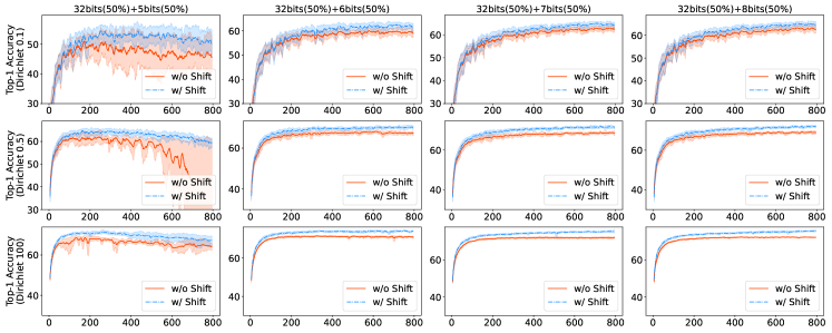
Figure 13: Top-1 accuracy throughout the training process under uniform quantization, as influenced by the Dirichlet distribution.

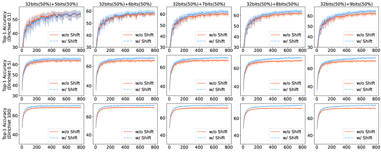
Figure 14: Top-1 accuracy throughout the training process under non-uniform quantization, as influenced by the Dirichlet distribution.

In this experiment, we employed a shifting technique exclusively with FedAvg. Performance was assessed for each Dirichlet distribution using two quantization techniques. Additionally, as in the main experiment, a combination approach was utilized, blending 50% of the 32-bit model and 50% of the quantized model from 4 to 8 bits. To refine the final performance results, we applied a Simple Moving Average (SMA) smoothing process with a window size of 10.

Figure 13 shows the performance result when uniform quantization is applied, and Figure 14 is the result of non-uniform quantization. We excluded the 4-bit quantization when we used uniform quantization for its unreliable behavior. The overall performance is summarized in Table 3. It is worth noting that with Dirichlet 100, the application of shifting generally led to an increase in most standard deviations. This phenomenon occurs as Dirichlet 100 is characterized by an IID (independently and identically distributed) data set format, which consistently demonstrates stable performance. The observed increase in standard deviation after shifting highlights this stability, as the deviation was already low prior to the shift.

C.2 CIFAR100 with Dirichlet Distribution

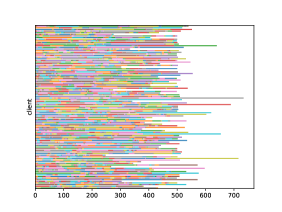
(a) Dirichlet 0.1

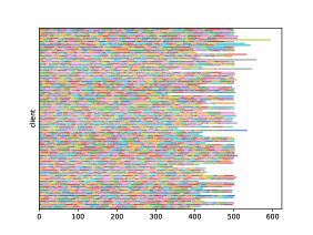
(b) Dirichlet 0.5

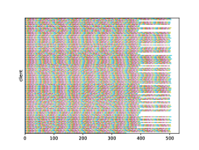
(c) Dirichlet 100

Figure 15: CIFAR100 data partitioning with Dirichlet distribution over 100 clients

Similarly, for the CIFAR100 dataset, three partitioning methods were configured using the Dirichlet distribution with parameters of 0.1, 0.5, and 100.

Dirichlet	32+32bit	Shifting	Uniform Quantization								Non-uniform Quantization
			5bit		6bit		7bit		8bit		4bit		5bit		6bit		7bit		8bit
0.1	52.40	w/o Shift	41.60	+6.80	50.37	+2.73	51.17	+2.71	51.78	+1.88	42.95	+3.80	48.99	+2.89	49.74	+2.61	50.67	+2.2	50.20	+2.83
		w/ Shift	48.40		53.10		53.88		53.66		46.75		51.88		52.35		52.89		52.03
0.5	54.00	w/o Shift	46.05	+5.91	52.56	+3.31	53.20	+2.89	53.54	+2.96	47.82	+4.33	50.78	+3.32	52.16	+3.48	53.62	+2.38	52.50	+4.08
		w/ Shift	51.96		55.87		56.09		56.50		52.15		54.10		55.64		56.00		56.58
100	55.18	w/o Shift	50.01	+3.52	53.16	+2.15	53.55	+1.92	53.05	+2.76	48.17	+4.68	50.63	+3.97	53.10	+3.30	53.72	+2.67	54.00	+2.80
		w/ Shift	53.53		55.31		55.47		55.81		52.85		54.60		56.40		56.39		56.80

Table 4: CIFAR100 dataset Top-3 Accuracy(%) after 400 rounds

With the CIFAR100 dataset, we employ the identical CNN model previously utilized for CIFAR10. Given the increased complexity of this dataset, we opt to evaluate Top-3 accuracy in this instance. FedShift demonstrates comparable improvements in performance on the CIFAR100 dataset as well, as shown in Table 4.

Appendix D Distributional Shift

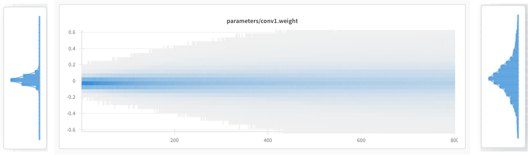
(a) 32+32bit

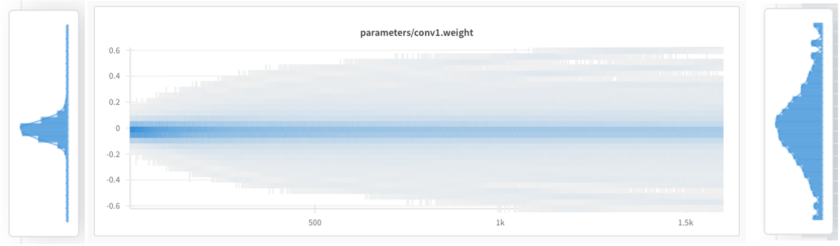
(b) 32+8bit

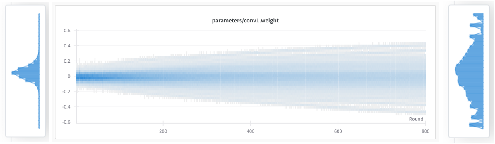
(c) 32+7bit

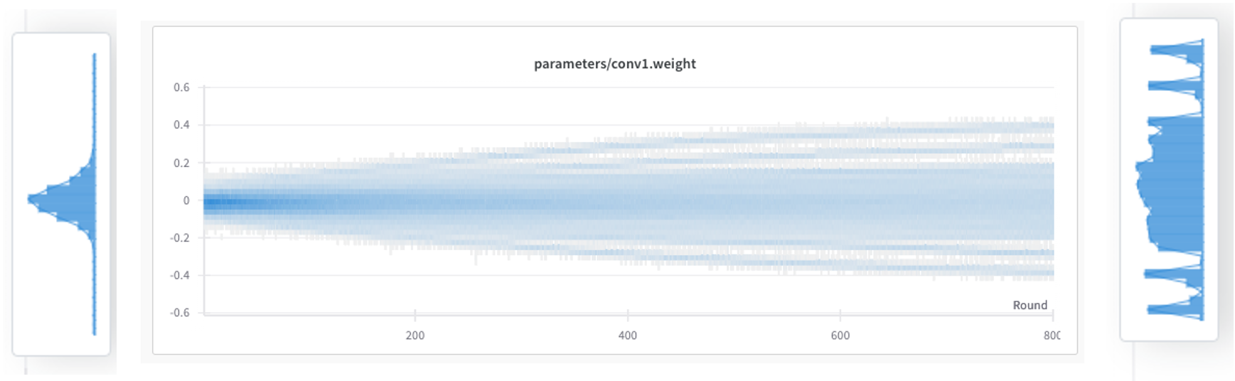
(d) 32+6bit

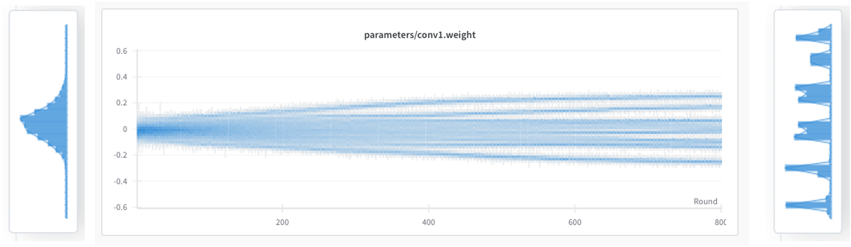
(e) 32+5bit

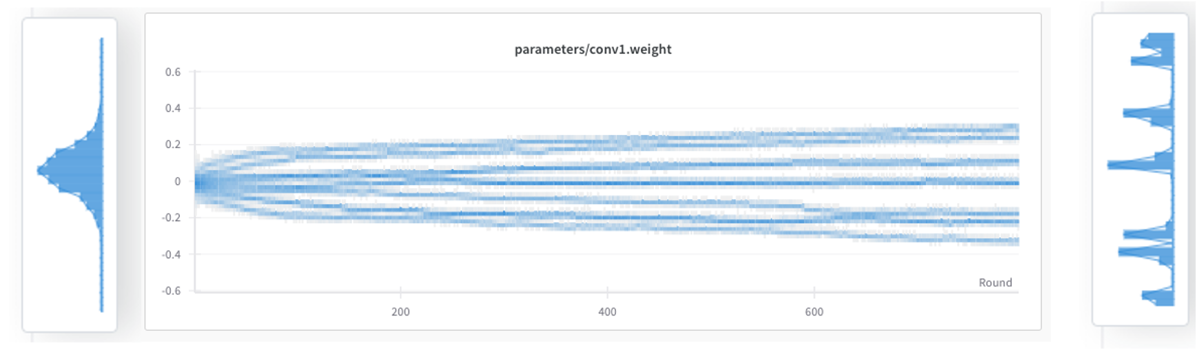
(f) 32+4bit

Figure 16: The impact of quantization at various bit levels on the evolution of weight distribution throughout a federated learning cycle. The histogram on the left depicts the initial distribution of weights, while the histogram on the right illustrates the distribution of weights after training. The chart in the middle tracks the progression across rounds, with denser lines indicating a higher concentration of values within that bin.

Figure 16 allows us to examine at what point the reduction in the number of quantization bits leads to a significant issue with the Distributional Shift. In the case of algorithms based on FedAvg using full-precision weights, we observe that although the width of the weight distribution changes from the initial to the final distribution, the bell-shaped curve following a normal distribution remains stable, as shown in Figure. This stability is evident up to 7-bit quantization. However, starting from 6 bits, we begin to see an increasing bias towards the extreme values, and by 4 bits, the final distribution barely resembles its original shape. Histograms of these weight distributions indicate that performance degradation does not occur with 7-bit quantization, and in some cases, it may even improve. This suggests that 128 ($2^{7}$) and 256 ($2^{8}$) bits are sufficient for representing the values that model weights should hold. Therefore, our primary focus should be on tackling the quantization at 4, 5, and 6 bits.

References

- Bonawitz et al. (2019) Bonawitz, K., Eichner, H., Grieskamp, W., Huba, D., Ingerman, A., Ivanov, V., Kiddon, C., Konečnỳ, J., Mazzocchi, S., McMahan, B., et al. Towards federated learning at scale: System design. Proceedings of Machine Learning and Systems, 1:374–388, 2019.
- Chen et al. (2021) Chen, S., Shen, C., Zhang, L., and Tang, Y. Dynamic aggregation for heterogeneous quantization in federated learning. IEEE Transactions on Wireless Communications, 20(10):6804–6819, 2021.
- Chen et al. (2020) Chen, Y., Ning, Y., Slawski, M., and Rangwala, H. Asynchronous online federated learning for edge devices with non-iid data. In 2020 IEEE International Conference on Big Data (Big Data), pp. 15–24. IEEE, 2020.
- Gholami et al. (2021) Gholami, A., Kim, S., Dong, Z., Yao, Z., Mahoney, M. W., and Keutzer, K. A survey of quantization methods for efficient neural network inference. arXiv preprint arXiv:2103.13630, 2021.
- Gong et al. (2014) Gong, Y., Liu, L., Yang, M., and Bourdev, L. Compressing deep convolutional networks using vector quantization. arXiv preprint arXiv:1412.6115, 2014.
- Guan et al. (2019) Guan, H., Malevich, A., Yang, J., Park, J., and Yuen, H. Post-training 4-bit quantization on embedding tables. arXiv preprint arXiv:1911.02079, 2019.
- Hamer et al. (2020) Hamer, J., Mohri, M., and Suresh, A. T. Fedboost: A communication-efficient algorithm for federated learning. In International Conference on Machine Learning, pp. 3973–3983. PMLR, 2020.
- Huang et al. (2017) Huang, L., Liu, X., Liu, Y., Lang, B., and Tao, D. Centered weight normalization in accelerating training of deep neural networks. In Proceedings of the IEEE International Conference on Computer Vision, pp. 2803–2811, 2017.
- Karimireddy et al. (2020) Karimireddy, S. P., Kale, S., Mohri, M., Reddi, S., Stich, S., and Suresh, A. T. Scaffold: Stochastic controlled averaging for federated learning. In International conference on machine learning, pp. 5132–5143. PMLR, 2020.
- Konečnỳ et al. (2016) Konečnỳ, J., McMahan, H. B., Ramage, D., and Richtárik, P. Federated optimization: Distributed machine learning for on-device intelligence. arXiv preprint arXiv:1610.02527, 2016.
- (11) Krizhevsky, A., Nair, V., and Hinton, G. Cifar-10 (canadian institute for advanced research). URL http://www.cs.toronto.edu/~kriz/cifar.html.
- Li et al. (2018) Li, T., Sahu, A. K., Zaheer, M., Sanjabi, M., Talwalkar, A., and Smith, V. Federated optimization in heterogeneous networks. arXiv preprint arXiv:1812.06127, 2018.
- Li et al. (2020) Li, T., Sahu, A. K., Zaheer, M., Sanjabi, M., Talwalkar, A., and Smith, V. Federated optimization in heterogeneous networks. Proceedings of Machine learning and systems, 2:429–450, 2020.
- Li et al. (2019) Li, X., Huang, K., Yang, W., Wang, S., and Zhang, Z. On the convergence of fedavg on non-iid data. In International Conference on Learning Representations, 2019.
- Luo et al. (2021) Luo, M., Chen, F., Hu, D., Zhang, Y., Liang, J., and Feng, J. No fear of heterogeneity: Classifier calibration for federated learning with non-iid data. Advances in Neural Information Processing Systems, 34:5972–5984, 2021.
- McMahan et al. (2017) McMahan, B., Moore, E., Ramage, D., Hampson, S., and y Arcas, B. A. Communication-efficient learning of deep networks from decentralized data. In Artificial intelligence and statistics, pp. 1273–1282. PMLR, 2017.
- Qiao et al. (2019) Qiao, S., Wang, H., Liu, C., Shen, W., and Yuille, A. Micro-batch training with batch-channel normalization and weight standardization. arXiv preprint arXiv:1903.10520, 2019.
- Rehman et al. (2023) Rehman, Y. A. U., Gao, Y., De Gusmão, P. P. B., Alibeigi, M., Shen, J., and Lane, N. D. L-dawa: Layer-wise divergence aware weight aggregation in federated self-supervised visual representation learning. In Proceedings of the IEEE/CVF International Conference on Computer Vision, pp. 16464–16473, 2023.
- Reisizadeh et al. (2020) Reisizadeh, A., Mokhtari, A., Hassani, H., Jadbabaie, A., and Pedarsani, R. Fedpaq: A communication-efficient federated learning method with periodic averaging and quantization. In International Conference on Artificial Intelligence and Statistics, pp. 2021–2031. PMLR, 2020.
- Salimans & Kingma (2016) Salimans, T. and Kingma, D. P. Weight normalization: A simple reparameterization to accelerate training of deep neural networks. Advances in neural information processing systems, 29, 2016.
- Shokri & Shmatikov (2015) Shokri, R. and Shmatikov, V. Privacy-preserving deep learning. In Proceedings of the 22nd ACM SIGSAC conference on computer and communications security, pp. 1310–1321, 2015.
- Stich (2018) Stich, S. U. Local sgd converges fast and communicates little. In International Conference on Learning Representations, 2018.
- Sun et al. (2019) Sun, J., Chen, T., Giannakis, G., and Yang, Z. Communication-efficient distributed learning via lazily aggregated quantized gradients. Advances in Neural Information Processing Systems, 32, 2019.
- Wang et al. (2020) Wang, J., Liu, Q., Liang, H., Joshi, G., and Poor, H. V. Tackling the objective inconsistency problem in heterogeneous federated optimization. Advances in neural information processing systems, 33:7611–7623, 2020.
- Wu & Flierl (2020) Wu, H. and Flierl, M. Vector quantization-based regularization for autoencoders. In Proceedings of the AAAI Conference on Artificial Intelligence, volume 34, pp. 6380–6387, 2020.
- Wu et al. (2016) Wu, J., Leng, C., Wang, Y., Hu, Q., and Cheng, J. Quantized convolutional neural networks for mobile devices. In Proceedings of the IEEE conference on computer vision and pattern recognition, pp. 4820–4828, 2016.
- Xie et al. (2019) Xie, C., Koyejo, S., and Gupta, I. Asynchronous federated optimization. arXiv preprint arXiv:1903.03934, 2019.
- Yoon et al. (2022) Yoon, J., Park, G., Jeong, W., and Hwang, S. J. Bitwidth heterogeneous federated learning with progressive weight dequantization. In International Conference on Machine Learning, pp. 25552–25565. PMLR, 2022.
- Yu et al. (2019) Yu, H., Yang, S., and Zhu, S. Parallel restarted sgd with faster convergence and less communication: Demystifying why model averaging works for deep learning. In Proceedings of the AAAI Conference on Artificial Intelligence, volume 33, pp. 5693–5700, 2019.
- Yuan et al. (2021) Yuan, Z., Guo, Z., Xu, Y., Ying, Y., and Yang, T. Federated deep auc maximization for hetergeneous data with a constant communication complexity. In International Conference on Machine Learning, pp. 12219–12229. PMLR, 2021.
- Zhang et al. (2012) Zhang, Y., Wainwright, M. J., and Duchi, J. C. Communication-efficient algorithms for statistical optimization. Advances in neural information processing systems, 25, 2012.
- Zhao et al. (2018) Zhao, Y., Li, M., Lai, L., Suda, N., Civin, D., and Chandra, V. Federated learning with non-iid data. arXiv preprint arXiv:1806.00582, 2018.