Multiclass Learning from Noisy Labels for
Non-decomposable Performance Measures
Mingyuan Zhang and Shivani Agarwal
University of Pennsylvania Philadelphia, PA 19104 {myz, ashivani}@seas.upenn.edu
Abstract
There has been much interest in recent years in learning good classifiers from data with noisy labels. Most work on learning from noisy labels has focused on standard loss-based performance measures. However, many machine learning problems require using non-decomposable performance measures which cannot be expressed as the expectation or sum of a loss on individual examples; these include for example the H-mean, Q-mean and G-mean in class imbalance settings, and the Micro in information retrieval. In this paper, we design algorithms to learn from noisy labels for two broad classes of multiclass non-decomposable performance measures, namely, monotonic convex and ratio-of-linear, which encompass all the above examples. Our work builds on the Frank-Wolfe and Bisection based methods of Narasimhan et al. (2015). In both cases, we develop noise-corrected versions of the algorithms under the widely studied family of class-conditional noise models. We provide regret (excess risk) bounds for our algorithms, establishing that even though they are trained on noisy data, they are Bayes consistent in the sense that their performance converges to the optimal performance w.r.t. the clean (non-noisy) distribution. Our experiments demonstrate the effectiveness of our algorithms in handling label noise.
1 INTRODUCTION
In many machine learning problems, the labels provided with the training data may be noisy. This can happen due to a variety of reasons, such as sensor measurement errors, human labeling errors, and data collection errors among others. Therefore, there has been much interest in recent years in learning good classifiers from data with noisy labels (Frénay and Verleysen,, 2014; Song et al.,, 2020; Han et al.,, 2020). Most work has focused on learning from noisy labels for standard loss-based performance measures; these include both the 0-1 loss and more general cost-sensitive losses, all of which are linear functions of the confusion matrix of a classifier. However, many machine learning problems require using non-decomposable performance measures which cannot be expressed as the expectation or sum of a loss on individual examples; these are general nonlinear functions of the confusion matrix, and include for example the H-mean, Q-mean and G-mean in class imbalance settings (Sun et al.,, 2006; Kennedy et al.,, 2009; Lawrence et al.,, 2012; Wang and Yao,, 2012), and the Micro in information retrieval (Manning et al.,, 2008; Kim et al.,, 2013). In this paper, we design algorithms to learn from noisy labels for two broad classes of multiclass non-decomposable performance measures, namely, monotonic convex and ratio-of-linear, which encompass all the above examples.
| Performance Measures | Standard (Non-noisy) Setting | Noisy Setting Under CCN Model |
|---|---|---|
| Loss-based (linear) | Many algorithms including surrogate risk minimization algorithms | Many noise-corrected algorithms (Natarajan et al.,, 2013; van Rooyen and Williamson,, 2017; Patrini et al.,, 2017; Zhang et al.,, 2021) |
| Monotonic convex | Frank-Wolfe based method | This work |
| (Narasimhan et al.,, 2015) | ||
| Ratio-of-linear | Bisection based method | This work |
| (Narasimhan et al.,, 2015) |
The main challenge in learning from noisy labels is to design algorithms which, given training data with noisy labels, can still learn accurate classifiers w.r.t. the clean/true distribution for a given target performance measure. For loss-based (linear) performance measures, previous works have designed Bayes consistent algorithms so that, when given sufficient noisy training data, their performance converges to the Bayes optimal performance w.r.t. the clean distribution (Natarajan et al.,, 2013; Scott et al.,, 2013; Scott,, 2015; Menon et al.,, 2015; Liu and Tao,, 2016; Patrini et al.,, 2016; Ghosh et al.,, 2017; van Rooyen and Williamson,, 2017; Patrini et al.,, 2017; Natarajan et al.,, 2017; Wang et al.,, 2018; Liu and Guo,, 2020; Zhang et al.,, 2021; Li et al.,, 2021). In this work, we provide similarly Bayes consistent noise-corrected algorithms for multiclass monotonic convex and ratio-of-linear performance measures, under the widely studied family of class-conditional noise (CCN) models. Our work builds on the Frank-Wolfe and Bisection based methods of Narasimhan et al., (2015), which were proposed for the standard (non-noisy) setting. Table 1 summarizes the position of our work relative to other consistent algorithms under the CCN model.
Our key contributions include the following:
-
•
Algorithms: We develop noise-corrected versions of the Frank-Wolfe and Bisection based algorithms for the families of monotonic convex and ratio-of-linear performance measures, respectively.
-
•
Theory: While the noise corrections we introduce are fairly intuitive, establishing the correctness of the resulting algorithms is not trivial. We provide regret (excess risk) bounds for our algorithms, establishing that even though they are trained on noisy data, they are Bayes consistent in the sense that their performance converges to the optimal performance w.r.t. the clean (non-noisy) distribution. The bounds quantify the effect of label noise on the sample complexity. We also provide extended regret bounds that quantify the effect of using an estimated noise matrix.
-
•
Empirical validations: We provide results of experiments on synthetic data verifying the sample complexity behavior of our algorithms, and also on real data comparing with previous baselines.
1.1 Related Work
Consistent algorithms for binary/multiclass classification for non-decomposable performance measures in the standard (non-noisy) setting. Most work in this category has focused on binary classification, for a variety of performance measures, including F-measure (Ye et al.,, 2012), the arithmetic mean of the true positive and true negative rates (AM) (Menon et al.,, 2013), ratio-of-linear performance measures (Koyejo et al.,, 2014; Bao and Sugiyama,, 2020), and monotonic performance measures (Narasimhan et al.,, 2014). Dembczynski et al., (2017) revisited consistency analysis in binary classification for non-decomposable performance measures for two distinct settings and notions of consistency (Population Utility and Expected Test Utility). For multiclass classification, Narasimhan et al., (2015) developed a general framework for designing provably consistent algorithms for monotonic convex and ratio-of-linear performance measures; an extended version of this work also studies such performance measures in constrained learning settings (Narasimhan et al.,, 2022). Parambath et al., (2014); Koyejo et al., (2015); Natarajan et al., (2016) also designed algorithms for some multiclass non-decomposable performance measures. All of these works designed algorithms for standard (non-noisy) settings. Our methods, which build on Narasimhan et al., (2015), are designed to correct for noisy labels for monotonic convex and ratio-of-linear performance measures, with provable consistency guarantees.
Consistent algorithms for binary/multiclass learning from noisy labels for the 0-1 or cost-sensitive losses. For the CCN model in binary classification, many consistent algorithms have been proposed and analyzed (Natarajan et al.,, 2013; Scott et al.,, 2013; Menon et al.,, 2015; Liu and Tao,, 2016; Patrini et al.,, 2016; Liu and Guo,, 2020). Scott et al., (2013); Scott, (2015); Menon et al., (2015); Liu and Tao, (2016) also proposed consistent estimators for noise rates when they are not known (additional assumptions required). Scott et al., (2013); Menon et al., (2015) studied the more general mutually contaminated distributions (MCD) noise model for binary classification, and proposed consistent algorithms. Natarajan et al., (2017) studied cost-sensitive loss functions. Progress has also been made in instance-dependent and label-dependent noise (ILN) model (Menon et al.,, 2018; Cheng et al.,, 2020). For the multiclass CCN model, Ghosh et al., (2017); van Rooyen and Williamson, (2017); Patrini et al., (2017); Wang et al., (2018); Zhang et al., (2021); Li et al., (2021) proposed consistent algorithms. All the methods above are designed to handle noisy labels for loss-based performance measures; our work, on the other hand, focuses on non-decomposable performance measures.
Consistent algorithms for binary learning from noisy labels for non-decomposable performance measures. The method in Scott et al., (2013) focused on the minmax error. Menon et al., (2015) focused mostly on the balanced error (BER) and area under the ROC curve (AUC) metrics. Both studied the MCD model (which includes CCN model). All these results are for binary classification. Our proposed algorithms, under the CCN model, are designed for monotonic convex and ratio-of-linear performance measures in both binary and multiclass classification settings.
Performance measures in multi-label classification and structured prediction. There is also a line of work studying performance measures (e.g., Hamming loss and -measure) in multi-label classification and structured prediction problems (Zhang and Zhou,, 2014; Li et al.,, 2016; Wang et al.,, 2017; Zhang et al.,, 2020), but those are distinct from (albeit related to) non-decomposable performance measures in multiclass classification settings as considered in this work.
1.2 Organization and Notation
Organization. After preliminaries and background in Section 2, we describe our noise-corrected algorithms for two broad classes of non-decomposable performance measures (monotonic convex and ratio-of-linear) in Section 3 and Section 4, respectively. Section 5 provides consistency guarantees for our algorithms in the form of regret bounds. Section 6 summarizes our experiments. Section 7 concludes the paper. All proofs can be found in Appendix A.
Notation. For an integer , we denote by the set of integers , and by the probability simplex . For a vector , we denote by the -norm of , and by the -th entry of . For a matrix , we denote by the induced matrix -norm of , and by the -th column vector of . We use to denote the -th entry of . In addition, we use for the matrix analogue of the vector -norm.111Note that and in Narasimhan et al., (2015) are and in our notations. We choose to follow conventional definitions of the matrix norm in the literature instead. For matrices , we define . The indicator function is .
2 PRELIMINARIES AND BACKGROUND
Multiclass learning from noisy labels. Let be the instance space, and be the label space. Without loss of generality, we assume . There is an unknown distribution over . In a standard multiclass learning problem, the learner is given labeled examples drawn from . However, when learning from noisy labels, the learner is only given noisy examples , where is the corresponding noisy label for . The learner’s goal is to learn a classifier using the noisy training sample, so that its performance is good w.r.t. the clean distribution.
We consider the class-conditional noise (CCN) model (Natarajan et al.,, 2013; van Rooyen and Williamson,, 2017; Patrini et al.,, 2017), in which a label is switched by the noise process to with probability that only depends on (and not on ). This noise can be fully described by a column stochastic matrix.
Definition 1 (Class-conditional noise matrix).
The class-conditional noise matrix, , is column stochastic with entries .
We assume is invertible. In practice, often needs to be estimated; several methods have been developed to estimate from the noisy sample (Xia et al.,, 2019; Yao et al.,, 2020; Li et al.,, 2021). Our algorithms and theoretical guarantees work with both known and estimated .
We can then view the noisy training examples as being drawn i.i.d. from a noisy distribution on . Specifically, to generate , an example is firstly drawn according to , and then is switched to according to noise matrix .
Non-decomposable performance measure. To measure the performance of a classifier , or more generally, a randomized classifier (which for a given instance , predicts a label according to the probability specified by ), we consider performance measures that are general functions of confusion matrices.
Definition 2 (Confusion matrix).
The confusion matrix of a (possibly randomized) classifier w.r.t. a distribution , denoted by , has entries , where denotes a random draw of label from distribution when is randomized.
Definition 3 (Performance measure).
For any function , define the -performance measure of w.r.t. as
We adopt the convention that lower values of correspond to better performance.
The following shows this formulation of performance measure includes the common loss-based performance measures (e.g., the 0-1 loss and cost-sensitive losses).
Example 1 (-performance measures).
Consider a multiclass loss matrix , where is the loss incurred for predicting when the true class is . Then for a deterministic classifier ,
In fact, loss-based performance measures are linear functions of confusion matrices. For nonlinear , -performance measures are non-decomposable, i.e., they cannot be expressed as the expected loss on a new example drawn from . Common examples of such non-decomposable performance measures include Micro in information retrieval (Manning et al.,, 2008; Kim et al.,, 2013), H-mean, Q-mean and G-mean in class imbalance settings (Kennedy et al.,, 2009; Lawrence et al.,, 2012; Sun et al.,, 2006; Wang and Yao,, 2012), and others.222See Table 1 of Narasimhan et al., (2015).
Learning goal. Given a noisy training sample drawn according to the noisy distribution , the goal of the learner is to learn a (randomized) classifier that performs well w.r.t. for a pre-specified -performance measure. In particular, we want the performance of to converge (in probability) to Bayes optimal -performance as the training sample size increases. Below we define Bayes optimal -performance as the optimal value over feasible confusion matrices.
Definition 4 (Feasible confusion matrices).
Feasible confusion matrices w.r.t. are all possible confusion matrices achieved by randomized classifiers. Define as the set of feasible confusion matrices w.r.t. as
We note that is a convex set (Narasimhan et al., (2015)).
Definition 5 (Bayes optimal -performance).
For any function , define the Bayes optimal -performance w.r.t. as
In the following sections, we focus on two broad classes of non-decomposable performance measures, namely monotonic convex and ratio-of-linear. The former includes H-mean, Q-mean and G-mean, and the latter includes Micro .
3 MONOTONIC CONVEX PERFORMANCE MEASURES
Our work develops noise-corrected versions of the algorithms of Narasimhan et al., (2015). Below, we describe two key operations on which the algorithms in Narasimhan et al., (2015) are built; we then describe our noise-corrected algorithm for monotonic convex performance measures. We will show how we use the noise matrix to correct the two operations to learn from noisy labels. We note that the noise correction operations work with estimated as well. We start with the definition and some examples of monotonic convex performance measures.
Definition 6 (Monotonic convex performance measures).
A performance measure is monotonic convex if for any confusion matrix , is convex in , and monotonically (strictly) decreasing in and non-decreasing in for .
Example 2 (H-mean, Q-mean and G-mean, all in loss forms).
H-mean: , Q-mean: , and G-mean: .
Next, we sketch the idea behind the algorithms in Narasimhan et al., (2015), and show how to introduce noise corrections to learn from noisy labels. We first define the class probability function.
Definition 7 (Class probability function, class probability for short).
For , the class probability function is defined as for . Similarly for , we define as for .
Idea behind algorithms in the standard (non-noisy) setting (Narasimhan et al.,, 2015). The algorithmic framework optimizes the non-decomposable performance measure of interest through an iterative approach (based on the Frank-Wolfe method for the monotonic convex case, and based on the bisection method for the ratio-of-linear case; details later), which in each iteration , approximates the target performance measure by a linear loss-based performance measure . Each iteration involves two key operations: OP1 and OP2. OP1 involves finding an optimal classifier for the current linear approximation . This is done by using a class probability estimator (CPE) learned from the (clean) training sample, and then defining classifier as . OP2 involves estimating , the confusion matrix of w.r.t. , by , the empirical confusion matrix of w.r.t. sample defined below:
| (1) |
Note that converges to as increases. (More specifically, to facilitate consistency analysis, the iterative algorithms split the training sample into and . is used to learn a CPE model , and in each iterative step , is used to calculate via OP2.)
Noise-corrected algorithm for monotonic convex performance measures. We are now ready to describe our approach. In learning from noisy labels, the algorithm only sees noisy sample . Our approach is to introduce noise corrections to both OP1 and OP2, so the modified algorithm can still output a good classifier w.r.t. the clean distribution .
Noise-corrected OP1. Recall OP1 involves finding an optimal classifier for a loss-based performance measure w.r.t. . To do so with a noisy sample, we propose to find an optimal classifier for a noise-corrected loss-based performance measure w.r.t. according to the following proposition.
Proposition 8.
Let . Then any Bayes optimal classifier for -performance w.r.t. is also Bayes optimal for -performance w.r.t. .
This idea has also been used in multiclass noisy label settings with -performance (van Rooyen and Williamson,, 2017; Zhang et al.,, 2021).
Noise-corrected OP2. Recall OP2 is to estimate . We need to do so with noisy sample . We first observe a relation between clean confusion matrix and noisy confusion matrix under noise matrix .
Proposition 9.
For a given classifier , the relation between clean confusion matrix and noisy confusion matrix under CCN matrix is .
So we propose to estimate by . In Section 5, we will show this gives a consistent estimate, i.e., converges to as the size of increases.
We can now incorporate the noise-corrected OP1 and OP2 into the iterative algorithm based on Frank-Wolfe method (Frank and Wolfe,, 1956; Narasimhan et al.,, 2015). The noise-corrected algorithm is summarized in Algorithm 1. This algorithm applies to monotonic convex performance measures , such as H-mean, Q-mean and G-mean. It seeks to solve with the noisy sample . Note that the form in Line 7 comes from the form of Bayes optimal classifier for monotonic convex performance measures in the standard (non-noisy) setting (Theorem 13 of Narasimhan et al., (2015)). Specifically, Algorithm 1 maintains implicitly via . At each step , it applies noise-corrected OP1 and OP2 to construct a loss matrix and solve a linear minimization problem, and to compute an empirical confusion matrix. The final randomized classifier is a convex combination of all the classifiers . In Section 5, we will formally prove the noise-corrected algorithm is consistent.
4 RATIO-OF-LINEAR PERFORMANCE MEASURES
We now move to the next family of non-decomposable performance measures, namely ratio-of-linear performance measures. We start with the definition and an example. Then we will show how to use the noise-corrected OP1 and OP2 described in Section 3 to build an algorithm to learn from noisy labels for ratio-of-linear performance measures. We will also provide another view of the algorithm from the perspective of correcting the performance measure .
Definition 10 (Ratio-of-linear performance measures).
A performance measure is ratio-of-linear if there are such that for any confusion matrix , and .
Example 3 (Micro in loss form).
Micro : .
Noise-corrected algorithm for ratio-of-linear performance measures. The iterative algorithm based on Bisection method (Lemaréchal,, 2006; Narasimhan et al.,, 2015) follows broadly a similar idea as described in Section 3, so we can use the same noise-corrected OP1 and OP2 to modify the algorithm. The noise-corrected algorithm is summarized in Algorithm 2. This algorithm applies to ratio-of-linear performance measures , such as Micro . It uses a binary search approach to find the minimum value of . Note that the form in Line 7 comes from the form of Bayes optimal classifier for ratio-of–linear performance measures in the standard (non-noisy) setting (Theorem 11 of Narasimhan et al., (2015)). Again, Algorithm 2 maintains implicitly via . At each step , it applies noise-corrected OP1 and OP2 to construct a loss matrix and solve a linear minimization problem, and to compute an empirical confusion matrix. The final classifier is deterministic. In Section 5, we will formally prove the noise-corrected algorithm is consistent.
We also offer another view of Algorithm 2 from the perspective of correcting . In particular, we show that one can construct a noise-corrected performance measure , which is also ratio-of-linear. Then one can simply optimize using a noisy sample to learn a classifier , and the learned will also be optimal for the original performance measure w.r.t. the clean distribution .
Theorem 11 (Form of Bayes optimal classifier for ratio-of-linear by correcting ).
Consider ratio-of-linear performance measure with . Define noise-corrected performance measure by . Then with for all . Moreover, any Bayes optimal classifier for -performance w.r.t. is also Bayes optimal for -performance w.r.t. .
Therefore, one can view Algorithm 2 as finding the Bayes optimal classifier for w.r.t. the noisy distribution , which in turn is also Bayes optimal for w.r.t. the clean distribution . This view is reminiscent of the Unbiased Estimator approach in van Rooyen and Williamson, (2017) and Backward method in Patrini et al., (2017), in which one optimizes noise-corrected surrogate losses using a noisy sample to learn classifiers that are optimal w.r.t. the clean distribution.
5 CONSISTENCY AND REGRET BOUNDS
In this section, we derive quantitative regret bounds for our noise-corrected algorithms. Our results show that when the CPE learner used in the algorithms is consistent (i.e., it converges to the noisy class probabilities), then the noise-corrected algorithms are consistent, i.e., they can output classifiers whose -performance converges to the Bayes optimal -performance w.r.t. as the size of the noisy training sample increases. In addition, we provide regret bounds for our algorithms when estimated is used instead of . To start, we formally define what it means for a learning algorithm to be -consistent when learning from noisy labels.
Definition 12 (-regret).
For any function and classifier , define -regret of w.r.t. as the difference between -performance of and the Bayes optimal -performance: .
Definition 13 (-consistent algorithm when learning from noisy labels).
For , we say a multiclass algorithm , which given a noisy sample of size outputs a (randomized) classifier , is consistent for w.r.t. if for all :
In Appendix A, we provide guarantees for the noise-corrected OP1 and OP2 (Lemma 18 and Lemma 19). They are used in deriving the following regret bounds.
Theorem 14 (-regret bound for Algorithm 1).
Let be monotonic convex over , and -Lipschitz and -smooth w.r.t. norm.333A function is -smooth if its gradient is -Lipschitz. Noisy sample is drawn randomly from . Let be the CPE model learned from as in Algorithm 1. Then for , with probability at least (over ), we have
where is a distribution-independent constant.
Theorem 15 (-regret bound for Algorithm 2).
Let for with for some . Noisy sample is drawn randomly from . Let be the CPE model learned from as in Algorithm 2. Then for , with probability at least (over ), we have
where and is a distribution-independent constant.
In particular, using a strongly/strictly proper composite surrogate loss (e.g., multiclass logistic regression loss/cross entropy loss with softmax function) over a universal function class (with suitable regularization) to learn a CPE model ensures a consistent noisy class probability estimation, i.e., as the sample size increases (Agarwal,, 2014; Williamson et al.,, 2016; Zhang et al.,, 2021). This leads to the convergence of the regret to zero as . Also, as the amount of label noise (captured by ) increases, the bounds get larger; one might therefore need a larger noisy sample size to achieve the same level of -regret w.r.t. . Our synthetic experiments also confirm this sample complexity behavior.
Regret bounds with estimated . When noise matrix is not known, one may need to use estimated . Several methods have been developed to estimate from the noisy sample (Xia et al.,, 2019; Yao et al.,, 2020; Li et al.,, 2021). Below, we provide regret bounds for our noise-corrected algorithms when estimated is used. They involve an additional factor that quantifies the quality of the estimated .
6 EXPERIMENTS
We conducted two sets of experiments. In the first set of experiments, we generated synthetic data and tested the sample complexity behavior of our algorithms. In the second set of experiments, we used real data and compared our algorithms with other algorithms. Our code is available at https://github.com/moshimowang/noisy-labels-non-decomposable.
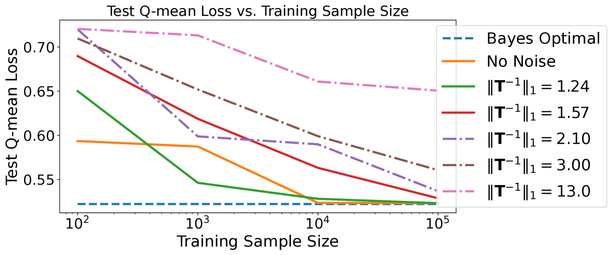
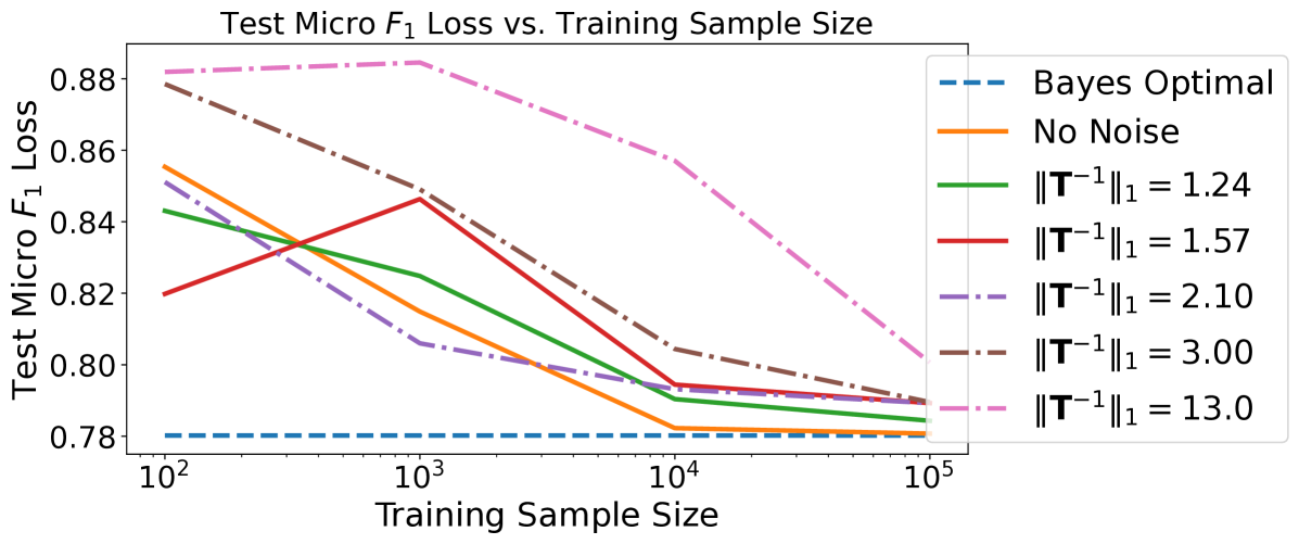
Sample complexity behavior. We tested the sample complexity behavior of our algorithm on synthetic data generated from a known distribution (see Appendix B for the data generating process). We generated noise matrices by choosing a noise level and setting diagonal entries of to and off-diagonal entries of to . We tested the sample complexity behavior of our algorithms for a variety of noise matrices with increasing values of noise level . The corresponding values of were also increasing. The non-decomposable performance measures were Q-mean and Micro . We applied Algorithm 1 for Q-mean with and Algorithm 2 for Micro with . In both algorithms, the CPE learner was implemented by minimizing the multiclass logistic regression loss (aka. cross entropy loss with softmax function) over linear functions. We ran the algorithms on noisy training samples with increasing sizes (, , ), and measured the performance on a clean test set of examples. The results are shown in Figure 1. The top plot shows results for Q-mean. The bottom plot shows results for Micro . We see that, as suggested by our regret bounds, as increases (i.e., more noise), the sample size required to achieve a given level of performance generally increases.
| Data sets | Algorithms | ||||
|---|---|---|---|---|---|
| vehicle | FW | 0.255 (0.005) | 0.267 (0.011) | 0.309 (0.007) | 0.373 (0.010) |
| NCFW | 0.254 (0.007) | 0.266 (0.015) | 0.307 (0.008) | 0.338 (0.013) | |
| NCLR-Backward | 0.482 (0.024) | 0.573 (0.020) | 0.512 (0.033) | 0.508 (0.021) | |
| NCLR-Forward | 0.512 (0.035) | 0.563 (0.021) | 0.570 (0.011) | 0.563 (0.029) | |
| NCLR-Plug-in | 0.515 (0.016) | 0.567 (0.010) | 0.517 (0.028) | 0.540 (0.015) | |
| pageblocks | FW | 0.380 (0.041) | 0.286 (0.011) | 0.633 (0.097) | 0.627 (0.066) |
| NCFW | 0.269 (0.017) | 0.253 (0.006) | 0.535 (0.019) | 0.528 (0.034) | |
| NCLR-Backward | 1.000 (0.000) | 1.000 (0.000) | 1.000 (0.000) | 1.000 (0.000) | |
| NCLR-Forward | 1.000 (0.000) | 1.000 (0.000) | 1.000 (0.000) | 1.000 (0.000) | |
| NCLR-Plug-in | 1.000 (0.000) | 1.000 (0.000) | 1.000 (0.000) | 0.926 (0.066) | |
| satimage | FW | 0.188 (0.005) | 0.224 (0.005) | 0.247 (0.006) | 0.340 (0.006) |
| NCFW | 0.186 (0.005) | 0.222 (0.006) | 0.230 (0.005) | 0.300 (0.005) | |
| NCLR-Backward | 0.556 (0.023) | 0.630 (0.026) | 0.685 (0.043) | 0.960 (0.012) | |
| NCLR-Forward | 0.542 (0.020) | 0.522 (0.011) | 0.612 (0.030) | 0.877 (0.017) | |
| NCLR-Plug-in | 0.679 (0.049) | 0.793 (0.023) | 0.854 (0.031) | 0.902 (0.021) | |
| covtype | FW | 0.569 (0.001) | 0.591 (0.001) | 0.771 (0.010) | 0.741 (0.009) |
| NCFW | 0.525 (0.001) | 0.569 (0.001) | 0.606 (0.002) | 0.706 (0.004) | |
| NCLR-Backward | 1.000 (0.000) | 1.000 (0.000) | 1.000 (0.000) | 1.000 (0.000) | |
| NCLR-Forward | 0.995 (0.001) | 0.987 (0.002) | 0.980 (0.002) | 0.963 (0.005) | |
| NCLR-Plug-in | 1.000 (0.000) | 1.000 (0.000) | 1.000 (0.000) | 1.000 (0.000) | |
| abalone | FW | 0.806 (0.014) | 0.799 (0.006) | 0.812 (0.006) | 0.801 (0.010) |
| NCFW | 0.797 (0.008) | 0.795 (0.006) | 0.804 (0.008) | 0.814 (0.010) | |
| NCLR-Backward | 1.000 (0.000) | 1.000 (0.000) | 1.000 (0.000) | 1.000 (0.000) | |
| NCLR-Forward | 1.000 (0.000) | 1.000 (0.000) | 1.000 (0.000) | 1.000 (0.000) | |
| NCLR-Plug-in | 1.000 (0.000) | 1.000 (0.000) | 1.000 (0.000) | 1.000 (0.000) |
| Data sets | Algorithms | ||||
|---|---|---|---|---|---|
| vehicle | BS | 0.268 (0.007) | 0.307 (0.006) | 0.323 (0.013) | 0.388 (0.012) |
| NCBS | 0.264 (0.008) | 0.299 (0.006) | 0.314 (0.011) | 0.346 (0.009) | |
| NCLR-Backward | 0.435 (0.020) | 0.524 (0.006) | 0.508 (0.027) | 0.494 (0.028) | |
| NCLR-Forward | 0.470 (0.031) | 0.483 (0.020) | 0.548 (0.016) | 0.553 (0.030) | |
| NCLR-Plug-in | 0.494 (0.022) | 0.488 (0.023) | 0.491 (0.025) | 0.521 (0.015) | |
| pageblocks | BS | 0.231 (0.009) | 0.323 (0.011) | 0.862 (0.005) | 0.899 (0.006) |
| NCBS | 0.251 (0.008) | 0.261 (0.010) | 0.320 (0.006) | 0.404 (0.020) | |
| NCLR-Backward | 0.515 (0.050) | 0.457 (0.055) | 0.756 (0.079) | 0.510 (0.048) | |
| NCLR-Forward | 0.823 (0.083) | 0.880 (0.048) | 0.743 (0.113) | 0.832 (0.093) | |
| NCLR-Plug-in | 0.609 (0.096) | 0.595 (0.107) | 0.568 (0.051) | 0.795 (0.045) | |
| satimage | BS | 0.219 (0.004) | 0.224 (0.002) | 0.242 (0.002) | 0.313 (0.003) |
| NCBS | 0.219 (0.004) | 0.220 (0.003) | 0.236 (0.002) | 0.292 (0.002) | |
| NCLR-Backward | 0.215 (0.004) | 0.222 (0.003) | 0.227 (0.004) | 0.231 (0.003) | |
| NCLR-Forward | 0.217 (0.003) | 0.214 (0.002) | 0.213 (0.003) | 0.221 (0.003) | |
| NCLR-Plug-in | 0.234 (0.002) | 0.236 (0.003) | 0.255 (0.002) | 0.300 (0.003) | |
| covtype | BS | 0.361 (0.000) | 0.355 (0.000) | 0.362 (0.000) | 0.362 (0.000) |
| NCBS | 0.361 (0.000) | 0.352 (0.000) | 0.362 (0.000) | 0.362 (0.000) | |
| NCLR-Backward | 0.384 (0.000) | 0.385 (0.000) | 0.388 (0.000) | 0.390 (0.001) | |
| NCLR-Forward | 0.384 (0.000) | 0.380 (0.000) | 0.381 (0.001) | 0.382 (0.001) | |
| NCLR-Plug-in | 0.398 (0.000) | 0.396 (0.001) | 0.397 (0.000) | 0.397 (0.000) | |
| abalone | BS | 0.731 (0.007) | 0.746 (0.005) | 0.746 (0.003) | 0.750 (0.002) |
| NCBS | 0.729 (0.007) | 0.743 (0.005) | 0.740 (0.003) | 0.754 (0.001) | |
| NCLR-Backward | 0.787 (0.005) | 0.789 (0.007) | 0.797 (0.010) | 0.793 (0.011) | |
| NCLR-Forward | 0.774 (0.007) | 0.806 (0.004) | 0.783 (0.003) | 0.794 (0.009) | |
| NCLR-Plug-in | 0.789 (0.005) | 0.789 (0.009) | 0.803 (0.007) | 0.799 (0.010) |
Comparison with other algorithms. We conducted experiments on several real data sets taken from UCI Machine Learning Repository (Dua and Graff,, 2017). Details of the data sets are in Appendix C. We compared our noise-corrected algorithms (NCFW and NCBS) with the baseline Frank-Wolfe (FW) and Bisection (BS) based methods of Narasimhan et al., (2015, 2022) that were designed for the standard (non-noisy) learning setting, as well as various previously proposed noise-corrected versions of multiclass logistic regression (NCLR-Backward (van Rooyen and Williamson,, 2017; Patrini et al.,, 2017), NCLR-Forward (Patrini et al.,, 2017), and NCLR-Plug-in (Zhang et al.,, 2021)). We used the authors’ implementations for FW and BS.444https://github.com/shivtavker/constrained-classification. To ensure a fair comparison, we also implemented our algorithms in the same framework. Different variants of NCLR were implemented based on Patrini et al., (2017).555https://github.com/giorgiop/loss-correction. A linear function class is used in all algorithms; see Appendix C for more details.
To generate noise matrices , we chose a noise level , set diagonal entries of to , and set off-diagonal entries uniformly at random from so that each column of sums to . This makes sure that on average, percent of clean labels were flipped to other labels, i.e., . Therefore, higher value of means a higher noise level. We generated 4 noise matrices with according to this process. Training labels were flipped randomly according to the prescribed noise matrix .
We ran FW and NCFW for iterative steps, and ran BS and NCBS for iterative steps. Performance of the learned model was then measured on a clean test set. The results are summarized in Table 2 (for H-mean loss) and Table 3 (for Micro loss), shown as the mean (with standard error of the mean in parentheses) over 5 random train-test splits. Higher is a high noise level. For each data set and each noise level, the best performance is shown in bold font. The results for G-mean loss and Q-mean loss can be found in Appendix C. As expected, in most cases, NCFW and NCBS outperform FW and BS, respectively, and they outperform variants of noise-corrected multiclass logistic regression as well.
7 CONCLUSION
We have provided the first known noise-corrected algorithms, NCFW and NCBS, for multiclass monotonic convex and ratio-of-linear performance measures under general class-conditional noise models. We have also provided regret bounds for our algorithms showing that they are consistent w.r.t. the clean data distribution, and quantifying the effect of noise on their sample complexity. Our experiments have demonstrated the effectiveness of our algorithms in handling label noise. For settings where the noise matrix may be unknown, approaches for estimating have been proposed in the literature. These can be combined with our algorithms where needed, and we have also provided regret bounds for our algorithms when estimated is used.
Acknowledgements
The authors thank Harikrishna Narasimhan, Harish G. Ramaswamy, and Shiv Kumar Tavker for helpful discussions and for sharing the code of their work. Thanks to the anonymous reviewers for several helpful comments and pointers. This material is based upon work supported in part by the US National Science Foundation (NSF) under Grant Nos. 1934876. Any opinions, findings, and conclusions or recommendations expressed in this material are those of the authors and do not necessarily reflect the views of the National Science Foundation.
References
- Abadi et al., (2015) Abadi, M., Agarwal, A., Barham, P., Brevdo, E., Chen, Z., Citro, C., Corrado, G. S., Davis, A., Dean, J., Devin, M., Ghemawat, S., Goodfellow, I., Harp, A., Irving, G., Isard, M., Jia, Y., Jozefowicz, R., Kaiser, L., Kudlur, M., Levenberg, J., Mané, D., Monga, R., Moore, S., Murray, D., Olah, C., Schuster, M., Shlens, J., Steiner, B., Sutskever, I., Talwar, K., Tucker, P., Vanhoucke, V., Vasudevan, V., Viégas, F., Vinyals, O., Warden, P., Wattenberg, M., Wicke, M., Yu, Y., and Zheng, X. (2015). TensorFlow: Large-scale machine learning on heterogeneous systems. Software available from tensorflow.org.
- Agarwal, (2014) Agarwal, S. (2014). Surrogate regret bounds for bipartite ranking via strongly proper losses. Journal of Machine Learning Research, 15:1653–1674.
- Bao and Sugiyama, (2020) Bao, H. and Sugiyama, M. (2020). Calibrated surrogate maximization of linear-fractional utility in binary classification. In The 23rd International Conference on Artificial Intelligence and Statistics, AISTATS 2020, volume 108 of Proceedings of Machine Learning Research, pages 2337–2347. PMLR.
- Cheng et al., (2020) Cheng, J., Liu, T., Ramamohanarao, K., and Tao, D. (2020). Learning with bounded instance and label-dependent label noise. In Proceedings of the 37th International Conference on Machine Learning, ICML 2020, volume 119 of Proceedings of Machine Learning Research, pages 1789–1799. PMLR.
- Dembczynski et al., (2017) Dembczynski, K., Kotlowski, W., Koyejo, O., and Natarajan, N. (2017). Consistency analysis for binary classification revisited. In Proceedings of the 34th International Conference on Machine Learning, ICML 2017, volume 70 of Proceedings of Machine Learning Research, pages 961–969. PMLR.
- Dua and Graff, (2017) Dua, D. and Graff, C. (2017). UCI machine learning repository.
- Frank and Wolfe, (1956) Frank, M. and Wolfe, P. (1956). An algorithm for quadratic programming. Naval Research Logistics Quarterly, 3(1-2):95–110.
- Frénay and Verleysen, (2014) Frénay, B. and Verleysen, M. (2014). Classification in the presence of label noise: A survey. IEEE Trans. Neural Networks Learn. Syst., 25(5):845–869.
- Ghosh et al., (2017) Ghosh, A., Kumar, H., and Sastry, P. S. (2017). Robust loss functions under label noise for deep neural networks. In Proceedings of the Thirty-First AAAI Conference on Artificial Intelligence, 2017, pages 1919–1925. AAAI Press.
- Han et al., (2020) Han, B., Yao, Q., Liu, T., Niu, G., Tsang, I. W., Kwok, J. T., and Sugiyama, M. (2020). A survey of label-noise representation learning: Past, present and future. CoRR, abs/2011.04406.
- Kennedy et al., (2009) Kennedy, K., Namee, B. M., and Delany, S. J. (2009). Learning without default: A study of one-class classification and the low-default portfolio problem. In Artificial Intelligence and Cognitive Science - 20th Irish Conference, AICS 2009, Revised Selected Papers, volume 6206 of Lecture Notes in Computer Science, pages 174–187. Springer.
- Kim et al., (2013) Kim, J., Wang, Y., and Yamamoto, Y. (2013). The genia event extraction shared task, 2013 edition - overview. In Proceedings of the BioNLP Shared Task 2013 Workshop, pages 8–15. Association for Computational Linguistics.
- Koyejo et al., (2014) Koyejo, O., Natarajan, N., Ravikumar, P., and Dhillon, I. S. (2014). Consistent binary classification with generalized performance metrics. In Advances in Neural Information Processing Systems 27: Annual Conference on Neural Information Processing Systems 2014, pages 2744–2752.
- Koyejo et al., (2015) Koyejo, O., Natarajan, N., Ravikumar, P., and Dhillon, I. S. (2015). Consistent multilabel classification. In Advances in Neural Information Processing Systems 28: Annual Conference on Neural Information Processing Systems 2015, pages 3321–3329.
- Lawrence et al., (2012) Lawrence, S., Burns, I., Back, A. D., Tsoi, A. C., and Giles, C. L. (2012). Neural network classification and prior class probabilities. In Neural Networks: Tricks of the Trade - Second Edition, volume 7700 of Lecture Notes in Computer Science, pages 295–309. Springer.
- Lemaréchal, (2006) Lemaréchal, C. (2006). S. boyd, l. vandenberghe, convex optimization, cambridge university press, 2004 hardback, ISBN 0 521 83378 7. Eur. J. Oper. Res., 170(1):326–327.
- Li et al., (2016) Li, J., Asif, K., Wang, H., Ziebart, B. D., and Berger-Wolf, T. Y. (2016). Adversarial sequence tagging. In Proceedings of the Twenty-Fifth International Joint Conference on Artificial Intelligence, IJCAI 2016, pages 1690–1696. IJCAI/AAAI Press.
- Li et al., (2021) Li, X., Liu, T., Han, B., Niu, G., and Sugiyama, M. (2021). Provably end-to-end label-noise learning without anchor points. In Proceedings of the 38th International Conference on Machine Learning, ICML 2021, volume 139 of Proceedings of Machine Learning Research, pages 6403–6413. PMLR.
- Liu and Tao, (2016) Liu, T. and Tao, D. (2016). Classification with noisy labels by importance reweighting. IEEE Trans. Pattern Anal. Mach. Intell., 38(3):447–461.
- Liu and Guo, (2020) Liu, Y. and Guo, H. (2020). Peer loss functions: Learning from noisy labels without knowing noise rates. In Proceedings of the 37th International Conference on Machine Learning, ICML 2020, volume 119, pages 6226–6236. PMLR.
- Manning et al., (2008) Manning, C. D., Raghavan, P., and Schütze, H. (2008). Introduction to information retrieval. Cambridge University Press.
- Menon et al., (2013) Menon, A. K., Narasimhan, H., Agarwal, S., and Chawla, S. (2013). On the statistical consistency of algorithms for binary classification under class imbalance. In Proceedings of the 30th International Conference on Machine Learning, ICML 2013, volume 28 of JMLR Workshop and Conference Proceedings, pages 603–611. JMLR.org.
- Menon et al., (2018) Menon, A. K., van Rooyen, B., and Natarajan, N. (2018). Learning from binary labels with instance-dependent noise. Mach. Learn., 107(8-10):1561–1595.
- Menon et al., (2015) Menon, A. K., van Rooyen, B., Ong, C. S., and Williamson, B. (2015). Learning from corrupted binary labels via class-probability estimation. In Proceedings of the 32nd International Conference on Machine Learning, ICML 2015, volume 37, pages 125–134. JMLR.org.
- Narasimhan et al., (2015) Narasimhan, H., Ramaswamy, H. G., Saha, A., and Agarwal, S. (2015). Consistent multiclass algorithms for complex performance measures. In Proceedings of the 32nd International Conference on Machine Learning, ICML 2015, volume 37 of JMLR Workshop and Conference Proceedings, pages 2398–2407. JMLR.org.
- Narasimhan et al., (2022) Narasimhan, H., Ramaswamy, H. G., Tavker, S. K., Khurana, D., Netrapalli, P., and Agarwal, S. (2022). Consistent multiclass algorithms for complex metrics and constraints. CoRR, abs/2210.09695.
- Narasimhan et al., (2014) Narasimhan, H., Vaish, R., and Agarwal, S. (2014). On the statistical consistency of plug-in classifiers for non-decomposable performance measures. In Advances in Neural Information Processing Systems 27: Annual Conference on Neural Information Processing Systems 2014, pages 1493–1501.
- Natarajan et al., (2013) Natarajan, N., Dhillon, I. S., Ravikumar, P., and Tewari, A. (2013). Learning with noisy labels. In Advances in Neural Information Processing Systems 26: 27th Annual Conference on Neural Information Processing Systems 2013, pages 1196–1204.
- Natarajan et al., (2017) Natarajan, N., Dhillon, I. S., Ravikumar, P., and Tewari, A. (2017). Cost-sensitive learning with noisy labels. J. Mach. Learn. Res., 18:155:1–155:33.
- Natarajan et al., (2016) Natarajan, N., Koyejo, O., Ravikumar, P., and Dhillon, I. S. (2016). Optimal classification with multivariate losses. In Proceedings of the 33nd International Conference on Machine Learning, ICML 2016, volume 48 of JMLR Workshop and Conference Proceedings, pages 1530–1538. JMLR.org.
- Parambath et al., (2014) Parambath, S. P., Usunier, N., and Grandvalet, Y. (2014). Optimizing f-measures by cost-sensitive classification. In Advances in Neural Information Processing Systems 27: Annual Conference on Neural Information Processing Systems 2014, pages 2123–2131.
- Patrini et al., (2016) Patrini, G., Nielsen, F., Nock, R., and Carioni, M. (2016). Loss factorization, weakly supervised learning and label noise robustness. In Proceedings of the 33nd International Conference on Machine Learning, ICML 2016, volume 48 of JMLR Workshop and Conference Proceedings, pages 708–717. JMLR.org.
- Patrini et al., (2017) Patrini, G., Rozza, A., Menon, A. K., Nock, R., and Qu, L. (2017). Making deep neural networks robust to label noise: A loss correction approach. In 2017 IEEE Conference on Computer Vision and Pattern Recognition, CVPR 2017, pages 2233–2241. IEEE Computer Society.
- Pedregosa et al., (2011) Pedregosa, F., Varoquaux, G., Gramfort, A., Michel, V., Thirion, B., Grisel, O., Blondel, M., Prettenhofer, P., Weiss, R., Dubourg, V., Vanderplas, J., Passos, A., Cournapeau, D., Brucher, M., Perrot, M., and Duchesnay, E. (2011). Scikit-learn: Machine learning in Python. Journal of Machine Learning Research, 12:2825–2830.
- Scott, (2015) Scott, C. (2015). A rate of convergence for mixture proportion estimation, with application to learning from noisy labels. In Proceedings of the Eighteenth International Conference on Artificial Intelligence and Statistics, AISTATS 2015, volume 38. JMLR.org.
- Scott et al., (2013) Scott, C., Blanchard, G., and Handy, G. (2013). Classification with asymmetric label noise: Consistency and maximal denoising. In COLT 2013 - The 26th Annual Conference on Learning Theory, volume 30, pages 489–511. JMLR.org.
- Song et al., (2020) Song, H., Kim, M., Park, D., and Lee, J. (2020). Learning from noisy labels with deep neural networks: A survey. CoRR, abs/2007.08199.
- Sun et al., (2006) Sun, Y., Kamel, M. S., and Wang, Y. (2006). Boosting for learning multiple classes with imbalanced class distribution. In Proceedings of the 6th IEEE International Conference on Data Mining (ICDM 2006), pages 592–602. IEEE Computer Society.
- van Rooyen and Williamson, (2017) van Rooyen, B. and Williamson, R. C. (2017). A theory of learning with corrupted labels. J. Mach. Learn. Res., 18:228:1–228:50.
- Wang et al., (2017) Wang, H., Rezaei, A., and Ziebart, B. D. (2017). Adversarial structured prediction for multivariate measures. CoRR, abs/1712.07374.
- Wang et al., (2018) Wang, R., Liu, T., and Tao, D. (2018). Multiclass learning with partially corrupted labels. IEEE Trans. Neural Networks Learn. Syst., 29(6):2568–2580.
- Wang and Yao, (2012) Wang, S. and Yao, X. (2012). Multiclass imbalance problems: Analysis and potential solutions. IEEE Trans. Syst. Man Cybern. Part B, 42(4):1119–1130.
- Williamson et al., (2016) Williamson, R. C., Vernet, E., and Reid, M. D. (2016). Composite multiclass losses. J. Mach. Learn. Res., 17:223:1–223:52.
- Xia et al., (2019) Xia, X., Liu, T., Wang, N., Han, B., Gong, C., Niu, G., and Sugiyama, M. (2019). Are anchor points really indispensable in label-noise learning? In Advances in Neural Information Processing Systems 32: Annual Conference on Neural Information Processing Systems 2019, NeurIPS 2019, pages 6835–6846.
- Yao et al., (2020) Yao, Y., Liu, T., Han, B., Gong, M., Deng, J., Niu, G., and Sugiyama, M. (2020). Dual T: reducing estimation error for transition matrix in label-noise learning. In Advances in Neural Information Processing Systems 33: Annual Conference on Neural Information Processing Systems 2020, NeurIPS 2020.
- Ye et al., (2012) Ye, N., Chai, K. M. A., Lee, W. S., and Chieu, H. L. (2012). Optimizing f-measure: A tale of two approaches. In Proceedings of the 29th International Conference on Machine Learning, ICML 2012. icml.cc / Omnipress.
- Zhang et al., (2021) Zhang, M., Lee, J., and Agarwal, S. (2021). Learning from noisy labels with no change to the training process. In Proceedings of the 38th International Conference on Machine Learning, volume 139, pages 12468–12478. PMLR.
- Zhang et al., (2020) Zhang, M., Ramaswamy, H. G., and Agarwal, S. (2020). Convex calibrated surrogates for the multi-label f-measure. In Proceedings of the 37th International Conference on Machine Learning, volume 119, pages 11246–11255. PMLR.
- Zhang and Zhou, (2014) Zhang, M. and Zhou, Z. (2014). A review on multi-label learning algorithms. IEEE Trans. Knowl. Data Eng., 26(8):1819–1837.
Checklist
-
1.
For all models and algorithms presented, check if you include:
-
(a)
A clear description of the mathematical setting, assumptions, algorithm, and/or model. [Yes]
-
(b)
An analysis of the properties and complexity (time, space, sample size) of any algorithm. [Yes]
-
(c)
(Optional) Anonymized source code, with specification of all dependencies, including external libraries. [Yes]
-
(a)
-
2.
For any theoretical claim, check if you include:
-
(a)
Statements of the full set of assumptions of all theoretical results. [Yes]
-
(b)
Complete proofs of all theoretical results. [Yes]
-
(c)
Clear explanations of any assumptions. [Yes]
-
(a)
-
3.
For all figures and tables that present empirical results, check if you include:
-
(a)
The code, data, and instructions needed to reproduce the main experimental results (either in the supplemental material or as a URL). [Yes]
-
(b)
All the training details (e.g., data splits, hyperparameters, how they were chosen). [Yes]
-
(c)
A clear definition of the specific measure or statistics and error bars (e.g., with respect to the random seed after running experiments multiple times). [Yes]
-
(d)
A description of the computing infrastructure used. (e.g., type of GPUs, internal cluster, or cloud provider). [Yes; see Appendix]
-
(a)
-
4.
If you are using existing assets (e.g., code, data, models) or curating/releasing new assets, check if you include:
-
(a)
Citations of the creator If your work uses existing assets. [Yes]
-
(b)
The license information of the assets, if applicable. [Not Applicable]
-
(c)
New assets either in the supplemental material or as a URL, if applicable. [Not Applicable]
-
(d)
Information about consent from data providers/curators. [Not Applicable]
-
(e)
Discussion of sensible content if applicable, e.g., personally identifiable information or offensive content. [Not Applicable]
-
(a)
-
5.
If you used crowdsourcing or conducted research with human subjects, check if you include:
-
(a)
The full text of instructions given to participants and screenshots. [Not Applicable]
-
(b)
Descriptions of potential participant risks, with links to Institutional Review Board (IRB) approvals if applicable. [Not Applicable]
-
(c)
The estimated hourly wage paid to participants and the total amount spent on participant compensation. [Not Applicable]
-
(a)
Multiclass Learning from Noisy Labels for
Non-decomposable Performance Measures
Supplementary Materials
Appendix A Proofs
A.1 Proofs for Section 3
Proof of Proposition 8.
Proof.
Let be a Bayes optimal classifier for -performance w.r.t. . So
where we have used properties of the adjoint in the second “=”.
Note that for any , we have
So is also Bayes optimal for -performance w.r.t. , i.e., . ∎
Proof of Proposition 9.
Proof.
∎
A.2 Proofs for Section 4
Proof of Theorem 11.
Proof.
By property of adjoint, we have
For all , there exists such that . So,
This shows for all .
Let be a Bayes optimal classifier for -performance w.r.t. (the existence of such a classifier is guaranteed by Theorem 11 of Narasimhan et al., (2015)). So,
For all ,
This shows is also Bayes optimal for -performance w.r.t. . ∎
A.3 Proofs for Section 5
Lemma 18 (Guarantee for noise-corrected OP1).
Let be the CPE model learned from noisy sample . Then
Proof of Lemma 18.
Proof.
∎
Lemma 19 (Guarantee for noise-corrected OP2).
For , let be the empirical confusion matrix w.r.t. noisy sample (computed similarly as in Eq. (1)). Then
Proof of Lemma 19.
Proof.
∎
Notes for Lemma 18 and Lemma 19: In Lemma 18, might be viewed as an estimate for . If the CPE model used is consistent (i.e., as the sample size increases), then this estimation is consistent as well. Similarly, in Lemma 19, might be viewed as an estimate for . Because the confusion matrix estimator in Eq. (1) is consistent (i.e., as the sample size increases) as shown in Lemma 15 of Narasimhan et al., (2015), this estimation is also consistent. might be viewed as a constant capturing the overall amount of label noise.
Notes for our proof of Theorem 14: Our proof of Theorem 14 uses Lemma 14, Lemma 15 and Theorem 16 in Narasimhan et al., (2015), along with their proofs. We include a proposition below that summarizes the key aspects of Lemma 14, Lemma 15 and Theorem 16 in Narasimhan et al., (2015) that we make use of (with slight modification in order for it to be consistent with our notations).
Proposition 20 (-regret bound of Frank-Wolfe based algorithm in the non-noisy setting; Theorem 16 in Narasimhan et al., (2015)).
Let be monotonic convex over , and -Lipschitz and -smooth w.r.t. norm. Let clean sample be drawn randomly from . Let be the CPE model learned from as in the Frank-Wolfe based algorithm, and be the classifier returned after iterations. Let . Then with probability (over ),
where is a distribution-independent constant, and . The second ‘’ was obtained by Lemma 15 of Narasimhan et al., (2015) and .
Proof of Theorem 14.
Proof.
In Algorithm 1, we only have noisy sample that is split into and . We implicitly estimate by , where is a CPE model learned from . Lemma 18 shows an additional factor of as a price paid to learn from a noisy sample instead of a clean one. For a classifier , we estimate by , where is the empirical confusion matrix learned from . Lemma 19 shows an additional factor of as a cost to learn from a noisy sample instead of a clean one. Note that for . Chaining this reasoning with Proposition 20 establishes the claim. ∎
Notes for our proof of Theorem 15: Our proof of Theorem 15 uses Lemma 14, Lemma 15 and Theorem 17 in Narasimhan et al., (2015), along with their proofs. We include a proposition below that summarizes the key aspects of Lemma 14, Lemma 15 and Theorem 17 in Narasimhan et al., (2015) that we make use of (with slight modification in order for it to be consistent with our notations).
Proposition 21 (-regret bound for bisection based algorithm in the non-noisy setting; Theorem 17 in Narasimhan et al., (2015)).
Let for with for some . Let clean sample be drawn randomly from . Let be the CPE model learned from as in the bisection based algorithm, and be the classifier returned after iterations. Let . Then with probability (over ),
where , is a distribution-independent constant, and . The second ‘’ was obtained by Lemma 15 of Narasimhan et al., (2015) and .
Proof of Theorem 15.
Proof.
In Algorithm 2, we only have noisy sample that is split into and . We implicitly estimate by , where is a CPE model learned from . Lemma 18 shows an additional factor of as a price paid to learn from a noisy sample instead of a clean one. For a classifier , we estimate by , where is the empirical confusion matrix learned from . Lemma 19 shows an additional factor of as a cost to learn from a noisy sample instead of a clean one. Note that for . Chaining this reasoning with Proposition 21 establishes the claim. ∎
Lemma 22 (Guarantee for noise-corrected OP1 with estimated ).
Let be the CPE model learned from noisy sample . Let be an estimate of . Then
Proof of Lemma 22.
Proof.
∎
Lemma 23 (Guarantee for noise-corrected OP2 with estimated ).
For , let be the empirical confusion matrix w.r.t. noisy sample (computed similarly as in Eq. (1)). Let be an estimate of . Then
Proof of Lemma 23.
Proof.
∎
Proof of Theorem 16.
Proof.
Proof of Theorem 17.
Appendix B Synthetic Data: Additional Details
Data generating process. Specifically, we constructed a 3-class problem over a 2-dimensional instance space as follows. Instances were generated according to a fixed Gaussian mixture distribution. The class probability function was for some fixed weight vectors and bias terms . Given an instance , a clean label was drawn randomly according to . Then was flipped to a noisy label according to the probabilities in the -th column of , where is a prescribed column stochastic noise matrix.
Appendix C Real Data: Additional Details and Experiments
For NCFW, NCBS, FW, and BS, the linear model CPE learner was implemented using scikit-learn (Pedregosa et al.,, 2011). The different variants of NCLR, implemented in TensorFlow (Abadi et al.,, 2015), also used a linear function class. In all cases, regularization parameters were chosen by cross-validation.
Table 4 gives details of the real data sets used in Section 6. Table 5 and Table 6 give results for G-mean loss and Q-mean loss, respectively.
| Data set | # instances | # classes | # features |
|---|---|---|---|
| vehicle | 846 | 4 | 18 |
| pageblocks | 5,473 | 5 | 10 |
| satimage | 6,435 | 6 | 36 |
| covtype | 581,012 | 7 | 14 |
| abalone | 4,177 | 12 | 8 |
| Data sets | Algorithms | ||||
|---|---|---|---|---|---|
| vehicle | FW | 0.230 (0.007) | 0.249 (0.011) | 0.287 (0.009) | 0.349 (0.011) |
| NCFW | 0.231 (0.008) | 0.247 (0.012) | 0.289 (0.009) | 0.312 (0.012) | |
| NCLR-Backward | 0.432 (0.017) | 0.519 (0.013) | 0.488 (0.034) | 0.469 (0.025) | |
| NCLR-Forward | 0.463 (0.030) | 0.496 (0.015) | 0.523 (0.012) | 0.524 (0.025) | |
| NCLR-Plug-in | 0.477 (0.016) | 0.503 (0.012) | 0.486 (0.021) | 0.502 (0.013) | |
| pageblocks | FW | 0.331 (0.026) | 0.225 (0.009) | 0.552 (0.081) | 0.563 (0.046) |
| NCFW | 0.236 (0.040) | 0.167 (0.010) | 0.503 (0.125) | 0.382 (0.018) | |
| NCLR-Backward | 1.000 (0.000) | 1.000 (0.000) | 1.000 (0.000) | 1.000 (0.000) | |
| NCLR-Forward | 1.000 (0.000) | 1.000 (0.000) | 1.000 (0.000) | 1.000 (0.000) | |
| NCLR-Plug-in | 1.000 (0.000) | 1.000 (0.000) | 1.000 (0.000) | 0.898 (0.091) | |
| satimage | FW | 0.181 (0.004) | 0.214 (0.004) | 0.225 (0.005) | 0.310 (0.005) |
| NCFW | 0.180 (0.005) | 0.213 (0.004) | 0.212 (0.005) | 0.272 (0.005) | |
| NCLR-Backward | 0.368 (0.010) | 0.400 (0.013) | 0.428 (0.020) | 0.684 (0.072) | |
| NCLR-Forward | 0.362 (0.009) | 0.351 (0.005) | 0.385 (0.011) | 0.524 (0.014) | |
| NCLR-Plug-in | 0.439 (0.023) | 0.486 (0.012) | 0.550 (0.023) | 0.638 (0.019) | |
| covtype | FW | 0.570 (0.001) | 0.577 (0.001) | 0.685 (0.004) | 0.690 (0.005) |
| NCFW | 0.515 (0.001) | 0.516 (0.001) | 0.546 (0.001) | 0.612 (0.004) | |
| NCLR-Backward | 1.000 (0.000) | 1.000 (0.000) | 1.000 (0.000) | 1.000 (0.000) | |
| NCLR-Forward | 0.908 (0.021) | 0.875 (0.003) | 0.869 (0.002) | 0.847 (0.004) | |
| NCLR-Plug-in | 1.000 (0.000) | 1.000 (0.000) | 1.000 (0.000) | 1.000 (0.000) | |
| abalone | FW | 0.779 (0.008) | 0.775 (0.002) | 0.786 (0.005) | 0.778 (0.005) |
| NCFW | 0.776 (0.007) | 0.766 (0.001) | 0.781 (0.007) | 0.784 (0.005) | |
| NCLR-Backward | 1.000 (0.000) | 1.000 (0.000) | 1.000 (0.000) | 1.000 (0.000) | |
| NCLR-Forward | 1.000 (0.000) | 1.000 (0.000) | 1.000 (0.000) | 1.000 (0.000) | |
| NCLR-Plug-in | 1.000 (0.000) | 1.000 (0.000) | 1.000 (0.000) | 1.000 (0.000) |
| Data sets | Algorithms | ||||
|---|---|---|---|---|---|
| vehicle | FW | 0.268 (0.008) | 0.287 (0.012) | 0.313 (0.009) | 0.367 (0.006) |
| NCFW | 0.276 (0.005) | 0.293 (0.009) | 0.310 (0.010) | 0.334 (0.011) | |
| NCLR-Backward | 0.449 (0.011) | 0.518 (0.010) | 0.495 (0.031) | 0.480 (0.022) | |
| NCLR-Forward | 0.473 (0.023) | 0.501 (0.011) | 0.527 (0.011) | 0.527 (0.023) | |
| NCLR-Plug-in | 0.486 (0.016) | 0.504 (0.011) | 0.489 (0.021) | 0.507 (0.013) | |
| pageblocks | FW | 0.352 (0.023) | 0.276 (0.005) | 0.499 (0.021) | 0.547 (0.030) |
| NCFW | 0.267 (0.016) | 0.201 (0.004) | 0.426 (0.032) | 0.466 (0.036) | |
| NCLR-Backward | 0.684 (0.022) | 0.683 (0.036) | 0.776 (0.033) | 0.715 (0.031) | |
| NCLR-Forward | 0.850 (0.024) | 0.800 (0.039) | 0.812 (0.042) | 0.861 (0.019) | |
| NCLR-Plug-in | 0.695 (0.039) | 0.641 (0.045) | 0.681 (0.026) | 0.677 (0.055) | |
| satimage | FW | 0.197 (0.005) | 0.228 (0.006) | 0.246 (0.006) | 0.323 (0.006) |
| NCFW | 0.199 (0.006) | 0.232 (0.005) | 0.252 (0.007) | 0.312 (0.005) | |
| NCLR-Backward | 0.390 (0.004) | 0.403 (0.007) | 0.412 (0.005) | 0.443 (0.002) | |
| NCLR-Forward | 0.386 (0.005) | 0.380 (0.003) | 0.393 (0.004) | 0.425 (0.001) | |
| NCLR-Plug-in | 0.425 (0.004) | 0.435 (0.003) | 0.465 (0.003) | 0.528 (0.006) | |
| covtype | FW | 0.567 (0.001) | 0.570 (0.001) | 0.639 (0.001) | 0.653 (0.001) |
| NCFW | 0.546 (0.001) | 0.544 (0.001) | 0.624 (0.000) | 0.623 (0.001) | |
| NCLR-Backward | 0.736 (0.001) | 0.744 (0.001) | 0.752 (0.001) | 0.768 (0.001) | |
| NCLR-Forward | 0.729 (0.001) | 0.734 (0.001) | 0.732 (0.001) | 0.732 (0.001) | |
| NCLR-Plug-in | 0.799 (0.000) | 0.802 (0.000) | 0.813 (0.000) | 0.813 (0.000) | |
| abalone | FW | 0.754 (0.005) | 0.762 (0.003) | 0.763 (0.005) | 0.767 (0.003) |
| NCFW | 0.753 (0.005) | 0.760 (0.003) | 0.770 (0.006) | 0.775 (0.004) | |
| NCLR-Backward | 0.910 (0.004) | 0.919 (0.004) | 0.917 (0.006) | 0.910 (0.010) | |
| NCLR-Forward | 0.892 (0.008) | 0.921 (0.004) | 0.902 (0.004) | 0.910 (0.006) | |
| NCLR-Plug-in | 0.907 (0.006) | 0.915 (0.007) | 0.911 (0.005) | 0.908 (0.006) |
Appendix D Computing Resource
We ran all experiments on a desktop with one AMD Threadripper 3960X CPU and one Nvidia GeForce RTX 3090 GPU.