Weakly Convex Regularisers for Inverse Problems:
Convergence of Critical Points and Primal-Dual Optimisation

Abstract

Variational regularisation is the primary method for solving inverse problems, and recently there has been considerable work leveraging deeply learned regularisation for enhanced performance. However, few results exist addressing the convergence of such regularisation, particularly within the context of critical points as opposed to global minima. In this paper, we present a generalised formulation of convergent regularisation in terms of critical points, and show that this is achieved by a class of weakly convex regularisers. We prove convergence of the primal-dual hybrid gradient method for the associated variational problem, and, given a Kurdyka–Łojasiewicz condition, an $\mathcal{O}(\log{k}/k)$ ergodic convergence rate. Finally, applying this theory to learned regularisation, we prove universal approximation for input weakly convex neural networks (IWCNN), and show empirically that IWCNNs can lead to improved performance of learned adversarial regularisers for computed tomography (CT) reconstruction.

Key words: Image reconstruction, inverse problems, learned regularisation, weak convexity, deep learning, computed tomography, convergent regularisation, primal-dual optimisation.

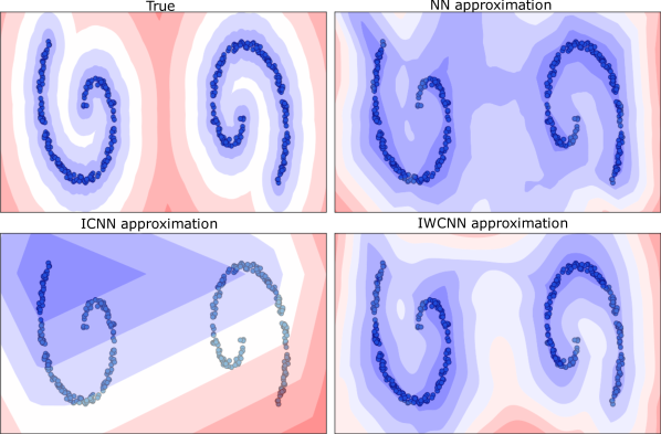
Figure 1: Contour plots comparing the distance function to a data manifold (top-left) with learned regularisers for denoising this data, via convex (bottom-left), standard (top-right), and weakly convex (bottom-right) adversarial regularisation. The convex regulariser lacks an interpretation as a distance function, whilst the weakly convex regulariser, introduced in this work, retains this feature and shows improved generalisation.

1 Introduction

In an inverse problem, one seeks to recover an unknown parameter (e.g., an image) that has undergone some, typically lossy and noisy, transformation (e.g., during measurement). Such problems arise frequently in science, e.g. in medical imaging such as in MRI, CT, and PET, and also beyond science, e.g. in art restoration [Natterer, 2001, Scherzer et al., 2009, Calatroni et al., 2018].

Mathematically, one seeks to estimate an unknown parameter $x^{*}\in\operatorname{\mathcal{X}}$ from a transformed and noisy measurement

$$y^{\delta}=\mathcal{A}x^{*}+\eta\in\operatorname{\mathcal{Y}},$$ (1.1)

see [Engl et al., 1996]. Here $\operatorname{\mathcal{X}}$ and $\operatorname{\mathcal{Y}}$ are Banach spaces; $\mathcal{A}:\operatorname{\mathcal{X}}\rightarrow\operatorname{\mathcal{Y}}$ is the forward model, assumed to be linear and bounded, e.g. representing imaging physics; and $\eta\in\operatorname{\mathcal{Y}}$, with $\left\|\eta\right\|_{\operatorname{\mathcal{Y}}}\leqslant\delta$, describes measurement noise. However, Equation 1.1 is usually ill-posed, i.e. $x\in\operatorname{\mathcal{X}}$ with $\operatorname{\mathcal{A}}x=y^{\delta}$ may not exist, be unique, or be continuous in $y^{\delta}$.

An influential technique to overcome this ill-posedness has been the variational approach pioneered by [Tikhonov, 1963] and [Phillips, 1962]:

$$x^{\alpha}(y^{\delta})\in\operatorname*{argmin}_{x\in\operatorname{\mathcal{X}}}\left\{\alpha\mathcal{R}(x)+\mathcal{D}\left(\operatorname{\mathcal{A}}x,y^{\delta}\right)=:\mathcal{J}_{\alpha,y^{\delta}}(x)\right\}.$$ (1.2)

Here: $\mathcal{R}:\operatorname{\mathcal{X}}\rightarrow{\mathbb{R}}$ is the regulariser, which aims to incorporate prior knowledge about $x^{*}$ and penalise $x$ if it is not ‘realistic’; $\mathcal{D}:\operatorname{\mathcal{Y}}\times\operatorname{\mathcal{Y}}\rightarrow{\mathbb{R}}$ is the data-fidelity term, which quantifies the distance between $y^{\delta}$ and $\operatorname{\mathcal{A}}x$ and comes from the distribution of the noise $\eta$; and $\alpha>0$ balances the relative importance of the two terms. A regularisation method is well-defined if $x^{\alpha}(y^{\delta})$ is stable with respect to data perturbations and converges to a solution of the operator equation.

A good choice of regulariser $\mathcal{R}$ is important for achieving accurate results. Traditional regularisation was knowledge-driven: the regulariser was a hand-crafted functional designed to encourage the reconstruction $x$ to have structures known to be realistic. Over the past decades, a whole zoo of such regularisers have been proposed, see e.g. [Rudin et al., 1992, Bredies et al., 2010, Gilboa and Osher, 2009, Mallat, 2009, Kutyniok and Labate, 2012, Lassas et al., 2009, Davoli et al., 2023] and see [Benning and Burger, 2018] for a detailed overview. However, there is a limit to the complexity of patterns that can be described by a hand-crafted functional.

Seeking to overcome this limitation, there has been considerable recent interest in data-driven approaches to inverse problems, see [Arridge et al., 2019] for a detailed overview. A key data-driven technique is to learn the regulariser from data. Such methods include: dictionary learning (see [Chen and Needell, 2016] for an overview), plug-and-play priors [Venkatakrishnan et al., 2013], regularisation by denoising [Romano et al., 2017], deep image priors [Lempitsky et al., 2018, Dittmer et al., 2019], generative regularisation (see [Dimakis, 2022] for an overview), and adversarial regularisation [Lunz et al., 2018]. These methods typically outperform knowledge-driven regularisation in practice.

1.1 Motivation and contributions

A key challenge in the data-driven paradigm is proving guarantees about the behaviour of the learned models. In [Mukherjee et al., 2023] the role of convexity, via the input convex neural network architecture [Amos et al., 2017], was emphasised as a method for achieving such guarantees, e.g. in the case of the adversarial convex regulariser (ACR) [Mukherjee et al., 2021]. But convexity is quite a restrictive condition, and the ACR sacrifices the adversarial regulariser’s interpretability as a distance function to the data manifold (see Figure 1), contributing to worse performance. It has been observed in the literature that non-convex regularisers often have better performance [Mohimani et al., 2009, Roth and Black, 2009, Pieper and Petrosyan, 2022]. Of particular interest is recent work on ‘optimal’ regularisation [Alberti et al., 2021, Leong et al., 2023], as such optimal regularisers are typically non-convex. This non-convexity returns us to a setting in which provable guarantees are challenging to achieve. However, the optimal regulariser of [Alberti et al., 2021] is often weakly convex, and weak convexity offers a more structured setting for reasoning about the non-convex case, see e.g. [Pinilla et al., 2022].

Optimisation methods in the context of weak convexity can be split into either subgradient or proximal based methods; see [Drusvyatskiy and Davis, 2020] for an introductory review. Subgradient methods admit strong iteration complexity guarantees [Davis et al., 2018, Davis and Drusvyatskiy, 2018, Goujon et al., 2024]. However, the convergence settings for these methods are somewhat narrow. Proximal methods admit significantly improved complexity bounds, as well as objective convergence rates [Hurault et al., 2022]. These rates can be further improved through prox-linearisation [Drusvyatskiy and Paquette, 2019, Davis and Drusvyatskiy, 2022] or adaptive steps [Böhm and Wright, 2021].

Of particular interest for optimising Equation 1.2 is the proximal primal-dual method, first analysed for convex functions in [Chambolle and Pock, 2011]. The first guarantees for primal-dual in the context of weak convexity were shown in [Möllenhoff et al., 2015], which assumed the Equation 1.2 to be convex, with a unique minimiser. In the non-convex case, however, rather stringent assumptions had to be made. This was overcome in the Arrow–Hurwicz [Arrow et al., 1958] special case in [Sun et al., 2018], via a Kurdyka–Łojasiewicz assumption. In [Guo et al., 2023] a preconditioned primal-dual method was proposed for smooth primal functions, and convergence achieved under operator surjectivity. But for general weakly convex functions, no such convergence was shown. We are therefore motivated to fill this gap.

Inspired by the optimisation literature, there has been recent interest in learning weakly convex regularisers [Hurault et al., 2022, Goujon et al., 2024, Shumaylov et al., 2023]. In [Shumaylov et al., 2023], an input weakly convex neural network (IWCNN) architecture was introduced, and incorporated into the adversarial regularisation framework to learn a convex-nonconvex regulariser (see [Lanza et al., 2022]) with provable guarantees. However, existing convergent regularisation guarantees focus on the convergence of global minima. In practice, optimisation schemes for (1.2) do not converge to global minima, but only to critical points, and as such one should consider convergence of critical points.

There exist only a few works focused on stability and convergence of regularisation in the sense of critical points. Under injectivity of $\operatorname{\mathcal{A}}$, [Durand and Nikolova, 2006] prove stability guarantees in the finite dimensional setting. In [Obmann and Haltmeier, 2022] stability and convergence was shown for so-called $\phi$-critical points, defined in terms of $\phi$-subgradients. But these $\phi$-critical points are not true critical points of $\mathcal{J}_{\alpha,y^{\delta}}$. They can be interpreted as bounded points, with bound quality depending critically on choice of $\phi$, motivating a return to the usual notions of subgradients. The setting of critical points of $\mathcal{J}_{\alpha,y^{\delta}}$ is a special case of [Obmann and Haltmeier, 2023], which showed stability and convergence assuming weak-to-weak continuity and appropriate coercivity of the gradient of the regulariser. But in the context of learned regularisation, differentiability has empirically been observed to worsen performance.

In this study, we show that imposing weak convexity on the regulariser achieves the best of both worlds. It yields guarantees for both inverse problems and optimisation, whilst also leading to robust numerical performance. We illustrate this from three sides. On the inverse problem front we:

• Prove guarantees about existence, in Theorem 3.2, and stability, in Theorem 3.3, of solutions to (1.2).

• Formulate convergent regularisation in terms of critical points in a generalised way in Definition 2.4, and prove that it is achieved by a class of weakly convex regularisers in Theorem 3.4.

On the optimisation front we:

• Prove convergence guarantees of primal-dual methods for solving (1.2) under weak convexity in Theorem 4.2.

• Prove an $\mathcal{O}(\log{k}/k)$ ergodic convergence rate for the primal dual scheme under KŁ in Theorem 4.5.

On the learned regularisation front we:

• Prove a universal approximation theorem for IWCNNs in Theorem 5.2.

• Define an adversarial weak convex regulariser (AWCR) in Definition 5.5 and corroborate the theoretical results via numerical experiments with AWCRs for CT reconstruction, shown in Table 1 and Figure 2.

2 Groundwork

2.1 Weak convexity and subdifferentiability

Definition 2.1 ($\rho$-convexity).

Let $f:\operatorname{\mathcal{X}}\to\mathbb{R}$. Then $f$ is said to be $\rho$-convex if there exists some $\rho\in\mathbb{R}$ such that $f-\frac{1}{2}\rho\|\cdot\|_{\operatorname{\mathcal{X}}}^{2}$ is convex. Then $f$ is said to be $\rho$-strongly convex if $\rho>0$ and ($-\rho$)-weakly convex if $\rho<0$. Hence, strongly convex entails convex, which entails weakly convex.

These admit a useful generalisation of the derivative.

Definition 2.2 (Subdifferential).

Let $f:\operatorname{\mathcal{X}}\to\mathbb{R}$ be weakly convex. Then the subdifferential of $f$ at $x$ is given by

$$\partial f(x):=\{\psi\in\operatorname{\mathcal{X}}^{*}:$$

$$f(x^{\prime})\geqslant f(x)+\psi(x^{\prime}-x)+o(\|x^{\prime}-x\|_{\operatorname{\mathcal{X}}})\text{ as }x^{\prime}\to x\},$$

where $\operatorname{\mathcal{X}}^{*}$ denotes the dual space of $\operatorname{\mathcal{X}}$, i.e. the space of all continuous linear functionals on $\operatorname{\mathcal{X}}$.

Note 2.3.

If $x$ is a local minimum of $f$, then $0\in\partial f(x)$. If $f$ is differentiable at $x$, then $\partial f(x)=\{\nabla f(x)\}$.

For further details on convex analysis, see Appendix A.

2.2 Convergent regularisation

The idea behind convergent regularisation is that we do not want to over-regularise or regularise in the wrong way. We want to guarantee that as we tune the noise level $\delta$ down, we can also tune down the regularisation parameter $\alpha$ at an appropriate rate such that all limit points of the resulting reconstructions $x^{\alpha}(y^{\delta})$ are something ‘sensible’. To make this precise, we make the following definitions.

Definition 2.4 ($\operatorname{\mathcal{R}}$-minimising and $\operatorname{\mathcal{R}}$-criticising solutions).

Let $y^{0}:=\operatorname{\mathcal{A}}x^{*}$ be the clean measurement. If

$$x^{\dagger}\in\operatorname*{argmin}_{x\in\operatorname{\mathcal{X}}}\operatorname{\mathcal{R}}(x)\text{\,\,subject to\,\,}\operatorname{\mathcal{A}}x=y^{0},$$

then we call $x^{\dagger}$ an $\operatorname{\mathcal{R}}$-minimising solution, and if

$$x^{\dagger} \in\operatorname*{crit}_{x\in\operatorname{\mathcal{X}}}\operatorname{\mathcal{R}}(x)\text{\,\,subject to\,\,}\operatorname{\mathcal{A}}x=y^{0}:=\left\{x\in\operatorname{\mathcal{X}}:\operatorname{\mathcal{A}}x=y^{0}\text{ and }\partial\operatorname{\mathcal{R}}(x)\cap\text{ann}(\operatorname{ker}\operatorname{\mathcal{A}})\neq\emptyset\right\},$$

then we call $x^{\dagger}$ an $\operatorname{\mathcal{R}}$-criticising solution, where $\text{ann}(\operatorname{ker}\operatorname{\mathcal{A}})$ denotes the annihilator of $\operatorname{ker}\operatorname{\mathcal{A}}$, the set of linear functionals which send $\operatorname{ker}\operatorname{\mathcal{A}}$ to zero (or when $\operatorname{\mathcal{X}}$ is a Hilbert space, the orthogonal complement of $\operatorname{ker}\operatorname{\mathcal{A}}$).

Traditionally in inverse problems, convergence of regularisation has been studied in the sense of conditions under which, as $\delta\to 0$, there exist $\alpha(\delta)\to 0$ such that the limit points of the global minima of $\mathcal{J}_{\alpha(\delta),y^{\delta}}$ are $\operatorname{\mathcal{R}}$-minimising solutions. I.e., convergence of the minima. But in practice optimisation methods rarely attain global minima when $\mathcal{J}_{\alpha,y^{\delta}}$ is non-convex, converging instead to other critical points. Thus, in this work we will instead ask whether the limit points of the critical points of $\mathcal{J}_{\alpha(\delta),y^{\delta}}$ are $\operatorname{\mathcal{R}}$-criticising solutions.

Well-defined regularisation via global minimisers is typically shown by assuming the following pre-compactness condition [Grasmair, 2010, Pöschl, 2008]: For all $\alpha>0$, $y\in\operatorname{\mathcal{Y}}$, and $t\in\mathbb{R}$, the set $\left\{x\in\operatorname{\mathcal{X}}:\mathcal{J}_{\alpha,y}(x)\leqslant t\right\}$ is sequentially pre-compact. In particular, this is satisfied by coercive $\operatorname{\mathcal{R}}$, though coercivity may not be necessary, see [Lorenz and Worliczek, 2013]. But this is insufficient for well-defined regularisation via critical points, as we now illustrate.

Example 2.5.

Inspired by the example in [Obmann and Haltmeier, 2022], we consider $\operatorname{\mathcal{R}}(x)=|x|+\cos(x)$, $\operatorname{\mathcal{A}}=0$, and $y_{k}=0$. In this case $x_{k}=2\pi k+\frac{\pi}{2}$ is a sequence of critical points with no convergent subsequence. Yet $|x|+\cos(x)$ can be checked to be weakly convex. Therefore, unlike the global minima setting, regulariser coercivity does not guarantee stability or convergence.

2.3 Set-up and bounding the critical points

We are interested in Tikhonov functionals $\mathcal{J}_{\alpha,y^{\delta}}:\operatorname{\mathcal{X}}\rightarrow[0,\infty)$ with both $\operatorname{\mathcal{D}}\geqslant 0$ and $\operatorname{\mathcal{R}}\geqslant 0$, e.g. $\mathcal{D}(\operatorname{\mathcal{A}}x,y^{\delta})=\frac{1}{2}\left\|\operatorname{\mathcal{A}}x-y^{\delta}\right\|_{\operatorname{\mathcal{Y}}}^{2}$. Instead of working with global minima of $\mathcal{J}_{\alpha,y^{\delta}}$, we consider regularised solutions $x_{\alpha}^{\delta}$ as critical points of $\mathcal{J}_{\alpha,y^{\delta}}$, which are defined by:

$$\operatorname{crit}\mathcal{J}_{\alpha,y^{\delta}}:=\left\{x\in\operatorname{\mathcal{X}}:0\in\partial\left(\alpha\mathcal{R}(\cdot)+\mathcal{D}(\operatorname{\mathcal{A}}\cdot,y^{\delta})\right)\left(x\right)\right\}.$$

We wish to construct non-convex regularisers which still achieve convergent regularisation in terms of critical points. By the discussion above, we will need to make assumptions on $\operatorname{\mathcal{R}}$ which bound the set of critical points.

Theorem 2.6 (Bounded critical points).

Let $\operatorname{\mathcal{R}}=R_{wc}+R_{sc}$ where $R_{wc}:\operatorname{\mathcal{X}}\to[0,\infty)$ is $\gamma$-weak convex and $R_{sc}$ is $\mu$-strongly convex. For any $\hat{x}$ a critical point of $\operatorname{\mathcal{R}}$, we have that for all $z\in\operatorname{\mathcal{X}}$: If $\gamma<2\mu$,

$$\|\hat{x}-z\|_{\operatorname{\mathcal{X}}}\leqslant\frac{1}{(\mu-\frac{\gamma}{2})}\|\partial R_{sc}(z)\|+\sqrt{\frac{1}{(\mu-\frac{\gamma}{2})}R_{wc}(z)},$$

or if $R_{wc}$ is $L_{R}$-Lipschitz continuous,

$$\|\hat{x}-z\|_{\operatorname{\mathcal{X}}}\leqslant\frac{1}{\mu}\left(L_{R}+\|\partial R_{sc}(z)\|\right).$$

Here $\|\partial R_{sc}(z)\|:=\sup\{\|\psi\|_{\operatorname{\mathcal{X}}^{*}}:\psi\in\partial R_{sc}(z)\}$.

Proof.

Proven in Appendix B. ∎

Note 2.7.

Note that $\operatorname{\mathcal{R}}$ is $(\mu-\gamma)$-convex. Thus, $\operatorname{\mathcal{R}}$ can posses multiple minima when $\mu\leqslant\gamma<2\mu$. We provide an intuitive explanation for the bound and construct an example with infinitely many unbounded minima in Appendix C.

3 Inverse problem guarantees

In this section, we show that weakly convex regularisation is well-defined, under the following assumptions, which are standard in the literature (see [Obmann and Haltmeier, 2022, Grasmair, 2010, Pöschl, 2008]), except for (3b), which is imposed to avoid a counterexample (see Section D.3) that arises in the infinite-dimensional setting.

Assumption 3.1.

• $\operatorname{\mathcal{X}}$ is a reflexive Banach space.

• $\mathcal{R}$ is weakly sequentially l.s.c.

• $\mathcal{R}=R_{wc}+R_{sc}$, where $R_{wc}:\operatorname{\mathcal{X}}\to[0,\infty)$ is $\gamma$-weak convex, $R_{sc}$ is $\mu$-strongly convex, and either

  • $\gamma\leqslant\mu$ (i.e., $\operatorname{\mathcal{R}}$ is convex), or

  • $\mu<\gamma<2\mu$, and for all $u\in\operatorname{\mathcal{X}}$, $R_{sc}-\frac{1}{2}\mu\|\cdot-u\|_{\operatorname{\mathcal{X}}}^{2}$ is weakly sequentially l.s.c.

  This, in particular, means that $\mathcal{J}_{\alpha,y^{\delta}}$ is coercive.

• $\mathcal{D}$ is weakly sequentially l.s.c., convex in its first argument, continuous in its second argument, and $\operatorname{\mathcal{D}}(y_{1},y_{2})=0$ if and only if $y_{1}=y_{2}$.

• There exist $C>0$ and $p\geqslant 1$ s.t. for all $y_{1},y_{2},y_{3}\in\operatorname{\mathcal{Y}}$, $\mathcal{D}(y_{1},y_{2})\leqslant C\left(\mathcal{D}\left(y_{1},y_{3}\right)+\|y_{2}-y_{3}\|_{\operatorname{\mathcal{Y}}}^{p}\right)$.

3.1 Existence and stability of solutions

Theorem 3.2 (Existence).

Under Assumption 3.1 solutions exist, i.e. for all $\alpha>0$ and $y^{\delta}\in\operatorname{\mathcal{Y}}$, $\operatorname{crit}\mathcal{J}_{\alpha,y^{\delta}}$ is non-empty.

Proof.

Existence of minimisers of $\mathcal{J}_{\alpha,y^{\delta}}$ follows from the coercivity and the continuity assumptions on $\mathcal{J}_{\alpha,y^{\delta}}$. ∎

Theorem 3.3 (Stability).

Let $y_{k},y^{\delta}\in\operatorname{\mathcal{Y}}$, $\alpha>0$, and $y_{k}\rightarrow y^{\delta}$, and assume that $x_{k}\in\operatorname{\mathcal{X}}$ is such that $x_{k}\in\mathrm{crit}\,\,\mathcal{J}_{\alpha,y_{k}}$. Then under Assumption 3.1 the sequence $\left(x_{k}\right)$ has a weakly convergent subsequence and the weak limit $x_{+}$ of any such subsequence is a critical point of $\mathcal{J}_{\alpha,y^{\delta}}$.

Proof.

Proven in Section D.1. ∎

3.2 Convergent regularisation

Theorem 3.4.

Let Assumption 3.1 hold. Let $y^{0}\in\operatorname{\mathcal{Y}}$ and assume that $y^{0}=\operatorname{\mathcal{A}}u$ for some $u\in\operatorname{\mathcal{X}}$. Further, let $y_{k}\in\operatorname{\mathcal{Y}}$ with $\|y_{k}-y^{0}\|_{\operatorname{\mathcal{Y}}}\leqslant\delta_{k}$ and $\delta_{k}\rightarrow 0$. Choose $\alpha=\alpha(\delta)$ such that for $\alpha_{k}=\alpha\left(\delta_{k}\right)$ we have $\lim_{k}\alpha_{k}=\lim_{k}\delta_{k}^{p}/\alpha_{k}=0$, where $p$ is the same $p$ from Assumption 3.1(5). Let $x_{k}\in\operatorname{\mathcal{X}}$ satisfy $x_{k}\in\mathrm{crit}\,\,\mathcal{J}_{\alpha_{k},y_{k}}$. Then the sequence $\left(x_{k}\right)$ has a weakly convergent subsequence and the weak limit $x_{+}$ of any such sequence is an $\operatorname{\mathcal{R}}$-criticising solution. If there is a unique $u\in\operatorname{\mathcal{X}}$ such that $\operatorname{\mathcal{A}}u=y^{0}$, then $x_{k}\rightharpoonup u$ (without passing to a subsequence).

Proof.

Proven in Section D.2. ∎

In words: in the vanishing noise limit, there is a regularisation parameter selection strategy under which reconstructions (i.e., critical points of the variational energy) converge to the solution of the noiseless operator equation.

Note 3.5.

Theorems 3.3 and 3.4 do not hold in the general setting where $\operatorname{\mathcal{R}}$ is weakly convex, even assuming that $\operatorname{\mathcal{R}}$ is globally Lipschitz; for a counterexample see Section D.3.

Note 3.6.

If we make the further assumption that $\operatorname{\mathcal{X}}$ is a finite-dimensional Hilbert space then Theorems 3.3 and 3.4 hold with strong convergence of the iterates, with Assumption 3.1(3) replaced with that $R_{wc}$ is globally Lipschitz or that $\gamma<2\mu$. In the remainder of this paper, we will assume that $\operatorname{\mathcal{X}}$ and $\operatorname{\mathcal{Y}}$ are finite-dimensional real Hilbert spaces.

4 Optimisation guarantees

In this section, we analyse the primal-dual algorithm in the weakly convex setting.

4.1 Primal-dual optimisation

The idea of primal-dual optimisation is to reformulate Equation 1.2 as a minimax problem. First, we rewrite Equation 1.2 as

$$\min_{x\in\operatorname{\mathcal{X}}}\operatorname{\mathcal{R}}(x)+F(\operatorname{\mathcal{A}}x),$$ (4.1)

where $F(y):=\operatorname{\mathcal{D}}(y,y^{\delta})$. By Assumption 3.1(4), $F$ is convex and l.s.c., so by Theorem A.1 we can rewrite Equation 4.1 as the minimax problem:

$$\min_{x\in\operatorname{\mathcal{X}}}\max_{y\in\operatorname{\mathcal{Y}}}L(x,y):=\operatorname{\mathcal{R}}(x)+\langle\operatorname{\mathcal{A}}x,y\rangle_{\operatorname{\mathcal{Y}}}-F^{*}(y).$$

This can then be solved via the modified primal-dual hybrid gradient method (PDHGM) due to [Chambolle and Pock, 2011]. The method consists of the following updates:

$$x^{k+1} :=\operatorname*{argmin}_{x\in\operatorname{\mathcal{X}}}\left\{\operatorname{\mathcal{R}}(x)+\left\langle y_{k},\operatorname{\mathcal{A}}x\right\rangle_{\operatorname{\mathcal{Y}}}+\frac{1}{2\tau}\left\|x-x_{k}\right\|_{\operatorname{\mathcal{X}}}^{2}\right\},$$

$$x_{\vartheta}^{k+1} :=x^{k+1}+\vartheta\left(x^{k+1}-x^{k}\right),$$ (4.2)

$$y^{k+1} :=\operatorname*{argmin}_{y\in\operatorname{\mathcal{Y}}}\left\{F^{*}(y)-\left\langle y,\operatorname{\mathcal{A}}x_{\vartheta}^{k+1}\right\rangle_{\operatorname{\mathcal{Y}}}+\frac{1}{2\sigma}\left\|y-y_{k}\right\|_{\operatorname{\mathcal{Y}}}^{2}\right\}.$$

This method, in the case of non-convexity and KŁ (see Section E.3) was analysed for $\vartheta=0$ in [Sun et al., 2018]. Here, we are interested in $\vartheta=1$, due to connections to other optimisation schemes [Lu and Yang, 2023]. We will use weak convexity of $\operatorname{\mathcal{R}}$ and $\mu$-strong convexity of $F^{*}$, satisfied, e.g., when $F$ is convex and $1/\mu$-smooth.

4.2 Convergence of PDHGM

First we rewrite our problem in a nice form in analogy with [Lu and Yang, 2023]. Let $z:=(x,y)$ and define

$$T(z):=\begin{pmatrix}\partial_{x}L(x,y)\\ -\partial_{y}L(x,y)\end{pmatrix}=\begin{pmatrix}\partial\operatorname{\mathcal{R}}(x)+\operatorname{\mathcal{A}}^{*}y\\ \partial F^{*}(y)-\operatorname{\mathcal{A}}x\end{pmatrix},$$

where $\operatorname{\mathcal{A}}^{*}:\operatorname{\mathcal{Y}}\to\operatorname{\mathcal{X}}$ is the adjoint of $\operatorname{\mathcal{A}}$, i.e. for all $x\in\operatorname{\mathcal{X}}$ and $y\in\operatorname{\mathcal{Y}}$, $\langle\operatorname{\mathcal{A}}x,y\rangle_{\operatorname{\mathcal{Y}}}=\langle x,\operatorname{\mathcal{A}}^{*}y\rangle_{\operatorname{\mathcal{X}}}$.

The update rule of PDHGM can be written as

$$M\left(z^{k}-z^{k+1}\right)\in T\left(z^{k+1}\right),\>\>\text{ for }\>\>M:=\begin{pmatrix}\frac{1}{\tau}I&-\operatorname{\mathcal{A}}^{*}\\ -\vartheta\operatorname{\mathcal{A}}&\frac{1}{\sigma}I\end{pmatrix}.$$

For $\vartheta=1$, $M$ is a self-adjoint positive semi-definite operator if $\tau\sigma\|\operatorname{\mathcal{A}}\|^{2}<1$. Henceforth, we only consider $\vartheta=1$. We define the following Lyapunov function, whose critical points coincide with those of $L$:

$$\mathcal{L}(z,z^{\prime}):=L(z)+\frac{1}{2}\|z^{\prime}-z\|_{M}^{2},$$ (4.3)

where

$$\|z\|^{2}_{M}:=\left\langle z,Mz\right\rangle_{\operatorname{\mathcal{X}}\times\operatorname{\mathcal{Y}}}=\frac{1}{\tau}\|x\|_{\operatorname{\mathcal{X}}}^{2}-2\langle\operatorname{\mathcal{A}}x,y\rangle_{\operatorname{\mathcal{Y}}}+\frac{1}{\sigma}\|y\|^{2}_{\operatorname{\mathcal{Y}}}.$$

For $x\in\operatorname{\mathcal{X}}$ and $y\in\operatorname{\mathcal{Y}}$, we denote $\|y\|_{M}:=\|\left(0,y\right)\|_{M}=\frac{1}{\sqrt{\sigma}}\|y\|_{\operatorname{\mathcal{Y}}}$, and similarly $\|x\|_{M}:=\|\left(x,0\right)\|_{M}=\frac{1}{\sqrt{\tau}}\|x\|_{\operatorname{\mathcal{X}}}$.

Theorem 4.1 (Strict descent).

For $z^{k}:=(x^{k},y^{k})$ satisfying the PDHGM updates Section 4.1 with $\vartheta=1$, $\operatorname{\mathcal{R}}$ $\rho$-weak convex, $F^{*}$ $\mu$-strong convex, and step sizes satisfying $\tau\sigma\|\operatorname{\mathcal{A}}\|^{2}<1$, $\tau\rho<1$, and $\mu\sigma>3$, the following descent holds for the Lyapunov function Equation 4.3:

$$\mathcal{L}(z^{k},z^{k-1})-\mathcal{L}(z^{k+1},z^{k})\geqslant\frac{1}{2}(\mu\sigma-3)\left\|y^{k}-y^{k+1}\right\|_{M}^{2}+\frac{1}{2}(1-\rho\tau)\left\|x^{k}-x^{k+1}\right\|_{M}^{2}.$$

Proof.

Proven in Section E.1. ∎

Using this, we can prove the following under iterate boundedness, which is a standard assumption in analysis of non-convex optimisation [Sun et al., 2018, Bolte et al., 2014].

Theorem 4.2.

Assume $\inf_{x\in\operatorname{\mathcal{X}}}L(x,y)>-\infty$ for all $y\in\operatorname{\mathcal{Y}}$, $(x^{k},y^{k})$ bounded, $\operatorname{\mathcal{R}}$ $\rho$-weak convex, and $F^{*}$ $\mu$-strong convex, satisfying $\tau\sigma\|\operatorname{\mathcal{A}}\|^{2}<1$, $\tau\rho<1$, and $\mu\sigma>3$. Let $\nu:=\min\{\mu\sigma-3,1-\rho\tau\}$, then

$$\min_{k\leqslant K}\operatorname{dist}\left(0,\partial L(z_{k})\right)\leqslant\frac{2}{\sqrt{\nu K}}\sqrt{\mathcal{L}(z^{1},z^{0})-\mathcal{L}(z^{K+1},z^{K})}.$$

Furthermore, the iterates are square-summable:

$$\sum_{k=1}^{\infty}\left\|x^{k+1}-x^{k}\right\|_{\operatorname{\mathcal{X}}}^{2}<\infty, \sum_{k=1}^{\infty}\left\|y^{k+1}-y^{k}\right\|_{\operatorname{\mathcal{Y}}}^{2}<\infty.$$

Letting $\mathcal{C}$ denote the set of cluster points of $z_{k}$, we have that $\mathcal{C}$ is a nonempty compact set and

$$\lim_{k\rightarrow\infty}\operatorname{dist}\left(\left(x^{k},y^{k}\right),\mathcal{C}\right)=0,$$

with $\mathcal{C}\subseteq\operatorname{crit}L$ and $L$ is finite and constant on $\mathcal{C}$.

Proof.

Proven in Section E.2. ∎

4.3 Ergodic convergence rate

We now prove ergodic convergence rates, bounding the primal-dual gap for the PDHGM. To derive these, we will need bounds on iterate distance from a general point. These are not entailed by weak convexity, so we make the further assumption that the Lyapunov function $\mathcal{L}$ has the Kurdyka–Łojasiewicz property (see Section E.3 for details). By the following note, this assumption is not too restrictive.

Note 4.3.

By Theorem E.3, if $\operatorname{\mathcal{R}}$ is a deep neural network with continuous, piecewise analytic activations with finitely many pieces (e.g., ReLU), then $\operatorname{\mathcal{R}}$ is subanalytic. If $F(y):=\frac{1}{2\alpha}\|y-y^{\delta}\|_{\operatorname{\mathcal{Y}}}^{2}$ then all the remaining terms in $\mathcal{L}$ are analytic. It follows that $\mathcal{L}$ is subanalytic (by e.g. Lemma 7.4 of [Budd et al., 2023]) and therefore is KŁ with KŁ exponent in $[0,1)$ on all of its domain [Bolte et al., 2007].

The following results are standard in the literature, but will prove useful for proving ergodic convergence rates.

Theorem 4.4.

Suppose that $\mathcal{L}$ is KŁ  and $z_{k}$ bounded, then $z_{k}$ converges to a critical point $\hat{z}$ of $L$ and

$$\sum_{k=1}^{\infty}\left\|z^{k+1}-z^{k}\right\|_{M}<\infty.$$

Furthermore, if $\mathcal{L}$ has KŁ exponent $\theta\in[0,1)$ at $\hat{z}$, we have that there exist constants $\nu_{1},\nu_{2}>0$ and $\tau\in(0,1)$, s.t.:
If $\theta=0$, the sequence $z_{k}$ converges in finite steps.
If $\theta\in\left(0,\frac{1}{2}\right]$,

$$\left\|z^{k}-\hat{z}\right\|_{M}\leqslant\nu_{1}\tau^{k}.$$

If $\theta\in\left(\frac{1}{2},1\right)$,

$$\left\|z^{k}-\hat{z}\right\|_{M}\leqslant\nu_{2}k^{-\frac{1-\theta}{2\theta-1}}.$$

Proof.

Follows from [Guo et al., 2023, Sun et al., 2018]. ∎

This lets us derive the corresponding ergodic rate.

Theorem 4.5.

Assume that the bounded sequence $z_{k}$ are PDHGM iterates from Section 4.1 with $\vartheta=1$, $\operatorname{\mathcal{R}}$ $\rho$-weak convex and $F^{*}$ $\mu$-strong convex, satisfying $\tau\sigma\|\operatorname{\mathcal{A}}\|^{2}<1$, $\tau\rho<1$, and $\mu\sigma>3$. Assume that $\mathcal{L}$ is KŁ, with KŁ exponent $\theta\in[0,1)$ at $\hat{z}$, denoting the limit $z_{k}\to\hat{z}=(\hat{x},\hat{y})$. Then, for all $x\in\operatorname{\mathcal{X}}$ and $y\in\operatorname{\mathcal{Y}}$:

$$L\left(\bar{x}^{k},y\right)-L\left(x,\bar{y}^{k}\right)\leqslant\frac{1}{2}\left(\rho\|x-\hat{x}\|_{\operatorname{\mathcal{X}}}^{2}-\mu\|y-\hat{y}\|_{\operatorname{\mathcal{Y}}}^{2}\right)+\mathcal{O}\left(\frac{\log k}{k}\right).$$

Proof.

Proven in Section E.4. ∎

Note 4.6.

In the case of $\rho=\mu=0$ we recover the usual convex ergodic rates [Lu and Yang, 2023]. Unlike the convex case, here there is a non-$k$ dependent term, which does not tend to zero. This arises due to non-convexity, and hence non-uniqueness of critical points of the original problem.

Note 4.7.

We have here only shown iterate convergence in the case of $\operatorname{\mathcal{R}}$ $\rho$-weak convex and $F^{*}$ $\mu$-strong convex, but the proof of this result naturally extends to the case of $F^{*}$ being weak convex, as long as convergence can be shown.

5 Learning a weakly convex regulariser

Input weakly convex neural networks (IWCNNs) were introduced in [Shumaylov et al., 2023] with the following idea. We want a neural network which is weakly convex but not convex. A smooth neural network achieves this, but these are usually undesirable [Krizhevsky et al., 2017]. But a neural network with all ReLU activations is weakly convex if and only if it is convex [Shumaylov et al., 2023]. To get the best of both worlds, the IWCNN architecture uses the following result: if $f=g_{c}\circ g_{sm}$ for $g_{c}:\mathbb{R}^{n}\rightarrow\mathbb{R}$ convex and $L$-Lipschitz and $g_{sm}:\mathbb{R}^{k}\rightarrow\mathbb{R}^{n}$ $C^{1}$ with $\beta$-Lipschitz gradient, then $f$ is $L\beta$-weakly convex [Davis et al., 2018].

Definition 5.1 (IWCNN).

Therefore, [Shumaylov et al., 2023] defines an IWCNN $f^{\textrm{IWCNN}}_{\theta}$ by

$$f^{\textrm{IWCNN}}_{\theta}:=g^{\textrm{ICNN}}_{\theta_{1}}\circ g^{\textrm{sm}}_{\theta_{2}},$$

where $g^{\textrm{ICNN}}_{\theta_{1}}$ is an input convex neural network [Amos et al., 2017] and $g^{\textrm{sm}}_{\theta_{2}}$ is a neural network with smooth activations.

We now prove that IWCNNs can universally approximate continuous functions. We will use the fact (see [Sun and Yu, 2019] Theorem 6) that the weakly convex functions (on an open or closed convex domain) are dense in the continuous functions (on that domain) with respect to $\|\cdot\|_{\infty}$. Therefore, as long as IWCNNs can approximate any weakly convex function, they can approximate any continuous function.

Theorem 5.2 (Universal Approximation of IWCNN).

Consider an IWCNN as in Definition 5.1, with intermediate dimensions $m\in\mathbb{N}$. For any $m$, IWCNNs can uniformly approximate any continuous function on a compact domain.

Proof.

Proof provided in Appendix F. ∎

5.1 Adversarial regularisation

One of the major advantages of the learned regularisation paradigm compared to end-to-end learning methods (e.g., [Zhu et al., 2018, Adler and Öktem, 2018]) for solving inverse problems is that it can operate in the weakly supervised setting, i.e. when one has data of ground truths (and measurements) but not of ground-truth-measurement pairs. Adversarial learning operates within this setting.

We have datasets $(x_{i})\in\operatorname{\mathcal{X}}$ and $(y_{j})\in\operatorname{\mathcal{Y}}$ each i.i.d. sampled from the distributions of ground truth images $\mathbb{P}_{r}$ and measurements $\mathbb{P}_{Y}$, respectively. To get these two distributions into the same space, we push-forward $\mathbb{P}_{Y}$ from the measurement space $\operatorname{\mathcal{Y}}$ to the image space $\operatorname{\mathcal{X}}$ using some pseudo-inverse $\operatorname{\mathcal{A}}^{\dagger}$ of the forward model, giving $\mathbb{P}_{n}:=(\operatorname{\mathcal{A}}^{\dagger})_{\#}\mathbb{P}_{Y}$, a distribution of images with reconstruction artefacts.

The key idea is that regularisation is really a type of classification problem. We want $\operatorname{\mathcal{R}}$ to be small on the ground truth images (i.e., $\mathbb{P}_{r}$) and large on artificial images (i.e., $\mathbb{P}_{n}$). Therefore, [Lunz et al., 2018] learned a neural network regulariser $\operatorname{\mathcal{R}}_{\theta}$ by minimising the following loss functional:

$$\mathbb{E}_{X\sim\mathbb{P}_{r}}\left[\operatorname{\mathcal{R}}_{\theta}(X)\right]-\mathbb{E}_{X\sim\mathbb{P}_{n}}\left[\operatorname{\mathcal{R}}_{\theta}(X)\right]+\lambda\cdot\mathbb{E}\left[\left(\left\|\partial_{x}\operatorname{\mathcal{R}}_{\theta}(X)\right\|-1\right)_{+}^{2}\right].$$ (5.1)

The final term pushes $\operatorname{\mathcal{R}}_{\theta}$ to be 1-Lipschitz, inspired by the Wasserstein GAN (WGAN) loss [Arjovsky et al., 2017], and the expectation is taken over all lines connecting samples in $\mathbb{P}_{n}$ and $\mathbb{P}_{r}$. This $\operatorname{\mathcal{R}}_{\theta}$ has a key interpretation, given two assumptions. First, assume that the measure $\mathbb{P}_{r}$ is supported on the weakly compact set $\mathcal{M}$. This captures the intuition that real image data lies in a lower-dimensional non-linear subspace of the original space. Let $P_{\mathcal{M}}$ be the projection function onto $\mathcal{M}$, assumed to be defined $\mathbb{P}_{n}$-a.e. Then second, assume that the measures $\mathbb{P}_{r}$ and $\mathbb{P}_{n}$ satisfy $\left(P_{\mathcal{M}}\right)_{\#}\left(\mathbb{P}_{n}\right)=\mathbb{P}_{r}$. This essentially means that the reconstruction artefacts are small enough to allow recovery of the real distribution by simply projecting the noisy distribution onto $\mathcal{M}$. Of the two assumptions, the latter is stronger.

Theorem 5.3 (Optimal AR [Lunz et al., 2018]).

Under these assumptions, the distance function to $\mathcal{M}$, $d_{\mathcal{M}}(x):=\min_{z\in\mathcal{M}}\|x-z\|_{\operatorname{\mathcal{X}}}$ is a maximiser of

$$\sup_{f\in\text{1-Lip}}\mathbb{E}_{X\sim\mathbb{P}_{n}}[f(X)]-\mathbb{E}_{X\sim\mathbb{P}_{r}}[f(X)].$$

Note 5.4 (Non-uniqueness).

The functional in Theorem 5.3 does not necessarily have a unique maximiser. For a more in-depth discussion of when potentials and transports can be unique, see [Staudt et al., 2022, Milne et al., 2022].

In [Mukherjee et al., 2021] this approach was modified by parameterising $\mathcal{R}_{\theta}(x)=\mathcal{R}^{\textrm{ICNN}}_{\theta}(x)+\mu\|x\|_{\operatorname{\mathcal{X}}}^{2}$, where $\mathcal{R}^{\textrm{ICNN}}_{\theta}$ is an ICNN, and then minimising Equation 5.1 to learn an adversarial convex regulariser (ACR). In order to retain the interpretation of Theorem 5.3, we would have to assume that $d_{\mathcal{M}}$ is convex (so that it can be approximated by an ICNN), which is true if and only if $\mathcal{M}$ is a convex set. However, real data rarely lives on a convex set. This breakdown can lead to performance issues, as illustrated on Figure 1, where an ICNN completely fails to approximate the distance function.

5.2 Adversarial weakly convex and convex-nonconvex regularisation

In [Shumaylov et al., 2023], an adversarial convex-nonconvex regulariser (ACNCR) was defined by $\operatorname{\mathcal{R}}_{\theta}(x):=\operatorname{\mathcal{R}}_{\theta_{1}}^{c}(x)+\operatorname{\mathcal{R}}_{\theta_{2}}^{wc}(\operatorname{\mathcal{A}}x)$, for $\operatorname{\mathcal{R}}_{\theta_{1}}^{c}$ parameterised the same as the ACR, and $\operatorname{\mathcal{R}}_{\theta_{2}}^{wc}$ parameterised with an IWCNN. Then $\operatorname{\mathcal{R}}_{\theta_{1}}^{c}$ and $\operatorname{\mathcal{R}}_{\theta_{2}}^{wc}$ are trained in a decoupled way, with $\operatorname{\mathcal{R}}_{\theta_{1}}^{c}$ minimising Equation 5.1 and $\operatorname{\mathcal{R}}_{\theta_{2}}^{wc}$ minimising a similar loss but with $\mathbb{P}_{n}$ replaced by $\mathbb{P}_{Y}$ and $\mathbb{P}_{r}$ replaced by $\mathbb{P}_{Y_{r}}:=\left(\operatorname{\mathcal{A}}\right)_{\#}\mathbb{P}_{r}$, the push-forward of the ground truth distribution under the forward model. This was an important step towards greater interpretability, since, by Theorem 5.2, the optimal $\operatorname{\mathcal{R}}_{\theta_{2}}^{wc}(y)\approx d_{\operatorname{\mathcal{A}}[\mathcal{M}]}(y)$, but it is still unclear how to interpret $\operatorname{\mathcal{R}}_{\theta_{1}}^{c}$. In this work, we define a more directly weak convex parameterisation, following the ACR.

Definition 5.5 (Adversarial weak convex regulariser).

The adversarial weak convex regulariser (AWCR) is parameterised by $\operatorname{\mathcal{R}}_{\theta}(x)=\mathcal{R}^{\textrm{IWCNN}}_{\theta}(x)+\frac{\mu}{2}\|x\|_{\operatorname{\mathcal{X}}}^{2}$, where $\mathcal{R}^{\textrm{IWCNN}}_{\theta}$ is an IWCNN. It is learned by minimising Equation 5.1. This satisfies Assumption 3.1 with the modification described in 3.6, as an IWCNN is Lipschitz by construction, and so $\mu$ can be chosen to be arbitrarily small.

Note 5.6.

Theorem 5.2 allows this AWCR to overcome the ACR’s issue of ICNNs not being able to approximate a distance function to non-convex sets. An IWCNN is able to approximate the distance function to any compact set, since any such distance function is 1-Lipschitz continuous.

6 Numerical results

Ground-truth

FBP: 21.303 dB, 0.195

TV: 31.690 dB, 0.889

U-Net: 36.712 dB, 0.920

LPD: 36.810 dB, 0.912

AR: 36.694 dB, 0.907

ACR: 35.708 dB, 0.897

ACNCR: 36.533 dB, 0.921

AWCR: 37.603 dB, 0.918

AWCR-PD: 37.941 dB, 0.924

Figure 2: Reconstructed images obtained using different methods, along with the associated PSNR and SSIM, for sparse view CT. In this case the AWCR and AWCR-PD achieve the highest PSNR and SSIM. Furthermore, both AWCR methods retain the fine-structure in the reconstruction, unlike the ACNCR and ACR, the only other methods which possess convergence guarantees.

6.1 Distance function approximations

To illustrate the importance of proper neural network structure, we first discuss a toy example.

We consider data lying on a product manifold $\mathcal{M}$ of two separate spirals embedded into $\mathbb{R}^{2}$ in the form of a double spiral, as shown in Figure 1. We then train an AR, an ACR (i.e., an ICNN), and an AWCR (i.e., an IWCNN) on the denoising problem for this data, and compare the learned regularisers with the true $d_{\mathcal{M}}$. As is clear from Figure 1, the ICNN entirely fails to approximate this non-convex $d_{\mathcal{M}}$. This limitation is overcome by the IWCNN, which despite the imposed constraints can approximate the true function well, and even shows improved extrapolation. Despite the simplicity of this example, the overall hierarchy of methods persists in the experiments explored in Section 6.2 on higher dimensional real data.

6.2 Computed Tomography (CT)

For evaluation of the proposed methodology, we consider two applications: CT reconstruction with (i) sparse-view and (ii) limited-angle projection. Supervised methods require access to large high-quality datasets for training, but outside of curated datasets, obtaining large amounts of high-quality paired data is unrealistic. For this reason weakly supervised methods are of significant interest for this problem.

We consider two versions of the AWCR method, one using the subgradient method to solve Equation 1.2 and one using PDHGM, denoted AWCR-PD. These are compared with:

• two standard knowledge-driven techniques: filtered back-projection (FBP) and total variation (TV) regularisation, which act as the baseline;

• two supervised data-driven methods: the learned primal-dual (LPD) method [Adler and Öktem, 2018] and U-Net-based post-processing of FBP [Jin et al., 2017], considered to be state of the art methods in end-to-end learned reconstruction from the two main paradigms: algorithm unrolling and learned post-processing;

• three weakly supervised methods: the AR, ACR, and the ACNCR. Adversarial regularisation methods were chosen as the currently best performing, to the authors’ knowledge, weakly supervised methods for CT.

These comparisons illustrate the trade-offs in levels of constraints and supervision versus stability and performance. For details of the experimental set-up, see Section G.1. We measure the performance in terms of the peak signal-to-noise ratio (PSNR) and the structural similarity index (SSIM) [Wang et al., 2004]. We report average test dataset results in Table 1, with further visual examples in Figure 2.

Sparse view CT As in [Lunz et al., 2018] performance of AR during reconstruction begins to deteriorate if the network is over-trained, so early stopping must be employed in training. For the ACR, ACNCR, and both AWCR methods this does not occur due to reduced expressivity, yet both AWCR methods surpass the performace of AR. Indeed, the AWCR-PD method approaches the PSNR accuracy of the strongly supervised U-Net post-processing method.

Limited view CT In this setting a specific angular region contains no measurement, turning this into a severely ill-posed inverse problem, and a good image prior is crucial for reconstruction. As shown in [Mukherjee et al., 2021], the AR begins introducing artifacts during reconstruction, which is overcome for both the ACNCR and ACR due to the imposed convexity. The AWCR, on the other hand, is able to remain non-convex without experiencing deterioration. However, the AWCR-PD method performs worse in this setting, though still outperforming AR. This occurs due to the forward and the adjoint operator being severely ill-posed. For a visual comparison of the AWCR and AWCR-PD methods in this setting, see Section G.2.

Table 1: Average test PSNR and SSIM in CT experiments.

	Limited		Sparse
Methods	PSNR (dB)	SSIM	PSNR (dB)	SSIM
	Knowledge-driven
FBP	17.1949	0.1852	21.0157	0.1877
TV	25.6778	0.7934	31.7619	0.8883
	Supervised
LPD	28.9480	0.8394	37.4868	0.9217
U-Net	29.1103	0.8067	37.1075	0.9265
	Weakly Supervised
AR	23.6475	0.6257	36.4079	0.9101
ACR	26.4459	0.8184	34.5844	0.8765
ACNCR	26.5420	0.8161	35.6476	0.9094
AWCR	26.4303	0.7842	36.5323	0.9046
AWCR-PD	24.7662	0.7522	36.9993	0.9108

7 Conclusions

In this work, we have shown that the framework of weak convexity is fertile ground for proving theoretical guarantees. We proved that weakly convex regularisation can yield existence, stability, and convergence in the sense of critical points. Furthermore, we filled a gap in the literature by proving convergence (with an ergodic rate) for the PDHGM optimisation method (with $\vartheta=1$) in the weakly convex setting. All of these results hold when $\operatorname{\mathcal{R}}$ is a weakly convex neural network. We showed that the IWCNN architecture can universally approximate continuous functions, allowing the AWCR to retain interpretability as a distance function (empirically illustrated in Figure 1) whilst also benefiting from all of the provable guarantees from weak convexity. Finally, for the problem of CT reconstruction we showed that the AWCR can compete with or outperform the state-of-the-art in adversarial regularisation, and approach the lower bound performance of state-of-the-art supervised approaches for CT, despite being merely weakly supervised.

A number of questions still remain unanswered. Expressivity questions about IWCNNs beyond universal approximation, e.g. efficiency of representation, remain unanswered. It remains open whether the PDHGM algorithm can be shown to be convergent for a generic weak-weak splitting; or whether the boundedness assumption can be dropped in certain cases. Alternatively, given the structure of the regulariser, it may be beneficial to turn to prox-linear schemes instead, analysis of which is currently missing in the primal-dual setting. Finally, the problem of extracting proximal operators directly from learned networks remains open.

Appendix A Weakly convex analysis review

For a locally Lipschitz $f:\operatorname{\mathcal{X}}\to\mathbb{R}$, the following are equivalent to $\rho$-convexity [Ambrosio et al., 2005]:

1. For all $x_{1},x_{2}\in\operatorname{\mathcal{X}}$ convex and $\lambda\in[0,1]$,

   $$f\left(\lambda x_{1}+(1-\lambda)x_{2}\right)\leqslant\lambda f\left(x_{1}\right)+(1-\lambda)f\left(x_{2}\right)-\frac{\rho\lambda(1-\lambda)}{2}\left\|x_{1}-x_{2}\right\|_{\operatorname{\mathcal{X}}}^{2}.$$

2. For any $x,\hat{x}\in\operatorname{\mathcal{X}}$ and $\psi\in\partial f(x)$, we have the following inequality: $f(\hat{x})\geqslant f(x)+\psi(\hat{x}-x)+\frac{\rho}{2}\|\hat{x}-x\|_{\operatorname{\mathcal{X}}}^{2}$.

For an extended real-valued function $f:\operatorname{\mathcal{X}}\rightarrow(-\infty,+\infty]$, let $\operatorname{dom}f:=\{x\in\operatorname{\mathcal{X}}:f(x)<+\infty\}$ be its domain and

$$f^{*}(\psi):=\sup_{x\in\operatorname{\mathcal{X}}}\{\psi(x)-f(x)\},\qquad\psi\in\operatorname{\mathcal{X}}^{*},$$

be its conjugate function, which is always closed, convex, and lower semi-continuous (l.s.c.), see Theorem 4.3 in [Beck, 2017].

Theorem A.1 (Fenchel–Moreau theorem; Theorem 4.2.1 in [Borwein and Lewis, 2006]).

Let $\operatorname{\mathcal{X}}$ be a locally convex Hausdorff space, let $f:\operatorname{\mathcal{X}}\to(-\infty,+\infty]$ be convex and l.s.c., and let $\phi:\operatorname{\mathcal{X}}\to\operatorname{\mathcal{X}}^{**}$ be the canonical embedding which sends $x$ to the pointwise evaluation map $\delta_{x}:\psi\mapsto\psi(x)$. Then $f=f^{**}\circ\phi$, i.e., for all $x\in\operatorname{\mathcal{X}}$

$$f(x)=\max_{\psi\in\operatorname{\mathcal{X}}^{*}}\{\psi(x)-f^{*}(\psi)\}.$$

If $\operatorname{\mathcal{X}}$ is a Hilbert space, then by the Riesz representation theorem it follows that

$$f(x)=\max_{x^{\prime}\in\operatorname{\mathcal{X}}}\{\langle x,x^{\prime}\rangle_{\operatorname{\mathcal{X}}}-f^{*}(x^{\prime})\}.$$

Definition A.2 (Moreau envelope and Proximal operator).

For any $f:\operatorname{\mathcal{X}}\rightarrow(-\infty,+\infty]$ and $\nu>0$, the Moreau envelope and the proximal mapping are defined for all $x\in\operatorname{\mathcal{X}}$ by

$$f_{\nu}(x) :=\inf_{z\in\operatorname{\mathcal{X}}}\left\{f(z)+\frac{1}{2\nu}\|z-x\|_{\operatorname{\mathcal{X}}}^{2}\right\},$$

$$\operatorname{prox}_{\nu f}(x) :=\underset{z\in\operatorname{\mathcal{X}}}{\operatorname{argmin}}\left\{f(z)+\frac{1}{2\nu}\|z-x\|_{\operatorname{\mathcal{X}}}^{2}\right\}.$$

The Moreau envelope of the function has some rather nice properties with relation to the original function:

Theorem A.3 (Moreau envelope and the proximal point map; Lemma 2.5 in [Davis and Drusvyatskiy, 2022]).

Consider a $\rho$-weakly convex function $f:\mathbb{R}^{d}\rightarrow\mathbb{R}\cup\{\infty\}$ and fix a parameter $\mu<\rho^{-1}$. Then, the following are true:

• The envelope $f_{\mu}$ is $C^{1}$-smooth with its gradient given by

  $$\nabla f_{\mu}(x)=\mu^{-1}\left(x-\operatorname{prox}_{\mu f}(x)\right).$$

• The envelope $f_{\mu}(\cdot)$ is $\mu^{-1}$-smooth and $\frac{\rho}{1-\mu\rho}$-weakly convex meaning:

  $$-\frac{\rho}{2(1-\mu\rho)}\left\|x^{\prime}-x\right\|^{2}\leqslant f_{\mu}\left(x^{\prime}\right)-f_{\mu}(x)-\left\langle\nabla f_{\mu}(x),x^{\prime}-x\right\rangle\leqslant\frac{1}{2\mu}\left\|x^{\prime}-x\right\|^{2},$$

  for all $x,x^{\prime}\in\mathbb{R}^{d}$.

• The proximal map $\operatorname{prox}_{\mu f}(\cdot)$ is $\frac{1}{1-\mu\rho}$-Lipschitz continuous and the gradient map $\nabla f_{\mu}$ is Lipschitz continuous with constant $\max\left\{\mu^{-1},\frac{\rho}{1-\mu\rho}\right\}$.

Appendix B Proof of Theorem 2.6

First, we introduce some useful notation. For $\psi\in\operatorname{\mathcal{X}}^{*}$ and $x\in\operatorname{\mathcal{X}}$, we define the pairing $\left\langle\psi,x\right\rangle_{\operatorname{\mathcal{X}}^{*}\times\operatorname{\mathcal{X}}}:=\psi(x)$. For $B\subseteq\operatorname{\mathcal{X}}^{*}$ and $x\in\operatorname{\mathcal{X}}$, we define $\left\langle B,x\right\rangle_{\operatorname{\mathcal{X}}^{*}\times\operatorname{\mathcal{X}}}:=\{\psi(x):\psi\in B\}.$ For sets $A,B$, we write $A\leqslant B$ if for all $a\in A$ and $b\in B$, $a\leqslant b$. We start with a lemma which will also prove useful in other proofs.

Lemma B.1.

Let $f:\operatorname{\mathcal{X}}\to(-\infty,+\infty]$ be $\mu$-strongly convex. Then for all $x,z\in\operatorname{\mathcal{X}}$

$$\left\langle\partial R_{sc}(x)-\partial R_{sc}(z),x-z\right\rangle_{\operatorname{\mathcal{X}}^{*}\times\operatorname{\mathcal{X}}}\geqslant\mu\|x-z\|_{\operatorname{\mathcal{X}}}^{2},$$

i.e., for all $\psi\in\partial f(x)$ and $\xi\in\partial f(z)$,

$$\left\langle\psi-\xi,x-z\right\rangle_{\operatorname{\mathcal{X}}^{*}\times\operatorname{\mathcal{X}}}\geqslant\mu\|x-z\|^{2}_{\operatorname{\mathcal{X}}}.$$

Proof.

Because $f$ is $\mu$-strong convex, it follows that for all $x,x^{\prime}\in\operatorname{\mathcal{X}}$ and $\psi\in\partial f(x)$,

$$f(x^{\prime})\geqslant f(x)+\langle\psi,x^{\prime}-x\rangle_{\operatorname{\mathcal{X}}^{*}\times\operatorname{\mathcal{X}}}+\frac{1}{2}\mu\|x^{\prime}-x\|^{2}_{\operatorname{\mathcal{X}}},$$

and therefore

$$\langle\psi,x-z\rangle_{\operatorname{\mathcal{X}}^{*}\times\operatorname{\mathcal{X}}}\geqslant f(x)-f(z)+\frac{1}{2}\mu\|x-z\|^{2}_{\operatorname{\mathcal{X}}}.$$

By the same argument,

$$\langle\xi,z-x\rangle_{\operatorname{\mathcal{X}}^{*}\times\operatorname{\mathcal{X}}}\geqslant f(z)-f(x)+\frac{1}{2}\mu\|x-z\|^{2}_{\operatorname{\mathcal{X}}},$$

and the result follows. ∎

Lemma B.2.

Let $f:\operatorname{\mathcal{X}}\to(-\infty,+\infty]$ be weakly convex and $L$-Lipschitz. Then for all $x,z\in\operatorname{\mathcal{X}}$ and $\psi\in\partial f(x)$, $\langle\psi,z-x\rangle_{\operatorname{\mathcal{X}}^{*}\times\operatorname{\mathcal{X}}}\leqslant L\|x-z\|_{\operatorname{\mathcal{X}}}$.

Proof.

Let $x^{\prime}_{t}:=tz+(1-t)x$. Then as $t\to 0$, $x^{\prime}_{t}\to x$ and so

$$f(x^{\prime}_{t})\geqslant f(x)+\langle\psi,x^{\prime}_{t}-x\rangle_{\operatorname{\mathcal{X}}^{*}\times\operatorname{\mathcal{X}}}+o(\|x^{\prime}_{t}-x\|_{\operatorname{\mathcal{X}}})$$

and therefore, since $x^{\prime}_{t}-x=t(z-x)$,

$$t\langle\psi,z-x\rangle_{\operatorname{\mathcal{X}}^{*}\times\operatorname{\mathcal{X}}}+o(t)\leqslant f(x^{\prime}_{t})-f(x)\leqslant L\|x^{\prime}_{t}-x\|_{\operatorname{\mathcal{X}}}=tL\|z-x\|_{\operatorname{\mathcal{X}}}.$$

Dividing both sides by $t$ and taking $t\to 0$ completes the proof. ∎

Proof of Theorem 2.6.

For any $x,z\in\operatorname{\mathcal{X}}$, by Lemma B.1,

$$\left\langle\partial R_{sc}(x)-\partial R_{sc}(z),x-z\right\rangle_{\operatorname{\mathcal{X}}}\geqslant\mu\|x-z\|_{\operatorname{\mathcal{X}}}^{2}.$$

Therefore, in the Lipschitz case, for $\operatorname{\mathcal{R}}=R_{wc}+R_{sc}$, we have:

$$\left\langle\left(\partial R_{wc}(x)+\partial R_{sc}(x)\right),z-x\right\rangle_{\operatorname{\mathcal{X}}^{*}\times\operatorname{\mathcal{X}}} \subseteq-\left\langle\partial R_{sc}(x)-\partial R_{sc}(z),x-z\right\rangle_{\operatorname{\mathcal{X}}^{*}\times\operatorname{\mathcal{X}}}+\left\langle\partial R_{wc}(x)+\partial R_{sc}(z),z-x\right\rangle_{\operatorname{\mathcal{X}}^{*}\times\operatorname{\mathcal{X}}}$$

$$\leqslant-\mu\|x-z\|_{\operatorname{\mathcal{X}}}^{2}+\left(L_{R}+\left\|\partial R_{sc}(z)\right\|\right)\|x-z\|_{\operatorname{\mathcal{X}}},$$

where the first half of the inequality follows from the above, and the second half since, for all $\psi\in\partial R_{wc}(x)$ and $\xi\in\partial R_{sc}(z)$

$$\langle\psi,z-x\rangle_{\operatorname{\mathcal{X}}^{*}\times\operatorname{\mathcal{X}}} \leqslant L_{R}\|x-z\|_{\operatorname{\mathcal{X}}}\quad\text{by \lx@cref{creftypecap~refnum}{lem:Lipsubdiff}, and}$$

$$\langle\xi,z-x\rangle_{\operatorname{\mathcal{X}}^{*}\times\operatorname{\mathcal{X}}} \leqslant\|\xi\|_{\operatorname{\mathcal{X}}^{*}}\|x-z\|_{\operatorname{\mathcal{X}}}\leqslant\left\|\partial R_{sc}(z)\right\|\|x-z\|_{\operatorname{\mathcal{X}}}.$$

Then, for any $\hat{x}$ a stationary point we have that $0\in\partial R_{wc}(\hat{x})+\partial R_{sc}(\hat{x})$ and so

$$0\leqslant-\mu\|x-z\|_{\operatorname{\mathcal{X}}}^{2}+\left(L_{R}+\left\|\partial R_{sc}(z)\right\|\right)\|x-z\|_{\operatorname{\mathcal{X}}}$$

which gives

$$\|\hat{x}-z\|_{\operatorname{\mathcal{X}}}\leqslant\frac{1}{\mu}\left(L_{R}+\|\partial R_{sc}(z)\|\right).$$

In the bounded weak convex case, using weak convexity instead:

$$R_{wc}(z)\geqslant R_{wc}(x)+\left\langle\partial R_{wc}(x),z-x\right\rangle_{\operatorname{\mathcal{X}}^{*}\times\operatorname{\mathcal{X}}}-\frac{\gamma}{2}\|z-x\|_{\operatorname{\mathcal{X}}}^{2}.$$

Then we get the following:

$$\left\langle\left(\partial{R}_{wc}(x)+\partial{R}_{sc}(x)\right),z-x\right\rangle_{\operatorname{\mathcal{X}}^{*}\times\operatorname{\mathcal{X}}} \subseteq-\left\langle\partial R_{sc}(x)-\partial R_{sc}(z),x-z\right\rangle_{\operatorname{\mathcal{X}}^{*}\times\operatorname{\mathcal{X}}}+\left\langle\partial R_{wc}(x)+\partial R_{sc}(z),z-x\right\rangle_{\operatorname{\mathcal{X}}^{*}\times\operatorname{\mathcal{X}}}$$

$$\leqslant-\mu\|x-z\|_{\operatorname{\mathcal{X}}}^{2}+\frac{\gamma}{2}{\|x-z\|_{\operatorname{\mathcal{X}}}^{2}}+\left(\|\partial R_{sc}(z)\|\right)\|x-z\|_{\operatorname{\mathcal{X}}}+R_{wc}(z).$$

Taking $\hat{x}$ to be any stationary point and completing the square, this implies that

$$\left(\|\hat{x}-z\|_{\operatorname{\mathcal{X}}}-\frac{1}{2(\mu-\frac{\gamma}{2})}\left(\|\partial R_{sc}(z)\|\right)\right)^{2}\leqslant\frac{1}{4(\mu-\frac{\gamma}{2})^{2}}\left(\|\partial R_{sc}(z)\|\right)^{2}+\frac{1}{(\mu-\frac{\gamma}{2})}R_{wc}(z),$$

or rearranging and using the triangle inequality:

$$\|\hat{x}-z\|_{\operatorname{\mathcal{X}}}\leqslant\frac{1}{(\mu-\frac{\gamma}{2})}\|\partial R_{sc}(z)\|+\sqrt{\frac{1}{(\mu-\frac{\gamma}{2})}R_{wc}(z)}.$$

∎

Appendix C Unbounded critical points

Example construction of how to get infinitely many minima for the weak convex case.

Note C.1.

It may not be immediately clear why the condition is $\gamma<2\mu$ and not simply $\gamma<\mu$, thus requiring strong convexity of the overall functions. The idea for why arises from the lower boundedness of the weak convex function. As an example, one can consider the 1D case. The overall value of the function can not decrease arbitrarily, thus the derivative must not strictly decrease. And thus heuristically, as the gradient of a strong convex function simply increases, the weak convex one has to decrease and then increase, overall resulting in the factor of 2, since it has to go up and then back down.
Based on this heuristic understanding we can answer the question of whether it is necessary to have $\gamma<2\mu$ to have bounded stationary points, or if it can be made larger. As it turns out, we can construct functions with $\gamma>2\mu$ with unbounded stationary points. Assuming we are working in 1D on a positive real line, and letting $R_{sc}=\frac{1}{2}x^{2}$, assume we start with a stationary point at $x=x_{0}=1$, with value $R_{wc}=0$, i.e. derivative intersects $y=-x$. Now, we require that the function is bounded from below by 0 and thus gradient has to now become positive in such a way to increase and decrease quickly enough to once again cross $y=-x$. The largest area is found by taking the gradient to be $-\gamma x$. With this, we can find that the next intersection, and thus stationary point would be at $x_{1}=\frac{\gamma}{\gamma-2}x_{0}$. And continuing in such an iterative way, we can construct a positive weakly convex function that has unboundedly many stationary points. For concreteness, we can write the following exact form for the gradient of the function, if we let $m=\frac{\gamma}{\gamma-2}$:

$$R^{\prime}_{wc}=\left(m+\gamma\right)m^{n}-\gamma x,\quad\text{for }x\in[m^{n},m^{n+1}),n\in\mathbb{Z}$$

Figure 3 illustrates what the resulting functions looks like, and in particular, we can see that for any $\gamma>2$, we have infinitely many stationary points.

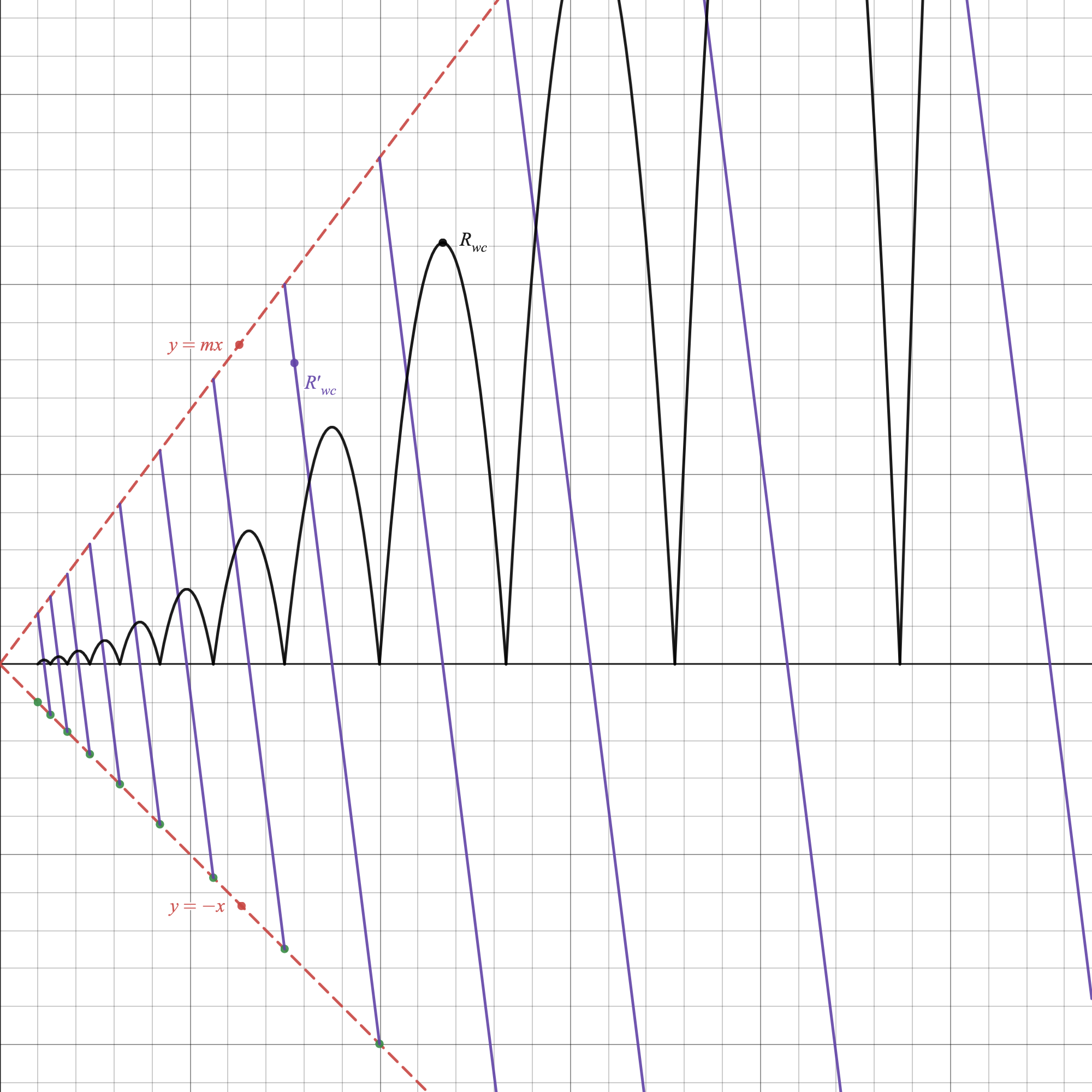
Figure 3: Example of a positive weakly convex function with $\gamma>2\mu$ and unbounded stationary points.

Appendix D Proofs and a counterexample for Section 3

D.1 Proof of Theorem 3.3

Proof.

One of the main limitations in achieving provable stability and convergence guarantees lies in the ability of proving boundedness of iterates $x_{k}$. However, thanks to the form of the regulariser, this is achieved almost immediately. By Lemma B.1, for all $u\in\operatorname{\mathcal{X}}$,

$$\left\langle\partial R_{sc}(x_{k})-\partial R_{sc}(u),x_{k}-u\right\rangle_{\operatorname{\mathcal{X}}^{*}\times\operatorname{\mathcal{X}}}\geqslant\mu\|x_{k}-u\|_{\operatorname{\mathcal{X}}}^{2}$$

and for $\operatorname{\mathcal{D}}$ convex: for all $x,z\in\operatorname{\mathcal{X}}$ and $y\in\operatorname{\mathcal{Y}}$,

$$\operatorname{\mathcal{D}}(\operatorname{\mathcal{A}}z,y)\geqslant\operatorname{\mathcal{D}}(\operatorname{\mathcal{A}}z,y)-\operatorname{\mathcal{D}}(\operatorname{\mathcal{A}}x,y)\geqslant\langle\partial_{x}\operatorname{\mathcal{D}}(\operatorname{\mathcal{A}}x,y),z-x\rangle_{\operatorname{\mathcal{X}}^{*}\times\operatorname{\mathcal{X}}}$$

For any critical point $x_{k}$ and $z\in\operatorname{\mathcal{X}}$, we have:

$$0 \in\left\langle\partial_{x}\operatorname{\mathcal{D}}(\operatorname{\mathcal{A}}x_{k},y_{k})+\alpha\left(\partial\mathcal{R}_{wc}(x_{k})+\partial\mathcal{R}_{sc}(x_{k})\right),z-x_{k}\right\rangle_{\operatorname{\mathcal{X}}^{*}\times\operatorname{\mathcal{X}}}$$

$$\subseteq\langle\partial_{x}\operatorname{\mathcal{D}}(\operatorname{\mathcal{A}}x,y),z-x\rangle_{\operatorname{\mathcal{X}}^{*}\times\operatorname{\mathcal{X}}}-\alpha\left\langle\partial\operatorname{\mathcal{R}}_{sc}(x_{k})-\partial\operatorname{\mathcal{R}}_{sc}(z),x_{k}-z\right\rangle_{\operatorname{\mathcal{X}}^{*}\times\operatorname{\mathcal{X}}}+\alpha\left\langle\partial\operatorname{\mathcal{R}}_{wc}(x_{k})+\partial\operatorname{\mathcal{R}}_{sc}(z),z-x_{k}\right\rangle_{\operatorname{\mathcal{X}}^{*}\times\operatorname{\mathcal{X}}}$$

$$\leqslant\operatorname{\mathcal{D}}(\operatorname{\mathcal{A}}z,y_{k})-\alpha\left\langle\partial\operatorname{\mathcal{R}}_{sc}(x_{k})-\partial\operatorname{\mathcal{R}}_{sc}(z),x_{k}-z\right\rangle_{\times\operatorname{\mathcal{X}}}+\alpha\left\langle\partial\operatorname{\mathcal{R}}_{wc}(x_{k})+\partial\operatorname{\mathcal{R}}_{sc}(z),z-x_{k}\right\rangle_{\operatorname{\mathcal{X}}}.$$

Therefore, since $\gamma<2\mu$, by Theorem 2.6 and by rearranging and completing the square, we get:

$$\left(\|x_{k}-z\|_{\operatorname{\mathcal{X}}}-\frac{1}{2(\mu-\frac{\gamma}{2})}\left(\|\partial\operatorname{\mathcal{R}}_{sc}(z)\|\right)\right)^{2}\leqslant\frac{1}{\alpha(\mu-\frac{\gamma}{2})}\operatorname{\mathcal{D}}(\operatorname{\mathcal{A}}z,y_{k})+\frac{1}{4(\mu-\frac{\gamma}{2})^{2}}\left(\|\partial\operatorname{\mathcal{R}}_{sc}(z)\|\right)^{2}+\frac{1}{(\mu-\frac{\gamma}{2})}\operatorname{\mathcal{R}}_{wc}(z),$$ (D.1)

which together with convergence of $y_{k}$ and continuity of $\operatorname{\mathcal{D}}$ implies that the $(x_{k})$ are bounded, and hence have a weak convergent subsequence since $\operatorname{\mathcal{X}}$ is reflexive, via the Banach–Alaoglu theorem. All that remains is to show that all cluster points $x_{+}$ must be critical points. Passing to a subsequence, let $x_{k}\rightharpoonup x_{+}$. Then in the case of $\gamma\leqslant\mu$:

$$\operatorname{\mathcal{D}}(\operatorname{\mathcal{A}}x_{+},y^{\delta})+\alpha\mathcal{R}(x_{+}) \leqslant\liminf_{k}\operatorname{\mathcal{D}}(\operatorname{\mathcal{A}}x_{k},y_{k})+\alpha\mathcal{R}(x_{k})\quad\text{since $\operatorname{\mathcal{R}}$ and $\operatorname{\mathcal{D}}$ are weakly sequentially l.s.c.}$$

$$\leqslant\liminf_{k}\operatorname{\mathcal{D}}(\operatorname{\mathcal{A}}u,y_{k})+\alpha\mathcal{R}(u)+\frac{\alpha}{2}(\gamma-\mu)\|x_{k}-u\|_{\operatorname{\mathcal{X}}}^{2}\quad\text{$\forall u\in\operatorname{\mathcal{X}}$, by weak convexity}$$

$$\leqslant\operatorname{\mathcal{D}}(\operatorname{\mathcal{A}}u,y^{\delta})+\alpha\mathcal{R}(u)+\frac{\alpha}{2}(\gamma-\mu)\|x_{+}-u\|_{\operatorname{\mathcal{X}}}^{2}\quad\text{ $\forall u\in\operatorname{\mathcal{X}}$,},$$

where the last line follows since $x_{k}\rightharpoonup x_{+}$ and $\|\cdot\|_{\operatorname{\mathcal{X}}}$ is weakly sequentially l.s.c., and therefore $0\in\partial\mathcal{J}_{\alpha,y^{\delta}}(x_{+})$ by definition of weak convexity.

In the case of $\mu<\gamma<2\mu$, $R_{sc}-\frac{1}{2}\mu\|x-u\|_{\operatorname{\mathcal{X}}}^{2}$ weakly sequentially l.s.c.,

$$\operatorname{\mathcal{D}}(\operatorname{\mathcal{A}}x_{+},y^{\delta})+\alpha\mathcal{R}(x_{+})-\frac{\alpha}{2}(\gamma-\mu)\|x_{+}-u\|_{\operatorname{\mathcal{X}}}^{2}$$

$$=\operatorname{\mathcal{D}}(\operatorname{\mathcal{A}}x_{+},y^{\delta})+\alpha\left(\mathcal{R}(x_{+})-\frac{\mu}{2}\|x_{+}-u\|_{\operatorname{\mathcal{X}}}^{2}\right)+\frac{\alpha}{2}(2\mu-\gamma)\|x_{+}-u\|_{\operatorname{\mathcal{X}}}^{2}$$

$$\leqslant\liminf_{k}\operatorname{\mathcal{D}}(\operatorname{\mathcal{A}}x_{k},y_{k})+\alpha\mathcal{R}(x_{k})-\frac{\alpha}{2}(\gamma-\mu)\|x_{k}-u\|_{\operatorname{\mathcal{X}}}^{2}\quad\text{since $\operatorname{\mathcal{R}}-\frac{\mu}{2}\|\cdot-u\|_{\operatorname{\mathcal{X}}}^{2}$, $\|\cdot\|_{\operatorname{\mathcal{X}}}$, and $\operatorname{\mathcal{D}}$ are weakly sequentially l.s.c.}$$

$$\leqslant\liminf_{k}\operatorname{\mathcal{D}}(\operatorname{\mathcal{A}}u,y_{k})+\alpha\mathcal{R}(u)\quad\text{$\forall u\in\operatorname{\mathcal{X}}$, by weak convexity and the criticality of $x_{k}$}$$

$$=\operatorname{\mathcal{D}}(\operatorname{\mathcal{A}}u,y^{\delta})+\alpha\mathcal{R}(u)\quad\text{ $\forall u\in\operatorname{\mathcal{X}}$, since $y_{k}\to y^{\delta}$ and $\operatorname{\mathcal{D}}$ is continuous in its second argument}.$$

∎

D.2 Proof of Theorem 3.4

Proof.

Similar to the theorem above, we first want to show boundedness of iterates $x_{k}$. To achieve this, we use the fact that $y^{0}=\operatorname{\mathcal{A}}u$, and therefore by Assumption 3.1(5)

$$\operatorname{\mathcal{D}}(\operatorname{\mathcal{A}}u,y_{k})\leqslant C\delta_{k}^{p}.$$

Hence, by Equation D.1:

$$\left(\|x_{k}-u\|_{\operatorname{\mathcal{X}}}-\frac{1}{2(\mu-\frac{\gamma}{2})}\left(\|\partial\operatorname{\mathcal{R}}_{sc}(u)\|\right)\right)^{2}\leqslant\frac{C}{\alpha_{k}(\mu-\frac{\gamma}{2})}\delta_{k}^{p}+\frac{1}{4(\mu-\frac{\gamma}{2})^{2}}\left(\|\partial\operatorname{\mathcal{R}}_{sc}(u)\|\right)^{2}+\frac{1}{(\mu-\frac{\gamma}{2})}\operatorname{\mathcal{R}}_{wc}(u),$$

Therefore, as in the previous theorem, $(x_{k})$ weakly has convergent subsequences (due to reflexivity and the Banach–Alaoglu theorem) since $\delta_{k}^{p}/\alpha_{k}$ is assumed to converge. Passing to such a subsequence, let $x_{k}\rightharpoonup x_{+}$. We wish to show that $x_{+}$ is $\operatorname{\mathcal{R}}$-criticising. We first show that $\operatorname{\mathcal{A}}x_{+}=y^{0}$:

$$0\leqslant\operatorname{\mathcal{D}}(\operatorname{\mathcal{A}}x_{+},y) \leqslant\liminf_{k}\operatorname{\mathcal{D}}(\operatorname{\mathcal{A}}x_{k},y_{k})\quad\text{ as $\operatorname{\mathcal{D}}$ is weakly sequentially l.s.c.}$$

$$\leqslant\liminf_{k}\operatorname{\mathcal{D}}(\operatorname{\mathcal{A}}x_{k},y_{k})+\alpha_{k}\mathcal{R}(x_{k})\quad\text{ as $\alpha_{k}\mathcal{R}(x_{k})\geqslant 0$ }$$

$$\leqslant\liminf_{k}\operatorname{\mathcal{D}}(\operatorname{\mathcal{A}}u,y_{k})+\alpha_{k}\mathcal{R}(u)+\frac{1}{2}\alpha_{k}(\gamma-\mu)\|x_{k}-u\|_{\operatorname{\mathcal{X}}}^{2}\quad\text{since $x_{k}\in\operatorname*{crit}\mathcal{J}_{\alpha_{k},y_{k}}$, where $\operatorname{\mathcal{A}}u=y^{0}$}$$

$$\leqslant\liminf_{k}C\delta_{k}^{p}+\alpha_{k}\mathcal{R}(u)+\frac{1}{2}\alpha_{k}(\gamma-\mu)\|x_{k}-u\|_{\operatorname{\mathcal{X}}}^{2}\quad\text{ by \lx@cref{creftypecap~refnum}{assumptions}(5)}$$

$$=0,$$

hence $\operatorname{\mathcal{A}}x_{+}=y^{0}$. It remains to prove that, for all $u\in\operatorname{\mathcal{X}}$ such that $\operatorname{\mathcal{A}}u=y^{0}$,

$$\operatorname{\mathcal{R}}(u)\geqslant\operatorname{\mathcal{R}}(x_{+})+\frac{1}{2}(\mu-\gamma)\|u-x_{+}\|_{\operatorname{\mathcal{X}}}^{2}.$$

By the criticality of $x_{k}$, the positiveness of $\operatorname{\mathcal{D}}$, and Assumption 3.1(5):

$$\alpha_{k}\mathcal{R}(x_{k})\leqslant\operatorname{\mathcal{D}}(\operatorname{\mathcal{A}}x_{k},y_{k})+\alpha_{k}\mathcal{R}(x_{k})\leqslant C\delta_{k}^{p}+\alpha_{k}\mathcal{R}(u)+\frac{1}{2}\alpha_{k}(\gamma-\mu)\|x_{k}-u\|_{\operatorname{\mathcal{X}}}^{2},$$

and so

$$\mathcal{R}(x_{k})\leqslant C\frac{\delta_{k}^{p}}{\alpha_{k}}+\mathcal{R}(u)+\frac{1}{2}(\gamma-\mu)\|x_{k}-u\|_{\operatorname{\mathcal{X}}}^{2}.$$ (D.2)

Therefore, if $\gamma\leqslant\mu$,

$$\operatorname{\mathcal{R}}(x_{+}) \leqslant\liminf_{k}\operatorname{\mathcal{R}}(x_{k})\quad\text{as $\operatorname{\mathcal{R}}$ is weakly sequentially l.s.c.}$$

$$\leqslant\liminf_{k}C\frac{\delta_{k}^{p}}{\alpha_{k}}+\mathcal{R}(u)+\frac{1}{2}(\gamma-\mu)\|x_{k}-u\|_{\operatorname{\mathcal{X}}}^{2}\quad\text{by \lx@cref{creftype~refnum}{eq:Rineq}}$$

$$\leqslant\mathcal{R}(u)+\frac{1}{2}(\gamma-\mu)\|x_{+}-u\|_{\operatorname{\mathcal{X}}}^{2},\quad\text{ since $\|\cdot\|_{\operatorname{\mathcal{X}}}$ is weakly sequentially l.s.c.,}$$

as desired. In the case $\mu<\gamma<2\mu$, $R_{sc}-\frac{1}{2}\mu\|x-u\|_{\operatorname{\mathcal{X}}}^{2}$ is weakly sequentially l.s.c., the proof runs:

$$\operatorname{\mathcal{R}}(x_{+})-\frac{1}{2}\mu\|x_{+}-u\|_{\operatorname{\mathcal{X}}}^{2} \leqslant\liminf_{k}\operatorname{\mathcal{R}}(x_{k})-\frac{1}{2}\mu\|x_{k}-u\|_{\operatorname{\mathcal{X}}}^{2}$$

$$\leqslant\liminf_{k}C\frac{\delta_{k}^{p}}{\alpha_{k}}+\mathcal{R}(u)+\frac{1}{2}(\gamma-2\mu)\|x_{k}-u\|_{\operatorname{\mathcal{X}}}^{2}$$

$$\leqslant\mathcal{R}(u)+\frac{1}{2}(\gamma-2\mu)\|x_{+}-u\|_{\operatorname{\mathcal{X}}}^{2}.$$

Finally, whenever the solution to $\operatorname{\mathcal{A}}u=y^{0}$ is unique, then by the above every subsequence of $x_{k}$ has a subsubsequence converging weakly to that $u$. It follows that $x_{k}$ converges weakly to $u$, as if $x_{k}$ did not converge weakly to $u$, then there would be a neighbourhood $\mathcal{N}$ of $u$ (in the weak topology) and a subsequence $x^{\prime}_{\ell}$ of $x_{k}$ such that $x^{\prime}_{\ell}\notin\mathcal{N}$ for all $\ell$. This subsequence would have no subsubsequence converging weakly to $u$, contradicting the above. ∎

D.3 Counterexample to Theorems 3.3 and 3.4 in the general weakly convex setting

Example D.1.

Let:

• $\operatorname{\mathcal{X}}:=\ell^{2}(\mathbb{N})$, i.e. $\operatorname{\mathcal{X}}:=\{(a_{n})_{n\in\mathbb{N}}:\sum_{n=1}^{\infty}a_{n}^{2}<\infty\}$ with $\langle(a_{n}),(b_{n})\rangle_{\operatorname{\mathcal{X}}}:=\sum_{n=1}^{\infty}a_{n}b_{n}$,

• $\operatorname{\mathcal{Y}}=\mathbb{R}$,

• $\operatorname{\mathcal{A}}=0$,

• $\operatorname{\mathcal{D}}(y,z):=(y-z)^{2}$ (which can be checked to satisfy Assumption 3.1(4-5)) and so $\operatorname{\mathcal{D}}(\operatorname{\mathcal{A}}x,y)=y^{2}$,

• $y_{k}=y^{\delta}=y^{0}=0$, and

• $\operatorname{\mathcal{R}}(x):=\begin{cases}f(x),&\|x\|_{\operatorname{\mathcal{X}}}\leqslant\frac{1}{2},\\ \left(\|x\|^{2}_{\operatorname{\mathcal{X}}}-1\right)^{2},&\|x\|_{\operatorname{\mathcal{X}}}>\frac{1}{2},\end{cases}$ where $f$ is any smooth weakly convex function for which $0$ is not a critical point and for which every derivative (including the $0^{\text{th}}$) of $f$ at any $x$ with $\|x\|_{\operatorname{\mathcal{X}}}=\frac{1}{2}$ agrees with that of $\left(\|x\|^{2}_{\operatorname{\mathcal{X}}}-1\right)^{2}$.

It follows that $\operatorname{\mathcal{R}}$ is weakly convex because there exists $\rho\geqslant 0$ such that $f+\rho\|x\|_{\operatorname{\mathcal{X}}}^{2}$ is convex, and $\left(\|x\|^{2}_{\operatorname{\mathcal{X}}}-1\right)^{2}+2\|x\|_{\operatorname{\mathcal{X}}}^{2}=\|x\|^{4}_{\operatorname{\mathcal{X}}}+1$ is convex since it is the composition of $t\mapsto t^{4}+1$ (which is a convex and monotone on $[0,\infty)$) with $\|\cdot\|_{\operatorname{\mathcal{X}}}$ which is convex and has range $[0,\infty)$. Hence $\operatorname{\mathcal{R}}(x)+\max\{\rho,2\}\|x\|_{\operatorname{\mathcal{X}}}$ is convex.

Then for all $\alpha>0$ and $y\in\operatorname{\mathcal{Y}}$, $\partial\mathcal{J}_{\alpha,y}(x)=\alpha\partial\operatorname{\mathcal{R}}(x)$. Hence, for all $\alpha>0$, $x_{k}\in\operatorname*{crit}_{x\in\operatorname{\mathcal{X}}}\mathcal{J}_{\alpha,y_{k}}$ if and only if $x_{k}\in\operatorname*{crit}_{x\in\operatorname{\mathcal{X}}}\operatorname{\mathcal{R}}$. But by construction $\{\|x\|_{\operatorname{\mathcal{X}}}=1\}\subseteq\operatorname*{crit}_{x\in\operatorname{\mathcal{X}}}\operatorname{\mathcal{R}}$ and $0\notin\operatorname*{crit}_{x\in\operatorname{\mathcal{X}}}\operatorname{\mathcal{R}}$. Therefore, we can choose $x_{k}=e_{k}$, i.e. the sequence which is 1 when $n=k$ and $0$ otherwise. Then it is a well-known fact that $e_{k}\rightharpoonup 0$, which by construction is not a critical point of $\mathcal{J}_{\alpha,y^{\delta}}$. Hence Theorem 3.3 does not hold.

For Theorem 3.4, every $x\in\operatorname{\mathcal{X}}$ has $\operatorname{\mathcal{A}}x=y^{0}$. It follows that $x_{+}$ is an $\operatorname{\mathcal{R}}$-criticising solution if and only if $x_{+}$ is a critical point of $\operatorname{\mathcal{R}}$. We can once again take $x_{k}=e_{k}\in\operatorname*{crit}_{x\in\operatorname{\mathcal{X}}}\mathcal{J}_{\alpha_{k},y_{k}}$, with weak limit 0, which is not a critical point of $\operatorname{\mathcal{R}}$. Hence, Example D.1 is also a counterexample to Theorem 3.4 in the general setting of $\operatorname{\mathcal{R}}$ weak convex.

Note D.2.

The problematic critical points here can be chosen to indeed be global minima of $\operatorname{\mathcal{R}}$, so this issue is not caused by the fact that we are in the setting of critical points.

Note D.3.

We could modify $\operatorname{\mathcal{R}}$ to also be globally Lipschitz by setting $\operatorname{\mathcal{R}}(x)=g(x)$ for $\|x\|_{\operatorname{\mathcal{X}}}>2$ where $g$ is any smooth, globally Lipschitz, weakly convex function whose derivatives all agree with those of $\left(\|x\|^{2}_{\operatorname{\mathcal{X}}}-1\right)^{2}$ at $\|x\|_{\operatorname{\mathcal{X}}}=2$.

Appendix E Proofs and definitions for Section 4

E.1 Proof of Theorem 4.1

Proof.

Written this way, we have by weak convexity-concavity of $L(x,y)$, assuming that $F^{*}$ is $\mu$-strongly convex, that

$$L\left(x^{k+1},y\right)-L\left(x,y^{k+1}\right) =L\left(x^{k+1},y\right)-L\left(x^{k+1},y^{k+1}\right)+L\left(x^{k+1},y^{k+1}\right)-L\left(x,y^{k+1}\right)$$

$$\leqslant\left\langle Tz^{k+1},z^{k+1}-z\right\rangle_{\operatorname{\mathcal{X}}\times\operatorname{\mathcal{Y}}}+\frac{\rho}{2}\|x^{k+1}-x\|_{\operatorname{\mathcal{X}}}^{2}-\frac{\mu}{2}\|y^{k+1}-y\|_{\operatorname{\mathcal{Y}}}^{2}$$

$$=\left\langle z^{k}-z^{k+1},z^{k+1}-z\right\rangle_{M}+\frac{\rho}{2}\|x^{k+1}-x\|_{\operatorname{\mathcal{X}}}^{2}-\frac{\mu}{2}\|y^{k+1}-y\|_{\operatorname{\mathcal{Y}}}^{2}$$ (E.1)

$$=\frac{1}{2}\left\|z^{k}-z\right\|_{M}^{2}-\frac{1}{2}\left\|z^{k+1}-z\right\|_{M}^{2}-\frac{1}{2}\left\|z^{k}-z^{k+1}\right\|_{M}^{2}+\frac{\rho}{2}\|x^{k+1}-x\|_{\operatorname{\mathcal{X}}}^{2}-\frac{\mu}{2}\|y^{k+1}-y\|_{\operatorname{\mathcal{Y}}}^{2}.$$

But then adding together the inequality above for $k$ and $k+1$ evaluated at $z=(x^{k},y^{k+1})$

$$L\left(x^{k+1},y^{k+1}\right)-L\left(x^{k},y^{k}\right) =L\left(x^{k+1},y^{k+1}\right)-L\left(x^{k},y^{k+1}\right)+L\left(x^{k},y^{k+1}\right)-L\left(x^{k},y^{k}\right)$$

$$\leqslant\frac{1}{2}\left\|y^{k}-y^{k+1}\right\|_{M}^{2}-\frac{1}{2}\left\|x^{k+1}-x^{k}\right\|_{M}^{2}-\frac{1}{2}\left\|z^{k}-z^{k+1}\right\|_{M}^{2}+$$

$$\quad-\frac{1}{2}\left\|z^{k-1}-z^{k}\right\|_{M}^{2}+\frac{\rho}{2}\|x^{k+1}-x^{k}\|_{\operatorname{\mathcal{X}}}^{2}-\frac{\mu}{2}\|y^{k+1}-y^{k}\|_{\operatorname{\mathcal{Y}}}^{2}+\frac{1}{2}\left\|\left(\begin{array}[]{c}x^{k-1}-x^{k}\\ y^{k-1}-y^{k+1}\end{array}\right)\right\|_{M}^{2}$$

$$=\left\|y^{k}-y^{k+1}\right\|_{M}^{2}-\frac{1}{2}\left\|x^{k}-x^{k+1}\right\|_{M}^{2}-\frac{1}{2}\left\|z^{k}-z^{k+1}\right\|_{M}^{2}+\frac{\rho}{2}\|x^{k}-x^{k+1}\|_{\operatorname{\mathcal{X}}}^{2}$$

$$\quad-\frac{\mu}{2}\|y^{k+1}-y^{k}\|_{\operatorname{\mathcal{Y}}}^{2}+\left\langle\left(\begin{array}[]{c}x^{k-1}-x^{k}\\ y^{k-1}-y^{k}\end{array}\right),\left(\begin{array}[]{c}0\\ y^{k}-y^{k+1}\end{array}\right)\right\rangle_{M}$$

$$\leqslant\frac{3}{2}\left\|y^{k}-y^{k+1}\right\|_{M}^{2}-\frac{1}{2}\left\|x^{k+1}-x^{k}\right\|_{M}^{2}-\frac{1}{2}\left\|z^{k}-z^{k+1}\right\|_{M}^{2}+$$

$$\quad+\frac{1}{2}\left\|z^{k-1}-z^{k}\right\|_{M}^{2}+\frac{\rho}{2}\|x^{k+1}-x^{k}\|_{\operatorname{\mathcal{X}}}^{2}-\frac{\mu}{2}\|y^{k+1}-y^{k}\|_{\operatorname{\mathcal{Y}}}^{2}.$$

We can write this illustrating descent:

$$L\left(x^{k+1},y^{k+1}\right)+\frac{1}{2}\left\|z^{k}-z^{k+1}\right\|_{M}^{2}+\left[\frac{1}{2}(\mu\sigma-3)\left\|y^{k}-y^{k+1}\right\|_{M}^{2}+\frac{1}{2}(1-\rho\tau)\left\|x^{k+1}-x^{k}\right\|_{M}^{2}\right]\leqslant L\left(x^{k},y^{k}\right)+\frac{1}{2}\left\|z^{k-1}-z^{k}\right\|_{M}^{2}.$$

This becomes descent for the following restrictions on the parameters:

$$\begin{cases}\tau\sigma<\frac{1}{\|\operatorname{\mathcal{A}}\|^{2}},\\ \tau\rho<1,\\ \mu\sigma>3.\end{cases}$$

∎

E.2 Proof of Theorem 4.2

Proof.

In analogy with [Bolte et al., 2014], we shall show require two results - one on descent, as in Theorem 4.1, and one on subgradient boundedness, which arises from the following:

$$\left\|\partial\mathcal{L}(z^{k+1},z^{k})\right\| =\left\|\left(\begin{array}[]{c}\left(\begin{array}[]{c}\partial_{x}L(z^{k+1})\\ \partial_{y}L(z^{k+1})\end{array}\right)+M[z^{k+1}-z^{k}]\\ -M[z^{k+1}-z^{k}]\end{array}\right)\right\|$$

$$\leqslant\left\|\left(\begin{array}[]{c}\left(\begin{array}[]{c}\partial_{x}L(z^{k+1})\\ \partial_{y}L(z^{k+1})\end{array}\right)\\ 0\end{array}\right)\right\|+\left\|\left(\begin{array}[]{c}M[z^{k+1}-z^{k}]\\ -M[z^{k+1}-z^{k}]\end{array}\right)\right\|$$

$$=3\|M(z^{k+1}-z^{k})\|.$$

Overall, the proof is similar to that of [Guo et al., 2023] and [Bolte et al., 2014], and only the first part will be shown here, for compactness. Now, from Theorem 4.1:

$$\sum_{k=1}^{K}\left[\frac{1}{2}(\mu\sigma-3)\left\|y^{k}-y^{k+1}\right\|_{M}^{2}+\frac{1}{2}(1-\rho\tau)\left\|x^{k+1}-x^{k}\right\|_{M}^{2}\right]\leqslant\mathcal{L}(z^{1},z^{0})-\mathcal{L}(z^{K+1},z^{K}).$$

But by assumptions above $\inf_{k}L(x_{k},y_{k})>-\infty$ and by boundedness $\mathcal{L}^{k}>-\infty$, we have $\mathcal{L}^{k}$ is non-increasing and thus converges to $\mathcal{L}^{*}$. Thus, taking $K\to\infty$:

$$\sum_{k=1}^{\infty}\left[\frac{1}{2}(\mu\sigma-3)\left\|y^{k}-y^{k+1}\right\|_{M}^{2}+\frac{1}{2}(1-\rho\tau)\left\|x^{k+1}-x^{k}\right\|_{M}^{2}\right]\leqslant\mathcal{L}^{0}-\mathcal{L}^{*}.$$

This, in particular, implies that the series is square-summable and furthermore that

$$\lim_{k\rightarrow\infty}\left\|x^{k+1}-x^{k}\right\|_{\operatorname{\mathcal{X}}}=0\text{ and }\lim_{k\rightarrow\infty}\left\|y^{k+1}-y^{k}\right\|_{\operatorname{\mathcal{Y}}}=0.$$

Recalling that $\operatorname{dist}\left(0,\partial L(z_{k})\right)=\operatorname{dist}\left(0,T(z_{k})\right)=\left\|z^{k+1}-z^{k}\right\|_{M}\leqslant\left\|y^{k+1}-y^{k}\right\|_{M}+\left\|x^{k+1}-x^{k}\right\|_{M}\to 0$ as $k\to\infty$, and for $\nu=\min\{\mu\sigma-3,1-\rho\tau\}$:

$$\frac{\nu}{4}\left\|z^{k+1}-z^{k}\right\|^{2}_{M}\leqslant\left[\frac{1}{2}(\mu\sigma-3)\left\|y^{k}-y^{k+1}\right\|_{M}^{2}+\frac{1}{2}(1-\rho\tau)\left\|x^{k+1}-x^{k}\right\|_{M}^{2}\right].$$

But also from above we find that

$$\min_{k}\left[\frac{1}{2}(\mu\sigma-3)\left\|y^{k}-y^{k+1}\right\|_{M}^{2}+\frac{1}{2}(1-\rho\tau)\left\|x^{k+1}-x^{k}\right\|_{M}^{2}\right]\leqslant\frac{1}{K}\left(\mathcal{L}(z^{1},z^{0})-\mathcal{L}(z^{K+1},z^{K})\right).$$

Which we can combine to find:

$$\min_{k}\operatorname{dist}\left(0,\partial L(z_{k})\right)\leqslant\frac{2}{(\nu K)^{1/2}}\sqrt{\mathcal{L}(z^{1},z^{0})-\mathcal{L}(z^{K+1},z^{K})}.$$

∎

E.3 The Kurdyka–Łojasiewicz inequality

In [Kurdyka, 1998] Kurdyka provided a generalisation of the Łojasiewicz inequality, with extensions to the nonsmooth setting in [Bolte et al., 2007].

Definition E.1.

Let $\eta\in(0,+\infty]$. Denote with $\Phi_{\eta}$ the set of all concave and continuous functions $\varphi:[0,\eta)\rightarrow[0,+\infty)$ which satisfy: $\varphi(0)=0$; $\varphi$ is $\mathcal{C}^{1}$ on $(0,\eta)$ and continuous at 0; and for all $s\in(0,\eta)$, $\varphi^{\prime}(s)>0$.

Definition E.2.

Let $\Psi:\mathbb{R}^{d}\rightarrow\mathbb{R}\cup\{+\infty\}$ be proper and lower semicontinuous (l.s.c.). Then $\Psi$ is said to have the Kurdyka–Łojasiewicz (KŁ) property at a point $\hat{v}\in\operatorname{dom}\partial\Psi:=$ $\left\{v\in\mathbb{R}^{d}:\partial\Psi(v)\neq\varnothing\right\}$, if there exists $\eta\in(0,+\infty]$, a neighborhood $V$ of $\hat{v}$, and a function $\varphi\in\Phi_{\eta}$ such that for any

$$v\in V\cap\left\{v\in\operatorname{\mathcal{X}}:\Psi(\widehat{v})<\Psi(v)<\Psi(\widehat{v})+\eta\right\}$$

the Kurdyka–Łojasiewicz inequality holds

$$\varphi^{\prime}(\Psi(v)-\Psi(\widehat{v}))\cdot\operatorname{dist}(\mathbf{0},\partial\Psi(v))\geqslant 1.$$

If $\varphi(s)=cs^{1-\theta}$ for $c>0$ and $\theta\in[0,1)$, then $\theta$ is called the KŁ exponent of $\Psi$ at $\hat{v}$. If $\Psi$ has the KŁ property at each point of $\operatorname{dom}\partial\Psi$, then $\Psi$ is called a KŁ function (or just, KŁ).

Examples of KŁ functions include semialgebraic, subanalytic, uniformly convex functions (see [Attouch et al., 2010] and the references therein) and all typical neural networks.

Theorem E.3.

Let $\Psi:\mathbb{R}^{d}\rightarrow\mathbb{R}$ be a deep neural network with every activation function a continuous piecewise analytic function with finitely many pieces (e.g., ReLU, sigmoid). Then $\Psi$ is a KŁ function and for all $\hat{v}\in\operatorname{dom}\partial\Psi$, there exists $\theta\in[0,1)$ such that $\Psi$ has KŁ exponent $\theta$ at $\hat{v}$.

Proof.

The network $\Psi$ is a finite composition of continuous piecewise analytic functions with finitely many pieces, and hence is a continuous piecewise analytic function with finitely many pieces. It follows that $\Psi$ is subanalytic and so the result follows by Theorem 3.1 of [Bolte et al., 2007]. ∎

E.4 Proof of Theorem 4.5

Before providing the proof, we are first going to provide two lemmas:

Lemma E.4.

For $f:\operatorname{\mathcal{X}}\rightarrow\mathbb{R}$ $\rho$-convex and $x_{1:N}\in\operatorname{\mathcal{X}}$, and $\bar{\;\cdot\;}$ denoting an average,

$$f(\bar{x})\leqslant\bar{f}-\frac{{\rho}}{2N}\sum_{i=1}^{N}\frac{i-1}{i}\|x^{i}-\bar{x}^{i-1}\|_{\operatorname{\mathcal{X}}}^{2},$$

and furthermore emphasising the weak convex case, for any $x\in\operatorname{\mathcal{X}}$:

$$f(\bar{x})\leqslant\bar{f} +\max{(0,-\rho)}\cdot\left[\frac{1}{N}\sum_{i=1}^{N}\|x^{i}-x\|_{\operatorname{\mathcal{X}}}^{2}+\frac{1}{N}\sum_{i=1}^{N}\frac{1}{i}\sum^{i-1}_{j=1}\|x^{j}-x\|_{\operatorname{\mathcal{X}}}^{2}\right].$$

Proof.

This arises from the following fact for $\rho$-convex functions:

$$\begin{split}f\left(\frac{1}{N}\left(x_{1}+\dots+x_{N}\right)\right)&\leqslant\frac{1}{N}f(x_{N})-\frac{\rho}{2}\frac{1}{N}\left(1-\frac{1}{N}\right)\|x_{n}-\bar{x}_{n-1}\|_{\operatorname{\mathcal{X}}}^{2}\\ &\qquad\qquad+\frac{N-1}{N}f\left(\frac{1}{N-1}\left(x_{1}+\dots+x_{N-1}\right)\right)\\ &\leqslant\dots\leqslant\bar{f}-\frac{\rho}{2N}\sum_{i=1}^{k}\frac{i-1}{i}\|x_{i}-\bar{x}_{i-1}\|_{\operatorname{\mathcal{X}}}^{2}.\end{split}$$ (E.2)

To arrive at the second result we wish to expand the last term in terms of iterate lengths:

$$\sum_{i=1}^{N}\frac{i-1}{i}\|x_{i}-\bar{x}_{i-1}\|_{\operatorname{\mathcal{X}}}^{2} \leqslant 2\sum_{i=1}^{N}\frac{i-1}{i}\left(\|x_{i}-x\|_{\operatorname{\mathcal{X}}}^{2}+\|x-\bar{x}_{i-1}\|_{\operatorname{\mathcal{X}}}^{2}\right)$$

$$\leqslant 2\sum_{i=1}^{N}\frac{i-1}{i}\left(\|x_{i}-x\|_{\operatorname{\mathcal{X}}}^{2}+\left\|\frac{1}{i-1}\sum_{j=1}^{i-1}\left(x_{j}-x\right)\right\|_{\operatorname{\mathcal{X}}}^{2}\right)$$

By Jensen’s inequality: $$\leqslant 2\sum_{i=1}^{N}\frac{i-1}{i}\left(\|x_{i}-x\|_{\operatorname{\mathcal{X}}}^{2}+\frac{1}{i-1}\sum^{i-1}_{j=1}\|x_{j}-x\|_{\operatorname{\mathcal{X}}}^{2}\right).$$

Plugging this into Equation E.2 yields the desired result. ∎

And now by application of Lemma E.4 to $L$:

Lemma E.5.

Let $\bar{z}^{k}:=\left(\bar{x}^{k},\bar{y}^{k}\right):=\frac{1}{k}\sum_{i=1}^{k}z^{i}$ be the average iterate. Assuming that $L(x,y)$ is $\rho$-convex in the first argument and $\mu$-concave in the second, for any $k\geqslant 1$ and z:

$$L\left(\bar{x}^{k},y\right)-L\left(x,\bar{y}^{k}\right) \leqslant\frac{\left\|z-z^{0}\right\|_{M}^{2}}{2k}-\frac{1}{2k}\sum_{i=1}^{k}\|z^{i-1}-z^{i}\|_{M}^{2}$$

$$\quad-\frac{\rho}{2k}\sum_{i=1}^{k}\|x^{i}-x\|_{\operatorname{\mathcal{X}}}^{2}-\frac{\rho}{2k}\sum_{i=1}^{k}\frac{i-1}{i}\|x^{i}-\bar{x}^{i-1}\|_{\operatorname{\mathcal{X}}}^{2}$$

$$\quad-\frac{\mu}{2k}\sum_{i=1}^{k}\|y^{i}-y\|_{\operatorname{\mathcal{Y}}}^{2}-\frac{\mu}{2k}\sum_{i=1}^{k}\frac{i-1}{i}\|y^{i}-\bar{y}^{i-1}\|_{\operatorname{\mathcal{Y}}}^{2}.$$

Further, setting $D=\operatorname{diag}\left(\max{(0,-\rho)},\max{(0,-\mu)}\right)$:

$$L\left(\bar{x}^{k},y\right)-L\left(x,\bar{y}^{k}\right)\leqslant\frac{\left\|z-z^{0}\right\|_{M}^{2}}{2k}+\frac{3}{2k}\sum_{i=1}^{k}\|z^{i}-z\|_{D}^{2}+\frac{1}{k}\sum_{i=1}^{k}\frac{1}{i}\sum^{i-1}_{j=1}\|z^{j}-z\|_{D}^{2}.$$

Proof.

We can expand the original as:

$$L\left(\bar{x}^{k},y\right)-L\left(x,\bar{y}^{k}\right)=\left(L\left(\bar{x}^{k},y\right)-L\left(x,y\right)\right)+\left(L\left(x,y\right)-L\left(x,\bar{y}^{k}\right)\right)$$

Noting that the first bracket is convex in $\bar{x}^{k}$ and second is convex in $\bar{y}^{k}$, we can use Lemma E.4 to bound:

$$L\left(\bar{x}^{k},y\right)-L\left(x,\bar{y}^{k}\right) =\left(L\left(\bar{x}^{k},y\right)-L\left(x,y\right)\right)+\left(L\left(x,y\right)-L\left(x,\bar{y}^{k}\right)\right)$$

$$\leqslant\frac{1}{k}\sum_{i=1}^{k}L\left(x^{i},y\right)-L\left(x,y^{i}\right)$$

$$\qquad-\frac{\rho}{2k}\sum_{i=1}^{k}\|x^{i}-x\|_{\operatorname{\mathcal{X}}}^{2}-\frac{\rho}{2k}\sum_{i=1}^{k}\frac{i-1}{i}\|x^{i}-\bar{x}^{i-1}\|_{\operatorname{\mathcal{X}}}^{2}$$

$$\qquad-\frac{\mu}{2k}\sum_{i=1}^{k}\|y^{i}-y\|_{\operatorname{\mathcal{Y}}}^{2}-\frac{\mu}{2k}\sum_{i=1}^{k}\frac{i-1}{i}\|y^{i}-\bar{y}^{i-1}\|_{\operatorname{\mathcal{Y}}}^{2}$$

by Equation E.1 $$\leqslant\frac{\left\|z-z^{0}\right\|_{M}^{2}}{2k}-\frac{1}{2k}\sum_{i=1}^{k}\|z^{i-1}-z^{i}\|_{M}^{2}$$

$$\qquad-\frac{\rho}{2k}\sum_{i=1}^{k}\|x^{i}-x\|_{\operatorname{\mathcal{X}}}^{2}-\frac{\rho}{2k}\sum_{i=1}^{k}\frac{i-1}{i}\|x^{i}-\bar{x}^{i-1}\|_{\operatorname{\mathcal{X}}}^{2}$$

$$\qquad-\frac{\mu}{2k}\sum_{i=1}^{k}\|y^{i}-y\|_{\operatorname{\mathcal{Y}}}^{2}-\frac{\mu}{2k}\sum_{i=1}^{k}\frac{i-1}{i}\|y^{i}-\bar{y}^{i-1}\|_{\operatorname{\mathcal{Y}}}^{2}$$

Using the second part of Lemma E.4, we can arrive at the second result:

$$L\left(\bar{x}^{k},y\right)-L\left(x,\bar{y}^{k}\right) \leqslant\frac{\left\|z-z^{0}\right\|_{M}^{2}}{2k}-\frac{\rho}{2k}\sum_{i=1}^{k}\|x^{i}-x\|_{\operatorname{\mathcal{X}}}^{2}-\frac{\mu}{2k}\sum_{i=1}^{k}\|y^{i}-y\|_{\operatorname{\mathcal{Y}}}^{2}$$

$$\qquad+\max{(0,-\rho)}\cdot\left[\frac{1}{k}\sum_{i=1}^{k}\|x^{i}-x\|_{\operatorname{\mathcal{X}}}^{2}+\frac{1}{k}\sum_{i=1}^{k}\frac{1}{i}\sum^{i-1}_{j=1}\|x^{j}-x\|_{\operatorname{\mathcal{X}}}^{2}\right]$$

$$\qquad+\max{(0,-\mu)}\cdot\left[\frac{1}{k}\sum_{i=1}^{k}\|y^{i}-y\|_{\operatorname{\mathcal{Y}}}^{2}+\frac{1}{k}\sum_{i=1}^{k}\frac{1}{i}\sum^{i-1}_{j=1}\|y^{j}-y\|_{\operatorname{\mathcal{Y}}}^{2}\right]$$

Yielding the desired result. ∎

Now, with the lemmas above we can prove Theorem 4.5.

Proof of Theorem 4.5.

Using $\mu$-strong concavity in the second argument and $\rho$-weak convexity in the first, and using that $\hat{z}$ is a stationary point of $L$, we can bound:

$$L\left(\bar{x}^{k},y\right)-L\left(x,\bar{y}^{k}\right)\leqslant-\frac{\mu}{2}\|y-\hat{y}\|_{\operatorname{\mathcal{Y}}}^{2}+\frac{\rho}{2}\|x-\hat{x}\|_{\operatorname{\mathcal{X}}}^{2}+L\left(\bar{x}^{k},\hat{y}\right)-L\left(\hat{x},\bar{y}^{k}\right).$$

Now, from the second part of Lemma E.5 we have

$$L\left(\bar{x}^{k},\hat{y}\right)-L\left(\hat{x},\bar{y}^{k}\right)\leqslant\frac{\left\|\hat{z}-z^{0}\right\|_{M}^{2}}{2k}+\frac{3}{2k}\sum_{i=1}^{k}\|z^{i}-\hat{z}\|_{D}^{2}+\frac{1}{k}\sum_{i=1}^{k}\frac{1}{i}\sum^{i-1}_{j=1}\|z^{j}-\hat{z}\|_{D}^{2},$$

while from Theorem 4.4 (by redefining the constants appropriately), then we have constants $\nu>0,0<\tau<1$, such that

$$\left\|z^{k}-\hat{z}\right\|_{D}\leqslant\nu\tau^{k},$$

which in turn implies the following two bounds:

$$\frac{1}{k}\sum_{i=1}^{k}\|z^{i}-\hat{z}\|_{D}^{2}\leqslant\frac{1}{k}\nu^{2}\sum_{i=1}^{k}\tau^{2k}=\frac{1}{k}\nu^{2}\tau^{2}\frac{1-\tau^{2k}}{1-\tau^{2}}=\mathcal{O}\left(\frac{1}{k}\right)$$

and

$$\frac{1}{k}\sum_{i=1}^{k}\frac{1}{i}\sum^{i-1}_{j=1}\|z^{j}-\hat{z}\|_{D}^{2} \leqslant\frac{1}{k}\nu^{2}\tau^{2}\sum_{i=1}^{k}\frac{1}{i}\cdot\frac{1-\tau^{2(i-1)}}{1-\tau^{2}}$$

$$\leqslant\frac{1}{k}\frac{\nu^{2}\tau^{2}}{1-\tau^{2}}\sum_{i=1}^{k}\frac{1}{i}\leqslant\frac{\nu^{2}\tau^{2}}{1-\tau^{2}}\frac{\log{k}+1}{k}=\mathcal{O}\left(\frac{\log{k}}{k}\right),$$

by a standard inequality bounding harmonic series.

If instead $\theta\in\left(\frac{1}{2},1\right)$, then there exist a constant $\mu>0$,

$$\left\|z^{k}-\hat{z}\right\|_{D}\leqslant\mu k^{-\frac{1-\theta}{2\theta-1}}.$$

But this implies the following two bounds:

$$\frac{1}{k}\sum_{i=1}^{k}\|z^{i}-\hat{z}\|_{D}^{2}\leqslant\frac{1}{k}\mu^{2}\sum_{i=1}^{k}i^{-2\frac{1-\theta}{2\theta-1}}\leqslant\frac{1}{k}\mu^{2}\zeta\left(2\frac{1-\theta}{2\theta-1}\right)=\mathcal{O}\left(\frac{1}{k}\right)$$

and

$$\frac{1}{k}\sum_{i=1}^{k}\frac{1}{i}\sum^{i-1}_{j=1}\|z^{j}-\hat{z}\|_{D}^{2} \leqslant\frac{1}{k}\sum_{i=1}^{k}\frac{1}{i}\mu^{2}\zeta\left(2\frac{1-\theta}{2\theta-1}\right)$$

$$\leqslant\frac{1}{k}\mu^{2}\zeta\left(2\frac{1-\theta}{2\theta-1}\right)(\log{k}+1)=\mathcal{O}\left(\frac{\log k}{k}\right),$$

where $\zeta$ denotes the Riemann zeta function.

Now, if $\theta=0$, denoting $\sum_{i=1}^{\infty}\|z^{i}-\hat{z}\|_{D}^{2}$ as $d$, which is guarranteed to be finite, since we converge in a finite number of steps by Theorem 4.4, we have:

$$\frac{1}{k}\sum_{i=1}^{k}\|z^{i}-\hat{z}\|_{D}^{2}\leqslant\frac{d}{k}=\mathcal{O}\left(\frac{1}{k}\right)\quad$$

and

$$\frac{1}{k}\sum_{i=1}^{k}\frac{1}{i}\sum^{i-1}_{j=1}\|z^{j}-\hat{z}\|_{D}^{2} \leqslant\frac{1}{k}\sum_{i=1}^{k}\frac{1}{i}d\leqslant d\frac{\log{k}+1}{k}=\mathcal{O}\left(\frac{\log{k}}{k}\right).$$

Therefore, in all three cases we achieve the following bound:

$$L\left(\bar{x}^{k},y\right)-L\left(x,\bar{y}^{k}\right)\leqslant\frac{1}{2}\|z-\hat{z}\|_{D}^{2}+\mathcal{O}\left(\frac{\log k}{k}\right).$$

∎

Appendix F Proof of Theorem 5.2

Before we can move onto proof of Theorem 5.2, we are going to need to establish a number of results relating to both universal approximation properties of standard neural networks, as well as approximation properties of Moreau envelopes.

Lemma F.1 (Lemma 3 in [Strömberg, 1996]).

Let $f$ be a proper extended-real-valued l.s.c. bounded below function on $\operatorname{\mathcal{X}}$.

For any $t>0$ it holds that

• $f_{t}$ is a real-valued minorant of $f$;

• $\inf f_{t}=\inf f$;

• $\arg\min f_{t}=\arg\min f$.

Furthermore, when $t\downarrow 0$:

• $f_{t}\rightarrow f$ pointwise;

• $f_{t}\rightarrow f$ with respect to the epi-distance topology provided $\|\cdot\|_{\operatorname{\mathcal{X}}}$ is uniformly rotund;

• $f_{t}\rightarrow f$ uniformly on bounded sets when $f$ is uniformly continuous on bounded sets and $\|\cdot\|_{\operatorname{\mathcal{X}}}$ is uniformly rotund.

Note, that e.g. the Euclidean norm is uniformly rotund. In what follows we use point (vi) in order to approximate the desired function with a weak convex smooth approximant.

Theorem F.2 (Representation power of ICNN; Theorem 1 in [Chen et al., 2019]).

For any Lipschitz convex function over a compact domain, there exists a neural network with nonnegative weights and ReLU activation functions (i.e., an ICNN) that approximates it uniformly within $\varepsilon$, i.e. in the $\|\cdot\|_{\infty}$ norm.

A further summary can be found in [Hanin, 2019]. The last piece for the proof of universal approximation of IWCNNs is a universal approximation results for a neural network with smooth activations:

Theorem F.3 (Theorem 3.2 in [Kidger and Lyons, 2020]).

Let $\rho:\mathbb{R}\rightarrow\mathbb{R}$ be any nonaffine continuous function which is continuously differentiable at at least one point, with nonzero derivative at that point. Let $K\subseteq\mathbb{R}^{n}$ be compact. Then $\mathcal{NN}_{n,m,n+m+2}^{\rho}$ is dense in $C\left(K;\mathbb{R}^{m}\right)$ with respect to the uniform norm.

Here $\mathcal{NN}_{n,m,n+m+2}^{\rho}$ represents the class of functions $\mathbb{R}^{n}\to\mathbb{R}^{m}$ described by feedforward neural networks with $n$ neurons in the input layer, $m$ neurons in the output layer, and an arbitrary number of hidden layers, each with $n+m+2$ neurons and activation function $\rho$ as in [Kidger and Lyons, 2020].

With these results, we can now prove Theorem 5.2.

Proof of Theorem 5.2.

Fix $\varepsilon>0$. Consider some target proper extended-real-valued l.s.c. function $f\in\mathcal{C}_{0}(X)$, with $X$ compact. Then, by [Sun and Yu, 2019] Theorem 6, there exists $f_{wc}\in\mathcal{WC}(X)\cap\mathcal{C}_{0}(X)$ with $\|f-f_{wc}\|_{\infty}<\frac{\varepsilon}{2}$. In fact, we know exactly how to find such approximation using the Moreau envelope: $f_{wc}=f_{t}$ for some $t>0$ by Lemma F.1, which furthermore is Lipschitz smooth by Theorem A.3. As a result, we can write $f_{wc}=\operatorname{Id}\circ\;f_{t}$. Now, more generically for $m\neq 1$, we can e.g. consider just the first element, i.e. $g^{\textrm{conv}}:x\to x_{1}$ and $g^{\textrm{sm}}:x\to(e_{t}f,0,\cdots,0)^{\top}$, with $f_{wc}=g^{\textrm{conv}}\circ g^{\textrm{sm}}$.

By Theorem F.3 there exists a neural network such that $\|g^{\textrm{sm}}_{\theta_{2}}-g^{\textrm{sm}}\|_{\infty}<\frac{\varepsilon}{2}$. Since $g^{\textrm{sm}}_{\theta_{2}}$ is continuous and $X$ is compact, $g^{\textrm{sm}}_{\theta_{2}}(X)$ is compact. Therefore, by Theorem F.2, as $g^{\textrm{conv}}$ is Lipschitz convex, there exists an ICNN such that $\|g^{\textrm{ICNN}}_{\theta_{1}}-g^{\textrm{conv}}\|_{\infty}<\frac{\varepsilon}{2}$ on $\operatorname{Im}g^{\textrm{sm}}_{\theta_{2}}$. Therefore,

$$\|g^{\textrm{ICNN}}_{\theta_{1}}\circ g^{\textrm{sm}}_{\theta_{2}}-g^{\textrm{conv}}\circ g^{\textrm{sm}}\|_{\infty} \leqslant\|g^{\textrm{ICNN}}_{\theta_{1}}\circ g^{\textrm{sm}}_{\theta_{2}}-g^{\textrm{conv}}\circ g^{\textrm{sm}}_{\theta_{2}}\|_{\infty}+\|g^{\textrm{conv}}\circ g^{\textrm{sm}}_{\theta_{2}}-g^{\textrm{conv}}\circ g^{\textrm{sm}}\|_{\infty}$$

$$\leqslant\|g^{\textrm{ICNN}}_{\theta_{1}}-g^{\textrm{conv}}\|_{\infty}+\|g^{\textrm{sm}}_{\theta_{2}}-g^{\textrm{sm}}\|_{\infty}$$

$$<\varepsilon,$$

by 1-Lipschitzness of $g^{\textrm{conv}}$. Therefore, IWCNNs are dense in the space of continuous functions. ∎

Appendix G Experimental set-up and additional data visualisations for Section 6

G.1 Experimental set-up

We use human abdominal CT scans for 10 patients provided by Mayo Clinic for the low-dose CT grand challenge [McCollough, 2014]. The training dataset for CT experiments consists of a total of 2250 2D slices, each of dimension $512\times 512$, corresponding to 9 patients. The remaining 128 slices corresponding to one patient are used to evaluate the reconstruction performance.

Projection data is simulated in ODL [Adler et al., 2017] with a GPU-accelerated astra back-end, using a parallel-beam acquisition geometry with 350 angles and 700 rays/angle, using additive Gaussian noise with $\sigma=3.2$. The pseudoinverse reconstruction is taken to be images obtained using FBP. For limited angle experiments, data is simulated with a missing angular wedge of 60^∘. The native odl power method is used to approximate the norm of the operator.

The TV method was computed by employing the ADMM-based solver in ODL.

All of the methods are implemented in PyTorch [Paszke et al., 2017]. The LPD method is trained on pairs of target images and projected data, while the U-Net post-processor is trained on pairs of true images and the corresponding reconstructed FBPs. AR, ACR, ACNCR, and AWCR, in contrast, require ground-truth and FBP images drawn from their marginal distributions (and hence not necessarily paired). The hyperparameter $\lambda$ from Equation 5.1 is chosen to be the same as in [Mukherjee et al., 2021]. To aid with training, $\mu$ from Definition 5.5 is first chosen to be small (0.1) and once the network is trained is increased to a larger value (10) as in [Mukherjee et al., 2021, Lunz et al., 2018]), and the network is fine-tuned. The RMSprop optimizer, following the recommendation in [Lunz et al., 2018, Mukherjee et al., 2021] with a learning rate of $5\times 10^{-5}$ is used for training for a total of 50 epochs. For fine-tuning, the learning rate is reduced to $10^{-6}$. The AWCR architecture differed for the two experiments in the following way:

Sparse view CT The ICNN component of the AWCR is constructed with 5 convolutional layers, using LeakyReLU activations and $5\times 5$ kernels with 16 channels. The smooth component of the AWCR is constructed using 6 convolutional layers, using nn.SiLU activations and $5\times 5$ kernels with a doubling number of channels from 16 and stride of 2, similar to that of [Lunz et al., 2018], with the last layer containing 128 channels

Limited view CT The ICNN component of the AWCR is constructed with 5 convolutional layers, using LeakyReLU activations and $5\times 5$ kernels with 16 channels. Guided by the observations of [Mukherjee et al., 2021], that reducing the total number of layers and the number of feature channels helps avoid overfitting in the limited angle setting, the smooth component of the AWCR is constructed using a single convolutional layers, using a SiLU activation, $5\times 5$ with 128 channels.

The reconstruction in all adversarial regularisation cases is performed by solving the variational problem via gradient-descent for 1000 iterations with a step size of $10^{-6}$. For the AWCR-PD, the primal-dual algorithm is used for solving the variational problem. The proximal operator of the network is approximated by performing gradient descent with backtracking on the objective in Section 4.1. The step sizes are chosen to be equal to $0.1/\|\operatorname{\mathcal{A}}\|$ in the sparse case, and in the limited angle are chosen to be equal to $10/\|\operatorname{\mathcal{A}}\|$ and $0.1/\|\operatorname{\mathcal{A}}\|$ to ensure that iterates do not diverge and that steps are large enough to provide good results. Akin to AR, reconstruction performance of AWCR can sometimes deteriorate if early stopping is not applied. For a fair comparison, we report the highest PSNR achieved by all methods during reconstruction. The regularisation parameter $\alpha$ is chosen according to [Lunz et al., 2018] and is not tuned.

G.2 Additional data visualisations

Ground-truth

FBP: 17.944 dB, 0.193

AWCR: 26.981 dB, 0.789

AWCR-PD: 22.899 dB, 0.694

Figure 4: Reconstructed images obtained using different methods, along with the associated PSNR and SSIM, for sparse view CT. In this case the AWCR and AWCR-PD look significantly different.

References

- [Adler et al., 2017] Adler, J., Kohr, H., and Öktem, O. (2017). Operator discretization library (ODL). Software available from https://github.com/odlgroup/odl.
- [Adler and Öktem, 2018] Adler, J. and Öktem, O. (2018). Learned primal-dual reconstruction. IEEE transactions on medical imaging, 37(6):1322–1332.
- [Alberti et al., 2021] Alberti, G. S., De Vito, E., Lassas, M., Ratti, L., and Santacesaria, M. (2021). Learning the optimal Tikhonov regularizer for inverse problems. Advances in Neural Information Processing Systems, 34:25205–25216.
- [Ambrosio et al., 2005] Ambrosio, L., Gigli, N., and Savaré, G. (2005). Gradient flows: in metric spaces and in the space of probability measures. Lectures in Mathematics. ETH Zürich. Birkhäuser Basel.
- [Amos et al., 2017] Amos, B., Xu, L., and Kolter, J. Z. (2017). Input convex neural networks. In International Conference on Machine Learning, pages 146–155. PMLR.
- [Arjovsky et al., 2017] Arjovsky, M., Chintala, S., and Bottou, L. (2017). Wasserstein GAN.
- [Arridge et al., 2019] Arridge, S., Maass, P., Öktem, O., and Schönlieb, C.-B. (2019). Solving inverse problems using data-driven models. Acta Numerica, 28:1–174.
- [Arrow et al., 1958] Arrow, K. J., Hurwicz, L., and Chenery, H. B. (1958). Studies in linear and non-linear programming. Stanford Mathematical Studies in the Social Sciences. Stanford University Press, Stanford, California.
- [Attouch et al., 2010] Attouch, H., Bolte, J., Redont, P., and Soubeyran, A. (2010). Proximal Alternating Minimization and Projection Methods for Nonconvex Problems: An Approach Based on the Kurdyka-Łojasiewicz Inequality. Mathematics of Operations Research, 35(2):438–457.
- [Beck, 2017] Beck, A. (2017). First-Order Methods in Optimization. Society for Industrial and Applied Mathematics, Philadelphia, PA.
- [Benning and Burger, 2018] Benning, M. and Burger, M. (2018). Modern regularization methods for inverse problems. Acta Numerica, 27:1–111.
- [Böhm and Wright, 2021] Böhm, A. and Wright, S. J. (2021). Variable smoothing for weakly convex composite functions. Journal of optimization theory and applications, 188:628–649.
- [Bolte et al., 2007] Bolte, J., Daniilidis, A., and Lewis, A. (2007). The Łojasiewicz inequality for nonsmooth subanalytic functions with applications to subgradient dynamical systems. SIAM Journal on Optimization, 17(4):1205–1223.
- [Bolte et al., 2014] Bolte, J., Sabach, S., and Teboulle, M. (2014). Proximal alternating linearized minimization for nonconvex and nonsmooth problems. Mathematical Programming, 146(1-2):459–494.
- [Borwein and Lewis, 2006] Borwein, J. and Lewis, A. (2006). Convex Analysis and Nonlinear Optimization. CMS Books in Mathematics. Springer New York, NY, 2nd edition.
- [Bredies et al., 2010] Bredies, K., Kunisch, K., and Pock, T. (2010). Total Generalized Variation. SIAM Journal on Imaging Sciences, 3(3):492–526.
- [Budd et al., 2023] Budd, J. M., van Gennip, Y., Latz, J., Parisotto, S., and Schönlieb, C.-B. (2023). Joint reconstruction-segmentation on graphs. SIAM Journal on Imaging Sciences, 16(2):911–947.
- [Calatroni et al., 2018] Calatroni, L., d’Autume, M., Hocking, R., Panayotova, S., Parisotto, S., Ricciardi, P., and Schönlieb, C.-B. (2018). Unveiling the invisible: mathematical methods for restoring and interpreting illuminated manuscripts. Heritage Science, 6(1).
- [Chambolle and Pock, 2011] Chambolle, A. and Pock, T. (2011). A first-order primal-dual algorithm for convex problems with applications to imaging. Journal of Mathematical Imaging and Vision, 40(1):120–145.
- [Chen and Needell, 2016] Chen, G. and Needell, D. (2016). Compressed sensing and dictionary learning. Proc. Sympos. Appl. Math., 73:201–241.
- [Chen et al., 2019] Chen, Y., Shi, Y., and Zhang, B. (2019). Optimal control via neural networks: A convex approach. In International Conference on Learning Representations.
- [Davis and Drusvyatskiy, 2018] Davis, D. and Drusvyatskiy, D. (2018). Stochastic subgradient method converges at the rate on weakly convex functions. arXiv preprint arXiv:1802.02988.
- [Davis and Drusvyatskiy, 2022] Davis, D. and Drusvyatskiy, D. (2022). Proximal methods avoid active strict saddles of weakly convex functions. Foundations of Computational Mathematics, 22(2):561–606.
- [Davis et al., 2018] Davis, D., Drusvyatskiy, D., MacPhee, K. J., and Paquette, C. (2018). Subgradient methods for sharp weakly convex functions. Journal of Optimization Theory and Applications, 179(3):962–982.
- [Davoli et al., 2023] Davoli, E., Fonseca, I., and Liu, P. (2023). Adaptive image processing: First order PDE constraint regularizers and a bilevel training scheme. Journal of Nonlinear Science, 33(3):41.
- [Dimakis, 2022] Dimakis, A. G. (2022). Deep Generative Models and Inverse Problems, page 400–421. Cambridge University Press.
- [Dittmer et al., 2019] Dittmer, S., Kluth, T., Maass, P., and Baguer, D. O. (2019). Regularization by architecture: A deep prior approach for inverse problems. Journal of Mathematical Imaging and Vision, pages 1–15.
- [Drusvyatskiy and Davis, 2020] Drusvyatskiy, D. and Davis, D. (2020). Subgradient methods under weak convexity and tame geometry. SIAG/OPT Views and News, 28:1–10.
- [Drusvyatskiy and Paquette, 2019] Drusvyatskiy, D. and Paquette, C. (2019). Efficiency of minimizing compositions of convex functions and smooth maps. Mathematical Programming, 178:503–558.
- [Durand and Nikolova, 2006] Durand, S. and Nikolova, M. (2006). Stability of the minimizers of least squares with a non-convex regularization. Part I: Local behavior. Applied Mathematics and Optimization, 53:185–208.
- [Engl et al., 1996] Engl, H. W., Hanke, M., and Neubauer, A. (1996). Regularization of inverse problems, volume 375 of Mathematics and Its Applications. Springer Dordrecht.
- [Gilboa and Osher, 2009] Gilboa, G. and Osher, S. (2009). Nonlocal operators with applications to image processing. Multiscale Modeling & Simulation, 7(3):1005–1028.
- [Goujon et al., 2024] Goujon, A., Neumayer, S., and Unser, M. (2024). Learning weakly convex regularizers for convergent image-reconstruction algorithms. SIAM Journal on Imaging Sciences, 17(1):91–115.
- [Grasmair, 2010] Grasmair, M. (2010). Generalized Bregman distances and convergence rates for non-convex regularization methods. Inverse problems, 26(11):115014.
- [Guo et al., 2023] Guo, J., Wang, X., and Xiao, X. (2023). Preconditioned primal-dual gradient methods for nonconvex composite and finite-sum optimization. arXiv preprint arXiv:2309.13416.
- [Hanin, 2019] Hanin, B. (2019). Universal Function Approximation by Deep Neural Nets with Bounded Width and ReLU Activations. Mathematics, 7(10):992.
- [Hurault et al., 2022] Hurault, S., Leclaire, A., and Papadakis, N. (2022). Proximal denoiser for convergent plug-and-play optimization with nonconvex regularization. In Chaudhuri, K., Jegelka, S., Song, L., Szepesvari, C., Niu, G., and Sabato, S., editors, Proceedings of the 39th International Conference on Machine Learning, volume 162 of Proceedings of Machine Learning Research, pages 9483–9505. PMLR.
- [Jin et al., 2017] Jin, K. H., McCann, M. T., Froustey, E., and Unser, M. (2017). Deep convolutional neural network for inverse problems in imaging. IEEE Transactions on Image Processing, 26(9):4509–4522.
- [Kidger and Lyons, 2020] Kidger, P. and Lyons, T. (2020). Universal Approximation with Deep Narrow Networks. In Abernethy, J. and Agarwal, S., editors, Proceedings of Thirty Third Conference on Learning Theory, volume 125 of Proceedings of Machine Learning Research, pages 2306–2327. PMLR.
- [Krizhevsky et al., 2017] Krizhevsky, A., Sutskever, I., and Hinton, G. E. (2017). Imagenet classification with deep convolutional neural networks. Communications of the ACM, 60(6):84–90.
- [Kurdyka, 1998] Kurdyka, K. (1998). On gradients of functions definable in o-minimal structures. In Annales de l’institut Fourier, volume 48, pages 769–783.
- [Kutyniok and Labate, 2012] Kutyniok, G. and Labate, D. (2012). Multiscale analysis for multivariate data. Springer.
- [Lanza et al., 2022] Lanza, A., Morigi, S., Selesnick, I. W., and Sgallari, F. (2022). Convex non-convex variational models. In Handbook of Mathematical Models and Algorithms in Computer Vision and Imaging: Mathematical Imaging and Vision, pages 1–57. Springer.
- [Lassas et al., 2009] Lassas, M., Saksman, E., and Siltanen, S. (2009). Discretization-invariant Bayesian inversion and Besov space priors. Inverse Problems and Imaging, 3(1):87–122.
- [Lempitsky et al., 2018] Lempitsky, V., Vedaldi, A., and Ulyanov, D. (2018). Deep image prior. In 2018 IEEE/CVF Conference on Computer Vision and Pattern Recognition, pages 9446–9454.
- [Leong et al., 2023] Leong, O., O’Reilly, E., Soh, Y. S., and Chandrasekaran, V. (2023). Optimal regularization for a data source. arXiv preprint arXiv:2212.13597.
- [Lorenz and Worliczek, 2013] Lorenz, D. and Worliczek, N. (2013). Necessary conditions for variational regularization schemes. Inverse Problems, 29(7):075016.
- [Lu and Yang, 2023] Lu, H. and Yang, J. (2023). On a Unified and Simplified Proof for the Ergodic Convergence Rates of PPM, PDHG and ADMM. arXiv preprint arXiv:2305.02165.
- [Lunz et al., 2018] Lunz, S., Öktem, O., and Schönlieb, C.-B. (2018). Adversarial regularizers in inverse problems. Advances in neural information processing systems, 31.
- [Mallat, 2009] Mallat, S. (2009). A wavelet tour of signal processing. Academic Press, Boston, third edition.
- [McCollough, 2014] McCollough, C. (2014). Tfg-207a-04: Overview of the low dose CT grand challenge. Medical Physics, 43(6):3759–3760.
- [Milne et al., 2022] Milne, T., Étienne Bilocq, and Nachman, A. (2022). A new method for determining Wasserstein 1 optimal transport maps from Kantorovich potentials, with deep learning applications. arXiv preprint arXiv:2211.00820.
- [Mohimani et al., 2009] Mohimani, H., Babaie-Zadeh, M., and Jutten, C. (2009). A fast approach for overcomplete sparse decomposition based on smoothed norm. IEEE Transactions on Signal Processing, 57(1):289–301.
- [Möllenhoff et al., 2015] Möllenhoff, T., Strekalovskiy, E., Moeller, M., and Cremers, D. (2015). The primal-dual hybrid gradient method for semiconvex splittings. SIAM Journal on Imaging Sciences, 8(2):827–857.
- [Mukherjee et al., 2021] Mukherjee, S., Dittmer, S., Shumaylov, Z., Lunz, S., Öktem, O., and Schönlieb, C.-B. (2021). Learned convex regularizers for inverse problems. arXiv preprint arXiv:2008.02839.
- [Mukherjee et al., 2023] Mukherjee, S., Hauptmann, A., Öktem, O., Pereyra, M., and Schönlieb, C.-B. (2023). Learned reconstruction methods with convergence guarantees: a survey of concepts and applications. IEEE Signal Processing Magazine, 40(1):164–182.
- [Natterer, 2001] Natterer, F. (2001). The mathematics of computerized tomography. Society for Industrial and Applied Mathematics, USA.
- [Obmann and Haltmeier, 2022] Obmann, D. and Haltmeier, M. (2022). Convergence analysis of critical point regularization with non-convex regularizers. Inverse Problems.
- [Obmann and Haltmeier, 2023] Obmann, D. and Haltmeier, M. (2023). Convergence analysis of equilibrium methods for inverse problems. arXiv preprint arXiv:2306.01421.
- [Paszke et al., 2017] Paszke, A., Gross, S., Chintala, S., Chanan, G., Yang, E., DeVito, Z., Lin, Z., Desmaison, A., Antiga, L., and Lerer, A. (2017). Automatic differentiation in PyTorch. NIPS 2017 Workshop Autodiff.
- [Phillips, 1962] Phillips, D. L. (1962). A technique for the numerical solution of certain integral equations of the first kind. Journal of the ACM (JACM), 9(1):84–97.
- [Pieper and Petrosyan, 2022] Pieper, K. and Petrosyan, A. (2022). Nonconvex regularization for sparse neural networks. Applied and Computational Harmonic Analysis, 61:25–56.
- [Pinilla et al., 2022] Pinilla, S., Mu, T., Bourne, N., and Thiyagalingam, J. (2022). Improved imaging by invex regularizers with global optima guarantees. In Oh, A. H., Agarwal, A., Belgrave, D., and Cho, K., editors, Advances in Neural Information Processing Systems.
- [Pöschl, 2008] Pöschl, C. (2008). Tikhonov regularization with general residual term. PhD thesis, Leopold Franzens Universität Innsbruck.
- [Romano et al., 2017] Romano, Y., Elad, M., and Milanfar, P. (2017). The Little Engine That Could: Regularization by Denoising (RED). SIAM Journal on Imaging Sciences, 10(4):1804–1844.
- [Roth and Black, 2009] Roth, S. and Black, M. J. (2009). Fields of experts. International Journal of Computer Vision, 82:205–229.
- [Rudin et al., 1992] Rudin, L. I., Osher, S., and Fatemi, E. (1992). Nonlinear total variation based noise removal algorithms. Physica D: Nonlinear Phenomena, 60(1):259–268.
- [Scherzer et al., 2009] Scherzer, O., Grasmair, M., Grossauer, H., Haltmeier, M., and Lenzen, F. (2009). Variational methods in imaging, volume 167 of Applied Mathematical Sciences. Springer-Verlag, New York.
- [Shumaylov et al., 2023] Shumaylov, Z., Budd, J., Mukherjee, S., and Schönlieb, C.-B. (2023). Provably convergent data-driven convex-nonconvex regularization. In NeurIPS 2023 Workshop on Deep Learning and Inverse Problems.
- [Staudt et al., 2022] Staudt, T., Hundrieser, S., and Munk, A. (2022). On the uniqueness of Kantorovich potentials. arXiv preprint arXiv:2201.08316.
- [Strömberg, 1996] Strömberg, T. (1996). On regularization in Banach spaces. Arkiv för Matematik, 34(2):383 – 406.
- [Sun and Yu, 2019] Sun, S. and Yu, Y. (2019). Least squares estimation of weakly convex functions. In The 22nd International Conference on Artificial Intelligence and Statistics, pages 2271–2280. PMLR.
- [Sun et al., 2018] Sun, T., Barrio, R., Cheng, L., and Jiang, H. (2018). Precompact convergence of the nonconvex primal–dual hybrid gradient algorithm. Journal of Computational and Applied Mathematics, 330:15–27.
- [Tikhonov, 1963] Tikhonov, A. N. (1963). Solution of incorrectly formulated problems and the regularization method. Soviet Math. Dokl., 4:1035–1038.
- [Venkatakrishnan et al., 2013] Venkatakrishnan, S. V., Bouman, C. A., and Wohlberg, B. (2013). Plug-and-play priors for model based reconstruction. In 2013 IEEE Global Conference on Signal and Information Processing, pages 945–948.
- [Wang et al., 2004] Wang, Z., Bovik, A. C., Sheikh, H. R., and Simoncelli, E. P. (2004). Image quality assessment: From error visibility to structural similarity. IEEE Transactions on Image Processing, 13(4):600–612.
- [Zhu et al., 2018] Zhu, B., Liu, J. Z., Cauley, S. F., Rosen, B. R., and Rosen, M. S. (2018). Image reconstruction by domain-transform manifold learning. Nature, 555(7697):487–492.