Fisher information dissipation for time inhomogeneous stochastic differential equations

Abstract.

We provide a Lyapunov convergence analysis for time-inhomogeneous variable coefficient stochastic differential equations (SDEs). Three typical examples include overdamped, irreversible drift, and underdamped Langevin dynamics. We first formula the probability transition equation of Langevin dynamics as a modified gradient flow of the Kullback-Leibler divergence in the probability space with respect to time-dependent optimal transport metrics. This formulation contains both gradient and non-gradient directions depending on a class of time-dependent target distribution. We then select a time-dependent relative Fisher information functional as a Lyapunov functional. We develop a time-dependent Hessian matrix condition, which guarantees the convergence of the probability density function of the SDE. We verify the proposed conditions for several time-inhomogeneous Langevin dynamics. For the overdamped Langevin dynamics, we prove the $O(t^{-1/2})$ convergence in $L^{1}$ distance for the simulated annealing dynamics with a strongly convex potential function. For the irreversible drift Langevin dynamics, we prove an improved convergence towards the target distribution in an asymptotic regime. We also verify the convergence condition for the underdamped Langevin dynamics. Numerical examples demonstrate the convergence results for the time-dependent Langevin dynamics.

1. Introduction

Time-inhomogeneous (time-dependent) stochastic dynamics are an essential class of equations, which are widely used in modeling engineering problems, designing Bayesian sampling algorithms of a target distribution, and approximating global optimization problems with applications in machine learning [7, 15, 20, 26]. An important example is the stochastic dynamics from the simulated annealing method [6, 18]. It finds a global minimizer of a function with a time-dependent diffusion constant. The diffusion constant converges to zero when time approaches infinity. Eventually, the solution of stochastic dynamics will be a global minimizer of such a function. In recent years, general time-dependent stochastic dynamics have also been designed to maintain desired invariant distributions, such as the nonreversible Langevin sampler [9, 10, 31]. The discretized stochastic dynamics are useful stochastic algorithms in practice. In these studies, a key consideration is the rate at which these stochastic dynamics converge to their stationary distributions. The convergence analysis can be leveraged to design and refine sampling algorithms that exhibit faster convergence.

This paper presents the convergence analysis for time-inhomogeneous stochastic dynamics, including three equations: overdamped, nonreversible drift, and underdamped Langevin dynamics. We use the time-dependent Fisher information as a Lyapunov functional to study convergence behaviors of the probability density functions of stochastic dynamics. Applying some convex analysis tools in generalized Gamma calculus [12, 13], we derive a time-dependent Hessian matrix condition to characterize convergence behaviors of time-dependent stochastic dynamics in Theorem 2. Lastly, we present three examples for the proposed convergence analysis. We first study the Lyapunov analysis of time-dependent overdamped Langevin dynamics based on the continuous limit of simulated annealing algorithms. When the potential function is strongly convex, we show that the Fisher information converges at a rate of $O(\frac{1}{t})$ when the diffusion coefficient is $O(\frac{1}{\log t})$, where $t>0$ is a time variable. We then analyze the time-dependent Langevin dynamics with nonreversible drift and a nondegenerate diffusion matrix. We prove the speed-up of the convergence near the global minimizer of the potential function. Lastly, we study the convergence analysis for the inhomogeneous underdamped Langevin dynamics. Several numerical experiments are provided to justify our theoretical results.

In literature, the convergence study of time-dependent stochastic dynamics is an emerging area for stochastic algorithms in machine learning [8]. In this direction, the continuous-time simulated annealing based on time-dependent overdamped Langevin dynamics was first studied in [15]. It was shown in [7, 15] that the correct order of diffusion constant for the time-dependent Lanvegin dynamics to converge to the global minimum of the objective function $V$ is of order $(\log t)^{-1}$. Recent works [8, 23, 24, 26] have shown polynomial convergence in both $L^{1}$ distance and tail probability. The state-dependent overdamped Langevin dynamics version of simulated annealing was studied in [11, 14].

Compared to previous results, we focus on the convergence analysis using time-dependent Fisher information functional for general time-inhomogeneous Langevin dynamics. This allows us to derive a Hessian matrix condition in establishing the convergence rates. As a special example, in time-dependent overdamped Langevin dynamics, we obtain a $O(t^{-\frac{1}{2}})$ convergence in $L^{1}$ distance under the strongly convex assumption of the potential function. On the other hand, analysis on the time-dependent Fisher information dissipation in nonreversible and underdamped Langevin dynamics is still a work in progress. This paper initializes the convergence analysis of these stochastic dynamics.

The paper is organized as follows. We formulate the main results in sections 2 and 3. Using the decay of a time-dependent Fisher information functional, we state the condition for the convergence of general stochastic differential equations. We then present several examples of convergence analysis. Section 4 provides the detailed convergence analysis for simulating annealing dynamics with a strongly convex potential function. Section 5 presents the convergence analysis for the Langevin dynamics with an irreversible drift and nondegenerate diffusion matrices. Section 6 shows the convergence analysis of underdamped Langevin dynamics. Several numerical examples are provided to verify the convergence analysis.

2. Setting

In this section, we provide the main setting of this paper. We consider the general time-dependent stochastic differential equation. We also formulate its Fokker-Planck equation, for which we develop a time-dependent decomposition of gradient and non-gradient directions in the probability density space. We then introduce the time-dependent relative Fisher information functional, which will be used in the convergence analysis of the solution of the Fokker-Planck equation.

2.1. General setting

Consider Itô type stochastic differential equations (SDEs) in $\mathbb{R}^{n+m}$ as follows:

$$dX_{t}=b(t,X_{t})dt+\sqrt{2}a(t,X_{t})dB_{t}.$$ (1)

For $m,n\in\mathbb{Z}_{+}$, we assume that $a(t,x)\in\mathbb{C}^{\infty}(\mathbb{R}_{+}\times\mathbb{R}^{n+m};\mathbb{R}^{(n+m)\times n})$ is a time dependent diffusion matrix, $b(t,x)\in\mathbb{C}^{\infty}(\mathbb{R}_{+}\times\mathbb{R}^{n+m};\mathbb{R}^{n+m})$ is a time dependent vector field, and $B_{t}$ is a standard $\mathbb{R}^{n}$-valued Brownian motion. For the time-dependent diffusion matrix $a(t,x)$, we denote $n$ as the rank of $a(t,x)$, $a(t,x)^{\mathsf{T}}$ as the transpose of matrix $a(t,x)$, and $a(t,x)a(t,x)^{\mathsf{T}}$ as the standard matrix multiplication. For $i=1,\cdots,n$, we denote $a^{\mathsf{T}}_{i}=(a(t,x)^{\mathsf{T}})_{i}$ as the row vectors of $a(t,x)^{\mathsf{T}}$, and $a_{\cdot i}=a(t,x)_{\cdot i}$ as the column vectors of $a(t,x)$, i.e. $a^{\mathsf{T}}_{i\hat{i}}=a_{\hat{i}i}$, for $\hat{i}=1,\cdots,n+m$. For each row vector $a^{\mathsf{T}}_{i}\in\mathbb{R}^{n+m}$ with $i=1,\cdots,n$, we denote $\mathbf{A}_{i}(t,x):=\sum_{\hat{i}=1}^{n+m}a^{\mathsf{T}}_{i\hat{i}}\frac{\partial}{\partial x_{\hat{i}}}$ as the corresponding vector fields for each row vector $a^{\mathsf{T}}_{i}$. Similarly, we denote $\mathbf{A}_{0}(t,x):=\sum_{\hat{i}=1}^{n+m}b_{\hat{i}}(t,x)\frac{\partial}{\partial x_{\hat{i}}}$ as the vector field associated to the drift term $b$. In this paper, we assume Hörmander like conditions [16] for the vector fields such that the probability density function $p(t,x)$ for the diffusion process $X_{t}$ exists and is smooth. In the current time inhomogeneous setting, such conditions may include the Hörmander condition [5], weak Hörmander condition [17], the UFG (uniformly finitely generated) condition [4], and the restricted Hörmander’s hypothesis [28]. Denote $[\mathbf{A}_{i}(t,x),\mathbf{A}_{j}(t,x)]$, for $i,j\in\{0,\cdots,n\}$, as the Lie bracket of two vector fields. The Hörmander type condition means that the Lie algebra generated by $\mathbf{A}_{i}(t,x)$, $1\leq i\leq n$, and $\mathbf{A}_{0}(t,x)+\frac{\partial}{\partial t}$ has full rank. For all $(t,x)$, we assume

$$\mathrm{Span}~{}\mathrm{Lie}\Big{\{}\mathbf{A}_{0}(t,x)+\frac{\partial}{\partial t},\mathbf{A}_{1}(t,x),\cdots,\mathbf{A}_{n}(t,x)\Big{\}}=\mathbb{R}^{n+m}.$$

Under the above assumptions, $p(t,x)$, which is the probability density function for $X_{t}$, satisfies the following Fokker-Planck equation of the SDE (1),

$$\partial_{t}p(t,x)=-\nabla\cdot(p(t,x)b(t,x))+\sum_{i=1}^{n+m}\sum_{j=1}^{n+m}\frac{\partial^{2}}{\partial x_{i}\partial x_{j}}\Big{(}\Big{(}a(t,x)a(t,x)^{\mathsf{T}}\Big{)}_{ij}p(t,x)\Big{)},$$ (2)

with the following initial condition

$$p_{0}(x)=p(0,x),\quad p_{0}\in\mathcal{P}.$$

Here we denote $\mathcal{P}$ as a probability density space supported on $\mathbb{R}^{n+m}$, defined as

$$\mathcal{P}=\Big{\{}p\in L^{1}(\mathbb{R}^{n+m})\colon\int_{\mathbb{R}^{n+m}}p(x)dx=1,\quad p\geq 0\Big{\}}.$$

2.2. Time dependent Gradient and Non-gradient decompositions

To study the convergence of the probability density function $p(t,x)$ towards the invariant distribution or the reference distribution $\pi(t,x)$. We make the following decomposition of Fokker-Planck equation (2). We assume that $\pi(t,x)\in\mathbb{C}^{2,2}(\mathbb{R}_{+}\times\mathbb{R}^{n+m};\mathbb{R})$ has an explicit formula. If $\pi(t,x)$ indeed solves the equation,

$$-\nabla_{x}\cdot(\pi(t,x)b(t,x))+\sum_{i=1}^{n+m}\sum_{j=1}^{n+m}\frac{\partial^{2}}{\partial x_{i}\partial x_{j}}\Big{(}\Big{(}a(t,x)a(t,x)^{\mathsf{T}}\Big{)}_{ij}\pi(t,x)\Big{)}=\partial_{t}\pi(t,x)=0,$$

then $\pi(t,x)=\pi(x)$ is the invariant distribution. Otherwise, we use $\pi(t,x)$ as a reference distribution for the probability density function $p(t,x)$ at each time $t$.

The Fokker-Planck equation (2) can be decomposed into a gradient and a non-gradient part by introducing a non-gradient vector field $\gamma(t,x):\mathbb{R}_{+}\times\mathbb{R}^{n+m}\rightarrow\mathbb{R}$. The same decomposition has been used in [13], where the non-gradient vector field $\gamma(x)$ does not depend on the time variable. For self-consistency, we show the decomposition below for the time-dependent vector fields. We first introduce the following notation, for $t\geq 0$,

$$\nabla\cdot\Big{(}a(t,x)a(t,x)^{\mathsf{T}}\Big{)}=\Big{(}\sum_{j=1}^{n+m}\frac{\partial}{\partial x_{j}}\Big{(}a(t,x)a(t,x)^{\mathsf{T}}\Big{)}_{ij}\Big{)}_{i=1}^{n+m}\in\mathbb{R}^{n+m}.$$ (3)

We then have the following decomposition.

Proposition 1 (Decomposition).

For the Fokker-Planck equation (2) and a reference distribution density function $\pi(t,x)$, we define a non-gradient vector field $\gamma(t,x):\mathbb{R}_{+}\times\mathbb{R}^{n+m}\rightarrow\mathbb{R}^{n+m}$ as

$$\gamma(t,x):=\Big{(}a(t,x)a(t,x)^{\mathsf{T}}\Big{)}\nabla\log\pi(x)-b(x)+\nabla\cdot\Big{(}a(t,x)a(t,x)^{\mathsf{T}}\Big{)}.$$

Then the Fokker-Planck equation (2) is equivalent to the following equation:

$$\partial_{t}p(t,x)=\nabla\cdot\Big{(}p(t,x)\Big{(}a(t,x)a(t,x)^{\mathsf{T}}\Big{)}\nabla\log\frac{p(t,x)}{\pi(t,x)}\Big{)}+\nabla\cdot(p(t,x)\gamma(t,x)).$$ (4)

Proof  The proof is based on a direct calculation. For simplicity of notations, we skip the variables $(t,x)$ below. We note

$$\sum_{i=1}^{n+m}\sum_{j=1}^{n+m}\frac{\partial^{2}}{\partial x_{i}\partial x_{j}}\Big{(}\Big{(}aa^{\mathsf{T}}\Big{)}_{ij}p\Big{)}=\sum_{i=1}^{n+m}\frac{\partial}{\partial x_{i}}\sum_{j=1}^{n+m}\frac{\partial}{\partial x_{j}}\Big{(}\Big{(}aa^{\mathsf{T}}\Big{)}_{ij}p(t,x)\Big{)}$$

$$= \sum_{i=1}^{n+m}\frac{\partial}{\partial x_{i}}\sum_{j=1}^{n+m}\Big{(}\frac{\partial}{\partial x_{j}}\Big{(}aa^{\mathsf{T}}\Big{)}_{ij}p+\Big{(}aa^{\mathsf{T}}\Big{)}_{ij}\frac{\partial}{\partial x_{j}}p\Big{)}$$

$$= \sum_{i=1}^{n+m}\frac{\partial}{\partial x_{i}}\Big{(}p\frac{\partial}{\partial x_{j}}\sum_{j=1}^{n+m}\Big{(}aa^{\mathsf{T}}\Big{)}_{ij}\Big{)}+\sum_{i,j=1}^{n+m}\frac{\partial}{\partial x_{i}}\Big{(}\Big{(}aa^{\mathsf{T}}\Big{)}_{ij}\frac{\partial}{\partial x_{j}}p\Big{)}$$

$$= \sum_{i=1}^{n+m}\frac{\partial}{\partial x_{i}}\Big{(}p\frac{\partial}{\partial x_{j}}\sum_{j=1}^{n+m}\Big{(}a(x)a(x)^{\mathsf{T}}\Big{)}_{ij}\Big{)}+\sum_{i,j=1}^{n+m}\frac{\partial}{\partial x_{i}}\Big{(}\Big{(}aa^{\mathsf{T}}\Big{)}_{ij}p\frac{\partial}{\partial x_{j}}\log p\Big{)},$$

where we used the fact $\frac{\partial}{\partial x_{j}}p=p\frac{\partial}{\partial x_{j}}\log p$. From the definition of $\gamma$ and the above observation, we show that the R.H.S. of the Fokker-Planck equation (2) can be written as

$$-\nabla\cdot(pb)+\sum_{i=1}^{n+m}\sum_{j=1}^{n+m}\frac{\partial^{2}}{\partial x_{i}\partial x_{j}}\Big{(}(aa^{\mathsf{T}})_{ij}p\Big{)}$$

$$= -\nabla\cdot(pb)+\sum_{i,j=1}^{n+m}\frac{\partial}{\partial x_{i}}\Big{(}p\frac{\partial}{\partial x_{j}}(aa^{\mathsf{T}})_{ij}\Big{)}+\nabla\cdot(p(aa^{\mathsf{T}})\nabla\log p)$$

$$= -\nabla\cdot(pb)+\sum_{i,j=1}^{n+m}\frac{\partial}{\partial x_{i}}\cdot\Big{(}p\frac{\partial}{\partial x_{j}}(aa^{\mathsf{T}})_{ij}\Big{)}+\nabla\cdot(p(aa^{\mathsf{T}})\nabla\log\pi)$$

$$-\nabla\cdot(p(aa^{\mathsf{T}})\nabla\log\pi)+\nabla\cdot(p(aa^{\mathsf{T}})\nabla\log p)$$

$$= \nabla\cdot\Big{(}p(-b+\nabla\cdot(aa^{\mathsf{T}})+aa^{\mathsf{T}}\nabla\log\pi)\Big{)}+\nabla\cdot(paa^{\mathsf{T}}\nabla\log\frac{p}{\pi})$$

$$= \nabla\cdot(p\gamma)+\nabla\cdot\Big{(}p(aa^{\mathsf{T}})\nabla\log\frac{p}{\pi}\Big{)},$$

where we used the definition of $\gamma$ and the fact that $\nabla\log\frac{p}{\pi}=\nabla\log p-\nabla\log\pi$.  

Remark 1.

The time-dependent hypoelliptic operator $-\nabla\cdot(paa^{\mathsf{T}}\nabla)$ is a modified gradient operator in the Wasserstein-2 type metric space [30]. And the vector field $\gamma$ is not a gradient direction [29]. Interested readers may look for relevant discussions in the time-homogenous case [13].

2.3. Lyapunov functionals

To measure the distance between $p(t,x)$ and $\pi(t,x)$, as well as the corresponding convergence rate towards $\pi(t,x)$, we define the Kullback–Leibler (KL) divergence

$$\mathrm{D}_{\mathrm{KL}}(p(t,\cdot)\|\pi(t,\cdot)):=\int_{\mathbb{R}^{n+m}}{p}(t,x)\log\frac{{p}(t,x)}{\pi(t,x)}dx.$$ (5)

For $t\geq 0$, and a diffusion matrix $a(t,x)\in\mathbb{C}^{\infty}(\mathbb{R}_{+}\times\mathbb{R}^{n+m};\mathbb{R}^{(n+m)\times n})$ associated with SDE (1) with rank $n$, we introduce a complementary matrix, defined as,

$$z(t,x)\in\mathbb{C}^{\infty}(\mathbb{R}_{+}\times\mathbb{R}^{n+m};\mathbb{R}^{(n+m)\times m}),$$ (6)

such that, for all $t\geq 0$,

$$\text{Rank}\Big{(}a(t,x)a(t,x)^{\mathsf{T}}+z(t,x)z(t,x)^{\mathsf{T}}\Big{)}=n+m,\quad\text{for all}~{}~{}x\in\mathbb{R}^{n+m}.$$ (7)

Adapted from the previous notation, we denote $a^{\mathsf{T}}$ and $z^{\mathsf{T}}$ as the transpose of matrices $a(t,x)$ and $z(t,x)$. We denote $\{a^{\mathsf{T}}_{i}\}_{i=1}^{n}$ and $\{z^{\mathsf{T}}_{j}\}_{j=1}^{m}$ as the row vectors of $a^{\mathsf{T}}$ and $z^{\mathsf{T}}$. The condition (7) means that the linear span of the row vectors $\{a^{\mathsf{T}}_{i}\}_{i=1}^{n}$ and $\{z^{\mathsf{T}}_{j}\}_{j=1}^{m}$ generate the entire space $\mathbb{R}^{n+m}$ for all $t\geq 0$. Furthermore, to ensure that the Bochner’s formula [13, Theorem 1] holds, we assume that, for $0\leq k\leq m$, $0\leq i\leq n$,

$$\mathbf{Z}_{k}(t,x)\mathbf{A}_{i}(t,x)\in\mathrm{Span}\{\mathbf{A}_{j}(t,x),0\leq j\leq n\},\quad\text{for all}\quad t\geq 0,\quad\text{and}\quad x\in\mathbb{R}^{n+m},$$ (8)

where we denote $\mathbf{Z}_{k}(t,x)$ as the corresponding vector field for each row vector $z^{\mathsf{T}}_{k}$.

For a smooth function $f\in\mathbb{C}^{\infty}(\mathbb{R}^{n+m})$, we denote the column vector $\nabla f$ as below,

$$\nabla f(x)=\Big{(}\frac{\partial f}{\partial x_{1},}\cdots,\frac{\partial f}{\partial x_{n+m}}\Big{)}^{\mathsf{T}}=\sum_{i=1}^{n+m}\frac{\partial f}{\partial x_{i}}\frac{\partial}{\partial x_{i}}.$$ (9)

We keep the following notation throughout the paper. A standard multiplication of a row vector and a column vector has the following form,

$$a^{\mathsf{T}}_{k}\nabla f=\sum_{k^{\prime}=1}^{n+m}a^{\mathsf{T}}_{kk^{\prime}}\frac{\partial f}{\partial x_{k^{\prime}}}.$$ (10)

Similarly, we denote

$$a^{\mathsf{T}}_{k}\nabla a^{\mathsf{T}}_{i}\nabla f=a^{\mathsf{T}}_{k}(\nabla a^{\mathsf{T}}_{i})\nabla f=\sum_{k^{\prime},i^{\prime}=1}^{n+m}a^{\mathsf{T}}_{kk^{\prime}}\frac{\partial a^{\mathsf{T}}_{ii^{\prime}}}{\partial x_{k^{\prime}}}\frac{\partial f}{\partial x_{i^{\prime}}},$$ (11)

where the gradient is always applied to the function next to it. Given matrices $a(t,x)$, $z(t,x)$, and the reference measure $\pi(t,x)$ as above, we introduce the following relative Fisher information functionals as our Lyapunov functionals. Denote $\langle u,v\rangle=\sum_{i=1}^{n+m}u_{i}v_{i}$, for any vectors $u,v\in\mathbb{R}^{n+m}$.

Definition 1 (Fisher information functionals).

Define a functional $\mathcal{I}_{a}\colon\mathcal{P}\rightarrow\mathbb{R}_{+}$ as

$$\mathrm{I}_{a}({p}(t,\cdot)\|\pi(t,\cdot)):=\int_{\mathbb{R}^{n+m}}\Big{\langle}\nabla\log\frac{{p}(t,x)}{\pi(t,x)},a(t,x)a(t,x)^{\mathsf{T}}\nabla\log\frac{{p}(t,x)}{\pi(t,x)}\Big{\rangle}{p}(t,x)dx,$$ (12)

Define an auxiliary functional $\mathcal{I}_{z}\colon\mathcal{P}\rightarrow\mathbb{R}_{+}$ as

$$\mathrm{I}_{z}({p}(t,\cdot)\|\pi(t,\cdot)):=\int_{\mathbb{R}^{n+m}}\Big{\langle}\nabla\log\frac{{p}(t,x)}{\pi(t,x)},z(t,x)z(t,x)^{\mathsf{T}}\nabla\log\frac{{p}(t,x)}{\pi(t,x)}\Big{\rangle}{p}(t,x)dx.$$ (13)

3. Time dependent Fisher information decay

In this section, we present the main theoretical analysis. We use the time-dependent original and auxiliary Fisher information functionals as Lyapunov functionals for the convergence of the Fokker-Planck equation in Theorem 2.

We shall derive the dissipation of KL divergence and Fisher information along time-inhomogenous equations. We first show the relation between the KL divergence and the Fisher information functional in this time-dependent setting.

Proposition 2.

For $t\geq 0$, we have

$$\begin{split}\partial_{t}\mathrm{D}_{\mathrm{KL}}(p\|\pi)=&-\int_{\mathbb{R}^{n+m}}\langle\nabla\log\frac{p(t,x)}{\pi(t,x)},aa^{\mathsf{T}}\nabla\log\frac{p(t,x)}{\pi(t,x)}\rangle p(t,x)dx\\ &-\int_{\mathbb{R}^{n+m}}\mathcal{R}(t,x,\pi)p(t,x)dx,\end{split}$$ (14)

where we define the correction term $\mathcal{R}(t,x,\pi):\mathbb{R}_{+}\times\mathbb{R}^{n+m}\times\mathcal{P}\rightarrow\mathbb{R}$ as below,

$$\mathcal{R}(t,x,\pi):=\frac{\partial_{t}\pi(t,x)-\nabla\cdot(\pi(t,x)\gamma(t,x))}{\pi(t,x)}.$$ (15)

Remark 2.

Note that if $\pi(t,x)=\pi(x)$ is the invariant measure, we have $\nabla\cdot(\pi\gamma)=0$, hence $\mathcal{R}(t,x,\pi)=0$. However, in the more general setting, $\nabla\cdot(\pi(t,x)\gamma(t,x))\neq 0$ for a general reference measure $\pi(t,x)$.

For simplicity of notation in all proofs, we shall denote $\int_{\mathbb{R}^{n+m}}$ as $\int$. We also skip the variables $(t,x)$ to simplify the notation.

Proof  We derive the entropy dissipation as below,

$$\partial_{t}\mathrm{D}_{\mathrm{KL}}({p}\|\pi) = \int\partial_{t}{p}\log\frac{{p}}{\pi}dx+\int{p}\partial_{t}\log{p}dx-\int{p}\partial_{t}\log\pi dx$$

$$= \int\big{[}\nabla\cdot({p}\gamma)+\nabla\cdot({p}aa^{\mathsf{T}}\nabla\log\frac{{p}}{\pi})\big{]}\log\frac{{p}}{\pi}dx+\int\partial_{t}{p}dx-\int{p}\partial_{t}\log\pi dx$$

$$= -\int\langle\nabla\log\frac{{p}}{\pi},aa^{\mathsf{T}}\nabla\log\frac{{p}}{\pi}\rangle{p}dx+\int\nabla\cdot({p}\gamma)\log\frac{{p}}{\pi}dx-\int{p}\partial_{t}\log\pi dx.$$

Furthermore, we have

$$\int\nabla\cdot({p}\gamma)\log\frac{{p}}{\pi}dx = -\int\langle\nabla\log\frac{{p}}{\pi},\gamma\rangle{p}dx$$

$$= -\int\langle\nabla{p},\gamma\rangle dx+\int\langle\nabla\log\pi,\gamma\rangle{p}dx$$

$$= \int(\nabla\cdot\gamma+\langle\nabla\log\pi,\gamma\rangle){p}dx$$

$$= \int\frac{{p}}{\pi}[(\nabla\cdot\gamma)\pi+\langle\nabla\pi,\gamma\rangle]dx$$

$$= \int\frac{\nabla\cdot(\pi\gamma)}{\pi}{p}dx.$$

Combining the above terms, we complete the proof.  

Lemma 1.

We first observe the following identity,

$$\partial_{t}\int\mathcal{R}{p}dx=\int\Big{[}\partial_{t}\mathcal{R}-\langle\nabla\mathcal{R},\gamma\rangle+\nabla\cdot(aa^{\mathsf{T}}\nabla\mathcal{R})+\langle\nabla\mathcal{R},aa^{\mathsf{T}}\nabla\log\pi\rangle\Big{]}{p}dx.$$

Proof  We observe that,

$$\partial_{t}\int\mathcal{R}{p}dx=\int\partial_{t}\mathcal{R}{p}dx+\int\mathcal{R}\partial_{t}{p}dx.$$

And

$$\int\mathcal{R}\partial_{t}{p}dx = \int\mathcal{R}\Big{[}\nabla\cdot({p}aa^{\mathsf{T}}\nabla\log\frac{{p}}{\pi})+\nabla\cdot({p}\gamma)\Big{]}dx$$

$$= -\int\langle\nabla\mathcal{R},aa^{\mathsf{T}}\nabla\log\frac{{p}}{\pi}\rangle{p}dx-\int\langle\nabla\mathcal{R},\gamma\rangle{p}dx$$

$$= -\int\langle\nabla\mathcal{R},aa^{\mathsf{T}}\nabla\log{p}\rangle{p}dx+\int\langle\nabla\mathcal{R},aa^{\mathsf{T}}\nabla\log\pi\rangle{p}dx-\int\langle\nabla\mathcal{R},\gamma\rangle{p}dx$$

$$= \int\nabla\cdot(aa^{\mathsf{T}}\nabla\mathcal{R}){p}dx+\int\langle\nabla\mathcal{R},aa^{\mathsf{T}}\nabla\log\pi\rangle{p}dx-\int\langle\nabla\mathcal{R},\gamma\rangle{p}dx.$$

 

3.1. Fisher information decay

In this subsection, we first present the Fisher information functional dissipation result. The proof will be postponed to Section 3.3, and Section 3.4. To simplify our notation, we define

$$\mathrm{I}_{a,z}(t)=\mathrm{I}_{a}(p\|\pi)+\mathrm{I}_{z}(p\|\pi).$$ (16)

Theorem 2 (Fisher decay).

We define $\mathfrak{R}(t,x):\mathbb{R}_{+}\times\mathbb{R}^{n+m}\rightarrow\mathbb{R}^{(n+m)\times(n+m)}$ as the corresponding time-dependent Hessian matrix function, which is defined in the Appendix Appendix. Assume that

$$\mathfrak{R}(t,x)-\frac{1}{2}\partial_{t}(aa^{\mathsf{T}}+zz^{\mathsf{T}})(t,x)\succeq\lambda(t)[aa^{\mathsf{T}}+zz^{\mathsf{T}}](t,x),$$ (17)

for all $x\in\mathbb{R}^{n+m}$, and for all $t\geq 0$. We have

$$\mathrm{I}_{a,z}(t)\leq e^{-2\int_{t_{0}}^{t}\lambda(r)dr}\Big{(}\int_{t_{0}}^{t}2[\mathrm{A}(r)+\mathrm{Z}(r)]e^{2\int_{t_{0}}^{r}\lambda(\tau)d\tau}dr+\mathrm{I}_{a,z}(t_{0})\Big{)},$$

where the correction term $\mathcal{R}(\cdot,\cdot,\cdot)$ is introduced in (15). And

$$\mathrm{A}(r) = \int_{\mathbb{R}^{n+m}}\big{[}\nabla\cdot(aa^{\mathsf{T}}\nabla\mathcal{R})+\langle\nabla\mathcal{R},aa^{\mathsf{T}}\nabla\log\pi\rangle\big{]}{p}(r,x)dx,$$

$$\mathrm{Z}(r) = \int_{\mathbb{R}^{n+m}}\big{[}\nabla\cdot(zz^{\mathsf{T}}\nabla\mathcal{R})+\langle\nabla\mathcal{R},zz^{\mathsf{T}}\nabla\log\pi\rangle\big{]}{p}(r,x)dx.$$

Proof  From the definition, we have $\mathrm{I}_{a,z}(t)=\mathrm{I}_{a,z}({p}\|\pi)=\mathrm{I}_{a}({p}\|\pi)+\mathrm{I}_{z}({p}\|\pi)$. According to Proposition 3 in the next section, and Assumption (17), we have

$$\partial_{t}\mathrm{I}_{a,z}({p}\|\pi)\leq-2\lambda(t)\mathrm{I}_{a,z}({p}\|\pi)+2[\mathrm{A}(t)+\mathrm{Z}(t)].$$

We next construct a function $Q(t)$, such that

$$\partial_{t}Q(t)+2\lambda(t)Q(t)=2[\mathrm{A}(t)+\mathrm{Z}(t)].$$

Let $F(t)=-2\int_{t_{0}}^{t}\lambda(r)dr$. We obtain $Q(t)=Q(t_{0})e^{F(t)}+e^{F(t)}\int_{t_{0}}^{t}2[\mathrm{A}(s)+\mathrm{Z}(s)]e^{-F(s)}ds$, which implies

$$\partial_{t}(\mathrm{I}_{a,z}(t)-Q(t))\leq-2\lambda(t)(\mathrm{I}_{a,z}(t)-Q(t)).$$

From Gronwall’s inequality, we have

$$\mathrm{I}_{a,z}(t) \leq Q(t)+(\mathrm{I}_{a,z}(t_{0})-Q(t_{0}))e^{-2\int_{t_{0}}^{t}\lambda(r)dr}$$

$$= Q(t_{0})e^{-2\int_{t_{0}}^{t}\lambda(r)dr}+e^{\int_{t_{0}}^{\lambda}(r)dr}\int_{t_{0}}^{t}2[\mathrm{A}(r)+\mathrm{Z}(r)]e^{\int_{t_{0}}^{r}2\lambda(\tau)d\tau}dr$$

$$+(\mathrm{I}_{a}(t_{0})-Q(t_{0}))e^{-2\int_{t_{0}}^{t}\lambda(r)dr}$$

$$= e^{-2\int_{t_{0}}^{t}\lambda(r)dr}\Big{(}\int_{t_{0}}^{t}2[\mathrm{A}(r)+\mathrm{Z}(r)]e^{2\int_{t_{0}}^{r}\lambda(\tau)d\tau}dr+\mathrm{I}_{a,z}(t_{0})\Big{)}.$$

This finishes the proof.  

3.2. Information Gamma calculus

To derive the dissipation of the Fisher information functional, we first introduce the information Gamma calculus in the current setting. We refer to [12, 13, 3] for more motivations and detailed discussions on these operators. We follow closely the notations as in [13, Definition 2] below. Following the decomposition in Proposition 1, the diffusion operator $L$ associated with SDE (1) is defined in the following form, for smooth function $f:\mathbb{R}^{n+m}\rightarrow\mathbb{R}$,

$$Lf=\widetilde{L}f-\langle\gamma(t,x),\nabla f\rangle,$$ (18)

where we define the reversible component of the diffusion operator $L$ as below,

$$\widetilde{L}f = \nabla\cdot(a(t,x)a(t,x)^{\mathsf{T}}\nabla f)+\langle a(t,x)a(t,x)^{\mathsf{T}}\nabla\log\pi(t,x),\nabla f\rangle.$$ (19)

For the diffusion matrix function $a(t,x)$, we construct a matrix $z(t,x)\in\mathbb{C}^{\infty}(\mathbb{R}_{+}\times\mathbb{R}^{n+m};\mathbb{R}^{(n+m)\times m})$ such that conditions (7), (8), and the Hörmander condition hold true. We then introduce the following $z$-direction differential operator as

$$\widetilde{L}_{z}f=\nabla\cdot(z(t,x)z(t,x)^{\mathsf{T}}\nabla f)+\langle z(t,x)z(t,x)^{\mathsf{T}}\nabla\log\pi(t,x),\nabla f\rangle.$$

The Gamma one bilinear forms for the matrices $a(t,x)$ and $z(t,x)$ are defined as below, $\Gamma_{1},\Gamma_{1}^{z}\colon\mathbb{C}^{\infty}(\mathbb{R}^{n+m})\times\mathbb{C}^{\infty}(\mathbb{R}^{n+m})\rightarrow\mathbb{C}^{\infty}(\mathbb{R}^{n+m})$ as

$$\Gamma_{1}(f,f)=\langle a(t,x)^{\mathsf{T}}\nabla f,a(t,x)^{\mathsf{T}}\nabla f\rangle_{\mathbb{R}^{n}},\quad\Gamma_{1}^{z}(f,f)=\langle z(t,x)^{\mathsf{T}}\nabla f,z(t,x)^{\mathsf{T}}\nabla f\rangle_{\mathbb{R}^{m}}.$$ (20)

Definition 2 (Time dependent Information Gamma operators).

Define the following three bi-linear forms:

$$\widetilde{\Gamma}_{2},\widetilde{\Gamma}_{2}^{z,\pi},\Gamma_{\mathcal{I}_{a,z}}\colon C^{\infty}(\mathbb{R}^{n+m})\times C^{\infty}(\mathbb{R}^{n+m})\rightarrow C^{\infty}(\mathbb{R}^{n+m}).$$

• Gamma two operator:

  $$\widetilde{\Gamma}_{2}(f,f)=\frac{1}{2}\widetilde{L}\Gamma_{1}(f,f)-\Gamma_{1}(\widetilde{L}f,f).$$

• Generalized Gamma $z$ operator:

  $$\widetilde{\Gamma}_{2}^{z,\pi}(f,f) = \quad\frac{1}{2}\widetilde{L}\Gamma_{1}^{z}(f,f)-\Gamma_{1}^{z}(\widetilde{L}f,f)$$

  $$+\mathbf{div}^{{\pi}}_{z}\Big{(}\Gamma_{1,\nabla(aa^{\mathsf{T}})}(f,f)\Big{)}-\mathbf{div}^{{\pi}}_{a}\Big{(}\Gamma_{1,\nabla(zz^{\mathsf{T}})}(f,f)\Big{)}.$$

  Here $\mathbf{div}^{{\pi}}_{a}$, $\mathbf{div}^{{\pi}}_{z}$ are divergence operators defined by

  $$\mathbf{div}^{{\pi}}_{a}(F)=\frac{1}{{\pi}}\nabla\cdot({\pi}aa^{\mathsf{T}}F),\quad\mathbf{div}^{{\pi}}_{z}(F)=\frac{1}{{\pi}}\nabla\cdot({\pi}zz^{\mathsf{T}}F),$$

  for any smooth vector field $F\in\mathbb{R}^{n+m}$, and $\Gamma_{1,\nabla(aa^{\mathsf{T}})}$, $\Gamma_{1,\nabla(zz^{\mathsf{T}})}$ are vector Gamma one bilinear forms defined by

  $$\Gamma_{1,\nabla(aa^{\mathsf{T})}}(f,f) = \langle\nabla f,\nabla(aa^{\mathsf{T}})\nabla f\rangle=(\langle\nabla f,\frac{\partial}{\partial x_{\hat{k}}}(aa^{\mathsf{T}})\nabla f\rangle)_{\hat{k}=1}^{n+m},$$

  $$\Gamma_{1,\nabla(zz^{\mathsf{T})}}(f,f) = \langle\nabla f,\nabla(aa^{\mathsf{T}})\nabla f\rangle=(\langle\nabla f,\frac{\partial}{\partial x_{\hat{k}}}(zz^{\mathsf{T}})\nabla f\rangle)_{\hat{k}=1}^{n+m}.$$

• Irreversible Gamma operator:

  $$\Gamma_{\mathcal{I}_{a}}(f,f)+\Gamma_{\mathcal{I}_{z}}(f,f) = (\widetilde{L}f+\widetilde{L}_{z}f)\langle\nabla f,\gamma\rangle-\frac{1}{2}\langle\nabla\big{(}\Gamma_{1}(f,f)+\Gamma_{1}^{z}(f,f)\big{)},\gamma\rangle.$$

Remark 3.

One key difference in the current setting compared to [13] is the fact $\nabla\cdot(\pi(t,x)\gamma(t,x))$ can be non-zero. Due to the decomposition of operator $L$ in (18), the time dependent vector field $\gamma(t,x)$ does not make a difference for the second order operators $\widetilde{\Gamma}_{2}$ and $\widetilde{\Gamma}_{2}^{z,\pi}$. Thus the Bochner’s formula for $\widetilde{\Gamma}_{2}$ and $\widetilde{\Gamma}_{2}^{z,\pi}$ remains the same as in [13]. The expressions for $\Gamma_{\mathcal{I}_{a}}(f,f)$ and $\Gamma_{\mathcal{I}_{z}}(f,f)$ are different, see Lemma 4 and Lemma 6 below.

By using the time dependent Information Gamma operator defined above, we have the following estimates for the first order dissipation of the Fisher Information functional.

Proposition 3.

$$\begin{split}&\partial_{t}[\mathrm{I}_{a}(p\|\pi)+\mathrm{I}_{z}(p\|\pi)]\\ \leq&-2\int\mathfrak{R}(\nabla\log\frac{{p}}{\pi},\nabla\log\frac{{p}}{\pi})pdx+\int\langle\nabla\log\frac{{p}}{\pi},\partial_{t}(aa^{\mathsf{T}}+zz^{\mathsf{T}})\nabla\log\frac{{p}}{\pi}\rangle{p}dx\\ &+\int\big{[}2\nabla\cdot((aa^{\mathsf{T}}+zz^{\mathsf{T}})\nabla\mathcal{R})+2\langle\nabla\mathcal{R},(aa^{\mathsf{T}}+zz^{\mathsf{T}})\nabla\log\pi\rangle\big{]}{p}dx,\end{split}$$ (21)

where the correction term $\mathcal{R}(t,x,\pi)$ is defined in (15). And the Hessian matrix $\mathfrak{R}(t,x)$ is defined in the Appendix Appendix.

Proof  Combining Proposition 4 and Proposition 5 below, we have

$$\begin{split}&\partial_{t}[\mathrm{I}_{a}(p\|\pi)+\mathrm{I}_{z}(p\|\pi)]\\ =&-2\int\big{[}\widetilde{\Gamma}_{2}(\log\frac{{p}}{\pi},\log\frac{{p}}{\pi})\big{]}{p}dx+\int\langle\nabla\log\frac{{p}}{\pi},\partial_{t}(aa^{\mathsf{T}})\nabla\log\frac{{p}}{\pi}\rangle{p}dx\\ &-\int\langle\gamma,\langle\nabla\log\frac{{p}}{\pi},\nabla(aa^{\mathsf{T}})\nabla\log\frac{{p}}{\pi}\rangle\rangle{p}dx+2\int\langle aa^{\mathsf{T}}\nabla\log\frac{{p}}{\pi},\nabla\gamma\nabla\log\frac{{p}}{\pi}\rangle{p}dx\\ &-2\int\widetilde{\Gamma}_{2}^{z,\pi}(\log\frac{{p}}{\pi},\log\frac{{p}}{\pi}){p}dx+\int\langle\nabla\log\frac{{p}}{\pi},\partial_{t}(zz^{\mathsf{T}})\nabla\log\frac{{p}}{\pi}\rangle{p}dx\\ &-\int\langle\gamma,\langle\nabla\log\frac{{p}}{\pi},\nabla(zz^{\mathsf{T}})\nabla\log\frac{{p}}{\pi}\rangle\rangle{p}dx+2\int\langle zz^{\mathsf{T}}\nabla\log\frac{{p}}{\pi},\nabla\gamma\nabla\log\frac{{p}}{\pi}\rangle{p}dx\\ &+\int\big{[}2\nabla\cdot((aa^{\mathsf{T}}+zz^{\mathsf{T}})\nabla\mathcal{R})+2\langle\nabla\mathcal{R},(aa^{\mathsf{T}}+zz^{\mathsf{T}})\nabla\log\pi\rangle\big{]}{p}dx.\end{split}$$

Applying the Information Bochner’s formula in [13, Theorem 3] or equivalently in [13, Proposition 11], for $\beta=0$, we have

$$\begin{split}&-2\int\big{[}\widetilde{\Gamma}_{2}(\log\frac{{p}}{\pi},\log\frac{{p}}{\pi})\big{]}{p}dx-2\int\widetilde{\Gamma}_{2}^{z,\pi}(\log\frac{{p}}{\pi},\log\frac{{p}}{\pi}){p}dx\\ =&-2\int\Big{(}\|\mathfrak{Hess}_{\beta}f\|_{\mathrm{F}}^{2}+(\mathfrak{R}-\mathfrak{R}_{\gamma_{a}}-\mathfrak{R}_{\gamma_{z}})(\nabla\log\frac{{p}}{\pi},\nabla\log\frac{{p}}{\pi})\Big{)}{p}dx,\end{split}$$ (22)

where $\|\mathfrak{Hess}_{\beta}f\|_{\mathrm{F}}^{2}$ is the same as defined in [13, Theorem 3] with diffusion matrix $a(t,x)$ and matrix $z(t,x)$. $\|\cdot\|_{\mathrm{F}}$ is the matrix Frobenius norm. The detailed matrices $\mathfrak{R}$, $\mathfrak{R}_{\gamma_{a}}$, $\mathfrak{R}_{\gamma_{z}}$ are all defined in the Appendix Appendix. Note that

$$\begin{split}&-\int\langle\gamma,\langle\nabla\log\frac{{p}}{\pi},\nabla(aa^{\mathsf{T}}+zz^{\mathsf{T}})\nabla\log\frac{{p}}{\pi}\rangle\rangle{p}dx+2\int\langle(aa^{\mathsf{T}}+zz^{\mathsf{T}})\nabla\log\frac{{p}}{\pi},\nabla\gamma\nabla\log\frac{{p}}{\pi}\rangle{p}dx\\ &=-2\int(\mathfrak{R}_{\gamma_{a}}+\mathfrak{R}_{\gamma_{z}})(\nabla\log\frac{{p}}{\pi},\nabla\log\frac{{p}}{\pi}){p}dx.\end{split}$$

Combining the above terms, we finish the proof, since $\|\mathfrak{Hess}_{\beta}f\|_{\mathrm{F}}^{2}\geq 0$.  

3.3. Dissipation of $\mathrm{I}_{a}({p}\|\pi)$

Now we are ready to present the following technical lemmas for first order dissipation of $\mathrm{I}_{a}({p}\|\pi)$.

Proposition 4.

$$\partial_{t}\mathrm{I}_{a}({p}\|\pi) = -2\int\big{[}\widetilde{\Gamma}_{2}(\log\frac{{p}}{\pi},\log\frac{{p}}{\pi})\big{]}{p}dx+\int\langle\nabla\log\frac{{p}}{\pi},\partial_{t}(aa^{\mathsf{T}})\nabla\log\frac{{p}}{\pi}\rangle{p}dx$$

$$-\int\langle\gamma,\langle\nabla\log\frac{{p}}{\pi},\nabla(aa^{\mathsf{T}})\nabla\log\frac{{p}}{\pi}\rangle\rangle{p}dx+2\int\langle aa^{\mathsf{T}}\nabla\log\frac{{p}}{\pi},\nabla\gamma\nabla\log\frac{{p}}{\pi}\rangle{p}dx$$

$$+\int\big{[}2\nabla\cdot(aa^{\mathsf{T}}\nabla\mathcal{R})+2\langle\nabla\mathcal{R},aa^{\mathsf{T}}\nabla\log\pi\rangle\big{]}{p}dx.$$

Proof  The proof of Proposition 4 follows from Lemma 3 and Lemma 4. According to Lemma 4, we have

$$\int\widetilde{\Gamma}_{\mathcal{I}_{a}}(f,f){p}dx = \frac{1}{2}\int\langle\gamma,\langle\nabla f,\nabla(aa^{\mathsf{T}})\nabla f\rangle\rangle{p}dx-\int\langle aa^{\mathsf{T}}\nabla f,\nabla\gamma\nabla f\rangle{p}dx$$

$$+\int\frac{\nabla\cdot(\pi\gamma)}{\pi}\Gamma_{1}(f,f){p}dx.$$

Plugging into Lemma 3 with $f=\log\frac{{p}}{\pi}$, we prove the results.  

Remark 4.

The extra term in Lemma 4 involving $\nabla\cdot(\pi\gamma)$ is canceled by the extra term in Lemma 3. This makes it possible to define the tensor $\mathfrak{R}_{\gamma_{a}}$ the same as in the time independent setting [13].

Lemma 3.

$$\partial_{t}\mathrm{I}_{a}({p}\|\pi) = -2\int\big{[}\widetilde{\Gamma}_{2}(\log\frac{{p}}{\pi},\log\frac{{p}}{\pi})+\widetilde{\Gamma}_{\mathcal{I}_{a}}(\log\frac{{p}}{\pi},\log\frac{{p}}{\pi})\big{]}{p}dx$$

$$+\int\langle\nabla\log\frac{{p}}{\pi},[\partial_{t}(aa^{\mathsf{T}})+2aa^{\mathsf{T}}\frac{\nabla\cdot(\pi\gamma)}{\pi}]\nabla\log\frac{{p}}{\pi}\rangle{p}dx$$

$$+\int\big{[}2\nabla\cdot(aa^{\mathsf{T}}\nabla\mathcal{R})+2\langle\nabla\mathcal{R},aa^{\mathsf{T}}\nabla\log\pi\rangle\big{]}{p}dx.$$

Proof 

$$\partial_{t}\mathrm{I}_{a}({p}\|\pi) = 2\int\langle\nabla\partial_{t}\log\frac{{p}}{\pi},aa^{\mathsf{T}}\nabla\log\frac{{p}}{\pi}\rangle{p}dx+\int\langle\nabla\log\frac{{p}}{\pi},\partial_{t}(aa^{\mathsf{T}})\nabla\log\frac{{p}}{\pi}\rangle{p}dx$$

$$+\int\langle\nabla\log\frac{{p}}{\pi},aa^{\mathsf{T}}\nabla\log\frac{{p}}{\pi}\rangle\partial_{t}{p}dx$$

$$= 2\int\langle\nabla\partial_{t}\log{p},aa^{\mathsf{T}}\nabla\log\frac{{p}}{\pi}\rangle{p}dx+\int\langle\nabla\log\frac{{p}}{\pi},aa^{\mathsf{T}}\nabla\log\frac{{p}}{\pi}\rangle\partial_{t}{p}dx$$

$$+\int\langle\nabla\log\frac{{p}}{\pi},\partial_{t}(aa^{\mathsf{T}})\nabla\log\frac{{p}}{\pi}\rangle{p}dx-2\int\langle\nabla\partial_{t}\log\pi,aa^{\mathsf{T}}\nabla\log\frac{{p}}{\pi}\rangle{p}dx.$$

We first observe that,

$$2\int\langle\nabla\partial_{t}\log{p},aa^{\mathsf{T}}\nabla\log\frac{{p}}{\pi}\rangle{p}dx+\int\langle\nabla\log\frac{{p}}{\pi},aa^{\mathsf{T}}\nabla\log\frac{{p}}{\pi}\rangle\partial_{t}{p}dx$$

$$= \int\Gamma_{1}(\log\frac{{p}}{\pi},\log\frac{{p}}{\pi})\partial_{t}{p}-2\frac{\nabla\cdot({p}aa^{\mathsf{T}}\nabla\log\frac{{p}}{\pi})}{{p}}\partial_{t}{p}dx$$

$$= \int\Gamma_{1}(\log\frac{{p}}{\pi},\log\frac{{p}}{\pi})\partial_{t}{p}-2\Big{(}\langle\nabla\log{p},aa^{\mathsf{T}}\nabla\log\frac{{p}}{\pi}\rangle+\nabla\cdot(aa^{\mathsf{T}}\nabla\log\frac{{p}}{\pi})\Big{)}\partial_{t}{p}dx$$

$$= \int\Gamma_{1}(\log\frac{{p}}{\pi},\log\frac{{p}}{\pi})\partial_{t}{p}-2\Big{(}\langle\nabla\log\frac{{p}}{\pi},aa^{\mathsf{T}}\nabla\log\frac{{p}}{\pi}\rangle+\widetilde{L}\log\frac{{p}}{\pi}\Big{)}\partial_{t}{p}dx$$

$$= -2\int\Big{\{}\frac{1}{2}\Gamma_{1}(\log\frac{{p}}{\pi},\log\frac{{p}}{\pi})\partial_{t}{p}+\widetilde{L}\log\frac{{p}}{\pi}\partial_{t}{p}\Big{\}}dx$$

$$= -2\int\Big{\{}\quad\frac{1}{2}\Gamma_{1}(\log\frac{{p}}{\pi},\log\frac{{p}}{\pi})\nabla\cdot({p}\gamma)+\widetilde{L}\log\frac{{p}}{\pi}\nabla\cdot({p}\gamma)$$

$$\hskip 42.67912pt+\frac{1}{2}\Gamma_{1}(\log\frac{{p}}{\pi},\log\frac{{p}}{\pi})\widetilde{L}^{*}{p}+\widetilde{L}\log\frac{{p}}{\pi}\widetilde{L}^{*}{p}\Big{\}}dx$$

$$= -2\int\Big{\{}-\frac{1}{2}\langle\nabla\Gamma_{1}(\log\frac{{p}}{\pi},\log\frac{{p}}{\pi}),\gamma\rangle+\widetilde{L}\log\frac{{p}}{\pi}\langle\nabla\log\frac{{p}}{\pi},\gamma\rangle+\widetilde{L}\log\frac{{p}}{\pi}\frac{\nabla\cdot(\pi\gamma)}{\pi}$$

$$\hskip 42.67912pt+\frac{1}{2}\widetilde{L}\Gamma_{1}(\log\frac{{p}}{\pi},\log\frac{{p}}{\pi})-\Gamma_{1}(\widetilde{L}\log\frac{{p}}{\pi},\log\frac{{p}}{\pi})\Big{\}}{p}dx$$

$$= -2\int[\widetilde{\Gamma}_{2}(\log\frac{{p}}{\pi},\log\frac{{p}}{\pi})+\widetilde{\Gamma}_{\mathcal{I}_{a}}(\log\frac{{p}}{\pi},\log\frac{{p}}{\pi})]{p}dx-2\int\tilde{L}\log\frac{{p}}{\pi}\frac{\nabla\cdot(\pi\gamma)}{\pi}{p}dx.$$

In the second last equality, we apply the following fact $p\nabla\log p=\nabla p$, $\pi\nabla\log\pi=\nabla\pi$, such that

$$\nabla\cdot({p}\gamma) = {p}\Big{(}\langle\nabla\log{p},\gamma\rangle+\nabla\cdot\gamma\Big{)}$$ (24)

$$= {p}\Big{(}\langle\nabla\log{p},\gamma\rangle+\frac{\nabla\cdot(\pi\gamma)}{\pi}-\langle\nabla\log\pi,\gamma\rangle\Big{)}$$

$$= {p}\langle\nabla\log\frac{{p}}{\pi},\gamma\rangle+{p}\frac{\nabla\cdot(\pi\gamma)}{\pi}.$$

We then have,

$$\partial_{t}\mathrm{I}_{a}({p}\|\pi) = -2\int\Big{[}\widetilde{\Gamma}_{2}(\log\frac{{p}}{\pi},\log\frac{{p}}{\pi})+\widetilde{\Gamma}_{\mathcal{I}_{a}}(\log\frac{{p}}{\pi},\log\frac{{p}}{\pi})\Big{]}{p}dx-2\int\tilde{L}\log\frac{{p}}{\pi}\frac{\nabla\cdot(\pi\gamma)}{\pi}{p}dx$$

$$+\int\langle\nabla\log\frac{{p}}{\pi},\partial_{t}(aa^{\mathsf{T}})\nabla\log\frac{{p}}{\pi}\rangle{p}dx-2\int\langle\nabla\partial_{t}\log\pi,aa^{\mathsf{T}}\nabla\log\frac{{p}}{\pi}\rangle{p}dx.$$

Observing the following equality, we have

$$-2\int\langle\nabla\partial_{t}\log\pi,aa^{\mathsf{T}}\nabla\log\frac{{p}}{\pi}\rangle{p}dx$$ (25)

$$= 2\int\partial_{t}\log\pi\frac{\nabla\cdot({p}aa^{\mathsf{T}}\nabla\log\frac{{p}}{\pi})}{{p}}{p}dx$$

$$= 2\int\Big{[}\nabla\cdot(aa^{\mathsf{T}}\nabla\log\frac{{p}}{\pi})+\langle\nabla\log\frac{{p}}{\pi},aa^{\mathsf{T}}\nabla\log\frac{{p}}{\pi}\rangle+\langle\nabla\log\pi,aa^{\mathsf{T}}\nabla\log\frac{{p}}{\pi}\rangle\Big{]}\partial_{t}\log\pi{p}dx$$

$$= 2\int\Big{[}\tilde{L}\log\frac{{p}}{\pi}+\langle\nabla\log\frac{{p}}{\pi},aa^{\mathsf{T}}\nabla\log\frac{{p}}{\pi}\rangle\Big{]}\partial_{t}\log\pi{p}dx,$$

which implies

$$\partial_{t}\mathrm{I}_{a}({p}\|\pi) = -2\int\Big{[}\widetilde{\Gamma}_{2}(\log\frac{{p}}{\pi},\log\frac{{p}}{\pi})+\widetilde{\Gamma}_{\mathcal{I}_{a}}(\log\frac{{p}}{\pi},\log\frac{{p}}{\pi})\Big{]}{p}dx+\int\langle\nabla\log\frac{{p}}{\pi},\partial_{t}(aa^{\mathsf{T}})\nabla\log\frac{{p}}{\pi}\rangle{p}dx$$

$$+2\int\tilde{L}\log\frac{{p}}{\pi}\frac{\partial_{t}\pi-\nabla\cdot(\pi\gamma)}{\pi}{p}dx+2\int\langle\nabla\log\frac{{p}}{\pi},aa^{\mathsf{T}}\nabla\log\frac{{p}}{\pi}\rangle\partial_{t}\log\pi{p}dx.$$

We also have

$$2\int\tilde{L}\log\frac{{p}}{\pi}\mathcal{R}{p}dx$$

$$= 2\int\nabla\cdot(aa^{\mathsf{T}}\nabla\log\frac{{p}}{\pi})\mathcal{R}{p}dx+2\int\langle\nabla\log\pi,aa^{\mathsf{T}}\nabla\log\frac{{p}}{\pi}\rangle\mathcal{R}{p}dx$$

$$= -2\int\langle\nabla(\mathcal{R}{p}),aa^{\mathsf{T}}\nabla\log\frac{{p}}{\pi}\rangle dx+2\int\langle\nabla\log\pi,aa^{\mathsf{T}}\nabla\log\frac{{p}}{\pi}\rangle\mathcal{R}{p}dx$$

$$= -2\int\langle\nabla\mathcal{R},aa^{\mathsf{T}}\nabla\log\frac{{p}}{\pi}\rangle{p}dx-2\int\langle\nabla{p},aa^{\mathsf{T}}\nabla\log\frac{{p}}{\pi}\rangle\mathcal{R}dx+2\int\langle\nabla\log\pi,aa^{\mathsf{T}}\nabla\log\frac{{p}}{\pi}\mathcal{\rangle}\mathcal{R}{p}dx$$

$$= -2\int\langle\nabla\mathcal{R},aa^{\mathsf{T}}\nabla\log\frac{{p}}{\pi}\rangle{p}dx-2\int\langle\nabla\log\frac{{p}}{\pi},aa^{\mathsf{T}}\nabla\log\frac{{p}}{\pi}\rangle\mathcal{R}{p}dx.$$

Combining the above terms, we have

$$\partial_{t}\mathrm{I}_{a}({p}\|\pi) = -2\int\big{[}\widetilde{\Gamma}_{2}(\log\frac{{p}}{\pi},\log\frac{{p}}{\pi})+\widetilde{\Gamma}_{\mathcal{I}_{a}}(\log\frac{{p}}{\pi},\log\frac{{p}}{\pi})\big{]}{p}dx$$

$$+\int\langle\nabla\log\frac{{p}}{\pi},[\partial_{t}(aa^{\mathsf{T}})+2aa^{\mathsf{T}}\partial_{t}\log\pi]\nabla\log\frac{{p}}{\pi}\rangle{p}dx$$

$$-2\int\langle\nabla\mathcal{R},aa^{\mathsf{T}}\nabla\log\frac{{p}}{\pi}\rangle{p}dx-2\int\langle\nabla\log\frac{{p}}{\pi},aa^{\mathsf{T}}\nabla\log\frac{{p}}{\pi}\rangle\mathcal{R}{p}dx.$$

Note that,

$$-\int\langle\nabla\mathcal{R},aa^{\mathsf{T}}\nabla\log\frac{{p}}{\pi}\rangle{p}dx = -\int\langle\nabla\mathcal{R},aa^{\mathsf{T}}\nabla{p}\rangle dx+\int\langle\nabla\mathcal{R},aa^{\mathsf{T}}\nabla\log\pi\rangle{p}dx$$

$$= \int\nabla\cdot(aa^{\mathsf{T}}\nabla\mathcal{R}){p}dx+\int\langle\nabla\mathcal{R},aa^{\mathsf{T}}\nabla\log\pi\rangle{p}dx.$$

We conclude with

$$\partial_{t}\mathrm{I}_{a}({p}\|\pi) = -2\int\big{[}\widetilde{\Gamma}_{2}(\log\frac{{p}}{\pi},\log\frac{{p}}{\pi})+\widetilde{\Gamma}_{\mathcal{I}_{a}}(\log\frac{{p}}{\pi},\log\frac{{p}}{\pi})\big{]}{p}dx$$

$$+\int\langle\nabla\log\frac{{p}}{\pi},[\partial_{t}(aa^{\mathsf{T}})+2aa^{\mathsf{T}}\partial_{t}\log\pi-2aa^{\mathsf{T}}\mathcal{R}]\nabla\log\frac{{p}}{\pi}\rangle{p}dx$$

$$+\int\big{[}2\nabla\cdot(aa^{\mathsf{T}}\nabla\mathcal{R})+2\langle\nabla\mathcal{R},aa^{\mathsf{T}}\nabla\log\pi\rangle\big{]}{p}dx.$$

And the results follow the fact $\partial_{t}\log\pi-\mathcal{R}=\frac{\nabla\cdot(\pi\gamma)}{\pi}$.  

Recall that the irreversible Gamma operator associated with $a$ is defined as

$$\widetilde{\Gamma}_{\mathcal{I}_{a}}(f,f)=\widetilde{L}f\langle\nabla f,\gamma\rangle-\frac{1}{2}\langle\nabla\Gamma_{1}(f,f),\gamma\rangle.$$

We next show the following equivalence identity in a weak form for the irreversible Gamma operator.

Lemma 4.

Denote $f=\log\frac{{p}}{\pi}$, we have

$$\int\widetilde{\Gamma}_{\mathcal{I}_{a}}(f,f){p}dx = \frac{1}{2}\int\langle\gamma,\langle\nabla f,\nabla(aa^{\mathsf{T}})\nabla f\rangle\rangle{p}dx-\int\langle aa^{\mathsf{T}}\nabla f,\nabla\gamma\nabla f\rangle{p}dx$$

$$+\int\frac{\nabla\cdot(\pi\gamma)}{\pi}\Gamma_{1}(f,f){p}dx.$$

Proof  We first observe that,

$$\frac{\nabla\cdot({p}\gamma)}{{p}}=\langle\nabla\log{p},\gamma\rangle+\nabla\cdot\gamma=\langle\nabla\log\frac{{p}}{\pi},\gamma\rangle+\langle\nabla\log\pi,\gamma\rangle+\nabla\cdot\gamma=\langle\nabla f,\gamma\rangle+\frac{\nabla\cdot(\pi\gamma)}{\pi}.$$

According to the definition of the information Gamma operator, we have

$$\int\widetilde{\Gamma}_{\mathcal{I}_{a}}(f,f){p}dx$$

$$= \int[\widetilde{L}f\langle\nabla f,\gamma\rangle-\frac{1}{2}\langle\nabla\Gamma_{1}(f,f),\gamma\rangle]{p}dx$$

$$= \int\Big{[}\nabla\cdot(aa^{\mathsf{T}}\nabla f)\langle\nabla f,\gamma\rangle+\langle aa^{\mathsf{T}}\nabla\log\pi,\nabla f\rangle\langle\nabla f,\gamma\rangle\Big{]}{p}dx+\frac{1}{2}\int\nabla\cdot({p}\gamma)\Gamma_{1}(f,f)dx$$

$$= \int\Big{[}\nabla\cdot(aa^{\mathsf{T}}\nabla f)\langle\nabla f,\gamma\rangle+\langle aa^{\mathsf{T}}\nabla\log\pi,\nabla f\rangle\langle\nabla f,\gamma\rangle\Big{]}{p}dx$$

$$+\frac{1}{2}\int[\langle\nabla f,\gamma\rangle+\frac{\nabla\cdot(\pi\gamma)}{\pi}]\Gamma_{1}(f,f){p}dx$$

$$= \int\Big{[}-\langle aa^{\mathsf{T}}\nabla f,\nabla\log{p}\rangle\langle\nabla f,\gamma\rangle+\langle aa^{\mathsf{T}}\nabla\log\pi,\nabla f\rangle\langle\nabla f,\gamma\rangle\Big{]}{p}dx+\frac{1}{2}\int\langle\nabla f,\gamma\rangle\Gamma_{1}(f,f){p}dx$$

$$-\int[\langle aa^{\mathsf{T}}\nabla f,\nabla^{2}f\gamma\rangle-\langle aa^{\mathsf{T}}\nabla f,\nabla\gamma\nabla f\rangle]{p}dx+\frac{1}{2}\int\frac{\nabla\cdot(\pi\gamma)}{\pi}\Gamma_{1}(f,f){p}dx$$

$$= -\frac{1}{2}\int\langle\nabla f,\gamma\rangle\Gamma_{1}(f,f){p}dx-\int[\langle aa^{\mathsf{T}}\nabla f,\nabla^{2}f\gamma\rangle-\langle aa^{\mathsf{T}}\nabla f,\nabla\gamma\nabla f\rangle]{p}dx+\frac{1}{2}\int\frac{\nabla\cdot(\pi\gamma)}{\pi}\Gamma_{1}(f,f){p}dx$$

$$= -\frac{1}{2}\int\langle\nabla{p},\gamma\rangle\Gamma_{1}(f,f)dx+\frac{1}{2}\int\langle\nabla\log\pi,\gamma\rangle\Gamma_{1}(f,f){p}dx$$

$$-\int[\langle aa^{\mathsf{T}}\nabla f,\nabla^{2}f\gamma\rangle-\langle aa^{\mathsf{T}}\nabla f,\nabla\gamma\nabla f\rangle]{p}dx+\frac{1}{2}\int\frac{\nabla\cdot(\pi\gamma)}{\pi}\Gamma_{1}(f,f){p}dx$$

$$= \frac{1}{2}\int\langle\gamma,\langle\nabla f,\nabla(aa^{\mathsf{T}})\nabla f\rangle\rangle{p}dx-\int\langle aa^{\mathsf{T}}\nabla f,\nabla\gamma\nabla f\rangle{p}dx+\int\frac{\nabla\cdot(\pi\gamma)}{\pi}\Gamma_{1}(f,f){p}dx.$$

The last equality follows from the fact that

$$-\frac{1}{2}\int\langle\nabla{p},\gamma\rangle\Gamma_{1}(f,f)dx=\frac{1}{2}\int\nabla\cdot(\gamma\Gamma_{1}(f,f)){p}dx$$

$$= \frac{1}{2}\int\nabla\cdot\gamma\Gamma_{1}(f,f){p}dx+\int\langle aa^{\mathsf{T}}\nabla f,\nabla^{2}f\gamma\rangle{p}dx+\frac{1}{2}\int\langle\gamma,\langle\nabla f,\nabla(aa^{\mathsf{T}})\nabla f\rangle\rangle{p}dx,$$

and

$$\frac{\nabla\cdot(\pi\gamma)}{\pi}=\langle\nabla\log\pi,\gamma\rangle+\nabla\cdot\gamma.$$

 

3.4. Dissipation of auxillary Fisher information

Similar to the first-order dissipation of the Fisher information functional, we have the following decay for the auxiliary Fisher information functional.

Proposition 5.

$$\partial_{t}\mathrm{I}_{z}({p}\|\pi) = -2\int\widetilde{\Gamma}_{2}^{z,\pi}(\log\frac{{p}}{\pi},\log\frac{{p}}{\pi}){p}dx+\int\langle\nabla\log\frac{{p}}{\pi},\partial_{t}(zz^{\mathsf{T}})\nabla\log\frac{{p}}{\pi}\rangle{p}dx$$ (26)

$$-\int\langle\gamma,\langle\nabla\log\frac{{p}}{\pi},\nabla(zz^{\mathsf{T}})\nabla\log\frac{{p}}{\pi}\rangle\rangle{p}dx+2\int\langle zz^{\mathsf{T}}\nabla\log\frac{{p}}{\pi},\nabla\gamma\nabla\log\frac{{p}}{\pi}\rangle{p}dx$$

$$+\int\big{[}2\nabla\cdot(zz^{\mathsf{T}}\nabla\mathcal{R})+2\langle\nabla\mathcal{R},zz^{\mathsf{T}}\nabla\log\pi\rangle\big{]}{p}dx.$$

The proof follows from the following Lemma 5 and Lemma 6.

Lemma 5.

$$\partial_{t}\mathrm{I}_{z}({p}\|\pi) = -2\int\big{[}\widetilde{\Gamma}^{z,\pi}_{2}(\log\frac{{p}}{\pi},\log\frac{{p}}{\pi})+\Gamma_{\mathcal{I}_{z}}(\log\frac{{p}}{\pi},\log\frac{{p}}{\pi})\big{]}{p}dx$$

$$+\int\langle\nabla\log\frac{{p}}{\pi},[\partial_{t}(zz^{\mathsf{T}})+2zz^{\mathsf{T}}\frac{\nabla\cdot(\pi\gamma)}{\pi}]\nabla\log\frac{{p}}{\pi}\rangle{p}dx$$

$$+\int\big{[}2\nabla\cdot(zz^{\mathsf{T}}\nabla\mathcal{R})+2\langle\nabla\mathcal{R},zz^{\mathsf{T}}\nabla\log\pi\rangle\big{]}{p}dx.$$

Proof 

$$\partial_{t}\mathrm{I}_{z}({p}\|\pi) = 2\int\langle\nabla\partial_{t}\log\frac{{p}}{\pi},zz^{\mathsf{T}}\nabla\log\frac{{p}}{\pi}\rangle{p}dx+\int\langle\nabla\log\frac{{p}}{\pi},\partial_{t}(zz^{\mathsf{T}})\nabla\log\frac{{p}}{\pi}\rangle{p}dx$$

$$+\int\langle\nabla\log\frac{{p}}{\pi},zz^{\mathsf{T}}\nabla\log\frac{{p}}{\pi}\rangle\partial_{t}{p}dx$$

$$= 2\int\langle\nabla\partial_{t}\log{p},zz^{\mathsf{T}}\nabla\log\frac{{p}}{\pi}\rangle{p}dx+\int\langle\nabla\log\frac{{p}}{\pi},zz^{\mathsf{T}}\nabla\log\frac{{p}}{\pi}\rangle\partial_{t}{p}dx$$

$$+\int\langle\nabla\log\frac{{p}}{\pi},\partial_{t}(zz^{\mathsf{T}})\nabla\log\frac{{p}}{\pi}\rangle{p}dx-2\int\langle\nabla\partial_{t}\log\pi,zz^{\mathsf{T}}\nabla\log\frac{{p}}{\pi}\rangle{p}dx.$$

Similar to the derivation for $\mathrm{I}_{a}({p}\|\pi)$, we first observe the following the fact,

$$= \int\Gamma_{1}^{z}(\log\frac{{p}}{\pi},\log\frac{{p}}{\pi})\partial_{t}{p}+2\Gamma_{1}^{z}(\frac{\partial_{t}{p}}{{p}},\log\frac{{p}}{\pi}){p}dx$$

$$= \int\Gamma_{1}^{z}(\log\frac{{p}}{\pi},\log\frac{{p}}{\pi})\partial_{t}{p}-2\frac{\nabla\cdot({p}zz^{\mathsf{T}}\nabla\log\frac{{p}}{\pi})}{{p}}\partial_{t}{p}dx$$

$$= \int\Gamma_{1}^{z}(\log\frac{{p}}{\pi},\log\frac{{p}}{\pi})\partial_{t}{p}-2\Big{(}\langle\nabla\log{p},zz^{\mathsf{T}}\nabla\log\frac{{p}}{\pi}\rangle+\nabla\cdot(zz^{\mathsf{T}}\nabla\log\frac{{p}}{\pi})\Big{)}\partial_{t}{p}dx$$

$$= \int\Gamma_{1}^{z}(\log\frac{{p}}{\pi},\log\frac{{p}}{\pi})\partial_{t}{p}-2\Big{(}\langle\nabla\log\frac{{p}}{\pi},zz^{\mathsf{T}}\nabla\log\frac{{p}}{\pi}\rangle+\widetilde{L}_{z}\log\frac{{p}}{\pi}\Big{)}\partial_{t}{p}dx$$

$$= -2\int\Big{\{}\frac{1}{2}\Gamma_{1}^{z}(\log\frac{{p}}{\pi},\log\frac{{p}}{\pi})\partial_{t}{p}+\widetilde{L}_{z}\log\frac{{p}}{\pi}\partial_{t}{p}\Big{\}}dx$$

$$= -2\int\Big{\{}\quad\frac{1}{2}\Gamma_{1}^{z}(\log\frac{{p}}{\pi},\log\frac{{p}}{\pi})\nabla\cdot({p}\gamma)+\widetilde{L}_{z}\log\frac{{p}}{\pi}\nabla\cdot({p}\gamma)$$

$$\hskip 42.67912pt+\frac{1}{2}\Gamma_{1}^{z}(\log\frac{{p}}{\pi},\log\frac{{p}}{\pi})\widetilde{L}^{*}{p}+\widetilde{L}_{z}\log\frac{{p}}{\pi}\widetilde{L}^{*}{p}\Big{\}}dx$$

$$= -2\int\Big{\{}\widetilde{\Gamma}_{\mathcal{I}_{z}}(\log\frac{{p}}{\pi},\log\frac{{p}}{\pi})+\frac{1}{2}\widetilde{L}_{z}\Gamma_{1}(\log\frac{{p}}{\pi},\log\frac{{p}}{\pi})-\Gamma_{1}(\widetilde{L}_{z}\log\frac{{p}}{\pi},\log\frac{{p}}{\pi})\Big{\}}{p}dx$$

$$-2\int\tilde{L}_{z}\log\frac{{p}}{\pi}\frac{\nabla\cdot(\pi\gamma)}{\pi}{p}dx,$$

where we apply the equality in (24) for $\nabla\cdot({p}\gamma)$. Now applying [Proposition $5.11$][12] (see also [Proposition 8][13]), we have the following equality

$$\int\Big{\{}\frac{1}{2}\widetilde{L}_{z}\Gamma_{1}(\log\frac{{p}}{\pi},\log\frac{{p}}{\pi})-\Gamma_{1}(\widetilde{L}_{z}\log\frac{{p}}{\pi},\log\frac{{p}}{\pi})\Big{\}}{p}dx=\int\widetilde{\Gamma}_{2}^{z,\pi}(\log\frac{{p}}{\pi},\log\frac{{p}}{\pi}){p}dx.$$ (28)

We then have,

$$\partial_{t}\mathrm{I}_{z}({p}\|\pi) = -2\int\Big{[}\widetilde{\Gamma}_{2}^{z,\pi}(\log\frac{{p}}{\pi},\log\frac{{p}}{\pi})+\widetilde{\Gamma}_{\mathcal{I}_{z}}(\log\frac{{p}}{\pi},\log\frac{{p}}{\pi})\Big{]}{p}dx-2\int\tilde{L}_{z}\log\frac{{p}}{\pi}\frac{\nabla\cdot(\pi\gamma)}{\pi}{p}dx$$

$$+\int\langle\nabla\log\frac{{p}}{\pi},\partial_{t}(zz^{\mathsf{T}})\nabla\log\frac{{p}}{\pi}\rangle{p}dx-2\int\langle\nabla\partial_{t}\log\pi,zz^{\mathsf{T}}\nabla\log\frac{{p}}{\pi}\rangle{p}dx.$$

Observing the following equality, we have

$$-2\int\langle\nabla\partial_{t}\log\pi,zz^{\mathsf{T}}\nabla\log\frac{{p}}{\pi}\rangle{p}dx$$ (29)

$$= 2\int\partial_{t}\log\pi\frac{\nabla\cdot({p}zz^{\mathsf{T}}\nabla\log\frac{{p}}{\pi})}{{p}}{p}dx$$

$$= 2\int\Big{[}\nabla\cdot(zz^{\mathsf{T}}\nabla\log\frac{{p}}{\pi})+\langle\nabla\log\frac{{p}}{\pi},zz^{\mathsf{T}}\nabla\log\frac{{p}}{\pi}\rangle+\langle\nabla\log\pi,zz^{\mathsf{T}}\nabla\log\frac{{p}}{\pi}\rangle\Big{]}\partial_{t}\log\pi{p}dx$$

$$= 2\int\Big{[}\tilde{L}_{z}\log\frac{{p}}{\pi}+\langle\nabla\log\frac{{p}}{\pi},zz^{\mathsf{T}}\nabla\log\frac{{p}}{\pi}\rangle\Big{]}\partial_{t}\log\pi{p}dx,$$

which implies

$$\partial_{t}\mathrm{I}_{z}({p}\|\pi) = -2\int\Big{[}\widetilde{\Gamma}_{2}^{z,\pi}(\log\frac{{p}}{\pi},\log\frac{{p}}{\pi})+\widetilde{\Gamma}_{\mathcal{I}_{z}}(\log\frac{{p}}{\pi},\log\frac{{p}}{\pi})\Big{]}{p}dx+\int\langle\nabla\log\frac{{p}}{\pi},\partial_{t}(zz^{\mathsf{T}})\nabla\log\frac{{p}}{\pi}\rangle{p}dx$$

$$+2\int\tilde{L}_{z}\log\frac{{p}}{\pi}\frac{\partial_{t}\pi-\nabla\cdot(\pi\gamma)}{\pi}{p}dx+2\int\langle\nabla\log\frac{{p}}{\pi},zz^{\mathsf{T}}\nabla\log\frac{{p}}{\pi}\rangle\partial_{t}\log\pi{p}dx.$$

We also have

$$2\int\tilde{L}_{z}\log\frac{{p}}{\pi}\mathcal{R}{p}dx$$

$$= 2\int\nabla\cdot(zz^{\mathsf{T}}\nabla\log\frac{{p}}{\pi})\mathcal{R}{p}dx+2\int\langle\nabla\log\pi,zz^{\mathsf{T}}\nabla\log\frac{{p}}{\pi}\rangle\mathcal{R}{p}dx$$

$$= -2\int\langle\nabla\mathcal{R},zz^{\mathsf{T}}\nabla\log\frac{{p}}{\pi}\rangle{p}dx-2\int\langle\nabla\log\frac{{p}}{\pi},zz^{\mathsf{T}}\nabla\log\frac{{p}}{\pi}\rangle\mathcal{R}{p}dx.$$

Combining the above terms, we have

$$\partial_{t}\mathrm{I}_{z}({p}\|\pi) = -2\int\big{[}\widetilde{\Gamma}_{2}^{z,\pi}(\log\frac{{p}}{\pi},\log\frac{{p}}{\pi})+\widetilde{\Gamma}_{\mathcal{I}_{z}}(\log\frac{{p}}{\pi},\log\frac{{p}}{\pi})\big{]}{p}dx$$

$$+\int\langle\nabla\log\frac{{p}}{\pi},[\partial_{t}(zz^{\mathsf{T}})+2zz^{\mathsf{T}}\partial_{t}\log\pi]\nabla\log\frac{{p}}{\pi}\rangle{p}dx$$

$$-2\int\langle\nabla\mathcal{R},zz^{\mathsf{T}}\nabla\log\frac{{p}}{\pi}\rangle{p}dx-2\int\langle\nabla\log\frac{{p}}{\pi},zz^{\mathsf{T}}\nabla\log\frac{{p}}{\pi}\rangle\mathcal{R}{p}dx.$$

Note that,

$$-2\int\langle\nabla\mathcal{R},zz^{\mathsf{T}}\nabla\log\frac{{p}}{\pi}\rangle{p}dx = -2\int\langle\nabla\mathcal{R},zz^{\mathsf{T}}\nabla{p}\rangle dx+2\int\langle\nabla\mathcal{R},zz^{\mathsf{T}}\nabla\log\pi\rangle{p}dx$$

$$= 2\int\nabla\cdot(zz^{\mathsf{T}}\nabla\mathcal{R}){p}dx+2\int\langle\nabla\mathcal{R},zz^{\mathsf{T}}\nabla\log\pi\rangle{p}dx.$$

We conclude with

$$\partial_{t}\mathrm{I}_{z}({p}\|\pi) = -2\int\big{[}\widetilde{\Gamma}_{2}^{z,\pi}(\log\frac{{p}}{\pi},\log\frac{{p}}{\pi})+\widetilde{\Gamma}_{\mathcal{I}_{z}}(\log\frac{{p}}{\pi},\log\frac{{p}}{\pi})\big{]}{p}dx$$

$$+\int\langle\nabla\log\frac{{p}}{\pi},[\partial_{t}(zz^{\mathsf{T}})+2zz^{\mathsf{T}}\partial_{t}\log\pi-2zz^{\mathsf{T}}\mathcal{R}]\nabla\log\frac{{p}}{\pi}\rangle{p}dx$$

$$+\int\big{[}2\nabla\cdot(zz^{\mathsf{T}}\nabla\mathcal{R})+2\langle\nabla\mathcal{R},zz^{\mathsf{T}}\nabla\log\pi\rangle\big{]}{p}dx,$$

and the result follows the fact $\partial_{t}\log\pi-\mathcal{R}=\frac{\nabla\cdot(\pi\gamma)}{\pi}$.   The irreversible Gamma operator associated with matrix $z$ has the following equivalent form.

Lemma 6.

Denote $f=\log\frac{{p}}{\pi}$, we have

$$\int\widetilde{\Gamma}_{\mathcal{I}_{z}}(f,f){p}dx = \frac{1}{2}\int\langle\gamma,\langle\nabla f,\nabla(zz^{\mathsf{T}})\nabla f\rangle\rangle{p}dx-\int\langle zz^{\mathsf{T}}\nabla f,\nabla\gamma\nabla f\rangle{p}dx$$

$$+\int\frac{\nabla\cdot(\pi\gamma)}{\pi}\Gamma_{1}^{z}(f,f){p}dx.$$

Proof  We will use the following fact again

$$\frac{\nabla\cdot({p}\gamma)}{{p}}=\langle\nabla\log{p},\gamma\rangle+\nabla\cdot\gamma=\langle\nabla\log\frac{{p}}{\pi},\gamma\rangle+\langle\nabla\log\pi,\gamma\rangle+\nabla\cdot\gamma=\langle\nabla f,\gamma\rangle+\frac{\nabla\cdot(\pi\gamma)}{\pi}.$$

We have

$$\int\widetilde{\Gamma}_{\mathcal{I}_{z}}(f,f){p}dx$$

$$= \int[\widetilde{L}_{z}f\langle\nabla f,\gamma\rangle-\frac{1}{2}\langle\nabla\Gamma_{1}^{z}(f,f),\gamma\rangle]{p}dx$$

$$= \int\Big{[}\nabla\cdot(zz^{\mathsf{T}}\nabla f)\langle\nabla f,\gamma\rangle+\langle zz^{\mathsf{T}}\nabla\log\pi,\nabla f\rangle\langle\nabla f,\gamma\rangle\Big{]}{p}dx+\frac{1}{2}\int\nabla\cdot({p}\gamma)\Gamma_{1}^{z}(f,f)dx$$

$$= \int\Big{[}\nabla\cdot(zz^{\mathsf{T}}\nabla f)\langle\nabla f,\gamma\rangle+\langle zz^{\mathsf{T}}\nabla\log\pi,\nabla f\rangle\langle\nabla f,\gamma\rangle\Big{]}{p}dx$$

$$+\frac{1}{2}\int[\langle\nabla f,\gamma\rangle+\frac{\nabla\cdot(\pi\gamma)}{\pi}]\Gamma_{1}^{z}(f,f){p}dx$$

$$= \int\Big{[}-\langle zz^{\mathsf{T}}\nabla f,\nabla\log{p}\rangle\langle\nabla f,\gamma\rangle+\langle zz^{\mathsf{T}}\nabla\log\pi,\nabla f\rangle\langle\nabla f,\gamma\rangle\Big{]}{p}dx+\frac{1}{2}\int\langle\nabla f,\gamma\rangle\Gamma_{1}^{z}(f,f){p}dx$$

$$-\int[\langle zz^{\mathsf{T}}\nabla f,\nabla^{2}f\gamma\rangle-\langle zz^{\mathsf{T}}\nabla f,\nabla\gamma\nabla f\rangle]{p}dx+\frac{1}{2}\int\frac{\nabla\cdot(\pi\gamma)}{\pi}\Gamma_{1}^{z}(f,f){p}dx$$

$$= -\frac{1}{2}\int\langle\nabla f,\gamma\rangle\Gamma_{1}^{z}(f,f){p}dx-\int[\langle zz^{\mathsf{T}}\nabla f,\nabla^{2}f\gamma\rangle-\langle zz^{\mathsf{T}}\nabla f,\nabla\gamma\nabla f\rangle]{p}dx+\frac{1}{2}\int\frac{\nabla\cdot(\pi\gamma)}{\pi}\Gamma_{1}^{z}(f,f){p}dx$$

$$= -\frac{1}{2}\int\langle\nabla{p},\gamma\rangle\Gamma_{1}^{z}(f,f)dx+\frac{1}{2}\int\langle\nabla\log\pi,\gamma\rangle\Gamma_{1}^{z}(f,f){p}dx$$

$$-\int[\langle zz^{\mathsf{T}}\nabla f,\nabla^{2}f\gamma\rangle-\langle zz^{\mathsf{T}}\nabla f,\nabla\gamma\nabla f\rangle]{p}dx+\frac{1}{2}\int\frac{\nabla\cdot(\pi\gamma)}{\pi}\Gamma_{1}^{z}(f,f){p}dx$$

$$= \frac{1}{2}\int\langle\gamma,\langle\nabla f,\nabla(zz^{\mathsf{T}})\nabla f\rangle\rangle{p}dx-\int\langle zz^{\mathsf{T}}\nabla f,\nabla\gamma\nabla f\rangle{p}dx+\int\frac{\nabla\cdot(\pi\gamma)}{\pi}\Gamma_{1}^{z}(f,f){p}dx.$$

The last equality follows from the fact that

$$-\frac{1}{2}\int\langle\nabla{p},\gamma\rangle\Gamma_{1}^{z}(f,f)dx=\frac{1}{2}\int\nabla\cdot(\gamma\Gamma_{1}^{z}(f,f)){p}dx$$

$$= \frac{1}{2}\int\nabla\cdot\gamma\Gamma_{1}^{z}(f,f){p}dx+\int\langle zz^{\mathsf{T}}\nabla f,\nabla^{2}f\gamma\rangle{p}dx+\frac{1}{2}\int\langle\gamma,\langle\nabla f,\nabla(zz^{\mathsf{T}})\nabla f\rangle\rangle{p}dx,$$

and $\frac{\nabla\cdot(\pi\gamma)}{\pi}=\langle\nabla\log\pi,\gamma\rangle+\nabla\cdot\gamma$.  

4. Example I: reversible SDE

This example considers an inhomogeneous stochastic differential equation (SDE).

$$\begin{split}dX_{t}=&\Big{(}-\alpha(t,X_{t})\alpha(t,X_{t})^{\mathsf{T}}\nabla V(X_{t})+\beta(t)\nabla\cdot\Big{(}\alpha(t,X_{t})\alpha(t,X_{t})^{\mathsf{T}}\Big{)}\Big{)}dt\\ &+\sqrt{2\beta(t)}\alpha(t,X_{t})dB_{t},\end{split}$$ (30)

where $n=d$, $m=0$, $X_{t}\in\mathbb{R}^{d}$, $B_{t}$ is a standard $d$-dimensinal Brownian motion, $\beta(t)\in\mathbb{R}^{1}_{+}$ is a positive, twice continuously differentiable, decreasing function, $V\in\mathbb{C}^{2}(\mathbb{R}^{d};\mathbb{R})$ and $\alpha(t,x)\in\mathbb{R}^{d\times d}$ is a positive definite matrix function with at least twice differentiable in $x$ and differentiable in $t$. We denote $a(t,x)=\sqrt{\beta(t)}\alpha(t,x)$. And we assume that $a$ satisfies the uniform non-degenerate condition (see, e.g., [25]). Hence there exists a smooth density function for the solution $X_{t}$, denoted as ${p}(t,x)$. Furthermore, we denote $\pi(t,x)\in\mathbb{R}_{+}$ as a time-dependent probability density function with

$$\pi(t,x):=\frac{1}{Z(t)}e^{-\frac{V(x)}{\beta(t)}},$$ (31)

where we assume that the normalization constant is finite, i.e., $Z(t)=\int_{\mathbb{R}^{d}}e^{-\frac{V(y)}{\beta(t)}}dy<\infty$. We note that $\pi(t,x)$ is not the stationary distribution of the SDE (30).

4.1. Convergence analysis

As a special case of Proposition 4, with $\gamma\equiv 0$ and $z(t,x)\equiv 0$, we have the following lemma.

Lemma 7.

For any $t\geq 0$, we have

$$\partial_{t}\mathrm{I}_{a}({p}\|\pi) = -2\int\widetilde{\Gamma}_{2}(\log\frac{{p}}{\pi},\log\frac{{p}}{\pi}){p}dx+\int\langle\nabla\log\frac{{p}}{\pi},\partial_{t}(aa^{\mathsf{T}})\nabla\log\frac{{p}}{\pi}\rangle{p}dx$$

$$+2\int\big{[}\nabla\cdot(aa^{\mathsf{T}}\nabla\partial_{t}\log\pi)+\langle\nabla\partial_{t}\log\pi,aa^{\mathsf{T}}\nabla\log\pi\rangle\big{]}{p}dx.$$

As a special case of Proposition 3, following Lemma 7, we have

$$\widetilde{\Gamma}_{2}(\log\frac{{p}}{\pi},\log\frac{{p}}{\pi})\geq\mathfrak{R}(\nabla\log\frac{{p}}{\pi},\nabla\log\frac{{p}}{\pi}),$$

where $\mathfrak{R}$ (as defined in Appendix Appendix) denotes the Ricci curvature tensor in this example with $\gamma(t,x)\equiv 0$, $z(t,x)\equiv 0$, and $a(t,x)=\sqrt{\beta(t)}\alpha(t,x)$. We then have the following Fisher information functional decay for $\mathrm{I}_{a}(t):=\mathrm{I}_{a}({p}(t,\cdot)\|\pi(t,\cdot))$.

Theorem 8.

Assume that there exists a positive function $\lambda(t)>0$, such that

$$\mathfrak{R}-\frac{1}{2}\partial_{t}(aa^{\mathsf{T}})\succeq\lambda(t)aa^{\mathsf{T}},$$ (33)

for $t\geq t_{0}$ with some constant $t_{0}>0$. Then we have

$$\mathrm{I}_{a}(t)\leq e^{-2\int_{t_{0}}^{t}\lambda(r)dr}\Big{(}\int_{t_{0}}^{t}2\mathrm{A}(r)e^{2\int_{t_{0}}^{r}\lambda(\tau)d\tau}dr+\mathrm{I}_{a}(t_{0})\Big{)},$$

where $A(t)$ is a function depending on the time variable

$$\mathrm{A}(t):=\int\big{[}\nabla\cdot(aa^{\mathsf{T}}\nabla\partial_{t}\log\pi)+\langle\nabla\partial_{t}\log\pi,aa^{\mathsf{T}}\nabla\log\pi\rangle\big{]}{p}dx.$$ (34)

Proof  The proof follows from Theorem 2 with $\mathcal{R}=\partial_{t}\log\pi$, and our choice of parameters for SDE (30).  

4.2. Time dependent overdamped Langevin dynamics

In this section, we present an explicit example of the convergence result in Theorem 8. Consider the overdamped Langevin dynamics

$$dX_{t}=-\nabla V(X_{t})+\sqrt{2\beta(t)}dB_{t}.$$ (35)

And the diffusion matrix $a(t,x)\in\mathbb{R}^{d\times d}$ has the following form,

$$a(t,x)=\sqrt{\beta(t)}\mathbb{I},$$ (36)

where $\mathbb{I}\in\mathbb{R}^{d\times d}$ is an identity matrix.

Corollary 9.

Let $\beta(t)=\frac{C}{\log t}$ for some constant $C>0$, and $t\geq t_{0}>e$ for some constant $t_{0}>0$. Assume $\nabla^{2}_{xx}V\succeq\lambda_{0}\mathbb{I}$, for some constant $\lambda_{0}>0$, and $\int_{\mathbb{R}^{d}}(\|\nabla_{x}V\|^{2}+|\Delta_{x}V|){p}(t,x)dx\leq\bar{C}$, for some constant $\bar{C}>0$. Then there exists a constant $C_{0}>0$, such that

$$\mathrm{I}_{a}({p}(t,\cdot)\|\pi(t,\cdot))\leq\frac{C_{0}}{t}.$$

Proof  The matrix function $\mathfrak{R}$ defined in Appendix (Appendix) is simply $\mathfrak{R}=\beta(t)\nabla^{2}_{xx}V(x)$ for equation (35). Applying Theorem 8, the Assumption (33) in Theorem 8 is then reduced to the following condition,

$${\beta(t)}\nabla^{2}_{xx}V(x)-\frac{1}{2}\partial_{t}\beta(t)\mathbb{I}\succeq\lambda(t)\beta(t)\mathbb{I}.$$ (37)

For $\beta(t)=\frac{C}{\log t}$, the above condition is equivalent to

$$\frac{C}{\log t}\nabla^{2}_{xx}V+\frac{1}{2}\frac{C/t}{(\log t)^{2}}\mathbb{I}\succeq\lambda(t)\frac{C}{\log t}\mathbb{I}.$$

Based on assumption $\nabla^{2}_{xx}V\succeq\lambda_{0}\mathbb{I}$ with $\lambda_{0}>0$, for $t\geq t_{0}$, and we let $\lambda(t)\equiv\lambda_{0}$, then

$$\nabla^{2}_{xx}V+\frac{1}{2t\log t}\mathbb{I}\succeq(\lambda_{0}+\frac{1}{2t\log t})\mathbb{I}\succeq\lambda_{0}\mathbb{I}=\lambda(t)\mathbb{I}.$$ (38)

Now we turn to the estimate for $\mathrm{A}(t)$ in Theorem 8. Plugging in $\beta(t)=\frac{C}{\log t}$, we obtain

$$\nabla\cdot(aa^{\mathsf{T}}\nabla\partial_{t}\log\pi)+\langle\nabla\partial_{t}\log\pi,aa^{\mathsf{T}}\nabla\log\pi\rangle = \beta\Delta(\partial_{t}\log\pi)+\beta\langle\nabla\partial_{t}\log\pi,\nabla\log e^{-V/\beta}\rangle$$

$$= \frac{\partial_{t}\beta}{\beta}\Delta_{x}V-\frac{\partial_{t}\beta}{\beta^{2}}\|\nabla_{x}V\|^{2}.$$

Applying the assumption that $\int_{\mathbb{R}^{d}}(\|\nabla_{x}V\|^{2}+|\Delta_{x}V|){p}(t,x)dx\leq\overline{C}$, we get

$$\mathrm{A}(t)={2\int[\frac{\partial_{t}\beta}{\beta}\Delta_{x}V-\frac{\partial_{t}\beta}{\beta^{2}}\|\nabla_{x}V\|^{2}]{p}dx} \leq 2\overline{C}(|\frac{\partial_{t}\beta}{\beta}|+|\frac{\partial_{t}\beta}{\beta^{2}}|)$$

$$\leq 2\overline{C}(|\frac{1}{t\log t}|+|\frac{1}{Ct}|)\leq\frac{C_{A}}{t},$$

where we denote $C_{A}$ as the upper bound of $\mathrm{A}(t)$ for $t>t_{0}>e$. Following the proof of Theorem 8, we have

$$\frac{d}{dt}\mathrm{I}_{a}(t)\leq-2\lambda_{0}I_{a}(t)+\frac{C_{A}}{t}.$$

Hence

$$\begin{split}\mathrm{I}_{a}(t)\leq&e^{-2\lambda_{0}(t-t_{0})}\Big{(}\int_{t_{0}}^{t}2\frac{C_{A}}{r}e^{2\lambda_{0}(r-t_{0})}dr+\mathrm{I}_{a}(t_{0})\Big{)}\\ =&e^{-2\lambda_{0}(t-t_{0})}\mathrm{I}_{a}(t_{0})+2C_{A}e^{-2\lambda_{0}t}\int_{t_{0}}^{t}\frac{e^{2\lambda_{0}r}}{r}dr.\end{split}$$

We notice that

$$\lim_{t\rightarrow+\infty}\frac{e^{-2\lambda_{0}t}\int_{t_{0}}^{t}\frac{e^{2\lambda_{0}r}}{r}dr}{\frac{1}{t}}=\lim_{t\rightarrow+\infty}\frac{t\int_{t_{0}}^{t}\frac{e^{2\lambda_{0}r}}{r}dr}{e^{2\lambda_{0}t}}=\lim_{t\rightarrow+\infty}\frac{\int_{t_{0}}^{t}\frac{e^{2\lambda_{0}r}}{r}dr+e^{2\lambda_{0}t}}{2\lambda_{0}e^{2\lambda_{0}t}}=\frac{1}{2\lambda_{0}}.$$

For a sufficient small $\epsilon>0$, there exists a constant $T>0$, such that when $t>T$,

$$e^{-2\lambda_{0}t}\int_{t_{0}}^{t}\frac{e^{2\lambda_{0}r}}{r}dr\leq(\frac{1}{2\lambda_{0}}+\epsilon)\frac{1}{t}.$$

Denote $M=\sup_{t\in[0,T]}e^{-2\lambda_{0}t}\int_{t_{0}}^{t}\frac{e^{2\lambda_{0}r}}{r}dr$. Thus, when $t_{0}\leq t\leq T$, we have

$$e^{-2\lambda_{0}t}\int_{t_{0}}^{t}\frac{e^{2\lambda_{0}r}}{r}dr\leq M=\frac{M}{T}T\leq\frac{MT}{t}.$$

Thus, there exists a constant $C_{0}>0$, such that

$$\mathrm{I}_{a}(t)\leq e^{-2\lambda_{0}(t-t_{0})}\mathrm{I}_{a}(t_{0})+2\frac{C_{A}}{t}\max\{\frac{1}{2\lambda_{0}}+\epsilon,MT\}\leq\frac{C_{0}}{t}.$$

This finishes the proof.   Following the Fisher information decay in Corollary 9, we get the decay of the KL divergence of the density for the dynamics (35) as below.

Corollary 10.

Under the assumptions in Theorem 8, for any $\tau\geq t_{0}$, we have

$$\mathrm{D}_{\mathrm{KL}}({p}(\tau)\|\pi(\tau))\leq\frac{1}{2\lambda_{0}}\mathrm{I}_{a}({p}(\tau)\|\pi(\tau))\leq\frac{C_{0}}{2\lambda_{0}\tau},$$

and

$$\int_{\mathbb{R}^{d}}|{p}(\tau,x)-\pi(\tau,x)|dx\leq\sqrt{\frac{C_{0}}{\lambda_{0}\tau}}.$$

Proof  For any fixed $\tau\geq t_{0}$, we consider the standard overdamped Langevin dynamics:

$$dX_{t}^{\tau}=-\nabla V(X_{t}^{\tau})dt+\sqrt{2\beta(\tau)}dB_{t},$$

which is equipped with the invariant measure $\pi(x;\tau)=\frac{1}{Z}e^{-\frac{V(x)}{\beta(\tau)}}$. Denote ${p}(t;\tau)$ as the density for $X_{t}^{\tau}$. Since $V$ is strongly convex, i.e. $\nabla^{2}_{xx}V\succeq\lambda_{0}\mathbb{I}$, we have the classical log-Sobolev inequality, such that

$$\mathrm{D}_{\mathrm{KL}}({p}(\tau)\|\pi(\tau))\leq\frac{1}{2\lambda_{0}}\mathrm{I}_{a}({p}(\tau)\|\pi(\tau))\leq\frac{C_{0}}{2\lambda_{0}\tau},$$

where the last inequality follows from Corollary 9. From Pinsker’s inequality, we have

$$\int_{\mathbb{R}^{d}}|{p}(\tau,x)-\pi(\tau,x)|dx\leq\sqrt{2\mathrm{D}_{\mathrm{KL}}({p}(\tau)\|\pi(\tau))}\leq\sqrt{\frac{C_{0}}{\lambda_{0}\tau}}.$$

 

Remark 5.

When we use the upper bound of $\lambda(t)$ in (38) as $\frac{1}{2t\log t}$, $A(t)$ can be infinity. Thus, the current convergence analysis does not work. In other words, the choice of $\beta=\frac{C}{\log t}$ is essential for the current convergence proof, as discussed in [26].

4.3. Numerics

In this section, we perform numerical experiments to demonstrate the convergence rate in Corollary 10.

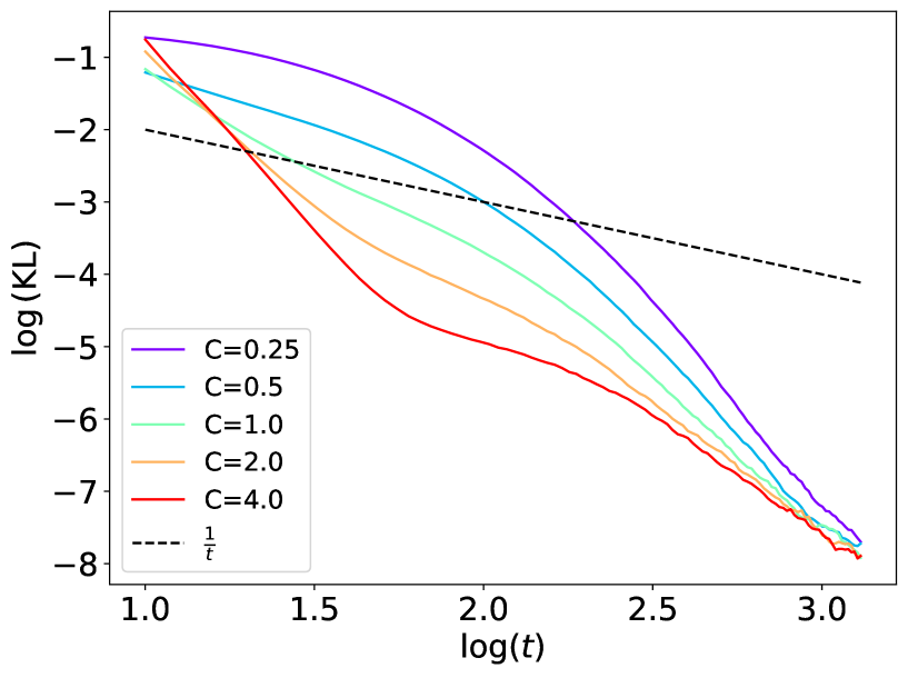
(a) $V(x)=\frac{(x-1)^{2}}{8}$

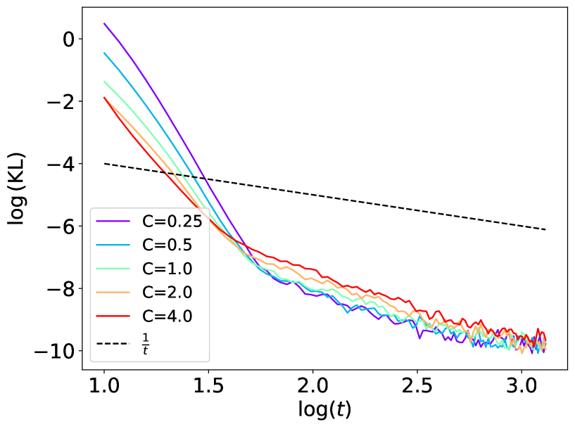
(b) $V(x)=\frac{(x+1)^{2}}{2}-\frac{\cos(x)}{2}$

Figure 1. Convergence rate of two strongly convex functions in one-dimension. Here y-axis represents the logarithm of the KL divergence between the empirical distribution and the invariant measure $\pi(t,x)$ given by (31). And the x-axis is $\log(t)$. We have also added a dotted line representing $t^{-1}$ on a logarithmic scale for comparison.

We consider $V:\mathbb{R}^{d}\to\mathbb{R}$, $d=1,2$, and $\beta(t)=\frac{C}{\log(t)}$ for some choices of constant $C$. We would like to compare the KL divergence between the invariant measure $\pi(t,x)$ given by (31) and the sample distribution of $X_{t}$ that follows (35) for different choices of $V(x)$ and $\beta(t)$. We first sample $M=10^{6}$ particles from $\mathcal{N}(0,1)$. Then we evolve (35) using the Euler-Maruyama scheme shown below for $N=10000$ steps with a step size of $h=0.002$:

$$X_{n+1}=X_{n}-h\nabla V(X_{n})+\sqrt{\frac{2C}{\log(nh+t_{0})}}B_{n}\,,$$ (39)

where $B_{n}\sim\mathcal{N}(0,\sqrt{h})$, and $t_{0}=e$. During each iteration, we compute the discrete KL divergence between the empirical distribution of the $M$ particles and the invariant measure $\pi(t,x)$ given by (31). The KL divergence between two discrete distributions is given by $\mathrm{D}_{\mathrm{KL}}(p\|q)=\sum p_{i}\log(p_{i}/q_{i})$. At each iteration, we can use the histogram of the empirical distribution to get $p_{i}$ for $i=1,...,K$. Here $K$ is the number of bins of the histogram and we choose $K=50$ in our numerical experiment. Let $x_{i}$ denote the location (midpoint between the left and right bin edge) of each of the bins. Then at the $n$-th iteration, we can compute $q_{i}=\frac{1}{Z}\exp(-\frac{V(x_{i})}{\beta(nh+t_{0})})$, where $Z=\int_{\mathbb{R}}\exp(-\frac{V(x)}{\beta(nh+t_{0})})dx$ is the normalization constant and can be estimated numerically. The results are plotted (on a logarithmic scale) in Fig. 1 for strongly convex $V(x)$ and Fig. 2 for non-convex function $V(x)$ with different constant $C$ in the expression of $\beta(t)$.

In the strongly-convex setting (Fig. 1), we see that the KL divergence between empirical distribution and $\pi$ decreases at a rate faster than $O(1/t)$ for all choices of $C$. In the non-convex setting (Fig. 2), we observe a convergence rate faster than $O(1/t)$ at the beginning which then drops to $O(1/t)$ as $t$ becomes larger. In two-dimension (Fig. 3), we observe the $O(1/t)$ convergence in both the strongly convex examples (3(a) and 3(b)) and the non-convex example (3(c)). In our two-dimensional examples, we used $M=10^{6}$ particles, $N=10000$ steps with a stepsize of $h=0.001$. We have 50 bins in both $x$ and $y$ direction which gives a total of $2500$ bins.

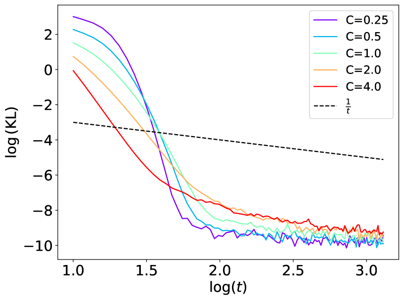
(a) $V(x)=\frac{(x+2)^{4}}{4}-\frac{x^{2}}{2}+\frac{x}{8}$

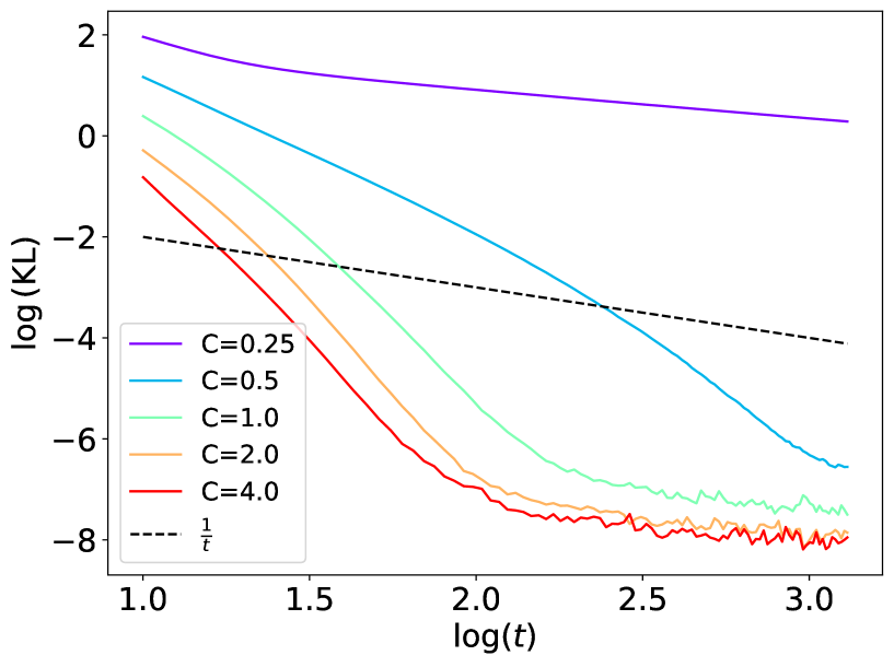
(b) $V(x)=\frac{(x-2)^{2}}{2}-\frac{\sin(5x)}{2}$

Figure 2. Convergence rate of two non-convex functions in one-dimension.

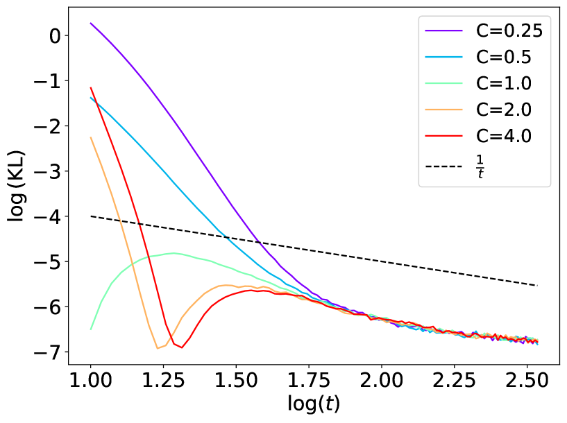
(a) $\frac{x^{2}+y^{2}}{2}$

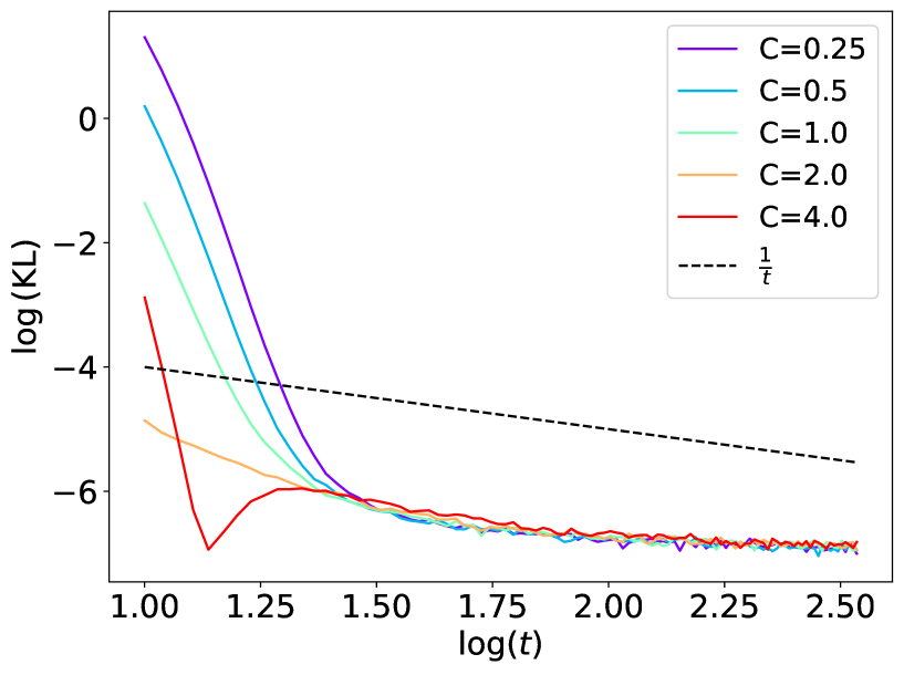
(b) $x^{2}+y^{2}-\frac{\cos(x+y)}{2}$

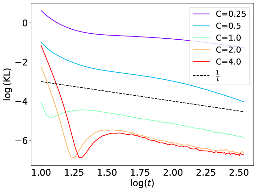
(c) $x^{2}+y^{2}-\sin(2x+2y)$

Figure 3. Convergence rate of two strongly convex functions (A) and (B), and a non-convex function (C) in two dimensions.

5. Example II: non-degenerate, non-reversible SDEs

In this section, we apply Theorem 2 to study the following non-degenerate and non-reversible SDE,

$$\begin{split}dX_{t}=&\Big{(}-\alpha(t,X_{t})\alpha(t,X_{t})^{\mathsf{T}}\nabla V(X_{t})+\beta(t)\nabla\cdot\Big{(}\alpha(t,X_{t})\alpha(t,X_{t})^{\mathsf{T}}\Big{)}-\gamma(t,X_{t})\Big{)}dt\\ &+\sqrt{2\beta(t)}\alpha(t,X_{t})dB_{t}.\end{split}$$ (40)

Again, we have $d=n$, $m=0$. The above SDE is a variant of SDE (30) by adding a smooth irreversible vector field $\gamma(t,x)\in{\mathbb{R}}^{d}$, which is assumed to satisfy

$$\nabla\cdot(e^{-V(x)}\gamma(t,x))=0.$$

In the current setting, we focus on a special case with $a(t,x)=\sqrt{\beta(t)}\alpha(t,x)$. In particular, we consider the diffusion matrix $a$ in a special form, which satisfies $a_{ii}(t,x)=a_{ii}(t,x_{i})=\sqrt{\beta(t)}\alpha_{ii}(x_{i})>0$, for all $x_{i}\in\mathbb{R}$, $i=1,\cdots,n$, with

$$\alpha(x)=\begin{pmatrix}\alpha_{11}(x_{1})&0&\cdots&0\\ 0&\alpha_{22}(x_{2})&\cdots&0\\ 0&0&\cdots&0\\ 0&\cdots&0&\alpha_{nn}(x_{n})\end{pmatrix}.$$ (41)

Proposition 6.

The Hessian matrix $\mathfrak{R}$ for the above time-dependent non-reversible SDE has the following form,

$$\mathfrak{R}-\frac{1}{2}\partial_{t}(aa^{\mathsf{T}})=\mathfrak{R}_{a}+\mathfrak{R}_{\gamma_{a}}-\frac{1}{2}\partial_{t}(aa^{\mathsf{T}}),$$

where

$$\begin{cases}\mathfrak{R}_{a,ii}&=\beta(t)\alpha_{ii}^{3}\partial_{x_{i}}\alpha_{ii}\partial_{x_{i}}V(x)+\beta(t)\alpha_{ii}^{4}\partial^{2}_{x_{i}x_{i}}V(x)-\beta^{2}(t)\alpha_{ii}^{3}\partial_{x_{i}x_{i}}^{2}\alpha_{ii},\quad\hfill i=1,\cdots,n;\\ \mathfrak{R}_{a,ij}&=\beta(t)\alpha_{ii}^{2}\alpha_{jj}^{2}\partial^{2}_{x_{i}x_{j}}V(x),\hfill i,j=1,\cdots,n,i\neq j;\\ \mathfrak{R}_{\gamma_{a},ii}&=\beta(t)\gamma_{i}\alpha_{ii}\partial_{x_{i}}\alpha_{ii}-\beta(t)\partial_{x_{i}}\gamma_{i}(\alpha_{ii})^{2},\hfill i=1,\cdots,n;\\ \mathfrak{R}_{\gamma_{a},ij}&=-\frac{1}{2}\beta(t)[\partial_{x_{i}}\gamma_{j}(\alpha_{jj})^{2}+\partial_{x_{j}}\gamma_{i}(\alpha_{ii})^{2}],\hfill i,j=1,\cdots,n,i\neq j.\end{cases}$$ (42)

Proof  Following [13][Proposition 2], we have

$$\begin{cases}\mathfrak{R}_{a,ii}&=-a_{ii}^{3}\partial_{x_{i}}a_{ii}\partial_{x_{i}}\log\pi-a_{ii}^{4}\partial^{2}_{x_{i}x_{i}}\log\pi-a_{ii}^{3}\partial_{x_{i}x_{i}}^{2}a_{ii},\hfill i=1,\cdots,n;\\ \mathfrak{R}_{a,ij}&=-a_{ii}^{2}a_{jj}^{2}\partial^{2}_{x_{i}x_{j}}\log\pi,\hfill i,j=1,\cdots,n,i\neq j.\\ \mathfrak{R}_{\gamma_{a},ii}&=\gamma_{i}a_{ii}\partial_{x_{i}}a_{ii}-\partial_{x_{i}}\gamma_{i}(a_{ii})^{2},\hfill i=1,\cdots,n;\\ \mathfrak{R}_{\gamma_{a},ij}&=-\frac{1}{2}[\partial_{x_{i}}\gamma_{j}(a_{jj})^{2}+\partial_{x_{j}}\gamma_{i}(a_{ii})^{2}],\hfill i,j=1,\cdots,n,i\neq j.\end{cases}$$

Plugging in the matrix $a(t,x)=\sqrt{\beta(t)}\alpha(x)$, we derive the desired matrix $\mathfrak{R}$.   As in the previous section, if there exists a constant $\lambda>0$, such that

$$\mathfrak{R}-\frac{1}{2}\partial_{t}(aa^{\mathsf{T}})\succeq\lambda aa^{\mathsf{T}},$$

then the Fisher information decay in Theorem 2 holds.

5.1. Time dependent non-reversible Langevin dynamics

In this section, we consider a special case with $n=2$, $\alpha\equiv\mathbb{I}$, and $\gamma=\frac{1}{\beta(t)}\mathsf{J}\nabla V$, where the matrix $\mathsf{J}$ has the following form, for some smooth function $c(t):\mathbb{R}^{+}\rightarrow\mathbb{R}$

$$\mathsf{J}=\begin{pmatrix}0&\beta(t)c(t)\\ -\beta(t)c(t)&0\end{pmatrix},\quad i.e.\quad\gamma(t,x)=\begin{pmatrix}c(t)\partial_{x_{2}}V(x)\\ -c(t)\partial_{x_{1}}V(x)\end{pmatrix}.$$

It is easy to check that $\nabla\cdot(\pi(t,x)\gamma(t,x))=0$ (e.g.: see (45) below). Applying Proposition 6, we have

$$\mathfrak{R} = \beta(t)\begin{pmatrix}\partial_{x_{1}x_{1}}V-c(t)\partial_{x_{1}x_{2}}V&\partial_{x_{1}x_{2}}V-c(t)\frac{1}{2}(-\partial_{x_{1}x_{1}}V+\partial_{x_{2}x_{2}}V)\\ \partial_{x_{2}x_{1}}V-c(t)\frac{1}{2}(-\partial_{x_{1}x_{1}}V+\partial_{x_{2}x_{2}}V)&\partial_{x_{2}x_{2}}V+c(t)\partial_{x_{2}x_{1}}V\end{pmatrix}$$ (43)

$$=: \beta(t)\mathsf{B}(t,x).$$

Comparing with the Corollary 9 and Corollary 10, the irreversible vector field $\gamma(t,x)$ only changes the matrix $\mathfrak{R}$, but does not change the estimate of $\mathrm{A}(t)$. If the smallest eigenvalue of $\mathsf{B}(t,x)$ is bigger than the smallest eigenvalue of $\nabla^{2}_{xx}V$ for a proper choice of the function $c(t)$, the convergence of stochastic dynamics (40) can be faster than the underdamped Langevin dynamics (30).

Variable matrices $\mathsf{J}$. We also study a case with the variable coefficient anti-symmetric vector field. Consider a two-dimensional stochastic differential equation:

$$dX_{t}=(-\nabla V(X_{t})-\mathsf{J}(t,X_{t})\nabla V(X_{t})-\beta(t)\nabla\cdot\mathsf{J}(t,X_{t}))dt+\sqrt{2\beta(t)}dB_{t},$$ (44)

where we define

$$\mathsf{J}=\begin{pmatrix}0&c(t,x)\\ -c(t,x)&0\end{pmatrix},$$

and

$$\gamma(t,x) = aa^{\mathsf{T}}\nabla\log\pi-b+\beta(t)(\frac{\partial}{\partial x_{j}}(\alpha\alpha^{\mathsf{T}})_{ij})_{i=1}^{n}$$

$$= \begin{pmatrix}c(t,x)\partial_{x_{2}}V(x)\\ -c(t,x)\partial_{x_{1}}V(x)\end{pmatrix}+\beta(t)\begin{pmatrix}-\partial_{x_{2}}c(t,x)\\ \partial_{x_{1}}c(t,x)\end{pmatrix}.$$

Here $\pi(t,x)=\frac{1}{Z(t)}e^{-\frac{V(x)}{\beta(t)}}$. We also have the fact that $\nabla\cdot(\pi\gamma)=\frac{1}{Z}\nabla\cdot(e^{-V}\gamma)=0$, since

$$\nabla\cdot(\pi\gamma) = \nabla\cdot\Big{(}\pi\begin{pmatrix}c(t,x)\partial_{x_{2}}V(x)\\ -c(t,x)\partial_{x_{1}}V(x)\end{pmatrix}+\pi\beta\begin{pmatrix}-\partial_{x_{2}}c(t,x)\\ \partial_{x_{1}}c(t,x)\end{pmatrix}\Big{)}$$ (45)

$$= \langle\nabla\pi,\begin{pmatrix}c(t,x)\partial_{x_{2}}V(x)\\ -c(t,x)\partial_{x_{1}}V(x)\end{pmatrix}+\beta\begin{pmatrix}-\partial_{x_{2}}c(t,x)\\ \partial_{x_{1}}c(t,x)\end{pmatrix}\rangle$$

$$+\pi\nabla\cdot\Big{(}\begin{pmatrix}c(t,x)\partial_{x_{2}}V(x)\\ -c(t,x)\partial_{x_{1}}V(x)\end{pmatrix}+\beta\begin{pmatrix}-\partial_{x_{2}}c(t,x)\\ \partial_{x_{1}}c(t,x)\end{pmatrix}\Big{)}$$

$$= -\frac{\pi}{\beta}\Big{\langle}\begin{pmatrix}\partial_{x_{1}}V\\ \partial_{x_{2}}V\end{pmatrix},\begin{pmatrix}c(t,x)\partial_{x_{2}}V(x)\\ -c(t,x)\partial_{x_{1}}V(x)\end{pmatrix}+\beta\begin{pmatrix}-\partial_{x_{2}}c(t,x)\\ \partial_{x_{1}}c(t,x)\end{pmatrix}\Big{\rangle}$$

$$+\pi\partial_{x_{1}}[c(t,x)\partial_{x_{2}}V-\beta\partial_{x_{2}}c(t,x)]+\pi\partial_{x_{2}}[-c(t,x)\partial_{x_{1}}V+\beta\partial_{x_{1}}c(t,x)]$$

$$= -\frac{\pi}{\beta}(c\partial_{x_{1}}V\partial_{x_{2}}V-c\partial_{x_{1}}V\partial_{x_{2}}V)+\pi(\partial_{x_{1}}V\partial_{x_{2}}c-\partial_{x_{2}}V\partial_{x_{1}}c)$$

$$+\pi[\partial_{x_{1}}c\partial_{x_{2}}V+c\partial_{x_{1}x_{2}}V-\beta\partial_{x_{1}x_{2}}c-\partial_{x_{2}}c\partial_{x_{1}}V-c\partial_{x_{1}x_{2}}V+\beta\partial_{x_{1}x_{2}}c]$$

$$=0.$$

For the matrix $\mathfrak{R}$, with $\gamma_{1}=c(t,x)\partial_{x_{2}}V-\beta(t)\partial_{x_{2}}c(t,x)$, and $\gamma_{2}=-c(t,x)\partial_{x_{1}}V+\beta(t)\partial_{x_{1}}c(t,x)$, we have

$$\mathfrak{R}= \beta\begin{pmatrix}\partial_{x_{1}x_{1}}V&\partial_{x_{1}x_{2}}V\\ \partial_{x_{2}x_{1}}V&\partial_{x_{2}x_{2}}V\end{pmatrix}-\beta\begin{pmatrix}\partial_{x_{1}}\gamma_{1}&\frac{1}{2}(\partial_{x_{1}}\gamma_{2}+\partial_{x_{2}}\gamma_{1})\\ \frac{1}{2}(\partial_{x_{1}}\gamma_{2}+\partial_{x_{2}}\gamma_{1})&\partial_{x_{2}}\gamma_{2}\end{pmatrix}$$

$$= \quad\beta\begin{pmatrix}\partial_{x_{1}x_{1}}V&\partial_{x_{1}x_{2}}V\\ \partial_{x_{2}x_{1}}V&\partial_{x_{2}x_{2}}V\end{pmatrix}$$

$$-\beta\begin{pmatrix}\partial_{x_{1}}c\partial_{x_{2}}V+c\partial_{x_{1}x_{2}}V-\beta\partial_{x_{1}x_{2}}c&\mathfrak{R}_{\gamma,12}\\ \mathfrak{R}_{\gamma,12}&-\partial_{x_{2}}c\partial_{x_{1}}V-c\partial_{x_{2}x_{1}}V+\beta\partial_{x_{2}x_{1}}c\end{pmatrix},$$

where $\mathfrak{R}_{\gamma,12}=\frac{1}{2}[c(\partial_{x_{2}x_{2}}V-\partial_{x_{1}x_{1}}V)+\beta(-\partial_{x_{2}x_{2}}c+\partial_{x_{1}x_{1}}c)+\partial_{x_{2}}c\partial_{x_{2}}V-\partial_{x_{1}}c\partial_{x_{1}}V]$.

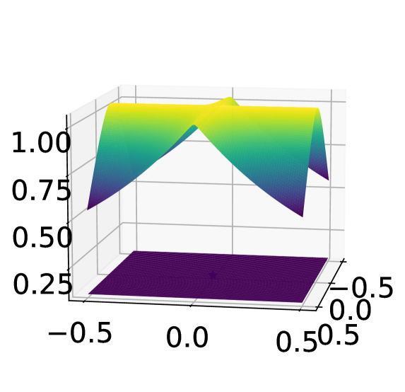
Figure 4. Eigenvalue comparison between $V(x)$ and $\mathfrak{R}(x)$ for $x\in[-0.5,0.5]\times[-0.5,0.5]$. The parameters are chosen as in Example 1. The yellow surface represents the smallest eigenvalue of $\mathfrak{R}(x)$ and the purple surface represents the smallest eigenvalue of $V(x)$. The global minimum of $V$ is marked with a blue asterisk. As shown in the figure, the smallest eigenvalue of $\mathfrak{R}$ is larger than that of $V$ near the global minimum.

Example 1.

Let us consider an example where $V$ is a two dimensional quadratic form with

$$\nabla_{xx}^{2}V=\begin{pmatrix}a&0\\ 0&b\end{pmatrix},$$

such that $a>b>0$. This implies that $\nabla_{xx}^{2}V$ is positive definite. We assume that the minimum of V is at $(0,0)$. Let $c(t,x)=c(x)$ be another quadratic form such that it has the same global minimum as $V$. Denote by $c^{\prime\prime}_{ij}=\partial_{x_{i}x_{j}}c$. We now consider the neighbourhood near the global minimum, so that all first-order partial derivatives of $V$ can be neglected, and $c\approx 0$. Then the matrix $\mathfrak{R}$ is approximated by

$$\mathfrak{R}\approx\beta\begin{pmatrix}a+\beta c^{\prime\prime}_{12}&-\frac{1}{2}\beta(c^{\prime\prime}_{11}-c^{\prime\prime}_{22})\\ -\frac{1}{2}\beta(c^{\prime\prime}_{11}-c^{\prime\prime}_{22})&b-\beta c^{\prime\prime}_{12}\end{pmatrix}\,.$$

There are many choices of $c$ to make the smallest eigenvalues of $\mathfrak{R}$ larger than that of $V$. For instance, take $c^{\prime\prime}_{11}=c^{\prime\prime}_{22}=0$, $c^{\prime\prime}_{12}=(b-a)/2\beta(t)$. In this case, the smallest eigenvalue is $(a+b)/2$ whereas the smallest eigenvalue of $V$ is $b$. A visualization is shown Fig. 4 when $a=2$, $b=0.1$, $\beta=1$. Now let us consider $\beta(t)=\frac{1}{t_{0}+t}$ for $t_{0}=1$. We use the Euler-Maruyama scheme to run (35) and (44) with a step size of $dt=5\times 10^{-5}$ for $3*10^{5}$ iterations. We use $10^{4}$ particles initially sampled from a standard Gaussian distribution for our comparison. The result is demonstrated in Fig. 5. We observe that equation (44) yields a faster convergence towards the global minimum than equation (35).

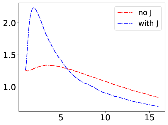
Figure 5. Convergence comparison between (35) and (44) in Example 1. $x$-axis represents time. $y$-axis represents the average distance of the particles to the global minimum using the two SDEs.

6. Example III: underdamped Langevin dynamics

In this section, we consider an underdamped Langevin dynamics with variable diffusion coefficients:

$$\left\{\begin{aligned} dx_{t}=&v_{t}dt\\ dv_{t}=&(-r(t,x_{t})v_{t}-\nabla_{x}V(x_{t}))dt+\sqrt{2r(t,x_{t})}dB_{t},\end{aligned}\right.$$ (46)

where $n=m=1$, $d=n+m=2$, $X_{t}=(x_{t},v_{t})\in\mathbb{R}^{2}$ is a two dimensional stochastic process, $V\in\mathbb{C}^{2}(\mathbb{R}^{1})$ is a Lipschitz potential function with assumption $\int_{\mathbb{R}^{1}}e^{-V(x)}dx<+\infty$, $B_{t}$ is a standard Brownian motion in $\mathbb{R}$, and $r:\mathbb{R}_{+}\times\mathbb{R}^{2}\rightarrow\mathbb{R}_{+}$ is a positive smooth Lipschitz function. Indeed, the reference measure $\pi(t,x,v)=\pi(x,v)$ is the invariant measure, defined as

$$\pi(x,v)=\frac{1}{Z}e^{-H(x,v)},\quad H(x,v)=\frac{v^{2}}{2}+V(x),$$

where $Z=\int_{\mathbb{R}^{2}}e^{-H(x,v)}dxdv<+\infty$ is a normalization constant. Following the definition of diffusion matrix $a$, the vector field $\gamma$ and the correction term $\mathcal{R}$, we have

$$a=\begin{pmatrix}0\\ \sqrt{r(t,x)}\end{pmatrix},\quad\gamma=\begin{pmatrix}-v\\ \nabla V(x)\end{pmatrix},\quad\text{and}\quad\mathcal{R}(t,x,\pi)=0,$$ (47)

since $\partial_{t}\pi(x,v)=0$, and $\nabla\cdot(\pi\gamma)=0$.

Consider a time-dependent vector field $z=\begin{pmatrix}z_{1}(t,x)\\ z_{2}(t,x)\end{pmatrix}$. We have the following proposition. The derivation follows similar studies in the time-independent case as shown in [13]. We skip the details here.

Proposition 7.

For the time-dependent underdamped Langevin dynamics, the time-dependent Hessian matrix function $\mathfrak{R}(t,x):\mathbb{R}_{+}\times\mathbb{R}^{2}\rightarrow\mathbb{R}^{2\times 2}$ has the following form,

$$\mathfrak{R} = \mathfrak{R}_{a}+\mathfrak{R}_{z}+\mathfrak{R}_{\pi}-\mathfrak{M}_{\Lambda}+\mathfrak{R}_{\gamma_{a}}+\mathfrak{R}_{\gamma_{z}},$$

where $a_{21}=\sqrt{r}$, and

$$\mathfrak{R}_{a} = \begin{pmatrix}0&0\\ 0&-\frac{\partial^{2}\log\pi}{\partial v^{2}}|a_{21}|^{4}\end{pmatrix},\quad\mathfrak{R}_{\pi}=\begin{pmatrix}0&0\\ 0&C_{\pi}\end{pmatrix},$$

$$\mathfrak{R}_{z} = \frac{1}{2}\Big{[}\begin{pmatrix}0\\ -z^{\mathsf{T}}_{1}\nabla((a_{21})^{2}\frac{\partial\log\pi}{\partial v})\end{pmatrix}z^{\mathsf{T}}_{1}+z_{1}\begin{pmatrix}0&-z^{\mathsf{T}}_{1}\nabla((a_{21})^{2}\frac{\partial\log\pi}{\partial v})\end{pmatrix}\Big{]},$$

$$\mathfrak{R}_{\gamma_{a}} = {\frac{1}{2}}\gamma_{1}\nabla_{1}(aa^{\mathsf{T}})-\frac{1}{2}\Big{[}(\nabla\gamma)^{\mathsf{T}}aa^{\mathsf{T}}+aa^{\mathsf{T}}\nabla\gamma\Big{]},$$

$$\mathfrak{R}_{\gamma_{z}} = {\frac{1}{2}}\gamma_{1}\nabla_{1}(zz^{\mathsf{T}})-\frac{1}{2}\Big{[}(\nabla\gamma)^{\mathsf{T}}zz^{\mathsf{T}}+zz^{\mathsf{T}}\nabla\gamma\Big{]},\quad\mathfrak{M}_{\Lambda}=\frac{1}{(a_{21})^{2}}\mathsf{K}^{\mathsf{T}}(aa^{\mathsf{T}}+zz^{\mathsf{T}})^{-1}\mathsf{K},$$

with

$$C_{\pi} = 2\Big{[}z^{\mathsf{T}}_{1}z^{\mathsf{T}}_{1}\nabla^{2}a_{21}a_{21}+(z^{\mathsf{T}}_{1}\nabla a_{21})^{2}+(z^{\mathsf{T}}_{1}\nabla\log\pi)[z^{\mathsf{T}}_{1}\nabla a_{21}a_{21}]\Big{]},$$

$$\mathsf{K} = \begin{pmatrix}\mathsf{0}&2z_{1}^{2}\partial_{x}[a_{21}]a_{21}-\frac{1}{2}\beta\gamma_{1}(a_{21})^{2}\\ -z_{1}^{2}\partial_{x}[a_{21}]a_{21}+\frac{1}{2}\beta\gamma_{1}(a_{21})^{2}&z_{1}z_{2}\partial_{x}[a_{21}]a_{21}\end{pmatrix}.$$

If there exists a constant $\lambda>0$, such that

$$\mathfrak{R}-\frac{1}{2}\partial_{t}(aa^{\mathsf{T}}+zz^{\mathsf{T}})\succeq\lambda(aa^{\mathsf{T}}+zz^{\mathsf{T}}),$$

then the Fisher information decay in Theorem 2 holds.

In the following, we consider a special case where we choose $r(t,x)=r(t)$, and $z=\begin{pmatrix}z_{1}\\ z_{2}\end{pmatrix}$, for some constants $z_{1},z_{2}\in\mathbb{R}$. In this case, the matrix $\mathfrak{R}(t,x)$ is simplified into the following form,

$$\mathfrak{R}=\mathfrak{R}_{a}+\mathfrak{R}_{z}+\mathfrak{R}_{\gamma_{a}}+\mathfrak{R}_{\gamma_{z}},$$

where we have

$$\mathfrak{R}_{a} = \begin{pmatrix}0&0\\ 0&(r(t))^{2}\end{pmatrix},\quad\mathfrak{R}_{z}=r(t)\begin{pmatrix}0&\frac{z_{1}z_{2}}{2}\\ \frac{z_{1}z_{2}}{2}&z_{2}^{2}\end{pmatrix},$$

$$\mathfrak{R}_{\gamma_{a}} = r(t)\begin{pmatrix}0&\frac{1}{2}\\ \frac{1}{2}&0\end{pmatrix},\quad\mathfrak{R}_{\gamma_{z}}=\begin{pmatrix}z_{1}z_{2}&\frac{1}{2}(z_{2}^{2}-z_{1}^{2}\nabla_{xx}^{2}V)\\ \frac{1}{2}(z_{2}^{2}-z_{1}^{2}\nabla_{xx}^{2}V)&-z_{1}z_{2}\nabla^{2}_{xx}V\end{pmatrix}.$$

Proposition 8 (Sufficient conditions).

In the above example,

$$\mathfrak{R}-\frac{1}{2}\partial_{t}(aa^{\mathsf{T}})$$

$$= \begin{pmatrix}z_{1}z_{2}&\frac{1}{2}[r(t)+r(t)z_{1}z_{2}+z_{2}^{2}-z_{1}^{2}\nabla^{2}_{xx}V(x)]\\ \frac{1}{2}[r(t)+r(t)z_{1}z_{2}+z_{2}^{2}-z_{1}^{2}\nabla^{2}_{xx}V(x)]&(r(t))^{2}+r(t)z_{2}^{2}-z_{1}z_{2}\nabla^{2}_{xx}V(x)-\frac{1}{2}\partial_{t}r(t)\end{pmatrix}.$$

Assume that $0<\underline{\lambda}\leq\partial_{xx}^{2}V\leq\overline{\lambda}$, and there exist constants $z_{2}\in(0,\frac{r(t)+\sqrt{r(t)^{2}+4r(t)}}{2})$, for all $t\geq t_{0}$, such that $\underline{\lambda}$, $\overline{\lambda}$ satisfy the following conditions:

$$-\overline{\lambda}^{2}+[2(r(1+z_{2})-z_{2}^{2})]\underline{\lambda}-[(1-z_{2})r+z_{2}^{2}]^{2}-2z_{2}\partial_{t}r>0,\quad r^{2}+rz_{2}^{2}-\overline{\lambda}z_{2}-\frac{1}{2}\partial_{t}r>0.$$ (48)

Then there exists a function $\lambda(t)>0$, for $t>t_{0}$, such that

$$\mathfrak{R}-\frac{1}{2}\partial_{t}(aa^{\mathsf{T}})\succeq\lambda(aa^{\mathsf{T}}+zz^{\mathsf{T}}).$$ (49)

Proof  For notation convenience, we take $r=r(t)$. It is sufficient to prove $\mathsf{det}(\mathfrak{R})>0$ for $z_{1}z_{2}>0$ and $r^{2}+rz_{2}^{2}-\partial^{2}_{xx}Vz_{1}z_{2}-\frac{1}{2}\partial_{t}r>0$, which is equivalent to

$$z_{1}z_{2}(r^{2}+rz_{2}^{2}-\partial^{2}_{xx}Vz_{1}z_{2}-\frac{1}{2}\partial_{t}r)-\frac{1}{4}(rz_{1}z_{2}+z_{2}^{2}-\partial^{2}_{xx}Vz_{1}^{2}+r)^{2}>0.$$

It is equivalent to the following inequality:

$$-z_{1}^{4}(\partial_{xx}^{2}V)^{2}+[2(r(1+z_{1}z_{2})-z_{2}^{2})z_{1}^{2}]\partial_{xx}^{2}V-[(1-z_{1}z_{2})r+z_{2}^{2}]^{2}-2z_{1}z_{2}\partial_{t}r>0.$$ (50)

According to the assumption of $\partial_{xx}^{2}V$, it is sufficient to prove the following conditions:

$$\begin{cases}&z_{1}z_{2}>0,\quad r^{2}+rz_{2}^{2}-\overline{\lambda}z_{1}z_{2}-\frac{1}{2}\partial_{t}r>0,\quad(r(1+z_{1}z_{2})-z_{2}^{2})>0;\\ &-z_{1}^{4}\overline{\lambda}^{2}+[2(r(1+z_{1}z_{2})-z_{2}^{2})z_{1}^{2}]\underline{\lambda}-[(1-z_{1}z_{2})r+z_{2}^{2}]^{2}-2z_{1}z_{2}\partial_{t}r>0.\end{cases}$$ (51)

Let $z_{1}=1$, then (48) is equivalent to (51). We complete the proof.   The next corollary estimates $\lambda$ in (49) under some specific choices of parameters.

Corollary 11.

If $z_{2}=z_{1}=1$, $\overline{\lambda}>\frac{1}{2\underline{\lambda}}+\frac{\underline{\lambda}}{2}+1$, $\beta\geq\overline{\lambda}/2$, we have $\mathfrak{R}-\frac{1}{2}\partial_{t}(aa^{\mathsf{T}})\succeq 0$ as $t\to\infty$. Suppose further that $\beta=\overline{\lambda}/2$, and $\overline{\lambda}\geq\underline{\lambda}+2$, then we have $\lambda=\mathcal{O}(\frac{2\underline{\lambda}}{\overline{\lambda}}-\frac{1}{\overline{\lambda}^{2}})$.

Proof  Since $r(t)=\beta+C/\log t$, we have that $r(t)\to\beta$ and $\partial_{t}r\to 0$ as $t\to\infty$. Denote by $u(x)=\partial_{xx}^{2}V(x)$ and let $\beta=\overline{\lambda}/2$. We directly compute

$$\mathsf{det}(\mathfrak{R}-\frac{1}{2}\partial_{t}(aa^{\mathsf{T}})) =\frac{\overline{\lambda}^{2}}{4}+\frac{\overline{\lambda}}{2}-u(x)-\frac{1}{4}(\overline{\lambda}+1-u(x))^{2}$$

$$=\frac{\overline{\lambda}u(x)}{2}-\frac{u(x)}{2}-\frac{u(x)^{2}}{4}-\frac{1}{4}\,,$$ (52)

which is a quadratic function in $u(x)$. One can check that since $0<\underline{\lambda}\leq u(x)\leq\overline{\lambda}$ for all $x$, we have $\mathsf{det}(\mathfrak{R}-\frac{1}{2}\partial_{t}(aa^{\mathsf{T}}))>0$ as long as

$$\overline{\lambda}>\max\{\frac{1}{2\underline{\lambda}}+\frac{\underline{\lambda}}{2}+1,1+\sqrt{2}\}=\frac{1}{2\underline{\lambda}}+\frac{\underline{\lambda}}{2}+1\,.$$

Now let $\beta=\frac{\overline{\lambda}}{2}$. We want to find the largest $\lambda$, such that

$$\mathfrak{R}-\frac{1}{2}\partial_{t}(aa^{\mathsf{T}})-\lambda(aa^{\mathsf{T}}+zz^{\mathsf{T}})=\begin{pmatrix}1-\lambda&\frac{1}{2}(\overline{\lambda}+1-u(x))-\lambda\\ \frac{1}{2}(\overline{\lambda}+1-u(x))-\lambda&\frac{\overline{\lambda}^{2}}{4}+\frac{\overline{\lambda}}{2}-u(x)-(1+\frac{\overline{\lambda}}{2})\lambda\end{pmatrix}\succeq 0,$$

as $t\to\infty$. This translates to

$$1-\lambda \geq 0$$ (53)

$$\frac{\overline{\lambda}^{2}}{4}+\frac{\overline{\lambda}}{2}-u(x)-(1+\frac{\overline{\lambda}}{2})\lambda \geq 0$$ (54)

$$-1+2(\overline{\lambda}-1)u(x)-u(x)^{2}-\overline{\lambda}(\overline{\lambda}-2\lambda)\lambda \geq 0$$ (55)

Define $f(u,\lambda)=-1+2(\overline{\lambda}-1)u(x)-u(x)^{2}-\overline{\lambda}(\overline{\lambda}-2\lambda)\lambda$. It is clear that when $\lambda$ is fixed, $f$ is quadratic in $u$ and peaks at $u=\overline{\lambda}-1$. We also have that by definition of $u(x)$, we have $\underline{\lambda}\leq u(x)\leq\overline{\lambda}$ for all $x$. Therefore,

$$\min_{u}f(u,\lambda)=\min\{f(\overline{\lambda},\lambda),f(\underline{\lambda},\lambda),f(\overline{\lambda}-1,\lambda)\}\,.$$

When $\overline{\lambda}\geq\underline{\lambda}+2$, the above implies $\min_{u}f(u,\lambda)=f(\underline{\lambda},\lambda)$. Thus (55) is satisfied as long as $f(\underline{\lambda},\lambda)\geq 0$. We would like to maximize $\lambda$ subject to the constraints $f(\underline{\lambda},\lambda)\geq 0$ together with (53) and (54). From $\eqref{condition2}$ we have that

$$\lambda\leq\frac{\overline{\lambda}}{2}-\frac{\underline{\lambda}}{1+\overline{\lambda}/2}\,.$$

Using our assumption $\overline{\lambda}\geq\underline{\lambda}+2$ we get that

$$\frac{\overline{\lambda}}{2}-\frac{\underline{\lambda}}{1+\overline{\lambda}/2}>1\,.$$

Therefore, (53) and (54) together imply $\lambda\leq 1$. Observe that $f(\underline{\lambda},\lambda)$ is a quadratic function of $\lambda$, which produces two roots. It is straightforward to check that the larger root of $f$ is greater than 1. Hence, we conclude that $\lambda$ cannot be larger than the smaller root of $f$. We have

$$\lambda_{\rm max} =\frac{\overline{\lambda}}{4}-\frac{1}{4}\sqrt{\frac{8}{\overline{\lambda}}+\overline{\lambda}^{2}+16\frac{\underline{\lambda}}{\overline{\lambda}}-16\underline{\lambda}+8\frac{\underline{\lambda}^{2}}{\overline{\lambda}}}$$ (56)

$$\approx\frac{\overline{\lambda}}{4}-\frac{1}{4}\sqrt{\frac{8}{\overline{\lambda}}+\overline{\lambda}^{2}-16\underline{\lambda}}$$

$$\approx\frac{2\underline{\lambda}}{\overline{\lambda}}-\frac{1}{\overline{\lambda}^{2}}\,,$$

where our approximation holds when $\underline{\lambda}/\overline{\lambda}\ll 1$.  

6.1. Numerics

We plot the convergence of (46) in Fig. 6 for strongly convex functions and in Fig. 7 for non-convex functions. We have also plotted the KL divergence for $x$ variable only in Fig. 8 and Fig. 9. We used the same experiment setting as described in Section 4. In all of our numerical experiments, we observe that the KL divergence converges to 0. Comparing Fig. 1 with Fig. 8, we observe that the convergence speed of the underdamped Langevin dynamics (46) has a greater dependence on the constant than overdamped Langevin dynamics (35) does (recall that there is a constant $C$ in $\beta(t)$ in (35) and a constant $\beta$ in $r(t)$ in (46)). If the constant is chosen appropriately, the underdamped Langevin dynamics could converge much faster to the invariant measure than the overdamped Langevin dynamics. In both Fig. 8 and Fig. 9, we observe oscillations of the error, which is a typical phenomenon in accelerated convex optimization methods [1, 2, 32]. Designing the optimal constant $\beta$ in $r(t)$ with fast convergence speed is a delicate issue that is left for future studies.

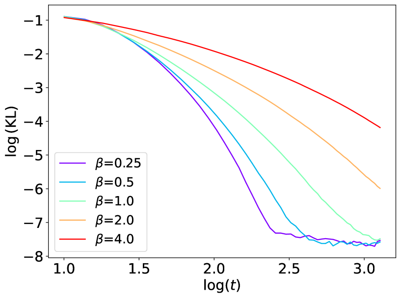
(a) $V(x)=\frac{(x-1)^{2}}{8}$

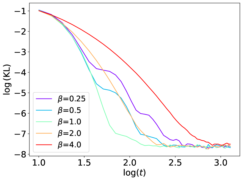
(b) $V(x)=\frac{(x+1)^{2}}{2}-\frac{\cos(x)}{2}$

Figure 6. Convergence rate of two strongly convex functions in one-dimension for (46) with $r(t)=\beta+1/\log(t)$, where we measure the KL divergence in both $x$ and $v$.

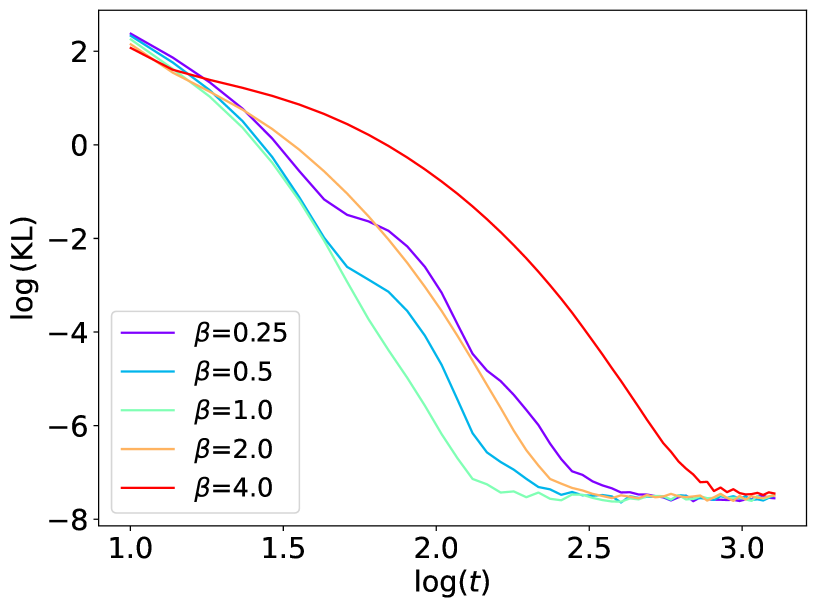
(a) $V(x)=\frac{(x+2)^{4}}{4}-\frac{x^{2}}{2}+\frac{x}{8}$

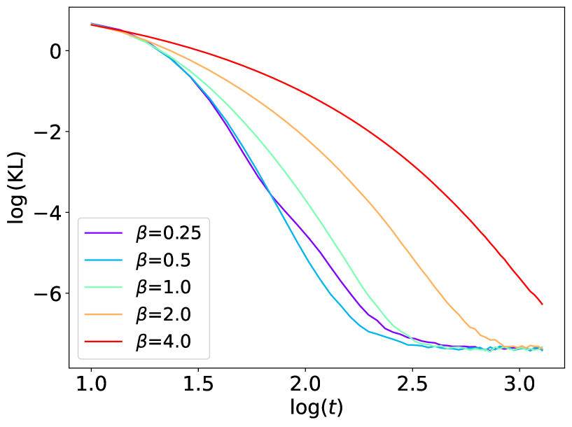
(b) $V(x)=\frac{(x-2)^{2}}{2}-\frac{\sin(5x)}{2}$

Figure 7. Convergence rate of two non-convex functions in one-dimension for (46) with $r(t)=\beta+1/\log(t)$, where we measure the KL divergence in both $x$ and $v$ variables.

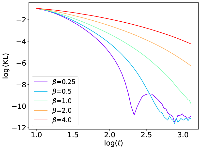
(a) $V(x)=\frac{(x-1)^{2}}{8}$

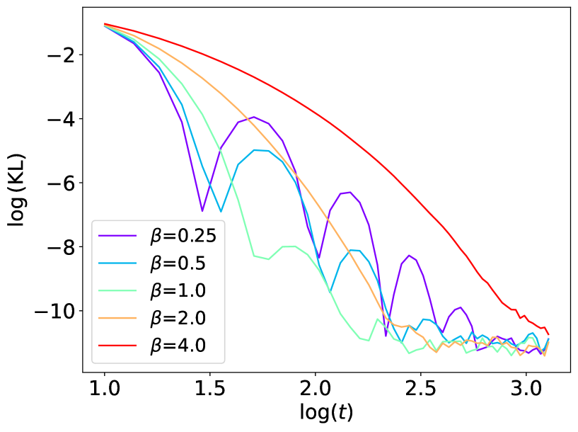
(b) $V(x)=\frac{(x+1)^{2}}{2}-\frac{\cos(x)}{2}$

Figure 8. Convergence rate of two strongly convex functions in one-dimension for (46), where we only measure the KL divergence in the $x$ variable.

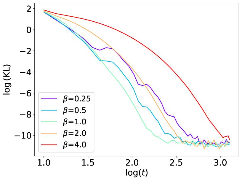
(a) $V(x)=\frac{(x+2)^{4}}{4}-\frac{x^{2}}{2}+\frac{x}{8}$

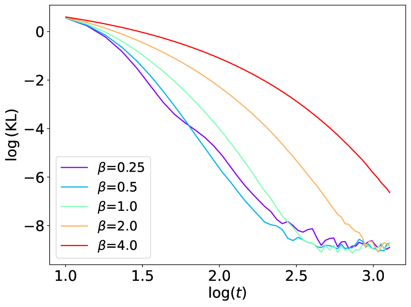
(b) $V(x)=\frac{(x-2)^{2}}{2}-\frac{\sin(5x)}{2}$

Figure 9. Convergence rate of two non-convex functions in one-dimension for (46), where we only measure the KL divergence in the $x$ variable.

7. Discussion

This paper studies the convergence analysis of time-dependent stochastic dynamics. We obtain a time-dependent Hessian matrix condition, which characterizes the convergence behavior of stochastic dynamics in terms of generalized Fisher information functionals. Examples of convergence speeds are shown, including over-damped, irreversible drift and degenerate diffusion, and underdamped Langevin dynamics. We also present several numerical experiments to verify the current convergence analysis of general stochastic dynamics.

In future work, we shall investigate the “optimal” choice of time-dependent matrix function $a$ and vector field $\gamma$ to find the global minimizer of a non-convex function $V$. Here, the “optimal” is in the sense of fast convergence speed towards the global minimizer. However, as we see in this paper, the convergence analysis for stochastic algorithms is more delicate than their deterministic counterparts. This requires us to estimate the general Hessian matrix, a.k.a. Ricci curvature lower bound, from both diffusion matrices $a$ and non-gradient vector from $\gamma$. They depend on the second derivatives of coefficients in stochastic dynamics. The other practical issue is the estimation of step sizes in the Euler-Maruyama scheme (39). The related discrete-time convergence analysis of stochastic algorithms is left in future studies.

Appendix

The time-independent version of the Hessian matrix is first introduced in [13][Definition 1]. For completeness of this paper, we introduce the time-dependent version of it for matrices $a(t,x)$ and $z(t,x)$, and we take the interpolation parameter $\beta=0$ for [13, Definition 1], since we do not always have $\nabla\cdot(\pi(t,x)\gamma(t,x))=0$, which can be seen in Lemma 4 and Lemma (6). This is a major difference compared to [13, Proposition 9].

Definition 3 (Hessian matrix).

Let matrices $a(t,x)$ and $z(t,x)$ satisfy the Hörmander like condtion, and conditions (7), (8). We define a bilinear form associated with SDE (1), and matrices $a,z$ as below, for a smooth vector field $\mathsf{U}\in C^{\infty}(\mathbb{R}^{n+m};\mathbb{R}^{n+m})$,

$$\mathfrak{R}(\mathsf{U},\mathsf{U}) = (\mathfrak{R}_{a}+\mathfrak{R}_{z}+\mathfrak{R}_{\pi}+\mathfrak{R}_{\gamma_{a}}+\mathfrak{R}_{\gamma_{z}})(\mathsf{U},\mathsf{U})-\Lambda_{1}^{\mathsf{T}}\Lambda_{1}-\Lambda_{2}^{\mathsf{T}}\Lambda_{2}+\mathsf{D}^{\mathsf{T}}\mathsf{D}+\mathsf{E}^{\mathsf{T}}\mathsf{E}.$$ (57)

We define $\mathfrak{R}(t,x):\mathbb{R}_{+}\times\mathbb{R}^{n+m}\rightarrow\mathbb{R}^{(n+m)\times(n+m)}$ as the corresponding time dependent matrix function such that

$$\mathsf{U}^{\mathsf{T}}\mathfrak{R}(x)\mathsf{U}=\mathfrak{R}(\mathsf{U},\mathsf{U}),$$ (58)

for all vector fields $\mathsf{U}$. The bilinear forms in (57) are defined as below.

$$\mathfrak{R}_{a}(\mathsf{U},\mathsf{U}) = \sum_{i,k=1}^{n}a^{\mathsf{T}}_{i}\nabla a^{\mathsf{T}}_{i}\nabla a^{\mathsf{T}}_{k}\mathsf{U}(a^{\mathsf{T}}_{k}\mathsf{U})+\sum_{i,k=1}^{n}a^{\mathsf{T}}_{i}a^{\mathsf{T}}_{i}\nabla^{2}a^{\mathsf{T}}_{k}\mathsf{U}(a^{\mathsf{T}}_{k}\mathsf{U})$$

$$-\sum_{i,k=1}^{n}a^{\mathsf{T}}_{k}\nabla a^{\mathsf{T}}_{i}\nabla a^{\mathsf{T}}_{i}\mathsf{U}(a_{k}^{\mathsf{T}}\mathsf{U})-\sum_{i,k=1}^{n}a^{\mathsf{T}}_{k}a^{\mathsf{T}}_{i}\nabla^{2}a^{\mathsf{T}}_{i}\mathsf{U}(a_{k}^{\mathsf{T}}\mathsf{U})$$

$$+\sum_{i=1}^{n}\sum_{\hat{k}=1}^{n+m}\Big{[}(aa^{\mathsf{T}}\nabla\log\pi)_{\hat{k}}\nabla_{\hat{k}}a^{\mathsf{T}}_{i}\mathsf{U}-a_{i}^{\mathsf{T}}\nabla(aa^{\mathsf{T}}\nabla\log\pi)_{\hat{k}}\mathsf{U}_{\hat{k}}\Big{]}a^{\mathsf{T}}_{i}\mathsf{U}$$

$$+\nabla a\circ\Big{(}\sum_{k=1}^{n}\Big{[}a^{\mathsf{T}}\nabla a^{\mathsf{T}}_{k}\mathsf{U}-a^{\mathsf{T}}_{k}\nabla a^{\mathsf{T}}\mathsf{U})\Big{]}a^{\mathsf{T}}_{k}\mathsf{U}\Big{)}-\langle\left(a^{\mathsf{T}}\nabla^{2}a\circ(a^{\mathsf{T}}\mathsf{U})\right),a^{\mathsf{T}}\mathsf{U}\rangle_{\mathbb{R}^{n}},$$

$$\mathfrak{R}_{z}(\mathsf{U},\mathsf{U}) = \sum_{i=1}^{n}\sum_{k=1}^{m}a^{\mathsf{T}}_{i}\nabla a^{\mathsf{T}}_{i}\nabla z^{\mathsf{T}}_{k}\mathsf{U}(z^{\mathsf{T}}_{k}\mathsf{U})+\sum_{i,k=1}^{n}a^{\mathsf{T}}_{i}a^{\mathsf{T}}_{i}\nabla^{2}z^{\mathsf{T}}_{k}\mathsf{U}(z^{\mathsf{T}}_{k}\mathsf{U})$$

$$-\sum_{i=1}^{n}\sum_{k=1}^{m}z^{\mathsf{T}}_{k}\nabla a^{\mathsf{T}}_{i}\nabla a^{\mathsf{T}}_{i}\mathsf{U}(z_{k}^{\mathsf{T}}\mathsf{U})-\sum_{i,k=1}^{n}z^{\mathsf{T}}_{k}a^{\mathsf{T}}_{i}\nabla^{2}a^{\mathsf{T}}_{i}\mathsf{U}(z_{k}^{\mathsf{T}}\mathsf{U})$$

$$+\sum_{k=1}^{m}\sum_{\hat{k}=1}^{n+m}\Big{[}(aa^{\mathsf{T}}\nabla\log\pi)_{\hat{k}}\nabla_{\hat{k}}z^{\mathsf{T}}_{k}\mathsf{U}-z_{k}^{\mathsf{T}}\nabla(aa^{\mathsf{T}}\nabla\log\pi)_{\hat{k}}\mathsf{U}_{\hat{k}}\Big{]}z^{\mathsf{T}}_{k}\mathsf{U}$$

$$+\nabla a\circ\Big{(}\sum_{k=1}^{m}\Big{[}a^{\mathsf{T}}\nabla z^{\mathsf{T}}_{k}\mathsf{U}-z^{\mathsf{T}}_{k}\nabla a^{\mathsf{T}}\mathsf{U})\Big{]}z^{\mathsf{T}}_{k}\mathsf{U}\Big{)}-\langle\left(z^{\mathsf{T}}\nabla^{2}a\circ(a^{\mathsf{T}}\mathsf{U})\right),z^{\mathsf{T}}\mathsf{U}\rangle_{\mathbb{R}^{m}},$$

$$\mathfrak{R}_{\pi}(\mathsf{U},\mathsf{U}) = 2\sum_{k=1}^{m}\sum_{i=1}^{n}\left[\nabla z^{\mathsf{T}}_{k}z^{\mathsf{T}}_{k}\nabla a^{\mathsf{T}}_{i}\mathsf{U}a^{\mathsf{T}}_{i}\mathsf{U}+z^{\mathsf{T}}_{k}\nabla z^{\mathsf{T}}_{k}\nabla a^{\mathsf{T}}_{i}\mathsf{U}a^{\mathsf{T}}_{i}\mathsf{U}+z^{\mathsf{T}}_{k}z^{\mathsf{T}}_{k}\nabla^{2}a^{\mathsf{T}}_{i}\mathsf{U}a^{\mathsf{T}}_{i}\mathsf{U}\right]$$

$$+2\sum_{k=1}^{m}\sum_{i=1}^{n}\Big{[}(z^{\mathsf{T}}_{k}\nabla a^{\mathsf{T}}_{i}\mathsf{U})^{2}+(z^{\mathsf{T}}\nabla\log\pi)_{k}\left[z^{\mathsf{T}}_{k}\nabla a^{\mathsf{T}}_{i}\mathsf{U}a^{\mathsf{T}}_{i}\mathsf{U}\right]\Big{]}$$

$$-2\sum_{j=1}^{m}\sum_{l=1}^{n}\left[\nabla a^{\mathsf{T}}_{l}a^{\mathsf{T}}_{l}\nabla z^{\mathsf{T}}_{j}\mathsf{U}z^{\mathsf{T}}_{j}\mathsf{U}+a^{\mathsf{T}}_{l}\nabla a^{\mathsf{T}}_{l}\nabla z^{\mathsf{T}}_{j}\mathsf{U}z^{\mathsf{T}}_{j}\mathsf{U}+a^{\mathsf{T}}_{l}a^{\mathsf{T}}_{l}\nabla^{2}z^{\mathsf{T}}_{j}\mathsf{U}z^{\mathsf{T}}_{j}\mathsf{U}\right]$$

$$-2\sum_{j=1}^{m}\sum_{l=1}^{n}\left[(a^{\mathsf{T}}_{l}\nabla z^{\mathsf{T}}_{j}\mathsf{U})^{2}+(a^{\mathsf{T}}\nabla\log\pi)_{l}\Big{[}a^{\mathsf{T}}_{l}\nabla z^{\mathsf{T}}_{j}\mathsf{U}z^{\mathsf{T}}_{j}\mathsf{U}\Big{]}\right],$$

$$\mathfrak{R}_{\gamma_{a}}(\mathsf{U},\mathsf{U}) = \frac{1}{2}\sum_{\hat{k}=1}^{n+m}\gamma_{\hat{k}}\langle\mathsf{U},\nabla_{\hat{k}}(aa^{\mathsf{T}})\mathsf{U}\rangle-\langle\nabla\gamma\mathsf{U},aa^{\mathsf{T}}\mathsf{U}\rangle_{\mathbb{R}^{n+m}},$$

$$\mathfrak{R}_{\gamma_{z}}(\mathsf{U},\mathsf{U}) = \frac{1}{2}\sum_{\hat{k}=1}^{n+m}\gamma_{\hat{k}}\langle\mathsf{U},\nabla_{\hat{k}}(zz^{\mathsf{T}})\mathsf{U}\rangle-\langle\nabla\gamma\mathsf{U},zz^{\mathsf{T}}\mathsf{U}\rangle_{\mathbb{R}^{n+m}}.$$

We define vector functions $\mathsf{D}:\mathbb{R}^{n+m}\rightarrow\mathbb{R}^{n^{2}\times 1}$, and $\mathsf{E}:\mathbb{R}^{n+m}\rightarrow\mathbb{R}^{(n\times m)\times 1}$ as below,

$$\mathsf{D}_{ik}=\sum_{\hat{i},\hat{k}=1}^{n+m}a^{\mathsf{T}}_{i\hat{i}}\partial_{x_{\hat{i}}}a^{\mathsf{T}}_{k\hat{k}}\mathsf{U}_{\hat{k}},\quad\mathsf{E}_{ik}=\sum_{\hat{i},\hat{k}=1}^{n+m}a^{\mathsf{T}}_{i\hat{i}}\partial_{x_{\hat{i}}}z^{\mathsf{T}}_{k\hat{k}}\mathsf{U}_{\hat{k}}.$$ (59)

For $\beta\in\mathbb{R}$, the vector functions $\Lambda_{1}:\mathbb{R}^{n+m}\rightarrow\mathbb{R}^{n^{2}\times 1}$ and $\Lambda_{2}:\mathbb{R}^{n+m}\rightarrow\mathbb{R}^{(n\times m)\times 1}$ are defined as, for $i,l\in\{1,\cdots,n\}$,

$$(\Lambda_{1})_{il} = \sum_{k=1}^{n}[\sum_{i^{\prime}=1}^{n+m}a^{\mathsf{T}}_{ii^{\prime}}\lambda^{i^{\prime}k}_{l}-\sum_{k^{\prime}=1}^{n+m}a^{\mathsf{T}}_{kk^{\prime}}\lambda^{k^{\prime}i}_{l}]a^{\mathsf{T}}_{k}\mathsf{U}+\sum_{k=1}^{m}\Big{(}\sum_{i^{\prime}=1}^{n+m}a^{\mathsf{T}}_{ii^{\prime}}\omega^{i^{\prime}k}_{l}-\sum_{k^{\prime}=1}^{n+m}z^{\mathsf{T}}_{kk^{\prime}}\lambda^{k^{\prime}i}_{l}\Big{)}z^{\mathsf{T}}_{k}\mathsf{U}$$

$$-\sum_{k=1}^{m}\sum_{i^{\prime}=1}^{n+m}a^{\mathsf{T}}_{ii^{\prime}}\omega^{i^{\prime}k}_{l}z^{\mathsf{T}}_{k}\mathsf{U}-\frac{\beta}{2}\alpha_{l}(a^{\mathsf{T}}_{i}\mathsf{U})+\frac{\beta}{2}\langle\mathsf{U},\gamma\rangle\mathbf{1}_{\{i=l\}}+\mathsf{D}_{il},$$

and for $i\in\{1,\cdots,n\}$, $l\in\{1,\cdots,m\}$,

$$(\Lambda_{2})_{il} = \sum_{k=1}^{n}[\sum_{i^{\prime}=1}^{n+m}a^{\mathsf{T}}_{ii^{\prime}}\lambda^{i^{\prime}k}_{l+n}-\sum_{k^{\prime}=1}^{n+m}a^{\mathsf{T}}_{kk^{\prime}}\lambda^{k^{\prime}i}_{l+n}]a^{\mathsf{T}}_{k}\mathsf{U}+\sum_{k=1}^{m}\Big{(}\sum_{i^{\prime}=1}^{n+m}a^{\mathsf{T}}_{ii^{\prime}}\omega^{i^{\prime}k}_{l+n}-\sum_{k^{\prime}=1}^{n+m}z^{\mathsf{T}}_{kk^{\prime}}\lambda_{l+n}^{k^{\prime}i}\Big{)}z^{\mathsf{T}}_{k}\mathsf{U}$$

$$+\sum_{k=1}^{n}\sum_{k^{\prime}=1}^{n+m}z^{\mathsf{T}}_{lk^{\prime}}\lambda^{k^{\prime}k}_{i}a^{\mathsf{T}}_{k}\mathsf{U}+z^{\mathsf{T}}_{l}\nabla a^{\mathsf{T}}_{i}\mathsf{U}-\sum_{k=1}^{m}\sum_{i^{\prime}=1}^{n+m}a^{\mathsf{T}}_{ii^{\prime}}\omega^{i^{\prime}k}_{l+n}z^{\mathsf{T}}_{k}\mathsf{U}-a^{\mathsf{T}}_{i}\nabla z^{\mathsf{T}}_{l}\mathsf{U}-\frac{\beta}{2}\alpha_{l+n}(a^{\mathsf{T}}_{i}\mathsf{U})+\mathsf{E}_{il}.$$

For each indices $i,k,\hat{k}$, assume that there exist smooth functions $\lambda^{i^{\prime}k}_{l}$, $\omega^{i^{\prime}k}_{l}$ and $\alpha_{l}$ for $l=1,\cdots,n+m$,

$$\nabla_{i^{\prime}}a^{\mathsf{T}}_{k\hat{k}} = \sum_{l=1}^{n}\lambda^{i^{\prime}k}_{l}a^{\mathsf{T}}_{l\hat{k}}+\sum_{l=1}^{m}\lambda^{i^{\prime}k}_{l+n}z^{\mathsf{T}}_{l\hat{k}},\quad\nabla_{i^{\prime}}z^{\mathsf{T}}_{k\hat{k}}=\sum_{l=1}^{n}\omega^{i^{\prime}k}_{l}a^{\mathsf{T}}_{l\hat{k}}+\sum_{l=1}^{m}\omega^{i^{\prime}k}_{l+n}z^{\mathsf{T}}_{l\hat{k}},$$

and $\gamma_{\hat{k}}=\sum_{l=1}^{n}\alpha_{l}a^{\mathsf{T}}_{l\hat{k}}+\sum_{l=1}^{m}\alpha_{l+n}z^{\mathsf{T}}_{l\hat{k}}$. For a vector function $\gamma\in\mathbb{R}^{n+m}$, we define $\nabla\gamma\in\mathbb{R}^{(n+m)\times(n+m)}$ with $(\nabla\gamma)_{ij}=\nabla_{i}\gamma_{j}$.

References

- [1] H. Attouch, Z. Chbani, J. Fadili, and H. Riahi. First-order optimization algorithms via inertial systems with Hessian driven damping. Mathematical Programming, 1–43, 2020.
- [2] H. Attouch, Z. Chbani, J. Fadili, and H. Riahi. Convergence of iterates for first-order optimization algorithms with inertia and Hessian driven damping. Optimization, 1–40, 2021.
- [3] E. Bayraktar, Q. Feng and W. Li. Exponential Entropy dissipation for weakly self-consistent Vlasov-Fokker-Planck equations. Journal of Nonlinear science, 2024. (To appear).
- [4] T. Cass, D. Crisan, P. Dobson, M. Ottobre. Long-time behaviour of degenerate diffusions: UFG-type SDEs and time-inhomogeneous hypoelliptic. Electron. J. Probab. 26 (2021), article no. 22, 1–72.
- [5] P. Cattiaux, and L. Mesnager. Hypoelliptic non-homogenous diffusions Probab. Theory Relat. Fields. 123, 453–483 (2002).
- [6] V. Cerny. Thermodynamical approach to the traveling salesman problem: an efficient simulation algorithm. J. Optim. Theory Appl., 45(1):41–51, 1985.
- [7] T.-S. Chiang, C.-R. Hwang, and S. J. Sheu. Diffusion for global optimization in . SIAM J. Control Optim., 25(3):737–753, 1987.
- [8] L. Chizat. Mean-Field Langevin Dynamics: Exponential Convergence and Annealing. Transactions on Machine Learning Research. 2835-8856, 2022.
- [9] A.B. Duncan, T. Lelievre, and G.A. Pavliotis. Variance Reduction Using Nonreversible Langevin Samplers. Journal of Statistical Physics, 163, 457–491, 2016.
- [10] A. Duncan, G. Pavliotis, and K. Zygalakis. Nonreversible Langevin Samplers: Splitting Schemes, Analysis and Implementation. arXiv:1701.04247, 2017.
- [11] H. Fang, M. Qian, and G. Gong. An improved annealing method and its large-time behavior. Stochastic Process. Appl., 71(1):55–74, 1997.
- [12] Q. Feng and W. Li. Entropy Dissipation for Degenerate Stochastic Differential Equations via Sub-Riemannian Density Manifold. Entropy, 25, 786, 2023.
- [13] Q. Feng and W. Li. Hypoelliptic Entropy dissipation for stochastic differential equations. Preprint, arXiv:2102.00544, 2021.
- [14] X. Gao, Z. Q. Xu, and X. Y. Zhou. State-dependent temperature control for Langevin diffusions. arXiv:2005.04507, 2020.
- [15] S. Geman and C.R. Hwang. Diffusions for global optimization. SIAM J. Control Optim., 24(5):1031–1043, 1986.
- [16] L. Hörmander. Hypoelliptic second order differential equations. Acta Math. 119: 147-171 (1967).
- [17] R. Höpfner, E. Löcherbach, and M. Thieullen. Strongly degenerate time inhomogeneous SDEs: Densities and support properties. Application to Hodgkin–Huxley type systems Bernoulli 23(4A), 2017, 2587–2616.
- [18] S. Kirkpatrick, J. Gelatt, and M. Vecchi. Optimization by simulated annealing. Science, 220(4598):671–680, 1983.
- [19] H. Lee, A. Risteski, and R. Ge. Beyond Log-concavity: Provable Guarantees for Sampling Multi-modal Distributions using Simulated Tempering Langevin Monte Carlo. In Advances in Neural Information Processing Systems (NeurIPS), 2018.
- [20] Y.A. Ma, N.S. Chatterji, X. Cheng, N. Flammarion, P.L. Bartlett, and M.I. Jordan. Is there an analog of Nesterov acceleration for gradient-based MCMC? Bernoulli, 27 (3), 1942-1992, 2021.
- [21] O. Mangoubi and N. K. Vishnoi. Convex Optimization with Unbounded Nonconvex Oracles using Simulated Annealing. In Proc. of Conference on Learning Theory (COLT), 2018.
- [22] E. Marinari and G. Parisi. Simulated Tempering: A New Monte Carlo Scheme. Europhysics Letters (EPL), 19(6):451–458, 1992.
- [23] P. Monmarché. Hypocoercivity in metastable settings and kinetic simulated annealing. Probability Theory and Related Fields, pages 1–34, 2018.
- [24] G. Menz, A. Schlichting, W. Tang, and T. Wu. Ergodicity of the infinite swapping algorithm at low temperature. 2018. arXiv:1811.10174.
- [25] S. Kusuoka, and D. Stroock. Applications of the Malliavin calculus, Part I. In North-Holland Mathematical Library, vol. 32, pp. 271-306. Elsevier, 1984.
- [26] W. Tang and X. Zhou. Simulated annealing from continuum to discretization: a convergence analysis via the Eyring-Kramers law. Preprint, arXiv:2102.02339, 2021.
- [27] P. J. M. van Laarhoven and E. H. L. Aarts. Simulated annealing: theory and applications, volume 37 of Mathematics and its Applications. D. Reidel Publishing Co., 1987.
- [28] M. Chaleyat-Maurel and D. Michel. Hypoellipticity Theorems and Conditional Laws. Z. Wahrscheinlichkeitstheorie verw. Gebiete, 65, 573–597 (1984).
- [29] C. Villani. Hypocoercivity, Memoirs of the American Mathematical Society, 2009.
- [30] C. Villani. Optimal Transport: Old and New, 2009.
- [31] B.J. Zhang, Y.M. Marzouk, and K. Spiliopoulos. Geometry-informed irreversible perturbations for accelerated convergence of Langevin dynamics. Stat Comput, 32, 78, 2022.
- [32] X. Zuo, S. Osher, and W. Li. Primal-Dual damping algorithms for optimization. Annals of Mathematical Sciences and Applications, 2024. (To appear).