Abstract

We introduce an approach for analyzing the responses of dynamical systems to external perturbations that combines score-based generative modeling with the Fluctuation-Dissipation Theorem (FDT). The methodology enables accurate estimation of system responses, especially for systems with non-Gaussian statistics, often encountered in dynamical systems far from equilibrium. Such cases often present limitations for conventional approximate methods. We numerically validate our approach using time-series data from a stochastic partial differential equation where the score function is available analytically. Furthermore, we demonstrate the improved accuracy of our methodology over conventional methods and its potential as a versatile tool for understanding complex dynamical systems. Applications span disciplines from climate science and finance to neuroscience.

1 Introduction

The study of high-dimensional dynamical systems is important for advancing our understanding of various complex phenomena (e.g., Mucha et al., 2010; Halu et al., 2013; Jumper et al., 2021; Brunton et al., 2019; Arx, 2020; 2021; Dorogovtsev et al., 2008; Barabási & Albert, 1999). These systems are characterized by numerous interacting degrees of freedom, manifesting feedback mechanisms across spatial and temporal scales. Notable examples of such complexity are observed in climate modeling (e.g., Ghil & Lucarini, 2020), where feedback mechanisms lead to self-sustained spatio-temporal patterns, such as the El Niño Southern Oscillation (ENSO) in the tropical Pacific Ocean, the Asian Monsoon (particularly prominent in South and East Asia), the Indian Ocean Dipole, and the Madden-Julian Oscillation in the Indian and Pacific Oceans (Timmermann et al., 2018; Martin et al., 2021), among others. Similar complexities and the need to understand feedback mechanisms can be observed in other areas, such as financial markets, where the interplay of various economic factors creates dynamic and often unpredictable patterns (e.g., Badwan, 2022), and in neuroscience, where the interaction of numerous neural networks results in complex cognitive and behavioral phenomena (e.g., Hunt et al., 2021; Sporns & Betzel, 2021).

A central challenge in the study of these systems is to characterize the causal relationships among these degrees of freedom without prior knowledge of the underlying evolution laws (BozorgMagham et al., 2015; Authors, Yeara; Yearb; Keyes et al., 2023). Causal inference seeks to unambiguously determine whether the behavior of one variable has been influenced by another based on observed time series data. This is a challenging task due to the inherent complexity and high dimensionality of these systems (Aurell & Del Ferraro, 2016; Friedrich et al., 2011).

In recent decades, numerous methodologies have been developed to infer causal relationships directly from data (e.g., Granger, 1969; Schreiber, 2000; Pearl, 2009; Camps-Valls et al., 2023; Kaddour et al., 2022; Falasca et al., 2023), but calculating a system’s response to small perturbations using linear response theory has become a dominant approach. This method, underpinned by the Fluctuation-Dissipation Theorem (FDT), allows for the evaluation of responses without actually perturbing the system, leveraging instead on the analysis of unperturbed dynamics (Baldovin et al., 2020; Lucarini, 2018). A central obstacle in applying linear response theory is obtaining the system’s unperturbed invariant distribution, i.e., the distribution of the system state on the attractor, which is particularly challenging in high-dimensional systems due to the curse of dimensionality (Daum, 2005; Sjöberg et al., 2009).

The prevalent approach to circumvent this issue is the Gaussian approximation, where the invariant distribution is approximated using a multivariate Gaussian distribution derived from data. While this method simplifies the estimation of the invariant distribution, it introduces potential biases. This is particularly evident in the context of climate science, where observational data such as temperature, wind, and rainfall exhibit characteristics of intermittency and other non-Gaussian features (Proistosescu et al., 2016; Loikith & Neelin, 2015). Studies employing simple non-Gaussian models to emulate atmospheric behaviors have demonstrated the limitations of the approximation in capturing realistic responses (Branicki & Majda, 2012). Dynamical systems with non-Gaussian statistics are not unique to climate science. In neuroscience, for instance, the brain’s response to stimuli and the resulting patterns of neural activity frequently display non-Gaussian properties (Kriegeskorte & Wei, 2021). Although the response function can also be estimated with “brute-force” using numerical simulations of the system, this requires new simulations for every perturbation of interest, and is generally computationally prohibitive for high-dimensional systems.

1.1 Our Contributions

Our work leverages recent advancements in score-based generative modeling (e.g., Vincent, 2011; Ho et al., 2020; Song & Ermon, 2019; Song et al., 2020, and follow-on studies) to accurately recover the response function in high-dimensional, nonlinear dynamical systems. The score models primarily have been used for sampling from the data distribution, but they have other applications such as estimating the dimensionality of the data-distribution, see (Stanczuk et al., 2023). This study demonstrates another use case beyond sample generation and in an area where machine-learning approaches have not yet been fully utilized: a trained score-model can be used to compute response functions for time-series data from dynamical systems.

Using trajectories of the unperturbed system, we train a model which approximates the score of the steady-state, or invariant, distribution. The model itself is a highly parametrized neural network based on spatial convolutions which can capture the statistics of high-dimensional data distributions (e.g., Adcock et al. (2020); Beneventano et al. (2021)). We find that this approach outperforms the traditional Gaussian approximation. At the same time, it avoids the large computational cost of direct numerical simulation of the response function, as the same score model can be used repeatedly, for any perturbation of interest.

This paper is structured as follows: Section 2 introduces the response function framework and Section 3 discusses the application of score-based generative modeling for estimating linear responses. In Section 4, we apply our methodology to a reaction-diffusion equation – a type of nonlinear partial differential equation used for studying pattern formation across disciplines – to demonstrate its efficacy, and in Section 5 we present our conclusions.

2 Response Theory

In this section, we show how a quantity called the response function arises in studying relationships between degrees of freedom of a dynamical system. In this work, we focus on systems described by an evolution equation

$$\partial_{t}\bm{u}=\bm{F}(\bm{u})+\bm{\xi},$$ (1)

where $\bm{u}$ belongs to a space $\mathcal{X}$, $F:\mathcal{X}\rightarrow\mathcal{X}$ is map, and $\bm{\xi}$ is a noise term, which can be taken to be zero to yield a deterministic system; however, we emphasize that the only requirements for applying the methodology here is time-series data, and one does not need to know an underlying evolution law such as Equation 1.

We consider a statistically stationary (steady-state) system with a smooth invariant probability density function $\rho(\bm{u})$. In deterministic dynamical systems, this invariant distribution is typically singular almost everywhere on the attractor. In these cases, it is necessary to introduce Gaussian noise into the system to make $\rho(\bm{u})$ sufficiently smooth in order to effectively apply the FDT Gritsun & Branstator (2007). The FDT deals with the system’s response to a small initial perturbation $\bm{\delta u}(\bm{x},0)$ applied at $t=0$. We aim to understand how this perturbation alters the system’s state at a later time $t=\tau$, compared to its unperturbed expected state, that is

$$\langle\bm{\delta u}(\bm{x},\tau)\rangle_{p}\equiv\langle\bm{u}(\bm{x},\tau)\rangle_{\mathcal{J}^{\prime}}-\langle\bm{u}(\bm{x},\tau)\rangle_{\rho},$$ (2)

where $\langle\cdot\rangle_{\rho}$ denotes an expectation over the steady-state attractor distribution $\rho(\bm{u})$, $\langle\cdot\rangle_{\mathcal{J}^{\prime}}$ denotes an expectation over the joint density $\mathcal{J}^{\prime}(\bm{u}(t),\bm{v}(t+\tau)\lvert\bm{v}(t)=\bm{u}(t)+\bm{\delta u}(t))$, for a fixed perturbation $\bm{\delta u}(t))$ at time $t$. We use $\langle\cdot\rangle_{\mathcal{J}}$ to denote an expectation over the (unperturbed) joint density $\mathcal{J}(\bm{u}(t),\bm{v}(t+\tau)\lvert\bm{v}(t)=\bm{u}(t))$. The ensemble average $\langle\cdot\rangle_{p}$ is implicitly defined in Equation (2); it is taken over many independent perturbed and unperturbed trajectories.

Throughout, computations are always performed an $N\times N$-grid and we use $u_{i}(t)\equiv\bm{u}(\bm{x}_{i},t)$ as shorthand to denote the values of $\bm{u}$ and grid location $\bm{x}_{i}$ at time $t$. Thinking of $\bm{u}$ as a vector in $\mathbb{R}^{N^{2}}$, we also use $\bm{u}(t)$ to denote the value of the $\bm{u}$ at time $t$. We use similar notation for other functions as well, e.g., if $\mathbf{f}:\mathcal{X}\rightarrow\mathcal{X}$, then $f_{i}(\bm{u}(t))$ denotes the value of $\mathbf{f}(\bm{u})$ at grid location $\bm{x}_{i}$ and time $t$. Introducing this finite-dimensional analogue helps facilitate the connection with computations.

In what follows we introduce the Fluctuation-Dissipation Theorem. It is a statement about the the response of a dynamical system to perturbations, i.e., for a small perturbation to $\bm{u}$ at grid location $j$, denoted by $\delta u_{j}$, we can express the change in the average of $u_{i}$ at a later time $\tau$ using a matrix-valued quantity called the response function (we also refer to it as the response matrix) which is defined by the Fluctuation Dissipation Theorem (FDT) as follows Marconi et al. (2008):

Theorem 2.1 (Fluctuation-Dissipation).

The response matrix $R_{ij}$ can be expressed in terms of an ensemble average involving the score function in the following way

$$R_{ij}(\tau)\equiv\frac{\langle\delta u_{i}(\tau)\rangle_{p}}{\delta u_{j}(0)}=-\left\langle u_{i}(\tau)s_{j}(\bm{u}(0))\right\rangle_{\mathcal{J}},$$ (3)

where the score function of the steady-state distribution has the usual definition

$$\bm{s}(\bm{u})=\nabla_{\bf{u}}\,\log\rho(\bm{u}),$$ (4)

and the expectations $\langle\cdot\rangle_{\mathcal{J}}$ and $\langle\cdot\rangle_{p}$ are defined directly after Equation (2).

Proof.

See Marconi et al. (2008). ∎

Since we assume that we have access to time-series data, the problem of estimating the response function is thus reduced to estimating the score function $\bm{s}(\bm{u})$ of the steady-state distribution $\rho(\bm{u})$. This means that we could estimate the response function in a purely data-driven way using score-based generative modeling. On the other hand, if the steady-state distribution, $\rho(\bm{u})$ is a multivariate Gaussian distribution, the response matrix is given by

$$\bm{R}(\tau)=\bm{C}(\tau)\bm{C}^{-1}(0),$$ (5)

where $\bm{C}(\tau)$ is the correlation matrix, with elements $C_{ij}(\tau)=\langle u_{i}(\tau)u_{j}(0)\rangle_{\mathcal{J}}$. See Appendix B.1 for the derivation. The property that $C_{ij}(0)=\delta_{ij}$, where $\delta_{ij}$ is the Kronecker delta, is a general property that holds for the discrete response matrix, e.g., $R_{ij}(0)=\delta_{ij}$. Constructing the correlation matrix from available datasets is relatively straightforward, allowing Eq. (5) to serve as a convenient method for estimating the response matrix, even in the absence of explicit knowledge about the evolution equations of the dynamical system being studied. However, as highlighted in the introduction, this approach can lead to inaccuracies in understanding and predicting the system’s behavior.

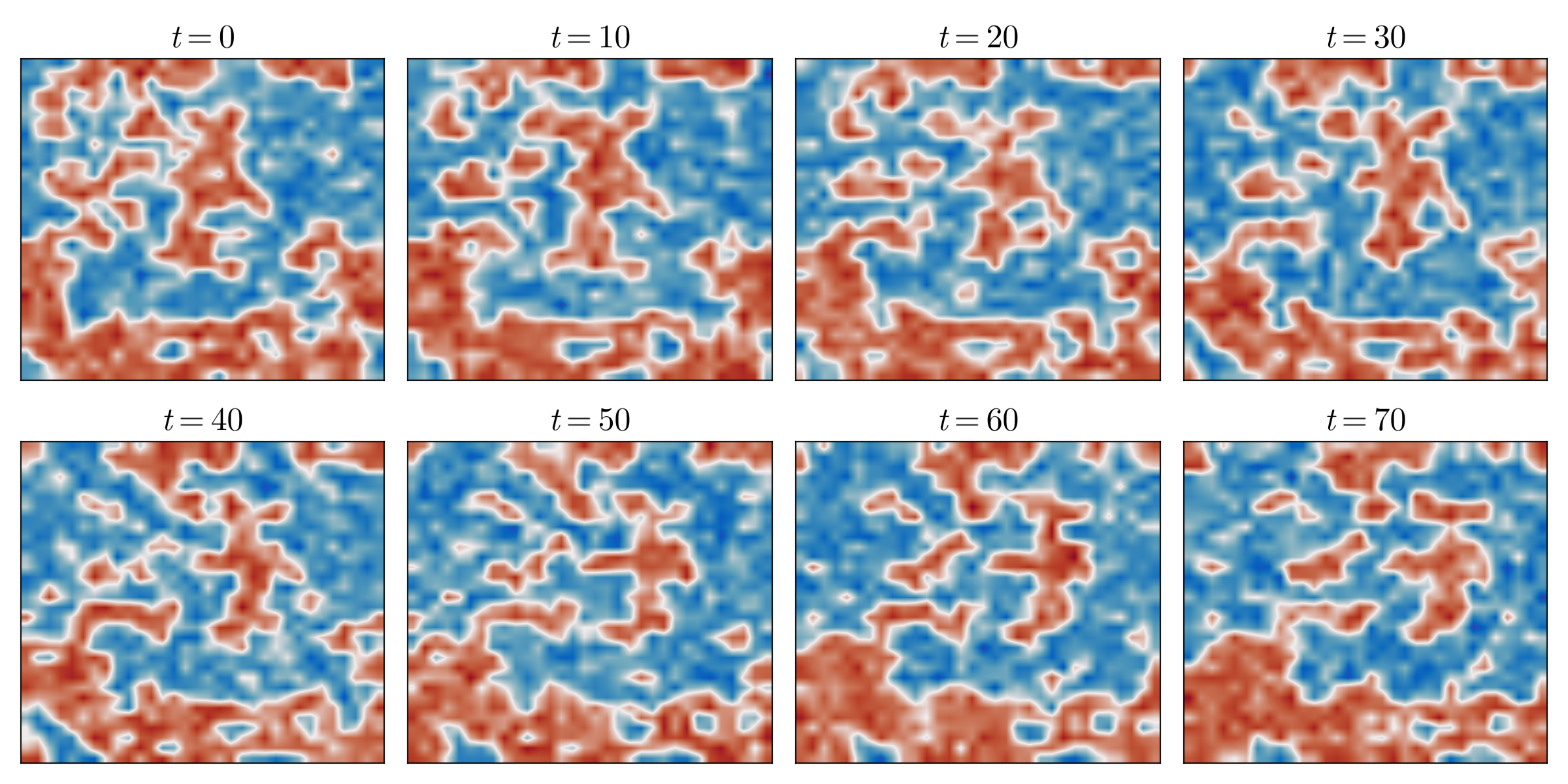
Figure 1: Example trajectory of the Allen-Cahn equation. Time progresses from $0$ to $70$ time units from top left to bottom right. We used approximately uncorrelated snapshots - sampled every 100 units of time - in training. Both the periodicity of the solution at the boundaries and the advection (to the right) are also visible in the trajectory.

The response function can also be estimated using numerical simulations of the dynamical system. This involves taking an ensemble of initial conditions, perturbing them, and evolving the unperturbed and perturbed system forward in time. The response can then be estimated using Equation (2) and Equation (2.1). However, this must be repeated for each perturbation of interest, and hence involves repeated simulation of the system, at a possibly large computational cost.

3 Denoising Score Matching

In this section, we focus on estimating the score function of the attractor of a dynamical system, as defined in Equation (4), through a denoising score matching training procedure often used in generative modeling (e.g., Song & Ermon, 2019; Song et al., 2020, and follow-on studies). This process approximates the score with a trainable function and subsequently optimizes its parameters. In principle, this could be achieved by minimizing an explicit score-matching loss function in which a trainable function is compared to the exact score. However, the true score function $\bm{s}(\bm{u})$ is generally unknown.

To overcome this problem, we perturb the data across a continuum of noise scales as is done in (Sohl-Dickstein et al., 2015; Song & Ermon, 2019; Ho et al., 2020) by using a forward diffusion process governed by the stochastic differential equation (SDE; Song et al. (2020)).

$$\,\mathrm{d}_{l}\bm{u}=\bm{\xi}_{l},$$ (6)

where $l$ is a diffusion time not to be confused with the physical time of the dynamical system from the previous section. Here, we employ a notation common in the physical sciences, rather than using the Wiener process differential $\,\mathrm{d}\bm{W}$. Note that we consider a discretized version of $\bm{u}$ on an $N\times N$ grid, such that the dimensionality of the discretized $\bm{u}$ is $N^{2}$. Furthermore, $\bm{\xi}_{l}$ is a $N^{2}$-dimensional zero-mean random normal vector with diagonal covariance matrix and variance $g_{l}^{2}$ for all components of $\bm{\xi}_{l}$. The initial condition for Equation (6) is drawn from the steady-state distribution (e.g., the attractor):

$$\bm{u}_{0}\sim\rho.$$ (7)

The solution of Equation (6) at any diffusion time $l$, $\bm{u}_{l}$, follows a multivariate Gaussian distribution

$$\bm{u}_{l}\sim\mathcal{N}(\bm{u}_{0},\sigma^{2}_{l}\mathbb{I}),$$ (8)

with diagonal covariance matrix $\sigma^{2}_{l}\mathbb{I}$ governed by the variance

$$\sigma^{2}_{l}=\int_{0}^{l}g_{l^{\prime}}^{2}\,\mathrm{d}l^{\prime}.$$ (9)

The function $g_{l}$ is chosen to grow exponentially with diffusion time $l$ so that at $l=1$ the variance is much larger than the original scale of the data points. As a result the final distribution of the $\bm{u}_{1}$ can be approximated as

$$\bm{u}_{1}\approx\mathcal{N}(\bm{0},\sigma^{2}_{1}\mathbb{I}).$$ (10)

This is referred to as the “variance-exploding” form of the forward diffusion process (Song et al., 2020). This choice ensures that the memory of the initial condition in the diffusion process is lost, mapping points in the observed space $\bm{u}_{0}$ to points in the latent space $\bm{u}_{1}$ drawn from a known distribution independent of the source data. Since the score function $\bm{s}(\bm{u},l)$ of the forward diffusion process changes smoothly with $l$, it is easier to learn using the denoising score matching loss (Song et al., 2020). We choose a suitable function approximator (e.g., a neural network) and train it with the denoising score matching loss given by

$$\mathcal{L}(\bm{\theta})=\mathbb{E}\left[\Big{\|}\sigma_{l}\bm{s}_{\bm{\theta}}(\bm{u}_{0}+\sigma_{l}\bm{\epsilon})+\bm{\epsilon}\Big{\|}^{2}\right],$$ (11)

where the expectation $\mathbb{E}$ is a shorthand for $\mathbb{E}_{l\sim\mathcal{U}_{[0,1]},\bm{u}_{0}\sim\rho,\bm{\epsilon}\sim\mathcal{N}(\bm{0},\mathbb{I})}$ (Song et al., 2020). Note that the actual loss function employed in training differs slightly from (11); it is described in Appendix C.

Having trained the score function $\bm{s}_{\bm{\theta}}(\bm{u},l)$ we can use it to estimate the score of the steady-state (e.g., the attractor) $\rho(\bm{u})$ to use it as a drop-in score estimator within the context of Equation (2.1). This is accomplished by simply setting $l=0$ as input to the trained score model so that we have

$$\bm{s}(\bm{u})\approx\bm{s}_{\bm{\theta}}(\bm{u},0).$$ (12)

Note that in many applications, the score function $\bm{s}_{\bm{\theta}}(\bm{u},l)$ is used to generate synthetic data samples using the reverse process of Equation (6) (Anderson, 1982). However, in this work, we use the reverse process only to assess the quality of the learned score function during training. We are otherwise not interested in generating samples.

4 Experiments

Reaction-diffusion equations (Kolmogorov et al., ) are partial differential equations combining a diffusive term with a (non)linear reaction term. They are commonly used to study pattern formation (e.g., Turing (1990); Callahan & Knobloch (1999); Kondo & Miura (2010)) and chemical processes. In this section we apply the method proposed in the previous sections to estimate the response function of a reaction-diffusion equation using score-based generative modeling. We compare the results to a numerical response computed by solving the perturbed dynamical system, a response using an analytically derived score function, and the response obtained through the Gaussian approximation frequently used in the literature. Both the numerically determined response function and that based on the analytic estimate of the score can be interpreted as “truth”, but note that in many cases neither of these baseline “truths” will be attainable due to analytic intractability, the large computational cost require to compute the response function numerically, or inability to attain the underlying system that generated the time-series.

For a detailed exposition of the construction methodology of the response matrix $R_{ij}(\tau)$ for all cases, please refer to Appendix B. With respect to the details of the training and validation of the score model, we refer the reader to Appendix C.

4.1 A Modified Allen-Cahn System

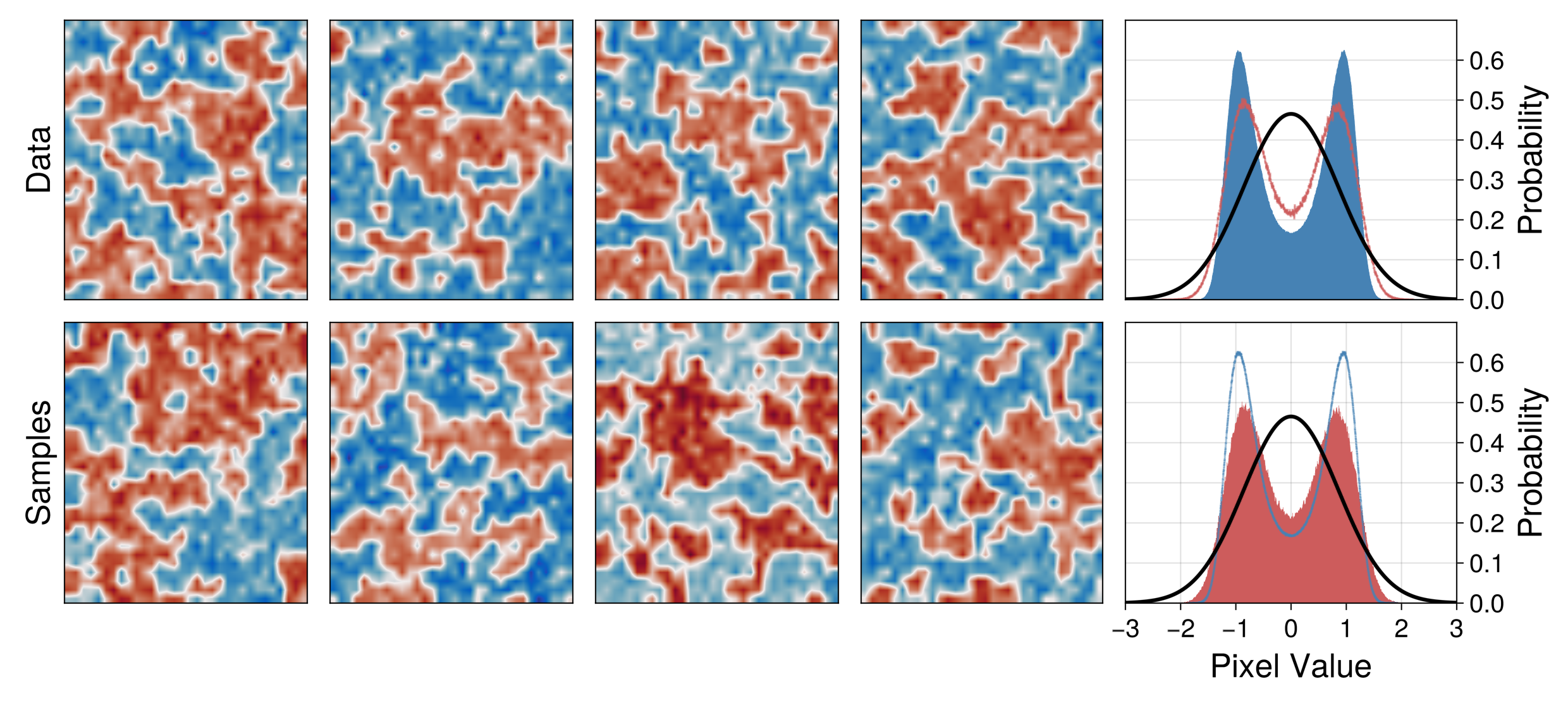
Figure 2: Example snapshots and steady-state pixel distribution of the solution to the Allen-Cahn equation. In the top row, we show the results of a numerical simulation of Equation (15) on a domain of size $2\pi\times 2\pi$ using $32\times 32$ pixels; in the bottom row, we show example samples generated by sampling with the learned score function using reverse diffusion (Song et al., 2020). The rightmost column shows the corresponding pixel distributions, where the blue and red lines indicate the equivalent distributions from the top and bottom, respectively. The black line shows the Gaussian approximation fitted to the bimodal pixel distribution.

The Allen-Cahn system is an example of a reaction-diffusion equation used for modeling phase separation in multi-component systems (see Allen & Cahn, 1972, who studied applications to binary alloys). It is defined by the following stochastic partial differential equation

$$\partial_{t}\bm{u}=\Delta\bm{u}+\bm{u}(1-\bm{u}^{2})+\epsilon\bm{\xi},$$ (13)

where $\bm{u}=\bm{u}(\bm{x},t)$ is the unknown field which depends on space $\bm{x}$ and time $t$. Furthermore, $\epsilon$ is a constant scalar setting the amplitude of the stochastic forcing and $\bm{\xi}$ represents space-time noise with covariance

$$\mathbb{C}\textrm{ov}\left[\bm{\xi}(\bm{x},t)\right]=\delta(\bm{x}-\bm{x}^{\prime},t-t^{\prime}),$$ (14)

where $\delta(\bm{x},t)$ is the Dirac delta function. Here, we adjust the system to include an advection term and spatially correlated noise, as follows,

$$\partial_{t}\bm{u}=\kappa\Delta\bm{u}-U\partial_{x}\bm{u}+\alpha\Sigma\left(\bm{u}(1-\bm{u}^{2})\right)+\epsilon\Sigma^{1/2}\bm{\xi},$$ (15)

where $\Sigma\equiv(1-\Delta)^{-1}$ is the inverse Helmholtz operator, and $U$, $\alpha$, $\kappa$ are constants. We take the spatial domain to be periodic. In this work, the field $\bm{u}$ maps a two-dimensional location into a scalar field, which we represent with a spatial discretization of $N^{2}$ degrees of freedom (or pixels, when representing the field as an image). In our study, we used $N=32$ pixels.

The advection term, $U\partial_{x}\bm{u}$, was added because it introduces a preferred direction of information propagation and therefore a direction of causality. This equation generates steady-state trajectories exhibiting non-Gaussian and bimodal statistics. The bimodal nature arises because the potential function of the system has two global minima, at $\bm{u}=\pm\bm{1}$. The correlated noise is necessary to allow for spatially local transitions between $\pm 1$. Despite this complexity, it retains an analytically tractable score function, as derived in Appendix A,

$$\bm{s}(\bm{u})=\frac{2}{\epsilon^{2}}\left[\alpha\bm{u}(1-\bm{u}^{2})+\kappa(\Delta\bm{u}-\Delta^{2}\bm{u})\right].$$ (16)

The analytic score function and the machine-learned score will differ by a constant factor due to the difference between the Kronecker delta and the Dirac delta functions. In our example, the analytic score function is $32^{2}$ larger. We divide the analytic score by this factor for comparison with the machine-learned score. The availability of the analytic score makes the system a good candidate for exploring the comparative performance between different estimates of the response function (analytic, numerically estimated with the dynamical system, Gaussian-approximated, and machine-learned).

To train the score model, we generated 25,000 uncorrelated snapshots by numerically timestepping the discretized system corresponding to Equation (15). For the spatial discretization, we use a spectral method Boyd (2001), and for the temporal discretization, we used a Runge-Kutta 4 scheme for the deterministic dynamics and accounted for the noise term after the final Runge-Kutta stage. An example trajectory is shown in Figure 1. The two modes, red and blue, correspond to two phases of the field.

Example training data samples and the steady-state pixel distribution of the numerically simulated system are shown in the upper row of Figure 2. As described in Section 3, the training process produces a calibrated function that approximates the score function as a function of diffusion time. This can be used to generate samples, and in the bottom row of Figure 2, we show examples of the generated field and the corresponding steady-state pixel distribution. Further validation of the score model using these samples was carried out and is discussed in Appendix C. For our purposes, however, we focus on using the score model evaluated at a diffusion time of zero, as in Equation (12), to generate the response function.

In comparing the steady-state pixel distributions of both the generated fields and data samples to the Gaussian distribution defined by the data’s mean and variance (as used in the Gaussian approximation), a notable limitation emerges. This approach does not capture the bimodal nature of the data distribution, a fact that is clearly visible in the rightmost panels of Figure (2). Although the match is not perfect, the bimodality is represented in the data generated using the score function. We found that increasing the training data from 6,000 samples to 25,000 greatly improved the pixel distribution of the generated samples. We anticipate that further augmenting the data would continue to improve the pixel distribution.

4.2 Response Function Results

Here we present the resulting score functions for the modified Allen-Cahn system generated using the four computation methods (exact analytic score, dynamical, Gaussian, and generative). We choose parameters $\alpha=8\times 10^{3/2}$, $\epsilon=2\times 10^{-3/2}$, $\kappa=2.5\times 10^{-4}$, $U=2\times 10^{-2}$, take the domain to be $2\pi$ periodic in each direction, and use timesteps of size $dt=1/32$. The methodology for calculating response functions is outlined in Appendix (B). We employed a timeseries of 2000 points (spaced in time by $t=1$ time units) and 128 ensemble members for the computation of response functions using both the Gaussian approximation and generative modeling techniques.

Owing to the periodic boundary conditions, the response matrix elements exhibit translational invariance: it depends only on the distance between pixels. This invariance implies that the index $i$ in the response matrix $R_{ij}$ can be arbitrarily fixed. We chose $j=1$ and calculated the response matrix elements along the direction of advection (denoted by $i$), as this is the direction information propagation, where we observe a larger response to perturbations at pixel component $i=1$.

The resulting responses of nearby pixels as a function of time are presented in Figure (3). For this system, the distance between adjacent pixels divided by the advection velocity $U$ gives a travel time of approximately $10$, which is clearly observed and captured by all response functions. However, the figure illustrates that the response matrix elements computed using the score function from generative modeling more accurately reproduce the true response (either numerically computed or analytically derived) than those obtained via the Gaussian approximation for the full nonlinear system.

To quantify the performance in the nonlinear case, we report root-mean-square-errors (RMSE) between the exact analytic estimate and the generative score model estimate, and between the analytic estimate and the Gaussian estimate, in Table 1.

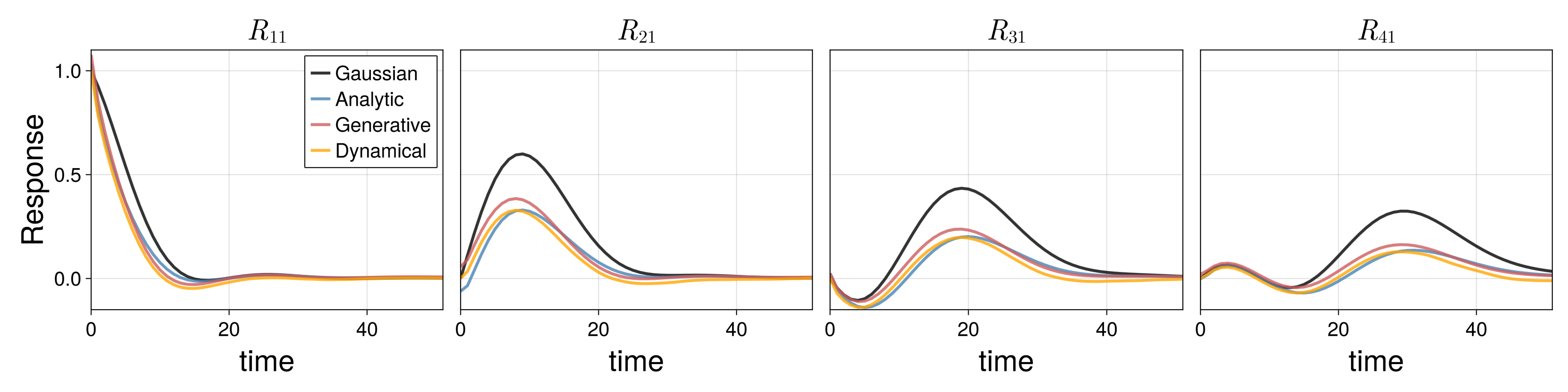
Figure 3: Response functions for the Allen-Cahn system. The response to a perturbation at the pixel component $i=1$, evaluated at various pixel components whose coordinates are indicated atop each panel. All evaluated components align with the advection direction. Responses are computed integrating the dynamical system (orange lines, “Dynamical”), via Gaussian approximation (black lines, “Gaussian”), using the score function derived from generative modeling (red lines, “Generative”), and using the analytic score function (blue lines, “Analytic”).

RMSE Table
Method	$R_{11}$	$R_{21}$	$R_{31}$	$R_{41}$
Score-model	0.12	0.32	0.23	0.18
Gaussian	0.46	0.95	0.90	0.76

Table 1: Root-mean-squared-errors (RMSE) of the response functions, obtained using the generative score-model and the Gaussian approximation, respectively, and computed using the analytic response function as baseline over the first 50 time units. See Figure 3. The columns denote the response of a pixel (0,1,2,3) units away from a perturbed pixel. The rows indicate the two methods.

5 Conclusions

In this study, we use score-based diffusion models to compute response functions. This offers a purely data-driven method to calculate accurate response functions. We have validated this approach on a version of the stochastic Allen-Cahn equation, an example of a reaction-diffusion equation, a class of SPDEs which have applications across biology, chemistry, and physics. We discretized the system spatially to $32\times 32$ interacting degree of freedom. We compared the response function of the system computed in four ways: using an analytic expression for the score, using the learned score function, using perturbations to initial conditions and solving the equations of motion, and using a Gaussian approximation. In this case, we found that the Gaussian response function over-predicted the response of pixels to neighboring perturbations, and that the score-based response function agreed well with both the numerically determined and analytic response functions. Compared with the Gaussian response, the RMSE of the score-model based response function reduced error by a factor of two to four.

This study addresses a gap in existing methodologies for analyzing high-dimensional dynamical systems, demonstrates additional utility of using score-based diffusion models, and sets the stage for future research. A natural next step would be to apply this method to more complex real-world systems found in the natural sciences.

The codes utilized in this research are publicly available for further study and replication in the following GitHub repository: https://anonymous.4open.science/r/PrivateGenLRT-052E/generate/allen_cahn_model.jl.

Broader Impact

This research uses recent advances in generative modeling to enhance the study of high-dimensional systems, with implications in fields such as climate science, financial markets and neuroscience. The improvement in our understanding of complex dynamics in these areas can lead to positive societal outcomes, such as more effective climate action through accurate forecasting, improved economic stability from enhanced financial risk assessment, and advancements in healthcare and well-being by deepening our understanding of neural processes.

Appendix A Derivation of Score for the Modified Allen-Cahn Equation

The potential function for the modified Allen-Cahn system (e.g., Equation (15)) is given by the following integral

$$\mathcal{V}[\bm{u}]=\frac{2}{\epsilon^{2}}\int\left[\frac{\alpha}{4}(1-\bm{u}^{2})^{2}+\frac{\kappa}{2}\left(|\nabla\bm{u}|^{2}+|\Delta\bm{u}|^{2}\right)\right]\,\mathrm{d}\bm{x},$$ (17)

where the parameters are defined in the main text. In steady-state, the probability density (or Gibbs measure) is given by Corwin & Shen (2020)

$$\rho(\bm{u})\propto\exp\left(-\mathcal{V}\right),$$ (18)

which yields the score function

$$\bm{s}(\bm{u})=-\frac{\delta\mathcal{V}}{\delta\bm{u}}=\frac{2}{\epsilon^{2}}\left[\alpha\bm{u}(1-\bm{u}^{2})+\kappa(\Delta-\Delta^{2})\bm{u}\right].$$ (19)

We comment that the fluctuation dissipation relation at time $t=0$ is

$$-\int\mathcal{D}[\bm{u}]\bm{u}\bm{s}(\bm{u})\rho(\bm{u})=\delta(\bm{x}-\bm{y}),$$ (20)

which differs from the discrete version by $\delta_{ij}$ to $\delta(\bm{x}-\bm{y})$. Here, we used a path integral notation for the previous equation. The presence of the correlated noise yields dynamics of the form

$$\partial_{t}\bm{u}=-\frac{\epsilon^{2}}{2}\Sigma\frac{\delta\mathcal{V}}{\delta\bm{u}}+\epsilon\Sigma^{1/2}\xi,$$ (21)

which is exactly Equation 15 without the advection term $U\partial_{x}\bm{u}$. To see that the advection term does not affect the steady-state distribution only requires changing reference frames to one with a velocity $U$ and making use of the translational invariance of the probability density. Alternatively, one can directly show from the Fokker-Planck equation that the advection term vanishes if one makes the ansatz that Equation 18 holds. The reason the advection term vanishes is two-fold, the first is that the trace of the advection operator is zero, the second observation is

$$\int(U\partial_{x}\bm{u})\frac{\delta\mathcal{V}}{\delta\bm{u}}\,\mathrm{d}\bm{x}=0,$$ (22)

in a periodic domain for a constant velocity $U$. For some more details on the topic see Corwin & Shen (2020).

Appendix B Construction of the Response Matrix

This section details the construction of the response matrix $R_{ij}(t)$, as referenced in Equation (2.1), which is used to estimate the response functions.

B.1 Derivation of the response function using the Gaussian approximation

In this section we derive the response function using the Gaussian approximation presented in Equation (5). The Gaussian approximation consists in approximating the unperturbed steady-state distribution $\rho$ with a multivariate Gaussian distribution

$$\rho_{G}(\bm{u})=\frac{1}{(2\pi)^{D/2}(\textrm{det}\,\bm{\Sigma})^{1/2}}\textrm{exp}\left(-\frac{1}{2}\bm{u}^{\textrm{T}}\bm{\Sigma}^{-1}\bm{u}\right),$$ (23)

with $\bm{\Sigma}$ the correlation matrix $\bm{C}(0)$ calculated for $t=0$. Using Equation (4), we can write the score function as

$$\bm{s}_{G}(\bm{u})=-\bm{\Sigma}^{-1}\bm{u}.$$ (24)

The response matrix then becomes

$$\bm{R}_{G}(\tau)=\langle\bm{u}(\tau)\bm{u}^{\textrm{T}}(0)\rangle_{\mathcal{J}}\bm{\Sigma}^{-1}=\bm{C}(t)\bm{C}^{-1}(0).$$ (25)

B.2 Dynamical Construction of the Response Matrix

Using Equation (2.1) and considering an infinitesimal delta function perturbation $\bm{\delta u}(0)=[0,\dots,\delta u_{j}(0),\dots,0]$, we arrive at the following expression for the response matrix:

$$R_{ij}(\tau)=\frac{\langle\delta u_{i}(\tau)\rangle_{p}}{\delta u_{j}(0)}.$$ (26)

Here, $\langle\delta u_{i}(\tau)\rangle_{p}$ is defined as in Equation (2). Initial conditions $\bm{u}(0)$ are drawn from the steady-state distribution, $\rho$. Each initial condition is perturbed to $\bm{v}(0)=\bm{u}(0)+\bm{\delta u}(0)$ for a fixed perturbation. The base trajectory and accompanying perturbed trajectory are integrated forward in time with the same sequence of noise. The difference between the two at each time $\tau$ yields $\delta u_{i}(\tau)$ and this term is then averaged over all initial conditions drawn from the steady-state distribution to yield $\langle\delta u_{i}(\tau)\rangle_{p}$. This methodology is replicated for all pixel values $j$, each time perturbing the system at a different pixel component.

Appendix C Score Model Training Details

C.1 Architecture

The network architecture used is based on a U-Net (Ronneberger et al., 2015). Three downsampling layers are used, followed by eight residual blocks, followed up by three upsampling layers. Convolutional kernels of size 3 x 3 pixels are used throughout. The diffusion time $l$ is embedded using a Gaussian Fourier projection (Tancik et al., 2020). Following Bischoff & Deck (2023), the image of spatial variations about the spatial mean is processed by the U-Net to produce the spatial variations about the spatial mean of the score, while the spatial mean of the image (a scalar) is processed using a simple feed forward network with two layers to produce the spatial mean of the score. We made use of the publicly available Julia code https://github.com/CliMA/CliMAgen.jl/ for the score-model training and sampling. We used the default settings for the model architecture. Please note that the convolutions used in the score model network respect the periodicity of the system using periodic padding.

C.2 Training

We split the data into a training dataset and a testing dataset using a 4:1 ratio. We use an Adam optimizer with $\epsilon=1e^{-8}$, $\beta_{1}=0.9$, and $\beta_{2}=0.999$ (Kingma & Ba, 2014). We normalize the gradient at each step, and use a warmup period of $5000$ gradient updates to linearly increase the learning rate to $2e^{-4}$ from $0$. The score-model was trained for 300 epochs. As the pixel values were already centered on zero with a variance near $1$, we did not further standardize the data. During training, we also kept track of a version of the model with exponential-moving-average (EMA) smoothed parameters. Using EMA parameters has been shown to improve model performance (Song et al., 2020). We used a memory parameter of $0.999$.

C.3 Loss Function

As noted in the main text, Equation (11) is not the exact form of the loss function used. The main differences are that the score network takes time as an independent argument and that it is parameterized as

$$\bm{s}_{\theta}(\bm{u},l)=\frac{\bm{f}_{\theta}(\bm{u},l)}{\sigma_{l}},$$ (27)

where $\bm{f}_{\theta}(\bm{u},l)$ is a trainable function and $\sigma_{l}$ is the conditional standard deviation of the forward diffusion process. This allows the function $\bm{f}_{\theta}(\bm{u},l)$ to target a quantity of order unity (e.g., Song & Ermon, 2019; 2020; Ho et al., 2020). Furthermore, following the same authors, we adjust the loss with the weighting function $\lambda(l)=\sigma_{l}$, so that the loss function decomposes into two part

$$\mathcal{L}(\theta)=\mathbb{E}_{l\sim\mathcal{U}[0,1],\bm{u}_{0}\sim\rho,\bm{u}_{l}\sim\mathcal{N}(\bm{u}_{0},\mathbb{I}\sigma^{2}_{l})}\left[\|\bar{\bm{f}}_{\bm{\theta}}(\bm{u}_{l},l)-\bar{\bm{\epsilon}}\|^{2}+\|\bm{f}_{\bm{\theta}}^{\prime}(\bm{u}_{l},l)-\bm{\epsilon}^{\prime}\|^{2}\right],$$ (28a)

where primes denote spatial variations about the mean, and overbars indicate spatial means. The Reynolds decomposition of the function $\bm{f}_{\theta}$ was first used in Bischoff & Deck (2023), and is the default option in the codebase https://github.com/CliMA/CliMAgen.jl/.

C.4 Noise Schedule

The prescribed variance schedule is presented in Song et al. (2020) and is called Variance Exploding (VE) schedule. We have for the noise scale and conditional variance of the noising process

$$g_{l} =\sigma_{\textrm{min}}\left(\frac{\sigma_{\textrm{max}}}{\sigma_{\textrm{min}}}\right)^{l}\sqrt{2\,\textrm{log}\left(\frac{\sigma_{\textrm{max}}}{\sigma_{\textrm{min}}}\right)}$$ (29a)

$$\sigma^{2}_{l} =\sigma_{\textrm{min}}^{2}\left[\left(\frac{\sigma_{\textrm{max}}}{\sigma_{\textrm{min}}}\right)^{2l}-1\right]\approx\sigma_{\textrm{min}}^{2}\left(\frac{\sigma_{\textrm{max}}}{\sigma_{\textrm{min}}}\right)^{2l},$$ (29b)

where $\sigma_{\textrm{min}}$ and $\sigma_{\textrm{max}}$ are scalar parameters determining the shape of the variance with time. Suitable values of these parameters can be computed from the data (Song & Ermon, 2020), e.g., $\sigma_{max}$ is given by the largest pairwise L2-distance in the dataset. For our dataset, we used $\sigma_{\rm{max}}=28$ and $\sigma_{\rm{min}}=1e^{-2}$.

C.5 Model Validation

To validate the learned score function, we numerically solved the reverse SDE using an Euler-Maruyama timestepper with initial condition $\bm{u}_{1}$ drawn from the approximate latent distribution at $l=1$, e.g., $\bm{u}_{1}\sim\mathcal{N}(\bm{0},\sigma_{\rm max}\mathbb{I})$ (Song et al., 2020). The diffusion time interval $l\in[1,0]$ was split into $250$ equally spaced steps.

We generated 2,000 samples using the reverse diffusion sampling strategy. Various statistical metrics (power spectra, the first four moments of the pixel value distribution) were computed using these synthetic samples and using samples from the real training data in order to assess the quality of the model. We ascertained that the power spectra and moments computed with both sample sets agreed within the uncertainties due to finite sample size, and we also visually inspected loss curves to assess whether training was converged.

References

- Arx (2020) High-dimensional inference: a statistical mechanics perspective. arXiv preprint arXiv:2010.14863, 2020.
- Arx (2021) Efficient state and parameter estimation for high-dimensional nonlinear system identification with application to meg brain network modeling. arXiv preprint arXiv:2104.02827, 2021.
- Adcock et al. (2020) Adcock, B., Brugiapaglia, S., Dexter, N., and Moraga, S. Deep neural networks are effective at learning high-dimensional hilbert-valued functions from limited data. arXiv preprint arXiv:2012.06081, 2020.
- Allen & Cahn (1972) Allen, S. M. and Cahn, J. W. Ground state structures in ordered binary alloys with second neighbor interactions. Acta Metallurgica, 20(3):423–433, 1972.
- Anderson (1982) Anderson, B. D. Reverse-time diffusion equation models. Stochastic Processes and their Applications, 12(3):313–326, 1982.
- Aurell & Del Ferraro (2016) Aurell, E. and Del Ferraro, G. Causal analysis, correlation-response, and dynamic cavity. In Journal of Physics: Conference Series, volume 699, pp. 012002. IOP Publishing, 2016.
- Authors (Yeara) Authors. Deep learning of causal structures in high dimensions under data limitations. Nature Machine Intelligence, Number(Number):Pages, Yeara.
- Authors (Yearb) Authors. Large-scale nonlinear granger causality for inferring directed dependence from short multivariate time-series data. Scientific Reports, Number(Number):Pages, Yearb.
- Badwan (2022) Badwan, N. Perspective Chapter: International Financial Markets and Financial Capital Flows - Forms, Factors and Assessment Tools. IntechOpen, 2022. doi: 10.5772/intechopen.102572. URL https://www.intechopen.com/chapters/80683.
- Baldovin et al. (2020) Baldovin, M., Cecconi, F., and Vulpiani, A. Understanding causation via correlations and linear response theory. Physical Review Research, 2(4):043436, 2020.
- Barabási & Albert (1999) Barabási, A.-L. and Albert, R. Emergence of scaling in random networks. Science, 286:509–512, 1999.
- Beneventano et al. (2021) Beneventano, P., Cheridito, P., Graeber, R., Jentzen, A., and Kuckuck, B. Deep neural network approximation theory for high-dimensional functions. arXiv preprint arXiv:2112.14523, 2021.
- Bischoff & Deck (2023) Bischoff, T. and Deck, K. Unpaired downscaling of fluid flows with diffusion bridges. arXiv preprint arXiv:2305.01822, 2023.
- Boyd (2001) Boyd, J. P. Chebyshev and Fourier Spectral Methods. Dover Books on Mathematics. Dover Publications, Mineola, NY, second edition, 2001. ISBN 0486411834 9780486411835.
- BozorgMagham et al. (2015) BozorgMagham, A. E., Motesharrei, S., Penny, S. G., and Kalnay, E. Causality analysis: Identifying the leading element in a coupled dynamical system. PLOS ONE, 10(6):e0131226, 2015.
- Branicki & Majda (2012) Branicki, M. and Majda, A. J. Quantifying uncertainty for predictions with model error in non-gaussian systems with intermittency. Nonlinearity, 25(9):2543, 2012.
- Brunton et al. (2019) Brunton, S. L., Noack, B. R., and Koumoutsakos, P. Machine learning for fluid mechanics. Annual Review of Fluid Mechanics, 52:477–508, 2019.
- Callahan & Knobloch (1999) Callahan, T. and Knobloch, E. Pattern formation in three-dimensional reaction–diffusion systems. Physica D: Nonlinear Phenomena, 132(3):339–362, 1999.
- Camps-Valls et al. (2023) Camps-Valls, G., Gerhardus, A., Ninad, U., Varando, G., Martius, G., Balaguer-Ballester, E., Vinuesa, R., Diaz, E., Zanna, L., and Runge, J. Discovering causal relations and equations from data. arXiv preprint arXiv:2305.13341, 2023.
- Corwin & Shen (2020) Corwin, I. and Shen, H. Some recent progress in singular stochastic partial differential equations. Bulletin of the American Mathematical Sociefty, 57(3):409–454, 2020.
- Daum (2005) Daum, F. Nonlinear filters: beyond the kalman filter. IEEE Aerospace and Electronic Systems Magazine, 20(8):57–69, 2005.
- Dorogovtsev et al. (2008) Dorogovtsev, S. N., Goltsev, A. V., and Mendes, J. F. F. Critical phenomena in complex networks. Reviews of Modern Physics, 80:1275, 2008.
- Falasca et al. (2023) Falasca, F., Perezhogin, P., and Zanna, L. A data-driven framework for dimensionality reduction and causal inference in climate fields. 2023. doi: 10.48550/arXiv.2306.14433. URL https://arxiv.org/abs/2306.14433.
- Friedrich et al. (2011) Friedrich, R., Peinke, J., Sahimi, M., and Tabar, M. R. R. Approaching complexity by stochastic methods: From biological systems to turbulence. Physics Reports, 506(5):87–162, 2011.
- Ghil & Lucarini (2020) Ghil, M. and Lucarini, V. The physics of climate variability and climate change. Reviews of Modern Physics, 92(3):035002, 2020.
- Granger (1969) Granger, C. W. Investigating causal relations by econometric models and cross-spectral methods. Econometrica: journal of the Econometric Society, pp. 424–438, 1969.
- Gritsun & Branstator (2007) Gritsun, A. and Branstator, G. Climate response using a three-dimensional operator based on the fluctuation–dissipation theorem. Journal of the atmospheric sciences, 64(7):2558–2575, 2007.
- Halu et al. (2013) Halu, A., Mondragón, R. J., Panzarasa, P., and Bianconi, G. Multiplex pagerank. PLoS ONE, 8:e78293, 2013.
- Ho et al. (2020) Ho, J., Jain, A., and Abbeel, P. Denoising diffusion probabilistic models. Advances in neural information processing systems, 33:6840–6851, 2020.
- Hunt et al. (2021) Hunt, B. A., Tewarie, P. K., Smith, A. G. G., Porcaro, C., Singh, K. D., and Murphy, P. R. Network modeling of dynamic brain interactions predicts emergence of neural information that supports human cognitive behavior. PLOS Biology, 2021. doi: 10.1371/journal.pbio.3001686. URL https://journals.plos.org/plosbiology/article?id=10.1371/journal.pbio.3001686.
- Jumper et al. (2021) Jumper, J. et al. Highly accurate protein structure prediction with alphafold. Nature, 596:583–589, 2021.
- Kaddour et al. (2022) Kaddour, J., Lynch, A., Liu, Q., Kusner, M. J., and Silva, R. Causal machine learning: A survey and open problems. arXiv preprint arXiv:2206.15475, 2022.
- Keyes et al. (2023) Keyes, N. D. B., Giorgini, L. T., and Wettlaufer, J. S. Stochastic paleoclimatology: Modeling the epica ice core climate records. Chaos: An Interdisciplinary Journal of Nonlinear Science, 33(9):093132, 2023.
- Kingma & Ba (2014) Kingma, D. P. and Ba, J. Adam: A method for stochastic optimization. arXiv preprint arXiv:1412.6980, 2014.
- (35) Kolmogorov, A., Petrovskii, I., and Piskunov, N. A study of the diffusion equation with increase in the amount of substance, and its application to a biological problem. übersetzung aus: Bulletin of the moscow state university series a 1: 1-26, 1937. Selected Works of AN Kolmogorov, 1.
- Kondo & Miura (2010) Kondo, S. and Miura, T. Reaction-diffusion model as a framework for understanding biological pattern formation. science, 329(5999):1616–1620, 2010.
- Kriegeskorte & Wei (2021) Kriegeskorte, N. and Wei, X.-X. Neural tuning and representational geometry. Nature Reviews Neuroscience, 22(11):703–718, 2021.
- Loikith & Neelin (2015) Loikith, P. C. and Neelin, J. D. Short-tailed temperature distributions over north america and implications for future changes in extremes. Geophysical Research Letters, 42(20):8577–8585, 2015.
- Lucarini (2018) Lucarini, V. Revising and extending the linear response theory for statistical mechanical systems: Evaluating observables as predictors and predictands. Journal of Statistical Physics, 173(6):1698–1721, 2018.
- Marconi et al. (2008) Marconi, U. M. B., Puglisi, A., Rondoni, L., and Vulpiani, A. Fluctuation–dissipation: response theory in statistical physics. Physics reports, 461(4-6):111–195, 2008.
- Martin et al. (2021) Martin, Z., Son, S.-W., Butler, A., Hendon, H., Kim, H., Sobel, A., Yoden, S., and Zhang, C. The influence of the quasi-biennial oscillation on the madden–julian oscillation. Nature Reviews Earth & Environment, 2(7):477–489, 2021.
- Mucha et al. (2010) Mucha, P. J., Richardson, T., Macon, K., Porter, M. A., and Onnela, J.-P. Community structure in time-dependent, multiscale, and multiplex networks. Science, 328:876–878, 2010.
- Pearl (2009) Pearl, J. Causal inference in statistics: An overview. 2009.
- Proistosescu et al. (2016) Proistosescu, C., Rhines, A., and Huybers, P. Identification and interpretation of nonnormality in atmospheric time series. Geophysical Research Letters, 43(10):5425–5434, 2016.
- Ronneberger et al. (2015) Ronneberger, O., Fischer, P., and Brox, T. U-net: Convolutional networks for biomedical image segmentation. In Medical Image Computing and Computer-Assisted Intervention–MICCAI 2015: 18th International Conference, Munich, Germany, October 5-9, 2015, Proceedings, Part III 18, pp. 234–241. Springer, 2015.
- Schreiber (2000) Schreiber, T. Measuring information transfer. Physical review letters, 85(2):461, 2000.
- Sjöberg et al. (2009) Sjöberg, P., Lötstedt, P., and Elf, J. Fokker–planck approximation of the master equation in molecular biology. Computing and Visualization in Science, 12:37–50, 2009.
- Sohl-Dickstein et al. (2015) Sohl-Dickstein, J., Weiss, E., Maheswaranathan, N., and Ganguli, S. Deep unsupervised learning using nonequilibrium thermodynamics. In International conference on machine learning, pp. 2256–2265. PMLR, 2015.
- Song & Ermon (2019) Song, Y. and Ermon, S. Generative modeling by estimating gradients of the data distribution. Advances in neural information processing systems, 32, 2019.
- Song & Ermon (2020) Song, Y. and Ermon, S. Improved techniques for training score-based generative models. Advances in neural information processing systems, 33:12438–12448, 2020.
- Song et al. (2020) Song, Y., Sohl-Dickstein, J., Kingma, D. P., Kumar, A., Ermon, S., and Poole, B. Score-based generative modeling through stochastic differential equations. arXiv preprint arXiv:2011.13456, 2020.
- Sporns & Betzel (2021) Sporns, O. and Betzel, R. F. Contributions and challenges for network models in cognitive neuroscience. Nature Neuroscience, 2021. doi: 10.1038/s41593-021-00858-0. URL https://www.nature.com/articles/s41593-021-00858-0.
- Stanczuk et al. (2023) Stanczuk, J., Batzolis, G., Deveney, T., and Schönlieb, C.-B. Your diffusion model secretly knows the dimension of the data manifold, 2023.
- Tancik et al. (2020) Tancik, M., Srinivasan, P., Mildenhall, B., Fridovich-Keil, S., Raghavan, N., Singhal, U., Ramamoorthi, R., Barron, J., and Ng, R. Fourier features let networks learn high frequency functions in low dimensional domains. Advances in Neural Information Processing Systems, 33:7537–7547, 2020.
- Timmermann et al. (2018) Timmermann, A., An, S.-I., Kug, J.-S., Jin, F.-F., Cai, W., Capotondi, A., Cobb, K. M., Lengaigne, M., McPhaden, M. J., Stuecker, M. F., et al. El niño–southern oscillation complexity. Nature, 559(7715):535–545, 2018.
- Turing (1990) Turing, A. M. The chemical basis of morphogenesis. Bulletin of mathematical biology, 52:153–197, 1990.
- Vincent (2011) Vincent, P. A connection between score matching and denoising autoencoders. Neural computation, 23(7):1661–1674, 2011.