Quantifying analogy of concepts via ologs and wiring diagrams

Abstract.

We build on the theory of ontology logs (ologs) created by Spivak and Kent, and define a notion of wiring diagrams. In this article, a wiring diagram is a finite directed labelled graph. The labels correspond to types in an olog; they can also be interpreted as readings of sensors in an autonomous system. As such, wiring diagrams can be used as a framework for an autonomous system to form abstract concepts. We show that the graphs underlying skeleton wiring diagrams form a category. This allows skeleton wiring diagrams to be compared and manipulated using techniques from both graph theory and category theory. We also extend the usual definition of graph edit distance to the case of wiring diagrams by using operations only available to wiring diagrams, leading to a metric on the set of all skeleton wiring diagrams. In the end, we give an extended example on calculating the distance between two concepts represented by wiring diagrams, and explain how to apply our framework to any application domain.

1. Introduction

Analogical reasoning is a technique that humans often use in problem-solving. We apply analogical reasoning when we are dealing with a problem in a new situation, where the problem bears some resemblance to ones that we have solved before. In a more mundane, everyday situation, this could mean figuring out how to catch a train in a city we have never been in - from past experiences, we might gather that a plan that has a good chance of working is to buy a ticket first, and then find the right platform for the train. Of course, the details as to how to purchase a ticket and how to find a specific train platform would vary from location to location, but as long as we attempt to execute steps that are ‘close’ to the plan we have in mind, or ‘similar’ to steps that we had taken in the past for getting onto the right train, our plan has a reasonable chance of succeeding. We also use analogical reasoning in situations that are much more nuanced and complex, such as in scientific research, in setting government policies, or in legal arguments in the courtroom. The recognition of analogues is also important in human experiences, such as in art, literature, and music.

In order to apply analogical reasoning in designing a problem-solving framework by autonomous systems, we first need a way to recognize when two concepts are similar. In other words, we need a way to quantify the similarity between two concepts. Although there are existing methods for quantifying analogy such as word-embedding algorithms [13, 4], these methods use statistical or probabilistic techniques that rely on having enough data, which is not always how humans recognize analogies. Humans can recognize analogies by determining the internal structures of concepts and by categorizing concepts [8].

In this article, we describe a mathematical approach to quantifying the analogy of two concepts. Our approach builds on the idea of ontology logs, or ologs, first coined in a paper by Spivak and Kent in 2012 [20]. Ologs gives a direct connection between data (such as those received from sensors in an autonomous machine) and category theory (a part of mathematics that studies the relations among objects, independent of context). In particular, we define the notion of wiring diagrams, which are labelled directed graphs satisfying certain axioms. Wiring diagrams can be used to represent processes that occur over time, and hence can be used to represent complex concepts. The labels of wiring diagrams correspond to concepts that appear as objects in ologs, whereas the underlying directed graphs of wiring diagrams themselves form a category. Since ologs are themselves categories, we can compare wiring diagrams using both the underlying graph structures and the underlying categorical structures, thus quantifying the similarity between two concepts (as long as they are represented as wiring diagrams).

1.1 O

logs give a way to organize concepts and the relations among them. Every olog is a category in the sense of category theory, which is a language that is used across major branches of modern mathematics. In addition, every olog is associated to a database schema. As a result, ologs provide a bridge via which tools from different areas of mathematics such as algebra, topology and geometry can be used to organize and understand data. Indeed, ologs have been applied to fields such as biology [19, 24], linguistics [12], materials design and manufacturing [6, 3], among others.

1.2

para:intro-WD Wiring diagrams have long been used to represent the various components and connections in an electric circuit. Mathematically, wiring diagrams can be defined and studied as operads [15, 17, 21, 25]. In this article, we settle for a more simplistic definition of a wiring diagram - roughly speaking, a directed graph with labels that correspond to objects in an olog. Of course, it would be interesting to work out the precise connections between the operadic approach towards studying discrete-time processes taken in [15] and our approach.

1.3 I

n Section 2, we give a brief example to illustrate the basic terminology from the theory of ologs. In Section 3, we review the idea that any classification scheme for concepts that involves a series of ‘multiple-choice’ questions - such as the dichotomous identification key for insects that students may learn in high school - can be constructed as an olog. We also list in Section LABEL:para:tipspopulateolog basic ideas for populating an olog for use in a specific application domain. In Section 4, we demonstrate how intangible concepts such as relations among physical entities can be represented by ologs. We also point out the obvious fact, that since an olog has an underlying graph, one can use any reasonable metric on graphs such as the shortest-distance metric to define a distance between any two objects in an olog.

In Section 5, we give the mathematical definition of our version of wiring diagrams. We prove a couple of elementary mathematical properties of wiring diagrams in Lemmas 5.5 and 5.5. Then, through an example in LABEL:eg:buyingcoffee, we illustrate how the occurence of a concept that is represented by a wiring diagram can be detected using data collected from sensors over time.

In Section 6, we define the notion of skeleton wiring diagram graphs, or skeleton WD graphs. These are directed graphs that are the underlying graphs of skeleton wiring diagrams. We show in Section LABEL:para:catskWDgs that skeleton WD graphs with a common set $V$ of vertices form a category $\mathcal{R}(V)$. As such, morphisms in this category give us new ways to compare wiring diagrams, i.e. new ways to compare concepts, that were not possible if one only considered traditional edit operations on graphs. Then in Section LABEL:sec:distanceedit-WD, we use morphisms in the category $\mathcal{R}(V)$ to extend the usual definition of elementary edit operations on graphs to the case of wiring diagrams.

In Section 7, we give an extended example showing how the ideas in Sections 5 and 6 can be implemented to quantify the analogy between two concepts. We chose the concepts of an ‘electric car charging station’ and a ‘bus’. Both are physical entities that are capable of changing a characteristic of another physical entity when a particular relation is satisfied. We explain how to define relevant sensors and ologs, and then how to construct wiring diagrams that can be used to represent the two concepts ‘electric car charging station’ and ‘bus’. Then, we show how elementary edit operations on wiring diagrams can be used to define a ‘distance’ between these two concepts, thus achieving our goal of quantifying analogy between concepts that are represented by wiring diagrams. In LABEL:para:summaryofcalc, we give a list of steps that one can follow in order to implement the ideas in this article to quantify analogy in any application domain of the reader’s choice. Finally, we end the article with a brief discussion on future directions in Section 8.

1.4 T

he author would like to thank David I Spivak and Nima Jafari for helpful comments on earlier versions of the manuscript. This work was partially supported by a DARPA Young Faculty Award (number D21AP10109-02).

2. Ologs and data

We assume the reader has a rudimentary knowledge of the language of category theory and ologs, including the concept of fiber product (or ‘pullback’) in a category. Basic concepts in category theory can be found in books such as [18, 22, 1] which are aimed at a general audience, or [9] which is aimed at mathematicians. On the other hand, a quick introduction to ologs can be found in the paper by Spivak and Kent [20, Sections 1-3] in which ologs were first defined. In this section, we briefly recall some basic terminology from the theory of ologs by way of an example. We will also assume throughout this article that all the categories that arise are small.

2.1 A

n olog is a category in which

• Each object and each arrow is labeled with text to indicate their meaning.

• Each arrow represents a relation that corresponds to a function.

Property (ii) is one of the main differences between the olog approach and the knowledge graph approach to knowledge representation. It implies that any two consecutive arrows can be composed (because any two functions where the codomain of one equals the domain of the other can be composed), which is one of the requirements of a category. Since an olog is a category, which has an underlying graph, both graph-theoretic and category-theoretic tools are available when dealing with ologs.

For example, Figure 1 is an olog with three objects and two arrows. In this olog, given any pair $(p,c)$ where $p$ is a person, $c$ is a car, and $p$ owns $c$, the arrow $p$ (resp. $c$) represents the operation that “forgets” the information $c$ (resp. $p$) and only remembers $p$ (resp. $c$); using a more mathematical language, we can think of $p$ and $c$ as the first and second projections from the ordered pair $(p,c)$, respectively.

Figure 1. An example of an olog.

We will follow the language in [20], and refer to objects in an olog as types, arrows in an olog as aspects, and write $\lceil$something$\rceil$ instead of when we want to refer to a type in the main text of this article. We will also use the notation $\dashv$p$\vdash$ when we refer to an aspect labelled as $p$.

We can regard an olog as a representation of the internal knowledge of an autonomous system. In this article, we will focus on ologs where, for every point $t$ in time, each type ${\mathcal{T}}$ in an olog corresponds to a table ${\mathcal{F}}_{t}({\mathcal{T}})$ containing all instances of the concept ${\mathcal{T}}$ known to the autonomous system. For example, suppose at the point $t$ in time, there are 5 persons known to the system, say Adam, Betty, Carlos, Dolly, Eric, and 4 cars known to the system, say (labeled by their license plate numbers) 9XL3A, 2HA1T, 8WT9R, 5RV3Q, 6PK7M. Suppose also that at time $t$, the system is aware that Betty owns the car 9XL3A, Carlos owns 6PK7M, and that Dolly owns 5RV3Q. Then the three types in Figure 1 would yield the three tables in Table 1, which together constitute a simple database containing data that corresponds to the concepts in the olog in Figure 1. The rows of these tables are called the instances of the corresponding type. The arrows $p$ and $c$ in Figure 1 then yield the operations ${\mathcal{F}}_{t}(p),{\mathcal{F}}_{t}(c)$ which, respectively, sends each pair in the middle table to either the first coordinate (‘person’) or the second coordinate (‘car’). For example, ${\mathcal{F}}_{t}(p)$ would send the pair ‘(Betty, 9XL3A)’ to ‘Betty’ while ${\mathcal{F}}_{t}(c)$ would send it to ‘9XL3A’. In the language of category theory, we say that ${\mathcal{F}}_{t}$ is a functor. (See [20, 18] for more on the connections between ologs and database schemas.)

Person
Adam
Betty
Carlos
Dolly
Eric

(a) Table for the type $\lceil$a person$\rceil$

Pair $(p,c)$ where
person $p$ owns car $c$
(Betty, 9XL3A)
(Carlos, 6PK7M)
(Dolly, 5RV3Q)

(b) Table for the type $\lceil$a pair $(p,c)$ where person $p$ owns car $c$$\rceil$

Car
9XL3A
2HA1T
8WT9R
5RV3Q
6PK7M

(c) Table for the type $\lceil$a car$\rceil$

Table 1. Tables that together form a database.

3. Using ologs to classify concepts

Since an olog is defined to be a category in the mathematical sense, all the tools in category theory apply to ologs. The fiber product construction in category theory, for example, offers a way to make precise the ‘overlap’ or intersection of two concepts. Using fiber products, any scheme that classifies a collection of concepts via a series of multiple-choice questions, such as a flow chart for identifying insects that are often taught in high school biology can be incorporated into an olog.

3.1

para:classifytoolog Consider the following series of questions, which might be used as part of a scheme that tries to classify different types of transport vehicles:

• Question 1: Does it have wheels? Answer:

  • Yes

  • No

• Question 2: What power source does it use? Answer:

  • Human power.

  • Electricity.

  • Gas.

Recording the answers to these questions when we apply them to a bicycle and a gas-powered car, we obtain the table in Table 2.

Question	Bicycle	Gas-powered car
Question 1	1	1
Question 2	1	3

Table 2.

The answers recorded in Table 2 allow us to associate the concepts ‘bicycle’ and ‘gas-powered car’ to different vectors in $\mathbb{R}^{2}$

bicycle $$\mapsto(1,1)$$

gas-powered car $$\mapsto(1,3).$$

The point here, however, is that we can construct an olog that distinguishes $\lceil$a bicycle$\rceil$ and $\lceil$a gas-powered car$\rceil$ as two distinct types. To do this, let us begin with the simple olog in (3.1.1), which represents the fact ‘a bicycle is a human-powered vehicle’.

(3.1.1)

The database schema corresponding to this olog consists of two tables: a table listing all known instances of a bicycle, and a table listing all known instances of a human-powered vehicle, such that every instance that appears in the first table also appears in the second table. Table 3 shows an example of such a schema.

Bicycle
Bicycle 1
Bicycle 2
Bicycle 3

(a) Table for the type $\lceil$a bicycle$\rceil$

Human-powered

vehicle

Kayak 1

Bicycle 1

Kayak 2

Bicycle 2

Skateboard 1

Bicycle 3

(b) Table for the type $\lceil$a human-powered vehicle$\rceil$

Table 3. An example of tables in a database schema for the olog in Figure 3.1.1.

Intuitively, the concept of a human-powered vehicle represents the overlap of two different concepts: a transport vehicle, and the use of human power. More concretely, a human-powered vehicle can be defined as a transport vehicle that uses human power as a source of power. As a result, in the setting of ologs, we can construct the type $\lceil$a human-powered vehicle$\rceil$ using a fiber product as follows. We begin with the olog in (3.1.2), where the vertical arrow is the function that takes any transport vehicle as its input, and gives its type of power source (e.g. human power, gas, electricity, etc.) as its output.

(3.1.2)

The pullback of the olog in (3.1.2) is (3.1.3), in which the upper and the left arrows are newly generated in the pullback construction. The upper row represents the fact ‘a human-powered vehicle is a transport vehicle’, and the left vertical arrow represents the same function as the right vertical arrow (in this case, every instance of a human-powered vehicle uses human power as its power source, and so the codomain of the left vertical arrow is simply ‘human power’).

(3.1.3)

Similarly, we can construct the concept $\lceil$a gas-powered vehicle$\rceil$ in an olog using a fiber product as in (3.1.4).

(3.1.4)

Since the right vertical arrows in (3.1.3) and (3.1.4) coincide, both of these ologs can be incorporated into the larger olog in (3.1.5).

(3.1.5)

The olog (3.1.5) ‘recovers’ Question 2 in the multiple-choice classification scheme from the start of this subsection. To find the answer when we apply Question 2 to the concept ‘a bicycle’, for example, we look among types $B$ that correspond to the upper-left vertex of a fiber product diagram of the form in (3.1.6), where $A$ is a type corresponding to a specific example of a power source, and find the particular $B$ such that there is an injection $\dashv$is$\vdash$ pointing from $\lceil$a bicycle$\rceil$ to $B$.

(3.1.6)

3.2

para:tipspopulateolog The examples in Section LABEL:para:classifytoolog cover some basic principles for populating an olog for applications in a given context:

1. Introduce types that correspond to ‘seed’ concepts that are relevant to the given context. For example, in the case of the olog in (3.1.5), we can begin with $\lceil$a transport vehicle$\rceil$, $\lceil$a type of power source$\rceil$, $\lceil$gas$\rceil$, and so on.

2. Introduce aspects that connect different seed concepts. In (3.1.5), this means introducing the function $\dashv$has as power source$\vdash$ and the two $\dashv$is$\vdash$ arrows from $\lceil$gas$\rceil$ and $\lceil$human power$\rceil$.

3. Perform categorical operations such as fiber products to generate more complicated types in the olog; these operations also come with natural arrows such as projections. In the case of (3.1.5), this entails constructing the two fiber products within it. These fiber products generate the new types $\lceil$a human-powered vehicle$\rceil$ and $\lceil$a gas-powered vehicle$\rceil$; we can then connect them with the types $\lceil$a bicycle$\rceil$ and $\lceil$a gas-powered passenger car$\rceil$ with respective $\dashv$is$\vdash$ arrows.

4. Distance between concepts in an olog

Once we have an olog that includes the relevant concepts in a particular context or application, we can start using the olog to define distances between pairs of concepts, thereby quantifying the similarity or ‘degree of analogy’ of different concepts. The idea is simple: every category has an underlying graph, and there are established methods for defining a notion of distance between vertices in a graph (e.g. see [23] and [7, D41]).

Definition 4.1. (shortest-distance metric on an olog)  Given an olog $O$, we can first consider the underlying graph, which is a directed graph. Suppose we forget the directions of the arrows and consider the associated undirected graph $G$. Let $V$ be the set of vertices of $G$, and $A$ the set of edges in $G$. Recall that a path from one vertex $x$ to another vertex $y$ is a sequence of edges $e_{1},\cdots,e_{m}$, for some positive integer $m$, that begins at $x$ and ends at $y$. Let us assume $G$ is a connected graph with a finite number vertices and edges. Then for any function $c:A\to\mathbb{R}_{>0}$, we can define a new function $d:V\times V\to\mathbb{R}_{\geq 0}$ via the formula

$$d(x,y)=\min\Bigl{\{}\sum_{i=1}^{n}c(e_{i}):\text{ there is a path $e_{1},\cdots,e_{n}$ from $x$ to $y$ in $G$}\Bigr{\}}.$$

It is easy to see that the function $d$ satisfies the requirements of a metric on the set $V$, thus giving us a notion of ‘distance’ between vertices of the graph $G$, and hence a notion of distance between types (concepts) in the olog $O$. If the olog $O$ has an underlying graph that is disconnected, we can simply enlarge the codomain of $d$ to $\mathbb{R}_{\geq 0}\cup\{\infty\}$ and define $d(x,y)$ to be $\infty$ when $x,y$ lie in distinct disconnected components of the graph.

Example 4.2. Consider the olog (3.1.5). If we assume the function $c$ in Definition 4 assigns the value $1$ to every edge in the underlying undirected graph of this olog, then with respect to the shortest-distance metric, the distance between the concepts ‘a bicycle’ and ‘a gas-powered passenger car’ would be 4, whereas the distance between the concepts ‘a human-powered vehicle’ and ‘a gas-powered vehicle’ would be 2.

Under the shortest-distance metric, the distance between two concepts depends on the function $c$, and hence the specific olog in use. If the olog (3.1.5) contains more types and aspects between $\lceil$a bicycle$\rceil$ and $\lceil$a human-powered vehicle$\rceil$, for instance, and $c$ still assigns the value $1$ to every edge, then the distance between the concepts ‘a bicycle’ and ‘a gas-powered passenger car’ would be greater than 3. This is not unreasonable since, even for a person, whether or not two concepts are similar depends on the particular context, and also on the amount of knowledge the person has.

4.3

sec:comparingrels Concepts that seem more intangible at first glance - such as relations among different entities - may also be represented as types in an olog. Once two concepts are represented by types in the same olog, we can use ideas from Section 4 to define a notion of distance between two relations.

The olog in Figure 1 already contains an example: we can represent the relation of ownership between a car and a person as the type $\lceil$a pair $(p,c)$ where person $p$ owns car $c\rceil$.

Between two entities, such a person $p$ and a car $c$, there may be different relations that one can speak of. For example, if a person $p$ owns a car $c$, then the two entities are related by an ‘ownership’ relation. If a different person $p^{\prime}$ owns a different car $c^{\prime}$, then $p^{\prime}$ and $c^{\prime}$ are related by the same relation. On the other hand, if the person $p$ has access to the car $c^{\prime}$ (e.g. $p$ leases the car $c$ but does not own it), then we can say $p$ and $c^{\prime}$ are related by an ‘access’ relation, which is different from the ‘ownership’ relation. In analogical reasoning, it is important to be able to compare different relations between the same entities.

We describe here a systematic way to construct types in an olog that represent relations between entities. Suppose $\thicksim$ is a relation between two entities, and we write $x\thicksim y$ to represent ‘$x$ is related to $y$ via the relation $\thicksim$’. Then we can always construct the types and aspects as in (4.3.1).

(4.3.1)

Here, $p_{1}$ and $p_{2}$ refers to projections from a pair $(x,y)$ to its first argument $x$ and second argument $y$, respectively. We can then use the type $P_{\thicksim}$ as a representation for the relation $\thicksim$ between an entity of kind $K_{1}$ and an entity of kind $K_{2}$.

Using fiber products, we can now construct types that represent various kinds of relations in an olog and understand how they are related to one another.

Example 4.4. Consider the olog in (4.4.1). To construct this olog, we first begin with the types $A,B$, and $A^{\prime}$. We then construct $D$ as the direct product of $B$ with itself, and define $p_{1},p_{2}$ as the projections onto the first and the second arguments, respectively. For convenience, given any two types $P,Q$ in this olog, we will write $PQ$ to denote the unique aspect in the olog from $P$ to $Q$. Then we construct $C^{\prime\prime}$ as the fiber product of $C^{\prime}D$ and $CD$.

Now, if we add the type $F$ to the olog as a proxy for the relation ‘ownership’ between two entities, we can further construct $E$ as the fiber product of $FD$ and $CD$, $E^{\prime}$ as the fiber product of $FD$ and $C^{\prime}D$, and $E^{\prime\prime}$ as the fiber product of $EF$ and $E^{\prime}F$. If we add another type $\widetilde{F}$ as a proxy for the relation ‘has access to’ between two entities, we can similarly construct $\widetilde{E}$ as the fiber product of $\widetilde{F}D$ and $CD$, $\widetilde{E}^{\prime}$ as the fiber product of $\widetilde{F}D$ and $C^{\prime}D$, and $\widetilde{E}^{\prime\prime}$ as the fiber product of $\widetilde{E}\widetilde{F}$ and $\widetilde{E}^{\prime}\widetilde{F}$.

Now, for the underlying undirected graph of the olog in (4.4.1), if we use a function $c$ that assigns the value $1$ to every edge, then with respect to the shortest-distance metric (Definition 4), the distance between the concepts ‘owns’ and ‘has access to’ would then be equal to 2 (attained by the path $FD$ followed by $D\widetilde{F}$. The distance between the concept ‘a person owning a building’ (represented by $E^{\prime\prime}$) and the concept ‘a person having access to a building’ (represented by $\widetilde{E}^{\prime\prime}$) would also be 2, attained by the path $E^{\prime\prime}C^{\prime\prime}$ followed by $C^{\prime\prime}\widetilde{E}^{\prime\prime}$.

One can imagine that, by using other types representing relations other than $F$ and $\widetilde{F}$, new types representing other relations among different kinds of entities can be added to the olog. As a result, we will be able to define a distance between any two relations as long as they appear as types in the same olog.

(4.4.1)

5. Using wiring diagrams to represent processes

In Section 3, we saw that fiber product from category theory can be used to build complex concepts from simple concepts. In this section, we introduce the idea of wiring diagrams, which will allow us to represent processes that occur over time. We will define a wiring diagram as a graph decorated with labels. Note that the idea of wiring diagrams has been used in engineering for many years, and there have been various mathematical approaches to using wiring diagrams to represent systems or processes [15, 17, 21]. In this article, we focus on a more elementary approach and leave a more operadic approach as taken in the aforementioned articles to future work.

Definition 5.1. A (directed) graph is a quadruple $G=(V,A,s,t)$ where

• $V$ is a set, the elements of which are called vertices;

• $A$ is a set, the elements of which are called arrows, or edges;

• $s:A\to V$ is a function, called the source function;

• $t:A\to V$ is a function, called the target function.

Given an arrow $a$ in a graph, we often draw it as an arrow pointing from $s(a)$ to $t(a)$:

$$s(a)\overset{a}{\longrightarrow}t(a).$$

That is, the functions $s$ and $t$ indicate where an arrow starts and end, respectively.

For example, Figure 2 is a graph with 4 vertices (labelled $A,B,C,D$) and 5 arrows (labelled $a,b,c,d,e$), with the functions $s,t$ given by $s(a)=A=s(b),t(a)=t(b)=s(c)=s(e)=B,t(c)=s(d)=C$, and $t(d)=t(e)=D$.

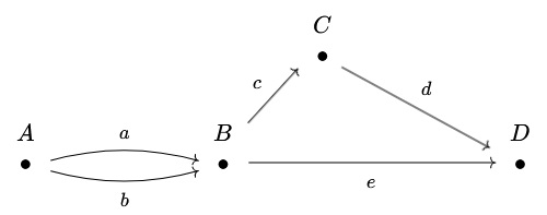
Figure 2.

A wiring diagram in this article will be a graph where, to each vertex, we attach a ‘state vector’ that represents the values of certain parameters that correspond to sensors. To make this precise, we first define the notion of sensing functions.

Definition 5.2. (sensing function)  A sensing function $F$ associated to a sensor is a function whose domain $D_{F}$ is the set of all the things the sensor can be applied to, and whose codomain $C_{F}$ is the set of all possible outputs from the sensor. That is, for any $x\in D$, $F(x)$ is the output given by the sensor.

We also allow sensors to take on broader meanings, and use the word sensor to refer to any device or algorithm that observes the environment and gives an output.

Example 5.3. (a) For a speed sensor next to a motorway, the corresponding sensing function $F$ can be defined on the set $D_{F}$ of all cars that move past the sensor, while $C_{F}$ is the set of all nonnegative integers. Then, at any point in time, $F$ would give an integer output representing the speed of a vehicle currently in front of the sensor (in miles per hour, rounded to the nearest nonnegative integer); if there is no vehicle in front of the sensor, the sensor gives an output of $0$.

(b) For a motion sensor that detects whether there is any movement inside a particular room, we can take the domain $D_{F}$ of the corresponding sensing function $F$ to be the singleton set $\{\bullet\}$, and take the codomain $C_{F}$ of $F$ to be $\{0,1\}$. This way, at any point in time, the sensing function $F$ would give the value $0$ if no movement is detected inside the room, and give the value $1$ if movement is detected.

(c) For a sensor that tracks the blood oxygen level of a particular person, the corresponding sensing function $F$ can be defined as a function from a singleton set $\{\bullet\}$ to the real interval $[0,100]$ so that, at any point in time, the number $F(\bullet)$ represents the blood oxygen level of that person (in percentage) at that time.

(d) For any two cities $x,y$ in the world, we can define a sensing function $F_{x,y}:\{\bullet\}\to\{0,1\}$, which depends on $x$ and $y$, such that $F_{x,y}(\bullet)$ takes on the value $1$ (resp. $0$) if $x$ and $y$ are sister cities (resp. are not sister cities). The value of $F_{x,y}$ would depend on the particular time when the measurement is taken. In practice, this sensing function can be constructed using an algorithm that crawls through the public web or government databases to determine the current status of sister city agreements between the two cities.

We now define a wiring diagram as follows.

Definition 5.4. (wiring diagram)  A wiring diagram (WD) is a quintuple

$$(V,A,s,t,\mathscr{L}_{V})$$

satisfying the following conditions.

1. $G=(V,A,s,t)$ is a finite directed graph, called the underlying graph of the wiring diagram. We will refer to elements of $V$ as vertices or states, and refer to elements of $A$ as arrows or wires.

2. $\mathscr{L}_{V}$ is an indexed set $\{L_{v}\}_{v\in V}$ such that each $L_{v}$ is a set of triples

   $$L_{v}=\{(F_{i},x_{i},y_{i}):1\leq i\leq m_{v}\}$$

   where $m_{v}$ is a nonnegative integer depending on $v$, and where each $F_{i}$ is a sensing function, with $x_{i}$ in the domain of $F_{i}$ and $y_{i}$ in the codomain of $F_{i}$. We allow $L_{v}$ to be the empty set.

3. There is a labelling of the vertices, given by a function $f:V\to\{1,2,\cdots,n\}$ where $n$ is the number of elements in $V$, such that for each $a\in A$, we have $f(s(a))<f(t(a))$.

In our formal definition above, we do not a priori require $f$ to be a bijective function. By Lemma 5.5 below, however, there always exists a bijection $f$ that satisfies WD2. By abuse of notation, we will refer to $L_{v}$ as the state vector at the vertex $v$, and refer to an element of $L_{v}$ as a label. We will refer to a graph that arises as the underlying graph of a wiring diagram as a wiring diagram graph or a WD graph. Note that a finite directed graph is a WD graph if and only if it satisfies WD2.

How to read a wiring diagram.

• For each vertex $v$, the state vector $L_{v}$ specifies the values of various parameters that must be achieved at a particular point in time.

• Each arrow $a$ represents the requirement that the state vector $L_{s(a)}$ is achieved before the state vector $L_{t(a)}$ is achieved.

Condition WD2 implies that we can always arrange the vertices of a wiring diagram in a way so that every arrow points from left to right. A wiring diagram then represents a process where, as we read the diagram from left to right, specific readings of parameter values occur.

5.5 W

e list some basic properties of WD graphs in this subsection.

We adopt the following definitions for a directed graph $G=(V,A,s,t)$.

• A loop is an arrow that points from a vertex to itself, i.e. $a\in A$ such that $t(a)=s(a)$.

• A path of length $n$ is a sequence of arrows $a_{1},\cdots,a_{n}$, where $n$ is a positive integer, such that $t(a_{i})=s(a_{i+1})$ for all $1\leq i\leq n-1$, and none of the $a_{i}$ are loops.

• An oriented cycle is a path of length more than 1 that begins and ends at the same vertex.

Note that an arrow is a path of length 1.

Lemma 5.6.  Let $G=(V,A,s,t)$ be a WD graph. Then

• $G$ contains no loops.

• $G$ contains no oriented cycles.

Proof.

Let $f$ be a function associated to $G$ in WD2.

(i) Given any arrow $a\in A$, we have $f(s(a))<f(t(a))$ which implies $s(a)$ and $t(a)$ must be distinct vertices, and so $a$ cannot be a loop.

(ii) Suppose $G$ contains an oriented cycle, i.e. a path formed by the concatenation of arrows $a_{1},a_{2},\cdots,a_{k},a_{k+1}$ where $t(a_{i})=s(a_{i+1})$ for $1\leq i\leq k$ while $t(a_{k+1})=s(a_{1})$. Then we have

$$f(s(a_{1}))<f(t(a_{1}))=f(s(a_{2}))<\cdots<f(t(a_{k}))=f(s(a_{k+1}))<f(t(a_{k+1}))=f(s(a_{1}))$$

whic is a contradiction.   ◼

Definition 5.7. We say a WD graph is axal if the function $f$ in WD2 can be taken to be a bijection.

That is, a finite directed graph with $n$ vertices is an axal WD graph if and only if the vertices can be labelled as $v_{1},\cdots,v_{n}$ such that every arrow points from $v_{i}$ to $v_{j}$ for some $1\leq i<j\leq n$ (so all the vertices lie on an axis, and all the arrows point in the positive direction of the axis). The lemma below shows that every WD graph is axal.

Lemma 5.8.  Let $G=(V,A,s,t)$ be a WD graph. Then there exists a bijective function $\widetilde{f}:V\to\{1,2,\cdots,n\}$ where $n=|V|$ such that for every arrow $a\in A$, we have $\widetilde{f}(s(a))<\widetilde{f}(t(a))$. That is, $G$ is axal.

Proof.

Let $f:V\to\{1,\cdots,n\}$ be a function associated to $G$ as in WD2. Without loss of generality, we can assume ${\mathrm{im}\,}f=\{1,\cdots,k\}$ for some integer $1\leq k\leq n$. For each $i\in{\mathrm{im}\,}f$, let $M_{i}$ denote the preimage of $i$, i.e. $M_{i}=f^{-1}(i)$, and let $m_{i}=|M_{i}|$, the number of vertices mapping onto $i$ under $f$. Let $m=\max\{m_{i}:i\in{\mathrm{im}\,}f\}$.

Now for each $i\in{\mathrm{im}\,}f$, let $\widetilde{f}_{i}$ denote any bijection

$$M_{i}\to\left\{i+\frac{1}{2m}j:0\leq j\leq m_{i}-1\right\}=:R_{i}.$$

We can then concatenate the $\widetilde{f}_{i}$ into a single function $\widetilde{f}^{\prime}$ on $V$, i.e. we set

$$\widetilde{f}^{\prime}:V \to\bigcup_{i\in{\mathrm{im}\,}f}R_{i}$$

$$v \mapsto\widetilde{f}_{i}(v)\text{\quad if $v\in M_{i}$}.$$

Note that $\widetilde{f}^{\prime}$ is a bijection, and so we can post-compose $\widetilde{f}^{\prime}$ with a unique order-preserving bijection onto $\{1,\cdots,n\}$ to form a function $\widetilde{f}$. We claim that $\widetilde{f}$ satisfies WD2.

Take any arrow $a\in A$. From the definition of $f$, we have $f(s(a))<f(t(a))$. By construction of $\widetilde{f}^{\prime}$, it follows that

$$\lfloor\widetilde{f}^{\prime}(s(a))\rfloor=f(s(a))<f(t(a))=\lfloor\widetilde{f}^{\prime}(t(a))\rfloor$$

(where $\lfloor-\rfloor$ denotes the floor function on real numbers). From the construction of $\widetilde{f}^{\prime}$, this means that $\widetilde{f}^{\prime}(s(a))$ and $\widetilde{f}^{\prime}(t(a))$ lie in distinct $R_{i}$ and $\widetilde{f}^{\prime}(s(a))<\widetilde{f}^{\prime}(t(a))$, which in turn implies $\widetilde{f}(s(a))<\widetilde{f}(t(a))$. That is, $\widetilde{f}$ satisfies WD2.   ◼

Remark 5.9. Using the language of order theory, given a function $f$ in condition WD2 in the definition of a wiring diagram, we obtain a partial order on the set $V$ of vertices if we declare $x\leq y$ whenever $f(x)<f(y)$. It is well-known that every partial order has a linear extension, and Lemma 5.5 constructs an explicit linear extension for a given $f$. The definition of a wiring diagram does not come with a fixed function $f$, however; condition WD2 merely asserts the existence of such a function.

5.10

sec:statesvsactions Informally, each state vector $L_{v}$ in a wiring diagram represents the ‘status’ of relevant parameters, whereas each wire $a$ in a wiring diagram represents a ‘difference of states’, and thus corresponds to an action or event that leads the state vector at $L_{s(a)}$ to become the state vector $L_{t(a)}$. If we define sensing functions carefully, a single state vector can also indicate the occurence of an action or an event.

Example 5.11.  For example, suppose we want to represent the concept “person $p$ enters coffee shop $s$” using a wiring diagram. Consider a sensor tracking the movement of the person $p$, where the sensor gives the output $0$ when $p$ is outside the coffee shop, and gives the output $1$ when $p$ is inside the coffee shop. This results in a sensing function $F_{1}$ with the singleton set $\{\bullet\}$ as the domain and defined by

$$F_{1}(\bullet)=\begin{cases}0&\text{ if $p$ is outside $s$}\\ 1&\text{ if $p$ is inside $s$}\end{cases}$$

at any point in time. The concept “person $p$ enters coffee shop $s$” can then be represented by the wiring diagram with two vertices as in (5.11.1).

(5.11.1)

In particular, the single wire in this wiring diagram informally represents the act of $p$ ‘entering’ the coffee shop $s$.

Another way to represent the concept “person $p$ enters coffee shop $s$” is by considering a ‘numerical derivative’ of $F_{1}$. Let us define a new sensing function $dF_{1}:\{\bullet\}\to\{-1,0,1\}$ given by

$$dF_{1}(\bullet)=(\text{current value of }F_{1})-(\text{value of }F_{1}\text{ five seconds ago}).$$

Then the occurrence of $p$ entering the coffee shop $s$ would correspond to the moment when the function $dF_{1}$ registers a value of $1$, and so the act of $p$ entering the coffee shop $s$ can also be represented by the following wiring diagram with a single vertex and no wires

Example 5.12.  In (5.12.1) there are three possible underlying graphs for wiring diagrams with four vertices. In a wiring diagram with underlying graph $G_{1}$, the state vectors must be achieved in the order of $L_{A},L_{B},L_{C}$, and then $L_{D}$. A situation where such a wiring diagram arises, for example, would be in curriculum planning. In the curriculum of a gentle introduction to calculus, for example, we can define the state vectors $L_{A}$ through $L_{D}$ to represent the following:

• $L_{A}$: A student has learned the definition of continuity.

• $L_{B}$: A student has learned to take limits of functions.

• $L_{C}$: A student has learned the definition of derivative.

• $L_{D}$: A student has learned to take the derivative of a polynomial function.

To formally write these as labels of a wiring diagram in terms of sensing functions, one can use sensing functions that register the scores on tests covering the respective topics.

(5.12.1)

In a wiring diagram with underlying graph $G_{2}$, the state vector $L_{A}$ must be achieved first; then $L_{B}$ and $L_{C}$ must be achieved, but between them it does not matter whether it is $L_{B}$ or $L_{C}$ that is achieved first. After both $L_{B},L_{C}$ have been achieved, $L_{D}$ must then be achieved. Our example in Section LABEL:eg:buyingcoffee involves a wiring diagram that contains $G_{2}$ as part of its underlying graph.

In the case of $G_{3}$, either $L_{A}$ or $L_{C}$ must be achieved first, although they can occur independently. The state vector $L_{D}$ can only be achieved after $L_{A},L_{C}$ have both been achieved, while $L_{B}$ can only be achieved after $L_{A}$ has been achieved. (Between $L_{B}$ and $L_{D}$, there is no requirement as to which should come first.) A situation where such a wiring diagram arises is when different teams work on a project continuously in relay. Suppose for any positive integer $i$, there is a team $T_{i}$, and that all these teams work on the same project in a factory. Then a wiring diagram with underlying graph $G_{3}$ would depict the process of ‘passing the baton’ from one team to the next if we take the state vectors to represent the following for any $i\geq 2$:

• $L_{A}$: $T_{i-1}$ has created instructions for $T_{i}$.

• $L_{B}$: $T_{i-1}$ has departed the factory.

• $L_{C}$: $T_{i}$ has arrived at the factory.

• $L_{D}$: $T_{i}$ has completed the instructions from $T_{i-1}$ and made new progress on the project.

A wiring diagram with underlying graph such as (5.12.2) would then represent the entire relay process.

(5.12.2)

5.13

eg:buyingcoffee Let us build on Example 5.10 and consider the process of “a person $p$ buying coffee from a shop $s$”. We can think of this process as comprising four components:

• $p$ enters the coffee shop $s$.

• $p$ makes payment for coffee.

• $p$ receives coffee.

• $p$ leaves the coffee shop $s$.

Depending on the type of shop, (ii) might occur before (iii), or (iii) might occur before (ii); it is reasonable to assume, however, that in most cases, (i) must occur before both (ii) and (iii), which must occur before (iv).

Next, we describe each of events (i) through (iv) in terms of sensors. We can use changes in the value of the sensing function $F_{1}$ from above to describe (i) and (iv). To describe the event (ii), consider a sensing function $F_{2}$ that detects whether a payment has been made by $p$ for coffee (this is something that can be detected as a change in the activity log in the cashier’s machine, or in the activity log of person $p$’s payment devices). That is, we can take $F_{2}$ to be a function with domain $\{\bullet\}$ such that

$$F_{2}(\bullet)=\begin{cases}0&\text{ if $p$ has not made a new payment for coffee}\\ 1&\text{ if $p$ has made a new payment for coffee}\end{cases}.$$

To describe the event (iii), we can define a sensing function $F_{3}$ that detects whether $p$ is holding coffee (such as from an image recognition algorithm), i.e.  $F_{3}$ has domain $\{\bullet\}$ and is given by

$$F_{3}(\bullet)=\begin{cases}0&\text{ if $p$ is not holding any coffee}\\ 1&\text{ if $p$ is holding coffee}\end{cases}.$$

The process of “a person $p$ buying coffee from a coffee shop $s$” can now be represented by the wiring diagram in (5.13.1).

(5.13.1)

Let us define numerical derivatives of $F_{2}$ and $F_{3}$ by setting

$$dF_{i}(\bullet)=(\text{current value of }F_{i})-(\text{value of }F_{i}\text{ five seconds ago}).$$

for $i=1,2,3$. Then the process of “a person $p$ buying coffee from a coffee shop $s$” can also be represented by the wiring diagram

(5.13.2)

In this wiring diagram, each of the four labels corresponds to an action by $p$.

5.14

sec:WDandologs Recall that every label in a wiring diagram is of the form $(F,x,y)$ where $F$ is a sensing function with some domain $D_{F}$ and codomain $C_{F}$. Fix an element $y_{0}$ of $C_{F}$. We can construct the olog (5.14.1), where each vertical square is constructed using a fiber product. The instances of the type $\lceil$an element $x$ of $D_{F}$, $F(x)=y_{0}\rceil$ correspond to labels of the form $(F,x,y_{0})$, and so we can take this type in the olog as a representation of the concept captured by the label $(F,x,y)$. This way, every label in a wiring diagram can be represented by a type in an olog. Since we can define the distance between any two types in an olog (Section 4), we can define the distance between any two labels in a wiring diagram once we represent them as types in the same olog.

(5.14.1)

5.15

sec:relnsfs Even though a label in a wiring diagram must be of the form $(F,x,y)$ by definition, this definition is broad enough to describe relations among entities. To see this, let us recall some basic terminology on relations on sets.

Given two sets $S$ and $T$, a binary relation $R$ on $S\times T$ is simply defined to be a subset of $S\times T$. For any $a\in S$ and $b\in T$, we say $a$ is related to $b$ or write $a\thicksim b$ (when $R$ is understood) to mean $(a,b)\in R$.

Given a set $S$, a binary relation $R$ on $S$ is defined to be a relation on $S\times S$. For a relation $R$ on a set $S$, we say $R$ is

• reflexive if $x\thicksim x$ for all $x\in S$;

• anti-symmetric if, whenever $x\thicksim y$ and $y\thicksim x$ for $x,y\in S$, it follows that $x=y$;

• transitive if, whenever $x\thicksim y$ and $y\thicksim z$ for $x,y,z\in S$, we have $x\thicksim z$.

A binary relation that is both reflexive and transitive is called a preorder; a preorder that is also anti-symmetric is called a partial order.

Given a relation $R$ on a set $A\times B$, we can define the function

$$q_{R}:A\times B\to\{0,1\}:(a,b)\mapsto\begin{cases}0&\text{ if $a\nsim b$}\\ 1&\text{if $a\thicksim b$}\end{cases}.$$

That is, $F$ is a function that detects whether a pair $(a,b)$ satisfies the relation $R$. If we write $i_{j}$ to denote the inclusion of $\{j\}$ into $\{0,1\}$ for $j=0,1$, then we can construct the olog (5.15.1) where each vertical square is a fiber product. Pairs $(a,b)$ that lie in $R$ are now instances of the type $P_{1}$, and so we can take $P_{1}$ as a type that represents the relation $R$.

(5.15.1)

Note that we can regard $q_{R}$ as a sensing function with domain $A\times B$ and codomain $\{0,1\}$; this way, the olog (5.15.1) is merely a special case of the olog (5.14.1). The concept “$a$ is related to $b$ with respect to the relation $R$” can now be represented by the label $(q_{R},(a,b),1)$ in a wiring diagram. Equivalently, we can rewrite the label as $(F,\bullet,1)$ where $F$ is the sensing function

$$F_{(a,b),R}:\{\bullet\}\to\{0,1\}:\bullet\mapsto\begin{cases}0&\text{ if $a\nsim b$}\\ 1&\text{ if $a\thicksim b$}\end{cases}.$$

Remark 5.16. In the previous section, we saw that every label in a wiring diagram can be represented by a type in an olog. In the current section, we saw that labels can represent whether two entities satisfy a relation.

6. Using wiring diagrams to quantify analogy

In Section 4, we saw that there is a way to define the distance between any two concepts that occur as types in the same olog. In Section LABEL:sec:comparingrels, we saw that the relations between different entities (such as ownership or access) can be represented as types in an olog. Then, in Section 5, we saw that wiring diagrams can represent processes that occur over a period of time, and that the labels at the vertices of a wiring diagram can be defined using concepts that occur in an olog. This allowed us to conclude in Section LABEL:sec:WDandologs that we can define the distance between any two labels in a wiring diagram, as long as they both correspond to types in the same olog.

In this section, we propose a definition of distance between any two wiring diagrams. Our definition builds on the idea of elementary edit operations between graphs - which leads to the notion of graph edit distance - taking advantage of the fact that every wiring diagram has an underlying graph. Our approach has two advantages compared to simply considering the graph edit distance between the underlying graphs, however. First, we consider categories generated by these graphs, which allow us to make better use of the inherent structures of wiring diagrams; second, since labels of wiring diagrams correspond to types in an olog, we also have a measure of distance among the labels themselves that takes into account the structure of the olog being used. That is, our definition refines graph edit distance by utilizing the categorical aspects of wiring diagrams.

6.1

para:catskWDgs All the wiring diagrams that have appeared in this article are ‘skeleton’ in the following sense:

Definition 6.2. We say a WD graph $G=(V,A,s,t)$ is skeleton if it satisfies the following condition:

• For any two distinct vertices $v,v^{\prime}\in V$, there is at most one path from $v$ to $v^{\prime}$.

We say a wiring diagram is skeleton if its underlying graph is skeleton.

In particular, for any two distinct vertices $v,v^{\prime}$ in a skeleton WD graph, the following are true:

• If there is already a path from $v$ to $v^{\prime}$ comprising more than one arrow, then there cannot be any arrow (a path of length $1$) from $v$ to $v^{\prime}$.

• There is at most one arrow from $v$ to $v^{\prime}$.

We now describe a construction that takes any skeleton WD graph and produces a partial order on its set of vertices. Suppose $G=(V,A,s,t)$ is a skeleton WD graph. First, we define a relation $R_{0}$ on $V$ by setting

$$R_{0}=\{(x,y)\in V\times V:x=s(a),y=t(a)\text{ for some }a\in A\}.$$

Next, we define the transitive closure $R_{2}$ of $R_{0}$ [7, D26, Chap. 3]. That is, we first define

$$R_{1}=R_{0}\bigcup\{(x,y)\in V\times V:x=y\},$$

and then declare an element $(x,y)$ of $V\times V$ to be in $R_{2}$ if and only if there is a sequence of elements $(x_{0},x_{1}),(x_{1},x_{2}),\cdots,(x_{k-1},x_{k})$ in $R_{1}$ with $k\geq 1$ such that $x_{0}=x$ and $x_{k}=y$. In other words, $R_{2}$ is the result of forcing reflexivity and transitivity on $R_{0}$. By construction, $R_{2}$ is a preorder on $V$ and $R_{0}\subseteq R_{2}$. We write $R(G)$ to denote $R_{2}$. Note that $R(G)$ depends only on $G$, and not a choice of the bijection $\widetilde{f}$ from Lemma 5.5.

Lemma 6.3.  Let $G$ be a skeleton WD graph, and $\widetilde{f}:V\to\{1,\cdots,n\}$ (where $n=|V|$) any bijection as in Lemma 5.5. Then

• For any element $(x,y)$ of $R(G)$ where $x\neq y$, we have $\widetilde{f}(x)<\widetilde{f}(y)$.

• If we identify $V$ with the set $\{1,\cdots,|V|\}$ via the bijection $\widetilde{f}$, then $R(G)$ is a subset of the natural preorder on $\mathbb{Z}$.

Proof.

(i) Take any $(x,y)\in R(G)$ such that $x\neq y$. From the construction above, there exists a sequence $(x_{0},x_{1}),(x_{1},x_{2}),\cdots,(x_{k-1},x_{k})$ in $R_{1}$ with $k\geq 1$ such that $x_{0}=x,x_{k}=y$. For each $0\leq i\leq k-1$, either $x_{i}=x_{i+1}$ in which case $\widetilde{f}(x_{i})=\widetilde{f}(x_{i+1})$, or $x_{i}\neq x_{i+1}$ in which case $(x_{i},x_{i+1})\in R_{0}$ and $\widetilde{f}(x_{i})<\widetilde{f}(x_{i+1})$. The claim then follows.

(ii) This follows immediately from (i).   ◼

From the construction of $R(G)$, it is clear that $R(G)$ is always a partial order on $V$. Lemma 6.1(ii) says that there is always an embedding of partial orders from $R(G)$ into the natural partial order $(\mathbb{Z},\leq)$.

For any finite set $V$, we can now define a category $\mathcal{R}(V)$. We will take the objects of $\mathcal{R}(V)$ to be skeleton WD graphs $G$ whose underlying set of vertices is exactly $V$. Given any two skeleton WD graphs $G_{1},G_{2}$, we will define a morphism $G_{1}\to G_{2}$ whenever $R(G_{2})\subseteq R(G_{1})$. (Note that $R(G_{1}),R(G_{2})$ are both subsets of $V\times V$.) More precisely, if we consider the category $\mathcal{P}(V\times V)$ of subsets of $V\times V$ where morphisms are set inclusions, then we declare a morphism $\alpha_{i}:G_{1}\to G_{2}$ in $\mathcal{R}(V)$ whenever there is a morphism $i:R(G_{2})\to R(G_{1})$ in $\mathcal{P}(V\times V)$. In particular, for any object $G$ in $\mathcal{R}(V)$, we declare the identity morphism on $G$ to be that corresponding to the identity function on $R(G)$. Given any two composable morphisms, say $\alpha_{i}:G_{1}\to G_{2}$ and $\alpha_{j}:G_{2}\to G_{3}$, we define the composition $\alpha_{j}\alpha_{i}$ to be $\alpha_{ij}$, i.e. the morphism corresponding to the composite set inclusion $ij:R(G_{3})\subseteq R(G_{1})$. It is easy to see that $\mathcal{R}(V)$ satisfies the axioms of a category. We will refer to $\mathcal{R}(V)$ as the category of skeleton WD graphs over $V$.

Sometimes, we will use $\Rightarrow$ to indicate a morphism in $\mathcal{R}(V)$ to better distinguish between the arrows within wiring diagrams themselves. We say a morphism $\alpha:G_{1}\to G_{2}$ in $\mathcal{R}(V)$ is irreducible if it cannot be written as the composition of two non-identity morphisms, i.e. if there is no skeleton WD graph $G_{3}$ such that $R(G_{2})\subsetneq R(G_{3})\subsetneq R(G_{1})$.

Example 6.4. Let $V$ be the set $\{A,B,C\}$. Then $\alpha,\alpha^{\prime}$ below are morphisms in the category $\mathcal{R}(V)$

(6.4.1)

The morphism $\alpha$ corresponds to the inclusion

$$\{(A,C),(B,C)\}\subseteq\{(A,B),(B,C),(A,C)\}$$

of subsets of $V\times V$ while the morphism $\alpha^{\prime}$ corresponds to the inclusion

$$\{(A,B),(A,C)\}\subseteq\{(A,B),(B,C),(A,C)\}.$$

Informally, having a morphism $G\to G^{\prime}$ in a category $\mathcal{R}(V)$ means that the partial order generated by $G^{\prime}$ is ‘more general’ (i.e. is a smaller subset of $V\times V$, and hence has ‘less restrictions’) than that generated by $G$.

6.5 M

orphisms in the category of skeleton WD graphs give us a way to compare intrinsic structures of wiring diagrams.

Let us return to the example in Section LABEL:eg:buyingcoffee, where we defined sensing functions $dF_{1},dF_{2},dF_{3}$ and used them to write down a wiring diagram as in (5.13.2) to represent the process of “person $p$ buying coffee from coffee shop $s$”. Different people might have come up with different wiring diagrams to represent the same process. Both wiring diagrams in (6.5.1) can represent the process of $p$ buying coffee from $s$, the difference being whether we require the person to pay for coffee before or after they receive it.

(6.5.1)

In practice, we would want to consider the two wiring diagrams in (6.5.1) as very ‘similar’ to the wiring diagram in (5.13.2); in fact, we would normally think of the two diagrams in (6.5.1) as special cases of that in (5.13.2). To make these comparisons mathematically precise, we can use the category of skeleton WD graphs.

For simplicity, let us write $A,B,C,D$ to denote the labels

$$(dF_{1},\bullet,1),\,\,\,(dF_{2},\bullet,1),\,\,\,(dF_{3},\bullet,1),\,\,\,(dF_{1},\bullet,-1),$$

respectively. Let $V$ be the set $\{A,B,C,D\}$, and consider the category $\mathcal{R}(V)$ of skeleton WD graphs over $V$. Then we have two morphisms $\alpha,\alpha^{\prime}$ in $\mathcal{R}(V)$ as in (6.5.2).

(6.5.2)

The morphisms $\alpha,\alpha^{\prime}$ can be considered as mathematical formulations of the similarities between these wiring diagrams.

Remark 6.6.  Even though there is a notion of a category of graphs, the morphisms $\alpha,\alpha^{\prime}$ cannot have been defined as morphisms of graphs. In fact, using a standard definition of a morphism between graphs [9, Section II.7], in (6.5.2) any morphism in the category of graphs from the upper left graph to the lower graph should take the arrow from $B$ to $C$ to some arrow from $B$ to $C$, whereas we do not have any arrow between $B$ and $C$ in the lower graph.

6.7

sec:distanceedit-G For undirected graphs, a standard method for measuring the similarity between graphs is to use the graph edit distance. To define graph edit distance, one first needs to decide on a set of elementary edit operations on graphs such as inserting or deleting a vertex, inserting or deleting an edge, or changing the label of a vertex or an edge. The graph edit distance between two graphs $G,G^{\prime}$ is then the minimum number of elementary operations needed in order to transform $G$ to $G^{\prime}$ (e.g. see [11, Section 3.1] or [14, 16, 5]). The graph edit distance is a metric on the set of all finite graphs.

6.8

sec:distanceedit-WD Since wiring diagrams can be considered as directed graphs where the vertices are labelled with state vectors, we can also define a version of the graph edit distance tailored to wiring diagrams. In fact, we will introduce new operations on graphs that are only possible by considering the intrinsic structures of wiring diagrams.

Let us write $W_{s}^{\bullet}$ to denote the set of all skeleton wiring diagrams where the state vector $L_{v}$ at every vertex $v$ is nonempty, and where the underlying graph has at least one vertex. To begin with, we define elementary edit operations on such wiring diagrams to be the following.

• Adding a new vertex with a nonempty state vector.

• Deleting a vertex along with its state vector.

• Adding a new label at a vertex.

• Deleting an existing label at a vertex.

• Changing an existing label at a vertex to a different label.

• Adding an arrow.

• Deleting an arrow.

• Replacing the underlying graph $G=(V,A,s,t)$ of a skeleton wiring diagram with another skeleton WD graph $G^{\prime}=(V^{\prime},A^{\prime},s^{\prime},t^{\prime})$, such that $V^{\prime}=V$ and there is an irreducible morphism $G\to G^{\prime}$ in $\mathcal{R}(V)$.

• Replacing the underlying graph $G=(V,A,s,t)$ of a skeleton wiring diagram with a another skeleton WD graph $G^{\ast}=(V^{\ast},A^{\ast},s^{\ast},t^{\ast})$, such that $V^{\ast}=V$ and there is an irreducible morphism $G^{\ast}\to G$ in $\mathcal{R}(V)$.

We require an elementary operation to take a wiring diagram in $W_{s}^{\bullet}$ to another wiring diagram in $W_{s}^{\bullet}$. For example, we cannot apply operation (iv) to a vertex if it results in the vertex having an empty state vector, while operation (vi) is only valid if condition WD2 continues to hold. We will write $\mathrm{EEO}(W_{s}^{\bullet})$ to represent the set of all possible elementary edit operations on $W_{s}^{\bullet}$.

Note that operations (viii) and (ix) only change the arrows in the underlying graph and do not change the state vectors at the vertices. As we saw in Remark 6.5, operations (viii) and (ix) cannot always be replaced with elementary edit operations of other types. Also, operations of types (i), (iii), (vi), (viii) are the inverses of operations of types (ii), (iv), (vii), (ix), respectively, while the inverse of an operation of type (v) is again of type (v).

If there is a sequence $E_{1},\cdots,E_{m}$ of elementary edit operations (where $m$ is a positive integer) that transforms a wiring diagram $W$ in $W_{s}^{\bullet}$ to another wiring diagram $W^{\prime}$ in $W_{s}^{\bullet}$, then we say $(E_{1},\cdots,E_{m})$ is an edit path from $W$ to $W^{\prime}$. Given two wiring diagrams $W,W^{\prime}$ in $W_{s}^{\bullet}$, we will write $P(W,W^{\prime})$ to denote the set of all edit paths $(E_{1},\cdots,E_{m})$ that transform $W$ to $W^{\prime}$. Note that the length $m$ of the edit path may be different for different paths.

Lemma 6.9.  Let $c$ be any function from $\mathrm{EEO}(W_{s}^{\bullet})$ to $\mathbb{R}_{>0}$. For any $W,W^{\prime}\in W_{s}^{\bullet}$, set

$$d(W,W^{\prime})=\min{\Bigl{\{}\sum_{i=1}^{m}c(E_{i}):(E_{1},\cdots,E_{m})\in P(W,W^{\prime})\Bigr{\}}}.$$

Then $d$ is a function $W_{s}^{\bullet}\times W_{s}^{\bullet}\to\mathbb{R}_{>0}$ that defines a metric on $W_{s}^{\bullet}$.

Proof.

Given any wiring diagram $W$ in $W_{s}^{\bullet}$, there is always a sequence of elementary edit operations of types (vii), (ii) and (iv) that transform $W$ into a wiring diagram with a single vertex and a single label. This means that for any two elements $W,W^{\prime}$ in $W_{s}^{\bullet}$, there is always an edit path of finite length from $W$ to $W^{\prime}$. Hence $d(W,W^{\prime})$ is a positive real number, i.e. $d$ defines a function from $W_{s}^{\bullet}\times W_{s}^{\bullet}$ to $\mathbb{R}_{>0}$.

If we formally define $d(W,W)=0$ for any $W\in W_{s}^{\bullet}$, then a standard argument shows that $d$ satisfies the requirements of a metric.   ◼

Note that the distance $d(W,W^{\prime})$ between two wiring diagrams $W,W^{\prime}$ in $W_{s}^{\bullet}$ depends on two things:

• The types of elementary edit operations allowed.

• The ‘cost function’ $c$ in Lemma 6.8.

In particular, the cost function $c$ can be designed so as to reflect the olog that represents the internal knowledge of an autonomous system, as the next example shows.

Example 6.10.  Fix an olog $O$. (In practice, $O$ would contain the ‘internal knowledge’ of an autonomous system.) Assume that all the labels in wiring diagrams that will arise are uniquely represented by types in $O$. In other words, if we let $\widetilde{L}$ represent the set of all labels that will appear in wiring diagrams considered, and let $T$ denote the set of all the types in $O$, then there is an injection $i:\widetilde{L}\to T$. Suppose we want to compute $d(W,W^{\prime})$ for some $W,W^{\prime}\in W_{s}^{\bullet}$. Let $A$ denote the set of edges in the underlying undirected graph of $O$ (i.e. we consider the underlying directed graph of $G$, and then ignore the directions of the arrows). For any function $c_{O}:A\to\mathbb{R}_{>0}$, we can define a metric $d_{O}$ on $T$ as in Definition 4. Now let $c$ be any function from $\mathrm{EEO}(W_{s}^{\bullet})$ to $\mathbb{R}_{>0}$ such that, for any elementary edit operation $E$ of type (v) that changes a label $L$ to another label $L^{\prime}$, we define

$$c(E)=d_{O}(i(L),i(L^{\prime})).$$

That is, the cost of applying an operation $E$ of type (v) is computed as the distance from the type representing $L$ to the type representing $L^{\prime}$ with respect to the metric $d_{O}$ on $T$. The resulting metric $d$ on $W_{s}^{\bullet}$ then depends on the structure of the olog $O$ and the metric $d_{O}$ on the set $T$.

As we will see in the next section, our definition of $d(W,W^{\prime})$ utilizes properties of wiring diagrams and ologs that are not considered in usual definitions graph edit distance between two graphs.

7. Example - comparing an analogy

We can now use elementary edit operations on skeleton wiring diagrams to quantify analogy between different concepts.

Suppose we want to compare the concept ‘an electric car charging station’ and ‘a bus’. In everyday language, we could say that these two concepts are analogous in the sense that both are physical entities capable of altering a characteristic of another physical entity. That is, in order to determine the analogy between an electric car charging station and a bus, we must first spell out what we mean by these two concepts, such as:

• An electric car charging station $s$ is a physical entity that increases the battery level of an electric car $c$, when the car is connected to the charging station.

• A bus $b$ is a physical object that can alter the location of a person $p$ when $p$ is inside $b$.

Thus an electric car is an object that alters the characteristic ‘battery level’ of an electric car, while a bus is an object that alters the characteristic ‘location’ of a person. To capture this analogy mathematically, we need to represent these concepts as wiring diagrams. We can think of wiring diagrams as giving a “coordinate system” for representing concepts such as a car charger or a bus, on which we can mathematically compare these concepts and quantify their similarity.

7.1

para:steps-sf For any electric car charging station $s$ and any electric car $c$, we will write $s\vDash c$ (resp. $s\nvDash c$) to mean ‘$c$ is connected to $s$’ (resp. ‘$c$ is not connected to $s$’). We then define the sensing function $C_{s,c}:\{\bullet\}\to\{0,1\}$ by declaring

$$C_{s,c}(\bullet)=\begin{cases}0&\text{ if $s\nvDash c$}\\ 1&\text{ if $s\vDash c$}\end{cases}$$

and subsequently a ‘numerical derivative’

$$dC_{s,c}(\bullet)=(\text{current value of }C_{s,c})-(\text{value of }C_{s,c}\text{ five seconds ago}).$$

Also, we define the sensing function $B_{c}:\{\bullet\}\to[0,100]$ that measures the battery level, as a percentage, of the electric car $c$. If we model $B_{c}$ as a differentiable function over time $t$, we can take its derivative $B_{c}^{\prime}=\frac{dB_{c}}{dt}$ and thus define the sensing function $B_{c}^{+}:\{\bullet\}\to\{0,1\}$ where

$$B_{c}^{+}(\bullet)=\begin{cases}0&\text{ if $B_{c}^{\prime}\leq 0$}\\ 1&\text{ if $B_{c}^{\prime}>0$}\end{cases}.$$

Using the formulation in $S_{1}$, we can now represent the concept of an electric car charging station using the wiring diagram $W_{1}$ in (7.1.1).

(7.1.1)

In plain language, this wiring diagram says the following: after an electric car $c$ is connected to a charging station $s$, the battery level of $c$ starts to increase. Alternatively, we can use the wiring diagram in (7.1.2) to represent the concept of an electric car charging station.

(7.1.2)

Next, for any bus $b$ and any human $p$, we will write $b\succ p$ (resp. $b\nsucc p$) to mean ‘$p$ is inside $b$’ (resp. $p$ is not inside $b$’). This allows us to define the sensing function $T_{b,p}:\{\bullet\}\to\{0,1\}$ where

$$T_{b,p}(\bullet)=\begin{cases}0&\text{ if $b\nsucc p$}\\ 1&\text{ if $b\succ p$}\end{cases}.$$

We also define a numerical derivative of $dT_{b,p}$ similarly to $dC_{s,c}$. In addition, we define a sensing function $L_{p}:\{\bullet\}\to[-90,90]\times[-180,180]$ that keeps track of the location of $p$ at any time $t$ as a pair $L_{p}(\bullet)=(x,y)$ of latitudinal and longitudinal coordinates $x$ and $y$. Assuming $L_{p}$ is a smooth function with respect to $t$, we can define its second derivative $L_{p}^{\prime\prime}=\frac{d^{2}L_{p}}{dt^{2}}$ and subsequently the sensing function $A_{p}:\{\bullet\}\to\{0,1\}$ via

$$A_{p}(\bullet)=\begin{cases}0&\text{ if $|L_{p}^{\prime\prime}|=0$}\\ 1&\text{ if $|L_{p}^{\prime\prime}|>0$}\end{cases}.$$

We can also define a differentiable function $D_{p}:\{\bullet\}\to\mathbb{R}$ that measures, at any point in time $t$, the distance travelled by $p$ since $t=t_{0}$, where $t_{0}$ is some fixed value. Writing $D_{p}^{\prime}=\frac{dD_{p}}{dt}$, we can then form the sensing function $M_{p}:\{\bullet\}\to\{0,1\}$ such that

$$M_{p}(\bullet)=\begin{cases}0&\text{ if $|D_{p}^{\prime}|=0$}\\ 1&\text{ if $|D_{p}^{\prime}|>0$}\end{cases}.$$

Using the formulation $S_{2}$, we can now represent the concept of a bus using the wiring diagram $W_{2}$ in (7.1.3).

(7.1.3)

In everyday language, this wiring diagram says that the concept of a bus is characterised by the following sequence of events: a person enters a bus, the bus begins moving, resulting in the location of the person changing. Alternatively, we can use the wiring diagram in (7.1.4) to represent the same concept.

(7.1.4)

7.2

para:eg-step2-ologs Using the wiring diagram in (7.1.1) as a proxy for the concept of an electric car charging station, and that in (7.1.3) as a proxy for the concept of a bus, we can now attempt to calculate a distance between these two wiring diagrams using the method proposed in Section LABEL:sec:distanceedit-WD. We will merely compute an upper bound of the distance by finding a third wiring diagram $W_{3}$ that is connected to both $W_{1}$ and $W_{2}$ via edit paths. Diagram $W_{3}$ will represent an abstract process that accounts for commonalities between $W_{1}$ and $W_{2}$. The labels in $W_{3}$ will make use of abstract concepts that give a connection between the concepts appearing in labels of $W_{1}$ and $W_{2}$; all these concepts will also be related via ologs.

We begin by constructing an olog as in (7.2.1).

(7.2.1)

To build this olog, we begin with the type $\lceil$a pair $(y,f)$ where $y$ is an entity, and $f$ is a $\{0,1\}$-valued sensing function that can be applied to $y$$\rceil$, which we denote by $P$. We define the aspect $e$ to be the ‘evaluation map’ that maps $(y,f)$ to the number $f(y)$. Then, we can construct the subtype $A$ that represents all the pairs of the form $(c,B_{c}^{+})$ where $c$ is an electric car. (Recall that a type $T^{\prime}$ is a subtype of another type $T$ in an olog if every instance of $T^{\prime}$ is also an instance of $T$.) That is, an instance of $A$ is a pair where the second coordinate is already fixed as the sensing function $B_{c}^{+}$ for the electric car $c$. We can then define $A_{0}$ as the fiber product of $ej$ and $i_{0}$, $A_{1}$ as the fiber product of $ej$ and $i_{1}$, $P_{0}$ as the fiber product of $e$ and $i_{0}$, and $P_{1}$ as the fiber product of $e$ and $i_{1}$. This way, we can take the type $A$ to be a representation of the concept $B_{c}^{+}$ in an olog, and take the type $A_{1}$ to be a representation of the concept $B_{c}^{+}=1$, which corresponds to the label $(B_{c}^{+},\bullet,1)$ in the wiring diagram $W_{1}$. Note that the instances of $P$ are in 1-1 correspondence with sensing functions $f^{y}:\{\bullet\}\to\{0,1\}$ that depend on the entity $y$, so we can use $P$ as a type that represents the concept of an arbitrary sensing function $f^{y}:\{\bullet\}\to\{0,1\}$ that tracks some characteristic of some entity $y$.

Next, we can form an olog as in (7.2.2).

(7.2.2)

We begin by defining the type $\lceil$a triple $(x,y,\thicksim)$ where $x,y$ are entities, and $\thicksim$ is a relation between entities$\rceil$, denoted $T$, and the subtype $G$ that represents triples of the form $(x,y,\vDash)$, where $\vDash$ is the ‘is plugged into’ relation from earlier. The aspect $j^{\prime}$ is the inclusion from $G$ into $T$, while $q$ is the aspect that takes a triple $(x,y,\thicksim)$ to the value $1$ (resp. $0$) if $x\thicksim y$ (resp. $x\nsim y$). As before, $i_{0}$ and $i_{1}$ denote the respective set inclusions. Then, we define $T_{0}$ as the fiber product of $q$ and $i_{0}$, $T_{1}$ as the fiber product of $q$ and $i_{1}$, $G_{0}$ as the fiber product of $qj^{\prime}$ and $i_{0}$, and $G_{1}$ as the fiber product of $qj^{\prime}$ and $i_{1}$. Now we can use the types $G_{1},G_{0}$ as representations for the concepts defined by the labels $(C_{s,c},\bullet,1)$ and $(C_{s,c},\bullet,0)$.

Note that for an arbitrary relation $\thicksim$ between entities and any two entities $x$ and $y$, we can define a sensing function $F_{x,y,\thicksim}:\{\bullet\}\to\{0,1\}$ that gives the same value as $q$, i.e. $F_{x,y,\thicksim}(\bullet)$ equals $1$ (resp. $0$) when $x\thicksim y$ (resp. $x\nsim y$).

7.3

para:steps-eeo We give two different approaches to calculating the distance between the concept of an ‘electric car charging station’ and a ‘bus’, depending on the choices of wiring diagrams and cost functions along the way.

7.3.1 L

et us use wiring diagrams $W_{1}$ and $W_{2}$ as formulations of $S_{1}$ and $S_{2}$, respectively. The two wiring diagrams $W_{1}$ and $W_{2}$ are related via elementary edit operations on wiring diagrams as in Figure 3. Below, we use $\Rightarrow$ to denote an elementary edit operation so as to better distinguish them from the arrows within wiring diagrams.

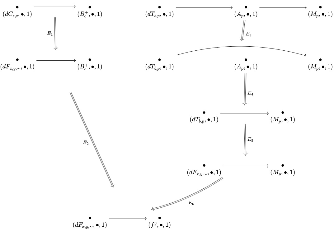
Figure 3.

In Figure 3, $E_{1},E_{2},E_{5},E_{6}$ are all operations of type (v) in the sense of Section LABEL:sec:distanceedit-WD, i.e. each of them is just a change of a single label; in all these instances, we are changing a label to a more abstract label. The operation $E_{3}$ is of type (viii) - it corresponds to an irreducible morphism in the category $\mathcal{R}(V)$ where $V$ is the set of vertices in $W_{2}$. The operation $E_{4}$ is of type (ii), where the vertex with a single label $(A_{p},\bullet,1)$ is deleted. If write $E_{i}^{-1}$ for the inverse of an elementary edit operation $E^{i}$, then each $E_{i}$ is again an elementary edit operation and $W_{1}$ is transformed into $W_{2}$ via the sequence of operations

$$(E_{1},E_{2},E_{6}^{-1},E_{5}^{-1},E_{4}^{-1},E_{3}^{-1}).$$

Now for any cost function $c:\mathrm{EEO}(W_{s}^{\bullet})\to\mathbb{R}_{>0}$, we obtain an upper bound for the distance $d(W_{1},W_{2})$ using the metric $d$ from Lemma 6.8:

$$d(W_{1},W_{2})\leq\sum_{i=1}^{2}c(E_{i})+\sum_{i=3}^{6}c(E_{i}^{-1}).$$

7.3.2 L

et us use $W_{1}^{\prime}$ and $W_{2}^{\prime}$ as representations of $S_{1}$ and $S_{2}$, respectively. In this case, no wiring diagram labels are defined using numerical derivatives of sensing functions, and $W_{1}^{\prime}$ and $W_{2}^{\prime}$ are related via elementary edit operations as shown in Figure 4. We will also make use of the ologs in (7.2.1) and (7.2.2) more directly in defining our cost function $c$ for the metric on $W_{s}^{\bullet}$.

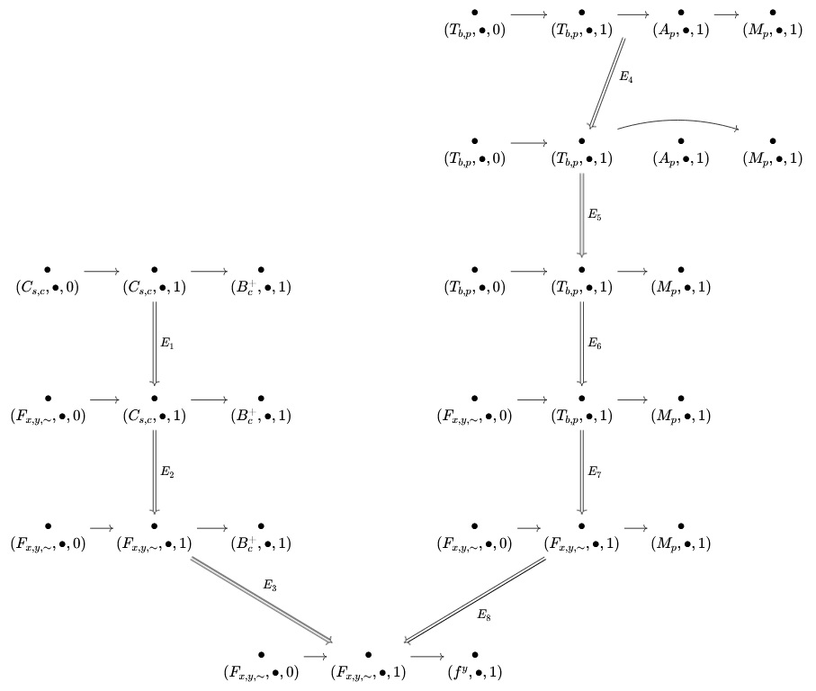
Figure 4.

In Figure 4, the operation $E_{4}$ is of type (viii) while $E_{5}$ is of type (ii). On the other hand, the operations $E_{1},E_{2},E_{3},E_{6},E_{7},E_{8}$ are all of type (v); each of these six operations involves changing the sensing function in a label to a different sensing function. For example, $E_{1}$ involves changing $(C_{s,c},\bullet,0)$ to $(F_{x,y,\thicksim},\bullet,0)$, while $E_{3}$ involves changing $(B_{c}^{+},\bullet,1)$ to $(f^{y},\bullet,1)$. Note that all the labels involving $C_{s,c},B_{c}^{+},F_{x,y,\thicksim},f^{y}$ in Figure 4 are represented by types in the ologs in (7.2.1) and (7.2.2):

Label	Type
$(C_{s,c},\bullet,0)$	$G_{0}$
$(C_{s,c},\bullet,1)$	$G_{1}$
$(B_{c}^{+},\bullet,1)$	$A_{1}$
$(F_{x,y,\thicksim},\bullet,0)$	$T_{0}$
$(f^{y},\bullet,1)$	$P_{1}$

Using constructions similar to those in (7.2.1) and (7.2.2), we could expand these ologs to contain types corresponding to all the other labels in Figure 4, too. Combining these ologs into a single olog $O$, then choosing a cost function $c_{O}$ on the edges underlying $O$ and proceeding as in Example 6.8, we obtain a metric $d$ on $W_{s}^{\bullet}$ that utilizes the ologs in (7.2.1) and (7.2.2) in calculating $d(W_{1}^{\prime},W_{2}^{\prime})$. From Figure 4, we now have the upper bound for $d(W_{1}^{\prime},W_{2}^{\prime})$

$$d(W_{1}^{\prime},W_{2}^{\prime})\leq\sum_{i=1}^{3}c(E_{i})+\sum_{i=4}^{8}c(E_{i}^{-1}).$$

Remark 7.4.

• Whether we take Approach 1 or Approach 2 above, the actual distance between the two wiring diagrams being compared would depend on the olog being used to represent all the relevant concepts and the specific elementary edit operations allowed. For example, in Approach 1, if we had allowed an arbitrary change of label in elementary edit operations of type (v), then there would be such an operation connecting the second diagram in the left column and the third diagram in the right column in Figure 3. The specific elementary edit operations of type (v) used in Figures 3 and 4 make the point, that the two concepts we are trying to connect (‘electric car charging station’ and ‘bus’) can both be connected to a more abstract concept (represented by the wiring diagram at the bottom in either Figure 3 or Figure 4). In particular, the operation $E_{3}$ in Figure 3 and the operation $E_{4}$ in Figure 4, both of which are morphisms in some category $\mathcal{R}(V)$, make mathematically precise what it means for a concept to be “more abstract” than another.

• One could argue that, strictly speaking, some of the wiring diagrams in Figures 3 and 4 do not satisfy our definition of wiring diagrams (Definition 2) because, in WD1, we require that the first argument of every vertex label be a specific sensing function, whereas entries such as $dF_{x,y,\thicksim}$ and $f^{y}$ in Figures 3 and 4 are ‘generic’ sensing functions. We can get around this technical issue by extending the definition of wiring diagrams and allowing the arguments of vertex labels to be types in an olog. This will be explored in a sequel to this article.

7.5

para:summaryofcalc We now give a summary of the steps that one can follow in order to compute the distance between pairs of concepts in a given application domain. Suppose the concepts we are concerned with are elements of an indexed set $\{N_{i}\}_{i\in I}$. Then one can perform the following tasks in the listed order:

1. Define the relevant sensing functions.

2. Define wiring diagrams $W_{i}$ that represent the concepts $N_{i}$.

3. Construct an olog (or ologs) containing types that correspond to all the labels in the wiring diagrams $W_{i}$ (e.g. see LABEL:sec:WDandologs and LABEL:sec:relnsfs).

4. Decide on a list of acceptable elementary edit operations on wiring diagrams. For example, one may wish to restrict the kinds of allowed operations of type (v) in the list in LABEL:sec:distanceedit-WD.

5. Decide on a cost function $c$ in the definition of the metric on wiring diagrams in Lemma 6.8. More specifically, one needs to decide on the cost of each elementary edit operation, such as the cost of an operation of type (v) - see Example 6.8.

6. For any two distinct concepts $N_{i},N_{j}$, calculate their distance $d(N_{i},N_{j})$ using the definition in Lemma 6.8. Each possible edit path from $N_{i}$ to $N_{j}$ would constitute a ‘justification’, or a mathematical breakdown of the analogy between concept $N_{i}$ and concept $N_{j}$.

For the main example in this section, Steps (1) and (2) were implemented in LABEL:para:steps-sf, Steps (3) was implemented in LABEL:para:eg-step2-ologs, while Steps (4) through (6) were implemented in LABEL:para:steps-eeo.

8. Future directions

In this article, we first recalled how ologs can be used to represent abstract concepts. Then we define the concept of wiring diagrams where labels at vertices correspond to types in an olog. Wiring diagrams allow us to represent concepts corresponding to temporal processes, which may not be so easily represented using ologs alone. We can think of wiring diagrams as giving a coordinate system, or a state space on which one can develop a theory of problem-solving. This direction will be explored in a sequel to this article.

As mentioned in LABEL:para:intro-WD, the term ‘wiring diagram’ has also been defined and studied as operads in works such as [15, 17, 21, 25]. The wiring diagrams as defined in this article certain show features of self-similarity - under appropriate assumptions, one can replace any vertex in a wiring diagram (along with its state vector) by a wiring diagram to obtain a more complicated wiring diagram. It would be worthwhile to reconcile the definition of wiring diagrams in this article with those in the aforementioned works. In the present article, we refrained from doing so in order to keep our theory accessible to a wider audience.

Example 5.10 hinted at the complexity that can be encoded within the underlying graphs of wiring diagrams. For example, a wiring diagram of the form (5.12.2) may be an indication of the social behavior of collaboration. This opens up a host of questions to be answered. For example, given a sequence of events over time, what are the possible wiring diagrams that possess these events as the state vectors, and how many are there? Mathematically, this is related to the problem of enumerating all the preorders or partial orders on a set of given objects, and perhaps related to the notion of graph fibrations [2]. One can also ask if wiring diagrams can be used to classify behaviors, whether in the context of biology (behaviors of different species), social science (behaviors of humans or organizations), finance (behaviors of markets).

Lastly, the definition of wiring diagrams we adopted in this paper applies to any type of data that admits a fibration into a linearly ordered set - the concept of ordering among the state vectors in a wiring diagram comes from condition WD2 in Definition 2. In all the wiring diagrams we considered in this paper, the state vectors always corresponded to events that can be partially ordered with respect to time (i.e. whether one event is required to occur before another). Nonetheless, one can just as well consider wiring diagrams where the ordering is given by causation, for example, as in the case of mathematical proofs. As shown in examples in [20, Sections 6.6-6.7] (see also [10]), some mathematical definitions can be expressed via ologs, after which mathematical lemmas can be expressed as commutativity of diagrams within the olog. One could potentially think of a mathematical proof as a wiring diagram where the state vectors correspond to various ‘milestones’ in the proof, and where arrows are defined using causation among the milestones. One could then make precise what we mean when we say two mathematical proofs are ‘similar’, or that the argument of one proof in a specific context ‘carries over’ in a different context.

References

- [1] Steve Awodey. Category Theory. Oxford University Press, Inc., USA, 2nd edition, 2010.
- [2] Paolo Boldi and Sebastiano Vigna. Fibrations of graphs. Discrete Mathematics, 243(1-3):21–66, 2002.
- [3] Dieter B Brommer, Tristan Giesa, David I Spivak, and Markus J Buehler. Categorical prototyping: Incorporating molecular mechanisms into 3d printing. Nanotechnology, 27(2):024002, 2015.
- [4] Aleksandr Drozd, Anna Gladkova, and Satoshi Matsuoka. Word embeddings, analogies, and machine learning: Beyond king - man + woman = queen. In Yuji Matsumoto and Rashmi Prasad, editors, Proceedings of COLING 2016, the 26th International Conference on Computational Linguistics: Technical Papers, pages 3519–3530, Osaka, Japan, December 2016. The COLING 2016 Organizing Committee.
- [5] X. Gao, B. Xiao, D. Tao, and X. Li. A survey of graph edit distance. Pattern Analysis and Applications, 13:113–129, 2010.
- [6] Tristan Giesa, David I Spivak, and Markus J Buehler. Category theory based solution for the building block replacement problem in materials design. Advanced Engineering Materials, 14(9):810–817, 2012.
- [7] Jonathan L. Gross, Jay Yellen, and Ping Zhang. Handbook of Graph Theory, Second Edition. Chapman & Hall/CRC, 2nd edition, 2013.
- [8] Daniel C. Krawczyk. Chapter 10 - analogical reasoning. In Daniel C. Krawczyk, editor, Reasoning, pages 227–253. Academic Press, 2018.
- [9] Saunders MacLane. Categories for the Working Mathematician. Springer-Verlag, New York, 1971. Graduate Texts in Mathematics, Vol. 5.
- [10] P. Mavromichalis. Proofs in group theory in the context of ologs, 2023. Master’s thesis at California State University, Northridge.
- [11] Michel Neuhaus and Horst Bunke. Bridging the Gap Between Graph Edit Distance and Kernel Machines. World Scientific Publishing Co., Inc., USA, 2007.
- [12] M. A. Pérez and D. I. Spivak. Toward formalizing ologs: linguistic structures, instantiations, and mappings. Preprint. arXiv:1503.08326 [math.CT], 2015.
- [13] Molly Petersen and Lonneke van der Plas. Can language models learn analogical reasoning? investigating training objectives and comparisons to human performance. In Houda Bouamor, Juan Pino, and Kalika Bali, editors, Proceedings of the 2023 Conference on Empirical Methods in Natural Language Processing, pages 16414–16425, Singapore, December 2023. Association for Computational Linguistics.
- [14] K. Riesen and H. Bunke. Graph Classification and Clustering Based on Vector Space Embedding. Series in Machine Perception and Artificial Intelligence. World Scientific, Singapore, 2010.
- [15] D. Rupel and D. I. Spivak. The operad of temporal wiring diagrams: formalizing a graphical language for discrete-time processes. Preprint. arXiv:1307.6894 [math.CT], 2013.
- [16] F. Serratosa. Redefining the graph edit distance. SN Computer Science, 2(438), 2021.
- [17] D. I. Spivak. The operad of wiring diagrams: formalizing a graphical language for databases, recursion, and plug-and-play circuits. 2013.
- [18] David I. Spivak. Category Theory for the Sciences. The MIT Press, 2014.
- [19] David I Spivak, Tristan Giesa, Elizabeth Wood, and Markus J Buehler. Category theoretic analysis of hierarchical protein materials and social networks. PloS one, 6(9):e23911, 2011.
- [20] David I. Spivak and Robert E. Kent. Ologs: A categorical framework for knowledge representation. PLOS ONE, 7(1), 01 2012.
- [21] D. Vagner, D. I. Spivak, and E. Lerman. Algebras of open dynamical systems on the operad of wiring diagrams. Theory and Applications of Categories, 30(51):1793–1822, 2015.
- [22] R. F. C. Walters. Categories and Computer Science. Cambridge Computer Science Texts. Cambridge University Press, 1992.
- [23] Peter Wills and François G Meyer. Metrics for graph comparison: a practitioner’s guide. Plos one, 15(2):e0228728, 2020.
- [24] Y. Wu. Gene ologs: a categorical framework for gene ontology. Preprint. arXiv:1909.11210 [q-bio.GN], 2019.
- [25] Donald Yau. Operads of wiring diagrams, volume 2192. Springer, 2018.