Multivariate Probabilistic Time Series Forecasting with Correlated Errors

Abstract

Modeling the correlations among errors is closely associated with how accurately the model can quantify predictive uncertainty in probabilistic time series forecasting. Recent multivariate models have made significant progress in accounting for contemporaneous correlations among errors, while a common assumption on these errors is that they are temporally independent for the sake of statistical simplicity. However, real-world observations often deviate from this assumption, since errors usually exhibit substantial autocorrelation due to various factors such as the exclusion of temporally correlated covariates. In this work, we propose an efficient method, based on a low-rank-plus-diagonal parameterization of the covariance matrix, which can effectively characterize the autocorrelation of errors. The proposed method possesses several desirable properties: the complexity does not scale with the number of time series, the resulting covariance can be used for calibrating predictions, and it can seamlessly integrate with any model with Gaussian-distributed errors. We empirically demonstrate these properties using two distinct neural forecasting models—GPVar and Transformer. Our experimental results confirm the effectiveness of our method in enhancing predictive accuracy and the quality of uncertainty quantification on multiple real-world datasets.

1 Introduction

Uncertainty quantification plays a crucial role in time series forecasting, particularly for downstream applications that require more nuanced insights than simple point forecasts to guide decision making. Probabilistic time series forecasting based on deep learning (DL) has gained substantial attention in recent years, due to its outstanding performance in capturing complex and nonlinear dependencies in time series data and its ability to provide the probability distribution of target variables (Benidis et al., 2022). For multivariate time series, recent neural network models (Salinas et al., 2019; Rasul et al., 2020, 2021; Drouin et al., 2022; Ashok et al., 2023) are typically framed as a regression problem $\mathbf{z}_{t}=f\left(\mathbf{x}_{t}\right)+\boldsymbol{\eta}_{t}$. In a simple scenario, the error term $\boldsymbol{\eta}_{t}$ follows a Gaussian distribution $\mathcal{N}(\mathbf{0},\boldsymbol{\Sigma}_{t})$, where $\boldsymbol{\Sigma}_{t}$ is the contemporaneous covariance matrix. A common assumption in these models is that errors are independent over time, which means $\operatorname{Cov}(\boldsymbol{\eta}_{s},\boldsymbol{\eta}_{t})=\mathbf{0}$ for any times $s$ and $t$ such that $s\neq t$. However, real-world data rarely conforms to this assumption—errors often exhibit a certain degree of autocorrelation due to factors such as the omission of essential covariates.

Addressing error autocorrelation is a crucial aspect of research in classical time series models. A common strategy in this regard is dynamic regression, which assumes that the error series follows a temporal process, such as an autoregressive integrated moving average (ARIMA) model (Hyndman & Athanasopoulos, 2018). The similar challenge also arises in deep learning models. Previous studies have sought to integrate autocorrelated errors into the training process through modifying the loss function (Sun et al., 2021; Zheng et al., 2023b). However, the aforementioned methods, which are based on deterministic output, are not readily applicable to probabilistic forecasting models, particularly in the multivariate setting. A notable exception to address error autocorrelation in univariate time series is the innovative batch training method proposed by Zheng et al. (2023a), which learns a dynamic covariance matrix of time-assorted errors in a mini-batch. The covariance matrix can then be used to calibrate the predictive distribution of time series variables. It is shown that the method can consistently enhance the performance of base probabilistic models when compared to the naive training approach (i.e., without considering autocorrelated errors). However, the approach of Zheng et al. (2023a) is only applicable to univariate probabilistic time series forecasting models (e.g., DeepAR (Salinas et al., 2020)).

In this paper, we extend the method introduced by Zheng et al. (2023a) to multivariate probabilistic time series forecasting. The immediate challenge of modeling error autocorrelation in multivariate models lies in the increased dimensionality. Specifically, the size of the covariance matrix for modeling autocorrelation will be scaled by $N$, the number of time series. To address this issue, we propose an efficient method to explicitly characterize the serial correlation in errors by combining a low-rank parameterization of the covariance matrix with a group of independent latent temporal processes. This approach also solves the problem where the computational cost scales with the number of time series in a mini-batch. Our work results in a general-purpose approach to multivariate probabilistic time series models, which offers significantly improved predictive accuracy.

Contributions:

1. We introduce an efficient method to train multivariate probabilistic time series forecasting models with autocorrelated errors (§4).

2. We propose an efficient parameterization to learn dynamic covariance matrices, for which the inverse and determinant can be efficiently computed using the matrix inversion lemma and the matrix determinant lemma (§4.1).

3. The covariance matrix can be used to fine-tune the predictive distribution based on observed residuals (§4.2).

4. We demonstrate that the proposed method can effectively capture error autocorrelation and enhance prediction quality. Notably, these enhancements are achieved through a statistical formulation without a significant increase in the size of model parameters. (§5).

2 Probabilistic Time Series Forecasting

Denote $\mathbf{z}_{t}=\left[z_{1,t},\dots,z_{N,t}\right]^{\top}\in\mathbb{R}^{N}$ as the vector containing the time series variables at time step $t$, where $N$ is the number of time series. Probabilistic time series forecasting can be formulated as estimating the joint conditional distribution $p\left(\mathbf{z}_{{T+1}:{T+Q}}\mid\mathbf{z}_{{T-P+1}:{T}};\mathbf{x}_{{T-P+1}:{T+Q}}\right)$ based on the observed history $\{\mathbf{z}_{t}\}_{t=1}^{T}$, where $\mathbf{z}_{{t_{1}}:{t_{2}}}=\left[\mathbf{z}_{t_{1}},\ldots,\mathbf{z}_{t_{2}}\right]$ and $\mathbf{x}_{t}$ is the vector containing known covariates (e.g., time information and time series identifiers) for all time steps. In essence, the problem can be described as predicting the time series values for $Q$ future time steps, using all available covariates and $P$ steps of historical time series values:

$$p\left(\mathbf{z}_{{T+1}:{T+Q}}\mid\mathbf{z}_{{T-P+1}:{T}};\mathbf{x}_{{T-P+1}:{T+Q}}\right)\\ =\prod_{t=T+1}^{T+Q}p\left(\mathbf{z}_{t}\mid\mathbf{z}_{{t-P}:{t-1}};\mathbf{x}_{{t-P}:{t}}\right),$$ (1)

which results in an autoregressive model that is capable of multi-step forecasting in a rolling manner. When performing multi-step forecasting, samples will be drawn in the prediction range ($t\geq T+1$) and fed back for the next time step until the end of the desired prediction range. In neural networks, the conditioning information is typically integrated into a hidden state vector $\mathbf{h}_{t}$ governed by a transition dynamics $f_{\Theta}$ evolving over time $\mathbf{h}_{t}=f_{\Theta}\left(\mathbf{h}_{t-1},\mathbf{z}_{t-1},\mathbf{x}_{t}\right)$. Hence, Eq. (1) can be expressed more concisely:

$$p\left(\mathbf{z}_{{T+1}:{T+Q}}\mid\mathbf{z}_{{T-P+1}:{T}};\mathbf{x}_{{T-P+1}:{T+Q}}\right)\\ =\prod_{t=T+1}^{T+Q}p\left(\mathbf{z}_{t}\mid\mathbf{h}_{t}\right),$$ (2)

where $\mathbf{h}_{t}$ is used for generating the parameters of a parametric distribution (e.g., multivariate Gaussian).

Existing models usually assume that the error at each time step is independent, and thus the time series vector $\mathbf{z}_{t}$ follows a multivariate Gaussian distribution:

$$\left.\mathbf{z}_{t}\mid\mathbf{h}_{t}\right.\sim\mathcal{N}\left(\boldsymbol{\mu}(\mathbf{h}_{t}),\boldsymbol{\Sigma}(\mathbf{h}_{t})\right),$$ (3)

where $\boldsymbol{\mu}(\cdot)$ and $\boldsymbol{\Sigma}(\cdot)$ map the hidden state $\mathbf{h}_{t}$ to the mean and covariance of a multivariate Gaussian distribution. This formulation is equivalent to decomposing $\mathbf{z}_{t}=\boldsymbol{\mu}_{t}+\boldsymbol{\eta}_{t}$ with $\boldsymbol{\eta}_{t}\sim\mathcal{N}(\mathbf{0},\boldsymbol{\Sigma}_{t})$. The temporally independent error assumption corresponds to $\operatorname{Cov}(\boldsymbol{\eta}_{s},\boldsymbol{\eta}_{t})=\mathbf{0}$ for any time points $s$ and $t$ such that $s\neq t$. Fig. 1 provides an empirical example of the contemporaneous covariance matrix $\operatorname{Cov}(\boldsymbol{\eta}_{t},\boldsymbol{\eta}_{t})$ and cross-covariance matrix $\operatorname{Cov}(\boldsymbol{\eta}_{t-\Delta},\boldsymbol{\eta}_{t}),\Delta=1,2,3$. The results are calculated based on the prediction residuals of GPVar on the $\mathtt{m4\_hourly}$ dataset. While multivariate models primarily focus on modeling the contemporaneous covariance, it is evident that the residuals are not independent across time, as $\operatorname{Cov}(\boldsymbol{\eta}_{t-\Delta},\boldsymbol{\eta}_{t})\neq\mathbf{0}$.

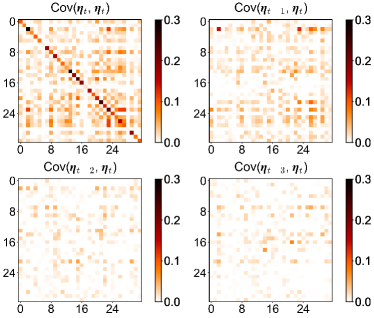
Figure 1: Contemporaneous covariance matrix $\operatorname{Cov}(\boldsymbol{\eta}_{t},\boldsymbol{\eta}_{t})$ and cross-covariance matrix $\operatorname{Cov}(\boldsymbol{\eta}_{t-\Delta},\boldsymbol{\eta}_{t}),\Delta=1,2,3$, calculated based on the one-step-ahead prediction residuals of GPVar on a batch of time series from the $\mathtt{m4\_hourly}$ dataset. To enhance the clarity of the visualization, covariance values are clipped to the range of 0 and 0.3.

3 Related Work

3.1 Probabilistic Time Series Forecasting

Probabilistic forecasting quantifies uncertainty by characterizing the probability distribution for the target variable(s). There are two primary approaches to achieve this objective. One approach involves using the quantile function. For example, the MQ-RNN (Wen et al., 2017) directly generates quantile forecasts through a sequence-to-sequence (Seq2Seq) recurrent neural network (RNN) architecture. Another approach is based on probability density functions (PDF) of the target variables. PDF-based approaches assume a specific probabilistic models (e.g., Gaussian processes) for the target variables and utilize neural networks to generate the parameters of these probabilistic models. Notably, DeepAR (Salinas et al., 2020) utilizes an RNN architecture to model hidden state transitions. The multivariate version of DeepAR—GPVar (Salinas et al., 2019)—utilizes a Gaussian copula to transform the original observations into Gaussian random variables. Subsequently, the model assumes a joint multivariate Gaussian distribution on the transformed data.

In addition to outputting distribution parameters, neural networks can be used to generate probabilistic model parameters, as exemplified by the deep state space model (SSM) (Rangapuram et al., 2018), which uses RNN to generate SSM parameters for predicting samples. The Normalizing Kalman Filter (NKF), introduced by (de Bézenac et al., 2020), integrates normalizing flows (NFs) with the classical Linear Gaussian State Space Model (LGM) to capture nonlinear dynamics and assess the probability density function of observations. In NKF, RNN is used to produce parameters for the LGM at each time step. Subsequently, the output of the LGM is transformed into the observations using NFs. Wang et al. (2019) proposed the deep factor model that is comporised of a deterministic global component and a random component. The global component is parameterized by RNN for generating the global factors of time series, while the random component is any classical probabilistic time series model (e.g., Gaussian white noise process) for representing random effects.

Some approaches focus on improving expressive conditioning for probabilistic forecasting, such as using Transformer instead of RNN to model latent state dynamics, thus breaking the Markovian assumption in RNN (Tang & Matteson, 2021). Another avenue to improve probabilistic forecasting involves adopting more flexible distribution forms, including normalizing flows (Rasul et al., 2020), diffusion models (Rasul et al., 2021), and Copula (Drouin et al., 2022; Ashok et al., 2023). We refer readers to Benidis et al. (2022) for a recent and comprehensive review.

3.2 Modeling Correlated Errors

Error correlation in time series is an extensively explored subject in the fields of econometrics and statistics (Prado et al., 2021; Hyndman & Athanasopoulos, 2018; Hamilton, 2020). Autocorrelation, or serial correlation, and contemporaneous correlation are two primary types of correlation. Autocorrelation refers to the temporal correlation of errors in a time series, while contemporaneous correlation captures the correlation among variables within the same time period. Classical statistical frameworks, including autoregressive (AR) and moving average (MA) models, along with their multivariate counterparts, have been firmly established to address these correlation challenges. Recent developments in DL-based time series models have also sought to explicitly model error correlation structures to enhance forecasting performance.

For example, Sun et al. (2021) re-parameterize the input and output of a neural network to model first-order error autocorrelation in time series, effectively capturing serially correlated errors with an AR$(1)$ process. This approach improves the performance of DL-based one-step-ahead forecasting models, enabling joint optimization of the base and error regressors. This methodology is extended to multivariate models for Seq2Seq time series forecasting tasks, assuming a matrix autoregressive (AR) process for the error matrix (Zheng et al., 2023b).

To address contemporaneous correlation, researchers have proposed modeling error correlation using a multivariate Gaussian distribution in node regression problems (Jia & Benson, 2020). The resulting method, known as error propagation in graph neural networks (GNNs), adjusts the prediction of unknown nodes based on known node labels. The generalized least squares (GLS) loss, introduced by Zhan & Datta (2023), captures spatial correlation of errors in neural networks for geospatial data, bridging the gap between deep learning and Gaussian processes. This GLS approach can also be integrated into other nonlinear regression models, such as random forest (Saha et al., 2023).

In the work of Choi et al. (2022), a dynamic mixture of matrix Gaussian distributions was proposed to characterize spatiotemporally-correlated errors in Seq2Seq models. Additionally, Zheng et al. (2023a) introduced a dynamic covariance matrix for modeling autocorrelated errors in univariate probabilistic time series forecasting using a re-organized training batch.

4 Our Method

Our methodology builds upon the formulation outlined in Eq. (2), employing an autoregressive model as its foundational framework. Broadly speaking, an autoregressive probabilistic forecasting model consists of two fundamental components. Firstly, it incorporates a transition model, such as an RNN, to capture the dynamics of state transitions denoted by $\mathbf{h}_{t}$. Secondly, it integrates a distribution head, represented by $\theta$, which is tasked with mapping the state representation $\mathbf{h}_{t}$ to the parameters governing the desired probability distribution. Following the GPVar model (Salinas et al., 2019), our approach employs the multivariate Gaussian distribution as the distribution head. The parameters $\theta(\mathbf{h}_{t})$ are parameterized as $(\boldsymbol{\mu}_{t},\boldsymbol{L}_{t},\mathbf{d}_{t})$, where $\boldsymbol{\mu}_{t}\in\mathbb{R}^{N}$ represents the mean vector of the distribution. $\boldsymbol{L}_{t}\in\mathbb{R}^{N\times R}$ and $\mathbf{d}_{t}\in\mathbb{R}^{N}$ correspond to the covariance factor and diagonal elements in the low-rank parameterization of the multivariate Gaussian distribution. We use shared mapping functions for all time series:

$$\mu_{i}(\mathbf{h}_{i,t}) =\tilde{\mu}(\mathbf{h}_{i,t})=\mathbf{w}_{\mu}^{\top}\mathbf{h}_{i,t},$$ (4)

$$d_{i}(\mathbf{h}_{i,t}) =\tilde{d}(\mathbf{h}_{i,t})=\log(1+\exp(\mathbf{w}_{d}^{\top}\mathbf{h}_{i,t})),$$

$$\ l_{i}(\mathbf{h}_{i,t}) =\tilde{l}(\mathbf{h}_{i,t})=W_{l}\mathbf{h}_{i,t},$$

where $\mathbf{h}_{i,t}\in\mathbb{R}^{H\times 1}$, $\mathbf{w}_{\mu}\in\mathbb{R}^{H\times 1}$, $\mathbf{w}_{d}\in\mathbb{R}^{H\times 1}$, and $W_{l}\in\mathbb{R}^{R\times H}$ are parameters. This parameterization allows us to view $\mathbf{z}_{t}$ as a Gaussian process assessed at points $\mathbf{h}_{i,t}$. Consequently, we can leverage a random subset of time series to compute the Gaussian likelihood-based loss in each iteration. In other words, we can train the model with a substantially reduced batch size $B\leq N$.

In the training batch, the target time series vector can be decomposed into a deterministic mean component and a random error component:

$$\mathbf{z}_{t}=\boldsymbol{\mu}_{t}+\boldsymbol{\eta}_{t},$$ (5)

where $\boldsymbol{\eta}_{t}\sim\mathcal{N}(\mathbf{0},\boldsymbol{\Sigma}_{t})$. To efficiently model covariance $\boldsymbol{\Sigma}_{t}$ for large $N$, GPVar adopts a low-rank plus diagonal parameterization $\boldsymbol{\Sigma}_{t}=\boldsymbol{L}_{t}\boldsymbol{L}_{t}^{\top}+\operatorname{diag}{(\mathbf{d}_{t})}$, where $\boldsymbol{L}_{t}\in\mathbb{R}^{N\times R}$ ($R\ll N)$ and $\boldsymbol{d}_{t}\in\mathbb{R}_{+}^{N}$.

Models based on Gaussian likelihood are usually built on the assumption that $\boldsymbol{\eta}_{t}$ are independently distributed and following a multivariate Gaussian distribution. The log-likelihood of the distribution serves as the loss function for optimizing the model:

$$\mathcal{L}=\sum_{t=1}^{T}\log p\left(\mathbf{z}_{t}\mid\theta\left(\mathbf{h}_{t}\right)\right)\propto\sum_{t=1}^{T}-\frac{1}{2}[\ln\lvert\boldsymbol{\Sigma}_{t}\rvert+\boldsymbol{\eta}_{t}^{\top}\boldsymbol{\Sigma}_{t}^{-1}\boldsymbol{\eta}_{t}].$$ (6)

4.1 Training with Autocorrelated Errors

Building upon the concept of constructing mini-batches to address autocorrelated errors (Zheng et al., 2023a), we extend this approach to the multivariate scenario. In many existing deep probabilistic time series models, including GPVar (Salinas et al., 2019), each training batch encompasses a set of time series slices covering a temporal length of $P+Q$, where $P$ represents the conditioning range, and $Q$ denotes the prediction range. Gaussian likelihood is assessed individually at each time step within the prediction range. However, this simple approach does not account for the serial correlation of errors between successive time steps. To address this limitation, we organize $D$ consecutive batches into a mini-batch, with each batch covering a temporal length of $P+1$ (i.e., $Q=1$). In simpler terms, a traditional training batch comprises data $\mathbf{z}_{{T-P+1}:{T+Q}}$, while a mini-batch consists of data $\{\mathbf{z}_{{T-P+t}:{T+t}}\}_{t=1}^{D}$, where $T$ denotes a randomly sampled time step that separates the conditioning range and prediction range. It is evident that the mini-batch serves as a reconstruction of the conventional training batch, covering the same time horizon if $D=Q$. An example of the collection of target time series vectors in a mini-batch of size $D$ (the time horizon we use to capture serial correlation) is given by:

$$\mathbf{z}_{t} =\boldsymbol{\mu}_{t}+\boldsymbol{\eta}_{t},$$ (7)

$$\mathbf{z}_{t+1} =\boldsymbol{\mu}_{t+1}+\boldsymbol{\eta}_{t+1},$$

$$\ldots$$

$$\mathbf{z}_{t+D-1} =\boldsymbol{\mu}_{t+D-1}+\boldsymbol{\eta}_{t+D-1},$$

where for time point $t^{\prime}$, $\boldsymbol{\mu}_{t^{\prime}}$, $\boldsymbol{L}_{t^{\prime}}$ and $\mathbf{d}_{t^{\prime}}$ are the output of the model. The covariance parameterization in GPVar corresponds to

$$\boldsymbol{\eta}_{t^{\prime}}=\boldsymbol{L}_{t^{\prime}}\mathbf{r}_{t^{\prime}}+\boldsymbol{\varepsilon}_{t^{\prime}},$$ (8)

where $\mathbf{r}_{t^{\prime}}\sim\mathcal{N}(\mathbf{0},\mathbf{I}_{R})$ is a low-dimensional latent variable, and $\boldsymbol{\varepsilon}_{t^{\prime}}\sim\mathcal{N}(\mathbf{0},\operatorname{diag}{(\mathbf{d}_{t^{\prime}})})$ is an additional error that is independent of $\mathbf{r}_{t^{\prime}}$. We denote by $\boldsymbol{z}_{t}^{\text{bat}}=\operatorname{vec}\left(\mathbf{z}_{t:t+D-1}\right)\in\mathbb{R}^{DB}$ the collection of target time series vectors in a mini-batch, where $\operatorname{vec}(\cdot)$ is an operator that stacks all the columns of a matrix into a vector. Similarly, we have $\boldsymbol{\mu}_{t}^{\text{bat}}\in\mathbb{R}^{DB}$, $\boldsymbol{r}_{t}^{\text{bat}}\in\mathbb{R}^{DR}$, $\boldsymbol{\varepsilon}_{t}^{\text{bat}}\in\mathbb{R}^{DB}$, $\boldsymbol{d}_{t}^{\text{bat}}\in\mathbb{R}^{DB}$, and $\boldsymbol{L}_{t}^{\text{bat}}=\operatorname{blkdiag}(\{\boldsymbol{L}_{t^{\prime}}\}_{t^{\prime}=t}^{t+D-1})\in\mathbb{R}^{DB\times DR}$ (Fig. 2). We can then write the batch-wise decomposition as:

$$\boldsymbol{z}_{t}^{\text{bat}}=\boldsymbol{\mu}_{t}^{\text{bat}}+\boldsymbol{L}_{t}^{\text{bat}}\boldsymbol{r}_{t}^{\text{bat}}+\boldsymbol{\varepsilon}_{t}^{\text{bat}}.$$ (9)

The default GPVar model assumes the latent variable $\boldsymbol{r}$ to be temporally independent, i.e., $\operatorname{Cov}\left(\boldsymbol{r}_{t},\boldsymbol{r}_{t^{\prime}}\right)=\boldsymbol{0},\forall t\neq t^{\prime}$. However, this assumption cannot accommodate the potential autocorrelation in the error. We next introduce temporal dependency in the latent variable in a mini-batch by assuming $\boldsymbol{r}_{t}^{\text{bat}}\sim\mathcal{N}\left(\boldsymbol{0},\boldsymbol{C}_{t}\otimes\mathbf{I}_{R}\right)$, where $\boldsymbol{C}_{t}$ is a $D\times D$ dynamic correlation matrix. This approach corresponds to assuming that the rows in the matrix $\mathbf{r}_{t:t+D-1}=\left[\mathbf{r}_{t},\ldots,\mathbf{r}_{t+D-1}\right]$ are independent and identically distributed following $\mathcal{N}\left(\boldsymbol{0},\boldsymbol{C}_{t}\right)$. To efficiently capture dynamic patterns over time, we follow Zheng et al. (2023b) and express $\boldsymbol{C}_{t}$ as a dynamic weighted sum of those base kernel matrices: $\boldsymbol{C}_{t}=\sum_{m=1}^{M}w_{m,t}\boldsymbol{K}_{m}$, where $w_{m,t}\geq 0$ (with $\sum_{m}w_{m,t}=1$) represents the weights for each component. For simplicity, we model each component $\boldsymbol{K}_{m}$ using a kernel matrix generated from a squared-exponential (SE) kernel function, with the $(i,j)$th entry being $\boldsymbol{K}^{ij}_{m}=\exp(-\frac{(i-j)^{2}}{l_{m}^{2}})$, with different lengthscales $l$ (e.g., $l=1,2,3,\dots$). In addition, we incorporate an identity matrix into the additive structure to account for the independent noise process. This parameterization ensures that $\boldsymbol{C}_{t}$ is a positive definite symmetric matrix with unit diagonals, making it a valid correlation matrix. The weights for these components are derived from the hidden state $\mathbf{h}_{t}$ at each time step through a small neural network, with the number of nodes in the output layer set to $M$ (i.e., the number of components). A softmax layer is then used to ensure that these weights are summed up to 1. Note that the parameters of this network will be learned simultaneously with those of the base model.

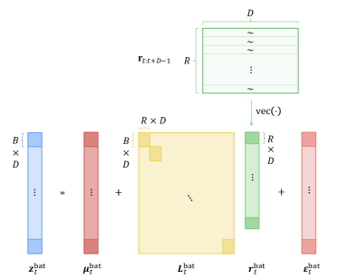
Figure 2: Graphic illustration of Eq. (9). Autocorrelation is modeled by introducing correlation in each row of matrix $\mathbf{r}_{t:t+D-1}$.

Marginalizing out $\boldsymbol{r}_{t}^{\text{bat}}$ in Eq. (9), we have $\boldsymbol{z}_{t}^{\text{bat}}\sim\mathcal{N}\left(\boldsymbol{\mu}_{t}^{\text{bat}},\boldsymbol{\Sigma}_{t}^{\text{bat}}\right)$ with covariance

$$\boldsymbol{\Sigma}_{t}^{\text{bat}}=(\boldsymbol{L}_{t}^{\text{bat}})(\boldsymbol{C}_{t}\otimes\mathbf{I}_{R})(\boldsymbol{L}_{t}^{\text{bat}})^{\top}+\operatorname{diag}(\boldsymbol{d}_{t}^{\text{bat}}).$$ (10)

It is not difficult to derive that for any $i,j\in\{0,1,\ldots,D-1\}$ and $i\neq j$, the proposed model can create cross-covariance $\operatorname{Cov}\left(\boldsymbol{\eta}_{t+i},\boldsymbol{\eta}_{t+j}\right)=\boldsymbol{C}_{t}^{ij}\boldsymbol{L}_{t+i}\boldsymbol{L}_{t+j}^{\top}$ for times $t+i$ and $t+j$, which is no longer $\boldsymbol{0}$. As $\boldsymbol{\mu}_{t}^{\text{bat}}$, $\boldsymbol{L}_{t}^{\text{bat}}$, and $\boldsymbol{d}_{t}^{\text{bat}}$ are default outputs of the base probabilistic model, we can compute the likelihood for each mini-batch, and the overall likelihood (with overlapped data) is given by:

$$\mathcal{L}=\sum_{t=1}^{T-D+1}\log p\left(\boldsymbol{z}_{t}^{\text{bat}}\mid\boldsymbol{\mu}_{t}^{\text{bat}},\boldsymbol{\Sigma}_{t}^{\text{bat}}\right).$$ (11)

Here, computing the log-likelihood involves evaluating the inverse and the determinant of $\boldsymbol{\Sigma}_{t}^{\text{bat}}$ with size $DB\times DB$, for which a naïve implementation has a prohibitive time complexity of $\mathcal{O}\left(D^{3}B^{3}\right)$. However, covariance $\boldsymbol{\Sigma}_{t}^{\text{bat}}$ in our parameterization is of the form $\boldsymbol{D}+\boldsymbol{A}\boldsymbol{C}\boldsymbol{A}^{\top}$, where $\boldsymbol{D}=\operatorname{diag}(\boldsymbol{d}_{t}^{\text{bat}})$ is diagonal, $\boldsymbol{A}=\boldsymbol{L}_{t}^{\text{bat}}$, and $\boldsymbol{C}=\boldsymbol{C}_{t}\otimes\mathbf{I}_{R}$. This allows us to leverage the Sherman–Morrison–Woodbury identity (matrix inversion lemma) and the companion matrix determinant lemma to simplify the computation:

$$(\boldsymbol{D}+\boldsymbol{A}\boldsymbol{C}\boldsymbol{A}^{\top})^{-1}$$ (12)

$$=\boldsymbol{D}^{-1}-\boldsymbol{D}^{-1}\boldsymbol{A}(\boldsymbol{C}^{-1}+\boldsymbol{A}^{\top}\boldsymbol{D}^{-1}\boldsymbol{A})^{-1}\boldsymbol{A}^{\top}\boldsymbol{D}^{-1},$$

$$\det{(\boldsymbol{D}+\boldsymbol{A}\boldsymbol{C}\boldsymbol{A}^{\top})}$$

$$=\det{(\boldsymbol{C}^{-1}+\boldsymbol{A}^{\top}\boldsymbol{D}^{-1}\boldsymbol{A})}\det{(\boldsymbol{C})}\det{(\boldsymbol{D})}.$$

Then, the likelihood calculation only requires computing the inverse and the determinant of a $DR\times DR$ matrix, i.e., $\boldsymbol{C}^{-1}+\boldsymbol{A}^{\top}\boldsymbol{D}^{-1}\boldsymbol{A}$, and both can be computed through its Cholesky factor.

Modeling autocorrelation of $\mathbf{r}_{t}$ presents several advantages. Firstly, since $\mathbf{r}_{t}$ has a much lower dimension than $\boldsymbol{\varepsilon}_{t}$, modeling autocorrelation of $\boldsymbol{r}_{t}^{\text{bat}}$ results in a smaller $DR\times DR$ covariance matrix compared to the $DB\times DB$ covariance matrix of $\boldsymbol{\varepsilon}_{t}^{\text{bat}}$. Secondly, since $\mathbf{r}_{t}$ identically follows an isotropic Gaussian distribution in the base model, the covariance of $\boldsymbol{r}_{t}^{\text{bat}}$ can be parameterized with a Kronecker structure $\boldsymbol{C}_{t}\otimes\mathbf{I}_{R}$. This greatly simplifies the task into learning a $D\times D$ correlation matrix shared by all time series in a batch. Lastly, similar to GPVar, we can still train the model using a subset of time series in each iteration.

4.2 Multistep-ahead Rolling Prediction

Autoregressive models conduct multistep-ahead forecasting iteratively. Specifically, the model generates a sample at each time step during prediction, serving as the input for the subsequent step. This process continues until the desired prediction range is reached. Our approach enhances this process in a similar way as in Zheng et al. (2023a) by offering additional calibration based on the learned correlation matrix $\boldsymbol{C}_{t}$. Assuming observations are available up to time step $t$ and considering that the errors collectively follow a multivariate Gaussian distribution in a mini-batch, the conditional distribution of $\boldsymbol{\eta}_{t+1}$ given errors in the past $(D-1)$ steps, can be derived as follows:

$$\boldsymbol{\eta}_{t+1}\mid\boldsymbol{\eta}_{t},\boldsymbol{\eta}_{t-1},\ldots,\boldsymbol{\eta}_{t-D+2}\\ \sim\mathcal{N}\left(\boldsymbol{\Sigma}_{*}\boldsymbol{\Sigma}_{\text{obs}}^{-1}\boldsymbol{\eta}_{\text{obs}},\boldsymbol{\Sigma}_{t+1}-\boldsymbol{\Sigma}_{*}\boldsymbol{\Sigma}_{\text{obs}}^{-1}\boldsymbol{\Sigma}_{*}^{\top}\right),$$ (13)

where $\boldsymbol{\eta}_{\text{obs}}=\operatorname{vec}\left(\left[\boldsymbol{\eta}_{t-D+2},\ldots,\boldsymbol{\eta}_{t-1},\boldsymbol{\eta}_{t}\right]\right)\in\mathbb{R}^{(D-1)B}$ represents the set of residuals, accessible at forecasting step $t+1$. Here, $\boldsymbol{\Sigma}_{\text{obs}}$ is a $(D-1)B\times(D-1)B$ partition of $\boldsymbol{\Sigma}_{t+1}^{\text{bat}}$ that gives the covariance of $\boldsymbol{\eta}_{\text{obs}}$, and $\boldsymbol{\Sigma}_{*}$ is a $B\times(D-1)B$ partition of $\boldsymbol{\Sigma}_{t+1}^{\text{bat}}$ that gives the covariance of $\boldsymbol{\eta}_{t+1}$ and $\boldsymbol{\eta}_{\text{obs}}$, i.e., $\boldsymbol{\Sigma}_{t+1}^{\text{bat}}=\begin{bmatrix}\boldsymbol{\Sigma}_{\text{obs}}&\boldsymbol{\Sigma}_{*}^{\top}\\ \boldsymbol{\Sigma}_{*}&\boldsymbol{\Sigma}_{t+1}\end{bmatrix}$. For conciseness, we omit the time index $t$ in $\boldsymbol{\Sigma}_{\text{obs}}$, $\boldsymbol{\Sigma}_{*}$ and $\boldsymbol{\eta}_{\text{obs}}$. Given that $\boldsymbol{\mu}_{t+1}$ is a deterministic output from the base model, a sample of the target variables $\tilde{\mathbf{z}}_{t+1}$ can be derived by initially drawing a sample $\tilde{\boldsymbol{\eta}}_{t+1}$ from Eq. (13) and then combining it with the predicted mean vector $\boldsymbol{\mu}_{t+1}$ by

$$\tilde{\mathbf{z}}_{t+1}=\boldsymbol{\mu}_{t+1}+\tilde{\boldsymbol{\eta}}_{t+1}.$$ (14)

It is apparent that the adjusted distribution for ${\mathbf{z}}_{t+1}$ conditioned on the observed residuals $\boldsymbol{\eta}_{\text{obs}}$ is

$$\left.\mathbf{z}_{t+1}\mid{\bf{h}}_{t+1},\boldsymbol{\eta}_{\text{obs}}\right.\sim\mathcal{N}\left(\bar{\boldsymbol{\mu}}_{t+1},\bar{\boldsymbol{\Sigma}}_{t+1}\right),$$ (15)

where

$$\bar{\boldsymbol{\mu}}_{t+1}=\boldsymbol{\mu}_{t+1}+\boldsymbol{\Sigma}_{*}\boldsymbol{\Sigma}_{\text{obs}}^{-1}\boldsymbol{\eta}_{\text{obs}},$$ (16)

$$\bar{\boldsymbol{\Sigma}}_{t+1}=\boldsymbol{\Sigma}_{t+1}-\boldsymbol{\Sigma}_{*}\boldsymbol{\Sigma}_{\text{obs}}^{-1}\boldsymbol{\Sigma}_{*}^{\top}.$$

By considering the sample $\tilde{\boldsymbol{\eta}}_{t+1}$ as an observed residual, we can iteratively execute the process described in Eq. (13) to derive a trajectory of $\{\tilde{\mathbf{z}}_{t+q}\}_{q=1}^{Q}$. By repeating this procedure, we can generate samples representing the predictive distribution at each time step.

5 Experiments

5.1 Evaluation of Predictive Performance

Base probabilistic models. We integrate the proposed method into GPVar (Salinas et al., 2019) and an autoregressive decoder-only Transformer, namely the GPT model (Radford et al., 2018), as base probabilistic models. Both models are trained to generate the parameters for the multivariate Gaussian distribution as described in §4. It is worth noting that our approach is applicable to other autoregressive multivariate models with minimal adjustments, as long as the final prediction follows a multivariate Gaussian distribution. The implementation of these models is carried out using PyTorch Forecasting (Beitner, 2020). We use lagged time series values from the preceding time step as input for both models, along with additional features/covariates such as time of day, day of the week, global time index, and unique time series identifiers. A detailed description of the experimental setup is provided in Appendix §C.

Dynamic correlation matrix. We introduce a limited number of additional parameters dedicated to projecting the hidden state into component weights $w_{m,t}$, which is used to generate the dynamic correlation matrix $\boldsymbol{C}_{t}$. In practical applications, the choice of base kernels should be tailored to the characteristics of the data, and conducting residual analysis is recommended to identify the most suitable structure. For simplicity, we opt for $M=4$ base kernels, including three SE kernels with lengthscales $l=1,2,3$, respectively, and an identity matrix. These distinct lengthscales capture varying decaying rates of autocorrelation, allowing the model to account for different temporal patterns. The incorporation of time-varying component weights enables the model to dynamically adapt to diverse correlation structures observed at different time points. This flexibility enhances the model’s ability to capture evolving patterns in the data, making it more responsive to variations in autocorrelation over time.

Datasets. We conducted a comprehensive set of experiments using a diverse range of real-world time series data obtained from GluonTS (Alexandrov et al., 2020). These datasets are widely recognized for benchmarking time series forecasting models. The determination of the prediction range ($Q$) for each dataset was based on their respective configurations within GluonTS. We conducted a sequential split into training, validation, and testing sets for each dataset. Each dataset underwent standardization using the mean and standard deviation calculated from the respective time series within the training set. Predictions were then reverted to their original scales for the computation of evaluation metrics. Please see Appendix §A for dataset details and preprocessing.

Baselines. We assess the effectiveness of the proposed method through a comparison with the default counterpart trained using multivariate Gaussian likelihood without considering error autocorrelation (Eq. (6)). To facilitate a straightforward and fair comparison, we ensure that the autocorrelation range ($D$) aligns with the prediction range ($Q$). This alignment results in each mini-batch in our method covering a time horizon of $P+D$, while in the conventional training method, each training batch spans a time horizon of $P+Q$. By setting $D=Q$, we ensure that both methods involve the same amount of data per batch, given identical batch sizes. Moreover, to maintain consistency with the default configuration in GluonTS, we set the conditioning range equal to the prediction range, i.e., $P=Q$.

Metrics We use the Continuous Ranked Probability Score (CRPS) (Gneiting & Raftery, 2007) as the main evaluation metric:

$$\operatorname{CRPS}(F,y)=\mathbb{E}_{F}|Y-y|-\frac{1}{2}\mathbb{E}_{F}\left|Y-Y^{\prime}\right|,$$ (17)

where $y$ is the observation, $F$ is the predictive distribution, $Y$ and $Y^{\prime}$ are independent copies of a set of prediction samples associated with this distribution. We compute the $\operatorname{CRPS}_{\text{sum}}$ by summing $\operatorname{CRPS}$ across all time series and throughout the entire test horizon. The results are scaled by the sum of corresponding observations to facilitate easier comparison. Additionally, for a more comprehensive evaluation of our outcomes, we include other metrics such as root relative mean squared error (RRMSE) (Bai et al., 2020; Lai et al., 2018; Song et al., 2021; Shih et al., 2019) and quantile loss ($\rho$-risk) (Salinas et al., 2020). More details on these metrics are available in Appendix §B.

Benchmark results. The $\operatorname{CRPS}_{\text{sum}}$ results are presented in Table 1. Our method offers an average improvement of 12.65% for GPVar and 9.53% for Transformer. It is important to note that the degree of performance enhancement can vary across different base models and datasets. This variability is influenced by factors such as the inherent characteristics of the data and the baseline performance of the original model on each specific dataset. Notably, in cases where the original model already attains exceptional performance on a specific dataset, the performance of our method remains closely comparable to the default/base models (e.g., GPVar on $\mathtt{traffic}$ and Transformer on $\mathtt{pmes03}$ and $\mathtt{uber\_hourly}$). Additionally, the alignment between the actual error autocorrelation structure and our kernel assumption also plays a pivotal role in influencing the performance of our method.

Table 1: $\operatorname{CRPS}_{\text{sum}}$ accuracy comparison (lower is better, better performance is in boldface). “w/o” implies models optimized with the conventional multivariate Gaussian likelihood loss, whereas “w/” implies models combined with our method. Mean and standard deviation are obtained by running each model three times.

	GPVar			Transformer
	w/o	w/	rel. impr.	w/o	w/	rel. impr.
$\mathtt{m4\_hourly}$	0.1544±0.0001	0.1487±0.0006	3.69%	0.1638±0.0004	0.1415±0.0002	13.61%
$\mathtt{exchange\_rate}$	0.0124±0.0001	0.0082±0.0000	33.87%	0.0236±0.0002	0.0185±0.0005	21.61%
$\mathtt{m1\_quarterly}$	0.3987±0.0009	0.3608±0.0033	9.51%	0.4593±0.0017	0.3995±0.0034	13.02%
$\mathtt{pems03}$	0.1214±0.0001	0.0922±0.0001	24.05%	0.0862±0.0001	0.0886±0.0001	-2.78%
$\mathtt{solar}$	0.5957±0.0021	0.5740±0.0009	3.64%	0.6984±0.0016	0.6458±0.0016	7.53%
$\mathtt{traffic}$	0.1996±0.0002	0.1983±0.0002	0.65%	0.2302±0.0001	0.2021±0.0002	12.21%
$\mathtt{uber\_hourly}$	0.1968±0.0010	0.1710±0.0001	13.11%	0.1881±0.0006	0.1853±0.0006	1.49%
		avg. rel. impr.	12.65%		avg. rel. impr.	9.53%

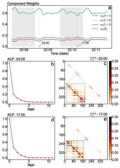
Figure 3: (a) Component weights for generating $\boldsymbol{C}_{t}$ for a batch of time series ($B=8$) from the $\mathtt{m4\_hourly}$ dataset obtained by the GPVar model. Parameters $w_{0},w_{1},w_{2}$ represent the component weights of the kernel matrices associated with lengthscales $l=1,2,3$, and $w_{3}$ is the component weight for the identity matrix. Shaded areas distinguish different days; (b) and (d): The autocorrelation function (ACF) indicated by the error correlation matrix $\boldsymbol{C}_{t}$ at 3:00 and 17:00. Given the rapid decay of the ACF, we only plot 12 lags to enhance visualization; (c) and (e): The corresponding covariance matrix of the associated target variables $\boldsymbol{\Sigma}_{t}^{\text{bat}}=(\boldsymbol{L}_{t}^{\text{bat}})(\boldsymbol{C}_{t}\otimes\mathbf{I}_{R})(\boldsymbol{L}_{t}^{\text{bat}})^{\top}+\operatorname{diag}(\boldsymbol{d}_{t}^{\text{bat}})$ at 3:00 and 17:00. A zoomed-in view of a $3B\times 3B$ region is illustrated in both plots, where the diagonal blocks represent $B\times B$ covariance matrices $\boldsymbol{\Sigma}_{t^{\prime}}$ of $\mathbf{z}_{t^{\prime}}$ over three consecutive time steps. While the off-diagonal blocks describe the covariance $\operatorname{Cov}(\mathbf{z}_{t-\Delta},\mathbf{z}_{t})$, $\forall\Delta\neq 0$. To enhance the clarity of the visualization, covariance values are clipped to the range of 0 and 0.3.

5.2 Model Interpretation

Our method is designed to capture error autocorrelation through the dynamic construction of a covariance matrix. This is achieved by combining kernel matrices with varying lengthscales in a dynamic weighted sum. The selection of the lengthscale plays a pivotal role in shaping the autocorrelation structure. A small lengthscale corresponds to short-range positive autocorrelation, whereas a large lengthscale can capture positive correlation over long lags.

In Fig. 3, we depict the generated component weights and the resulting autocorrelation function (the first row of the learned correlation matrix $\boldsymbol{C}_{t}$) for a batch of time series from the $\mathtt{m4\_hourly}$ dataset spanning a four-day duration. The covariance matrix of $\boldsymbol{z}_{t}^{\text{bat}}$ over a mini-batch is also provided using the generated correlation matrices and model outputs at two different times of the day. In particular, we observe that the component weights $w_{3}$, corresponding to the identity matrix, dominate throughout the entire observation period. This suggests that the error autocorrelation is generally mild over time. This behavior is also influenced by our parameterization of autocorrelation across the mini-batch. Recalling the Kronecker structure employed for parameterizing the covariance over the low-dimensional latent variables $\boldsymbol{r}_{t^{\prime}}$ in a mini-batch, it assumes that each rank shares the same autocorrelation structure. Given the Kronecker structure, the model is inclined to learn the mildest autocorrelation among the time series in a batch.

Moreover, we observe the adjustment of correlation strengths facilitated by the dynamic component weights. Specifically, as the weight assigned to the identity matrix ($w_{3}$) increases, the error process tends to show greater independence. On the contrary, when the weights assigned to the other kernel matrices ($w_{0}$, $w_{1}$, and $w_{2}$) are larger, the error process becomes more correlated, since the kernel matrices with different lengthscales are combined to formulate a specific autocorrelation structure. Fig. 3 (a) highlights noticeable daily patterns in autocorrelation, especially showcasing heightened correlation among errors around 17:00 each day. Figs. 3 (b, d) indicate that the autocorrelation is less pronounced at 3:00 in the morning compared to what is observed at 17:00. This highlights the important need for our method to adjust the covariance matrix as needed, so we can effectively model the autocorrelation over time. Figs. 3 (c, e) show the covariance matrix of the target variables within the autocorrelation horizon. The diagonal blocks represent the covariance $\boldsymbol{\Sigma}_{t^{\prime}}$ of time series variables $\mathbf{z}_{t^{\prime}}$ at each time step, which models the correlations between time series. The off-diagonal blocks depict the covariance $\operatorname{Cov}(\mathbf{z}_{t-\Delta},\mathbf{z}_{t})$, $\forall\Delta\neq 0$ within the autocorrelation horizon that can be captured by our approach. The zoomed-in view provides a $3B\times 3B$ region that illustrates the autocorrelation within two lags. We can observe that the autocorrelation is most pronounced at lag 1, which is consistent with the observation of Fig. 3 (a) that the component weight $w_{0}$ assigned to the base kernel matrix with lengthscale $l=1$ is more pronounced than $w_{1}$ and $w_{2}$.

5.3 Computation Cost

Our approach results in additional training costs primarily due to the larger covariance matrix size, $DB\times DB$, compared to the conventional $B\times B$ matrix when evaluating the log-likelihood of the multivariate Gaussian distribution. The training cost comparison, detailed in Table 7 in Appendix §C.4, illustrates the impact of our method on the training time. Notably, it extends the time required per epoch to train the model across all scenarios. However, it is worth noting that our method does not necessarily correlate with an increase in the number of epochs needed for convergence. As demonstrated in Table 7, our method exhibits the potential to accelerate convergence in certain cases, which can be attributed to the more flexible assumptions regarding the error process.

6 Conclusion

This paper presents a novel approach to addressing error autocorrelation in multivariate probabilistic time series forecasting. The method involves constructing a dynamic covariance matrix based on a small set of independent and identically distributed latent temporal processes within a mini-batch. These latent processes allow us to effectively model error autocorrelation and they can be seamlessly integrated into the base model, in which the contemporaneous covaraince is parameterized by a low-rank-plus-diagonal structure. Our method enables the modeling and prediction of a time-varying covariance matrix for the target time series variable. We implement and assess the proposed method using GPVar and Transformer on various public datasets, demonstrating its effectiveness in enhancing uncertainty quantification. The contribution of our method is two-fold. First, given the common assumption of Gaussian errors in probabilistic forecasting models, our approach can improve the training process for such models. Second, the learned autocorrelation can enhance multistep-ahead predictions by refining the distribution output at each forecasting step.

There are several avenues for future research. Firstly, the Kronecker structure $\boldsymbol{C}_{t}\otimes\mathbf{I}_{R}$ for the covariance matrix of the latent variable $\boldsymbol{r}_{t}^{\text{bat}}$ in a mini-batch may prove to be too restrictive for multivariate time series problems. This is because we assume that the rows (ie, latent temporal processes) in the matrix $\left[\mathbf{r}_{t},\ldots,\mathbf{r}_{t+D-1}\right]$ are identically distributed following $\mathcal{N}\left(\boldsymbol{0},\boldsymbol{C}_{t}\right)$. Exploring more flexible covariance structures, such as employing $R$ different $\boldsymbol{C}_{r,t}$ for each of the latent temporal processes, could be a promising avenue for further investigation. Secondly, the parameterization of $\boldsymbol{C}_{t}$ could be further explored. Instead of using SE kernels, one could parameterize $\boldsymbol{C}_{t}$ as fully-learnable positive definite symmetric Toeplitz matrices. For instance, an AR($p$) process has covariance with a Toeplitz structure, allowing the modeling of negative correlations. This alternative approach may offer more flexibility in capturing complex correlation patterns in multivariate time series data.

Impact Statements

This paper presents work whose goal is to advance the field of Machine Learning. There are many potential societal consequences of our work, none which we feel must be specifically highlighted here.

Appendix A Dataset Details

We performed experiments on a diverse set of real-world datasets obtained from GluonTS (Alexandrov et al., 2020). These datasets include:

• $\mathtt{m4\_hourly}$ (Makridakis et al., 2020): Hourly time series data from various domains, covering microeconomics, macroeconomics, finance, industry, demographics, and various other fields, is sourced from the M4-competition.

• $\mathtt{exchange\_rate}$ (Lai et al., 2018): Daily exchange rate information for eight different countries spanning the period from 1990 to 2016.

• $\mathtt{m1\_quarterly}$ (Makridakis et al., 1982): Quarterly time series data spanning seven different domains.

• $\mathtt{pems03}$ (Chen et al., 2001): Traffic flow records obtained from Caltrans District 3 and accessed through the Caltrans Performance Measurement System (PeMS). The records are aggregated at a 5-minute interval.

• $\mathtt{solar}$ (Lai et al., 2018): Hourly time series representing solar power production data in the state of Alabama for the year 2006.

• $\mathtt{traffic}$ (Caltrans, 2015): Hourly traffic occupancy rates recorded by sensors installed in the San Francisco freeway system between January 2008 and June 2008.

• $\mathtt{uber\_hourly}$ (Commission, 2015): Hourly time series of Uber pickups in New York City spanning from February to July 2015.

These datasets are widely employed for benchmarking time series forecasting models, following their default configurations in GluonTS, including granularity, prediction range ($Q$) and the number of rolling evaluations. We split each dataset sequentially into training, validation, and testing sets. The temporal length of the validation set matched that of the testing set. The length of the testing set was determined based on the prediction range and the number of rolling evaluations required. For instance, the testing horizon for the $\mathtt{traffic}$ dataset is computed as $24+7-1=30$ time steps. Consequently, the model will predict 24 steps ($Q$) in a rolling manner with 7 different consecutive prediction start timestamps. In our experiments, we align the conditioning range ($P$) with the prediction range ($Q$), maintaining consistency with the default setting in GluonTS. For simplicity, we set the autocorrelation horizon ($D$) to also match the prediction range ($Q$). Essentially, in this paper, we have $P=Q=D$. The statistics of all datasets are summarized in Table 2.

Table 2: Dataset summary.

Dataset	Granularity	# of time series	# of time steps	$Q$	Rolling evaluation
$\mathtt{m4\_hourly}$	hourly	414	1,008	48	1
$\mathtt{exchange\_rate}$	workday	8	6,101	30	5
$\mathtt{m1\_quarterly}$	quarterly	203	48	8	1
$\mathtt{pems03}$	5min	358	26,208	12	24
$\mathtt{solar}$	hourly	137	7,033	24	7
$\mathtt{traffic}$	hourly	963	4,025	24	7
$\mathtt{uber\_hourly}$	hourly	262	4,344	24	1

Appendix B Additional Metrics

B.1 Root Relative Mean Squared Error

We also compare to classical methods including ARIMA (Box et al., 2015) and ETS exponential smoothing (Hyndman et al., 2008) using root relative mean squared error (RRMSE):

$$\operatorname{RRMSE}=\frac{\sqrt{\sum_{t}\left(z_{i}-\hat{z}_{t}\right)^{2}}}{\sqrt{\sum_{t}\left(z_{i}-\bar{z}_{i}\right)^{2}}},$$ (18)

where $\hat{z}_{i}$ is the sample mean, $\bar{z}_{i}$ is the mean value of the testing dataset. 100 samples were drawn from the predicted distribution to evaluate the sample mean. In this experiment, we employed the $\mathtt{auto.arima}$ function from the $\mathtt{pmdarima}$ package (Smith et al., 2017) and the $\mathtt{ETSModel}$ function from the $\mathtt{statsmodels}$ package (Seabold & Perktold, 2010). The $\mathtt{auto.arima}$ function automatically determines the optimal order for an ARIMA model. For the ETS model, the configuration for different types of datasets is summarized in Table 3. The temporal length of the training data was set to be ten times that of the prediction range. Note that results for datasets with insufficient temporal length (e.g., $\mathtt{m1\_quarterly}$) are not provided. The comparison results are summarized in Table 4.

Table 3: ETS model configuration for datasets with different temporal granularity.

Model parameters	workday/daily	hourly	other
error	✓	✓	✓
trend	✓	✓	✓
damped_trend	✓	✓	✓
seasonal	✓	✓	$\times$
seasonal_periods	7	24	N/A

Table 4: RRMSE accuracy comparison (lower is better, better performance is in boldface). “w/o” implies models optimized with the conventional multivariate Gaussian likelihood loss, whereas “w/” implies models combined with our method. Results are based on averaging the scores from running each model three times.

	auto.arima	ets	GPVar		Transformer
			w/o	w/	w/o	w/
$\mathtt{m4\_hourly}$	0.6058	0.6321	0.4004	0.3803	0.4085	0.3699
$\mathtt{exchange\_rate}$	0.0199	0.0199	0.0584	0.0222	0.0724	0.0302
$\mathtt{pems03}$	0.3921	0.3819	0.3861	0.3051	0.2922	0.3016
$\mathtt{solar}$	0.9699	0.8239	0.7251	0.8098	0.9566	0.9254
$\mathtt{traffic}$	0.8591	N/A	0.6728	0.6347	0.7167	0.6814
$\mathtt{uber\_hourly}$	0.5952	0.7653	0.3335	0.2908	0.3075	0.2836

B.2 Quantile Loss

We present the quantile loss ($\rho$-risk) (Salinas et al., 2020) as additional metrics for further exploration of the probabilistic forecasting performance:

$$L_{\rho}\left(Z,\hat{Z}^{\rho}\right)=2(\hat{Z}^{\rho}-Z)\left((1-\rho)\mathrm{I}_{\hat{Z}^{\rho}>Z}-\rho\mathrm{I}_{\hat{Z}^{\rho}\leq Z}\right),$$ (19)

where $\mathrm{I}$ is a binary indicator function that equals 1 when the condition is met, $\hat{Z}^{\rho}$ represents the predicted $\rho$-quantile, and $Z$ represents the ground truth value. The quantile loss serves as a metric to assess the accuracy of a given quantile, denoted by $\rho$, from the predictive distribution. We summarize the quantile losses for the testing set across all time series segments by evaluating a normalized summation of these losses: $\left(\sum_{i}L_{\rho}\left(Z_{i},\hat{Z}_{i}^{\rho}\right)\right)/\left(\sum_{i}Z_{i}\right)$. In this paper, we evaluate the $0.5$-risk and the $0.9$-risk following Salinas et al. (2020). 100 samples were drawn from the predicted distribution to evaluate the quantile loss. The results are summarized in Table 5 and Table 6.

Table 5: $0.5$-risk accuracy comparison (lower is better, better performance is in boldface). “w/o” implies models optimized with the conventional multivariate Gaussian likelihood loss, whereas “w/” implies models combined with our method. Mean and standard deviation are obtained by running each model three times.

	GPVar		Transformer
	w/o	w/	w/o	w/
$\mathtt{m4\_hourly}$	0.1085$\pm$0.0003	0.1019$\pm$0.0005	0.1133$\pm$0.0003	0.0990$\pm$0.0004
$\mathtt{exchange\_rate}$	0.0084$\pm$0.0000	0.0048$\pm$0.0001	0.0151$\pm$0.0003	0.0055$\pm$0.0000
$\mathtt{m1\_quarterly}$	0.2160$\pm$0.0007	0.1965$\pm$0.0017	0.2429$\pm$0.0011	0.2222$\pm$0.0023
$\mathtt{pems03}$	0.0832$\pm$0.0001	0.0641$\pm$0.0001	0.0600$\pm$0.0000	0.0617$\pm$0.0000
$\mathtt{solar}$	0.4533$\pm$0.0010	0.3761$\pm$0.0007	0.4244$\pm$0.0001	0.4016$\pm$0.0009
$\mathtt{traffic}$	0.1276$\pm$0.0003	0.1256$\pm$0.0002	0.1560$\pm$0.0002	0.1299$\pm$0.0001
$\mathtt{uber\_hourly}$	0.1364$\pm$0.0006	0.1192$\pm$0.0004	0.1319$\pm$0.0002	0.1297$\pm$0.0004

Table 6: $0.9$-risk accuracy comparison (lower is better, better performance is in boldface). “w/o” implies models optimized with the conventional multivariate Gaussian likelihood loss, whereas “w/” implies models combined with our method. Mean and standard deviation are obtained by running each model three times.

	GPVar		Transformer
	w/o	w/	w/o	w/
$\mathtt{m4\_hourly}$	0.0586$\pm$0.0007	0.0584$\pm$0.0002	0.0645$\pm$0.0009	0.0506$\pm$0.0002
$\mathtt{exchange\_rate}$	0.0034$\pm$0.0000	0.0031$\pm$0.0000	0.0057$\pm$0.0001	0.0028$\pm$0.0000
$\mathtt{m1\_quarterly}$	0.3235$\pm$0.0032	0.2874$\pm$0.0041	0.3894$\pm$0.0024	0.3118$\pm$0.0043
$\mathtt{pems03}$	0.0495$\pm$0.0000	0.0303$\pm$0.0000	0.0289$\pm$0.0000	0.0299$\pm$0.0000
$\mathtt{solar}$	0.2140$\pm$0.0011	0.3015$\pm$0.0013	0.4564$\pm$0.0020	0.4033$\pm$0.0016
$\mathtt{traffic}$	0.1042$\pm$0.0002	0.0987$\pm$0.0002	0.1024$\pm$0.0004	0.1010$\pm$0.0001
$\mathtt{uber\_hourly}$	0.0710$\pm$0.0008	0.0609$\pm$0.0001	0.0654$\pm$0.0002	0.0621$\pm$0.0002

Appendix C Experiment Details

C.1 Model Architecture

In this study, we use GPVar (Salinas et al., 2019) and a decoder-only autoregressive Transformer model, specifically the GPT model (Radford et al., 2018), as our base probabilistic models. For the GPVar model, the network receives inputs at each time step $t$ consisting of the target variable from the previous time step $\mathbf{z}_{t-1}$, covariates $\mathbf{x}_{t}$ of the current time step, and the hidden state $\mathbf{h}_{t-1}$. The network output $\mathbf{h}_{t}$ is then used to compute the distribution parameters $\theta(\mathbf{h}_{t})=(\boldsymbol{\mu}_{t},\boldsymbol{L}_{t},\mathbf{d}_{t})$. During the training phase, the ground truth values of the target variable serve as inputs for both the conditioning range and the prediction range. No sampling is necessary for the prediction range. In the testing phase, a sample $\tilde{\mathbf{z}}\sim\mathcal{N}\left(\bar{\boldsymbol{\mu}}_{t},\bar{\boldsymbol{\Sigma}}_{t}\right)$ is drawn and utilized as input for the subsequent time step in the prediction range, resulting in the creation of a single sample trace. Repeating this prediction process generates multiple traces collectively representing the jointly predictive distribution. In our framework, the component weights $\mathbf{w}_{m,t}$ are derived from the same hidden state $\mathbf{h}_{t}$ used for projecting the $\theta_{t}$. For the Transformer model, we adapt the output to match the parameters of the predictive distribution, similar to the GPVar model. To maintain the autoregressive property, we apply a subsequent mask to the input sequence, ensuring that attention scores are computed exclusively based on the inputs preceding the current time step.

C.2 Covariates

The covariates in our models are known features for both past and future time steps. In cases of time-varying covariates, we use “hour of day” and “day of week” as covariates for datasets with hourly granularity, and use ”day of week” as the sole covariate for daily datasets. In cases of static covariates, we use the identifiers of the time series. These covariates are concatenated with the RNN or Transformer input at each time step following their encoding by the embedding layer. Additionally, we normalize the target values of the time series by scaling them with the mean and standard deviation specific to each time series, derived from the training dataset.

C.3 Hyperparameters

The batch size for all models is fixed at 32. The LSTM hyperparameters in GPVar are consistent with those outlined in (Salinas et al., 2019). This includes utilizing three layers of LSTM, each with 40 nodes, and setting the dropout rate to 0.1. For the distribution head, a single linear layer is employed to output the distribution parameters. A series of distinct linear layers and ELU layers are utilized for generating the component weights. To ensure parity in the number of parameters between Transformer and GPVar, we configure the Transformer with three stacked decoding layers. These layers have a hidden size of 42, $H=2$ attention heads, and a dropout rate of 0.1.

C.4 Training Details

Each model underwent training for a maximum of 100 epochs, employing a learning rate of 0.001 and the Adam optimizer. The training procedure incorporated an early stopping strategy with a patience of 10 epochs. Upon completion of training, the optimal model, as identified by the validation loss, was restored. The training cost per epoch and the number of epochs documented for terminating the training process are detailed in Table 7.

Table 7: Training cost comparison. “w/o” implies models optimized with the conventional multivariate Gaussian likelihood loss, whereas “w/” implies models combined with our method.

	GPVar				Transformer
	w/o		w/		w/o		w/
	sec./epoch	epochs	sec./epoch	epochs	sec./epoch	epochs	sec./epoch	epochs
$\mathtt{m4\_hourly}$	8	99	65	99	7	99	9	99
$\mathtt{exchange\_rate}$	5	44	27	52	5	33	6	86
$\mathtt{m1\_quarterly}$	6	10	10	10	7	52	8	11
$\mathtt{pems03}$	24	80	38	48	26	71	32	50
$\mathtt{solar}$	11	49	30	83	12	47	13	93
$\mathtt{traffic}$	23	43	53	60	22	74	26	92
$\mathtt{uber\_hourly}$	7	71	25	88	8	70	9	59

C.5 Hardware Environment

Our experiments were conducted under a computer environment with one Intel(R) Xeon(R) CPU E5-2698 v4 @ 2.20GHz and four NVIDIA Tesla V100 GPU.

References

- Alexandrov et al. (2020) Alexandrov, A., Benidis, K., Bohlke-Schneider, M., Flunkert, V., Gasthaus, J., Januschowski, T., Maddix, D. C., Rangapuram, S., Salinas, D., Schulz, J., et al. Gluonts: Probabilistic and neural time series modeling in python. The Journal of Machine Learning Research, 21(1):4629–4634, 2020.
- Ashok et al. (2023) Ashok, A., Marcotte, É., Zantedeschi, V., Chapados, N., and Drouin, A. Tactis-2: Better, faster, simpler attentional copulas for multivariate time series. arXiv preprint arXiv:2310.01327, 2023.
- Bai et al. (2020) Bai, L., Yao, L., Li, C., Wang, X., and Wang, C. Adaptive graph convolutional recurrent network for traffic forecasting. Advances in Neural Information Processing Systems, 33:17804–17815, 2020.
- Beitner (2020) Beitner, J. Pytorch forecasting. https://pytorch-forecasting.readthedocs.io, 2020.
- Benidis et al. (2022) Benidis, K., Rangapuram, S. S., Flunkert, V., Wang, Y., Maddix, D., Turkmen, C., Gasthaus, J., Bohlke-Schneider, M., Salinas, D., Stella, L., et al. Deep learning for time series forecasting: Tutorial and literature survey. ACM Computing Surveys, 55(6):1–36, 2022.
- Box et al. (2015) Box, G. E., Jenkins, G. M., Reinsel, G. C., and Ljung, G. M. Time series analysis: forecasting and control. John Wiley & Sons, 2015.
- Caltrans (2015) Caltrans. Caltrans performance measurement system. URL https://pems.dot.ca.gov/, 2015.
- Chen et al. (2001) Chen, C., Petty, K., Skabardonis, A., Varaiya, P., and Jia, Z. Freeway performance measurement system: mining loop detector data. Transportation Research Record, 1748(1):96–102, 2001.
- Choi et al. (2022) Choi, S., Saunier, N., Trepanier, M., and Sun, L. Spatiotemporal residual regularization with dynamic mixtures for traffic forecasting. arXiv preprint arXiv:2212.06653, 2022.
- Commission (2015) Commission, N. T. L. Uber tlc foil response, 2015.
- de Bézenac et al. (2020) de Bézenac, E., Rangapuram, S. S., Benidis, K., Bohlke-Schneider, M., Kurle, R., Stella, L., Hasson, H., Gallinari, P., and Januschowski, T. Normalizing kalman filters for multivariate time series analysis. Advances in Neural Information Processing Systems, 33:2995–3007, 2020.
- Drouin et al. (2022) Drouin, A., Marcotte, É., and Chapados, N. Tactis: Transformer-attentional copulas for time series. In International Conference on Machine Learning, pp. 5447–5493. PMLR, 2022.
- Gneiting & Raftery (2007) Gneiting, T. and Raftery, A. E. Strictly proper scoring rules, prediction, and estimation. Journal of the American statistical Association, 102(477):359–378, 2007.
- Hamilton (2020) Hamilton, J. D. Time Series Analysis. Princeton University Press, 2020.
- Hyndman et al. (2008) Hyndman, R., Koehler, A. B., Ord, J. K., and Snyder, R. D. Forecasting with exponential smoothing: the state space approach. Springer Science & Business Media, 2008.
- Hyndman & Athanasopoulos (2018) Hyndman, R. J. and Athanasopoulos, G. Forecasting: Principles and Practice. OTexts, 2018.
- Jia & Benson (2020) Jia, J. and Benson, A. R. Residual correlation in graph neural network regression. In Proceedings of the 26th ACM SIGKDD International Conference on Knowledge Discovery & Data Mining, pp. 588–598, 2020.
- Lai et al. (2018) Lai, G., Chang, W.-C., Yang, Y., and Liu, H. Modeling long-and short-term temporal patterns with deep neural networks. In The 41st international ACM SIGIR conference on research & development in information retrieval, pp. 95–104, 2018.
- Makridakis et al. (1982) Makridakis, S., Andersen, A., Carbone, R., Fildes, R., Hibon, M., Lewandowski, R., Newton, J., Parzen, E., and Winkler, R. The accuracy of extrapolation (time series) methods: Results of a forecasting competition. Journal of forecasting, 1(2):111–153, 1982.
- Makridakis et al. (2020) Makridakis, S., Spiliotis, E., and Assimakopoulos, V. The m4 competition: 100,000 time series and 61 forecasting methods. International Journal of Forecasting, 36(1):54–74, 2020.
- Prado et al. (2021) Prado, R., Ferreira, M. A., and West, M. Time Series: Modeling, Computation, and Inference. CRC Press, 2021.
- Radford et al. (2018) Radford, A., Narasimhan, K., Salimans, T., Sutskever, I., et al. Improving language understanding by generative pre-training. 2018.
- Rangapuram et al. (2018) Rangapuram, S. S., Seeger, M. W., Gasthaus, J., Stella, L., Wang, Y., and Januschowski, T. Deep state space models for time series forecasting. Advances in neural information processing systems, 31, 2018.
- Rasul et al. (2020) Rasul, K., Sheikh, A.-S., Schuster, I., Bergmann, U., and Vollgraf, R. Multivariate probabilistic time series forecasting via conditioned normalizing flows. arXiv preprint arXiv:2002.06103, 2020.
- Rasul et al. (2021) Rasul, K., Seward, C., Schuster, I., and Vollgraf, R. Autoregressive denoising diffusion models for multivariate probabilistic time series forecasting. In International Conference on Machine Learning, pp. 8857–8868. PMLR, 2021.
- Saha et al. (2023) Saha, A., Basu, S., and Datta, A. Random forests for spatially dependent data. Journal of the American Statistical Association, 118(541):665–683, 2023.
- Salinas et al. (2019) Salinas, D., Bohlke-Schneider, M., Callot, L., Medico, R., and Gasthaus, J. High-dimensional multivariate forecasting with low-rank gaussian copula processes. Advances in neural information processing systems, 32, 2019.
- Salinas et al. (2020) Salinas, D., Flunkert, V., Gasthaus, J., and Januschowski, T. Deepar: Probabilistic forecasting with autoregressive recurrent networks. International Journal of Forecasting, 36(3):1181–1191, 2020.
- Seabold & Perktold (2010) Seabold, S. and Perktold, J. Statsmodels: Econometric and statistical modeling with python. In Proceedings of the 9th Python in Science Conference, volume 57, pp. 10–25080. Austin, TX, 2010.
- Shih et al. (2019) Shih, S.-Y., Sun, F.-K., and Lee, H.-y. Temporal pattern attention for multivariate time series forecasting. Machine Learning, 108:1421–1441, 2019.
- Smith et al. (2017) Smith, T. G. et al. pmdarima: Arima estimators for Python, 2017. URL http://www.alkaline-ml.com/pmdarima. [Online; accessed ¡today¿].
- Song et al. (2021) Song, D., Chen, H., Jiang, G., and Qin, Y. Dual stage attention based recurrent neural network for time series prediction, February 23 2021. US Patent 10,929,674.
- Sun et al. (2021) Sun, F.-K., Lang, C., and Boning, D. Adjusting for autocorrelated errors in neural networks for time series. Advances in Neural Information Processing Systems, 34:29806–29819, 2021.
- Tang & Matteson (2021) Tang, B. and Matteson, D. S. Probabilistic transformer for time series analysis. Advances in Neural Information Processing Systems, 34:23592–23608, 2021.
- Wang et al. (2019) Wang, Y., Smola, A., Maddix, D., Gasthaus, J., Foster, D., and Januschowski, T. Deep factors for forecasting. In International conference on machine learning, pp. 6607–6617. PMLR, 2019.
- Wen et al. (2017) Wen, R., Torkkola, K., Narayanaswamy, B., and Madeka, D. A multi-horizon quantile recurrent forecaster. arXiv preprint arXiv:1711.11053, 2017.
- Zhan & Datta (2023) Zhan, W. and Datta, A. Neural networks for geospatial data. arXiv preprint arXiv:2304.09157, 2023.
- Zheng et al. (2023a) Zheng, V. Z., Choi, S., and Sun, L. Better batch for deep probabilistic time series forecasting. arXiv preprint arXiv:2305.17028, 2023a.
- Zheng et al. (2023b) Zheng, V. Z., Choi, S., and Sun, L. Enhancing deep traffic forecasting models with dynamic regression. arXiv preprint arXiv:2301.06650, 2023b.