Hitting probability for Reflected Brownian Motion at Small Target

Abstract.

We derive the asymptotic behavior of hitting probability at small target of size $O(\epsilon)$ for reflected Brownian motion in domains with suitable smooth boundary conditions, where the boundary of domain contains both reflecting part, absorbing part and target. In this case the domain could be localized near the target and explicit computations are possible. The asymptotic behavior is only related to $\epsilon$ up to some multiplicative constants that depends on the domain and boundary conditions.

1. Introduction

Reflected Brownian motions, or more generally reflected Wiener processes, can roughly be thought as a Brownian motion that is “reflected” when it hits some targets. Although it has simple intuitive description, it is extremely hard to construct Reflected Brownian motions in domains in $\mathbb{R}^{n}$ for $n\geq 2$ [1, 2]. Despite of this difficulty, reflected Brownian motion has became a great area of research in both pure mathematics and applied mathematics [1, 3, 4]. In particular, its hitting behavior at small targets has grasped the interests of more and more researchers [5, 6]. Despite there has been some works done in asymptotic hitting behaviors of Brownian motions at small targets [7, 8], the asymptotic hitting behaviors of reflected Brownian Motions at small targets is poorly understood.

In this paper we will mainly be focused on asymptotic hitting probability for reflected Brownian motion at small targets. The current state of art in this area is preforming explicit computations using connections between reflected Brownian motion and partial differentiate equations, which was done by Denis S. Grebenkov and Adrien Chaigneau in certain domains [4]. However, this approach is limited to huge amount of computations and could only be done in a few domains where solutions to Dirichlet problem behaves nicely. Instead, in this paper we observed that the reflected Brownian motion behaves very well in a large class of domains which we defined to be “Smooth Uniform Lipchitz Domains” (see Definition 2.4), and in this class of domains the asymptotic behavior hitting probability is comparable to a fundamental solution of Laplacian. The intuition is when the reflect Brownian particle is near the target, the probability that it hits non-targeted boundary is very small and thus irrelevant to the universal shape of the domain. When target is very small, the local geometry of SULD domain near the target is nearly half space, so the asymptotic hitting probability should agree to the case of a half ball with target at the bottom planar surface, and computation could be done easily in this case.

Complex analysis, especially conformal maps and harmonic measures, has played a crucial role in studies of planar Brownian motions [9, 10]. We will also use methods from complex analysis to prove a more accurate result (see Theorem 3.4). Regrettably, this accurate result haven’t be generalized to higher dimensions as the method of complex analysis ceases to work.

Although this paper successfully computed the asymptotic behavior of hitting probability in a large class of domains, the asymptotic mean hitting time still remains open except for some elongated domains [6]. Besides, the asymptotic hitting probability for domains with rough boundaries (e.g. fractal domains) still remains open. The methods in this paper all cease to work for these kind of domains and even some basic properties of reflected Brownian motion hasn’t been well-studied for these domains yet.

In this paper, we will construct reflected Brownian motion in chapter 2, and show any analytic simply connected domain in $\mathbb{C}$ is SULD. Some technique proofs will be included in chapter 7 appendix. In chapter 3 we define the target, absorbing boundaries and state our main results (Theorem 3.3 and Theorem 3.4). In chapter 4 we cite some standard definitions and results in complex analysis. We will prove Theorem 3.3 and Theorem 3.4 using complex analysis tools in $\mathbb{C}$ in chapter 5 and prove Theorem 3.3 in higher dimension in chapter 6.

2. Domains and Construction of Reflected Brownian Motion

In this section we construct the reflected Brownian motions (RBM) in certain domains.

2.1. Construction of RBM on General (SULD) Domains

In this subsection we discuss how to define RBM on any connected domains in $\mathbb{R}^{n}$ $(n\geq 2)$ with suitable smooth and analytical conditions.

Definition 2.1.

Let $\Omega$ be a connected open set of $\mathbb{R}^{n}$. We say $\Omega$ is a smooth domain if at each point $x\in\partial\Omega$ there is an open ball $B_{x}$ centered at $x$ and a smooth bijection $\Phi_{x}:B_{x}\to D\subset\mathbb{R}^{n}$ with smooth inverse such that $\Phi_{x}(B_{x}\cap\Omega)\subset\mathbb{R}_{+}^{n}:=\{(x_{1},...,x_{n}):x_{1}>0\}$ and $\Phi_{x}(B_{x}\cap\partial\Omega)\subset\partial\mathbb{R}_{+}^{n}$. We call $\Phi_{x}$ be the coordinate mapping associated with $B_{x}$.

There are many equivalent ways to construct RBM, in here we follow the construction by [2]. Constructions in more general domain could be done, for example, in [11] using Dirichlet form. We define the RBM by explicit construction of solution to stochastic differential equation which generate RBM in an intuitive sense. Let $\mathbb{H}_{n}:=\mathbb{R}^{n}_{+}$ be the upper half space in $\mathbb{R}^{n}$ and $W_{t}$ be a $n$-dimensional unrestricted standard Brownian motion. Consider the stochastic differential equation in $(X_{t}^{x},\xi_{t}^{x})$:

(1) $$dX_{t}^{x}=\mathrm{d}W_{t}+\mathbf{1}_{\partial\mathbb{H}_{n}}(X_{t}^{x})\gamma(X_{t}^{x})\mathrm{d}\xi_{t}^{x}$$

with $X_{0}^{x}=x$ and $\xi_{0}^{x}=0$, and $\gamma$ is a constant vector valued function with $\gamma\equiv(1,0,...,0)$. $(X_{t}^{x},\xi_{t}^{x})$ is adapted to the $\sigma$-algebra that with probability $1$, $\xi_{t}^{x}$ is non-decreasing in $t$ and increases only at set $\Delta:=\{t:X^{x}_{t}\in\partial\mathbb{H}_{n}\}$ and $\Delta$ is a Lebesgue null set. Now we use explicit construction to proof the following proposition

Proposition 2.2.

Under the condition above, the stochastic differential equation (1) has a unique solution pair $(X_{t}^{x},\xi_{t}^{x})$ in the sense that any other pair satisfies (1) and $\Delta$ be a Lebesgue null set is equal to this pair with probability 1. We define the reflected Brownian motion in $\mathbb{R}^{n}_{+}$ to be the process $X^{x}_{t}$.[2]

Proof.

We only proof its existence here. For uniqueness see [2]. Define a transformation $\Gamma:C\left(\mathbb{R}^{n}\right)\to C\left(\mathbb{R}_{+}^{n}\right)$ (the same symbol $\Gamma$ may be used when the parameter set is $[0,T])$ as follows: for $\zeta=\left(\zeta_{1},\zeta_{2},...,\zeta_{n}\right)\in C\left(\mathbb{R}_{n}\right),\eta=\Gamma(\zeta)$ is defined by $\eta=\left(\eta_{1},\eta_{2},...,\eta_{n}\right)$, where $\eta_{i}=\zeta_{i}$ for $i=2,3,\cdots,n$, and $\eta_{1}(t)=\zeta_{1}(t)-\displaystyle\left(\left(\inf_{0\leq s\leq t}\zeta_{1}(s)\right)\wedge 0\right)$. Write $\Gamma_{t}(\zeta)$ for $(\Gamma(\zeta))(t)$. Now define the transformation $\xi:C\left(\mathbb{R}^{d}\right)\to C(\mathbb{R})$ by $\Gamma(\zeta)-\zeta=(\xi(\zeta),0,\cdots,0)$ and write $\xi_{t}(\zeta)$ for $(\xi(\zeta))(t)$. Then follow the proof of proposition 1 of [2] we have that, if $Y_{t}^{x}$ is the standard Brownian motion in $\mathbb{R}^{n}$, then $X_{t}^{x}=\Gamma\circ Y_{t}^{x}$ and $\xi_{t}^{x}=\xi\circ Y_{t}^{x}$ solves (1) and $X^{x}_{t}$ and $\xi^{x}_{t}$ satisfy the conditions imposed in connection with (1) . The pair $(X_{t}^{x},\xi_{t}^{x})$ is uniquely determined by (1) and the associated conditions, i.e., any other pair satisfying (1) and the associated conditions is equal to $(X_{t}^{x},\xi_{t}^{x})$ with probability one. ∎

We introduce an equivalent formulation of RBM in $\mathbb{H}_{n}$.

Proposition 2.3.

Let $X^{x}_{t}$ be defined in 2.2. Let $Y^{x}_{t}=(Y^{x}_{1}(t),Y^{x}_{2}(t),...,Y^{x}_{n}(t))$ be the standard Brownian motion in $R^{n}$ such that $Y^{x}_{0}=x=(x_{1},x_{2},...,x_{n})\in\mathbb{H}_{n}$ and each $Y_{k}^{x}(t)$ is the independent one dimensional Brownian motion. Define the process

$$Y^{x}_{t}=(|Y^{x}_{1}(t)|,Y^{x}_{2}(t),...,Y^{x}_{n}(t))$$

and the associated local time process

$$L_{t}^{x}=\frac{1}{2}\int_{0}^{t}\delta\left(Y^{x}_{1}(s)\right)ds.$$

Then $(Y^{x}_{t},L^{x}_{t})$ is equal to $(X_{t}^{x},\xi_{t}^{x})$ constructed in Proposition 2.2 with probability 1.

Proof.

By Itô’s formula we have

$$|Y_{1}^{x}(t)|=\int_{0}^{t}\operatorname{sign}\left(Y^{x}_{1}(s)\right)dY^{x}_{1}(s)+\frac{1}{2}\int_{0}^{t}\delta\left(Y^{x}_{1}(s)\right)ds=Y^{x}_{1}(t)+\frac{1}{2}\int_{0}^{t}\delta\left(Y^{x}_{1}(s)\right)ds$$

thus $(Y^{x}_{t},L^{x}_{t})$ satisfies (1). As Brownian motion spend almost zero time on any point set we see that $\Delta=\{t:Y^{x}_{1}(t)=0\}$ is a Lebesgue null set. So by Proposition 2.2 we see that $(Y^{x}_{t},L^{x}_{t})$ is equal to $(X_{t}^{x},\xi_{t}^{x})$ with probability 1. ∎

Now for a general domain $\Omega$ with smooth boundary and satisfies some conditions, we may construct the RBM in the following way. We firstly give the definition of a “Smooth Uniform Lipchitz domain” (SULD) in any dimension.

Definition 2.4.

We say $\Omega\subset\mathbb{R}^{n}$ is a SULD if it satisfies the following conditions:

1. $\Omega$ is a connected smooth domain;

2. $\Omega$ can be covered by $\mathscr{U}=\left\{U^{0},U^{1},...\right\}$ which is a countable family of open cover of $\overline{\Omega}$ where $U^{0}\subseteq\Omega$ is equipped with the original Euclidean coordinate of $\mathbb{R}^{n}$ which defines $\Omega$ and $\{U^{i}:i\geq 1\}\subset\{B_{x}:x\in\partial\Omega\}$ where $B_{x}$ are defined in Definition 2.1;

3. Let $\Phi_{k}$ be the coordinate mapping associated with $U^{k}$ defined in Definition 2.1. We require $\Phi_{k}$ maps normal on $U^{k}\cap\partial\Omega$ to a vector pointing towards $(1,0,0,...,0)$, which is equivalent to $\nabla\Phi^{i}_{k}\cdot\gamma=\delta_{1i}|\nabla\Phi^{i}_{k}|$.

4. We will suppose all $(\Phi_{k}:k\geq 1)$ satisfies uniform Lipchitz condition in the sense that there is an universal constant $\mathscr{C}$ that

   $$\frac{|x-y|}{\mathscr{C}}\leq|\Phi_{k}(x)-\Phi_{k}(y)|\leq\mathscr{C}|x-y|$$

   for all $k\geq 1$ and $x,y\in U^{k}$. We will also require the following conditions: There exists constants $\mathscr{C}_{1},\mathscr{C}_{2},\mathscr{C}_{3}$ such that

   $$\max\left\{\left\lVert\frac{\partial\Phi^{i}_{k}}{\partial x_{j}}\right\rVert_{\infty},\lVert\Delta\Phi_{k}^{i}\rVert_{\infty}\right\}\leq\mathscr{C}_{1},\quad\max\left\{\mathrm{Lip}\left(\frac{\partial\Phi^{i}_{k}}{\partial x_{j}}\right),\mathrm{Lip}\left(\Delta\Phi_{k}^{i}\right)\right\}\leq\mathscr{C}_{2}.$$

   for all $k$, $j$ where $\mathrm{Lip}(f)$ denotes the Lipchitz constant of $f$. Finally if we let $J^{k}$ be the Jacobian of $\Phi_{k}$ then $A_{k}=J_{k}J_{k}^{T}$ satisfies

   $$\mathscr{C}^{-1}_{3}|x|^{2}\leq x^{T}A_{k}x\leq\mathscr{C}_{3}|x|^{2}$$

   for all $k$, $j$ and $x\in\mathbb{R}^{n}$.

SULD represents a large class of domains as we shall see analytic domains in $\mathbb{C}$ are generally SULD (Proposition 2.9). Now we can construct RBM in SULD following [2].

Proposition 2.5.

Let $\Omega$ be a SULD, and $\gamma(x)$ be a vector field varies smoothly on the boundary and uniformly bounded away from tangent space of the boundary at $x$. then the stochastic differential equation

(2) $$dX_{t}^{x}=\mathrm{d}W_{t}+\mathbf{1}_{\partial\Omega}(X_{t}^{x})\gamma(X_{t}^{x})\mathrm{d}\xi_{t}^{x}$$

has a unique solution pair $(X_{t}^{x},\xi_{t}^{x})$ in the sense that any other pair is equal to this pair with probability 1. In particular when $\gamma$ is the unit normal vector at each $x$, we define the reflected Brownian motion in $\Omega$ to be the corresponding solution process process $X^{x}_{t}$.[2]

Proof.

(Existence part) We let $x\in\Omega$ and there exists an non negative integer $k(x)$ such that positive number $r=r(x)$ such that $B_{x}(r)\subset U^{k(x)}$. We use the coordinate patch of $U^{k(x)}$. We will construct the process in $B_{x}(r)$ until the time $S_{1}$ that it leaves $B_{x}(r)$. Then we will keep constructing until the last time $S_{2}$ before the process leaves the associated ball around ${X^{x}_{S_{1}}}$ and so on. For the first step we have the following cases:

1. If $k(x)=0$ only then the process is just the normal Brownian motion as boundary is not involved;

2. If we can choose $k(x)>0$ then the coordinate mapping $\Phi_{k}$ associated with $U^{k(x)}$ changes the problem to a problem in the upper half space with normal reflection on boundary. The new process $\Phi_{k}(X_{t})$ satisfies a new stochastic differential equation by itô’s formula: Write $\Phi_{k}=f=(f^{1},...,f^{n})$, then

   $$\mathrm{d}f^{i}(X_{t})=\left(\sum^{n}_{k=1}\frac{\partial f^{i}}{\partial x_{k}}\mathrm{d}W^{k}_{t}\right)+\frac{1}{2}\Delta f^{i}\mathrm{d}t+\mathbf{1}_{\partial\Phi_{k}(U_{k})\cap\overline{\mathbb{H}}}(f(X_{t}))\delta_{i1}|\nabla f^{1}|\mathrm{d}\xi_{t}$$

   where $(W^{1}_{t},...,W^{n}_{t})$ is the standard $n$ dimensional Brownian motion. By our assumption on the domain, this stochastic differential equation has a unique solution by [2] (proposition 1), with local time changed to

   $$\Xi_{t}=\int^{t}_{0}|\nabla f^{1}(B_{t})|\mathrm{d}\xi_{t}$$

3. This problem was solved above and we obtain a process in the upper half space with normal reflection. Then $\Phi^{-1}_{k}$ maps the process in upper half space back to $U^{k(x)}$ which gives us $X_{t}^{x},0\leq t\leq S_{1}$. For this process $(1)$ will hold, with $\xi_{t}^{x}$ being identical to the local time on the boundary for the process in upper half space. Then we just repeat this and gives us the desired process.

∎

However, non-uniqueness choices of $k(x)$ result in the same process. We will have to additionally show the consistency of our definition which is missed in [2].

Proposition 2.6.

Suppose $\mathscr{V}=\left\{V^{0},V^{1},...\right\}$ is another cover of $\Omega$ defined in 2.4 and $(\Psi_{k})_{k\geq 1}$ be another collection of associated maps. Suppose for some $k$ and $m$ that $V_{m}\cap U_{k}$ is non-empty. Then the transition map

$$\Phi_{k}\circ(\Psi_{m})^{-1}:\Psi_{m}(V_{m}\cap U_{k})\to\Phi_{k}(V_{m}\cap U_{k})$$

maps process $\Psi_{m}(X^{x}_{t})$ to the process $\Phi_{k}(X^{x}_{t})$.

Proof.

See Appendix, 7.1. ∎

We give another equivalent construction of RBM in analytic simply connected domains in $\mathbb{C}$ as a special case in order to apply tools in complex analysis to proof a stronger result.

2.2. Construction of RBM on Analytic Simply Connected Domains in $\mathbb{C}$

Definition 2.7.

Let $\Omega\subsetneq\mathbb{C}$ be a domain in the sense that it is open and connected. Let $\partial\Omega:=\bar{\Omega}\setminus\mathring{\Omega}$. We say $\Omega$ is analytic if there is an univalent function $f$ analytic near $\partial\mathbb{D}$ such that $\partial\Omega$ is the image of $\partial\mathbb{D}$ under $f$. We say $\Omega$ is analytic simply connected domain if it is additionally simply connected.

One equivalent construction of the RBM on analytic domain is using conformal mapping. We define RBM in upper half plane $\mathbb{H}$ then define the RBM in general analytic simply connected domain $\Omega$ by conformal maps, where Riemann mapping theorem ensure there is an conformal map between $\mathbb{H}$ and $\Omega$.

Definition 2.8.

Let $(X_{t},Y_{t})$ be the standard Brownian motion in $\mathbb{R}^{2}$ where $X_{t},Y_{t}$ are independent standard Brownian motion in $\mathbb{R}$. Define another stochastic process $B_{t}=(X_{t},|Y_{t}|)$ as the (complex) reflected Brownian motion in $\mathbb{H}$. Identify $\mathbb{C}$ with $\mathbb{R}^{2}$ our reflected Brownian motion in $\mathbb{H}$ is $B_{t}=X_{t}+i|Y_{t}|$. We write $B^{z}_{t}$ to denote the reflected Brownian motion starts at $z$. We also note the process $X_{t}+iY_{t}$ is referred to the complex Brownian motion by [9].

By Proposition 2.3 we see the stochastic process $B_{t}$ is equal to RBM in $\mathbb{H}$ constructed in proof of Proposition 2.2 with probability 1. We now construct RBM in unit disk $\mathbb{D}:=\{z\in\mathbb{C}:|z|<1\}$.

Proposition 2.9.

$\mathbb{D}$ is a SULD. More over, any domain $\Omega$ defined in Definition 2.7 is a SULD.

Proof.

See Appendix, 7.2. ∎

By the above proof and Proposition 2.5 we can construct the RBM in $\mathbb{D}$. Alternatively we have another equivalent construction of RBM in $\mathbb{D}$. We firstly prove a powerful characterisation of conformal invariance of RBM in $\mathbb{H}$.

Proposition 2.10.

Suppose $\Omega$ and $\Omega^{\prime}$ are two simply connected open subset of $\mathbb{H}$ and $B^{z_{0}}_{t}$ is the RBM in $\mathbb{H}$ where $z_{0}\in\Omega$ with the associated local time process $\xi^{z_{0}}_{t}$. Let $f$ be a conformal automorphism of $\mathbb{H}$. Let $\tau_{\Omega}=\inf\{t\geq 0:B^{z_{0}}_{t}\in\partial\Omega\}$. Then with probability one, $(f(B^{z_{0}}_{t}),t\in[0,\tau))$ is equal to the time-changed RBM in $\mathbb{H}$.

Proof.

See Appendix, 7.4. ∎

By examine above proof and notice that any conformal map $f=u+iv$ from $\Omega$ to $\mathbb{H}$ that can be extended conformally between a neighborhood of $\Omega$ and $\mathbb{H}$ with finite number of singularities (as we may delete them as the probability that the complex Brownian motion hit them is 0) on $\partial\Omega$, we have a stronger proposition:

Proposition 2.11.

Let $f$ be a conformal map between $\Omega$ and $\mathbb{H}$. If $f$ can be extended conformally between a neighborhood $\Omega^{\prime}$ of $\Omega$ and $\mathbb{H}^{\prime}$ of $\mathbb{H}$ with finite number of singularities on $\partial\Omega$, then $f$ maps the complex RBM in $\Omega$ to a time-changed complex RBM in $\mathbb{H}$.

Proposition 2.12.

Let $B^{z}_{t}$ be defined in Definition 2.8. Let $\displaystyle{f(z)=i\frac{z-i}{z+i}}$. Then the process $f(B^{z}_{t})$ is the RBM started at $f(z)$ which is equivalent to complex RBM in $\mathbb{D}$ constructed by Proposition 2.5 after a suitable time change, which is denoted by $X^{f(z)}_{t}$.

Proof.

We notice that the point $\infty$ is mapped to $i$ by $f$, which could be removed from consideration as $\{i\}$ is a null set. We note that by above proposition $(f^{j})^{-1}\circ f$ is an automorphism of $\mathbb{H}$ and thus it maps $B^{z}_{t}$ to another time-changed complex RBM in $\mathbb{H}$. It follows that $f(z)$ is the time changed complex RBM in $\mathbb{D}$. ∎

By above arguments we can now give an equivalent definition of the complex RBM via conformal mapping:

Definition 2.13.

Suppose $B_{t}$ is the complex RBM in $\mathbb{D}$ and let $\Omega$ be an analytic simply connected domain. Let $g$ be the associated conformal map from $\Omega$ to $\mathbb{D}$ above. Then we define the process $\tilde{B_{t}}=g^{-1}(B_{t})$ to be the reflected Brownian motion in $\Omega$.

Proof.

By lemma 7.3 we see that $f$ could be extended so $f\circ(f^{i})^{-1}$ could be the associated maps (properties could be checked by procedure similarly to proof of proposition 2.9 and by open mapping theorem each open cover of $\mathbb{D}$ is mapped to open cover of $\Omega$ by $f$. ∎

We would like to finish this section by the following key proposition, which is a generalization of proposition 2.11. Its proof is also similar to the proof we did above.

Proposition 2.14.

Let $\Omega_{1}$ and $\Omega_{2}$ be two analytic simply connected domain. By Riemann mapping theorem there is a conformal map $f$ between $\Omega_{1}$ and $\Omega_{2}$ which could also be extended to a conformal map between open neighborhood of $\overline{\Omega_{1}}$ and $\overline{\Omega_{2}}$. Let $B_{t}$ be the complex RBM in $\Omega_{1}$, then $f(B_{t})$ is the time-changed complex RBM in $\Omega_{2}$, starts at $f(z_{0})$.

3. Main Result

In this section we define the hitting target, absorbing boundary and reflecting boundaries. We will also states our main result.

3.1. Description of Hitting Target

Definition 3.1.

(Absorbing Boundary, Target and Reflecting Boundary) Let $\Omega$ be a SULD in $\mathcal{S}=\mathbb{R}^{n}$ or $\mathcal{S}=\mathbb{C}$. Let $P$ be a point on $\partial\Omega$. Let $R>0$ be a fixed constant that $\left(\mathcal{S}\setminus\overline{B_{R}(P)}\right)\cap\partial\Omega$ is non-empty, which will be denoted by $\mathrm{abs}$.

Let $\epsilon>0$ be a very small constant ($\epsilon\ll R$) and then our target (which is also absorbing) is $B_{\epsilon}(P)\cap\partial\Omega$, which will be denoted by $\mathrm{tg}$.

Let our reflecting boundary be $\partial\Omega\setminus(\mathrm{abs}\cup\mathrm{tg})$ which will be denoted by $\mathrm{ref}$.

See Figure 1 for an example.

Throughout the paper we assume there is a path inside $\Omega$ that connects a point in $\mathrm{tg}$ and $\mathrm{abs}$.

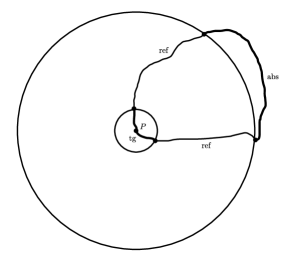
Figure 1. Absorbing Boundary, Reflecting Boundary and Target

We now give definition of the absorbing boundaries.

Definition 3.2.

Let $B^{x_{0}}_{t}$ be the reflected Brownian Motion in $\Omega$. Let $\tau=\inf\{t\geq 0:B^{x_{0}}_{t}\in\mathrm{abs}\cup\mathrm{tg}\}$ be the stopping time that RBM hits absorbing boundaries. We consider the stopped process $B^{x_{0}}_{\tau\wedge t}$ to be the RBM associated to the absorbing boundaries. In the later texts, without specification, $B^{x_{0}}_{t}$ denotes $B^{x_{0}}_{\tau\wedge t}$.

3.2. Main Result

The following theorem is our main result:

Theorem 3.3.

Let $\Omega$ be a SULD in $\mathbb{R}^{n}$ (identify $\mathbb{C}$ as $\mathbb{R}^{2}$) and $P$ be a point on $\partial\Omega$, with target, reflecting boundary and absorbing boundary defined above. Let $(B^{x_{0}}_{t},t>0)$ be the reflected Brownian Motion starting at $x_{0}\in\Omega$, and $\tau=\inf\{t\geq 0:B^{x_{0}}_{t}\in\mathrm{abs}\}$. Define

$$G_{n,y}(x)=\begin{cases}-\frac{1}{(n-2)\omega_{n-1}}|x-y|^{2-n}&\text{ if }n\in\mathbb{N}\backslash\{2\}\\ \frac{1}{\omega_{1}}\log|x-y|&\text{ if }n=2\end{cases}$$

be the generalized Newtonian potential, then there exists non-zero, positive constants $C_{1},C_{2}$ determined by $\Omega$ and $z_{0}$ such that

$$\frac{C_{1}}{G_{n,0}(\bm{\epsilon})}\leq\mathbb{P}(B^{x_{0}}_{\tau}\in\mathrm{tg})\leq\frac{C_{2}}{G_{n,0}(\bm{\epsilon})}$$

where $\bm{\epsilon}=(\epsilon,0,0...,0)\in\mathbb{R}^{n}$, for all $\epsilon$ small enough.

We have a stronger result, which confirm the asymptotic behavior of $\mathbb{P}(B^{z_{0}}_{\tau}\in\mathrm{tg})$ for certain domain.

Theorem 3.4.

Let $\Omega$ be an analytic simply connected domain in $\mathbb{C}$. If in addition there is only one component of absorbing boundary, then there exists a constant $C(\Omega,z_{0})$ that depends on $\Omega$ and starting point $z_{0}$ such that

$$\lim_{\epsilon\downarrow 0}\mathbb{P}(B^{z_{0}}_{\tau}\in\mathrm{tg})\log\epsilon=C(\Omega,z_{0}).$$

4. Standard Definitions and Standard Theorems

In this section we give some definitions to avoid confusions. Also we quote some useful standard theorems and lemmas.

Definition 4.1.

A conformal map between two domain is a holomorphic bijection between these two domains. [12] pp.206

Theorem 4.2.

(Riemann Mapping Theorem) Let $\Omega$ be a simply connected domain and $\Omega\neq\mathbb{C}$, then there exists a conformal map between $\Omega$ and $\mathbb{D}$. [12] Chapter 8, Theorem 3.1

We also note a uniqueness result.

Theorem 4.3.

Let $f$ be a conformal bijection between $\mathbb{D}$ and $\Omega$ where $\Omega$ is an analytic simply connected domain. Then by lemma 7.3 $f$ may be extended to a conformal bijection $g$. If in addition we fix two point on $\partial\Omega$ together with their derivatives, then such $f$ is unique.

We also have the following very useful Christoffel-Schwarz formula which maps $\mathbb{H}$ onto polygons.

Theorem 4.4.

Assume $\displaystyle\sum^{n-1}_{k=1}\beta_{k}<2$. Let $\mathfrak{p}$ be a polygonal region in the complex plane with vertexs $a_{1}$, $a_{2}$, …, $a_{n}$ where the angle at vertex $a_{k}$ for $k<n$ is $(1-\beta_{k})\pi$ and the angle at vertex $a_{n}$ is $(1-\beta_{n})\pi$ where

$$\beta_{n}=2-\sum_{k=1}^{n-1}\beta_{k}.$$

Let $F$ be a conformal map from the upper half-plane to $\mathfrak{p}$ such that the points $A_{1},\ldots,A_{n-1},\infty=A_{n}$ on $\mathbb{R}$ are sent to the vertices of $\mathfrak{p}$ where $A_{k}$ is sent to $a_{k}$. Then there exist unique constants $C_{1}$ and $C_{2}$ such that

$$F(z)=C_{1}\int_{0}^{z}\frac{d\zeta}{\left(\zeta-A_{1}\right)^{\beta_{1}}\cdots\left(\zeta-A_{n-1}\right)^{\beta_{n-1}}}+C_{2}.$$

where $(\zeta-A_{k})^{\beta_{k}}$ is defined by cutting along ray $\{A_{k}-ri:r\geq 0\}$. Furthermore, such $F$ is unique. [12] (Chapter 8 Theorem 4.7)

We also use a bit result from harmonic measure.

Definition 4.5.

Let $\Omega$ be an analytic simply connected domain, $z$ be a point inside $\Omega$ and $A$ be an Lebesgue measurable subset of $\partial\Omega$. Then by Riemann mapping theorem there exists a unique conformal bijection maps $\Omega$ onto $\mathbb{D}$ such that $f(z)=0$ and $f^{\prime}(z)>0$. Then $A$ is mapped onto $f(A)$ on $\partial\mathbb{D}$ and we define $|f(A)|$ be the Lebesgue measure of $|f(A)|$ on measurable space $\partial\mathbb{D}$. The harmonic measure of $A$ with respect to $z$, $\omega_{\Omega}(z,A)$, is then defined by $\omega_{\Omega}(z,A)=\displaystyle\frac{|f(A)|}{2\pi}$. [13]

We note the following relation between Brownian motion and harmonic measure.

Theorem 4.6.

Let $(B_{t}:t\geq 0)$ be a complex Brownian motion in $\Omega$ and $A$ be a measurable set on $\partial\Omega$. Let $z$ be a point inside $\Omega$. Then we have

$$\omega_{\Omega}(z,A)=\mathbb{P}\left(B_{\tau}^{z}\in A\right).$$

[14] pp.117

5. Proof of Main Result in Simply Connected Domains in $\mathbb{C}$

5.1. Explicit Computation in $\mathbb{H}$

In this subsection we proof a result that is very similar and can be easily modified to our main result by explicitly computation in upper half plane $\mathbb{H}$.

Theorem 5.1.

Let $\mathbb{H}=\{z\in\mathbb{C}:\Im(z)>0\}$ be our domain and $(0,1)\cup(1+\epsilon,\infty)$ be our reflecting boundary, and $[-\infty,0]\cup[1,1+\epsilon]$ be our absorbing boundary while $[1,1+\epsilon]$ is our target. Let $(B_{t},t\geq 0)$ be the RBM in $\mathbb{H}$. Then

$$\mathbb{P}\left(B^{z_{0}}_{\tau}\in(1,1+\epsilon)\right)\sim\frac{C(z_{0})}{\log\epsilon}$$

as $\epsilon\to 0$, where $C(z_{0})=\Re\left(\lim_{\epsilon\downarrow 0}f_{\epsilon}(z_{0})\right)$.

Proof.

By Christoffel-Schwarz mapping formula:

$$f_{\epsilon}(z)=\int^{z}_{0}\frac{\mathrm{d}\xi}{\sqrt{\xi}\sqrt{\xi-1}\sqrt{\xi-(1+\epsilon)}}$$

where each $\sqrt{z}$ is obtained by cutting along the negative imaginary axis, we maps upper half plane to a rectangle $ABCD$ where $A=f_{\epsilon}(z_{0}):=0$, $B=f_{\epsilon}(1):=-L_{\epsilon}$, $D=f_{\epsilon}(+\infty):=-il_{\epsilon}$ and $C=f_{\epsilon}(1+\epsilon):=-L_{\epsilon}-il_{\epsilon}$, as shown in figure 2. We note that

$$L_{\epsilon}:=\int_{0}^{1}\frac{\mathrm{d}\xi}{\sqrt{\xi}\sqrt{1-\xi}\sqrt{\left(1+\epsilon\right)-\xi}}=\frac{2K\left(\frac{1}{1+\epsilon}\right)}{\sqrt{1+\epsilon}}$$

and

$$l_{\epsilon}:=\int_{1}^{1+\epsilon}\frac{\mathrm{d}\xi}{\sqrt{\xi}\sqrt{1-\xi}\sqrt{(1+\epsilon)-\xi}}$$

are convergent integrals, where $K$ is the complete elliptical integral of first kind.

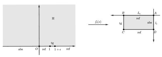
Figure 2. Conformal map

Proposition 5.2.

RBM in $\mathbb{H}$ is mapped to the time-changed RBM in rectangle $ABCD$ by map $f_{\epsilon}$, with reflecting boundaries $AB\cup CD$, absorbing boundaries $AD\cup BC$ and target $BC$.

Proof.

As four points $A,B,C,D$ are Lebesgue null sets we may remove them from consideration and rectangle $ABCD$ could be thought as an analytic simply connected domain. The boundaries are mapped to corresponding boundaries of the rectangle as $f_{\epsilon}$ is injective. Then by proposition 2.11 with reversed direction of $f$ (which also holds, proof is similar) we may conclude. ∎

We observe the following reflection property regarding the RBM in rectangle, which will be useful later.

Proposition 5.3.

Let $z_{0}=x_{0}+iy_{0}$ be a point in the rectangle $ABCD$ such that there exists an open ball $B:=B_{r}(p)\subsetneq ABCD$ where $z_{0}\in B_{r}(p)$, $p\in AB$ and

$$r<\min\{\mathrm{dist}(z_{0},AD),\mathrm{dist}(z_{0},BC)\}.$$

Let $R^{z_{0}}_{t}$ be the RBM in $ABCD$ starts at $z_{0}$ and $\tau_{B}=\inf\{t\geq 0:R^{z_{0}}_{t}\in\partial{B}\cap ABCD\}$. Let $Z^{z_{0}}_{t}=X^{x_{0}}_{t}+iY^{y_{0}}_{t}$ be the standard Brownian motion in $\mathbb{C}$ starts at $z_{0}$ such that both $X^{x_{0}}_{t}$ and $Y^{y_{0}}_{t}$ are independent standard Brownian motions on $\mathbb{R}$ start at $x_{0}$, $y_{0}$, respectively. Let $\tau^{\prime}_{B}=\inf\{t\geq 0:Z^{z_{0}}_{t}\in\partial B\}$, then with probability one, we have

$$R^{z_{0}}_{t\wedge{\tau_{B}}}=X^{x_{0}}_{t\wedge\tau^{\prime}_{B}}-i\left|Y^{y_{0}}_{t\wedge\tau^{\prime}_{B}}\right|.$$

Proof.

By taking minus sign which preserve RBM, the stopped RBM $-R^{z_{0}}_{t\wedge{\tau_{B}}}$ satisfies the stochastic differential equation in the form of (1) as it has normal reflection on $AB$. Let $H^{-z_{0}}_{t}$ be the RBM in $\mathbb{H}$ starts at $-z_{0}$ and that $\tau=\inf\{t\geq 0:H^{-z_{0}}_{t}\in\partial(-B)\cap\mathbb{H}\}$. Then stopped RBM $H^{-z_{0}}_{t\wedge\tau}$ still satisfies the stochastic differential equation in the form of (1). Thus by uniqueness stated in Theorem 2.2 we see that with probability 1, $-R^{z_{0}}_{t\wedge{\tau_{B}}}=H^{-z_{0}}_{t\wedge\tau}$. By Definition 2.8 we can write $H^{-z_{0}}_{t\wedge\tau}=X^{-x_{0}}_{t\wedge\tau^{\prime}_{-B}}+i\left|Y^{-y_{0}}_{t\wedge\tau^{\prime}_{-B}}\right|$ where both $X^{-x_{0}}_{t\wedge\tau^{\prime}_{-B}}$ and $Y^{-y_{0}}_{t\wedge\tau^{\prime}_{-B}}$ are stopped standard Brownian motion in $\mathbb{C}$. By taking minus sign back and notice that with probability 1, $-X^{-x_{0}}_{t\wedge\tau^{\prime}_{-B}}=X^{x_{0}}_{t\wedge\tau^{\prime}_{B}}$ and $-Y^{-y_{0}}_{t\wedge\tau^{\prime}_{-B}}=Y^{y_{0}}_{t\wedge\tau^{\prime}_{B}}$, we have that

$$R^{z_{0}}_{t\wedge{\tau_{B}}}=X^{x_{0}}_{t\wedge\tau^{\prime}_{B}}-i\left|Y^{y_{0}}_{t\wedge\tau^{\prime}_{B}}\right|$$

with probability 1. ∎

so that we may consider the RBM in rectangle as a Brownian motion in strip.

Proposition 5.4.

RBM in rectangle $ABCD$ is equivalent to the standard Brownian motion in the strip $S_{\epsilon}:=\{z\in\mathbb{C}:-L_{\epsilon}<\Re(z)<0\}$ with target at $T_{\epsilon}:=\{z\in\mathbb{C}:\Re(z)=-L_{\epsilon}\}$ and absorbing boundary at Imaginary axis.

Proof.

By equivalent we mean there is an bijective map $h$ between Brownian motion in strip (starts inside rectangle $ABCD$) and RBMs in the rectangle, preserving the corresponding stopping condition. The intuition is shown in figure 3: we may reflect $ABCD$ over its sides with length $L_{\epsilon}$ over and over again to get the strip we need.

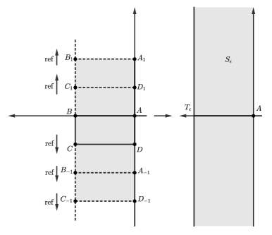
Figure 3. Reflecting rectangle $ABCD$

Define $h_{0}(z)=|\Im{z}|,h_{n}(z)=1-|1-|h_{n-1}(z)|$, and we notice that $h(z)=\lim_{n\to\infty}h_{n}(z)$ exists for all $z$. By proposition 5.3, $h$ works for the bijection. ∎

This implies that

$$\mathbb{P}\left(B^{z_{0}}_{\tau}\in[1,1+\epsilon]\right)=\mathbb{P}\left(f_{\epsilon}\left(B^{z_{0}}\right)_{\tau}\in BC\right)=\mathbb{P}\left(\bar{B}^{f_{\epsilon}\left(z_{0}\right)}_{\tau}\in T_{\epsilon}\right)=\omega_{S}(f_{\epsilon}(z_{0}),T_{\epsilon}).$$

where $\bar{B}$ denotes the Brownian motion in $S_{\epsilon}$ and, abusing notations, $\tau$ denotes the target hitting time of each motion. We can immediately write down the unique harmonic measure $\omega_{S}(f_{\epsilon}(z_{0}),T_{\epsilon})$ in $S_{\epsilon}$:

$$\omega_{S}(f_{\epsilon}(z_{0}),T_{\epsilon})=-\frac{\Re(f_{\epsilon}(z_{0}))}{L_{\epsilon}}.$$

Now plug $z_{0}=Re^{i\theta}$ ($R>0,\theta\in(0,\pi)$) into Christoffel-Schwarz map, after some computation we reach

$$f_{\epsilon}(z_{0})=\frac{e^{-\frac{i\theta}{2}}}{\sqrt{R}}\int_{0}^{1}\frac{dt}{\sqrt{t}\sqrt{t-\frac{e^{-i\theta}}{R}}\sqrt{t-\frac{(1+\epsilon)e^{-i\theta}}{R}}}.$$

By simple Euclidean geometry,

$$\sqrt{\left|t-\frac{e^{-i\theta}}{R}\right|}\sqrt{\left|t-\frac{(1+\epsilon)e^{-i\theta}}{R}\right|}\geq\mathrm{dist}\left(\frac{e^{-i\theta}}{R},\mathbb{R}\right)=\frac{\sin\theta}{R}$$

for $t\in(0,1]$ and thus by Lebesgue Dominated Convergence Theorem we also have that

$$\lim_{\epsilon\downarrow 0}f_{\epsilon}(z_{0})=\int_{0}^{1}\frac{\mathrm{d}t}{\sqrt{t}\left(t-\frac{e^{-i\theta}}{R}\right)}.$$

Now by standard result of $K(x)$ we conclude that $L_{\epsilon}\sim{-\log{\epsilon}}$ as $\epsilon\to 0$. Thus we conclude that

$$\mathbb{P}\left(B^{z_{0}}_{\tau}\in(1,1+\epsilon)\right)\sim\frac{C(z_{0})}{\log\epsilon}$$

as $\epsilon\to 0$, where $C(z_{0})=\Re\left(\lim_{\epsilon\downarrow 0}f_{\epsilon}(z_{0})\right)$. ∎

Corollary 5.5.

Let $\epsilon>0$ and $f_{\epsilon}$ be a conformal map mapping $\mathbb{H}$ into a rectangle $\mathcal{R}$ which can be extended that it maps $0,1,1+\epsilon$ and $\infty$ to corner of $\mathcal{R}$ (then $f_{\epsilon}$ is an uniquely represented Christoffel-Schwarz map). Then for any $z_{0}\in\mathbb{H}$ we have

$$\lim_{\epsilon\to\infty}f_{\epsilon}(z_{0})=C_{1}\int_{0}^{1}\frac{\mathrm{d}t}{\sqrt{t}\left(t-\frac{e^{-i\theta}}{R}\right)}+C_{2}.$$

where $z_{0}=Re^{i\theta}$, $C_{1}$ and $C_{2}$ are the unique constants in Christoffel-Schwarz formula of $f_{\epsilon}$ as described in theorem 4.4.

5.2. Proof of Main Results in $\mathbb{C}$

Now we are ready to proof the main results by explicit computation above. We starts from stronger result.

5.2.1. Proof of Theorem 3.4

Proof.

We introduce some technical lemmas.

Lemma 5.6.

Let $\Omega$ be an analytic simply connected domain and $P$ be a point on $\partial\Omega$. Let $R>0$ be a fixed constant that $S_{R}(P)$ intersects $\partial\Omega$ at non-empty point set $\{A_{t}:t\in I\}$ for some index set $I$. Then $\displaystyle{\sup_{t_{1},t_{2}\in I}\angle{A_{t_{1}}PA_{t_{2}}}}$ is attended by some unique $A_{t_{1}},A_{t_{2}}\in\partial{\Omega}\cap B_{R}(P)$.

Proof.

Firstly notice that $\displaystyle{\angle{A_{t_{1}}PA_{t_{2}}}\leq 2\pi}$ for all $t_{1},t_{2}$ which means the supremum is well-defined and denote it by $s$. We may extract a subsequence $\angle{A^{(n)}_{t_{1}}PA^{(n)}_{t_{2}}}\to s$. As $\Omega$ is an analytic simply connected domain, observe that $\partial{\Omega}\cap B_{R}(P)$ is compact so by choosing a convergence subsequence $\left(A^{(n_{k})}_{t_{1}}\right)_{k\geq 1}$ of $\left(A^{(n)}_{t_{1}}\right)_{n\geq 1}$ and another convergence subsequence $\left(A^{\left(n_{k_{j}}\right)}_{t_{2}}\right)_{j\geq 1}$ of $\left(A^{(n_{k})}_{t_{2}}\right)_{k\geq 1}$, we find $\left(A^{\left(n_{k_{j}}\right)}_{t_{1}},A^{\left(n_{k_{j}}\right)}_{t_{2}}\right)_{j\geq 1}$ converge to some $A_{t_{1}},A_{t_{2}}\in\partial{\Omega}\cap B_{R}(P)$ and $s=\angle{A_{t_{1}}PA_{t_{2}}}$. For uniqueness we just notice that if there exists distinct pairs $(A_{t_{1}},A_{t_{2}})$ and $(A^{\prime}_{t_{1}},A^{\prime}_{t_{2}})$ such that $s=\angle{A_{t_{1}}PA_{t_{2}}}=\angle{A^{\prime}_{t_{1}}PA^{\prime}_{t_{2}}}$, then by simple Euclidean Geometry at least one of angle $\angle{MPN}$ where $M,N\in\{A_{t_{1}},A_{t_{2}},A^{\prime}_{t_{1}},A^{\prime}_{t_{2}}\}$ is greater than $s$. Contradiction. ∎

We call $A_{t_{1}},A_{t_{2}}$ the endpoints of $\partial{\Omega}\cap B_{R}(P)$. Now let $A,D$ be the endpoints of $\mathrm{tg}$ and $B,C$ be the endpoints of $\mathrm{ref}$. We also notice that when $\epsilon$ is very small $\mathrm{tg}$ has only one component. Rigorously speaking, we have the following technical lemma.

Lemma 5.7.

Let $\Omega$ be an analytic simply connected domain, then for all $\epsilon$ small, $B_{P}(\epsilon)\cap\partial\Omega$ has only one connected component.

Proof.

Let $\{C_{t}:t\in I\}$ be the collection of closure of components of $B_{P}(\epsilon)\cap\partial\Omega$ that doesn’t contain $P$. Then as connected component is closed it is compact. So $\mathrm{dist}(P,C_{t})>0$ for all $t\in I$. Now if $\inf\{\mathrm{dist}(P,C_{t}):t\in I\}=0$ then $I$ is infinite and we may take a subsequence $t_{j}$ such that $\mathrm{dist}(P,C_{t_{j}})\to 0$. Now by compactness $\mathrm{dist}(P,C_{t})$ is attended by some point $M_{t}\in C_{t}$, so for $j$ large we have all $M_{t_{j}}$ contained in a small disk $B_{P}(\delta)$ ($\delta<\epsilon$) and thus, as $C_{t_{j}}$ intersect $\partial\Omega$ at two points then their length is greater than $\epsilon-\delta$ for all $j$ large enough. But we have infinitely many such $j$ and thus $\ell(\partial\Omega)\geq\sum_{t}\ell(C_{t})=\infty$, contradiction. So $\inf\{\mathrm{dist}(P,C_{t}):t\in I\}=\xi>0$. Now Take $\epsilon<\xi$ and we are done. ∎

So it is enough to consider one component in $\mathrm{tg}$ and $\epsilon$ very small. Now we can turn to proof the main result. We firstly uniformize our domain. By Riemann Mapping Theorem there is an unique conformal bijection $h$ (extended analytically to boundary) that maps $\Omega$ onto unit disk $\mathbb{D}$ with boundary points $P$ mapped into $X$, $B$ mapped into $Y$ with non-vanishing derivative at $P$ and $B$. Let $f(C)=Z$. This is true because we assume $\Omega$ has an analytic boundary. This process is shown in figure 4.

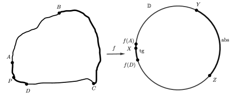
Figure 4. $\Omega$ being mapped into $\mathbb{D}$

Now we can proof the stronger result. Let $f_{1}(z)$ be the extension of $f^{-1}$ beyond $\mathbb{D}$ as $\Omega$ is a analytic simply connected domain (see lemma 7.3). By open mapping theorem image of a neighborhood of $\partial\mathbb{D}$ via $f_{1}$ is an open neighborhood $\Delta$ of $\partial\Omega$. Let fixed $\delta$ so small that $B_{P}(\delta)$ is also contained in $\Delta$. Take $\epsilon<\delta$, then $f_{1}$ is invertible on $B_{P}(\epsilon)$ with holomprohic inverse $g_{1}$ that has derivatives bounded away from $0$. We can get an estimation for lower bound using the univalent map $f_{1}$ which has non-vanishing derivative on $\partial\mathbb{D}$. Also, for any $\eta>0$ we may choose $\eta_{1}$ such that for any $\epsilon<\eta_{1}$, $|g_{1}^{\prime}(z)-g_{1}^{\prime}(P)|\leq\eta$ for all $z\in B_{P}(\epsilon)$. Consider when $\eta<|g^{\prime}_{1}(P)|$ and $\epsilon$ is sufficiently small, then by boundary correspondence, for all $z\in\partial g_{1}(B_{P}(\epsilon))$, $f_{1}(z)\in\partial(B_{P}(\epsilon))$. Consider the line segment joining $z$ and $g_{1}(P)$, let it be $\gamma(\xi)$. Then,

$$\left|z-g_{1}(P)\right|=\int_{\gamma}|(g_{1}\circ f_{1}\circ\gamma)^{\prime}(\xi)|\mathrm{d}\xi\geq(|g_{1}^{\prime}(P)|-\eta)\ell(\gamma)\geq(|g_{1}^{\prime}(P)|-\eta)\epsilon.$$

and we also simultaneously have

$$\left|z-g_{1}(P)\right|\leq\int_{P}^{f_{1}(z)}|g_{1}^{\prime}(\xi)|\mathrm{d}\xi\leq(|g_{1}^{\prime}(P)|+\eta)\mathrm{dist}(f_{1}(z),P)\leq(|g_{1}^{\prime}(P)|+\eta)\epsilon.$$

Now let $M$ be the (unique) mobius transform sending unit disk $\mathbb{D}$ to $\mathbb{H}$ with $g_{1}(P)$ being sent to $1$, $g_{1}(B)$ being sent to $0$ and $g_{1}(D)$ being sent to $\infty$. We do assume that $g_{1}(A)$ being sent to complex number $1-k_{1}(\epsilon)>0$ and $g_{1}(B)$ to $g(D)=1+k_{2}(\epsilon)$ when $\epsilon$ small . Choose $\eta^{\prime}$ small, and by almost the same argument above we could also bound

$$(|M^{\prime}(g_{1}(P))|-\eta^{\prime})(|g_{1}^{\prime}(P)|-\eta)\epsilon\leq|k_{2}(\epsilon)-k_{1}(\epsilon)|\leq(|M^{\prime}(g_{1}(P))|+\eta^{\prime})(|g_{1}^{\prime}(P)|+\eta)\epsilon.$$

for $\epsilon$ small enough. Just as above, choose $T_{\epsilon}(z)=\displaystyle\frac{z}{1-k_{1}(\epsilon)}$ and $T_{\epsilon}\circ M\circ g_{1}$ sends $\Omega$ to $\mathbb{H}$ again but with $A$ to 1 instead, so $B$ is sent to $\displaystyle\frac{1+k_{2}(\epsilon)}{1-k_{1}(\epsilon)}$. Hence

$$\mathbb{P}\left(B^{z_{0}}_{\tau}\in\mathrm{tg}\right)=\mathbb{P}\left(\left(T_{\epsilon}\circ M\circ g_{1}\right)(B^{z_{0}})_{\tau}\in\left(1,\displaystyle\frac{1+h_{2}(\epsilon)}{1-h_{1}(\epsilon)}\right)\right)$$

Remark that $T_{\epsilon}\circ M\circ g_{1}(z_{0})\to M\circ g_{1}(z_{0})$ as $\epsilon\to 0$. As $\eta$, $\eta^{\prime}$ is arbitrary, hence by Theorem 5.1,

$$\mathbb{P}\left(B^{z_{0}}_{\tau}\in\mathrm{tg}\right)\sim-\frac{\Re(M\circ g_{1}(z_{0}))}{\log(|M^{\prime}(g_{1}(P))||g_{1}^{\prime}(P)|\epsilon)}$$

as $\epsilon\downarrow 0$. Hence

$$\mathbb{P}\left(B^{z_{0}}_{\tau}\in\mathrm{tg}\right)\log\epsilon\to-\Re(M\circ g_{1}(z_{0}))$$

as $\epsilon\downarrow 0$. ∎

5.2.2. Proof of Theorem 3.3 in $\mathbb{C}$

Proof.

Our result follows from the following lemma and proof of Theorem 3.4.

Lemma 5.8.

There is an arc of length independent of $\epsilon$ that contained in $f(\mathrm{abs})$.

Proof.

Just a modification of length estimations in proof of Theorem 3.4. ∎

Observe that, if we let $c_{1}$ be an arc contained in $\mathrm{abs}$ and $c_{2}$ be another arc containing $f(\mathrm{abs})$ (for example, such $c_{2}$ can be the arc with endpoints $Y$, $Z$, which does not intersect $f(\mathrm{tg})$). Let us consider the target hitting probability for the absorbing boundary to be $c_{1}$, $f(\mathrm{abs})$ and $c_{2}$, which are $\mathbb{P}_{1}$, $\mathbb{P}_{2}$, $\mathbb{P}_{3}$, respectively, then $\mathbb{P}_{3}\leq\mathbb{P}_{2}\leq\mathbb{P}_{1}$. As by Theorem 3.4 $\mathbb{P}_{3}$ and $\mathbb{P}_{1}$ are comparable to $\displaystyle\frac{1}{\log\epsilon}$ as $\epsilon\downarrow 0$, $\mathbb{P}_{2}$ is as well. ∎

6. Proof of Main Result in General SULD Domains

As we remarked we consider the case when $\epsilon$ is very small. In this case we can localize our domain

6.1. Localization of Domain

Observe that when the RBM particle is near the target the hitting probability is asymptotically irrelevant to the shape of domain.

Without loss of generality let $\mathrm{tg}\in U^{1}$ and let $\mathscr{C}_{1}$, $\mathscr{C}_{2}$ be two fixed $n-1$ dimensional subsets in $U^{1}$ such that $\Phi_{1}(\mathscr{C}_{1})=\partial B_{P}(r_{1})\cap\Phi_{1}(U_{1})$ and $\Phi_{1}(\mathscr{C}_{2})=\partial B_{P}(r_{2})\cap\Phi_{1}(U_{1})$ for some $r_{1}>r_{2}>0$ and that both curves do not intersects $\mathrm{abs}$. As both $\mathscr{C}_{1}$ and $\mathscr{C}_{2}$ are disjoint compact sets their distance is separated and we may assume that any curve $\gamma:[0,1]\to\Omega$ connecting some points on $\mathrm{abs}$ and $P=\gamma(1)$ that only intersects $\mathscr{C}_{1}$ and $\mathscr{C}_{2}$ once for each, intersects $\mathscr{C}_{1}$ at $t_{1}$ and $\mathscr{C}_{2}$ at $t_{2}$ where $t_{1}<t_{2}$ ($\mathscr{C}_{2}$ lies “closer” to $P$ than $\mathscr{C}_{1}$). We let $\tau_{1}=\inf\{t\geq 0:B_{t}^{x_{0}}\in\mathscr{C}_{2}\}$ for $i=1,2$. Let $\mathbb{P}_{1}:=\mathbb{P}(B^{x_{0}}_{\tau}\in\mathrm{tg},B^{x_{0}}_{[\tau_{1},\tau]}\cap\mathscr{C}_{1}=\emptyset)$. We claim the following observation:

Proposition 6.1.

There exists constants $c_{1}$, $c_{2}$ such that

$$c_{1}\mathbb{P}_{1}\leq\mathbb{P}\left(B^{x_{0}}_{\tau}\in\mathrm{tg}\right)\leq c_{2}\mathbb{P}_{1}$$

Proof.

From definition of $\mathbb{P}_{1}$ we immediately have $\mathbb{P}_{1}\leq\mathbb{P}\left(B^{x_{0}}_{\tau}\in\mathrm{tg}\right)$, and notice that

$$\mathbb{P}\left(B^{x_{0}}_{\tau}\in\mathrm{tg}\right)=\mathbb{P}_{1}+\mathbb{P}(B^{x_{0}}_{\tau}\in\mathrm{tg},B^{x_{0}}_{[\tau_{1},\tau]}\cap\mathscr{C}_{1}\neq\emptyset).$$

Since our RBM particle roams outside $\Phi_{1}^{-1}(\overline{B_{P}(r_{1})}\cap\Phi_{1}(U_{1}))$ we have a smaller chance to hit $\mathrm{tg}$ so $\mathbb{P}_{1}\geq\mathbb{P}(B^{x_{0}}_{\tau}\in\mathrm{tg},B^{x_{0}}_{[\tau_{1},\tau]}\cap\mathscr{C}_{1}\neq\emptyset)$. Thus $\mathbb{P}\left(B^{x_{0}}_{\tau}\in\mathrm{tg}\right)\leq 2\mathbb{P}_{1}$. ∎

By strong Markov property,

(3) $$\mathbb{P}\left(B^{x_{0}}_{\tau}\in\mathrm{tg}\right)=\mathbb{P}(\tau_{1}\leq\infty)\times\mathbb{P}\left(B_{\tau}^{B^{x_{0}}_{\tau_{1}}}\in\mathrm{tg}\right)$$

as any RBM hits target will hits $\mathscr{C}_{1}$ by geometrical observation. Now from above proposition for asymptotic behavior we may consider $\mathbb{P}\left(B_{\tau}^{B^{x_{0}}_{\tau_{1}}}\in\mathrm{tg},B^{x_{0}}_{[\tau_{1},\tau]}\cap\mathscr{C}_{1}=\emptyset\right)$. This probability can be interpreted as the probability that the RBM starts at a point $\mathscr{C}_{2}$, roaming in $\Phi_{1}^{-1}(\overline{B_{P}(r_{1})}\cap\Phi_{1}(U_{1}))$ and hits target, which is same as the target hitting probability that our domain is instead the interior of $\Phi_{1}^{-1}(\overline{B_{P}(r_{1})}\cap\Phi_{1}(U_{1}))$ with absorbing boundary $\mathscr{C}_{1}$ and the same target. We can thus localize our domain into interior of $\Phi_{1}^{-1}(\overline{B_{P}(r_{1})}\cap\Phi_{1}(U_{1}))$, which will be denoted by $U^{\prime}$, as shown in figure 5.

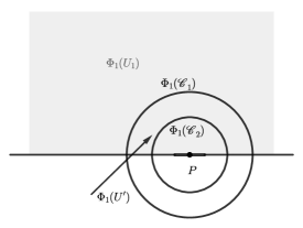
Figure 5. local structure near $P$

6.2. Explicit Computation and Estimation in $U^{\prime}$

We may now turn to some explicit computations and we restrict the RBM in $U^{\prime}$ for now. Now notice that $\Phi_{1}$ maps $\mathscr{C}_{1}$ and $\mathscr{C}_{2}$ into two semi-spheres by their definition. We denote them by $\mathscr{S}_{1}$, $\mathscr{S}_{2}$, respectively. We also define our RBM in $\Omega$ by $\Phi_{1}$ so we may consider the original RBM satisfies $(1)$ and associated assumptions in $\Phi_{1}(U^{1})$.

Now by similar reason as Proposition 5.3 we may reflect $\Phi_{1}(U^{1})\cap\overline{B_{P}(r_{1})}$ along $\mathbb{R}_{0}^{n-1}=\{(0,x_{2},...,x_{n}):x_{i}\in\mathbb{R}\}$ and then the RBM in $\Phi_{1}(U^{1})\cap\overline{B_{P}(r_{1})}$ is equivalent to the Brownian Motion $W_{t}$ stated in equation $(1)$ in $\overline{B_{P}(r_{1})}\setminus\Phi_{1}(\mathrm{tg})$.

Now by adapting the proof in the case of $\mathbb{C}$ with mean value inequality we may assume that there exists constants $k_{1}$, $k_{2}$ depends on $\Phi_{1}$ (hence $\Omega$) such that $B_{P}(k_{1}\epsilon)\cap\mathbb{R}_{0}^{n-1}\subset\Phi_{1}(\mathrm{tg})\subset B_{P}(k_{2}\epsilon)\cap\mathbb{R}_{0}^{n-1}$ for all $\epsilon$ small enough, which allows us to have

(4) $$\mathbb{P}_{k_{1}}\leq\mathbb{P}\left(B_{\tau}^{B^{x_{0}}_{\tau_{1}}}\in\mathrm{tg}\right)\leq\mathbb{P}_{k_{2}}$$

where $B_{t}$ is restricted in $U^{\prime}$ and

$$\mathbb{P}_{k_{i}}:=\mathbb{P}\left(\Phi_{1}(B)_{\tau}^{\Phi_{1}\left(B^{x_{0}}_{\tau_{1}}\right)}\in B_{P}(k_{i}\epsilon)\cap\mathbb{R}_{0}^{n-1}\right)$$

(we have abused notation $\tau$). So now we may turn the problem into the asymptotic hitting probability for the following problem: Given the RBM starts at a point $y_{0}$ on $\mathscr{C}_{1}$, with absorbing boundary $\mathscr{C}_{2}$, target at $B_{P}(k_{i}\epsilon)\cap\mathbb{R}_{0}^{n-1}$ for $i=1,2$, and reflecting boundary at $(B_{P}(r_{1})\setminus B_{P}(k_{i}\epsilon))\cap\mathbb{R}_{0}^{n-1}$. The target hitting probability is $\mathbb{P}_{k_{i}}$ for each $i$.

By reflection $\mathbb{P}_{k_{i}}$ is the probability that the Brownian motion $W^{\Phi_{1}\left(B^{x_{0}}_{\tau_{1}}\right)}_{t}$, where $W_{t}$ is stated in equation $(1)$ and restricted in $\overline{B_{P}(r_{1})}\setminus(B_{P}(k_{i}\epsilon)\cap\mathbb{R}_{0}^{n-1})$ with target $B_{P}(k_{i}\epsilon)\cap\mathbb{R}_{0}^{n-1}$ and absorbing boundary $\partial B_{P}(r_{1})$, hits the target at escaping time of $B_{P}(r_{1})$.

Now we consider the sphere $\partial B_{P}(k_{1}\epsilon)$. Then let

$$\tau_{2}=\inf\left\{t\geq 0:W^{\Phi_{1}\left(B^{x_{0}}_{\tau_{1}}\right)}_{t}\notin B_{P}(r_{1})\setminus\overline{B_{P}(k_{1}\epsilon)}\right\}$$

writing $\Phi_{1}\left(B^{x_{0}}_{\tau_{1}}\right)=y_{0}$ , again by strong Markov Property we have that

(5) $$\mathbb{P}_{k_{1}}=\mathbb{P}\left(W^{y_{0}}_{\tau_{2}}\in\partial B_{P}(k_{1}\epsilon)\right)\times\mathbb{P}\left(W_{\tau}^{W^{y_{0}}_{\tau_{2}}}\in B_{P}(k_{1}\epsilon)\cap\mathbb{R}_{0}^{n-1}\right).$$

Now we observe again that $\mathbb{P}\left(W^{y_{0}}_{\tau_{2}}\in\partial B_{P}(k_{1}\epsilon)\right)$ is the probability of the Brownian Motion $W^{\Phi_{1}\left(B^{x_{0}}_{\tau_{1}}\right)}_{t}$ inside the $n$ dimensional open annulus $B_{P}(r_{1})\setminus\overline{B_{P}(k_{1}\epsilon)}$ with absorbing boundary at $\partial B_{P}(r_{1})$ and target at $\partial B_{P}(k_{1}\epsilon)$. Now we may explicitly write out the solution to this target hitting probability. Since we know that the target hitting probability $\mathbb{P}\left(W^{y_{0}}_{\tau_{2}}\in\partial B_{P}(k_{1}\epsilon)\right)=u_{1}(y_{0})$ satisfies the Dirichlet problem

$$\begin{cases}\Delta u_{1}(y)=0&\text{ if }y\in B_{P}(r_{1})\setminus\overline{B_{P}(k_{1}\epsilon)}\\ u_{1}(y)=1&\text{ if }y\in\partial B_{P}(k_{1}\epsilon)\\ u_{1}(y)=0&\text{ if }y\in\partial B_{P}(r_{1})\end{cases}$$

as the solution to this problem is unique, and thus we may easily verify that

$$\mathbb{P}\left(W^{y_{0}}_{\tau_{2}}\in\partial B_{P}(k_{1}\epsilon)\right)=u_{1}(y_{0})=\frac{G_{n,P}(y_{0})-G_{n,P}(P+\bm{r_{1}})}{G_{n,P}(P+\bm{k_{1}\epsilon})-G_{n,P}(P+\bm{r_{1}})}.$$

where $\bm{r_{1}}=(r_{1},0,0,...,0)\in\mathbb{R}^{n}$ and $\bm{k_{1}\epsilon}=(k_{1}\epsilon,0,0,...,0)\in\mathbb{R}^{n}$, is the solution to the above problem.

Now we need to estimate $\mathbb{P}\left(W_{\tau}^{y_{1}}\in B_{P}(k_{1}\epsilon)\cap\mathbb{R}_{0}^{n-1}\right)$ where $W^{y_{0}}_{\tau_{2}}=y_{1}$. We claim the following estimation:

Proposition 6.2.

There exists a constant $c_{3}^{(1)}=c_{3}^{(1)}(k_{1})>0$ such that

$$\mathbb{P}\left(W_{\tau}^{y_{1}}\in B_{P}(k_{1}\epsilon)\cap\mathbb{R}_{0}^{n-1}\right)\geq c_{3}^{(1)}$$

for any $y_{1}\in\partial B_{P}(k_{1}\epsilon)$ and small $\epsilon$.

Proof.

Consider probability that $W_{\tau}^{y_{1}}\in B_{P}(k_{1}\epsilon)\cap\mathbb{R}_{0}^{n-1}$ but without hitting $\partial B_{y_{1}}(4k_{1}\epsilon)$ for $\epsilon$ so small that $\overline{B_{P}(5k_{1}\epsilon)}\subset B_{P}(r_{1})$. We notice that if we let $H^{y_{1}}_{t}$ be the same Brownian motion as $W^{y_{1}}_{t}$ in $B_{P}(r_{1})\setminus(B_{P}(k_{1}\epsilon)\cap\mathbb{R}_{0}^{n-1})$ but with absorbing boundary $\partial B_{y_{1}}(4k_{1}\epsilon)$ and target $B_{P}\left(\displaystyle{k_{1}\epsilon}\right)\cap\mathbb{R}_{0}^{n-1}$ instead, we will have

$$\mathbb{P}\left(W_{\tau}^{y_{1}}\in B_{P}(k_{1}\epsilon)\cap\mathbb{R}_{0}^{n-1}\right)\geq\mathbb{P}\left(H_{\tau}^{y_{1}}\in B_{P}\left(\displaystyle{k_{1}\epsilon}\right)\cap\mathbb{R}_{0}^{n-1}\right).$$

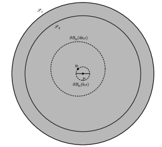
Figure 6. Local structure near $P$

By shifting and rescaling invariance of Brownian motion, let

$$Z_{t}:=\frac{H^{y_{1}}_{t}-y_{1}}{4k_{1}\epsilon}$$

be another (non standard) Brownian motion started at $0$, roams inside $B_{0}(1)$, with original target of $H^{y_{1}}_{t}$ being shifted and rescaled to a $n-1$ dimensional open ball with diameter $\displaystyle\frac{1}{2}$ (which will be denoted by $\mathrm{tg}^{\prime}$) and absorbing boundary being shifted and rescaled to $\partial B_{0}(1)$. Let $\tau_{3}=\inf\{t\geq 0:Z_{t}\notin B_{0}(1)\setminus\mathrm{tg}^{\prime}\}$ Then we have

$$\mathbb{P}\left(H_{\tau}^{y_{1}}\in B_{P}\left(\displaystyle{k_{1}\epsilon}\right)\cap\mathbb{R}_{0}^{n-1}\right)=\mathbb{P}(Z_{\tau_{3}}\in\mathrm{tg}^{\prime}).$$

We notice that $\mathrm{dist}(0,\mathrm{tg}^{\prime})<\displaystyle\frac{1}{4}$. Consider the $n-1$ dimensional cube $Q_{1}$ inscribed in $\mathrm{tg}^{\prime}$ and we notice that there exists a positive constant $c_{4}$ such that it only depends on $n-1$ and the side length of $Q_{1}$ is ${c_{4}}$. Now consider building up another $n$ dimensional cube $Q_{2}$ with one face exactly $Q_{1}$ and $0$ lies in same side of $Q_{2}$ compare to $\mathbb{R}^{n-1}_{0}$. Then $Q_{2}$ is well defined and lies inside $B_{0}(1)$. Let the center of $Q_{2}$ be $Q$ and construct sphere $\partial B_{Q}\left(\displaystyle\frac{c_{4}}{4}\right)$, as shown in figure 7.

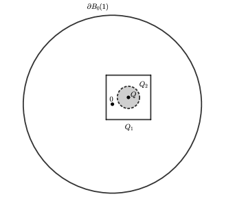
Figure 7. $Q$, $Q_{1}$ and $Q_{2}$

Let $\mathbb{P}_{3}$ be the probability that $Z_{t}$ hits $\partial B_{Q}\left(\displaystyle\frac{c_{4}}{4}\right)$ before hitting $\partial B_{0}(1)$. Then as $c_{4}$ is independent of $\epsilon$ there exists constant $c_{5}>0$ only depends on $n$ and $k_{1}$ such that $\mathbb{P}_{3}\geq c_{5}$. Let $\mathbb{P}_{4}$ be the probability that starts on a point on $\partial B_{Q}\left(\displaystyle\frac{c_{4}}{4}\right)$ and exits $Q_{2}$ at $Q_{1}$. Then by rescaling invariance we also see there exists $c_{6}>0$ that also only depends on $n$ and $k_{1}$ such that $\mathbb{P}_{4}\geq c_{6}$. So

$$\mathbb{P}(Z_{\tau_{3}}\in\mathrm{tg}^{\prime})\geq\mathbb{P}_{3}\times\mathbb{P}_{4}\geq c_{5}c_{6}>0.$$

Thus we have

$$\mathbb{P}\left(W_{\tau}^{y_{1}}\in B_{P}(k_{1}\epsilon)\cap\mathbb{R}_{0}^{n-1}\right)\geq c_{3}^{(1)}:=c_{5}c_{6}.$$

∎

We may obtain the same result for the case of $k_{2}$.

6.3. Proof of Main Result

Now we may finish the proof. By $(4)$ and above proof we have

$$u_{i}(y_{0})c^{(i)}_{3}\leq\mathbb{P}_{k_{i}}\leq u_{i}(y_{0})$$

for $i=1,2$. So by $(2),(3)$ and proposition we proofed in 6.1 we have

$$c_{1}c_{3}^{(1)}\mathbb{P}(\tau_{1}<\infty)u_{1}(y_{0})\leq\mathbb{P}\left(B^{x_{0}}_{\tau}\in\mathrm{tg}\right)\leq c_{2}\mathbb{P}(\tau_{1}<\infty)u_{2}(y_{0}).$$

We note that $\mathbb{P}\left(\tau_{1}<\infty\right)>0$ as position of $\mathscr{C}_{2}$ is independent of $\epsilon$. We also notice that

$$u_{i}(y_{0})=\begin{cases}\displaystyle\frac{r_{1}^{2-n}-r_{2}^{2-n}}{r_{1}^{2-n}-(k_{i}\epsilon)^{2-n}}&\text{ if }n\in\mathbb{N}\backslash\{1,2\}\\ \displaystyle\frac{\log(r_{2})-\log(r_{1})}{\log(k_{i}\epsilon)-\log(r_{1})}&\text{ if }n=2\end{cases}$$

So that let $\epsilon\to 0$ we have $u_{i}$ is comparable with general Newtonian potential and thus the main result is proven.

7. Appendix: Proofs of technical details

Proposition 7.1.

Suppose $\mathscr{V}=\left\{V^{0},V^{1},...\right\}$ is another cover of $\Omega$ defined in 2.4 and $(\Psi_{k})_{k\geq 1}$ be another collection of associated maps. Suppose for some $k$ and $m$ that $V_{m}\cap U_{k}$ is non-empty. Then the transition map

$$\Phi_{k}\circ(\Psi_{m})^{-1}:\Psi_{m}(V_{m}\cap U_{k})\to\Phi_{k}(V_{m}\cap U_{k})$$

maps process $\Psi_{m}(X^{x}_{t})$ to the process $\Phi_{k}(X^{x}_{t})$.

Proof.

Notice that for $X^{x}_{t}$ inside domain $\Omega$, it satisfies Stochastic differential equation $\mathrm{d}X^{x}_{t}=\mathrm{d}W_{t}$. Write $\Psi_{m}=f=(f^{1},f^{2},...,f^{n})$ and $\Phi_{k}=g=(g^{1},...,g^{n})$, $W_{t}=(W^{1}_{t},...,W^{n}_{t})$ where $W^{i}_{t}$ are independent standard 1 dimensional Brownian motion. Apply Itô’s formua,

(6) $$\mathrm{d}f^{i}(X_{t})=\left(\sum^{n}_{k=1}\frac{\partial f^{i}}{\partial x_{k}}\mathrm{d}W^{k}_{t}\right)+\frac{1}{2}\Delta f^{i}\mathrm{d}t+\mathbf{1}_{\partial\Phi_{k}(U_{k})\cap\overline{\mathbb{H}}}(f(X_{t}))\nabla f^{i}(X_{t})\cdot\gamma\mathrm{d}\xi_{t}$$

where $\delta_{1i}=0$ for $i\neq 1$ and $1$ for $i=1$. We abbreviate starting position to make our equation clean. We also abbreviate

$$R(f,i,\xi_{t},X_{t})=\mathbf{1}_{\partial\Phi_{k}(U_{k})\cap\overline{\mathbb{H}}}(f(X_{t}))\nabla f^{i}(X_{t})\cdot\gamma\mathrm{d}\xi_{t}$$

where $\gamma$ is the unit vector field normal to boundary of $V_{m}\cap U_{k}$. Write $f(X_{t})$ as $F_{t}=(F^{1}_{t},F^{2}_{t},...,F^{n}_{t})$, we need to show that $g\circ f^{-1}$ maps process $F_{t}$ to same process in $g(V_{m}\cap U_{k})$. Apply Itô’s formula again we have

(7) $$\mathrm{d}\left(g\circ\left(f^{-1}\right)\right)^{i}(F_{t})=\sum_{k=1}^{n}\frac{\partial\left(g\circ\left(f^{-1}\right)\right)^{i}}{\partial x_{k}}\mathrm{d}F_{t}^{k}+\frac{1}{2}\sum^{n}_{k,m=1}\frac{\partial^{2}\left(g\circ\left(f^{-1}\right)\right)^{i}}{\partial x_{k}\partial x_{m}}\mathrm{d}\langle F^{m},F^{k}\rangle_{t}$$

plug in (6) and rearrange (7) we have

$$\mathrm{d}\left(g\circ\left(f^{-1}\right)\right)^{i}(F_{t}) =\sum_{k=1}^{n}\sum_{p=1}^{n}\frac{\partial g^{i}}{\partial x_{p}}\frac{\partial\left(f^{-1}\right)^{p}}{\partial x_{k}}\sum_{j=1}^{n}\frac{\partial f^{k}}{\partial x_{j}}\mathrm{d}W_{t}^{j}$$

$$+\frac{1}{2}\left(\sum_{k,m=1}^{n}\sum_{a=1}^{n}\frac{\partial^{2}\left(g\circ\left(f^{-1}\right)\right)^{i}}{\partial x_{k}\partial x_{m}}\frac{\partial f^{k}}{\partial x_{a}}\frac{\partial f^{m}}{\partial x_{a}}+\Delta f^{k}\sum_{p=1}^{n}\frac{\partial g^{i}}{\partial x_{p}}\frac{\partial\left(f^{-1}\right)^{p}}{\partial x_{k}}\right)\mathrm{d}t$$

$$+\sum^{n}_{j=1}\frac{\partial(g\circ f^{-1})^{i}}{\partial x_{j}}R(f,j,\xi_{t},X_{t})$$

where $\left(f^{-1}\right)^{p}$ is interpreted as the $p^{\mathrm{th}}$ component of $f^{-1}$. Notice that by written in multiplication form of Jacobian matrix the first term on RHS is just $\sum^{n}_{k=1}\frac{\partial g^{i}}{\partial x_{k}}\mathrm{d}W^{k}_{t}$ and second term is $\frac{1}{2}\Delta g^{i}\mathrm{d}t$. We also note that

$$\gamma\cdot\sum^{n}_{j=1}\frac{\partial(g\circ f^{-1})^{i}}{\partial x_{j}}\nabla f^{k}=\gamma\cdot\nabla g^{i},$$

which implies

$$\sum^{n}_{j=1}\frac{\partial(g\circ f^{-1})^{i}}{\partial x_{j}}R(f,j,\xi_{t},X_{t})=R(g,i,\xi_{t},X_{t})$$

Thus we have verified that

$$\mathrm{d}g^{i}(X^{x}_{t})=\sum^{n}_{k=1}\frac{\partial g^{i}}{\partial x_{k}}\mathrm{d}W^{k}_{t}+\frac{1}{2}\Delta g^{i}\mathrm{d}t+R(g,m,i,\xi_{t},X_{t})=\mathrm{d}\left(g\circ\left(f^{-1}\right)\right)^{i}(F_{t})$$

so consistency follows. ∎

Proposition 7.2.

$\mathbb{D}$ is a SULD. More over, any domain $\Omega$ defined in Definition 2.7 is a SULD.

Proof.

See Appendix, Choose $\displaystyle{f_{j}(z)=(i)^{j}\frac{z-i}{z+i}}$ for $j=1,2,3,4$. and we note that each $f_{j}$ is conformal between an open neighborhood of a subset $\mathbb{H}^{\prime}$ of $\mathbb{H}$ around $0$, denoted by $\mathbb{H}^{\prime\prime}$, and an open neighborhood of $\mathbb{D}\cap(i)^{j+1}\mathbb{H}$, denoted by $\mathbb{D}_{j}^{\prime}$, $0$ is sent to $-i^{j}$ and each $\mathbb{D}^{\prime}_{j}=i\mathbb{D}^{\prime}_{j-1}$. With out loss of generality we may assume that $d=\inf\{|x-y|:x\in\partial\mathbb{D}\cap-\mathbb{H},y\in\partial\mathbb{D}^{\prime}_{1}\}>0$ and that each $f_{i}$ is holomorphic on some neighborhood of $\overline{\mathbb{H}^{\prime\prime}}$ with a holomorphic inverse. Now for $z\in\partial\mathbb{D}\cap(i)^{j+1}\mathbb{H}$ we take $B^{j}_{z}=B^{j}_{z}\left(\frac{d}{2}\right)$ and by compactness of $\partial\mathbb{D}$ we can find $(B^{j}_{z_{k}}:1\leq k\leq n_{j})$ such that $\partial\mathbb{D}\cap(i)^{k+1}\mathbb{H}\subset\cup^{n_{j}}_{k=1}B^{j}_{z_{k}}.$ Put $\mathscr{U}=\{\mathbb{D}\}\cup\cup^{4}_{j=1}\{B^{j}_{z_{k}}:1\leq k\leq n_{j}\}$ each map $\Phi_{k}$ be the correspondent $(f_{j})^{-1}$. So $\mathbb{D}$ satisfies properties 1-3. Now as each $f_{j}$ is holomorphic on neighborhood of $\overline{\mathbb{H}^{\prime\prime}}$ we conclude that $\left|\left(f^{-1}_{j}\right)^{\prime}\right|$ is bounded above by positive constants $d_{1}$ independent of $j$ as we only have finitely many $f_{j}$. So

$$\left|\left(f^{-1}_{j}\right)^{\prime}(x)-\left(f^{-1}_{j}\right)^{\prime}(y)\right|=\left|\int^{x}_{y}\left(f^{-1}_{j}\right)^{\prime}(z)\mathrm{d}z\right|\leq d_{1}|x-y|$$

and on the other hand, notice that in particular $(i)^{j}\notin\mathbb{D}_{j}^{\prime}$ so there is a $d_{2}>0$ such that $\mathrm{dist}((i)^{j},\mathbb{D}_{j}^{\prime})\geq d_{2}$. Now

$$\left|f^{-1}_{j}(x)-f^{-1}_{j}(y)\right|=\left|\frac{ix+(i)^{j+1}}{(i)^{j}-x}-\frac{iy+(i)^{j+1}}{(i)^{j}-y}\right|=\left|\frac{2(x-y)}{((i)^{j}-x)((i)^{j}-y)}\right|\geq\frac{2}{d^{2}_{2}}|x-y|.$$

so $f^{-1}_{j}$ satisfies a Lipchitz condition. As we only have 4 $j$ we have the uniform Lipchitz condition. Also from here all partial derivative are nicely bounded by total derivative of $f^{-1}_{j}$. By Cauchy-Riemann Equation we see $J_{j}J_{j}^{T}=c\mathbb{I}$ where $c=|(f^{-1}_{j})^{\prime}|^{2}>0$, $J_{j}$ is Jacobian of $f^{-1}_{j}$ and $\mathbb{I}$ is the $2\times 2$ identity matrix. Also $f^{-1}_{j}$ are all harmonic, so property 4 is satisfied. Thus $\mathbb{D}$ is a SULD. For the case of general $\Omega$ in Definition 2.7, by Riemann mapping theorem we may choose a conformal bijection $f$ maps $\mathbb{D}$ onto $\Omega$. Now we introduce a lemma

Lemma 7.3.

Let $f$ be a conformal bijection between $\mathbb{D}$ and $\Omega$ where $\Omega$ is defined in 2.7. Then we may extend $f$ to a conformal bijection $F$ between $\Omega^{\prime}$, an open neighborhood of $\Omega$ and $\mathbb{D}^{\prime}$, an open neighborhood of $\mathbb{D}$, and $F$ agree with $f$ on $\mathbb{D}$. [13] (Theorem 2.25)

So we may extend $f$ to be such $F$ and for each $x\in\partial\Omega$ we have $\overline{B_{x}(r_{x})}\subset\Omega^{\prime}$. Then as $\partial\Omega$ is compact we can find an integer $N$ such that $\partial\Omega=\cup^{n}_{k=1}B_{x_{k}}(r_{x_{k}})$. Let $g$ be the inverse of $F$. Write $B_{x_{k}}(r_{x_{k}})=B_{k}$ and consider $B_{j,m,k}=g(B^{j}_{z_{m}})\cap B_{k}$ with associated map $\Phi_{j,m,k}=g\circ f_{j}^{-1}$. Then take $\mathscr{U}={\Omega}\cup\left(\cup^{4}_{j=1}\cup^{n_{j}}_{m=1}\cup^{n}_{k=1}B_{j,m,k}\right)$ we see $\Omega$ satisfies properties 1-3. Now as $g^{-1}$ is also conformal its derivative is bounded by some constant $c_{j,m,k}$ on $\overline{B_{j,m,k}}$ and so by similar argument as (7) we have

$$|x-y|=|g^{-1}(g(x))-g^{-1}(g(y))|\leq c_{j,m,k}|g(x)-g(y)|\leq\max_{j,m,k}c_{j,m,k}|g(x)-g(y)|.$$

Thus

$$\frac{2}{d^{2}_{2}}|x-y|\leq\left|f^{-1}_{j}(x)-f^{-1}_{j}(y)\right|\leq\left(\max_{j,m,k}c_{j,m,k}\right)\left|\left(g\circ f^{-1}_{j}\right)(x)-\left(g\circ f^{-1}_{j}\right)(y)\right|$$

and as $g^{\prime}$ is bounded on each $\overline{B_{j,m,k}}$ we can similarly also find constant $d_{3}>0$ such that

$$\left|\left(g\circ f^{-1}_{j}\right)(x)-\left(g\circ f^{-1}_{j}\right)(y)\right|\leq d_{3}\left|f^{-1}_{j}(x)-f^{-1}_{j}(y)\right|\leq d_{3}d_{1}|x-y|.$$

Together by same reasons listed in about proof that $\mathbb{D}$ satisfies property 4, we see property 4 is satisfied and thus $\Omega$ is a SULD. ∎

Proposition 7.4.

Suppose $\Omega$ and $\Omega^{\prime}$ are two simply connected open subset of $\mathbb{H}$ and $B^{z_{0}}_{t}$ is the RBM in $\mathbb{H}$ where $z_{0}\in\Omega$ with the associated local time process $\xi^{z_{0}}_{t}$. Let $f$ be a conformal automorphism of $\mathbb{H}$. Let $\tau_{\Omega}=\inf\{t\geq 0:B^{z_{0}}_{t}\in\partial\Omega\}$. Then with probability one, $(f(B^{z_{0}}_{t}),t\in[0,\tau))$ is equal to the time-changed RBM in $\mathbb{H}$.

Proof.

We may assume that $B^{z_{0}}_{t}$ is written in the form in the proof of proposition 2.2 with associated $\xi^{z_{0}}_{t}$ also given. Write in clean notation $B^{z_{0}}_{t}=(\tilde{X^{z_{0}}_{t}},Y^{z_{0}}_{t})$ where $Y^{z_{0}}_{t}$ is the standard 1 dimensional Brownian motion independent of $\tilde{X^{z_{0}}_{t}}$. We also write $X^{z_{0}}_{t}$ for the standard 1 dimensional Brownian motion generates $\tilde{X^{z_{0}}_{t}}$. Write $f(z_{0})=w_{0}$. As conformal automorphism of $\mathbb{H}$ takes the form

$$f(z)=\frac{az+b}{cz+d}\qquad a,b,c,d\in\mathbb{R},ad-bc=1$$

We have that $f^{\prime}(z)=\displaystyle\frac{1}{(cz+d)^{2}}$ and note that it is positive on $\mathbb{R}\setminus\{\frac{-d}{c}\}$. We may remove point $\frac{-d}{c}$ out of consideration as it has zero Lebesgue measure. Consider the associated process $(Y^{w_{0}}_{t},\Xi^{w_{0}}_{t})$ defined by $Y^{w_{0}}_{t}=f\left(B_{t}^{z_{0}}\right)$ and

$$\Xi^{w_{0}}_{t}=\int^{t}_{0}f^{\prime}(B_{t})\mathrm{d}\xi_{s}.$$

It suffice to check that $f(B^{z_{0}}_{t})-\mathbf{1}_{\partial\mathbb{H}}\left(f(B^{z_{0}}_{t})\right)\Xi^{w_{0}}_{t}$ is a time changed complex Brownian motion. Write $f(z)=u(x,y)+iv(x,y)$ where $z=a+bi$. Apply Itô’s formula, note that $f$ is harmonic:

$$\mathrm{d}\left(u(\tilde{X}_{t},Y_{t})-\mathbf{1}_{\partial\mathbb{H}}\left(f(B^{z_{0}}_{t})\right)\Xi_{t}\right)$$

$$=\frac{\partial u}{\partial x}\left(\tilde{X}_{t},Y_{t}\right)\mathrm{d}\tilde{X}_{t}+\frac{\partial u}{\partial y}\left(\tilde{X}_{t},Y_{t}\right)\mathrm{d}Y_{t}-\mathbf{1}_{\partial\mathbb{H}}\left(f(B^{z_{0}}_{t})\right)\frac{\partial u}{\partial x}\mathrm{d}\Xi_{t}$$

$$=\frac{\partial u}{\partial x}\left(\tilde{X}_{t},Y_{t}\right)\left(\mathrm{d}X_{t}+\mathbf{1}_{\partial\mathbb{H}}\left(B^{z_{0}}_{t}\right)\mathrm{d}\xi_{t}\right)+\frac{\partial u}{\partial y}\left(\tilde{X}_{t},Y_{t}\right)\mathrm{d}Y_{t}-\mathbf{1}_{\partial\mathbb{H}}\left(f(B^{z_{0}}_{t})\right)\frac{\partial u}{\partial x}\mathrm{d}\Xi_{t}$$

$$=\frac{\partial u}{\partial x}\left(\tilde{X}_{t},Y_{t}\right)\mathrm{d}X_{t}+\frac{\partial u}{\partial y}\left(\tilde{X}_{t},Y_{t}\right)\mathrm{d}Y_{t},$$

Similarly

$$\mathrm{d}\left(v(\tilde{X}_{t},Y_{t})-\mathbf{1}_{\partial\mathbb{H}}\left(f(B^{z_{0}}_{t})\right)\Xi_{t}\right)=\frac{\partial v}{\partial x}\left(\tilde{X}_{t},Y_{t}\right)\mathrm{d}X_{t}+\frac{\partial v}{\partial y}\left(\tilde{X}_{t},Y_{t}\right)\mathrm{d}Y_{t}.$$

Write $\displaystyle\tilde{u}=u(\tilde{X}_{t},Y_{t})-\mathbf{1}_{\partial\mathbb{H}}\left(f(B^{z_{0}}_{t})\right)\Xi_{t}$ and $\displaystyle\tilde{v}=v(\tilde{X}_{t},Y_{t})-\mathbf{1}_{\partial\mathbb{H}}\left(f(B^{z_{0}}_{t})\right)\Xi_{t}$. Then their quadratic variation satisfies

$$\langle\tilde{u}\rangle_{t}=\langle\tilde{v}\rangle_{t}=\int_{0}^{t}\left|f^{\prime}\left(B_{s}\right)\right|^{2}ds$$

with zero covariation. Let

$$\sigma(t)=\inf\left\{s\geq 0:\int_{0}^{s}\left|f^{\prime}\left(B_{u}\right)\right|^{2}du>t\right\}$$

and set $\tilde{B}^{w_{0}}_{t}=\tilde{u}\left(B^{z_{0}}_{\sigma(t)}\right)+i\tilde{v}\left(B^{z_{0}}_{\sigma(t)}\right)$. By the Dubins-Schwarz theorem, $\tilde{B}^{w_{0}}_{t}$ is a complex Brownian motion. ∎

8. Acknowledgement

I would like to express my deepest gratitude to prof. Dmitry Belyaev as my supervisor of this summer project. He advised me the topic of this project and supervised me throughout the project.

References

- [1] K. Burdzy and Z.-Q. Chen, “Reflecting random walk in fractal domains,” The Annals of Probability, vol. 41, no. 4, Jul. 2013. [Online]. Available: http://dx.doi.org/10.1214/12-AOP745
- [2] R. F. Anderson and S. Orey, “Small random perturbation of dynamical systems with reflecting boundary,” Nagoya Mathematical Journal, vol. 60, pp. 189–216, 1976.
- [3] Q. Hu, Y. Wang, and X. Yang, “The hitting time density for a reflected brownian motion,” Computational Economics, vol. 40, pp. 1–18, 06 2012.
- [4] A. Chaigneau and D. S. Grebenkov, “Effects of target anisotropy on harmonic measure and mean first-passage time,” Journal of Physics A: Mathematical and Theoretical, vol. 56, no. 23, p. 235202, May 2023. [Online]. Available: http://dx.doi.org/10.1088/1751-8121/acd313
- [5] S. Redner, A Guide to First-Passage Processes. Cambridge University Press, 2001.
- [6] D. S. Grebenkov and A. T. Skvortsov, “Mean first-passage time to a small absorbing target in three-dimensional elongated domains,” Phys. Rev. E, vol. 105, p. 054107, May 2022. [Online]. Available: https://link.aps.org/doi/10.1103/PhysRevE.105.054107
- [7] P. Grandits, “Asymptotics of the hitting probability for a small sphere and a two dimensional Brownian motion with discontinuous anisotropic drift,” Bernoulli, vol. 27, no. 2, pp. 853 – 865, 2021. [Online]. Available: https://doi.org/10.3150/20-BEJ1257
- [8] A. E. Lindsay, A. J. Bernoff, and M. J. Ward, “First passage statistics for the capture of a brownian particle by a structured spherical target with multiple surface traps,” Multiscale Modeling & Simulation, vol. 15, no. 1, pp. 74–109, 2017. [Online]. Available: https://doi.org/10.1137/16M1077659
- [9] G. F. Lawler, Conformally invariant processes in the plane. American Mathematical Soc., 2008, no. 114.
- [10] B. Øksendal, “Brownian motion and sets of harmonic measure zero.” 1981.
- [11] R. F. Bass and P. Hsu, “The semimartingale structure of reflecting brownian motion,” Proceedings of the American Mathematical Society, vol. 108, no. 4, pp. 1007–1010, 1990. [Online]. Available: http://www.jstor.org/stable/2047960
- [12] E. M. Stein and R. Shakarchi, Complex analysis. Princeton University Press, 2010, vol. 2.
- [13] D. Beliaev, Conformal Maps and Geometry. WORLD SCIENTIFIC (EUROPE), 2019. [Online]. Available: https://www.worldscientific.com/doi/abs/10.1142/q0183
- [14] B. Øksendal, Diffusions: Basic Properties. Berlin, Heidelberg: Springer Berlin Heidelberg, 2003, pp. 115–140. [Online]. Available: https://doi.org/10.1007/978-3-642-14394-6_7