FuseFormer: A Transformer for
Visual and Thermal Image Fusion

Abstract

Image fusion is the process of combining images from different sensors into a single image that incorporates all relevant information. The majority of state-of-the-art image fusion techniques use deep learning methods to extract meaningful features; however, they primarily integrate local features without considering the image’s broader context. To overcome this limitation, Transformer-based models have emerged as a promising solution, aiming to capture general context dependencies through attention mechanisms. Since there is no ground truth for image fusion, the loss functions are structured based on evaluation metrics, such as the structural similarity index measure (SSIM). By doing so, we create a bias towards the SSIM and, therefore, the input visual band image. The objective of this study is to propose a novel methodology for image fusion that mitigates the limitations associated with using evaluation metrics as loss functions. Our approach integrates a transformer-based multi-scale fusion strategy, which adeptly addresses both local and global context information. This integration not only refines the individual components of the image fusion process but also significantly enhances the overall efficacy of the method. Our proposed method follows a two-stage training approach, where an auto-encoder is initially trained to extract deep features at multiple scales at the first stage. For the second stage, we integrate our fusion block and change the loss function as mentioned. The multi-scale features are fused using a combination of Convolutional Neural Networks (CNNs) and Transformers. The CNNs are utilized to capture local features, while the Transformer handles the integration of general context features. Through extensive experiments on various benchmark datasets, our proposed method, along with the novel loss function definition, demonstrates superior performance compared to other competitive fusion algorithms. Furthermore, we show the effectiveness of the proposed fusion strategy with an ablation and performance analysis. The source code is also available.

I Introduction

Image fusion is a powerful technique in the context of computer vision that involves combining information from multiple images taken at different wavelengths or bands to create a single, comprehensive representation. The primary objective of image fusion is to extract and integrate complementary details and features from each input image, resulting in a more informative and enhanced composite image. The fusion of images from different bands holds immense significance and due to fact that its widely used in night vision and thermal imaging, remote sensing and multiple spectre imaging, last but not least multi-modal medical imaging.

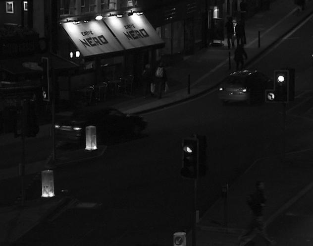
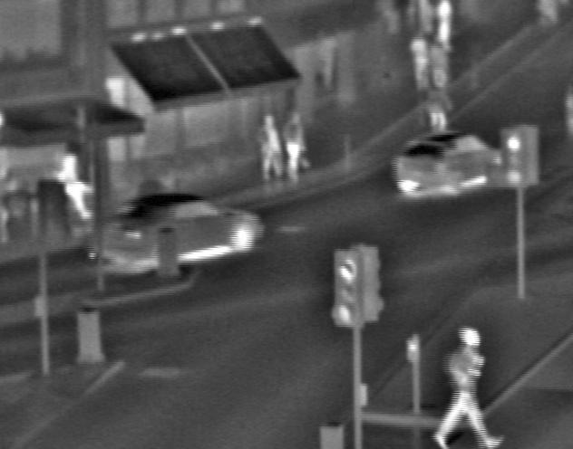
(a) Visual Band, Thermal Band Images

(b) Our Output Image, SwinFusion[1] Image

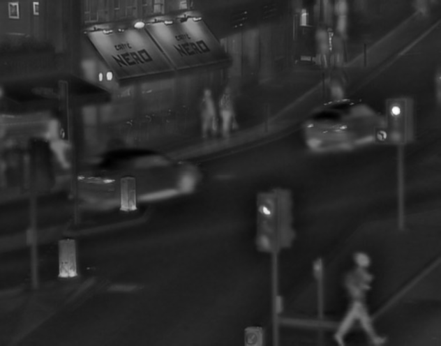
(c) M3FD[2] - RFN-Nest[3] Output Images

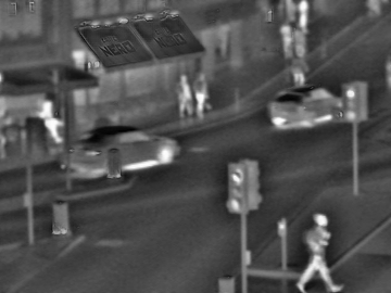
(d) IFT[4], DenseFuse[5] Output Images

Figure 1: Night Vision Enhancement Comparison with SoTA Method

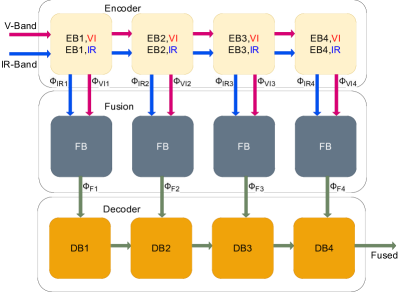
Figure 2: Proposed Method’s Block Diagram

Research on image fusion dates back to 1989 with Toet et al. [6]. Traditional image fusion algorithms have been extensively investigated in the existing literature, but they are not without drawbacks. A significant concern with these methods lies in the incorporation of handcrafted steps, leading to suboptimal outcomes. With the advent of the deep learning era, attempts have been made to address this issue using Convolutional Neural Networks (CNNs) [7], Autoencoders [5, 8, 9, 10, 11, 12], and Generative Adversarial Networks (GANs) [13, 14, 15, 16, 17, 18, 19, 20]. However, these approaches exhibit limitations in effectively capturing long-range dependencies. To mitigate this challenge, Transformers [21, 22, 23, 4, 24, 1, 25, 26, 1, 27] have been employed to tackle image fusion problems. Despite this advancement, a primary drawback persists: the reliance on evaluation metrics such as Structural Similarity Index (SSIM) [28] as the main component of the loss function. This practice, while yielding satisfactory quantitative results, often leads to poor qualitative outcomes in the fused images. The main contributions of this work can be summarized as follows:

• We propose a novel fusion method, called FuseFormer, that utilizes a Transformer-CNN fusion block with a unique loss function by taking both input images into account. By doing so, it mitigates the gap between quantitative and qualitative results.

• The proposed method utilizes Transformers to capture global context and combines the results with local features from Convolutional Neural Networks (CNNs).

• The proposed method is evaluated on multiple fusion benchmark datasets, where we achieve competitive results compared to existing fusion methods.

II Related Work

The RGB and infrared image fusion domain has undergone extensive research, traversing from Traditional Fusion Algorithms to cutting-edge Transformer-based models [29, 30, 31, 32, 33]. In the early 1990s, methods like Sparse Representation and Multi-scale Transformation were explored, each with its inherent limitations. Traditional algorithms, relying on handcrafted steps, faced challenges in adaptability and time complexity [29, 30, 31, 32, 33]. The scarcity of labeled datasets for RGB-IR fusion prompted a shift towards unsupervised scenarios, guiding our exploration of Performance Evaluation metrics.

With the advent of deep learning, learning-based algorithms became predominant, categorized by learning methods, loss functions, and the use of labeled datasets [34, 5, 8, 9, 13]. CNN-based approaches, both supervised and unsupervised, exhibited success in feature extraction for image fusion, yet challenges persisted in scenarios with significant differences in factors like illumination or resolution [34]. Autoencoder-based algorithms, utilizing neural networks for dimensionality reduction, showcased advancements in works such as DenseFuse, Raza et al., and Fu et al. [5, 8, 9].

GAN-based methods, introduced by Goodfellow et al., focused on unsupervised fusion, integrating attention mechanisms and residual connections for improved performance [13, 18, 35]. While these approaches demonstrated promise, challenges persisted in effectively handling the inherent differences between fused and source images.

A transformative shift in RGB-IR image fusion occurred with the introduction of Transformer-based algorithms in 2021 [21, 22, 23]. These methodologies, driven by the self-attention mechanism, marked a paradigm shift by efficiently managing long-range dependencies in images. Innovative designs, such as multiscale fusion strategies and dual transformer approaches, were introduced, emphasizing the seamless integration of Transformers with traditional methods [4, 26, 24, 36]. Unsupervised Transformer-based techniques, reliant on loss functions, eliminated the need for labeled data but posed challenges in methodological evaluations [4, 26]. Ongoing research explores diverse Transformer integrations, Transformer-CNN combinations, and the utilization of auxiliary information to further enrich the fusion process [4, 26, 24, 36]. The integration of deep learning methods has not only enhanced feature extraction capabilities but has also paved the way for more adaptive and robust solutions in the challenging methodologies of image fusion. Due to the vastness of the subject, it is impractical to encompass all relevant studies here. For a comprehensive overview, readers are directed to Zhang et al. [37] which provides insights into the broader landscape of RGB-IR image fusion research, including advancements, methodologies, and challenges.

III Methodology

Image fusion can be decomposed into three key components: the feature extractor, feature fuser, and image reconstructor. The feature extractor is responsible for extracting multilevel features from input images. Subsequently, the feature fuser merges these extracted features into unified feature maps for each level. These consolidated features play a crucial role in the final image reconstruction, orchestrated by the image reconstructor.

In terms of analogy, the feature extractor corresponds to the encoder in autoencoders, while the image reconstructor aligns with the decoder in autoencoders. The feature fuser leverages both Convolutional Neural Networks (CNNs) and transformers, with CNNs adeptly managing local features and transformers overseeing global contexts. This merge enhances the fusion process, ultimately aiming to improve accuracy.

Our approach involves a two-stage training process. In the initial stage, we train an autoencoder, originally derived from RFN-Nest [3] as illustrated in Figure 3. Subsequently, in the second stage, we train our fusion block, depicted in Figure 4, in conjunction with the previously trained autoencoder.

III-A Autoencoder Training

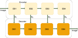
(a) Block Diagram

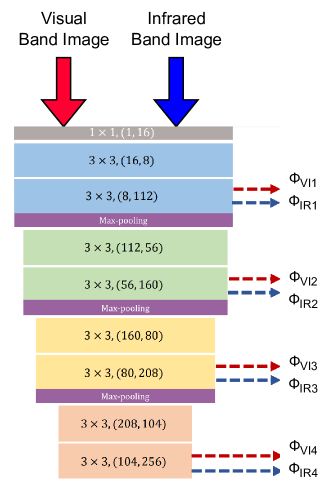
(b) RFN-Nest [3] Encoder

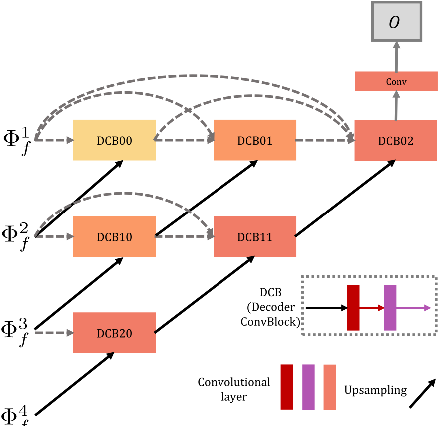
(c) RFN-Nest [3] Decoder

Figure 3: Autoencoder Training

The initial phase of the training process involves instructing the encoder network to capture multi-scale deep features. Concurrently, the decoder network is also trained to reconstruct the input image, utilizing the aforementioned multi-scale deep features. The training framework of the auto-encoder network is depicted in Figure 3. These extracted multi-scale deep features are then fed into the decoder network for the purpose of reconstructing the input image. Leveraging short cross-layer connections ensures the comprehensive utilization of the multi-scale deep features in the image reconstruction process.

The loss function, denoted as $L_{ae}$, serves as the training criterion for the autoencoder network and is defined in the subsequent manner:

$$L_{ae}=L_{pixel}+\alpha L_{SSIM}$$ (1)

The terms $L_{pixel}$ and $L_{SSIM}$ refer to the pixel loss and the structural similarity (SSIM) loss, respectively, computed between the input and output images. The parameter $\alpha$ represents the trade-off parameter governing the balance between the contributions of $L_{pixel}$ and $L_{SSIM}$ meanwhile also it handles the order of magnitude difference in the overall loss function in Eq 1.

$$L_{\text{pixel}}=\left\lvert\left\lvert\text{image}_{\text{output}}-\text{image}_{\text{input}}\right\rvert\right\rvert_{F}^{2}$$ (2)

$L_{pixel}$ is defined in Eq 2. where $\left\lvert\left\lvert\text{.}\right\rvert\right\rvert_{F}$ denotes Frobenius norm. $L_{pixel}$ ensures that the reconstructed image closely resembles the original input image at the individual pixel level, imposing a constraint on the fidelity of pixel-wise information in the reconstruction process. This constraint helps to maintain fine-grained details and accuracy in the reconstructed image, ensuring that it retains the essential characteristics of the input image at a granular level.

The second term in Eq 1 is the SSIM loss $L_{SSIM}$ is defined as in Eq 3:

$$L_{SSIM}=1-SSIM(image_{output},image_{input})$$ (3)

where $SSIM(.)$ is the structural similarity measure [28] which quantifies the structural similarity of the two images. The structural similarity between Input and Output is constrained by $L_{SSIM}$. The Structural Similarity Index (SSIM) is a widely used metric for evaluating the similarity between two images. It aims to capture not only the pixel-wise differences but also the structural information and perceptual quality of the images.

The Structural Similarity Index ($SSIM$) is a metric that quantifies the similarity between two images, yielding values within the range of -1 to 1. A $SSIM(\bigodot,\bigodot)$ value of 1 denotes perfect similarity, indicating that the images share same characteristics in terms of luminance, contrast, and structure. Conversely, a value close to -1 signifies a substantial dissimilarity between the images. Notably, the $SSIM(\bigodot,\bigodot)$ index demonstrates a strong correlation with human perception of image quality, making it widely employed in diverse image processing and computer vision applications [28].

The $SSIM$ constrains its output to the range of $[-1,1]$, which consequently bounds the $L_{SSIM}$ loss function (as defined in Eq. (3)) to the interval $[0,2]$. In this context, lower values of $L_{SSIM}$ indicate better performance with respect to $SSIM$. In contrast, the $L_{pixel}$ loss is unbounded. To balance the impact of both $L_{pixel}$ and $L_{SSIM}$ during training, the trade-off parameter $\alpha$ in Eq. (1) governs their relative magnitudes.

In short, the autoencoder depicted in Figure 3 is subjected to training using the MS-COCO dataset [38] and the RoadScene dataset [39]. The training process is guided by the loss function presented in Eq. (1).

III-B Fusion Block Training

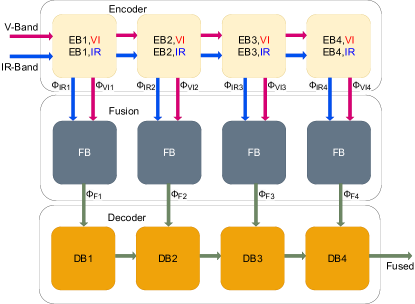
(a) Block Diagram

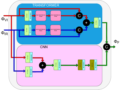
(b) Fusion Block

Figure 4: Fusion Block Training

After successfully extracting multi-scale multi-level features in first stage, see Figure 3, the aim in the second stage training is to merge the features from two separate images: visible band and infrared band images. In this stage, the outputs from separate encoders are then merged into a single multi-scale feature map with fusion block depicted in Figure 4 per scale. This fusion process, which lays on the hearth of this research, is a crucial step as it combines diverse features from different bands, enhancing the feature representation. It allows the model to leverage the strengths of each band, thereby improving the overall effectiveness of the feature extraction process.

Following the fusion, the resulting multi-scale feature maps are subsequently decoded, leading to the reconstruction of the original image, as depicted in Figure 4. Decoding phase reconstructs an image that encapsulates the combined information from both bands. In essence, the reconstructed image, though visually similar to the input images, carries a much richer set of features, potentially paving the way for more accurate subsequent analyses or processes.

In the fusion block, Conventional Convolutional Neural Network (CNN) based techniques facilitate image fusion through the merge of local features. However, a significant limitation inherent to these methods is their lack of consideration for the global context and long range dependencies. In an attempt to overcome this limitation, transformer-based models have been introduced, which leverage the attention mechanism to effectively model the global context.

The first stage of this training protocol necessitates the use of an auto-encoder to extract deep, multi-scale features. In the subsequent stage, these multi-scale features are blended via a fusion strategy that innovatively combines CNNs with Transformers. Comprising a CNN and a transformer branch, the combined fusion blocks capably capture both local and global context features. This method’s success lies in its ability to leverage the strengths of both CNNs and Transformer models, providing a comprehensive view of an image by capturing both local and global contexts. The strategy’s robustness, combined with its efficiency, heralds a new direction for further developments in the field of image fusion. Used combined fusion block details can be seen at Figure 4(b).

The fusion block is characterised by its dual-branch design, which consists of a spatial branch and a transformer branch. The spatial branch integrates convolution layers and a bottleneck layer, specifically tailored to distil local feature representations. Conversely, the transformer branch employs an axial attention-based transformer block to capture the global context embedded within the input data.

While designing the loss function, current researches continue with the same loss defined as in Eq 1. Only single input image, visible band image in general, and the output fused image is used in this loss function. Skipping the unused input image, infrared band image in general, yields a overfitting towards to the used input image. It can be explained as:

• $L_{pixel}=0$ if and only if the input and output image is identical.

• $L_{ssim}=0$ if and only if the input and output image is identical by definition of $SSIM(\bigodot,\bigodot)$.

Therefore, a unique loss function is deployed that leverages both input images. The fusion loss function $L_{fuse}$, as in $L_{ae}$, can be formulated as in Eq 4:

$$L_{fuse}=L_{pixel}+\alpha L_{ssim}$$ (4)

This fusion loss function aims to balance the contribution from pixel-level losses, denoted as $L_{feature}$, and structural similarity losses, $L_{ssim}$, modulated by a trade-off factor, $\alpha$ which handles the difference of order of magnitude for losses. To ensure $L_{fuse}=0$ in Eq 4 corresponds to an optimal fusion scenario, the definitions of $L_{ssim}$ and $L_{feature}$ must be updated as shown in Eq 6 and Eq 5 respectively. While re-defining the losses, the following constraints need to be considered:

1. The fused image should have a higher resemblance to the visual band image while maintaining the global context from the infrared band image almost identical to the visual band image. As a result, $L_{ssim}$ must be computed for both input visual and infrared band images, ideally but not necessarily favoring the visual band image.

2. The pixel values of the fused image should closely match the visual band image due to its compatibility with human vision. Hence, $L_{feature}$ must be calculated on both input visual and infrared band images.

The SSIM loss $L_{ssim}$ is then redefined as:

$$L_{ssim}=\left[1-SSIM(I_{f},I_{v})\right]^{2}+\left[1-SSIM(I_{f},I_{i})\right]^{2}$$ (5)

The redefined $L_{ssim}$ is capable of measuring the similarity of the fused image to both visual and infrared images, and is limited to the interval $(0,8]$.

The pixel-wise loss $L_{feature}$ can be formulated as:

$$L_{feature}=\sum_{m=1}^{M}\omega^{m}\left\lvert\left\lvert\phi_{f}^{m}-\left(\omega_{vi}\phi_{vi}^{m}+\omega_{ir}\phi_{ir}^{m}\right)\right\rvert\right\rvert_{F}^{2}$$ (6)

Here, $M$ refers to the number of scales for deep feature extraction, while $f$, $vi$, and $ir$ denote the fused image, the input visual band image, and the input infrared band image respectively. $\omega^{m}$, $\omega_{vi}$, and $\omega_{ir}$ represent trade-off parameters employed to harmonize the magnitudes of the losses. $\phi_{x}^{m}$ corresponds to the feature maps of $imagex$, which could be either the input or output feature maps of the fusion block, as depicted in Figure 4.

This loss function restricts the fused deep features to preserve significant structures, thereby enriching the fused feature space with more conspicuous features and preserving detailed information.

IV Results

The model training process involved the utilization of three distinct datasets: MS-COCO [38] for autoencoder training in first stage, RoadScene [40] for integration of fusion strategies in second stage, and TNO [41] for comparative analysis. To ensure an unbiased and comprehensive evaluation, a partitioning approach was employed, dividing each dataset into 80%, 10%, and 10% subsets, respectively assigned to the training, testing, and validation sets.

For the hardware components, an NVIDIA RTX 3060Ti with 16GB of memory, paired with an Intel i9 10th generation CPU, was utilized. During the comparison of models, the following metrics were widely used for the evaluation: Entropy (En)[42],Sum of the Correlations of Differences (SCD)[43], Mutual Information (MI)[44],Structural Similarity Index Metric (SSIM)[28].

TABLE I: Loss Functions Comparison

Method	Entropy[42]$\uparrow$	SCD[43]$\downarrow$	MI[44]$\uparrow$	SSIM[28]$\uparrow$
Proposed $L_{fuse}$ in Eq 4	4.536	5.433	1.591	0.884
$L_{ae}$ as $L_{fuse}$ Exp	4.559	6.466	0.552	0.879
RFN-Nest[3]	4.729	7.062	0.602	0.541

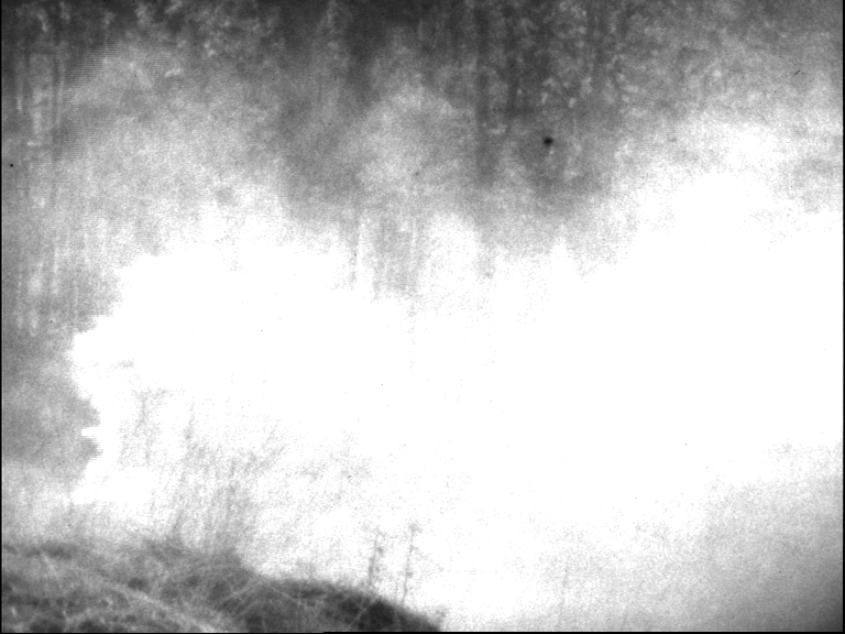
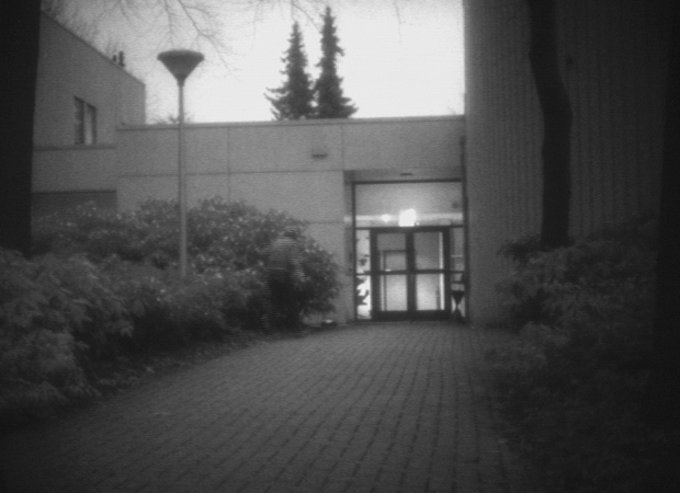
(a) Visual Band Images

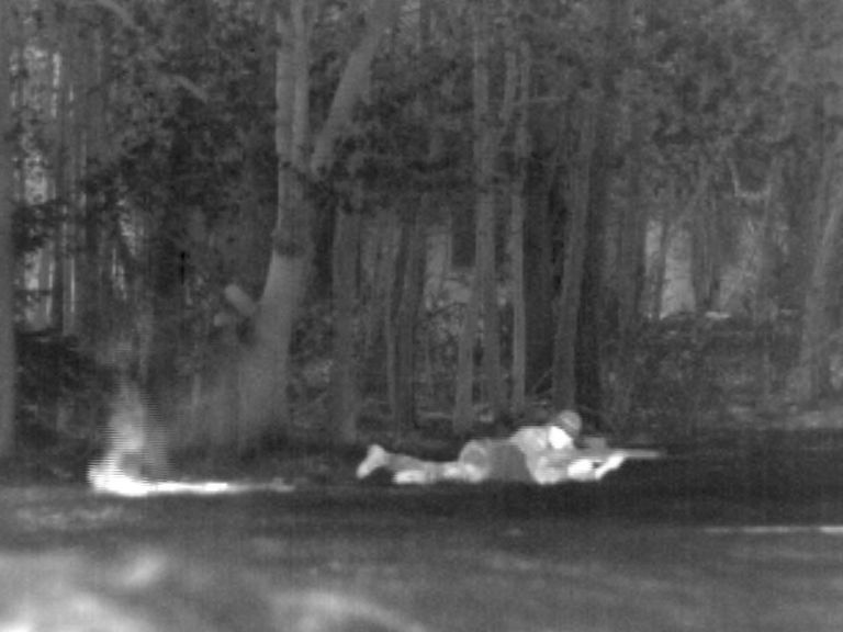
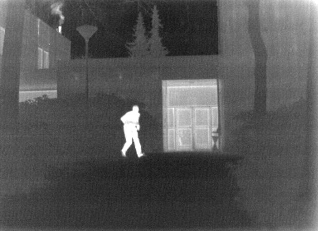
(b) Infrared Band Images

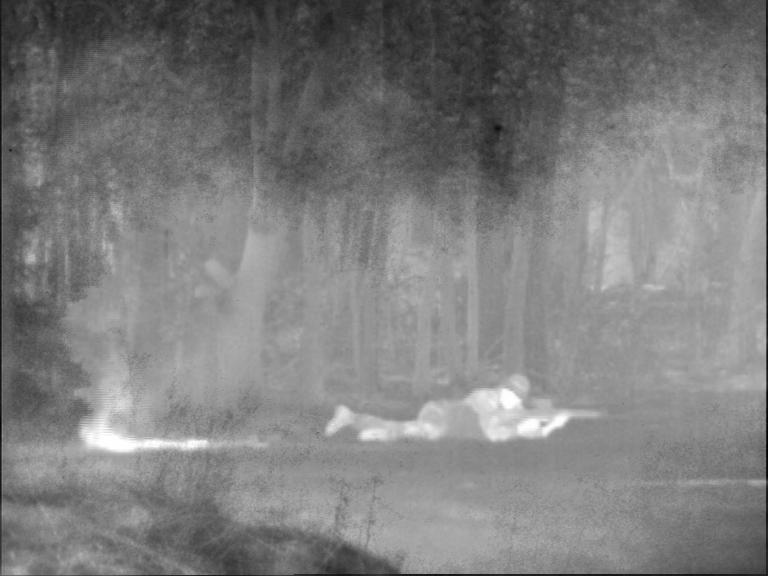
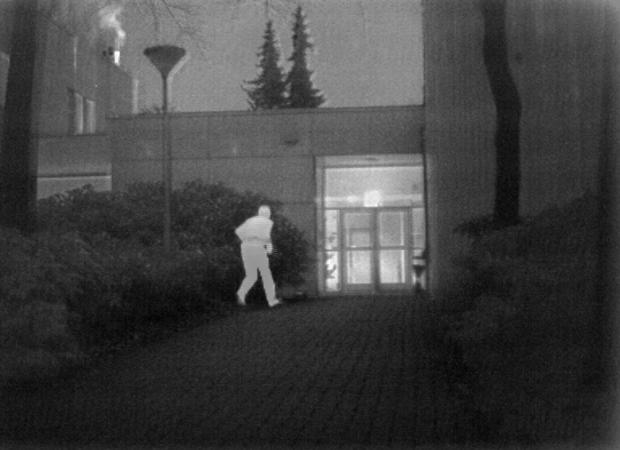
(c) Model With New $L_{fuse}$ Loss Output Images

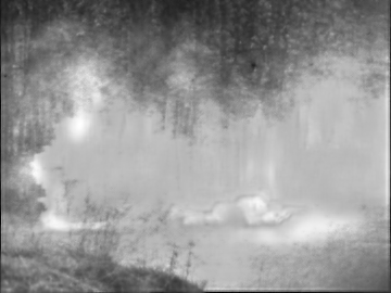
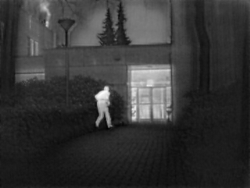
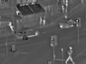
(d) Model With $L_{fuse}=L_{ae}$ Loss Output Images

Figure 5: Loss Functions Comparison

In Table I, the impact of redefining the loss function is systematically examined. Reference results from RFN-Nest [3] are provided since the autoencoder is inherited from RFN-Nest. Despite considering not only the visible band image in the redefined $L_{ssim}$, as depicted in Eq 5, the resulting structural similarity index ($SSIM$) of the visible band image and the fused image surpasses that of the original loss function component $L_{ssim}$, detailed in Eq 3. The redefinition of $L_{ssim}$ not only enhances quantitative results but also improves qualitative outcomes, as illustrated in Figure 5.

(a) Visual Band Images

(b) Infrared Band Images

(c) Our Output Images

(d) SwinFusion[1] Output Images

Figure 6: Comparison with SoTA

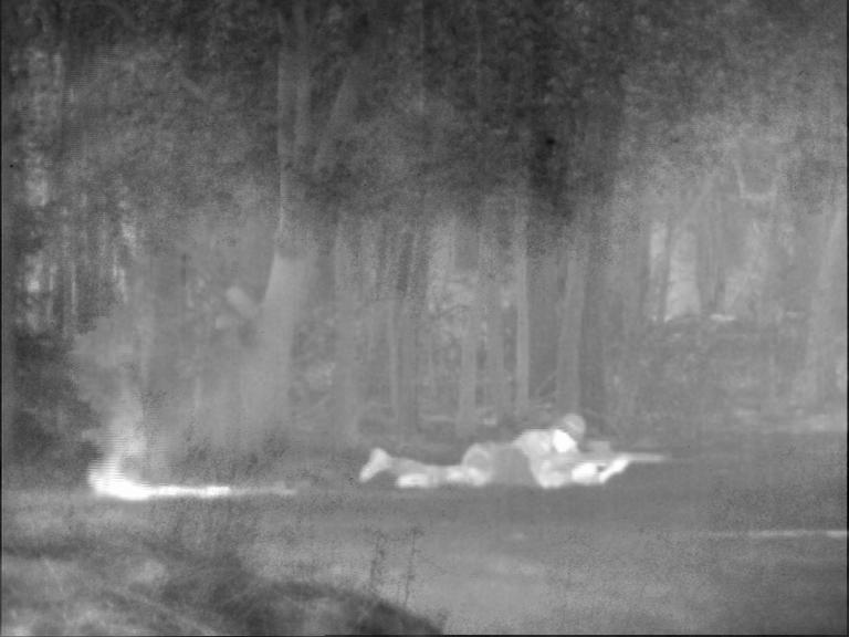
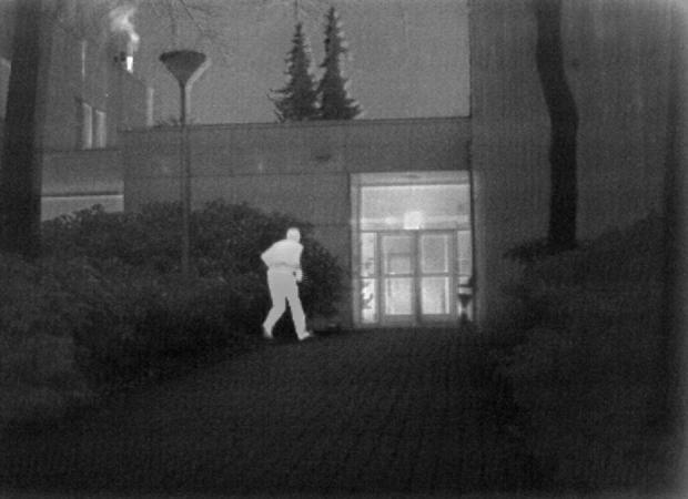
(a) M3FD[2] Output Images

(b) IFT[4] Output Images

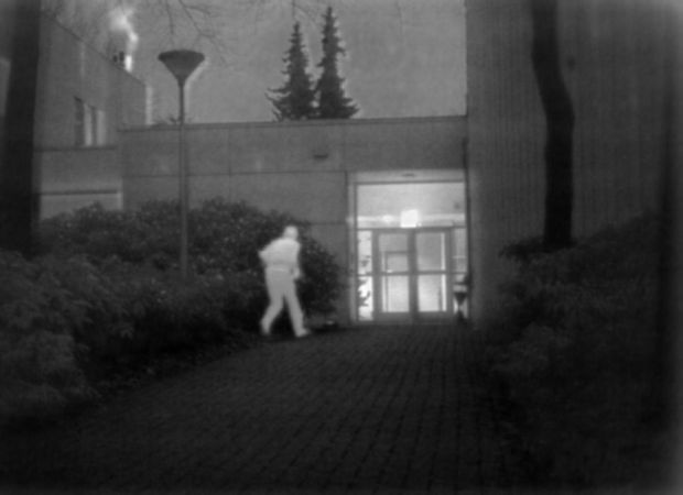
(c) RFN-Nest[3] Output Images

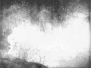
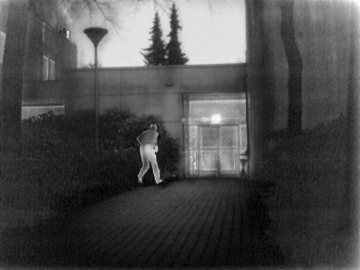
(d) DenseFuse[5] Output Images

Figure 7: Comparison with SoTA cont’d

TABLE II: Comparison with SoTA

Method	Entropy[42]$\uparrow$	SCD[43]$\downarrow$	MI[44]$\uparrow$	SSIM[28]$\uparrow$
Ours	4.536	5.433	1.591	0.884
SwinFusion[1]	4.605	6.760	0.804	0.690
M3FD[2]	4.625	6.858	0.742	0.659
IFT[4]	4.644	6.864	0.684	0.630
DenseFuse[5]	4.724	6.455	0.853	0.588
RFN-Nest[3]	4.729	7.062	0.602	0.541

In Table II, FuseFormer is systematically compared with state-of-the-art (SoTA) methods in a quantitative manner. Simultaneously, a qualitative comparison is conducted through the examination of Figures 6 and 7. The ordering of methods in Table 5 is based on the structural similarity index (SSIM) [28]. Despite variations in the claims made by the authors of the referenced papers, the utilization of the TNO inference approach resulted in the compilation presented in Table II.

The comprehensive evaluation, encompassing both Table II and Figures 6 and 7, establishes FuseFormer as superior both qualitatively and quantitatively across nearly all metrics.

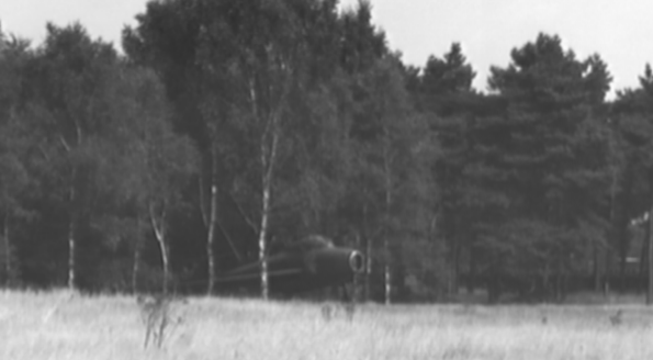
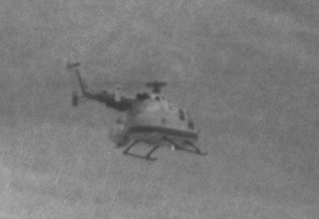
(a) Visual Band Images

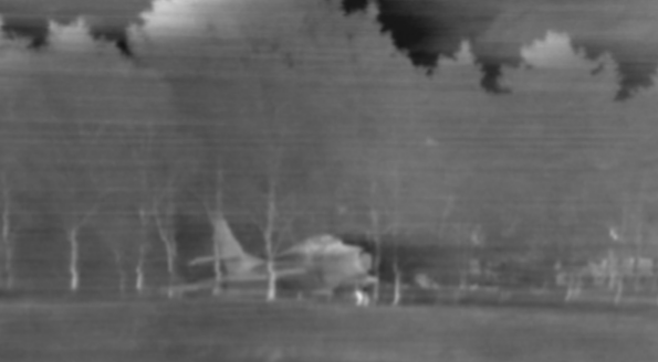
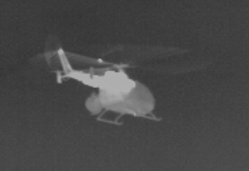
(b) Infrared Band Images

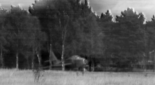
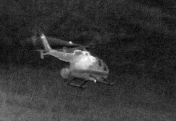
(c) Our Output Images

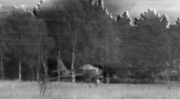
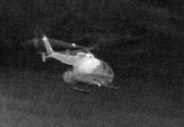
(d) SwinFusion[1]Output Images

Figure 8: Night Vision Enhancement

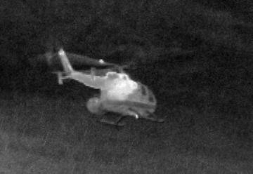
(a) M3FD[2] Output Images

(b) IFT[4] Output Images

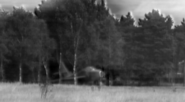
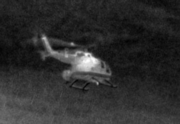
(c) RFN-Nest[3] Output Images

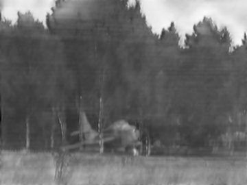
(d) DenseFuse[5] Output Images

Figure 9: Night Vision Enhancement cont’d

As a practical example of using infrared-visible band images, we selected suitable images from the TNO dataset for night vision applications. In Figures 8 and 8, the input visible and infrared images represent instances of night vision scenarios. This specific example is chosen to effectively demonstrate the long-range dependencies and global context present in such images.The images in the second and third columns predominantly depict scenes captured under low-light conditions. Although, at a quick qualitative glance, the differences between the images may seem subtle, a closer examination reveals nuanced distinctions. Turning our attention to Table I, a thorough evaluation indicates that our proposed method consistently produces superior results. In comparison to state-of-the-art (SoTA) techniques, our method shows significant improvements across nearly every evaluated performance metric.

TABLE III: Model Tuning Results: Improvement Rate

Criteria	Initial V	Optimized V	Improvement (%)
Learning Rate	$1\times 10^{-4}$	$1\times 10^{-6}$	7.64%
Batch Size	2	4	3.8%
Transformer Layers	8	12	18.15%
Attention Mech	Self	Axial	N/A%

In this paper, also model tuning experiments are made and the results are given in Table III. For model tuning, affect of changing learning rate, batch size, transformer layers and attention mechanisim are investigated. According to Table IV, changing the number of layers on Transformer side from 8 to 12 improves the resulting SSIM. Due to nature of Transformers, this improvements trades off a huge computation resource and increases the convergence time quadratic. According to Table V, as expected, changing the batch size does not affect the model performance much. Considering the Transformer’s huge computation need, smaller batch sizes comes with a trade off of increased training time and smaller computation power. According to Table VI, changing the learning rate, especially adaptively changing during the training, improves the quality of resulting model. While starting with larger learning rate value, decreasing the learning rate towards to the end improves the convergence.

TABLE IV: Model Tuning Results: Transformer Layers

Experiment	Entropy[42]$\uparrow$	SCD[43]$\downarrow$	MI[44]$\uparrow$	SSIM[28]$\uparrow$
$T_{12}$	4.533	6.152	1.346	0.846
$T_{10}$	4.535	6.335	1.232	0.824
$T_{8}$	4.587	6.657	0.874	0.719

TABLE V: Model Tuning Results: Batch Size

Experiment	Entropy[42]$\uparrow$	SCD[43]$\downarrow$	MI[44]$\uparrow$	SSIM[28]$\uparrow$
$B_{4}$	4.542	6.478	1.130	0.746
$B_{2}$	4.587	6.657	0.874	0.719

TABLE VI: Model Tuning Results: Learning Rate

Experiment	Entropy[42]$\uparrow$	SCD[43]$\downarrow$	MI[44]$\uparrow$	SSIM[28]$\uparrow$
$LR_{1e-6}$	4.553	6.551	1.032	0.774
$LR_{1e-5}$	4.570	6.603	0.948	0.747
$LR_{1e-4}$	4.587	6.657	0.874	0.719

V Conclusion

In this paper, we proposed FuseFormer, a transformer based visible-infrared band image fusion network, where we developed a novel fusion strategy with a novel loss function that contributes from both input images and takes global context into account. In the dual-branch fusion strategy, a CNN and a transformer branches are introduced to fuse both local and global features. The proposed method is evaluated on multiple fusion benchmark datasets where we achieve competitive results compared to the existing fusion methods.

References

- [1] J. Ma, L. Tang, F. Fan, J. Huang, X. Mei, and Y. Ma, “Swinfusion: Cross-domain long-range learning for general image fusion via swin transformer,” IEEE/CAA Journal of Automatica Sinica, vol. 9, no. 7, pp. 1200–1217, 2022.
- [2] J. Liu, X. Fan, Z. Huang, G. Wu, R. Liu, W. Zhong, and Z. Luo, “Target-aware dual adversarial learning and a multi-scenario multi-modality benchmark to fuse infrared and visible for object detection,” in Proceedings of the IEEE/CVF Conference on Computer Vision and Pattern Recognition, pp. 5802–5811, 2022.
- [3] H. Li, X.-J. Wu, and J. Kittler, “Rfn-nest: An end-to-end residual fusion network for infrared and visible images,” Information Fusion, vol. 73, pp. 72–86, 2021.
- [4] V. Vs, J. M. J. Valanarasu, P. Oza, and V. M. Patel, “Image fusion transformer,” in 2022 IEEE International Conference on Image Processing (ICIP), pp. 3566–3570, IEEE, 2022.
- [5] H. Li, X.-j. Wu, and T. S. Durrani, “Infrared and visible image fusion with resnet and zero-phase component analysis,” Infrared Physics & Technology, vol. 102, p. 103039, 2019.
- [6] A. Toet, L. J. Van Ruyven, and J. M. Valeton, “Merging thermal and visual images by a contrast pyramid,” Optical engineering, vol. 28, no. 7, pp. 789–792, 1989.
- [7] Y. Zhang, Y. Liu, P. Sun, H. Yan, X. Zhao, and L. Zhang, “Ifcnn: A general image fusion framework based on convolutional neural network,” Information Fusion, vol. 54, pp. 99–118, 2020.
- [8] A. Raza, H. Huo, and T. Fang, “Pfaf-net: Pyramid feature network for multimodal fusion,” IEEE Sensors Letters, vol. 4, no. 12, pp. 1–4, 2020.
- [9] Y. Fu and X.-J. Wu, “A dual-branch network for infrared and visible image fusion,” in 2020 25th International Conference on Pattern Recognition (ICPR), pp. 10675–10680, IEEE, 2021.
- [10] L. Jian, X. Yang, Z. Liu, G. Jeon, M. Gao, and D. Chisholm, “Sedrfuse: A symmetric encoder–decoder with residual block network for infrared and visible image fusion,” IEEE Transactions on Instrumentation and Measurement, vol. 70, pp. 1–15, 2020.
- [11] Z. Wang, Y. Wu, J. Wang, J. Xu, and W. Shao, “Res2fusion: Infrared and visible image fusion based on dense res2net and double nonlocal attention models,” IEEE Transactions on Instrumentation and Measurement, vol. 71, pp. 1–12, 2022.
- [12] Z. Zhao, S. Xu, J. Zhang, C. Liang, C. Zhang, and J. Liu, “Efficient and model-based infrared and visible image fusion via algorithm unrolling,” IEEE Transactions on Circuits and Systems for Video Technology, vol. 32, no. 3, pp. 1186–1196, 2021.
- [13] I. Goodfellow, J. Pouget-Abadie, M. Mirza, B. Xu, D. Warde-Farley, S. Ozair, A. Courville, and Y. Bengio, “Generative adversarial networks,” in Advances in neural information processing systems, pp. 2672–2680, 2014.
- [14] J. Ma, W. Yu, P. Liang, C. Li, and J. Jiang, “Fusiongan: A generative adversarial network for infrared and visible image fusion,” Information fusion, vol. 48, pp. 11–26, 2019.
- [15] J. Xu, X. Shi, S. Qin, K. Lu, H. Wang, and J. Ma, “Lbp-began: A generative adversarial network architecture for infrared and visible image fusion,” Infrared Physics & Technology, vol. 104, p. 103144, 2020.
- [16] D. Xu, Y. Wang, S. Xu, K. Zhu, N. Zhang, and X. Zhang, “Infrared and visible image fusion with a generative adversarial network and a residual network,” Applied Sciences, vol. 10, no. 2, p. 554, 2020.
- [17] Y. Fu, X.-J. Wu, and T. Durrani, “Image fusion based on generative adversarial network consistent with perception,” Information Fusion, vol. 72, pp. 110–125, 2021.
- [18] J. Ma, H. Zhang, Z. Shao, P. Liang, and H. Xu, “Ganmcc: A generative adversarial network with multiclassification constraints for infrared and visible image fusion,” IEEE Transactions on Instrumentation and Measurement, vol. 70, pp. 1–14, 2020.
- [19] J. Liu, X. Fan, J. Jiang, R. Liu, and Z. Luo, “Learning a deep multi-scale feature ensemble and an edge-attention guidance for image fusion,” IEEE Transactions on Circuits and Systems for Video Technology, vol. 32, no. 1, pp. 105–119, 2021.
- [20] B. Liao, Y. Du, and X. Yin, “Fusion of infrared-visible images in ue-iot for fault point detection based on gan,” IEEE Access, vol. 8, pp. 79754–79763, 2020.
- [21] A. Dosovitskiy, L. Beyer, A. Kolesnikov, D. Weissenborn, X. Zhai, T. Unterthiner, M. Dehghani, M. Minderer, G. Heigold, S. Gelly, et al., “An image is worth 16x16 words: Transformers for image recognition at scale,” arXiv preprint arXiv:2010.11929, 2020.
- [22] Z. Liu, Y. Lin, Y. Cao, H. Hu, Y. Wei, Z. Zhang, S. Lin, and B. Guo, “Swin transformer: Hierarchical vision transformer using shifted windows,” in Proceedings of the IEEE/CVF international conference on computer vision, pp. 10012–10022, 2021.
- [23] X. Liu, H. Gao, Q. Miao, Y. Xi, Y. Ai, and D. Gao, “Mfst: Multi-modal feature self-adaptive transformer for infrared and visible image fusion,” Remote Sensing, vol. 14, no. 13, p. 3233, 2022.
- [24] Y. Fu, T. Xu, X. Wu, and J. Kittler, “Ppt fusion: Pyramid patch transformerfor a case study in image fusion,” arXiv preprint arXiv:2107.13967, 2021.
- [25] L. Qu, S. Liu, M. Wang, S. Li, S. Yin, Q. Qiao, and Z. Song, “Transfuse: A unified transformer-based image fusion framework using self-supervised learning,” arXiv preprint arXiv:2201.07451, 2022.
- [26] H. Zhao and R. Nie, “Dndt: Infrared and visible image fusion via densenet and dual-transformer,” in 2021 International Conference on Information Technology and Biomedical Engineering (ICITBE), pp. 71–75, IEEE, 2021.
- [27] X. Yang, H. Huo, R. Wang, C. Li, X. Liu, and J. Li, “Dglt-fusion: A decoupled global–local infrared and visible image fusion transformer,” Infrared Physics & Technology, vol. 128, p. 104522, 2023.
- [28] K. Ma, K. Zeng, and Z. Wang, “Perceptual quality assessment for multi-exposure image fusion,” IEEE Transactions on Image Processing, vol. 24, no. 11, pp. 3345–3356, 2015.
- [29] Y. Bin, Y. Chao, and H. Guoyu, “Efficient image fusion with approximate sparse representation,” International Journal of Wavelets, Multiresolution and Information Processing, vol. 14, no. 04, p. 1650024, 2016.
- [30] Q. Zhang, Y. Fu, H. Li, and J. Zou, “Dictionary learning method for joint sparse representation-based image fusion,” Optical Engineering, vol. 52, no. 5, pp. 057006–057006, 2013.
- [31] H.-M. Hu, J. Wu, B. Li, Q. Guo, and J. Zheng, “An adaptive fusion algorithm for visible and infrared videos based on entropy and the cumulative distribution of gray levels,” IEEE Transactions on Multimedia, vol. 19, no. 12, pp. 2706–2719, 2017.
- [32] K. He, D. Zhou, X. Zhang, R. Nie, Q. Wang, and X. Jin, “Infrared and visible image fusion based on target extraction in the nonsubsampled contourlet transform domain,” Journal of Applied Remote Sensing, vol. 11, no. 1, pp. 015011–015011, 2017.
- [33] G. Liu, Z. Lin, S. Yan, J. Sun, Y. Yu, and Y. Ma, “Robust recovery of subspace structures by low-rank representation,” IEEE transactions on pattern analysis and machine intelligence, vol. 35, no. 1, pp. 171–184, 2012.
- [34] Y. Liu, X. Chen, J. Cheng, H. Peng, and Z. Wang, “Infrared and visible image fusion with convolutional neural networks,” International Journal of Wavelets, Multiresolution and Information Processing, vol. 16, no. 03, p. 1850018, 2018.
- [35] H. Xu, P. Liang, W. Yu, J. Jiang, and J. Ma, “Learning a generative model for fusing infrared and visible images via conditional generative adversarial network with dual discriminators.,” in IJCAI, pp. 3954–3960, 2019.
- [36] Z. Wang, Y. Chen, W. Shao, H. Li, and L. Zhang, “Swinfuse: A residual swin transformer fusion network for infrared and visible images,” IEEE Transactions on Instrumentation and Measurement, vol. 71, pp. 1–12, 2022.
- [37] X. Zhang and Y. Demiris, “Visible and infrared image fusion using deep learning,” IEEE Transactions on Pattern Analysis and Machine Intelligence, vol. 45, no. 8, pp. 10535–10554, 2023.
- [38] T.-Y. Lin, M. Maire, S. Belongie, J. Hays, P. Perona, D. Ramanan, P. Dollár, and C. L. Zitnick, “Microsoft coco: Common objects in context,” in Computer Vision–ECCV 2014: 13th European Conference, Zurich, Switzerland, September 6-12, 2014, Proceedings, Part V 13, pp. 740–755, Springer, 2014.
- [39] H. Xu, J. Ma, Z. Le, J. Jiang, and X. Guo, “Fusiondn: A unified densely connected network for image fusion,” in proceedings of the Thirty-Fourth AAAI Conference on Artificial Intelligence, 2020.
- [40] H. Xu, J. Ma, Z. Le, J. Jiang, and X. Guo, “Fusiondn: A unified densely connected network for image fusion,” in Proceedings of the AAAI conference on artificial intelligence, vol. 34, pp. 12484–12491, 2020.
- [41] A. Toet et al., “Tno image fusion dataset¡ https://figshare. com/articles,” TN_Image_Fusion_Dataset/1008029, 2014.
- [42] J. W. Roberts, J. A. Van Aardt, and F. B. Ahmed, “Assessment of image fusion procedures using entropy, image quality, and multispectral classification,” Journal of Applied Remote Sensing, vol. 2, no. 1, p. 023522, 2008.
- [43] V. Aslantas and E. Bendes, “A new image quality metric for image fusion: The sum of the correlations of differences,” Aeu-international Journal of electronics and communications, vol. 69, no. 12, pp. 1890–1896, 2015.
- [44] G. Qu, D. Zhang, and P. Yan, “Information measure for performance of image fusion,” Electronics letters, vol. 38, no. 7, p. 1, 2002.