Novel turbulence and coarsening arrest in active-scalar fluids

Abstract

We uncover a new type of turbulence – activity-induced homogeneous and isotropic turbulence in a model that has been employed to investigate motility-induced phase separation (MIPS) in a system of microswimmers. The active Cahn-Hilliard-Navier-Stokes equations (CHNS), also called active model H, provides a natural theoretical framework for our study. In this CHNS model, a single scalar order parameter $\phi$, positive (negative) in regions of high (low) microswimmer density, is coupled with the velocity field $\bm{u}$. The activity of the microswimmers is governed by an activity parameter $\zeta$ that is positive for extensile swimmers and negative for contractile swimmers. With extensile swimmers, this system undergoes complete phase separation, which is similar to that in binary-fluid mixtures. By carrying out pseudospectral direct numerical simulations (DNSs), we show, for the first time, that this model (a) develops an emergent nonequilibrium, but statistically steady, state (NESS) of active turbulence, for the case of contractile swimmers, if $\zeta$ is sufficiently large and negative and (b) this turbulence arrests the phase separation. We quantify this suppression by showing how the coarsening-arrest length scale does not grow indefinitely, with time $t$, but saturates at a finite value at large times. We characterise the statistical properties of this active-scalar turbulence by employing energy spectra and fluxes and the spectrum of $\phi$. For sufficiently high Reynolds numbers, the energy spectrum $\mathcal{E}(k)$ displays an inertial range, with a power-law dependence on the wavenumber $k$. We demonstrate that, in this range, the flux $\Pi(k)$ assumes a nearly constant, negative value, which indicates that the system shows an inverse cascade of energy, even though energy injection occurs over a wide range of wavenumbers in our active-CHNS model.

I Introduction

Active turbulence, spatiotemporal chaos in active-matter systems [see, e.g., Refs. [1, 2, 3, 4]], has garnered considerable attention over the past decade. This intriguing form of turbulence manifests itself in various experimental systems, including bacterial suspensions [5, 6, 1, 7, 8, 9, 10, 11], suspensions of microtubles, and molecular motors [12, 13]. In classical-fluid turbulence, a nonequilibrium statistically steady state (NESS) is reached when the fluid is driven by an external force; by contrast, in active fluids, the microscopic constituents drive the system by converting chemical sources of energy into kinetic energy [5, 14]. Many studies have focused on understanding emergent turbulence-type patterns by using continuum hydrodynamical models, in which phenomenological parameters depend on the microscopic details of the active fluid. An overview of the various models can be found in Ref. [3]. In certain models, the energy spectrum of such turbulence exhibits universal power-law behaviors [15, 4]. In contrast, there are instances in which power-law exponents for these energy spectra depend on parameters in the model [16, 7, 11]. The elucidation of the statistical properties of these types of emergent turbulent states continues to be an important challenge in active-matter research. Recent studies have shown the importance of fluid inertia in some systems that display active turbulence such as active polar and nematic fluids [see, e.g., Refs. [17, 18, 19, 20]]. In addition, considerable attention has been directed towards the study of scalar active fluids, in which the intricate spatiotemporal evolution of an active fluid arises from the interaction of a scalar order parameter $\phi$ with the fluid velocity $\bm{u}$. Scalar active fluids are simpler than their polar or nematic counterparts, yet they are rich enough to yield intriguing emergent NESSs [21, 22, 23]; and they have been used in studying active droplets [24] and active stratified turbulence [25].

We uncover a new type of turbulence – activity-induced homogeneous and isotropic turbulence in a model that has been employed to investigate motility-induced phase separation (MIPS) [22, 24] in a system of microswimmers. The active Cahn-Hilliard-Navier-Stokes equations (CHNS), also known as the active model H  [22], provides a natural theoretical framework for our study. In this CHNS model, a single scalar order parameter $\phi$ [which is positive (negative) in regions where the microswimmer density is high (low)] is coupled with the velocity field $\bm{u}$. The activity of the microswimmers is governed by an activity parameter $\zeta$ that is positive for extensile swimmers and negative for contractile swimmers. With extensile swimmers, this system undergoes complete phase separation, which is similar to that in binary-fluid mixtures [22]. By carrying out pseudospectral direct numerical simulations (DNSs) we show, for the first time, that this model develops an emergent nonequilibrium, but statistically steady, state (NESS) of active turbulence, for the case of contractile swimmers, if $\zeta$ is sufficiently large and negative. This turbulence arrests the phase separation into regions with positive and negative values of $\phi$, in much the same way as conventional fluid turbulence leads to the suppression of phase separation in a binary-fluid mixture [26, 27, 28]. We quantify this suppression by showing how the coarsening-arrest length scale does not grow indefinitely, with time $t$, but saturates at a finite value at large times. We then characterise the statistical properties of this active-scalar turbulence by employing the energy spectrum and fluxes, which are familiar from classical fluid turbulence, and also the spectrum of $\phi$, which is used in studies of phase separation. For sufficiently high Reynolds numbers, the energy spectrum $\mathcal{E}(k)$ displays an inertial range, with a power-law dependence on the wavenumber $k$. We demonstrate that, in this range, the flux $\Pi(k)$ assumes a nearly constant, negative value, which indicates that the system shows an inverse cascade of energy that is similar to its counterpart in 2D homogeneous and isotropic fluid turbulence, even though energy injection occurs over a wide range of wavenumbers in our active-CHNS model.

The remaining part of this paper is organised as follows. Section II introduces the active CHNS model, summarises the numerical methods we employ to study it, and defines the statistical measures we use to characterise active turbulence in this model. In Section III we present the results of our study. We discuss the significance of our results in Section IV.

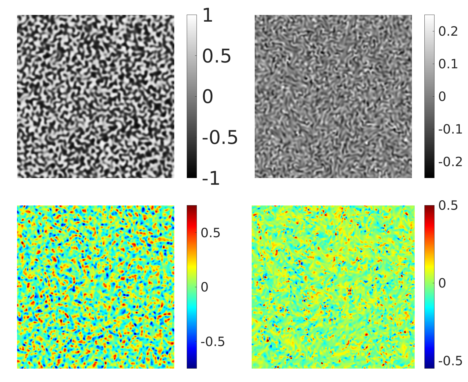
Figure 1: Pseudo-gray-scale plots of the $\phi$ field [at representative times in the nonequilibrium statistically steady state (NESS)] for the activity parameter (a) $|\zeta|=0.01$ and (b) $|\zeta|=1.5$. Pseudocolor plots of the vorticity field, normalized by the maximum of $|\omega|$, are shown in (c) and (d) for the parameters in (a) and (b), respectively.

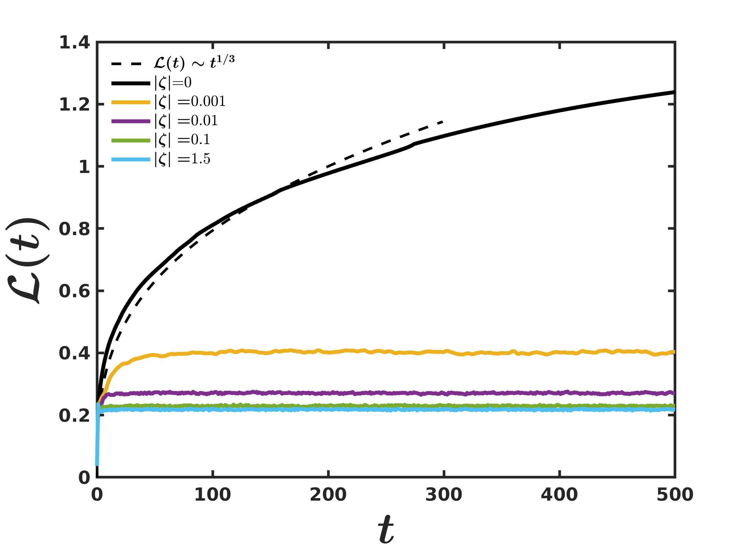
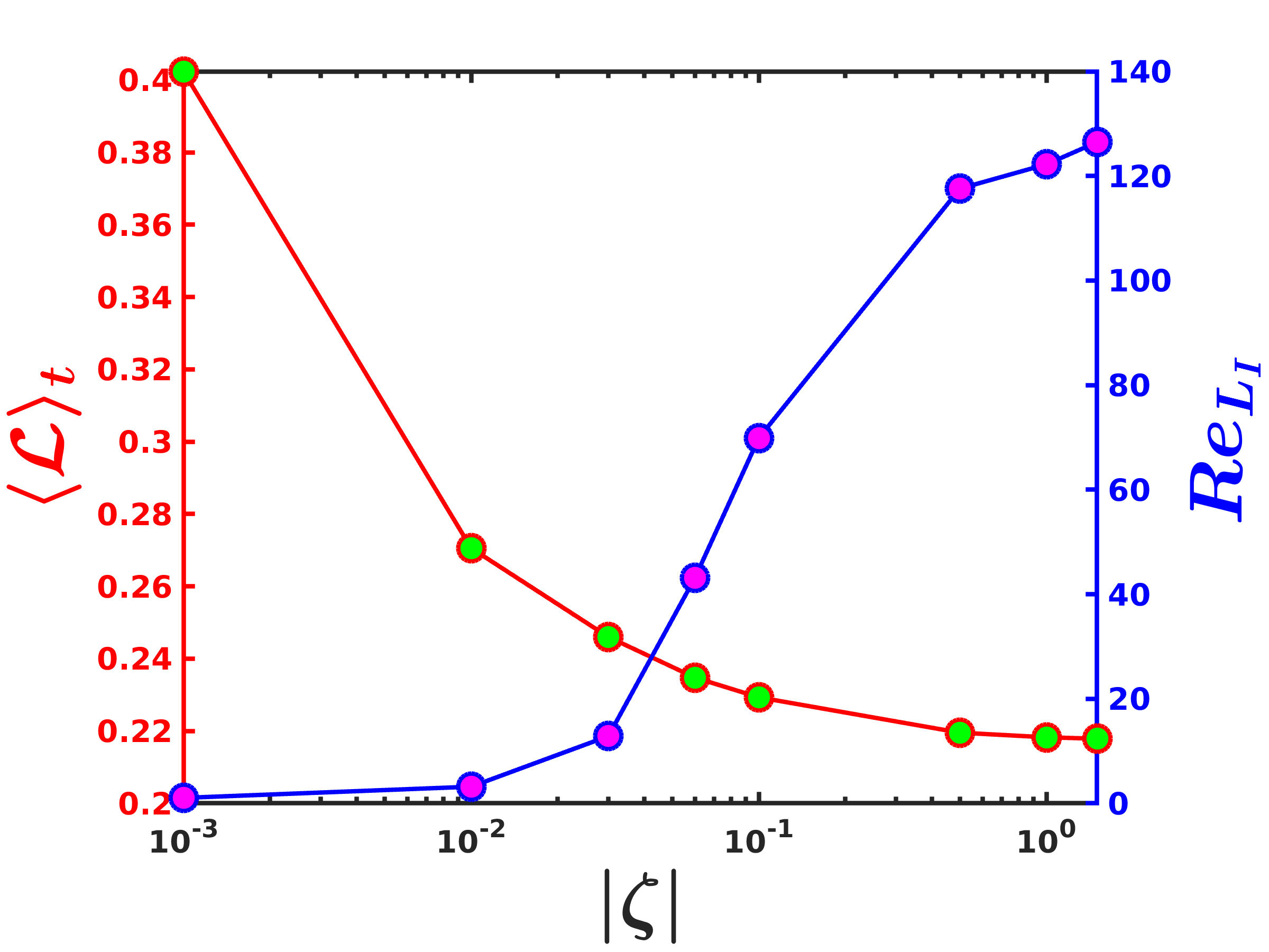
Figure 2: (a) Plot of the coarsening length scale $\mathcal{L}(t)$ [Eq. (8)] versus time $t$ for various values of $|\zeta|$; the plot for $\zeta=0$ shows growth that is consistent with the Lifshitz-Slyozov form $\mathcal{L}(t)\sim t^{1/3}$ (dashed line); $\mathcal{L}(t)$ saturates to a finite value for $|\zeta|>0$. (b) Log-linear plots of the mean coarsening-arrest scale $L_{c}=\langle\mathcal{L}(t)\rangle_{t}$ (red curve) and the integral-scale Reynolds number $Re_{L_{I}}$ (blue curve) versus $|\zeta|$.

II Model, Methods, and Statistical Measures

We introduce the active-CHNS model in Subsection II.1. In Subsection II.2 we describe the statistical measures we use to characterise active turbulence in this model. Finally, in Subsection II.3 we give the details of our pseudospectral DNS.

II.1 The Active Cahn-Hilliard-Navier-Stokes Model

We consider the incompressible active CHNS equations (also called active model H) to study active turbulence in systems of contractile swimmers [22, 24] in two spatial dimensions (2D):

$$\partial_{t}\phi+(\bm{u}\cdot\nabla)\phi = \text{M}\nabla^{2}\left(\frac{\delta\mathcal{F}}{\delta\phi}\right)\,;$$ (1)

$$\partial_{t}\omega+(\bm{u}\cdot\nabla)\omega = \nu\nabla^{2}\omega+\frac{3}{2}\epsilon\nabla\times(\nabla\cdot\bm{\Sigma}^{A})-\alpha\omega\,;\;$$ (2)

$$\nabla\cdot\bm{u} = 0\,;$$ (3)

$\omega$ is the vorticity field; $\nu$, $\alpha$, and M are the kinematic viscosity, bottom friction, and mobility, respectively. $\mathcal{F}$ is the Landau-Ginzburg variational free-energy functional

$$\mathcal{F}[\phi,\nabla\phi]=\int_{\Omega}\left[\frac{3}{16}\frac{\sigma}{\epsilon}(\phi^{2}-1)^{2}+\frac{3}{4}\sigma\epsilon|\nabla\phi|^{2}\right]\,,$$ (4)

in which the first term is a double-well potential with minima at $\phi=\pm 1$. The scalar order parameter $\phi$ is positive (negative) in regions where the microswimmer density is high (low); in the interfaces between these regions, $\phi$ varies smoothly, over a width $\epsilon$. The free-energy penalty for an interface is given by the bare surface tension $\sigma$. In the inherently nonequilibrium active model H all terms in the stress tensor do not follow from $\mathcal{F}$. In particular, we must include the stress tensor $\bm{\Sigma}^{A}$, which has the form of a nonlinear Burnett term and has the components [24, 22, 25, 29]

$$\Sigma^{A}_{ij}=-\zeta\left[\partial_{i}\phi\partial_{j}\phi-\frac{\delta_{ij}}{2}|\nabla\phi|^{2}\right]\,,$$ (5)

where $\zeta$, the activity coefficient, can take both positive and negative values: $\zeta<0$ ($\zeta>0$) for contractile (extensile) swimmers [22].

II.2 Statistical Characterisation

To characterise the statistical properties of active-scalar turbulence, we employ energy spectra and fluxes, which are familiar from classical fluid turbulence, and the spectrum of $\phi$. These quantities not only help us to understand, via DNS, the emergent turbulent like behaviour (characterized by spatiotemporal fluctuations) in Eqs. (1-3), but they also aid us in differentiating active scalar turbulence from classical 2D incompressible fluid turbulence [see, e.g., Refs. [30, 31, 32, 33]] and also turbulent patterns found in other active systems [see, e.g., Refs. [17, 18, 19, 20]]. We define the shell-averaged energy and phase-field spectra, respectively, both at time $t$ and averaged over time [the time average is denoted by $\langle\cdot\rangle_{t}$]:

$$\mathcal{E}(k,t) \equiv \sum_{k\leq k^{\prime}<k+1}|\hat{\bm{u}}(\bm{k}^{\prime},t)|^{2}\,;~{}~{}~{}\Phi(k,t)\equiv\sum_{k\leq k^{\prime}<k+1}|\hat{\phi}(\bm{k}^{\prime},t)|^{2}\,;$$

$$\mathcal{E}(k) \equiv \langle\mathcal{E}(k,t)\rangle_{t}\,;~{}~{}~{}\Phi(k)\equiv\langle\Phi(k,t)\rangle_{t}\,;$$ (6)

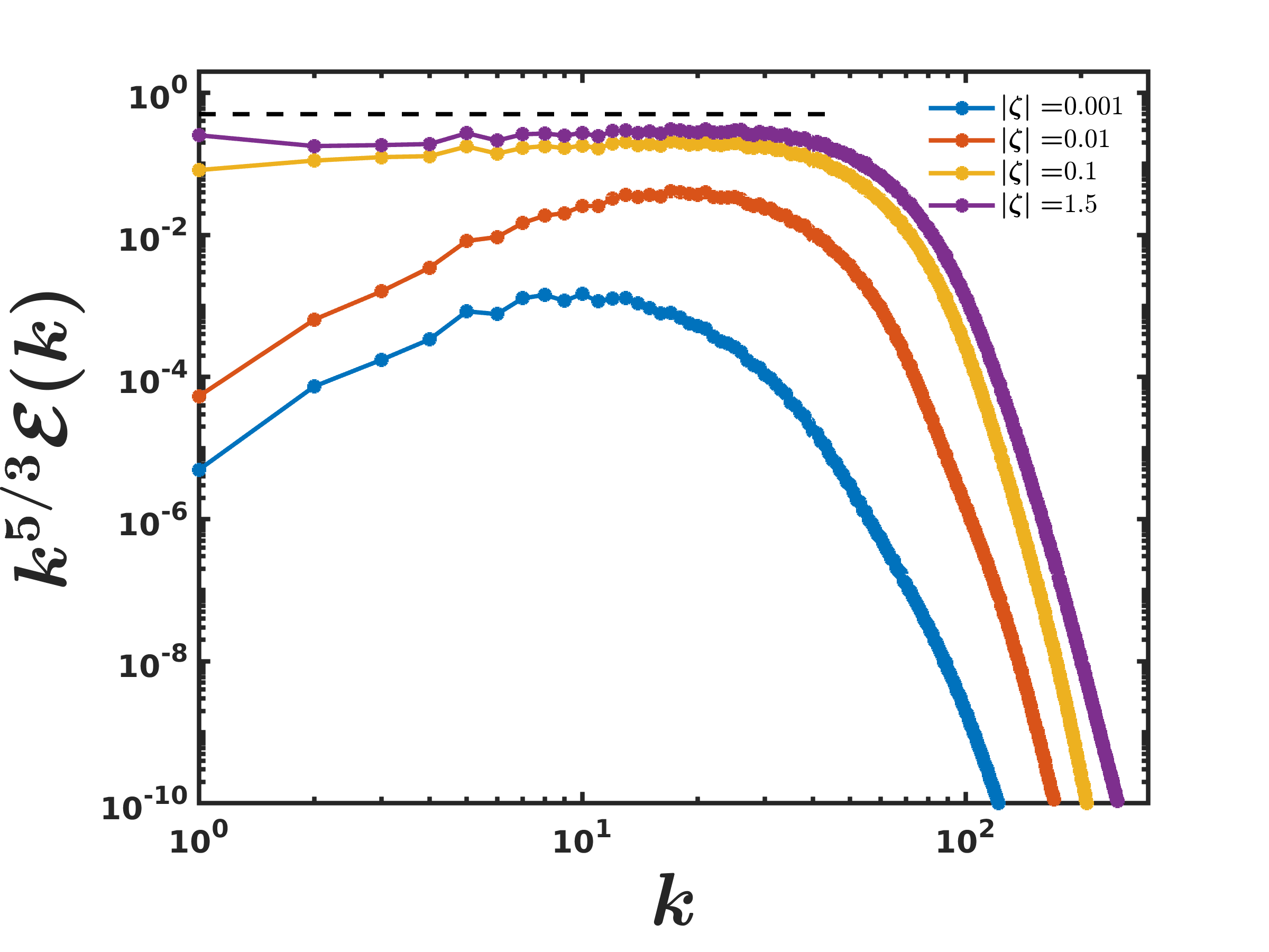
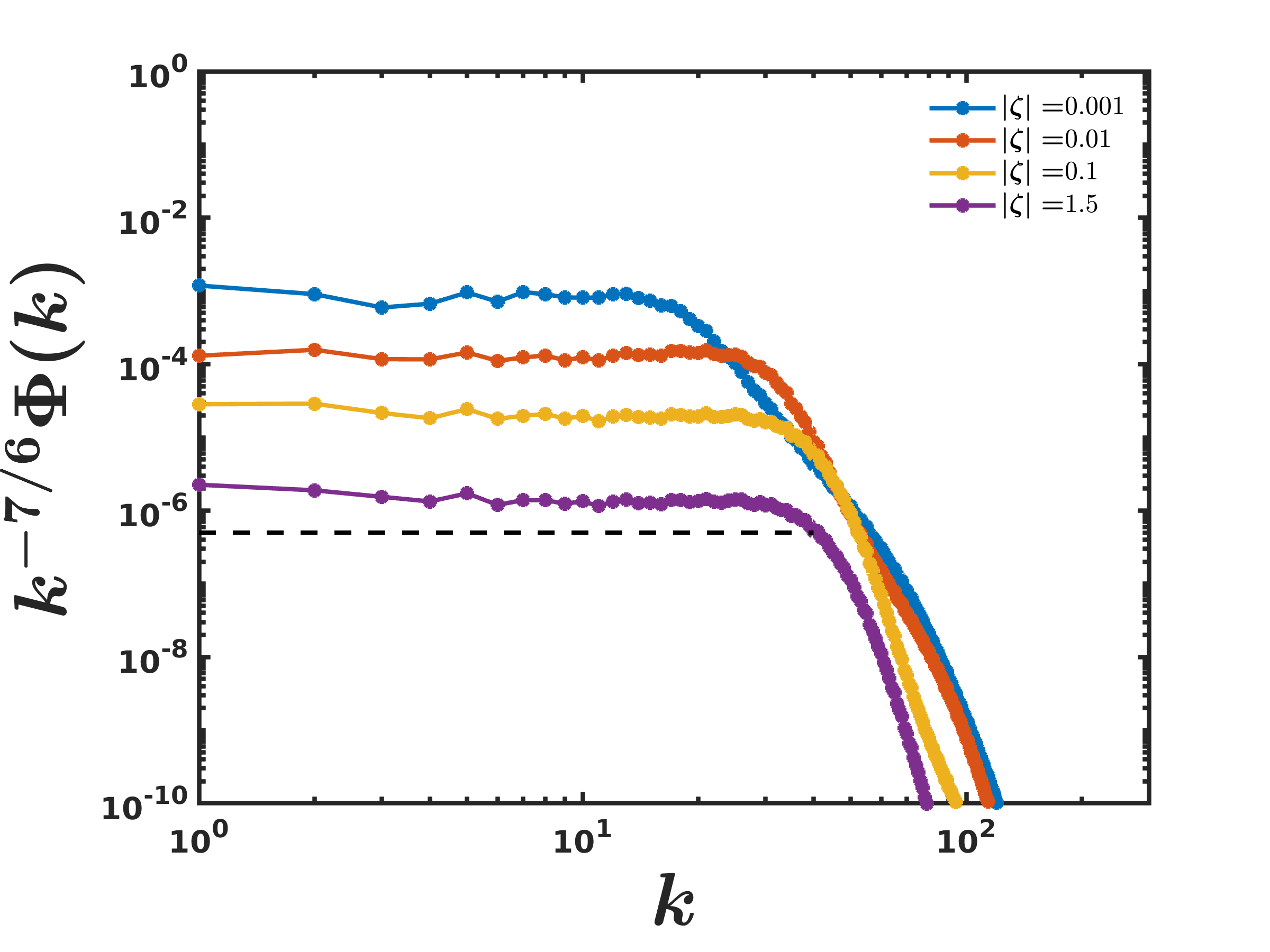
Figure 3: Log-log plots versus the wavenumber $k$ of spectra for $|\zeta|=0.001,0.01,0.1,1.5$: (a) The compensated energy spectrum $k^{5/3}\mathcal{E}(k)$. For $|\zeta|=0.1,1.5$, the exponent is $-5/3$ (black dotted line in the compensated spectrum). (b) The compensated phase-field spectrum $k^{-7/6}\Phi(k)$ for $|\zeta|=0.001,0.01,0.1,1.5$. These spectra show the power-law behaviour $\Phi(k)\sim k^{7/6}$ (black dotted line in the compensated spectrum).

the caret denotes a spatial Fourier transform. Our CHNS study of active scalar turbulence uses the Reynolds, Péclet, Weber, and the non-dimensional friction numbers that are, respectively:

Re $$= \frac{\text{L}_{I}u_{rms}}{\nu}\,;\;\;Pe=\frac{\epsilon{L}_{I}u_{rms}}{M\sigma}\,;$$

$$We = \frac{L_{I}u_{rms}^{2}}{\sigma}\,;\;\;\alpha^{\prime}=\frac{\alpha L_{I}}{u_{rms}}\,;$$ (7)

$u_{rms}$ and $L_{I}$ are, respectively, the root-mean-squared velocity and the fluid integral length scale; and $\mathcal{L}(t)$ and $L_{c}$ are the time-dependent and mean coarsening length scales; these are defined as follows:

$$u_{rms} = \left[\sum_{k}\mathcal{E}(k)\right]^{1/2}\;;\;\;\;L_{I}=2\pi\frac{\sum_{k}\mathcal{E}(k)}{\sum_{k}k\mathcal{E}(k)}\;;$$

$$\mathcal{L}(t) = \frac{\sum_{k}\Phi(k,t)}{\sum_{k}k\Phi(k,t)}\;;\;\;\;L_{c}=\langle\mathcal{L}(t)\rangle_{t}\;.$$ (8)

In Table 1, we provide the non-dimensional parameters from our direct numerical simulations (DNSs) for various values of the activity parameter $|\zeta|$. Furthermore, $\mathcal{E}(k,t)$ satisfies the following energy-budget equation [28, 34, 35]:

$$\partial_{t}\mathcal{E}(k,t)=T(k,t)+D_{\alpha}(k,t)+D_{\nu}(k,t)+S^{\phi}(k,t)\,,$$ (9)

where

$$T(k,t) = -\Re\left[\sum_{k\leq|\bm{k}^{\prime}|<k+1}[\hat{\bm{u}}(-\bm{k}^{\prime},t)\cdot\bm{P}(\bm{k}^{\prime})\cdot\widehat{(\bm{u}\cdot\nabla\bm{u})}(\bm{k}^{\prime},t)]\right],$$

$$D_{\alpha}(k,t) = -2\alpha\mathcal{E}(k,t),~{}~{}~{}~{}D_{\nu}(k,t)=-2\nu k^{2}\mathcal{E}(k,t),$$

$$S^{\phi}(k,t) = \Re\left[\sum_{k\leq|\bm{k}^{\prime}|<k+1}[\hat{\bm{u}}(-\bm{k}^{\prime},t)\cdot\bm{P}(\bm{k}^{\prime})\cdot\widehat{(\nabla\cdot\bm{\Sigma}^{A})}(\bm{k}^{\prime},t)]\right]$$ (10)

are, respectively, the energy transfer because of the inertial term, the energy dissipations arising from friction and the viscosity, and the energy transfer via the active-stress term; the transverse projector $\bm{P}(\bm{k})$, which enforces the incompressibility condition, has the components $P_{ij}\equiv(\delta_{ij}-{k_{i}k_{j}}/{k^{2}})$ . We also use the following mean energy transfers from the inertial, friction, viscous, and active-stress terms, and the associated kinetic-energy and active-stress fluxes [35]:

$$T(k) = \langle T(k,t)\rangle_{t}\,;\;\;\;\;S^{\phi}(k)=\langle S^{\phi}(k,t)\rangle_{t}\,;\;\;\;$$

$$D_{\alpha}(k) = \langle D_{\alpha}(k,t)\rangle_{t}\,;\;\;\;\;D_{\nu}(k)=\langle D_{\nu}(k,t)\rangle_{t}\,;$$

$$\Pi(k) = -\int_{0}^{k^{\prime}}T(k^{\prime})dk^{\prime}\,;\;\;\;\;\Pi^{\phi}(k)=-\int_{0}^{k^{\prime}}S^{\phi}(k^{\prime})dk^{\prime}\,.$$ (11)

II.3 Direct Numerical Simulation

We carry out DNSs of the active-CHNS partial differential equations (1)-(5) by using the pseudospectral method [36, 27, 37, 24] in a 2D periodic square domain, $\mathcal{D}\equiv[0,L]^{2}$, with $L$ the length of the side of the square. We evaluate spatial derivatives in Fourier space and the nonlinear terms in physical space. For time integration, we use the semi-implicit exponential-time-difference Runge-Kutta2 (ETDRK2) method [38]. We employ the $1/2$-dealiasing scheme to remove the Fourier aliasing errors [36, 27, 37, 24]. To resolve the interface of width $\epsilon$, we ensure that there are three grid points across the interface. We use a CUDA-C code that we have developed and optimised for an NVIDIA A100 processor.

II.4 Initial conditions

We use the following initial conditions for the $\omega$ and $\phi$ fields:

$$\omega(x,y,0)=0\,;~{}~{}~{}~{}\phi(x,y,0)=\phi_{0}+\xi(x,y)\,;$$ (12)

$\xi(x,y)$, a random number distributed uniformly on the interval $[-0.1,0.1]$, provides a random perturbation to the $\phi=\phi_{0}=0$ state.

III Results

In this Section we present a series of DNSs that we have designed to demonstrate how the activity of contractile swimmers [$\zeta<0$ in Eq. (5)] leads to active turbulence that is strong enough to suppress motility-induced phase separation. Our results are the active-turbulence counterparts of the suppression of phase separation (also called coarsening arrest) by fluid turbulence [see, e.g., Refs. [26, 27]].

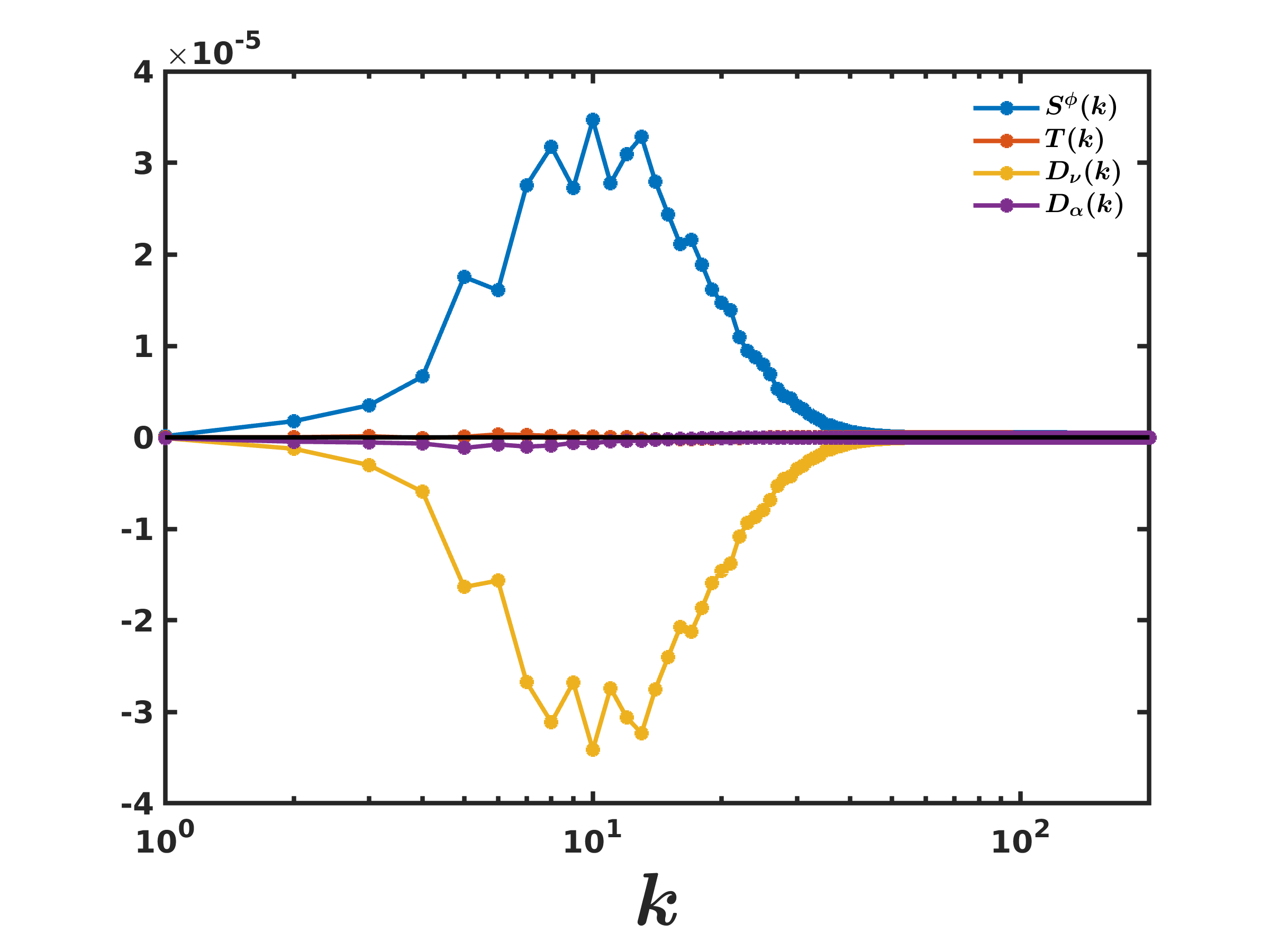
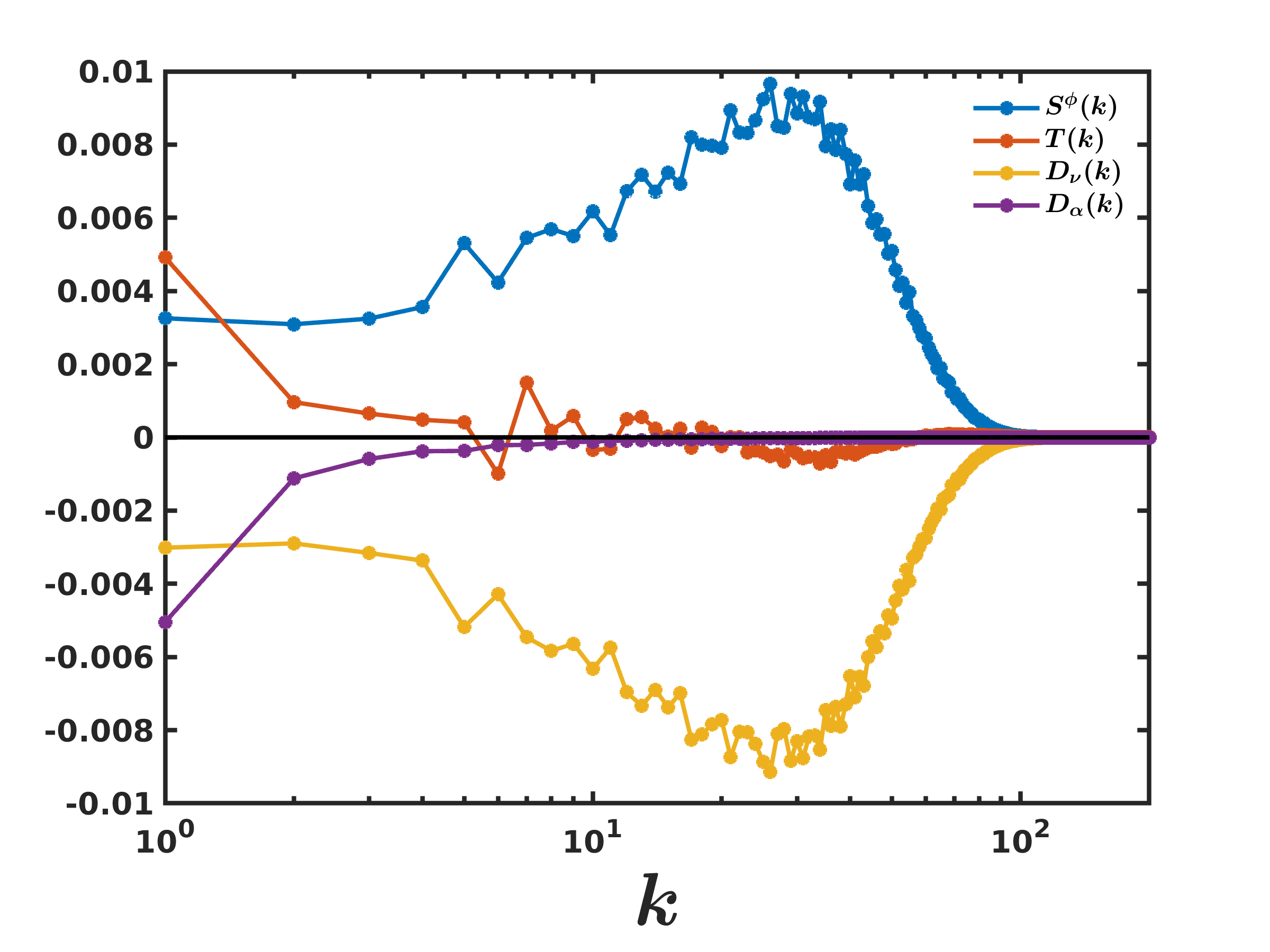
Figure 4: Plots versus $k$ (log scale) of the contributions $T(k),\;D_{\alpha}(k),\;D_{\nu}(k),\;\rm{and}\;S^{\phi}(k)$, in red, purple, yellow, and blue, respectively, for (a) $|\zeta|=0.001$ and (b) $|\zeta|=1.5$.

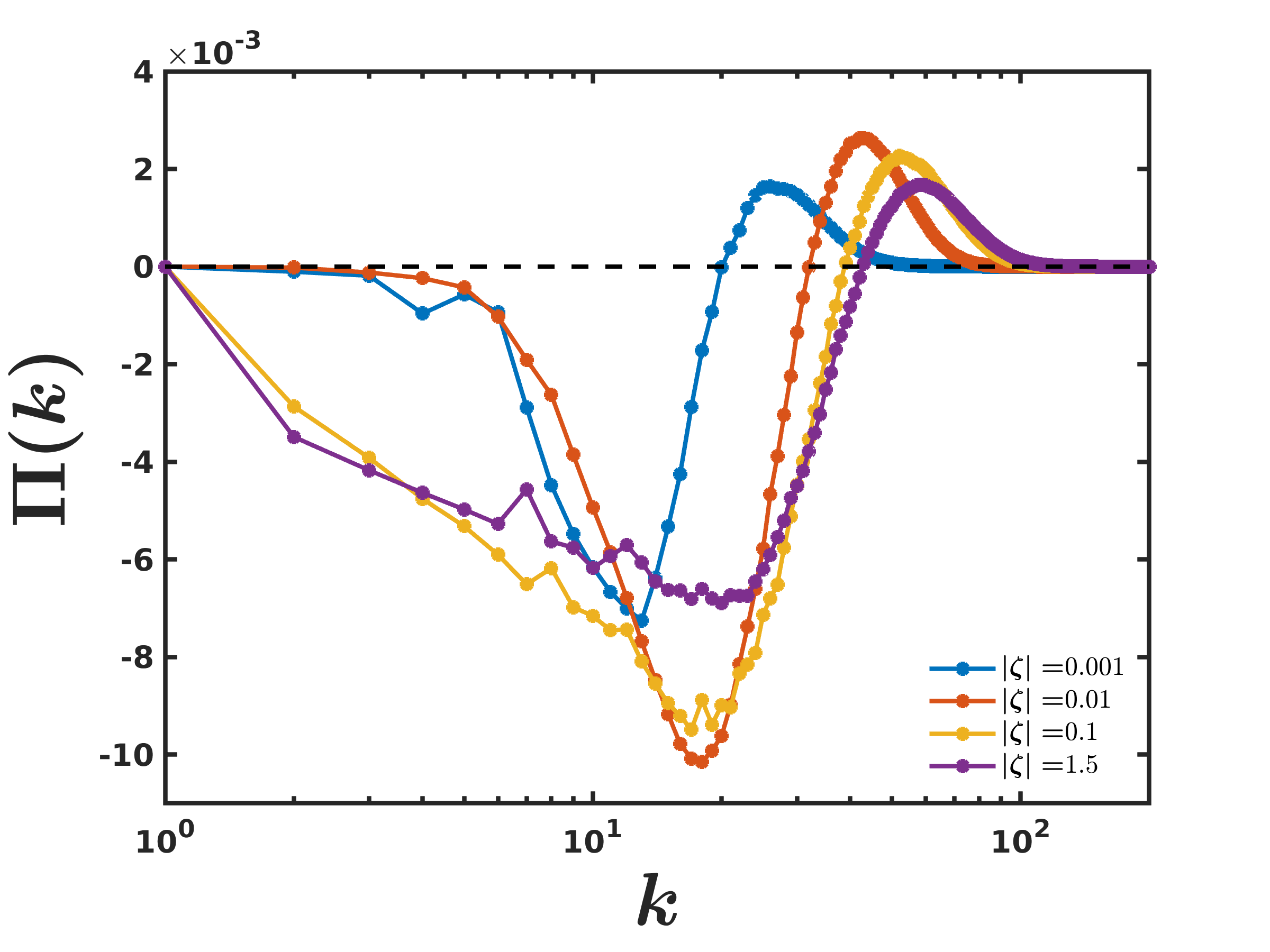
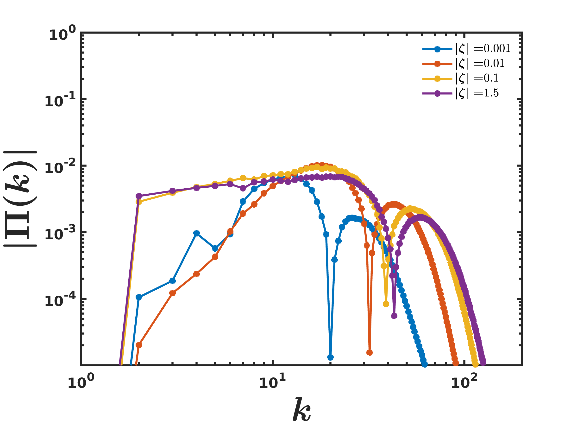
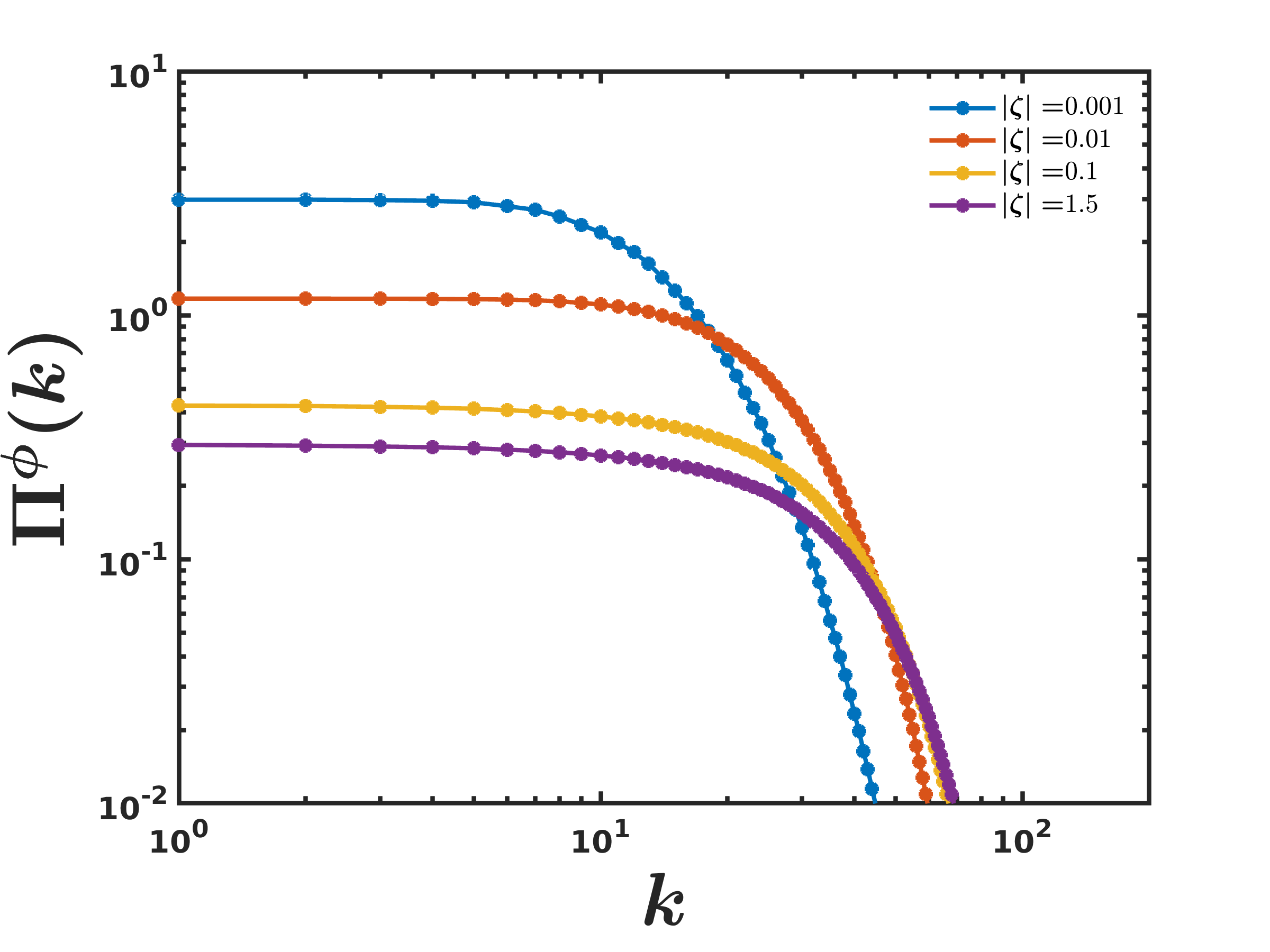
Figure 5: Plots for $|\zeta|=0.001,0.01,0.1,$ and $1.5$ of the normalized (a) energy flux $\Pi(k)L_{I}/u^{3}_{rms}$ versus $k$ (log scale) and log-log plots versus $k$ of (b) $|\Pi(k)|L_{I}/u^{3}_{rms}$ and (c) $\Pi^{\phi}(k)L_{I}/u^{3}_{rms}$.

We note that, if the activity $\zeta=0$, the stress tensor (5) vanishes, so the coupled Eqs. (1)-(5) decouple into Cahn-Hilliard equations or model B [39, 40] and the Navier Stokes equations [41, 42, 43] for a Newtonian fluid; the advection term for the $\phi$ field is set to zero by virtue of the initial conditions. Therefore, the domain growth or coarsening takes place solely via diffusion, without hydrodynamical effects, and it follows the well-established Lifshitz-Slyozov domain-growth form $\mathcal{L}(t)\sim t^{1/3}$ [see, e.g., Refs. [44, 40, 45]]; complete phase separation also occurs for extensile swimmers [22] that lead to $\zeta>0$.

We concentrate on active-turbulence-induced suppression of phase separation and the diffusive Lifshitz-Slyozov coarsening in our model (1)-(5) with contractile swimmers, for which the activity parameter $\zeta<0$ . Active turbulence and coarsening arrest in the active-CHNS model (1)-(5) can be visualized qualitatively by using pseudo-gray-scale plots of the $\phi$ field as we show in Figs. 1 (a) and (b) for $|\zeta|=0.01$ and (b) $|\zeta|=1.5$, respectively, at representative times in the nonequilibrium statistically steady state (NESS). In Figs. 1 (c) and (d), we present pseudocolor plots of the vorticity field, normalized by the maximum of $|\omega|$, for the parameters in Figs. 1 (a) and (b), respectively. These plots show clearly that the typical size of a single-phase domain decreases as activity-induced turbulence is enhanced by an increase in the value of $|\zeta|$.

We quantify active-turbulence-induced suppression of phase separation by plotting the coarsening length scale $\mathcal{L}(t)$ versus time $t$ in Fig. 2(a) for various values of $|\zeta|$; the plot for $\zeta=0$ shows growth that is consistent with the Lifshitz-Slyozov form $\mathcal{L}(t)\sim t^{1/3}$ (dashed line ). As $t$ increases, $\mathcal{L}(t)$ saturates to a finite value for $|\zeta|>0$, i.e., Eqs. (1)-(5) lead to coarsening-arrest because of active turbulence. In Fig. 2(b) we show how the mean coarsening-arrest scale $L_{c}=\langle\mathcal{L}(t)\rangle_{t}$ decreases as $|\zeta|$ increases (red curve); the attendant growth of the integral-scale Reynolds number $Re_{L_{I}}$ (blue curve) signals the enhancement of activity-induced turbulence.

We now characterise the statistical properties of activity-induced turbulence in Eqs. (1)-(5). We begin with log-log plots of compensated energy and scalar-$\phi$ spectra, $k^{5/3}\mathcal{E}(k)$ and $k^{-7/6}\Phi(k)$, versus $k$, in Figs. 3 (a) and (b), respectively, for various values of $|\zeta|$. These plots suggest that, as $\zeta$ increases, the activity-induced turbulence in this systems leads to a nonequilibrium statistically steady state (NESS) with an inertial range of scales in which the energy spectrum has a power-law form that is consistent with $\mathcal{E}(k)\sim k^{-5/3}$. We show below that this power-law spectrum arises because of an inverse cascade of energy. Its power-law form can then be surmised as in statistically steady homogeneous and isotropic 2D-fluid turbulence with an inverse energy cascade [30, 31, 32, 33]. Note that this power-law region extends over nearly one-and-a-half decades of $k$ at the largest value $|\zeta|(=1.5)$ that we consider.

Run	$|\zeta|$	$Re_{L_{I}}$	$\alpha^{\prime}$	$Pe$	$We$
R1	0	0	$-$	0	0
R2	0.001	$1.1\times 10^{0}$	$5.6\times 10^{-2}$	$2.8\times 10^{-1}$	$1.6\times 10^{-4}$
R3	0.01	$3.2\times 10^{0}$	$7.9\times 10^{-3}$	$8.5\times 10^{-1}$	$2.3\times 10^{-3}$
R4	0.03	$1.3\times 10^{1}$	$6.6\times 10^{-3}$	$3.5\times 10^{0}$	$2\times 10^{-2}$
R5	0.05	$4.3\times 10^{1}$	$7.8\times 10^{-3}$	$1.2\times 10^{1}$	$1.1\times 10^{-1}$
R6	0.1	$6.9\times 10^{1}$	$7.0\times 10^{-3}$	$1.9\times 10^{1}$	$2.3\times 10^{-1}$
R7	0.5	$1.1\times 10^{2}$	$5.8\times 10^{-3}$	$3.2\times 10^{1}$	$5.3\times 10^{-1}$
R8	1	$1.2\times 10^{2}$	$6.8\times 10^{-3}$	$3.3\times 10^{1}$	$5.8\times 10^{-1}$
R9	1.5	$1.3\times 10^{2}$	$5.7\times 10^{-3}$	$3.4\times 10^{1}$	$6.1\times 10^{-1}$

Table 1: The values of various parameters in our DNS runs R1-R9. The following parameters are fixed in all these runs: $N=1024,\;\text{grid size}\;\;dx=2\pi/N,\;\epsilon=3dx,\;L=2\pi,\;\text{Cn}=3dx/L,\;M=\epsilon^{2}/2,\;\sigma=1,\;\nu=5\times 10^{-3}$, $\alpha=0.01$.

We examine the energy-transfer mechanisms in the NESS of activity-induced turbulence in Eqs. (1)-(5) by using the energy-budget equation (9) and evaluating the relevant scale-by-scale energy contributions [28, 34, 35]. In Figs. 4(a) and (b) we present, for the illustrative values $|\zeta|=0.001$ and (b) $|\zeta|=1.5$, respectively, plots versus $k$ (log scale) of the inertial, friction, viscous, and active-stress contributions $T(k)\;({\rm{red}}),\;D_{\alpha}(k)\;({\rm{purple}}),\;D_{\nu}(k)\;({\rm{yellow}})$ and $S^{\phi}(k)\;({\rm{blue}}),$ which we have defined in Eq. (11). Such plots indicate that, for low values of $|\zeta|$, the contributions of $T(k)$ and $D_{\alpha}(k)$ are negligible [Fig. 4(a)], so, in the NESS with $\langle\partial_{t}\mathcal{E}(k,t)\rangle_{t}=0$, dominant balance yields $D_{\nu}(k)+S^{\phi}(k)=0$. As $|\zeta|$ increases, both $T(k)$ and $D_{\alpha}(k)$ increase in magnitude [Fig. 4(b)], so a four-term balance is required in the NESS.

To show that activity-induced turbulence exhibits a bona fide inertial range we present plots for $|\zeta|=0.001,0.01,0.1,$ and $1.5$ of the energy flux $\Pi(k)$ [Eq. 11] versus $k$ (log scale) [Fig. 5(a)]. We also present log-log plots versus $k$ of $|\Pi(k)|$ [Fig. 5(b)] and $\Pi^{\phi}(k)$ [Fig. 5(c)]. These plots show constant fluxes over at least one decade of the wavenumber $k$, so we have a well-defined inertial range, that has a remarkable similarity with fluid turbulence [48]. The sign of $\Pi(k)$ in this range of scales indicates that activity-induced turbulence in Eqs. (1)-(5) yields an inverse cascade of energy that is reminiscent of a similar cascade in 2D statistically steady homogeneous and isotropic fluid turbulence [30, 31, 32, 33]. By comparing the different plots in Fig. 5(a), we see that this inverse cascade is suppressed as $|\zeta|$ decreases; this is reminiscent of similar cascade suppression in instability-driven 2D turbulence [49].

IV Conclusions

We have uncovered activity-induced homogeneous and isotropic turbulence in the active Cahn-Hilliard-Navier-Stokes equations (CHNS), which provides a natural theoretical framework for our study, in which a single scalar order parameter $\phi$ [positive (negative) in regions where the microswimmer density is high (low)] is coupled with the velocity field $\bm{u}$. The activity of the microswimmers is governed by an activity parameter $\zeta$ that is positive for extensile swimmers and negative for contractile swimmers [see Eqs. (1)-(5)]. With extensile swimmers, this system undergoes complete phase separation, as in binary-fluid mixtures [22]. By carrying out extensive pseudospectral direct numerical simulations (DNSs) we have shown that this model develops an emergent nonequilibrium, but statistically steady, state (NESS) of active turbulence, for the case of contractile swimmers, if $\zeta$ is sufficiently large and negative. This turbulence arrests the phase separation into regions with positive and negative values of $\phi$, as in conventional fluid turbulence leads to the suppression of phase separation in a binary-fluid mixture [26, 27, 28].

We have quantified this suppression by showing how the coarsening-arrest length $\mathcal{L}(t)$ scale does not grow indefinitely, with time $t$, but saturates at a finite value at large times. We have then characterised the statistical properties of this active-scalar turbulence by employing the energy spectrum $\mathcal{E}(k)$ and the fluxes $\Pi(k)$ and $\Pi^{\phi}(k)$. We have also obtained the spectrum of $\phi$, which is used in studies of phase separation. For sufficiently high Reynolds numbers, we have shown that the energy spectrum $\mathcal{E}(k)$ displays an inertial range, with a power-law dependence on the wavenumber $k$. We have demonstrated that, in this range, the flux $\Pi(k)$ assumes a nearly constant, negative value, which indicates that the system shows an inverse cascade of energy that is similar to its counterpart in 2D homogeneous and isotropic fluid turbulence, even though energy injection occurs over a wide range of wavenumbers in our active-CHNS model.

Our statistical characaterization of active-CHNS turbulence shows that it is fundamentally different from conventional 2D fluid turbulence [30, 31], forced 2D CHNS turbulence [27], and other types of active-fluid turbulence, discussed, e.g., in Refs. [1, 2, 3, 4, 5, 6, 7, 8, 9, 25, 10, 11]. For large values of $|\zeta|$, active-CHNS turbulence has some similarities with conventional 2D fluid turbulence and 2D forced CHNS turbulence, inasmuch as it shows an inverse-cascade region with $E(k)\sim k^{-5/3}$. The $|\zeta|$-dependent, small-$k$, power-law regime in $E(k)$ is qualitatively reminiscent of parameter-dependent small-$k$ power-law regimes in energy-spectra in some minimal models for bacterial turbulence [16, 3, 4, 7, 11, 8, 9]. The scalar spectrum $\Phi(k)$ of active-CHNS turbulence shows a substantial power-law regime which is different from that in conventional forced 2D CHNS turbulence [27]. The fluxes and energy budgets in active-CHNS turbulence are also markedly different from their counterparts in other types of 2D turbulence. Our study investigates the effects of active-CHNS turbulence that is distinct from the suppression of motility-induced phase separation in the active model H [22] with external noise.

We hope, therefore, that our active-CHNS study will lead to investigations of experimental realisations of this system. Our results are of potential relevance to systems of contractile swimmers, e.g., Chlamydomonas reinhardtii [50, 51] (C. reinhardtii) and synthetic active colloids  [52, 53]. We look forward to the experimental verification of our results, especially in the former system, where it should be possible to control the activity by changing the oxygen concentration in low-light conditions.

References

- Wensink et al. [2012] H. H. Wensink, J. Dunkel, S. Heidenreich, K. Drescher, R. E. Goldstein, H. Löwen, and J. M. Yeomans, Meso-scale turbulence in living fluids, Proceedings of the national academy of sciences 109, 14308 (2012).
- Qi et al. [2022] K. Qi, E. Westphal, G. Gompper, and R. G. Winkler, Emergence of active turbulence in microswimmer suspensions due to active hydrodynamic stress and volume exclusion, Communications Physics 5, 49 (2022).
- Alert et al. [2022] R. Alert, J. Casademunt, and J.-F. Joanny, Active turbulence, Annual Review of Condensed Matter Physics 13, 143 (2022).
- Mukherjee et al. [2023] S. Mukherjee, R. K. Singh, M. James, and S. S. Ray, Intermittency, fluctuations and maximal chaos in an emergent universal state of active turbulence, Nature Physics , 1 (2023).
- Dunkel et al. [2013a] J. Dunkel, S. Heidenreich, K. Drescher, H. H. Wensink, M. Bär, and R. E. Goldstein, Fluid dynamics of bacterial turbulence, Physical review letters 110, 228102 (2013a).
- Kaiser et al. [2014] A. Kaiser, A. Peshkov, A. Sokolov, B. Ten Hagen, H. Löwen, and I. S. Aranson, Transport powered by bacterial turbulence, Physical review letters 112, 158101 (2014).
- Joy et al. [2020] A. Joy et al., Friction scaling laws for transport in active turbulence, Physical Review Fluids 5, 024302 (2020).
- Linkmann et al. [2019] M. Linkmann, G. Boffetta, M. C. Marchetti, and B. Eckhardt, Phase transition to large scale coherent structures in two-dimensional active matter turbulence, Physical review letters 122, 214503 (2019).
- Linkmann et al. [2020] M. Linkmann, M. C. Marchetti, G. Boffetta, and B. Eckhardt, Condensate formation and multiscale dynamics in two-dimensional active suspensions, Physical Review E 101, 022609 (2020).
- Aranson [2022] I. S. Aranson, Bacterial active matter, Reports on Progress in Physics 85, 076601 (2022).
- Kiran et al. [2023] K. V. Kiran, A. Gupta, A. K. Verma, and R. Pandit, Irreversibility in bacterial turbulence: Insights from the mean-bacterial-velocity model, Physical Review Fluids 8, 023102 (2023).
- Opathalage et al. [2019] A. Opathalage, M. M. Norton, M. P. Juniper, B. Langeslay, S. A. Aghvami, S. Fraden, and Z. Dogic, Self-organized dynamics and the transition to turbulence of confined active nematics, Proceedings of the National Academy of Sciences 116, 4788 (2019).
- Wu et al. [2017] K.-T. Wu, J. B. Hishamunda, D. T. Chen, S. J. DeCamp, Y.-W. Chang, A. Fernández-Nieves, S. Fraden, and Z. Dogic, Transition from turbulent to coherent flows in confined three-dimensional active fluids, Science 355, eaal1979 (2017).
- Dunkel et al. [2013b] J. Dunkel, S. Heidenreich, M. Bär, and R. E. Goldstein, Minimal continuum theories of structure formation in dense active fluids, New Journal of Physics 15, 045016 (2013b).
- Alert et al. [2020] R. Alert, J.-F. Joanny, and J. Casademunt, Universal scaling of active nematic turbulence, Nature Physics 16, 682 (2020).
- Bratanov et al. [2015] V. Bratanov, F. Jenko, and E. Frey, New class of turbulence in active fluids, Proceedings of the National Academy of Sciences 112, 15048 (2015).
- Thampi et al. [2013] S. P. Thampi, R. Golestanian, and J. M. Yeomans, Velocity correlations in an active nematic, Physical review letters 111, 118101 (2013).
- Thampi et al. [2014] S. P. Thampi, R. Golestanian, and J. M. Yeomans, Vorticity, defects and correlations in active turbulence, Philosophical Transactions of the Royal Society A: Mathematical, Physical and Engineering Sciences 372, 20130366 (2014).
- Chatterjee et al. [2021] R. Chatterjee, N. Rana, R. A. Simha, P. Perlekar, and S. Ramaswamy, Inertia drives a flocking phase transition in viscous active fluids, Physical Review X 11, 031063 (2021).
- Rorai et al. [2022] C. Rorai, F. Toschi, and I. Pagonabarraga, Coexistence of active and hydrodynamic turbulence in two-dimensional active nematics, Physical Review Letters 129, 218001 (2022).
- Saha et al. [2020] S. Saha, J. Agudo-Canalejo, and R. Golestanian, Scalar active mixtures: The nonreciprocal cahn-hilliard model, Physical Review X 10, 041009 (2020).
- Tiribocchi et al. [2015] A. Tiribocchi, R. Wittkowski, D. Marenduzzo, and M. E. Cates, Active model h: scalar active matter in a momentum-conserving fluid, Physical review letters 115, 188302 (2015).
- Frohoff-Hülsmann et al. [2023] T. Frohoff-Hülsmann, U. Thiele, and L. M. Pismen, Non-reciprocity induces resonances in a two-field cahn–hilliard model, Philosophical Transactions of the Royal Society A 381, 20220087 (2023).
- Padhan and Pandit [2023] N. B. Padhan and R. Pandit, Activity-induced droplet propulsion and multifractality, Physical Review Research 5, L032013 (2023).
- Bhattacharjee and Kirkpatrick [2022] J. Bhattacharjee and T. Kirkpatrick, Activity induced turbulence in driven active matter, Physical Review Fluids 7, 034602 (2022).
- Perlekar et al. [2014] P. Perlekar, R. Benzi, H. J. Clercx, D. R. Nelson, and F. Toschi, Spinodal decomposition in homogeneous and isotropic turbulence, Physical review letters 112, 014502 (2014).
- Perlekar et al. [2017] P. Perlekar, N. Pal, and R. Pandit, Two-dimensional turbulence in symmetric binary-fluid mixtures: Coarsening arrest by the inverse cascade, Scientific Reports 7, 44589 (2017).
- Perlekar [2019] P. Perlekar, Kinetic energy spectra and flux in turbulent phase-separating symmetric binary-fluid mixtures, Journal of Fluid Mechanics 873, 459 (2019).
- Das et al. [2020] A. Das, J. Bhattacharjee, and T. Kirkpatrick, Transition to turbulence in driven active matter, Physical Review E 101, 023103 (2020).
- Boffetta and Ecke [2012] G. Boffetta and R. E. Ecke, Two-dimensional turbulence, Annual review of fluid mechanics 44, 427 (2012).
- Pandit et al. [2017] R. Pandit, D. Banerjee, A. Bhatnagar, M. Brachet, A. Gupta, D. Mitra, N. Pal, P. Perlekar, S. S. Ray, V. Shukla, and D. Vincenzi, An overview of the statistical properties of two-dimensional turbulence in fluids with particles, conducting fluids, fluids with polymer additives, binary-fluid mixtures, and superfluids, Physics of Fluids 29, 111112 (2017), https://pubs.aip.org/aip/pof/article-pdf/doi/10.1063/1.4986802/15675695/111112_1_online.pdf .
- Kraichnan [1967] R. H. Kraichnan, Inertial ranges in two-dimensional turbulence, The Physics of Fluids 10, 1417 (1967).
- Kraichnan and Montgomery [1980] R. H. Kraichnan and D. Montgomery, Two-dimensional turbulence, Reports on Progress in Physics 43, 547 (1980).
- Alexakis and Biferale [2018] A. Alexakis and L. Biferale, Cascades and transitions in turbulent flows, Physics Reports 767, 1 (2018).
- Verma [2019] M. K. Verma, Energy transfers in fluid flows: multiscale and spectral perspectives (Cambridge University Press, 2019).
- Canuto et al. [2012] C. Canuto, M. Y. Hussaini, A. Quarteroni, A. Thomas Jr, et al., Spectral methods in fluid dynamics (Springer Science Business Media, 2012).
- Pal et al. [2016] N. Pal, P. Perlekar, A. Gupta, and R. Pandit, Binary-fluid turbulence: Signatures of multifractal droplet dynamics and dissipation reduction, Phys. Rev. E 93, 063115 (2016).
- Cox and Matthews [2002] S. M. Cox and P. C. Matthews, Exponential time differencing for stiff systems, Journal of Computational Physics 176, 430 (2002).
- Hohenberg and Halperin [1977] P. C. Hohenberg and B. I. Halperin, Theory of dynamic critical phenomena, Reviews of Modern Physics 49, 435 (1977).
- Puri [2009] S. Puri, Kinetics of phase transitions, in Kinetics of phase transitions (CRC press, 2009) pp. 13–74.
- Navier [1823] C. Navier, Mémoire sur les lois du mouvement des fluides, Mémoires de l’Académie Royale des Sciences de l’Institut de France 6, 389 (1823).
- Stokes [1901] G. G. Stokes, Mathematical and physical papers, Vol. 3 (1901).
- Doering and Gibbon [1995] C. R. Doering and J. D. Gibbon, Applied analysis of the Navier-Stokes equations, 12 (Cambridge university press, 1995).
- Lifshitz and Slyozov [1961] I. M. Lifshitz and V. V. Slyozov, The kinetics of precipitation from supersaturated solid solutions, Journal of physics and chemistry of solids 19, 35 (1961).
- Bray [2002] A. J. Bray, Theory of phase-ordering kinetics, Advances in Physics 51, 481 (2002).
- Note [1] At low inertia motility-induced phase separation is also suppressed in this model [22].
- Note [2] In any DNS in a finite domain, approaches a finite value that is comparable to the linear size of the domain.
- Frisch [1995] U. Frisch, Turbulence: the legacy of AN Kolmogorov (Cambridge university press, 1995).
- van Kan et al. [2022] A. van Kan, B. Favier, K. Julien, and E. Knobloch, Spontaneous suppression of inverse energy cascade in instability-driven 2-d turbulence, Journal of Fluid Mechanics 952, R4 (2022).
- Yeomans et al. [2014] J. M. Yeomans, D. O. Pushkin, and H. Shum, An introduction to the hydrodynamics of swimming microorganisms, The European Physical Journal Special Topics 223, 1771 (2014).
- Fragkopoulos et al. [2021] A. A. Fragkopoulos, J. Vachier, J. Frey, F.-M. Le Menn, M. G. Mazza, M. Wilczek, D. Zwicker, and O. Baumchen, Self-generated oxygen gradients control collective aggregation of photosynthetic microbes, Journal of the Royal Society Interface 18, 20210553 (2021).
- Zöttl and Stark [2016] A. Zöttl and H. Stark, Emergent behavior in active colloids, Journal of Physics: Condensed Matter 28, 253001 (2016).
- Howse et al. [2007] J. R. Howse, R. A. Jones, A. J. Ryan, T. Gough, R. Vafabakhsh, and R. Golestanian, Self-motile colloidal particles: from directed propulsion to random walk, Physical review letters 99, 048102 (2007).