Credal Learning Theory

Abstract

Statistical learning theory is the foundation of machine learning, providing theoretical bounds for the risk of models learnt from a (single) training set, assumed to issue from an unknown probability distribution. In actual deployment, however, the data distribution may (and often does) vary, causing domain adaptation/generalization issues. In this paper we lay the foundations for a ‘credal’ theory of learning, using convex sets of probabilities (credal sets) to model the variability in the data-generating distribution. Such credal sets, we argue, may be inferred from a finite sample of training sets. Bounds are derived for the case of finite hypotheses spaces (both assuming realizability or not) as well as infinite model spaces, which directly generalize classical results.

1 Introduction

Statistical Learning Theory (SLT) considers the problem of predicting an output $y\in\mathcal{Y}$ given an input $x\in\mathcal{X}$ by means of a mapping $h:\mathcal{X}\rightarrow\mathcal{Y}$, $h\in\mathcal{H}$, called model or hypothesis, belonging to model (or hypotheses) space $\mathcal{H}$. The loss function $l:(\mathcal{X}\times\mathcal{Y})\times\mathcal{H}\rightarrow\mathbb{R}$ measures the error committed by a model $h\in\mathcal{H}$. For instance, the zero-one loss is defined as $l((x,y),h)\doteq\mathbbm{I}[y\neq h(x)]$, where $\mathbbm{I}$ denotes the indicator function. This function assigns a zero value to correct predictions and one to incorrect ones. Input-output pairs are usually assumed to be generated i.i.d. by a probability distribution $P^{\star}$, which is unknown. The expected risk – or expected loss – of the model $h$,

$$L(h)\equiv L_{P^{\star}}(h) \doteq\mathbb{E}_{P^{\star}}[l((x,y),h)]$$

$$=\int_{\mathcal{X}\times\mathcal{Y}}l((x,y),h)P^{\star}(\text{d}(x,y)),$$

measures the expected value – taken with respect to $P^{\star}$ – of loss $l$. The expected risk minimizer

$$h^{\star}\in\operatorname*{arg\,min}_{h\in\mathcal{H}}L(h),$$

is any hypothesis in the given model space $\mathcal{H}$ that minimizes the expected risk. Given a training dataset $D=\{(x_{1},y_{1}),\ldots,(x_{n},y_{n})\}$ whose elements are drawn i.i.d. from probability distribution $P^{\star}$, the empirical risk of a hypothesis $h$ is the average loss over $D$. The empirical risk minimizer (ERM), i.e., the model $\hat{h}$ one actually learns from the training set $D$, is the one minimizing the empirical risk.
Statistical Learning Theory seeks upper bounds on the expected risk $L(\hat{h})$ of the ERM $\hat{h}$, and in turn, on the excess risk, that is, on the difference between $L(\hat{h})$, and the lowest expected risk $L(h^{\star})$. This endeavor is pursued under increasingly more relaxed assumptions about the nature of the hypotheses space $\mathcal{H}$. Two common such assumptions are that either the model space is finite, or that there exists a model with zero expected risk (realizability).

In real-world situations, however, the data distribution may (and often does) vary, causing issues of domain adaptation (DA) or generalization (DG). Domain adaptation and generalization are interrelated yet distinctive concepts in machine learning, as they both deal with the challenges of transferring knowledge across different domains. The main goal of DA is to adapt a machine learning model trained on source domains to perform well on target domains. In opposition, DG aims to train a model that can generalize well to unseen data/domains not available during training. In simple terms, DA works on the assumption that our source and target domains are related to each other, meaning that they somehow follow a similar data-generating probability distribution. DG, instead, assumes that the trained model should be able to handle unseen target data (Piva et al., 2023).

Some attempts to derive generalization bounds under more realistic conditions within classical SLT have been made. However, those approaches are characterized by a lack of generalizability, and the use of strong assumptions. A more detailed account of the state of the art and their limitations is discussed Section 2.

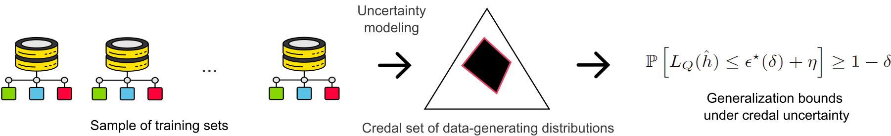
Figure 1: Graphical representation of the proposed learning framework. Given an available finite sample of training sets, each assumed to be generated by a single data distribution, one can learn a credal set $\mathcal{P}$ of data distributions in either a frequentist or subjectivist fashion (Section 3). This allows us to derive generalization bounds under credal uncertainty (Section 4).

Imprecise Probabilities (IPs) can provide a radically different solution to the construction of bounds in learning theory. A hierarchy of formalisms aimed at mathematically modeling the ‘epistemic’ uncertainty induced by sources such as lack of data, missing data or data which is imprecise in nature (Cuzzolin, 2020; Sale et al., 2023a, b), IPs have been successfully employed in the design of neural networks providing both better accuracy and uncertainty quantification to predictions (Sensoy et al., 2018; Manchingal and Cuzzolin, 2022; Manchingal et al., 2023; Caprio et al., 2023a; Lu et al., 2024; Wang et al., 2024). To date, however, they have never been considered as a tool to address the foundational issues of statistical learning theory associated with data drifting.

1.1 Contributions

This paper provides two innovative contributions: (1) the formal definition of a new learning setting in which models are inferred from a (finite) sample of training sets, rather than a single training set, each assumed to have been generated by a single data distribution (as in classical SLT); (2) the derivation of generalization bounds to the expected risk of a model learnt in this new learning setting, under the assumption that the epistemic uncertainty induced by the available training sets can be described by a credal set, i.e., a convex set of (data-generating) probability distributions.

The overall framework is illustrated in Fig. 1.

Generalized upper bounds under credal uncertainty are derived under three increasingly realistic sets of assumptions, mirroring classical statistical learning theory treatment: (i) finite hypotheses spaces with realizability, (ii) finite hypotheses spaces without realizability, and (iii) infinite hypotheses spaces. We show that the corresponding classical results in SLT are special cases of the ones derived in the present paper.

1.2 Structure of the paper

The paper is structured as follows. First (Section 2) we present the existing work in addressing data distribution shifts in learning theory. We then introduce our new learning framework (Section 3). In Section 4 we illustrate the bounds derived under credal uncertainty, and show how classical results can be recovered as special cases. Section 5 concludes and outlines future undertakings.

2 Related Work

The standard statistical approach is based on the assumption that test and training data are independent and identically distributed (i.i.d.) according to an unknown distribution. This assumption can fall short in real-world applications: as a result, many recent papers have been focusing on the “Out of Distribution” (OOD) generalization problem, also known as domain generalization (DG), to address the discrepancy between test and training distribution(s) (Gulrajani and Lopez-Paz, 2020; Koh et al., 2021). An extensive surveys of existing methods and approaches to DG can be found in Zhou et al. (2022); Wang et al. (2022).

Although several proposals for learning bounds with theoretical guarantees have been made within domain adaptation (DA), only a few attempts have been made in the field of DG (Redko et al., 2020; Deshmukh et al., 2019). Most of the theoretical attempts have focused on kernel methods, starting from the seminal work of Blanchard et al. (2011), spanning to a body of later work (see for example Muandet et al. (2013); Deshmukh et al. (2019); Hu et al. (2020)), or are reliant on strong assumptions (e.g. in relation to the similarity of training and testing domains) that are not directly applicable to broader DG approaches. Other work has focused on providing theoretical grounds showing that minimizing the maximum pairwise distance in the source domains (assumed to form a convex hull) leads to a distance decrease between any pair of domains in the convex hull (Albuquerque et al., 2019).

Researchers have also focused on adaptation to new domains over time, treating DG as an online game and the model as a player minimizing the risk associated with introducing new distributions by an adversary at each step (Rosenfeld et al., 2022). Ye et al. (2021) have attempted to relax assumptions and provide more general bounds, focusing on feature distribution characteristics; the authors have introduced terms related to stability and discriminative power to calculate, by an expansion function, the error bound on unseen domains. Causality principles have been leveraged in this sense, for example by Sheth et al. (2022) and Bellot and Bareinboim (2022), which provide distributional robustness guarantees using causal diagrams and source domain data. Researchers have also explored generalization bounds for DG based on the Rademacher complexity, allowing for the approach to be applicable to a broader range of models (Li et al., 2022).

On the empirical analysis side, Gulrajani and Lopez-Paz (2020) provide a comprehensive review of the state of the art. Though a simple ERM was found to outperform other more sophisticated methods (Cha et al., 2021), this approach is criticized for non-generalizability; Izmailov et al. (2018) highlights the importance of searching for flat minima in the training process for improved generalization.

All the aforementioned approaches take a deterministic, and point estimate-like, stance (i.e., assuming single training set) to the derivation of generalization bounds. In this paper, in opposition, we explicitly acknowledge the uncertainty inherent to domain variation in the form of a sample of training sets, each assumed to be generated by a different distribution, and propose a robust and flexible approach representing the resulting epistemic uncertainty via credal sets.

3 Credal Learning

Let us then formalize the notion of learning a model from a collection of (training) sets of data, each issued from a different ‘domain’ characterized by a single, albeit unknown, data-generating probability distribution.

Assume that we wish to learn a mapping (model, or hypothesis) $h:\mathcal{X}\rightarrow\mathcal{Y}$ between an input space $\mathcal{X}$ and an output space $\mathcal{Y}$ (where, once again, the mapping $h$ belongs to a hypotheses space $\mathcal{H}$), having as evidence a finite sample of training sets, $D_{1},\ldots,D_{N}$,

$$D_{i}=\{(x_{i,1},y_{i,1}),\ldots,(x_{i,n_{i}},y_{i,n_{i}})\}.$$

Assume also that the data in each set $D_{i}$ has been generated by a distinct probability distribution $P^{\star}_{i}$.

The question we want to answer is: What sort of guarantees can be derived on the expected risk of a model learnt from such a sample of training sets? How do they relate to classical Probably Approximately Correct (PAC) bounds from statistical learning theory?

3.1 Objectivist Modeling

While in classical statistical learning theory results are derived assuming no knowledge about the data generating process, the theorems and corollaries in this paper do require some knowledge, although incomplete, of the true distribution. To be more specific, we will posit that the agent is able to elicit a credal set – i.e., a closed and convex set of probabilities – that contains the true data generating process $P^{\text{true}}$. As we shall see in Section 4, though, this extra modeling effort allows us to derive stronger results.

There are at least two ways in which such credal set can be derived, that is, via objectivist and subjectivist modeling. In this section, we present the former, and we start by inspecting the frequentist approach to objectivist modeling. In classical frequentist statistics, given the available dataset, the agent assumes the analytical form of a likelihood $L$, e.g. a Normal or a Gamma. As shown by Huber and Ronchetti (2009), though, small perturbations of the specified likelihood can induce substantial differences in the conclusions drawn from the data. A robust frequentist agent is interested in statistical methods that may not be fully optimal in the ideal model, but still lead to reasonable conclusions if the ideal model is only approximately true (Augustin et al., 2014). To account for this, the agent specifies the class of $\epsilon$-contaminated distributions $\mathcal{P}=\{P:P=(1-\epsilon)L+\epsilon Q\text{, }\forall Q\}$, where $\epsilon$ is some positive quantity in $(0,1)$, and $Q$ is any distribution on $\mathcal{X}\times\mathcal{Y}$. Wasserman and Kadane (1990) show that $\mathcal{P}$ is indeed a (nonempty) credal set. In view of this robust frequentist goal, then, requiring that $P^{\text{true}}$ belongs to $\mathcal{P}$ is a natural assumption.

In our framework in which a finite sample of $N$ training sets $\{D_{i}\}_{i=1}^{N}$ is available, we can specify $N$ many likelihoods $\{L_{i}\}_{i=1}^{N}$. Then, we $\epsilon_{i}$-contaminate each of them to obtain $\mathscr{L}_{i}=\{P:P=(1-\epsilon_{i})L_{i}+\epsilon_{i}Q\text{, }\forall Q\}$. In turn, to derive our credal set, we put $\mathcal{P}=\text{Conv}(\cup_{i=1}^{N}\mathscr{L}_{i})$, where $\text{Conv}(\cdot)$ denotes the convex hull operator .

We can also derive a credal set in an objectivist way by taking the plausibility function route. To describe it, we first need to introduce some concepts from the Dempster-Shafer theory of evidence (dempster; Shafer, 1976).

3.1.1 Belief functions as lower probabilities

A random set (Kendall, 1974; Matheron, 1975; Nguyen, 1978; Molchanov, 2005) is a set-valued random variable, modeling random experiments in which observations come in the form of sets. In the case of finite sample spaces, they are called belief functions (Shafer, 1976). While classical discrete mass functions assign normalized, non-negative values to the elements $\omega\in\Omega$ of their sample space, a belief function independently assigns normalized, non-negative mass values to subsets of the sample space: $m(A)\geq 0$, for all $A\subseteq\Omega$, $\sum_{A\subseteq\Omega}m(A)=1$.
The belief function associated with a mass function $m$ then measures the total mass of the subsets of each event $A$,

$$\text{Bel}(A)=\sum_{B\subseteq A}m(B).\vspace{-3pt}$$ (1)

Crucially, a belief function can be seen as the lower probability (or lower envelope) of the credal set

$$\vspace{-3pt}\mathcal{M}(\text{Bel})=\Big{\{}P:\Omega\rightarrow[0,1]:\text{Bel}(A)\leq P(A)\text{, }\forall A\subseteq\Omega\Big{\}},\vspace{-0pt}$$ (2)

where $P$ is a data distribution. The dual upper probability to Bel is $\text{Pl}(A)\doteq 1-\text{Bel}(A^{c})$, for all $A\subseteq\Omega$. When restricted to singleton elements, it is called contour function, $\text{pl}(\omega)=\text{Pl}(\{\omega\})$.

3.1.2 Inferring belief functions from data

There are various ways one can infer a belief (or, equivalently, a plausibility) function from (partial) data, such as a sample of training sets. If a classical likelihood $L$ having probability density or mass function (pdf/pmf) $\ell$ is available (as assumed in the frequentist paradigm), one can build a belief function by using the normalized likelihood as its contour function. That is,

$$\text{pl}(\omega)\doteq\frac{\ell(\omega)}{sup_{\omega^{\prime}\in\Omega}\ell(\omega^{\prime})},\quad\forall\omega\in\Omega,$$ (3)

where $\Omega=\mathcal{X}\times\mathcal{Y}$ is the space where the training pairs live.

As before, in our framework in which a finite sample of $N$ training sets $\{D_{i}\}_{i=1}^{N}$ is available, we can specify $N$ many likelihoods $\{L_{i}\}_{i=1}^{N}$, and their corresponding pdf/pmf $\{\ell_{i}\}_{i=1}^{N}$. Then, we can compute $\text{pl}_{i}$ according to (3), for all $i\in\{1,\ldots,N\}$, and put $\overline{\text{pl}}(\omega)\doteq\max_{i\in\{1,\ldots,N\}}\text{pl}_{i}(\omega)$, for all $\omega\in\Omega$. In turn, our credal set is derived as $\mathcal{P}=\{P:\text{d}P/\text{d}\nu=p\leq\overline{\text{pl}}\}$, where $\text{d}P/\text{d}\nu=p$ is the pdf/pmf associated with distribution $P$ via its Radon-Nikodym derivative with respect to sigma-finite dominating measure $\nu$. Such construction means that $\mathcal{P}$ includes all distributions whose pdf/pmf’s are element-wise dominated by plausibility $\overline{\text{pl}}$.

An alternative approach, proposed by Dempster and Almond (Almond, 1992), is based on fiducial inference (Hannig, 2009). Consider a parametric model, i.e., a family of conditional probability distributions of the data

$$\Big{\{}f(\omega|\theta):\omega\in\Omega,\theta\in\Theta\Big{\}},$$ (4)

where $\Omega$ is, again, the observation space and $\Theta$ is a parameter space. If the parametric (sampling) model (4) is supplemented by a suitably designed auxiliary equation

$$\omega=a(\theta,u)$$ (5)

where $u$ is a “pivot” variable of known a-priori distribution $\mu$, as in fiducial inference, one obtains a random set

$$\Gamma(u)=\{(\omega,\theta)\in\Omega\times\Theta:\omega=a(\theta,u)\}\subseteq\Omega\times\Theta$$ (6)

which, in turn, induces a belief function on the product space $\Omega\times\Theta$. This can be finally be marginalized to the data space $\Omega=\mathcal{X}\times\mathcal{Y}$ to generate a lower probability on it.

This approach was further extended by Martin, Zhang and Liu, who used a “predictive” random set to express uncertainty on the pivot variable itself, leading to an inference technique called weak belief (Zhang and Liu, 2011).

In our framework in which a finite sample of $N$ training sets $\{D_{i}\}_{i=1}^{N}$ is available, we can derive $N$ many random sets $\Gamma_{i}$ as in (6), $i\in\{1,\ldots,N\}$, and consider the $N$ belief functions $\text{Bel}_{i}$ on $\Omega\times\Theta$ they induce. Then, we can compute their marginalization $\text{Bel}_{i}|_{\Omega}$ on the data space $\Omega=\mathcal{X}\times\mathcal{Y}$, and compute the minimum $\underline{\text{Bel}}|_{\Omega}\doteq\min_{i\in\{1,\ldots,N\}}\text{Bel}_{i}|_{\Omega}$. In turn, our credal set is given by $\mathcal{P}=\mathcal{M}(\underline{\text{Bel}}|_{\Omega})$ as in equation (2).

3.2 Subjectivist Modeling

Another way of specifying a credal set is by taking a personalistic (or subjectivist) route (Walley, 1991; Caprio and Mukherjee, 2021).

In this instance, the agent proceeds as follows. First, they specify the lower probability $\underline{P}_{\mathcal{S}}$ on a finite collection $\mathcal{S}=\{A_{\mathcal{S}}\}$ of subsets of $\mathcal{X}\times\mathcal{Y}$ – i.e. the smallest value that the probability of set $A_{\mathcal{S}}$ can take on, for all $A_{\mathcal{S}}\in 2^{\mathcal{S}}$. This can be done, for example, as a result of the empirical distribution. Let us be clearer. In our framework in which a finite sample of $N$ training sets $\{D_{i}\}_{i=1}^{N}$ is available, let $\mathcal{S}=\cup_{i=1}^{N}D_{i}$, and $P^{\text{emp}}_{i}$ denote the empirical distribution associated with $D_{i}$. Fix any $A_{\mathcal{S}}\in 2^{\mathcal{S}}$; its (non-vacuous) lower probability $\underline{P}_{\mathcal{S}}(A_{\mathcal{S}})$ is defined as

$$\underline{P}_{\mathcal{S}}(A_{\mathcal{S}})\doteq\min\left\{{P^{\text{emp}}_{i}(A_{\mathcal{S}}):P^{\text{emp}}_{i}(A_{\mathcal{S}})>0}\right\}.$$

Lower probability $\underline{P}_{\mathcal{S}}$ assigns the least nonzero value derived from the $N$ available empirical distributions, to any subset $A_{\mathcal{S}}$ of the whole available evidence $\mathcal{S}=\cup_{i=1}^{N}D_{i}$.

3.2.1 Walley’s Natural Extension

Once a lower probability $\underline{P}_{\mathcal{S}}$ on $2^{\mathcal{S}}$ is inferred, it can be (coherently uniquely) extended to a lower probability $\underline{P}$ on the whole sigma-algebra endowed to $\mathcal{X}\times\mathcal{Y}$ through an operator called natural extension (Walley, 1991, Sections 3.1.7-3.1.9), (Troffaes and de Cooman, 2014). The resulting extended lower probability is such that $\underline{P}(A_{\mathcal{S}})=\underline{P}_{\mathcal{S}}(A_{\mathcal{S}})$, for all $A_{\mathcal{S}}\in 2^{\mathcal{S}}$, and a lower probability value $\underline{P}(A)$ is assigned to all the other subsets $A$ of $\mathcal{X}\times\mathcal{Y}$ that are not in $\mathcal{S}$. It is also coherent – in Walley’s terminology – because, in the behavioral interpretation of probability derived from de Finetti, its values cannot be used to construct a bet that would make the agent lose for sure, no matter the outcome of the bet itself.

Once $\underline{P}$ is obtained, the agent can consider the core of $\underline{P}$,

$$\mathcal{M}(\underline{P})\doteq\{P:\underline{P}(A)\leq P(A)\text{, }\forall A\subseteq\mathcal{X}\times\mathcal{Y}\},$$

i.e., the collection of all the (countably additive) probabilities that set-wise dominate $\underline{P}$. Marinacci and Montrucchio (2004); Cerreia-Vioglio et al. (2015) have shown that $\mathcal{M}(\underline{P})$ is indeed a (nonempty) credal set.

3.2.2 Properties of the Core

Assuming that the true data generating process $P^{\text{true}}$ belongs to $\mathcal{M}(\underline{P})$ is, then, not only common, but also natural. This because, as shown in Amarante and Maccheroni (2006, Example 1) and Amarante et al. (2006, Examples 6, 7, 8), given a generic credal set $\mathcal{P}$ whose lower envelope is $\underline{P}$ – i.e. a credal set $\mathcal{P}$ for which $\underline{P}(\cdot)=\inf_{P\in\mathcal{P}}P(\cdot)$ – we have that $\mathcal{M}(\underline{P})\supset\mathcal{P}$. From an information-theoretic perspective, then, this means that the uncertainty encapsulated in the core of a lower probability $\underline{P}$ is larger than that in any credal set whose lower envelope is $\underline{P}$ (Gong and Meng, 2021; Caprio and Mukherjee, 2023; Caprio and Gong, 2023; Caprio and Seidenfeld, 2023; Caprio et al., 2023b). In turn, $\mathcal{M}(\underline{P})$ is the largest credal set that the agent can build which represents their partial/incomplete information around the true data generating process. If the agent is confident in assessing that $P^{\text{true}}(A_{\mathcal{S}})\geq\underline{P}(A_{\mathcal{S}})=\underline{P}_{\mathcal{S}}(A_{\mathcal{S}})$, for all $A_{\mathcal{S}}\in 2^{\mathcal{S}}$, then it is natural to assume $P^{\text{true}}\in\mathcal{M}(\underline{P})$.

4 Generalization Bounds under Credal Uncertainty

Consider a finitely generated credal set $\mathcal{P}$ on $\mathcal{X}\times\mathcal{Y}$, that is, a convex set of probabilities having finitely many extreme elements $\text{ex}\mathcal{P}$, $|\text{ex}\mathcal{P}|<\infty$.

4.1 Realizability and Finite Hypotheses Space

Theorem 4.1.

Let $(x_{1},y_{1}),\ldots,(x_{n},y_{n})\sim P$ i.i.d., where $P$ is any element of credal set $\mathcal{P}$. Let the empirical risk minimizer be

$$\hat{h}\in\operatorname*{arg\,min}_{h\in\mathcal{H}}\frac{1}{n}\sum_{i=1}^{n}l((x_{i},y_{i}),h).$$ (7)

Assume that there exists a realizable hypothesis, that is, $h^{\star}\in\mathcal{H}$ such that $L_{P}(h^{\star})=0$, and that the model space $\mathcal{H}$ is finite. Let $l$ denote the zero-one loss, i.e. $l((x,y),h)=\mathbbm{I}[y\neq h(x)]$. Fix any $\delta\in(0,1)$. Then,

$$\mathbb{P}\left[L_{P}(\hat{h})\leq\epsilon^{\star}(\delta)\right]\geq 1-\delta,$$

where $\epsilon^{\star}(\delta)$ is a well-defined quantity that depends only on $\delta$ and on the elements of $\text{ex}\mathcal{P}$.

Proof.

The proof builds on that of Liang (2016, Theorem 4). Fix any $\epsilon>0$, and any $P\in\mathcal{P}$. Assume that the training dataset is given by $n$ i.i.d. draws from $P$. We want to bound the probability that $L_{P}(\hat{h})>\epsilon$. Define $B_{P}\doteq\{h\in\mathcal{H}:L_{P}(h)>\epsilon\}$. It is the set of “bad hypotheses” according to distribution $P$. As a consequence, we can write $\mathbb{P}[L_{P}(\hat{h})>\epsilon]=\mathbb{P}[\hat{h}\in B_{P}]$. Recall that the empirical risk of the empirical risk minimizer is $0$, that is, $\hat{L}(\hat{h})=0$. So if the empirical risk minimizer is a bad hypothesis according to $P$, that is, if $\hat{h}\in B_{P}$, then some bad hypothesis (according to $P$) must have zero empirical risk. In turn,

$$\mathbb{P}[\hat{h}\in B_{P}]\leq\mathbb{P}[\exists h\in B_{P}:\hat{L}({h})=0].$$

Let us bound $\mathbb{P}[\hat{L}({h})=0]$ for a fixed $h\in B_{P}$. Given our choice of zero-one loss, on each example, hypothesis $h$ does not err with probability $1-L_{P}(h)$. Since the training examples are i.i.d. and $L_{P}(h)>\epsilon$ for all $h\in B_{P}$, then

$$\mathbb{P}[\hat{L}({h})=0]=(1-L_{P}(h))^{n}\leq(1-\epsilon)^{n}\leq\exp(-\epsilon n).$$

Applying the union bound, we obtain

$$\mathbb{P}[\exists h\in B_{P}:\hat{L}({h})=0] \leq\sum_{h\in B_{P}}\mathbb{P}[\hat{L}({h})=0]$$

$$\leq|B_{P}|\exp(-\epsilon n)$$

$$\leq|\cup_{P\in\mathcal{P}}B_{P}|\exp(-\epsilon n)$$

$$=|\cup_{P^{\text{ex}}\in\text{ex}\mathcal{P}}B_{P^{\text{ex}}}|\exp(-\epsilon n)$$

$$\doteq\delta.$$

The penultimate equality comes from $\mathcal{P}$ being a finitely generated credal set, by the Bauer Maximum Principle and the linearity of the expectation operator. Rearranging the terms we get

$$\epsilon^{\star}(\delta)\equiv\epsilon=\frac{\log|\cup_{P^{\text{ex}}\in\text{ex}\mathcal{P}}B_{P^{\text{ex}}}|+\log(1/\delta)}{n}.$$

In turn, this implies that $\mathbb{P}[L_{P}(\hat{h})\leq\epsilon^{\star}(\delta)]\geq 1-\delta$. ∎

Under some hypotheses, Theorem 4.1 gives us a tight probabilistic bound for the expected risk $L_{P}(\hat{h})$ of the empirical risk minimizer $\hat{h}$. The bound holds for any possible distribution $P$ in the credal set $\mathcal{P}$ that generates the training data.

A slightly looser bound depending on the diameter of credal set $\mathcal{P}$ holds if we calculate $L_{Q}(\hat{h})$ in place of $L_{P}(\hat{h})$.

Corollary 4.2.

Retain the assumptions of Theorem 4.1. Denote by $Q\in\mathcal{P}$, $Q\neq P$, a generic distribution in $\mathcal{P}$ different from $P$. Let $\Delta_{\mathcal{X}\times\mathcal{Y}}$ denote the space of all distributions over $\mathcal{X}\times\mathcal{Y}$, and endow it with the total variation metric $d_{TV}$. Then, pick any $\eta\in\mathbb{R}_{>0}$. If the diameter of $\mathcal{P}$, denoted by $\text{diam}_{TV}(\mathcal{P})$, is equal to $\eta$, we have that

$$\mathbb{P}\left[L_{Q}(\hat{h})\leq\epsilon^{\star}(\delta)+\eta\right]\geq 1-\delta,$$

where $\epsilon^{\star}(\delta)$ is the same quantity as in Theorem 4.1.

Proof.

Let $A_{\hat{h}}\doteq\{(x,y)\in\mathcal{X}\times\mathcal{Y}:y\neq\hat{h}(x)\}\in\mathcal{A}_{\mathcal{X}\times\mathcal{Y}}$. Notice that

$$L_{P}(\hat{h}) =\mathbb{E}_{P}[\mathbb{I}(y\neq\hat{h}(x))]=P(A_{\hat{h}}),$$

$$L_{Q}(\hat{h}) =\mathbb{E}_{Q}[\mathbb{I}(y\neq\hat{h}(x))]=Q(A_{\hat{h}}).$$

Recall that $\text{diam}_{TV}(\mathcal{P})\doteq\sup_{P,Q\in\mathcal{P}}\sup_{A\in\mathcal{A}_{\mathcal{X}\times\mathcal{Y}}}|P(A)-Q(A)|$. As a consequence, we have that $L_{Q}(\hat{h})=L_{P}(\hat{h})+\zeta_{Q}$, where $\zeta_{Q}$ is a quantity in $[-\eta,\eta]$ depending on $Q$. Given our assumption on the diameter, then, $L_{P}(\hat{h})+\zeta_{Q}\leq L_{P}(\hat{h})+\eta$, so $L_{Q}(\hat{h})-\eta\leq L_{P}(\hat{h})$. In turn this implies that

$$\mathbb{P}\left[L_{Q}(\hat{h})-\eta\leq\epsilon^{\star}(\delta)\right]\geq\mathbb{P}\left[L_{P}(\hat{h})\leq\epsilon^{\star}(\delta)\right].$$

The proof is concluded by noting that $\mathbb{P}[L_{Q}(\hat{h})-\eta\leq\epsilon^{\star}(\delta)]=\mathbb{P}[L_{Q}(\hat{h})\leq\epsilon^{\star}(\delta)+\eta]$, and that $\mathbb{P}[L_{P}(\hat{h})\leq\epsilon^{\star}(\delta)]\geq 1-\delta$ by Theorem 4.1. ∎

Corollary 4.2 gives us a probabilistic bound for the expected risk $L_{Q}(\hat{h})$ of the empirical risk minimizer $\hat{h}$, calculated with respect to the “wrong” distribution $Q$. That is, any distribution in $\mathcal{P}$ that is different from the one that generates the training set.

We now give a looser – but easier to compute – bound for $L_{P}(\hat{h})$.

Corollary 4.3.

Retain the assumptions of Theorem 4.1. We have that

$$\epsilon^{\star}(\delta)\leq\epsilon_{\text{UB}}(\delta)\doteq\frac{\log|\mathcal{H}|+\log\left(\frac{1}{\delta}\right)}{n}.$$

In turn,

$$\mathbb{P}\left[L_{P}(\hat{h})\leq\epsilon_{\text{UB}}(\delta)\right]\geq 1-\delta,$$

for all $P\in\Delta_{\mathcal{X}\times\mathcal{Y}}$.

Proof.

Since $\cup_{P^{\text{ex}}\in\text{ex}\mathcal{P}}B_{P^{\text{ex}}}\subseteq\mathcal{H}$, it is immediate to see that $\epsilon^{\star}(\delta)\leq\epsilon_{\text{UB}}(\delta)$. In turn,

$$\mathbb{P}\left[\sup_{P\in\mathcal{P}}L_{P}(\hat{h})\leq\epsilon_{\text{UB}}(\delta)\right]\geq 1-\delta,$$

or equivalently, $\mathbb{P}[L_{P}(\hat{h})\leq\epsilon_{\text{UB}}(\delta)]\geq 1-\delta$, for all $P\in\mathcal{P}$. ∎

Notice how $\epsilon_{\text{UB}}(\delta)$ is a uniform bound, that is, it holds for all possible distributions on $\mathcal{X}\times\mathcal{Y}$, not just those in $\mathcal{P}$. Strictly speaking, this means that we do not need to come up with a credal set $\mathcal{P}$ to find such a bound. Observe, though, that if the diameter of $\mathcal{P}$ is narrow, $\epsilon^{\star}(\delta)$ can be much smaller than $\epsilon_{\text{UB}}(\delta)$. In addition, by the proof of Theorem 4.1 we have that $L_{P}(\hat{h})$ behaves as $\mathcal{O}(\log|\cup_{P^{\text{ex}}\in\text{ex}\mathcal{P}}B_{P^{\text{ex}}}|/n)$, which is faster than the rate $\mathcal{O}(\log|\mathcal{H}|/n)$ that we find in Corollary 4.3, since $\cup_{P^{\text{ex}}\in\text{ex}\mathcal{P}}B_{P^{\text{ex}}}\subseteq\mathcal{H}$. The modeling effort required by producing finitely generated credal set $\mathcal{P}$ is rewarded with a tighter bound and a faster rate.

Notice that Corollary 4.3 corresponds to Liang (2016, Theorem 4): we obtain a classical result as a special case of our more general theorem. Let us now allow for distribution drift.

Corollary 4.4.

Consider a natural number $k<n$. Let $(x_{1},y_{1}),\ldots,(x_{k},y_{k})\sim P_{1}$ i.i.d., and $(x_{k+1},y_{k+1}),\ldots,(x_{n},y_{n})\sim P_{2}$ i.i.d., where $P_{1},P_{2}$ are two generic elements of credal set $\mathcal{P}$. Retain the other assumptions of Theorem 4.1. Then,

$$\mathbb{P}\left[L_{P_{1}}(\hat{h}_{1})+L_{P_{2}}(\hat{h}_{2})\leq\epsilon^{\star}(\delta)\frac{n^{2}}{k(n-k)}\right]\geq 1-\delta,$$ (8)

where $\epsilon^{\star}(\delta)$ is the same quantity as in Theorem 4.1, and

$$\hat{h}_{1} \in\operatorname*{arg\,min}_{h\in\mathcal{H}}\frac{1}{k}\sum_{i=1}^{k}l((x_{i},y_{i}),h),$$

$$\hat{h}_{2} \in\operatorname*{arg\,min}_{h\in\mathcal{H}}\frac{1}{n-k}\sum_{i=k+1}^{n}l((x_{i},y_{i}),h).$$

Proof.

From Theorem 4.1, we have that

$$\mathbb{P}\left[L_{P_{1}}(\hat{h}_{1})\leq\frac{\log\left|\cup_{P^{\text{ex}}\in\text{ex}\mathcal{P}}B_{P^{\text{ex}}}\right|+\log(1/\delta)}{k}\right]\geq 1-\delta,$$

and that

$$\mathbb{P}\left[L_{P_{2}}(\hat{h}_{2})\leq\frac{\log\left|\cup_{P^{\text{ex}}\in\text{ex}\mathcal{P}}B_{P^{\text{ex}}}\right|+\log(1/\delta)}{n-k}\right]\geq 1-\delta.$$

The result, then, is an immediate consequence of the additivity of the expectation operator and of probability $\mathbb{P}$. ∎

Corollary 4.4 gives us a bound similar to the one in Theorem 4.1 when distribution drift is allowed. The price we pay for it is that it is looser. As a result of Corollary 4.3, for a looser but easier to compute bound, we can substitute $\epsilon^{\star}(\delta)$ with $\epsilon_{\text{UB}}(\delta)$.

4.2 No Realizability and Finite Hypotheses Space

Let us now relax the realizability assumption in Theorem 4.1.

Theorem 4.5.

Let $(x_{1},y_{1}),\ldots,(x_{n},y_{n})\sim P$ i.i.d., where $P$ is any element of credal set $\mathcal{P}$. Assume that the model space $\mathcal{H}$ is finite. Let $l$ denote the zero-one loss, i.e. $l((x,y),h)=\mathbbm{I}[y\neq h(x)]$. Let also $\hat{h}$ be the empirical risk minimizer, and $h^{\star}$ be the best theoretical model. Fix any $\delta\in(0,1)$. Then,

$$\mathbb{P}\left[L_{P}(\hat{h})-L_{P}(h^{\star})\leq\epsilon^{\star\star}(\delta)\right]\geq 1-\delta,$$

where $\epsilon^{\star\star}(\delta)$ is a well-defined quantity that depends only on $\delta$ and on the elements of $\text{ex}\mathcal{P}$.

Proof.

The proof builds on that of Liang (2016, Theorem 7). Fix any $\epsilon>0$, and any $P\in\mathcal{P}$. Assume that the training dataset is given by $n$ i.i.d. draws from $P$. By Liang (2016, Equations (158) and (186)), we have that

$$\begin{split}\mathbb{P}\big{[}L_{P}(\hat{h})-L_{P}&(h^{\star})>\epsilon\big{]}\\ &\leq\mathbb{P}\left[\sup_{h\in\mathcal{H}}\left|\hat{L}_{P}({h})-L_{P}(h)\right|>\frac{\epsilon}{2}\right]\\ &<|\mathcal{H}|\cdot 2\exp\left(-2n\left(\frac{\epsilon}{2}\right)^{2}\right)\doteq\delta(\epsilon).\end{split}$$ (9)

Notice though, that we can improve on this bound, since we know that $P\in\mathcal{P}$, a finitely generated credal set. Let $B^{\prime}_{P}\doteq\{h\in\mathcal{H}:|\hat{L}_{P}({h})-L_{P}(h)|>\epsilon/2\}$ be the set of “bad hypotheses” according to $P$. Then, it is immediate to see that

$$\sup_{h\in\mathcal{H}}\left|\hat{L}_{P}({h})-L_{P}(h)\right|=\sup_{h\in B^{\prime}_{P}}\left|\hat{L}_{P}({h})-L_{P}(h)\right|.$$

Notice though that we do not know $P$; we only know it belongs to $\mathcal{P}$. Hence, we need to consider the set $B^{\prime}_{\mathcal{P}}$ of bad hypotheses according to all the elements of $\mathcal{P}$, that is, $B^{\prime}_{\mathcal{P}}\doteq\{h\in\mathcal{H}:\exists P\in\mathcal{P}\text{, }|\hat{L}_{P}({h})-L_{P}(h)|>\epsilon/2\}=\cup_{P\in\mathcal{P}}B^{\prime}_{P}$. Since $\mathcal{P}$ is a finitely generated credal set, by the Bauer Maximum Principle and the linearity of the expectation operator we have that $B^{\prime}_{\mathcal{P}}=B^{\prime}_{\text{ex}\mathcal{P}}\doteq\{h\in\mathcal{H}:\exists P^{\text{ex}}\in\text{ex}\mathcal{P}\text{, }|\hat{L}_{P}({h})-L_{P}(h)|>\epsilon/2\}=\cup_{P^{\text{ex}}\in\text{ex}\mathcal{P}}B^{\prime}_{P^{\text{ex}}}$. Hence, we obtain

$$\sup_{h\in\mathcal{H}}\left|\hat{L}_{P}({h})-L_{P}(h)\right|=\sup_{h\in B^{\prime}_{\text{ex}\mathcal{P}}}\left|\hat{L}_{P}({h})-L_{P}(h)\right|.$$

In turn, (9) implies that

$$\mathbb{P}\big{[}L_{P}(\hat{h})-L_{P} (h^{\star})>\epsilon\big{]}$$

$$\leq\mathbb{P}\left[\sup_{h\in B^{\prime}_{\text{ex}\mathcal{P}}}\left|\hat{L}_{P}({h})-L_{P}(h)\right|>\frac{\epsilon}{2}\right]$$

$$<|B^{\prime}_{\text{ex}\mathcal{P}}|\cdot 2\exp\left(-2n\left(\frac{\epsilon}{2}\right)^{2}\right)\doteq\delta_{\text{ex}\mathcal{P}}.$$

Rearranging, we obtain

$$\epsilon=\sqrt{\frac{2\left(\log\left|B^{\prime}_{\text{ex}\mathcal{P}}\right|+\log\left(\frac{2}{\delta_{\text{ex}\mathcal{P}}}\right)\right)}{n}},$$ (10)

so if $\delta$ is fixed, we can write $\epsilon\equiv\epsilon^{\star\star}(\delta)$. In turn, this implies that $\mathbb{P}[L_{P}(\hat{h})-L_{P}(h^{\star})>\epsilon^{\star\star}(\delta)]<\delta$, or equivalently, $\mathbb{P}[L_{P}(\hat{h})-L_{P}(h^{\star})\leq\epsilon^{\star\star}(\delta)]\geq 1-\delta$. ∎

We now show that also the “wrong” expected risk $L_{Q}(\hat{h})$ – that is, the expected risk computed according to some $Q\in\mathcal{P}$ different from the one that generates the training set – concentrates around the expected risk $L_{P}(h^{\star})$ evaluated at the best theoretical model $h^{\star}$.

Corollary 4.6.

Retain the assumptions of Theorem 4.5. Denote by $Q\in\mathcal{P}$, $Q\neq P$, a generic distribution in $\mathcal{P}$ different from $P$. Pick any $\eta\in\mathbb{R}_{>0}$; if the diameter $\text{diam}_{TV}(\mathcal{P})=\eta$, we have that

$$\mathbb{P}\left[L_{Q}(\hat{h})-L_{P}(h^{\star})\leq\epsilon^{\star\star}(\delta)+\eta\right]\geq 1-\delta,$$

where $\epsilon^{\star\star}(\delta)$ is the same quantity as in Theorem 4.5.

Proof.

The first part of the proof is very similar to that of Corollary 4.2. Given our assumption on the diameter, we have that $L_{Q}(\hat{h})-L_{P}(h^{\star})=L_{P}(\hat{h})+\zeta_{Q}-L_{P}(h^{\star})$, where $\zeta_{Q}$ is a quantity in $[-\eta,\eta]$ depending on $Q$. Then, $L_{P}(\hat{h})+\zeta_{Q}-L_{P}(h^{\star})\leq L_{P}(\hat{h})+\eta-L_{P}(h^{\star})$, so $L_{Q}(\hat{h})-\eta-L_{P}(h^{\star})\leq L_{P}(\hat{h})-L_{P}(h^{\star})$. In turn this implies that $\mathbb{P}\left[L_{Q}(\hat{h})-\eta-L_{P}(h^{\star})\leq\epsilon^{\star\star}(\delta)\right]\geq\mathbb{P}\left[L_{P}(\hat{h})-L_{P}(h^{\star})\leq\epsilon^{\star\star}(\delta)\right]$. The proof is concluded by noting that $\mathbb{P}[L_{Q}(\hat{h})-\eta-L_{P}(h^{\star})\leq\epsilon^{\star\star}(\delta)]=\mathbb{P}[L_{Q}(\hat{h})-L_{P}(h^{\star})\leq\epsilon^{\star\star}(\delta)+\eta]$, and that $\mathbb{P}[L_{P}(\hat{h})-L_{P}(h^{\star})\leq\epsilon^{\star\star}(\delta)]\geq 1-\delta$ by Theorem 4.5. ∎

Similarly to Corollary 4.3, we can give a looser – but easier to compute – bound for $L_{P}(\hat{h})-L_{P}(h^{\star})$.

Corollary 4.7.

Retain the assumptions of Theorem 4.5. Then,

$$\epsilon^{\star\star}(\delta)\leq\epsilon^{\prime}_{\text{UB}}(\delta)\doteq\sqrt{\frac{2\left(\log\left|\mathcal{H}\right|+\log\left(\frac{2}{\delta}\right)\right)}{n}}.$$

In turn,

$$\mathbb{P}\left[L_{P}(\hat{h})-L_{P}(h^{\star})\leq\epsilon^{\prime}_{\text{UB}}(\delta)\right]\geq 1-\delta,$$

for all $P\in\Delta_{\mathcal{X}\times\mathcal{Y}}$.

Proof.

Since $\cup_{P^{\text{ex}}\in\text{ex}\mathcal{P}}B^{\prime}_{P^{\text{ex}}}\subseteq\mathcal{H}$, it is immediate to see that $\epsilon^{\star\star}(\delta)\leq\epsilon^{\prime}_{\text{UB}}(\delta)$. In turn,

$$\mathbb{P}\left[\sup_{P\in\mathcal{P}}\left(L_{P}(\hat{h})-L_{P}(h^{\star})\right)\leq\epsilon^{\prime}_{\text{UB}}(\delta)\right]\geq 1-\delta,$$

or equivalently, $\mathbb{P}[L_{P}(\hat{h})-L_{P}(h^{\star})\leq\epsilon^{\prime}_{\text{UB}}(\delta)]\geq 1-\delta$, for all $P\in\mathcal{P}$. ∎

The main difference with respect to Theorem 4.1 is that in Theorem 4.5, $L_{P}(\hat{h})-L_{P}(h^{\star})$ behaves as $\mathcal{O}(\sqrt{\log|\cup_{P^{\text{ex}}\in\text{ex}\mathcal{P}}B^{\prime}_{P^{\text{ex}}}|/n})$, which is slower than what we had in Theorem 4.1. This is due to the relaxation of the realizability hypothesis. Just like before, though, we have that $\mathcal{O}(\sqrt{\log|\cup_{P^{\text{ex}}\in\text{ex}\mathcal{P}}B^{\prime}_{P^{\text{ex}}}|/n})$ is faster than the rate $\mathcal{O}(\sqrt{\log|\mathcal{H}|/n})$ that we find in Corollary 4.7. This because $\cup_{P^{\text{ex}}\in\text{ex}\mathcal{P}}B^{\prime}_{P^{\text{ex}}}\subseteq\mathcal{H}$.

Notice that Corollary 4.7 corresponds to Liang (2016, Theorem 7): we obtain a classical result as a special case of our more general theorem. Let us now allow for distribution drift. To improve notation clarity, in the following we let $h^{\star}_{P}$ denote an element of $\operatorname*{arg\,min}_{h\in\mathcal{H}}L_{P}(h)$, for a distribution $P\in\mathcal{P}$.

Corollary 4.8.

Consider a natural number $k<n$. Let $(x_{1},y_{1}),\ldots,(x_{k},y_{k})\sim P_{1}$ i.i.d., and $(x_{k+1},y_{k+1}),\ldots,(x_{n},y_{n})\sim P_{2}$ i.i.d., where $P_{1},P_{2}$ are two generic elements of credal set $\mathcal{P}$. Retain the other assumptions of Theorem 4.5. Then,

$$\mathbb{P}\bigg{[}\bigg{(} L_{P_{1}}(\hat{h}_{1})-L_{P_{1}}\left(h^{\star}_{P_{1}}\right)\bigg{)}+\bigg{(}L_{P_{2}}(\hat{h}_{2})-L_{P_{2}}\left(h^{\star}_{P_{2}}\right)\bigg{)}$$

$$\leq\epsilon^{\star\star}(\delta)\sqrt{\frac{n}{k(n-k)}}\left(\sqrt{k}+\sqrt{n-k}\right)\bigg{]}\geq 1-\delta,$$

where $\epsilon^{\star\star}(\delta)$ is the same quantity as in Theorem 4.5, and $\hat{h}_{1}$ and $\hat{h}_{2}$ are defined as in Corollary 4.4.

Proof.

From Theorem 4.5, we have that

$$\mathbb{P}\bigg{[}L_{P_{1}}(\hat{h}_{1}) -L_{P_{1}}\left(h^{\star}_{P_{1}}\right)$$

$$\leq\sqrt{\frac{2\left(\log\left|B^{\prime}_{\text{ex}\mathcal{P}}\right|+\log\left(\frac{2}{\delta}\right)\right)}{k}}\bigg{]}\geq 1-\delta,$$

and that

$$\mathbb{P}\bigg{[}L_{P_{2}}(\hat{h}_{2}) -L_{P_{2}}\left(h^{\star}_{P_{2}}\right)$$

$$\leq\sqrt{\frac{2\left(\log\left|B^{\prime}_{\text{ex}\mathcal{P}}\right|+\log\left(\frac{2}{\delta}\right)\right)}{n-k}}\bigg{]}\geq 1-\delta.$$

The result, then, is an immediate consequence of the additivity of the expectation operator and of probability $\mathbb{P}$. ∎

Corollary 4.8 tells us that the excess risk is bounded also in the presence of distribution drift. The price we pay for allowing distribution shift is a looser bound. As a result of Corollary 4.7, for a looser but easier to compute bound, we can substitute $\epsilon^{\star\star}(\delta)$ with $\epsilon^{\prime}_{\text{UB}}(\delta)$.

4.3 No Realizability and Infinite Hypotheses Space

We now relax also the finite hypotheses space assumption in Theorem 4.1.

Theorem 4.9.

Let $(x_{1},y_{1}),\ldots,(x_{n},y_{n})\sim P$ i.i.d., where $P$ is any element of credal set $\mathcal{P}$. Let $l$ denote the zero-one loss, i.e. $l((x,y),h)=\mathbbm{I}[y\neq h(x)]$. Let also $\hat{h}$ be the empirical risk minimizer, and $h^{\star}$ be the best theoretical model. Fix any $\delta\in(0,1)$. Then,

$$\mathbb{P}\left[L_{P}(\hat{h})-L_{P}(h^{\star})\leq\epsilon^{\star\star\star}(\delta)\right]\geq 1-\delta,$$ (11)

for all $P\in\mathcal{P}$. Here,

$$\epsilon^{\star\star\star}(\delta)\doteq 4\overline{R}_{n,P^{\text{ex}}}(\mathcal{A})+\sqrt{\frac{2\log(2/\delta)}{n}},$$

where

$$\overline{R}_{n,P^{\text{ex}}}(\mathcal{A})\doteq\max_{P^{\text{ex}}\in\text{ex}\mathcal{P}}R_{n,P^{\text{ex}}}(\mathcal{A})$$

and

$$R_{n,P^{\text{ex}}}(\mathcal{A})\doteq\mathbb{E}_{P^{\text{ex}}}\left[\sup_{h\in\mathcal{H}}\frac{1}{n}\sum_{i=1}^{n}\sigma_{i}l((x_{i},y_{i}),h)\right].$$ (12)

Here, $\sigma_{1},\ldots,\sigma_{n}\sim\text{Unif}(\{-1,1\})$, and $\mathcal{A}\doteq\{(x,y)\mapsto l((x,y),h):h\in\mathcal{H}\}$.

Proof.

Fix any $\delta\in(0,1)$. In Liang (2016, Theorem 9), the author shows that for a fixed probability measure $P$ on $\mathcal{X}\times\mathcal{Y}$, we have that

$$L_{P}(\hat{h})-L_{P}(h^{\star})\leq 4R_{n,P}(\mathcal{A})+\sqrt{\frac{2\log(2/\delta)}{n}}$$ (13)

holds with probability at least $1-\delta$, where $R_{n,P}$ is defined analogously as in (12). The result in (11), then, follows from $\mathcal{P}$ being a finitely generated credal set, and the expectation being a linear operator. ∎

Notice that $R_{n,P^{\text{ex}}}(\mathcal{A})$ is a slight modification of the classical definition of the Rademacher complexity of class $\mathcal{A}$. Indeed, the latter is given by

$$R_{n}(\mathcal{A})\equiv R_{n,P}(\mathcal{A})\doteq\mathbb{E}_{P}\left[\sup_{h\in\mathcal{H}}\frac{1}{n}\sum_{i=1}^{n}\sigma_{i}l((x_{i},y_{i}),h)\right].$$

This because the expectation is taken with respect to the same distribution $P$ according to which the training elements $(x_{1},y_{1}),\ldots,$ $(x_{n},y_{n})$ are drawn. We consider $R_{n,P^{\text{ex}}}(\mathcal{A})$ instead of $R_{n,P}(\mathcal{A})$ because, since $\mathcal{P}$ is a finitely generated credal set, we have that $P$ can be written as a (finite) convex combination of the extreme elements of $\mathcal{P}$, and $\sup_{P\in\mathcal{P}}R_{n,P}(\mathcal{A})=\max_{P^{\text{ex}}\in\text{ex}\mathcal{P}}R_{n,P^{\text{ex}}}(\mathcal{A})$. In turn, this makes it easier to compute $\epsilon^{\star\star\star}(\delta)$: we only need to compute a maximum in place of a supremum.

As we show in Corollary 4.10, Theorem 4.9 generalizes Liang (2016, Theorem 9). This latter focuses only on the “true” probability $P^{\star}$ on $\mathcal{X}\times\mathcal{Y}$, while our result holds for all the plausible distributions in credal set $\mathcal{P}$. This grants us to hedge against distribution misspecification. Let us pause here to add a clarification. In real applications, we effectively cannot compute $R_{n,P^{\star}}(\mathcal{A})$, since distribution $P^{\star}$ is unknown. While $R_{n,P^{\star}}(\mathcal{A})$ can be approximated via the empirical Rademacher complexity $\hat{R}_{n}(\mathcal{A})$ (Liang, 2016, Equation (219)), whose expected value is indeed $R_{n,P^{\star}}(\mathcal{A})$, doing so has at least two drawbacks:

1. Especially in the case of low cardinality training set, i.e., if $n$ is not “large enough”, this may lead to a poor approximation of the bound in (13);

2. The collected dataset $\{(x_{i},y_{i})\}_{i=1}^{n}$ may well be a realization of a stochastic process governed by a distribution different than $P^{\star}$. The empirical Rademacher complexity $\hat{R}_{n}(\mathcal{A})$ is not able to distinguish between these two cases.

Instead, while $\overline{R}_{n,P^{\text{ex}}}(\mathcal{A})$ is more conservative, leading to a looser bound, it can be computed explicitly – since we know credal set $\mathcal{P}$ and its extreme elements $\text{ex}\mathcal{P}$ – and we know it holds for all $P\in\mathcal{P}$.

Corollary 4.10.

Retain the assumptions of Theorem 4.9. If $\mathcal{P}$ is the singleton $\{P^{\star}\}$, we retrieve Liang (2016, Theorem 9).

Proof.

Immediate from Theorem 4.9. ∎

We then derive a more general version of Corollary 4.6.

Corollary 4.11.

Retain the assumptions of Theorem 4.9. Denote by $Q\in\mathcal{P}$, $Q\neq P$, a generic distribution in $\mathcal{P}$ different from $P$. Pick any $\eta\in\mathbb{R}_{>0}$; if $\text{diam}_{TV}(\mathcal{P})=\eta$, we have that

$$\mathbb{P}\left[L_{Q}(\hat{h})-L_{P}(h^{\star})\leq\epsilon^{\star\star\star}(\delta)+\eta\right]\geq 1-\delta,$$

where $\epsilon^{\star\star\star}(\delta)$ is the same quantity as in Theorem 4.9.

Proof.

The proof is very similar to that of Corollary 4.6. ∎

Let us now allow for distribution drift.

Corollary 4.12.

Consider a natural number $k<n$. Let $(x_{1},y_{1}),\ldots,(x_{k},y_{k})\sim P_{1}$ i.i.d., and $(x_{k+1},y_{k+1}),\ldots,(x_{n},y_{n})\sim P_{2}$ i.i.d., where $P_{1},P_{2}$ are two generic elements of credal set $\mathcal{P}$. Retain the other assumptions of Theorem 4.9, and let

$$\epsilon^{\star\star\star}_{\text{shift}} \doteq 4\left[\overline{R}_{k,P^{\text{ex}}}(\mathcal{A})+\overline{R}_{n-k,P^{\text{ex}}}(\mathcal{A})\right]$$

$$+\sqrt{\frac{2\log(2/\delta)}{n(n-k)}}\left(\sqrt{n-k}+\sqrt{n}\right).$$

Then,

$$\mathbb{P}\bigg{[}\bigg{(} L_{P_{1}}(\hat{h}_{1})-L_{P_{1}}\left(h^{\star}_{P_{1}}\right)\bigg{)}$$

$$+\left(L_{P_{2}}(\hat{h}_{2})-L_{P_{2}}\left(h^{\star}_{P_{2}}\right)\right)\leq\epsilon^{\star\star\star}_{\text{shift}}\bigg{]}\geq 1-\delta,$$

where $\hat{h}_{1}$ and $\hat{h}_{2}$ are defined as in Corollary 4.4.

Proof.

From Theorem 4.9, we have that

$$\mathbb{P}\bigg{[} L_{P_{1}}(\hat{h}_{1})-L_{P_{1}}(h^{\star}_{1})$$

$$\leq 4\overline{R}_{k,P^{\text{ex}}}(\mathcal{A})+\sqrt{\frac{2\log(2/\delta)}{k}}\bigg{]}\geq 1-\delta,$$

and that

$$\mathbb{P}\bigg{[} L_{P_{2}}(\hat{h}_{2})-L_{P_{2}}(h^{\star}_{2})$$

$$\leq 4\overline{R}_{n-k,P^{\text{ex}}}(\mathcal{A})+\sqrt{\frac{2\log(2/\delta)}{n-k}}\bigg{]}\geq 1-\delta.$$

The result, then, is an immediate consequence of the additivity of the expectation operator and of probability $\mathbb{P}$. ∎

Similar considerations as the ones after Corollaries 4.4 and 4.8 hold in this more general case as well.

5 Conclusions

In this paper, we laid the foundations of a more general statistical learning theory, that we called credal learning theory (CLT). We generalized some of the most important results of classical learning theory to allow for drift and misspecification of the data-generating process. We did so by considering sets of probabilities (credal sets), instead of single distributions.

A crucial difference with classical statistical learning is that, albeit deriving generalization bounds in the credal setting requires some modeling effort, this pays off in terms of the tightness of the resulting bounds.

This is just the first step in an ongoing endeavor to develop a comprehensive apparatus that extends all the classical learning theory results to a credal sets system. In the future, we plan (i) to further our undertaking, for instance by directly modeling the epistemic uncertainty induced by domain variation through random sets rather than credal sets, and (ii) to validate experimentally our findings.

References

- Albuquerque et al. [2019] Isabela Albuquerque, João Monteiro, Mohammad Darvishi, Tiago H Falk, and Ioannis Mitliagkas. Generalizing to unseen domains via distribution matching. arXiv preprint arXiv:1911.00804, 2019.
- Almond [1992] Russell Almond. Fiducial inference and belief functions. Technical report, University of Washington, 1992.
- Amarante and Maccheroni [2006] Massimiliano Amarante and Fabio Maccheroni. When an event makes a difference. Theory and Decision, 60:119–126, 2006.
- Amarante et al. [2006] Massimiliano Amarante, Fabio Maccheroni, Massimo Marinacci, and Luigi Montrucchio. Cores of non-atomic market games. International Journal of Game Theory, 34:399–424, 2006.
- Augustin et al. [2014] Thomas Augustin, Frank P. A. Coolen, Gert de Cooman, and Matthias C. M. Troffaes. Introduction to imprecise probabilities. John Wiley & Sons,, West Sussex, England, 2014.
- Bellot and Bareinboim [2022] Alexis Bellot and Elias Bareinboim. Partial transportability for domain generalization. Available at https://openreview.net/pdf?id=mVn2JGzlET, 2022.
- Blanchard et al. [2011] Gilles Blanchard, Gyemin Lee, and Clayton Scott. Generalizing from several related classification tasks to a new unlabeled sample. Advances in neural information processing systems, 24, 2011.
- Caprio and Gong [2023] Michele Caprio and Ruobin Gong. Dynamic precise and imprecise probability kinematics. In Enrique Miranda, Ignacio Montes, Erik Quaeghebeur, and Barbara Vantaggi, editors, Proceedings of the Thirteenth International Symposium on Imprecise Probability: Theories and Applications, volume 215 of Proceedings of Machine Learning Research, pages 72–83. PMLR, 11–14 Jul 2023.
- Caprio and Mukherjee [2021] Michele Caprio and Sayan Mukherjee. Extended probabilities in statistics. Available at arXiv:2111.01050, 2021.
- Caprio and Mukherjee [2023] Michele Caprio and Sayan Mukherjee. Ergodic theorems for dynamic imprecise probability kinematics. International Journal of Approximate Reasoning, 152:325–343, 2023.
- Caprio and Seidenfeld [2023] Michele Caprio and Teddy Seidenfeld. Constriction for sets of probabilities. In Enrique Miranda, Ignacio Montes, Erik Quaeghebeur, and Barbara Vantaggi, editors, Proceedings of the Thirteenth International Symposium on Imprecise Probability: Theories and Applications, volume 215 of Proceedings of Machine Learning Research, pages 84–95. PMLR, 11–14 Jul 2023. URL https://proceedings.mlr.press/v215/caprio23b.html.
- Caprio et al. [2023a] Michele Caprio, Souradeep Dutta, Kuk Jang, Vivian Lin, Radoslav Ivanov, Oleg Sokolsky, and Insup Lee. Credal Bayesian Deep Learning. arXiv preprint arXiv:2302.09656, 2023a.
- Caprio et al. [2023b] Michele Caprio, Yusuf Sale, Eyke Hüllermeier, and Insup Lee. A novel Bayes’ theorem for upper probabilities, 2023b. arXiv:2307.06831.
- Cerreia-Vioglio et al. [2015] Simone Cerreia-Vioglio, Fabio Maccheroni, and Massimo Marinacci. Ergodic theorems for lower probabilities. Proceedings of the American Mathematical Society, 144:3381–3396, 2015.
- Cha et al. [2021] Junbum Cha, Sanghyuk Chun, Kyungjae Lee, Han-Cheol Cho, Seunghyun Park, Yunsung Lee, and Sungrae Park. Swad: Domain generalization by seeking flat minima. Advances in Neural Information Processing Systems, 34:22405–22418, 2021.
- Cuzzolin [2020] Fabio Cuzzolin. The Geometry of Uncertainty. Artificial Intelligence: Foundations, Theory, and Algorithms. Cham : Springer, 2020.
- Deshmukh et al. [2019] Aniket Anand Deshmukh, Yunwen Lei, Srinagesh Sharma, Urun Dogan, James W Cutler, and Clayton Scott. A generalization error bound for multi-class domain generalization. arXiv preprint arXiv:1905.10392, 2019.
- Gong and Meng [2021] Ruobin Gong and Xiao-Li Meng. Judicious judgment meets unsettling updating: dilation, sure loss, and Simpson’s paradox. Statistical Science, 36(2):169–190, 2021.
- Gulrajani and Lopez-Paz [2020] Ishaan Gulrajani and David Lopez-Paz. In search of lost domain generalization. arXiv preprint arXiv:2007.01434, 2020.
- Hannig [2009] Jan Hannig. On generalized fiducial inference. Statistica Sinica, pages 491–544, 2009.
- Hu et al. [2020] Shoubo Hu, Kun Zhang, Zhitang Chen, and Laiwan Chan. Domain generalization via multidomain discriminant analysis. In Uncertainty in Artificial Intelligence, pages 292–302. PMLR, 2020.
- Huber and Ronchetti [2009] Peter J. Huber and Elvezio M. Ronchetti. Robust statistics. Wiley Series in Probability and Statistics. Hoboken, New Jersey : Wiley, 2nd edition, 2009.
- Izmailov et al. [2018] Pavel Izmailov, Dmitrii Podoprikhin, Timur Garipov, Dmitry Vetrov, and Andrew Gordon Wilson. Averaging weights leads to wider optima and better generalization. arXiv preprint arXiv:1803.05407, 2018.
- Kendall [1974] David G. Kendall. Foundations of a theory of random sets. In E. F. Harding and D. G. Kendall, editors, Stochastic Geometry, pages 322–376. Wiley, London, 1974.
- Koh et al. [2021] Pang Wei Koh, Shiori Sagawa, Henrik Marklund, Sang Michael Xie, Marvin Zhang, Akshay Balsubramani, Weihua Hu, Michihiro Yasunaga, Richard Lanas Phillips, Irena Gao, et al. Wilds: A benchmark of in-the-wild distribution shifts. In International Conference on Machine Learning, pages 5637–5664. PMLR, 2021.
- Li et al. [2022] Da Li, Henry Gouk, and Timothy Hospedales. Finding lost dg: Explaining domain generalization via model complexity. arXiv preprint arXiv:2202.00563, 2022.
- Liang [2016] Percy Liang. Statistical learning theory. Lecture notes for the course CS229T/STAT231 of Stanford University, 2016.
- Lu et al. [2024] Pengyuan Lu, Michele Caprio, Eric Eaton, and Insup Lee. IBCL: Zero-shot Model Generation for Task Trade-offs in Continual Learning. arXiv preprint arXiv:2305.14782, 2024.
- Manchingal and Cuzzolin [2022] Shireen Kudukkil Manchingal and Fabio Cuzzolin. Epistemic deep learning. Available at arxiv:2206.07609, 2022.
- Manchingal et al. [2023] Shireen Kudukkil Manchingal, Muhammad Mubashar, Kaizheng Wang, Keivan Shariatmadar, and Fabio Cuzzolin. Random-Set Convolutional Neural Network (RS-CNN) for Epistemic Deep Learning. Available at arxiv:2307.05772, 2023.
- Marinacci and Montrucchio [2004] Massimo Marinacci and Luigi Montrucchio. Introduction to the mathematics of ambiguity. In Itzhak Gilboa, editor, Uncertainty in economic theory: a collection of essays in honor of David Schmeidler’s 65th birthday. London : Routledge, 2004.
- Matheron [1975] Georges Matheron. Random sets and integral geometry. Wiley Series in Probability and Mathematical Statistics, New York, 1975.
- Molchanov [2005] Ilya S Molchanov. Theory of random sets, volume 19. Springer, 2005.
- Muandet et al. [2013] Krikamol Muandet, David Balduzzi, and Bernhard Schölkopf. Domain generalization via invariant feature representation. In International conference on machine learning, pages 10–18. PMLR, 2013.
- Nguyen [1978] Hung T. Nguyen. On random sets and belief functions. Journal of Mathematical Analysis and Applications, 65:531–542, 1978.
- Piva et al. [2023] Fabrizio J. Piva, Daan de Geus, and Gijs Dubbelman. Empirical generalization study: Unsupervised domain adaptation vs. domain generalization methods for semantic segmentation in the wild. In Proceedings of the IEEE/CVF Winter Conference on Applications of Computer Vision (WACV), pages 499–508, January 2023.
- Redko et al. [2020] Ievgen Redko, Emilie Morvant, Amaury Habrard, Marc Sebban, and Younès Bennani. A survey on domain adaptation theory: learning bounds and theoretical guarantees. arXiv preprint arXiv:2004.11829, 2020.
- Rosenfeld et al. [2022] Elan Rosenfeld, Pradeep Ravikumar, and Andrej Risteski. An online learning approach to interpolation and extrapolation in domain generalization. In International Conference on Artificial Intelligence and Statistics, pages 2641–2657. PMLR, 2022.
- Sale et al. [2023a] Yusuf Sale, Viktor Bengs, Michele Caprio, and Eyke Hüllermeier. Second-Order Uncertainty Quantification: A Distance-Based Approach. Available at arxiv:2312.00995, 2023a.
- Sale et al. [2023b] Yusuf Sale, Michele Caprio, and Eyke Hüllermeier. Is the volume of a credal set a good measure for epistemic uncertainty? In Robin J. Evans and Ilya Shpitser, editors, Proceedings of the Thirty-Ninth Conference on Uncertainty in Artificial Intelligence, volume 216 of Proceedings of Machine Learning Research, pages 1795–1804. PMLR, 31 Jul–04 Aug 2023b.
- Sensoy et al. [2018] Murat Sensoy, Lance Kaplan, and Melih Kandemir. Evidential deep learning to quantify classification uncertainty. In S. Bengio, H. Wallach, H. Larochelle, K. Grauman, N. Cesa-Bianchi, and R. Garnett, editors, Advances in Neural Information Processing Systems, volume 31. Curran Associates, Inc., 2018.
- Shafer [1976] Glenn Shafer. A mathematical theory of evidence, volume 42. Princeton university press, 1976.
- Sheth et al. [2022] Paras Sheth, Raha Moraffah, K Selçuk Candan, Adrienne Raglin, and Huan Liu. Domain generalization–a causal perspective. arXiv preprint arXiv:2209.15177, 2022.
- Troffaes and de Cooman [2014] Matthias C.M. Troffaes and Gert de Cooman. Lower Previsions. Chichester, United Kingdom : John Wiley and Sons, 2014.
- Walley [1991] Peter Walley. Statistical Reasoning with Imprecise Probabilities, volume 42 of Monographs on Statistics and Applied Probability. London : Chapman and Hall, 1991.
- Wang et al. [2022] Jindong Wang, Cuiling Lan, Chang Liu, Yidong Ouyang, Tao Qin, Wang Lu, Yiqiang Chen, Wenjun Zeng, and Philip Yu. Generalizing to unseen domains: A survey on domain generalization. IEEE Transactions on Knowledge and Data Engineering, 2022.
- Wang et al. [2024] Kaizheng Wang, Keivan Shariatmadar, Shireen Kudukkil Manchingal, Fabio Cuzzolin, David Moens, and Hans Hallez. CreINNs: Credal-Set Interval Neural Networks for Uncertainty Estimation in Classification Tasks. Available at arxiv:2401.05043, 2024.
- Wasserman and Kadane [1990] Larry A. Wasserman and Joseph B. Kadane. Bayes’ theorem for Choquet capacities. The Annals of Statistics, 18(3):1328–1339, 1990.
- Ye et al. [2021] Haotian Ye, Chuanlong Xie, Tianle Cai, Ruichen Li, Zhenguo Li, and Liwei Wang. Towards a theoretical framework of out-of-distribution generalization. Advances in Neural Information Processing Systems, 34:23519–23531, 2021.
- Zhang and Liu [2011] Jianchun Zhang and Chuanhai Liu. Dempster–Shafer inference with weak beliefs. Statistica Sinica, 21:475–494, 2011.
- Zhou et al. [2022] Kaiyang Zhou, Ziwei Liu, Yu Qiao, Tao Xiang, and Chen Change Loy. Domain generalization: A survey. IEEE Transactions on Pattern Analysis and Machine Intelligence, 2022.