Abstract

We study the intermediate tachyon inflation in an anisotropic background. By using the Friedmann equations obtained in the anisotropic geometry, we obtain the slow-roll parameters in the tachyon model. The presence of the anisotropic effects in the slow-roll parameters changes the perturbation parameters in our setup which may change its observational viability. To check this, we perform a numerical analysis and test the results with Planck2018 TT, TE, EE +lowE+lensing+BK14(18)+BAO data. We show that the intermediate anisotropic inflation in some ranges of the anisotropic and intermediate parameters is observationally viable. We also show that the equilateral amplitude of the non-gaussianity in our model is of the order of $10^{-2}-10^{-1}$. By studying the reheating process in our setup, we find that it is possible to have instantaneous reheating in this model. We also find that the temperature during the reheating in our setup is consistent with Big-Bang nucleosynthesis.
Key Words: Intermediate Tachyon Model; Anisotropic Inflation; Reheating; Observational Viability.

1 Introduction

Inflation is an interesting paradigm that has solved some problems of the standard theory of cosmology in a logical way. More importantly, this paradigm which has been confirmed by several cosmic microwave background radiation probes, gives a fine explanation for the origin of the large-scale structure in the universe. In this regard, different kinds of the inflation model have been proposed [1, 2, 64, 4, 5, 6]. Although the simple single field inflation model leads to the scale invariant and gaussian distributed amplitude of the non-gaussianity [7], there are some models that predict the non-gaussian features of the perturbations. Tachyon Inflation [8, 9, 10], DBI inflation [11, 12], Gauss-Bonnet inflation [13, 14], non-minimal [15, 16], and non-minimal derivative inflation [17, 18] are some of the models having the capability to give non-gaussian primordial perturbations. Among these models, in this work, we are interested in the tachyon inflation. This field gives the possibility to have a universe evolving from the accelerating phase of the expansion to the era dominated by the non-relativistic fluid [19, 20, 21, 22]. Working on the models with the tachyon field leads to interesting cosmological implications.

Most inflationary models are based on the cosmological principle. It means the background in these models is homogeneous and isotropic described by the FRW metric. However, it is believed that at very primordial instants, the physical description of our universe may not be just a simple isotropic model. On the other hand, the recent observations release some anomalies of the cosmic microwave background radiation [23, 24, 25, 26, 27]. Although some researchers have proposed instrumental origin for these anomalies rather than the cosmological [28, 29, 30, 31], there are some cosmologists who considered a homogeneous but anisotropic background in the early universe [32, 33, 34]. The cosmic no-hair conjecture predicts, that even if the universe started from an anisotropic state, it eventually approaches a homogeneous and isotropic state [35, 36]. Also, it is shown that this conjecture can be locally valid [37, 38, 39, 40]. Though, in Ref. [41] the authors have presented the possibility that the late-time universe might be anisotropic. Some authors have also presented counterexamples against the validity of the no-hair conjecture [42, 43, 44, 45]. Yet, it has been shown that, during the inflation era, some of these counterexamples are unstable [46, 47, 48]. There is also a counterexample to the conjecture found in the model based on supergravity [49, 50].

In this regard, some interesting works on anisotropic inflation have been done. For example, the authors of Ref. [51], by considering additional quadratic Ricci curvature terms in the Einstein-Hilbert have studied some cosmological solutions. In Ref. [52], by adopting a special coupling between the gauge field and the inflaton, the primordial gravitational wave and the power spectral in the anisotropic inflation have been studied. The authors of Ref. [50] have shown that in the case of exponential potential for both inflaton and gauge field, there exist exact anisotropic power-law inflationary solutions. In Ref. [53] it has been shown that, by considering an exponential function for inflaton potential, the Gauss-Bonnet coupling term, and the gauge coupling term, we get an anisotropic power-law inflation. The anisotropic constant-roll inflation has been studied in Ref. [54]. The authors of [55], have considered the non-canonical anisotropic inflation and studied the scalar and tensor perturbations in that setup. In Ref. [56], the authors have considered a model where there are non-minimal couplings between two scalar fields and two vector fields. They have solved the anisotropic power-law solution in their setup. The authors of Ref. [57] have considered hyperbolic inflation along a gauge field and have studied anisotropic inflation in their setup. Another interesting work on anisotropic inflation has been done in Ref. [58]. In that paper, the authors have considered a general form of the metric, based on the Bianchi IX cosmology, and have studied the anisotropic inflation in the $F(R)$ gravity.

In this paper, following Ref. [58], we adopt a homogeneous but anisotropic metric as

$$ds^{2}=-dt^{2}+a(t)^{2}\,\sum_{i=1}^{3}\,e^{2\alpha_{i}(t)}\,(dx^{i})^{2}\,,$$ (1)

where the average of $\alpha_{i}(t)$ is defined as $\bar{\alpha}(t)=\frac{1}{3}\Sigma_{i=1}^{3}\alpha_{i}(t)$. By this background metric, we study the anisotropic tachyon inflation. We show that when we consider the anisotropic metric, its effect appears in the slow-roll parameters of the tachyon inflation. Since the slow-roll parameters are included in the definition of the perturbation parameters, they affect the observational viability of the model. In this paper, we consider the intermediate inflation in the tachyon anisotropic model. It should be noticed that in Ref. [59] the intermediate tachyon inflation has been studied in detail. The authors of that paper, by considering an intermediate scale factor, have obtained the corresponding potential and studied the inflation and perturbations in their setup. Interestingly, they have compared the behavior of the tensor-to-scalar ratio versus the scalar spectral index, with three years and five years WMAP data. Based on their study, the intermediate tachyon inflation is consistent with WMAP data if the value of the intermediate parameter is between 0 and 0.5. However, it seems their model is not consistent with newly released data as Planck2018 TT, TE, EE +lowE+lensing+BK14+BAO and Planck2018 TT, TE, EE +lowE+lensing+BK18+BAO data. Note that, from Planck2018 TT, TE, EE +lowE+lensing+BK14+BAO and based on $\Lambda$CDM$+r+\frac{dn_{s}}{d\ln k}$ model, we have $n_{s}=0.9658\pm 0.0038$ and $r<0.072$ [25, 26]. A tighter constraint has been implied on the tensor-to-scalar ratio by Planck2018 TT, TE, EE +lowE+lensing+BK18+BAO data as $r<0.036$. We wonder if considering the intermediate tachyon model in an anisotropic geometry improves its observational viability. In fact, we will show that the presence of anisotropic inflation helps us to find some domain in parameters space that makes the model consistent with new observational data.

With these prerequisites, this paper is organized as follows. In section 2 we study the anisotropic tachyon inflation. In section 3, by adopting the intermediate scalae factor, we seek the observational viability of our setup. The reheating phase after inflation is studied in section 4. Finally, we present a summary of our study in section 5.

2 Anisotropic Tachyon Inflation

To study the anisotropic inflation in the tachyon model, we use metric (1) as the background metric. As it has been demonstrated in Ref. [58], if we redefine $a(t)\rightarrow a(t)+\bar{\alpha}(t)$ and $\alpha_{i}(t)\rightarrow\alpha_{i}(t)-\bar{\alpha}(t)$, we get $\Sigma_{i=1}^{3}\alpha^{i}=0$ and $\Sigma_{i=1}^{3}\dot{\alpha}^{i}=0$. Therefore, the components of the Ricci tensor are given by [58]

$$R_{00}=-3\dot{H}-3H^{2}-\sum_{i=1}^{3}(\dot{\alpha}^{i})^{2}\,,$$ (2)

$$R_{ij}=a^{2}e^{2\alpha_{i}}\left(\dot{H}+3H^{2}+\ddot{\alpha}^{i}+3H\dot{\alpha}^{i}\right)\delta_{ij}\,.$$ (3)

Note that, in the above equations and also the following ones, a dot shows a time derivative of the parameter with respect to the cosmic time. The Ricci scalar is obtained as

$$R=6\dot{H}+12H^{2}+\sum_{i=1}^{3}(\dot{\alpha}^{i})^{2}\,.$$ (4)

By using the equations (2)-(4) and $T_{00}=-g_{00}\rho$ and $T_{ij}=-g_{ij}\,p$, we obtain the Friedmann equations from the Einstein field equations $G_{\mu\nu}=-\kappa^{2}\,T_{\mu\nu}$ as follows

$$H^{2}=\frac{\kappa^{2}}{3}\rho+\frac{1}{6}\sum_{i=1}^{3}(\dot{\alpha}^{i})^{2}\,,$$ (5)

$$2\dot{H}+3H^{2}=-\kappa^{2}\,p-\frac{1}{2}\sum_{i=1}^{3}(\dot{\alpha}^{i})^{2}\,.$$ (6)

Since we consider the tachyon field as an energy component of the universe, the parameters $\rho$ and $p$ in equations (5) and (6) are corresponding to this field and are given by

$$\rho=\frac{V(\phi)}{\sqrt{1-\dot{\phi}^{2}}}\,,\quad p=-V(\phi)\,\sqrt{1-\dot{\phi}^{2}}\,.$$ (7)

However, the equation of motion of the tachyon field remains the same and is given by

$$\frac{\ddot{\phi}}{1-\dot{\phi}^{2}}+3\,H\dot{\phi}+\frac{V^{\prime}(\phi)}{V(\phi)}=0\,,$$ (8)

where a prime shows the derivative of the parameter with respect to the scalar field. Also, the sound speed is defined as

$$c_{s}=\sqrt{1-\dot{\phi}^{2}}\,.$$ (9)

Now, from equations (5)-(7), we find the following expression for the potential

$$V={\frac{6\,{H}^{2}-\sum_{i=1}^{3}(\dot{\alpha}^{i})^{2}}{2\,{\kappa}^{2}}\sqrt{{\frac{6\,{H}^{2}+4\,{\it\dot{H}}+\sum_{i=1}^{3}(\dot{\alpha}^{i})^{2}}{6\,{H}^{2}-\sum_{i=1}^{3}(\dot{\alpha}^{i})^{2}}}}}\,,$$ (10)

and the time derivative of the tachyon field becomes as

$$\dot{\phi}=\hskip 398.33858pt$$

$${\frac{\sqrt{-36{H}^{4}+\left(-12\sum_{i=1}^{3}(\dot{\alpha}^{i})^{2}-48\dot{H}\right){H}^{2}+4{V}^{2}{\kappa}^{4}-{(\sum_{i=1}^{3}(\dot{\alpha}^{i})^{2})}^{2}-8\dot{H}\sum_{i=1}^{3}(\dot{\alpha}^{i})^{2}-16{\dot{H}}^{2}}}{2{\kappa}^{2}V}}\,,$$

where the potential $V$ is given by equation (10). Therefore, the sound speed takes the following form

$$c_{s}=\sqrt{1-{\frac{-36\,{H}^{4}+\left(-12y-48\dot{H}\right){H}^{2}+4\,{V}^{2}{\kappa}^{4}-{(\sum_{i=1}^{3}(\dot{\alpha}^{i})^{2})}^{2}-8\dot{H}\sum_{i=1}^{3}(\dot{\alpha}^{i})^{2}-16\,{\dot{H}}^{2}}{4{V}^{2}{\kappa}^{4}}}}\,.$$

For the tachyon field, the slow-roll parameters are defined as [60]

$$\epsilon=\frac{1}{2\kappa^{2}}\frac{V^{\prime 2}}{V^{3}}\,,$$ (13)

$$\eta=\frac{1}{\kappa^{2}}\Big{(}-2\frac{V^{\prime\prime}}{V^{2}}+3\frac{V^{\prime 2}}{V^{3}}\Big{)}\,,$$ (14)

and

$$\zeta=\frac{1}{\kappa^{2}}\bigg{(}2\frac{V^{\prime\prime\prime}\,V^{\prime}}{V^{4}}-10\frac{V^{\prime\prime}\,V^{\prime 2}}{V^{5}}+9\frac{V^{\prime 4}}{V^{6}}\bigg{)}\,.$$ (15)

Now, by using equations (10)-(2), the first slow-roll parameter takes the following form

$$\epsilon=-\Bigg{[}\left(-12H^{2}+2\sum_{i=1}^{3}(\dot{\alpha}^{i})^{2}\right)\ddot{H}-24H\dot{H}^{2}+\left(-72H^{3}+2{\frac{\rm d}{{\rm d}t}}(\sum_{i=1}^{3}(\dot{\alpha}^{i})^{2})\right)\dot{H}$$

$$+\sum_{i=1}^{3}(\dot{\alpha}^{i})^{2}{\frac{\rm d}{{\rm d}t}}(\sum_{i=1}^{3}(\dot{\alpha}^{i})^{2})\Bigg{]}^{2}\Bigg{[}\left(6H^{2}+4\dot{H}+\sum_{i=1}^{3}(\dot{\alpha}^{i})^{2}\right)^{5/2}\left(6H^{2}-\sum_{i=1}^{3}(\dot{\alpha}^{i})^{2}\right)^{3/2}$$

$$\left(4\dot{H}+2\sum_{i=1}^{3}(\dot{\alpha}^{i})^{2}\right)\Bigg{]}^{-1}\,,$$ (16)

Since the obtained expressions for $\eta$ and $\zeta$ are very long equations, we present them in Appendix A and Appendix B. In the absence of the anisotropy property, $\alpha_{i}=0$, the slow-roll equations meet the corresponding equations in the ordinary tachyon inflation. To understand the effects of considering the anisotropic geometry on the observational viability of the model, we can use the perturbation parameters. The scalar spectral index and the tensor-to-scalar ratio in the tachyon model are defined, up to second order, as [60]

$$n_{s}-1=-2\epsilon-\eta-\bigg{(}2\epsilon^{2}+[2{\cal{F}}+3-2\chi]\epsilon\eta+{\cal{F}}\zeta\bigg{)}\,,$$ (17)

and

$$r=16\epsilon\left(\,c_{s}+{\cal{F}\eta}\right)\,,$$ (18)

where, ${\cal{F}}\simeq-0.72$ and $\chi=\frac{1}{6}$. To find some details about equations (17) and (18) see Refs. [60, 61, 59]. In the next section, we study the viability of our setup in comparison with observational data.

3 Observational Viability of the Model

When a new setup of inflation model is proposed, it is important to examine its observational viability beyond its technical calculations. Now that, we have obtained the main parameters of the tachyon model in the anisotropic background, we perform some numerical analysis on the model and try to constrain the model’s parameters observationally. To get this purpose, we need to first identify some functions in our equations. It has been shown in Ref. [58] that $\alpha$ which is a function of time, satisfy the following equation

$$\ddot{\alpha}^{i}+3\,H\,\dot{\alpha}^{i}=0\,.$$ (19)

Solving this equation gives us the following expression for $\dot{\alpha}^{i}$

$$\dot{\alpha}^{i}=\frac{c^{i}}{a^{3}}\,,$$ (20)

where $c^{i}$’s are constant parameters. Also, since we have $\Sigma_{i=1}^{3}\dot{\alpha}^{i}=0$, equation (20) gives the constraint $\Sigma_{i=1}^{3}c^{i}=0$. In the next step, we need to adopt a scale factor. We are interested in working with intermediate scale factor as

$$a=a_{0}\,\exp(b\,t^{\beta})\,,$$ (21)

where $b$ is a constant and $0<\beta<1$. Now, by using the definition of the number of e-folds during the inflation as $N=\int H\,dt$ (with $H=\frac{\dot{a}}{a}$ being the Hubble parameter), we obtain the first slow-roll parameter in the intermediate anisotropic tachyon inflation as follows

$$\epsilon=-2592\,{{\rm e}^{6\,N}}{\beta}^{2}\Bigg{(}\frac{1}{6}{{\rm e}^{6N}}{b}^{-2{\beta}^{-1}}\beta\,{c}^{2}\left(\beta-1\right){N}^{{\frac{2\,\beta+2}{\beta}}}+\frac{{c}^{4}}{12}{N}^{{\frac{\beta+4}{\beta}}}{b}^{-4\,{\beta}^{-1}}+\left(\beta-1\right)\bigg{(}-\frac{{b}^{-2{\beta}^{-1}}}{36}$$

$${c}^{2}{{\rm e}^{6N}}\left(\beta-2\right){N}^{{\frac{\beta+2}{\beta}}}+{\beta}^{2}{{\rm e}^{12\,N}}{N}^{3}\left(-\frac{2}{3}+\left(N+\frac{1}{2}\right)\beta\right)\bigg{)}\Bigg{)}^{2}$$

$$\left(6\,{\beta}^{2}{N}^{2}{{\rm e}^{6\,N}}-{c}^{2}{N}^{2\,{\beta}^{-1}}{b}^{-2\,{\beta}^{-1}}\right)^{-\frac{3}{2}}\left({c}^{2}{N}^{2\,{\beta}^{-1}}{b}^{-2\,{\beta}^{-1}}+6\left(-\frac{2}{3}+\left(N+\frac{2}{3}\right)\beta\right){{\rm e}^{6\,N}}\beta\,N\right)^{-\frac{5}{2}}$$

$$\left({c}^{2}{N}^{2\,{\beta}^{-1}}{b}^{-2\,{\beta}^{-1}}+2\,\beta\,N{{\rm e}^{6\,N}}\left(\beta-1\right)\right)^{-1}\,,$$ (22)

where, $c^{2}\equiv\sum_{i=1}^{3}{c^{i}}^{2}$. Again, we present the slow-roll parameters $\eta$ and $\zeta$ in Appendix C and Appendix D. By substituting the slow-roll parameters in equations (17) and (18), we perform a numerical analysis in our model to seek its viability in confrontation with the recent observational data. The prediction of the intermediate anisotropic tachyon inflation for the scalar spectral index and tensor-to-scalar ratio, for $N=60$, in our model is shown in figure 1. As the figure shows, there are some regions in the model’s parameters space leading to observationally viable values of $n_{s}$ and $r$. To show the viability of the model more clearly, we have plotted $r-n_{s}$ behavior in the background of both Planck2018 TT, TE, EE +lowE+lensing+BK14+BAO and Planck2018 TT, TE, EE +lowE+lensing+BK18+BAO datasets in figure 2. Our numerical analysis shows the observational viability of the model for $0.82<\beta<1$ and $1.641<c<5.375$ at $68\%$ CL and $0.76<\beta<1$ and $0.760<c<5.375$ at $95\%$ CL, in comparison with Planck2018 TT, TE, EE +lowE+lensing+BK14+BAO data. Also, we have found the observational viability of the model in comparison with Planck2018 TT, TE, EE +lowE+lensing+BK18+BAO data for $0.89<\beta<1$ and $2.788<c<5.379$ at $68\%$ CL and $0.83<\beta<1$ and $1.854<c<5.379$ at $95\%$ CL. For some sample values of $\beta$, we have summarized the constraints on parameter $c$ in table 1. Note that, all these analysis have done for $N=60$. In figure 3, we have plotted the observationally viable domains of the $\beta-c$ parameters space, leading to the observationally viable ranges of the parameters $n_{s}$ and $r$. To plot this figure, we have used Planck2018 TT, TE, EE +lowE+lensing+BK14+BAO and Planck2018 TT, TE, EE +lowE+lensing+BK18+BAO data at both $68\%$ and $95\%$ CL.

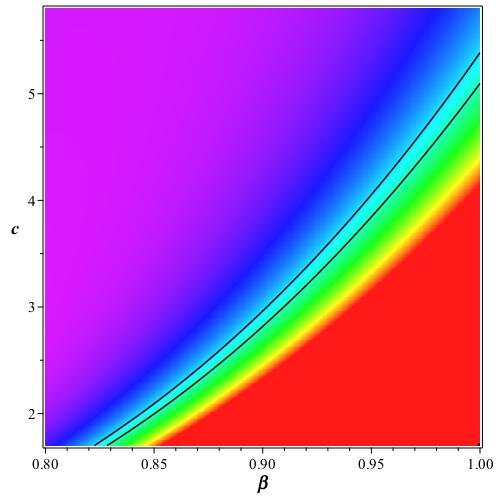
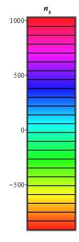
Figure 1: The prediction of the intermediate anisotropic tachyon inflation for the scalar spectral index and tensor-to-scalar ratio in some domains of the model’s parameters space. In the left panel, the region between two solid lines leads to the observationally viable values of $n_{s}$, obtained from Planck2018 TT, TE, EE +lowE+lensing+BK14 +BAO data. In the right panel, the region above the solid line leads to the observationally viable values of $r$ obtained from Planck2018 TT, TE, EE +lowE+lensing+BK14 +BAO data. Also, the region above the dashed line leads to the observationally viable values of $r$ obtained from Planck2018 TT, TE, EE +lowE+lensing+BK18+BAO data.

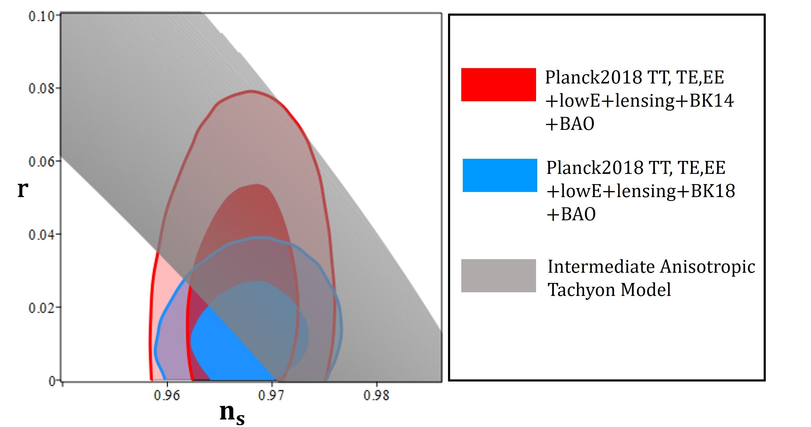
Figure 2: Tensor-to-scalar ratio versus the scalar spectral index for the intermediate anisotropic tachyon inflation, in the background of Planck2018 TT, TE, EE +lowE+lensing+BK14 +BAO and Planck2018 TT, TE, EE +lowE+lensing+BK18 +BAO data.

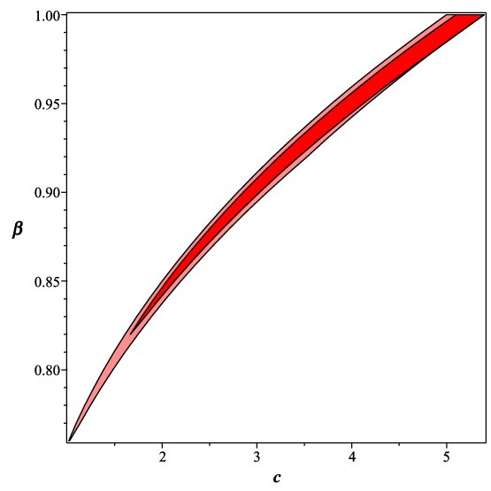
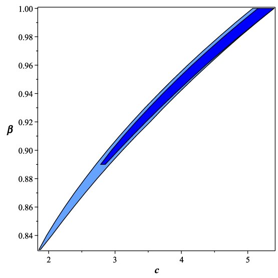
Figure 3: Left panel: the parameters space of $c$ and $\beta$ for the intermediate anisotropic tachyon inflation, leading to observationally viable values of $r-n_{s}$, in confrontation with Planck2018 TT, TE, and EE+lowE+lensing+BAO+BK14 data at $68\%$ CL (dark red) and $95\%$ CL (light red). Right panel: the parameters space of $c$ and $\beta$ for the intermediate anisotropic tachyon inflation, leading to observationally viable values of $r-n_{s}$, in confrontation with Planck2018 TT, TE, and EE+lowE+lensing+BAO+BK18 data at $68\%$ CL (dark blue) and $95\%$ CL (light blue).

Planck collaboration has also released some constraints on the amplitude of the non-gausianity. The constraint on the equilateral amplitude of the non-gaussianity, obtained from Planck2018 TTT, EEE, TTE, and EET data, is $f_{NL}^{equil}=-26\pm 47$ [62]. Now, we consider the following relation between the sound speed and the equilateral amplitude of the non-gaussianity

$$f_{NL}^{equil}=\frac{85}{324}\Bigg{(}1-\frac{1}{c_{s}^{2}}\Bigg{)}\,.$$ (23)

From equations (2) and (23), and by using the observational constraint on the $f_{NL}^{equil}$, we have found that for all values of $0<\beta<1$ and $c>0$ the amplitude of the non-gaussianity in the intermediate anisotropic tachyon inflation is consistent with Planck2018 TTT, EEE, TTE, and EET data. However, we are interested in those values of $c$ and $\beta$ that give observationally viable values of all $n_{s}$, $r$, and $f_{NL}^{equil}$. In this regard, we consider the observationally viable ranges of $c$ and $\beta$, which have been obtained from the viable ranges of $r-n_{s}$ in confrontation with Planck2018 TT, TE, and EE+lowE+lensing+BAO+BK14(18) data. By using these constraints, we have plotted the parameter space $c_{s}-c$ in figure 4. We have also obtained some constraints on the sound speed, for some sample values of $\beta$, that have been summarized in table 2. These constraints on $c$ and $c_{s}$, give us some information about the amplitude of the non-gaussianity. In figure 5 we have plotted the parameter space $f_{NL}^{equil}-c$. This figure shows that for those domains of beta, that lead to the observationally viable values of $r-n_{s}$, the amplitude of the non-gaussianity is ${\cal{O}}(10^{-2}-10^{-1})$. We have also summarized some constraints on the equilateral amplitude of the non-gaussianity in table 2.

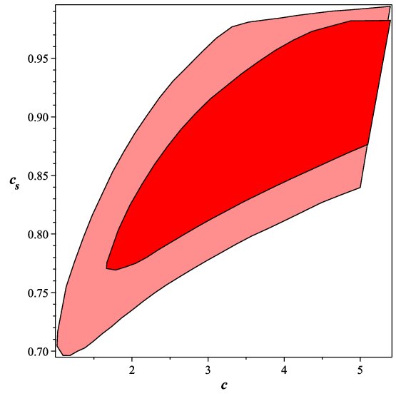
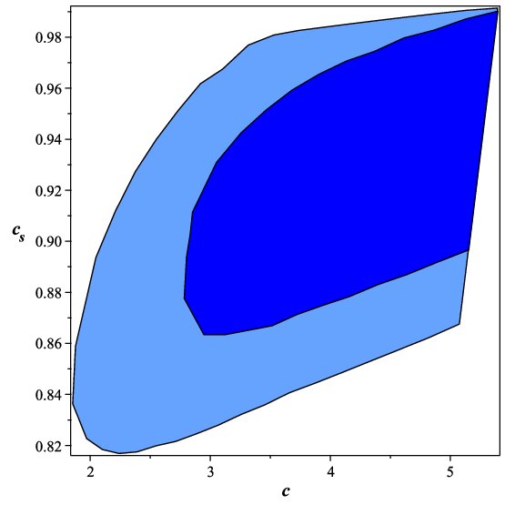
Figure 4: Left panel: the parameter space of $c_{s}$ and $c$ for the intermediate anisotropic tachyon inflation, corresponding to observationally viable values of $r-n_{s}$, obtained from Planck2018 TT, TE, and EE+lowE+lensing+BAO+BK14 data at $68\%$ CL (dark red) and $95\%$ CL (light red). Right panel: the parameter space of $c_{s}$ and $c$ for the intermediate anisotropic tachyon inflation, corresponding to observationally viable values of $r-n_{s}$, obtained from Planck2018 TT, TE, and EE+lowE+lensing+BAO+BK18 data at $68\%$ CL (dark blue) and $95\%$ CL (light blue).

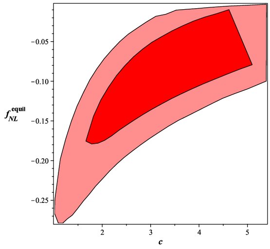
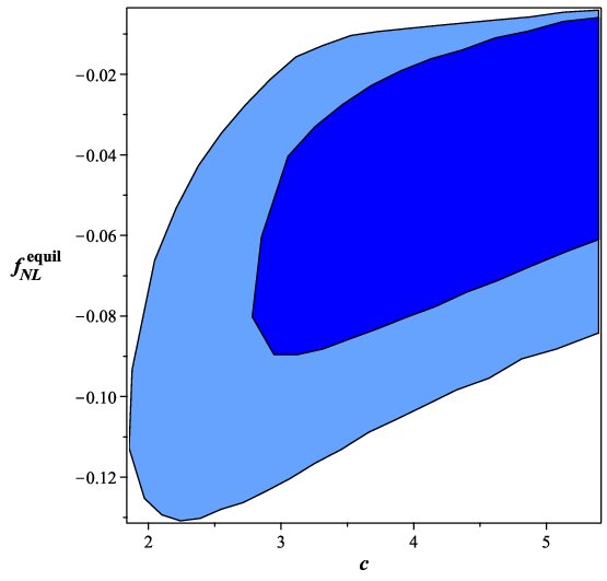
Figure 5: Left panel: the parameter space of $f_{NL}^{equil}$ and $c$ for the intermediate anisotropic tachyon inflation, corresponding to observationally viable values of $c_{s}$, obtained from Planck2018 TT, TE, and EE+lowE+lensing+BAO+BK14 data at $68\%$ CL (dark red) and $95\%$ CL (light red). Right panel: the parameter space of $f_{NL}^{equil}$ and $c$ for the intermediate anisotropic tachyon inflation, corresponding to observationally viable values of $c_{s}$, obtained from Planck2018 TT, TE, and EE+lowE+lensing+BAO+BK18 data at $68\%$ CL (dark blue) and $95\%$ CL (light blue).

Table 1: Ranges of the parameter $c$, for some sample values of $\beta$, in which the tensor-to-scalar ratio and scalar spectral index of the intermediate anisotropic tachyon model are consistent with different data sets.

	Planck2018 TT,TE,EE+lowE	Planck2018 TT,TE,EE+lowE	Planck2018 TT,TE,EE+lowE	Planck2018 TT,TE,EE+lowE
	+lensing+BK14+BAO	+lensing+BK14+BAO	lensing+BK18+BAO	lensing+BK18+BAO
$\beta$	$68\%$ CL	$95\%$ CL	$68\%$ CL	$95\%$ CL
$0.80$	Not consistent	$1.382<c<1.480$	Not consistent	Not consistent
$0.85$	$2.049<c<2.129$	$2.00<c<2.197$	Not consistent	$2.101<c<2.209$
$0.90$	$2.855<c<3.028$	$2.796<c<3.107$	$2.947<c<3.052$	$2.885<c<3.113$
$0.95$	$3.864<c<4.122$	$3.788<c<4.169$	$3.937<c<4.132$	$3.873<c<4.169$

Table 2: Ranges of the observationally viable values of the sound speed and corresponding equilateral amplitude of the non-gaussianity, in the intermediate anisotropic tachyon model and in confrontation with different data sets.

	Planck2018 TT,TE,EE+lowE		Planck2018 TT,TE,EE+lowE		Planck2018 TT,TE,EE+lowE		Planck2018 TT,TE,EE+lowE
	+lensing+BK14+BAO		+lensing+BK14+BAO		lensing+BK18+BAO		lensing+BK18+BAO
$\beta$	$68\%$ CL		$95\%$ CL		$68\%$ CL		$95\%$ CL
$0.80$	Not consistent		$0.159<c_{s}<0.185$		Not consistent		Not consistent
	Not consistent		$-0.268<f_{NL}<-0.131$		Not consistent		Not consistent
$0.85$	$0.176<c_{s}<0.191$		$0.167<c_{s}<0.204$		Not consistent		$0.185<c_{s}<0.207$
	$-0.174<f_{NL}^{equil}<-0.107$		$-0.223<f_{NL}^{equil}<-0.060$		Not consistent		$-0.129<f_{NL}^{equil}<-0.053$
$0.90$	$0.183<c_{s}<0.208$		$0.175<c_{s}<0.219$		$0.196<c_{s}<0.211$		$0.187<c_{s}<0.223$
	$-0.141<f_{NL}^{equil}<-0.050$		$-0.179<f_{NL}^{equil}<-0.018$		$-0.089<f_{NL}^{equil}<-0.040$		$-0.123<f_{NL}^{equil}<-0.008$
$0.95$	$0.190<c_{s}<0.219$		$0.176<c_{s}<0.222$		$0.198<c_{s}<0.220$		$0.188<c_{s}<0.220$
	$-0.109<f_{NL}^{equil}<-0.019$		$-0.142<f_{NL}^{equil}<-0.007$		$-0.080<f_{NL}^{equil}<-0.016$		$-0.105<f_{NL}^{equil}<-0.007$

4 Reheating

When the initial inflation expansion of the universe ends, there should be a phase that by reheating the universe makes it ready for the subsequent evolution. This reheating phase is one important process in the history of the universe and studying its cosmology gives us some interesting information. It is believed that when inflation terminates, the inflaton rolls down to the minimum of its potential and starts oscillating there. The oscillation causes the field to lose its energy and decay to relativistic particles [63, 64]. Considering the fact that at the beginning of inflation, the effective equation of state parameter is equal to -1 and at the end of this era it reaches $-\frac{1}{3}$, it is important to know how the universe should be prepared for the subsequent eras. This would be more important when we consider that the value of the equation of state at the beginning of the radiation dominated phase is $\frac{1}{3}$. It has been shown in Ref. [65] that, in the case of massive inflation, the field initially oscillates at a rate much larger than the expansion rate. This, with a good approximation, leads to a zero effective equation of state at the beginning of the reheating phase. By more oscillating of the field and decaying to other particles, the value of the effective equation of state parameter changes, and at the end of the reheating phase it becomes equal to $\frac{1}{3}$. There are also some other scenarios such as instant reheating [66], tachyon instability [67, 68, 69] and resonance decay [70, 71, 72], where the reheating occurs in a non-perturbative process. To study the reheating phase in the intermediate anisotropic tachyon model, we follow Refs. [73, 74, 75, 76, 77] and find the number of e-folds during the reheating phase ($N_{rh}$) in our model. By starting the definition of the e-folds number as

$$N=\ln\left(\frac{a_{e}}{a_{hc}}\right)\,,$$ (24)

that has been defined between the Hubble crossing ($hc$) of the physical scales and the end ($e$) of inflation, we try to find some expression for $N_{rh}$ in terms of the model’s parameters. Since the scale factor is related to the energy density as $\rho\sim a^{-3(1+\omega_{eff})}$, where $\omega_{eff}$ is the effective equation of state during the reheating, we have

$$N_{rh}=\ln\left(\frac{a_{rh}}{a_{e}}\right)=-\frac{1}{3(1+\omega_{eff})}\ln\left(\frac{\rho_{rh}}{\rho_{e}}\right)\,.$$ (25)

Now, we use the relation between the wave number and the scale factor at the horizon crossing as

$$0=\ln\left(\frac{k_{hc}}{a_{hc}H_{hc}}\right)=\ln\left(\frac{a_{e}}{a_{hc}}\frac{a_{rh}}{a_{e}}\frac{a_{0}}{a_{rh}}\frac{k_{hc}}{a_{0}H_{hc}}\right)\,,$$ (26)

where the subscript “$0$” stands for the current value of the corresponding parameter, we get

$$N+N_{rh}+\ln\left(\frac{k_{hc}}{a_{0}H_{hc}}\right)+\ln\left(\frac{a_{0}}{a_{rh}}\right)=0\,.$$ (27)

If we consider the following relation between the energy density and temperature [75, 77]

$$\rho_{rh}=\frac{\pi^{2}g_{rh}}{30}T_{rh}^{4}\,,$$ (28)

with $g_{rh}$ being the effective number of the relativistic species at the reheating phase, and also [75, 77]

$$\frac{a_{0}}{a_{rh}}=\left(\frac{43}{11g_{rh}}\right)^{-\frac{1}{3}}\frac{T_{rh}}{T_{0}}\,,$$ (29)

we obtain

$$\frac{a_{0}}{a_{rh}}=\left(\frac{43}{11g_{rh}}\right)^{-\frac{1}{3}}T_{0}^{-1}\left(\frac{\pi^{2}g_{rh}}{30\rho_{rh}}\right)^{-\frac{1}{4}}\,.$$ (30)

In our intermediate anisotropic tachyon model, we can write the energy density as

$$\rho=\frac{V\sqrt{18\kappa^{2}\,V+\sum_{i=1}^{3}(\dot{\alpha}^{i})^{2}}}{\sqrt{(18-12\epsilon)\kappa^{2}\,V-\sum_{i=1}^{3}(\dot{\alpha}^{i})^{2}}}\,.$$ (31)

Therefore, at the end of inflation, we have

$$\rho_{e}=\frac{V_{e}\sqrt{18\kappa^{2}\,V_{e}+\sum_{i=1}^{3}(\dot{\alpha}^{i})^{2}}}{\sqrt{6\kappa^{2}\,V_{e}-\sum_{i=1}^{3}(\dot{\alpha}^{i})^{2}}}\,,$$ (32)

which by using equation (25) leads to

$$\rho_{rh}=\Bigg{[}\frac{V_{e}\sqrt{18\kappa^{2}\,V_{e}+\sum_{i=1}^{3}(\dot{\alpha}^{i})^{2}}}{\sqrt{6\kappa^{2}\,V_{e}-\sum_{i=1}^{3}(\dot{\alpha}^{i})^{2}}}\,\Bigg{]}\,\exp\Big{[}-3N_{rh}(1+\omega_{eff})\Big{]}.$$ (33)

From the above equation and also equation (30) we find

$$\ln\left(\frac{a_{0}}{a_{rh}}\right)=-\frac{1}{3}\ln\left(\frac{43}{11g_{rh}}\right)-\frac{1}{4}\ln\left(\frac{\pi^{2}g_{rh}}{30\rho_{rh}}\right)-\ln T_{0}+\frac{1}{4}\ln\Bigg{(}\frac{V_{e}\sqrt{18\kappa^{2}\,V_{e}+\sum_{i=1}^{3}(\dot{\alpha}^{i})^{2}}}{\sqrt{6\kappa^{2}\,V_{e}-\sum_{i=1}^{3}(\dot{\alpha}^{i})^{2}}}\Bigg{)}$$

$$-\frac{3}{4}N_{rh}(1+\omega_{eff})\,.$$ (34)

Now, we find the number of e-folds during the reheating from equations (27) and (4) as

$$N_{rh}=\frac{4}{1-3\omega_{eff}}\Bigg{[}-N-\ln\Big{(}\frac{k_{hc}}{a_{0}T_{0}}\Big{)}-\frac{1}{4}\ln\Big{(}\frac{40}{\pi^{2}g_{rh}}\Big{)}-\frac{1}{3}\ln\Big{(}\frac{11g_{rh}}{43}\Big{)}$$

$$+\frac{1}{2}\ln\Big{(}H^{2}\Big{)}-\frac{1}{4}\ln\Bigg{(}\frac{V_{e}\sqrt{18\kappa^{2}\,V_{e}+\sum_{i=1}^{3}(\dot{\alpha}^{i})^{2}}}{\sqrt{6\kappa^{2}\,V_{e}-\sum_{i=1}^{3}(\dot{\alpha}^{i})^{2}}}\Bigg{)}\Bigg{]}.$$ (35)

Also, from equations (25), (29), and (32) we find the temperature during the reheating phase as

$$T_{rh}=\bigg{(}\frac{30}{\pi^{2}g_{rh}}\bigg{)}^{\frac{1}{4}}\,\Bigg{[}\frac{V_{e}\sqrt{18\kappa^{2}\,V_{e}+\sum_{i=1}^{3}(\dot{\alpha}^{i})^{2}}}{\sqrt{6\kappa^{2}\,V_{e}-\sum_{i=1}^{3}(\dot{\alpha}^{i})^{2}}}\,\Bigg{]}^{\frac{1}{4}}\,\exp\bigg{[}-\frac{3}{4}N_{rh}(1+\omega_{eff})\bigg{]}\,.$$ (36)

To perform a numerical analysis on the reheating parameters, we use the equation (10) and also the general definition of the slow-roll parameter as $\epsilon=-\frac{\dot{H}}{H^{2}}$ to find equation (31) in terms of $\epsilon$. Then, we consider $\epsilon=1$ (corresponding to the end of the inflation) and find equation (32) in terms of the model’s parameters. Also, from equation (18), we can obtain $\epsilon$ and therefore $H^{2}$ in terms of the tensor-to-scalar ratio and substitute it in equation (4). In this way, we can perform some numerical analysis in our model to study the reheating process. The observational constraints on $r$ lead to some constraints on the reheating parameters. We use both Planck2018 TT, TE, and EE+lowE+lensing+BAO+BK14 and Planck2018 TT, TE, and EE+lowE+lensing+BAO+BK18 constraints on the tensor-to-scalar ratio as $r<0.072$ and $r<0.036$, respectively. Figure 6 shows the parameter space of $N_{rh}$ and $\omega_{eff}$ leading to the observationally viable values of the tensor-to-scalar ratio. In this figure, we have adopted two sample values of $c$. As the figure shows, in this model it is possible to have instantaneous reheating where $N_{rh}\rightarrow 0$. We have obtained some constraints on $N_{rh}$, for some sample values of $c$ and $\beta$ that have been summarized in table 3. Also, for consistency with Big-Bang nucleosynthesis, the temperature during the reheating phase should be larger or of the order of $10MeV$. To check this consistency in our model, we have performed some numerical analysis on $T_{rh}$. The result is shown in figure 7, for two sample values of $c$. It seems that this consistency is satisfied in the intermediate anisotropic tachyon inflation. We have also obtained some constraints on the reheating temperature that have been presented in table 4. To show the results of this section more clearly, we have plotted $N_{rh}-r$ and $\log_{10}\Big{(}\frac{T_{rh}}{GeV}\Big{)}-r$ for some adopted values of the equation of state parameter as $\omega_{eff}=-1,-\frac{1}{3},0,1$. The results have been shown in figure 8. This figure shows that all plotted curves meet at one point where $\omega=\frac{1}{3}$ would pass vertically and also it is observationally viable. In fact, this figure shows that instantaneous reheating is possible, at least in some domains of the parameter space. In Ref [78] also, the possibility of having instantaneous reheating in the tachyon model has been shown. According to our study, the intermediate anisotropic inflation gives the viable reheating process after inflation.

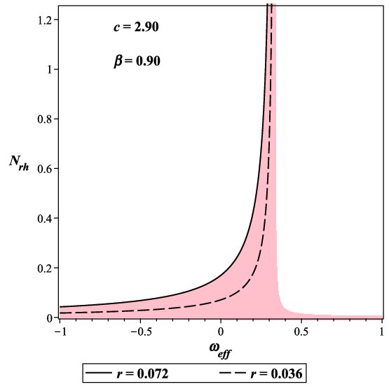
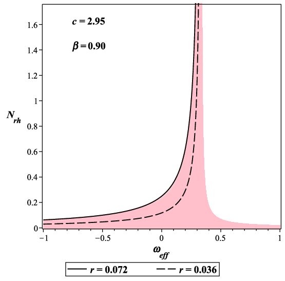
Figure 6: Ranges of the e-folds number and the effective equation of state parameter during the reheating phase for the intermediate anisotropic tachyon inflation, leading to the observationally viable values of the tensor-to-scalar ratio.

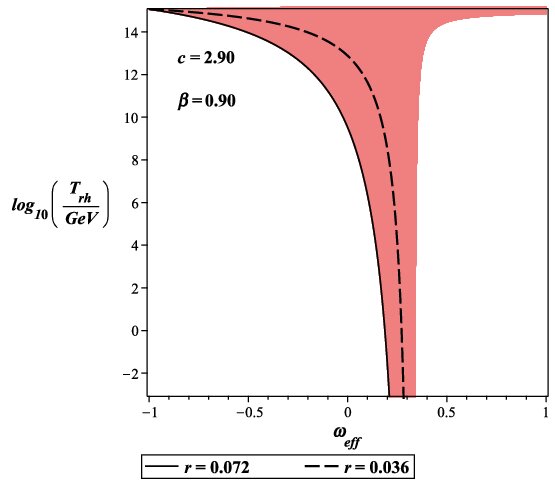
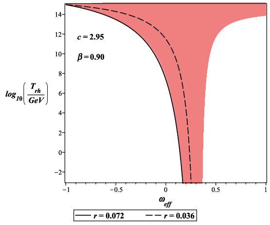
Figure 7: Ranges of the temperature and the effective equation of state parameter during the reheating phase for the intermediate anisotropic tachyon inflation, leading to the observationally viable values of the tensor-to-scalar ratio.

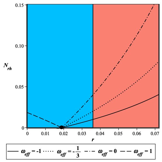
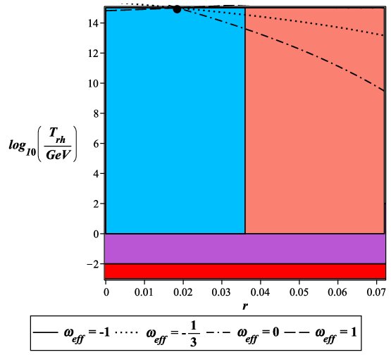
Figure 8: Behavior of the e-folds number and temperature during the reheating phase versus the tensor-to-scalar ratio. The salmon and deep sky blue colors show the ranges of the observationally viable values of the tensor-to-scalar ratio, obtained from Planck2018 TT, TE, and EE+lowE+lensing+BAO+BK14 and Planck2018 TT, TE, and EE+lowE+lensing+BAO+BK18 data, respectively. Note that the salmon region overlaps with some domain of deep sky blue region. In the right panel, the purple region corresponds to the temperatures below the electroweak scale, $T<100$ GeV, and the red region corresponds to the temperatures below the big bang nucleosynthesis scale, $T<10$ MeV.

Table 3: Constraints on the e-folds number during reheating in the intermediate anisotropic tachyon model, obtained from Planck2018 TT, TE, EE+lowE+lensing+BK14 (18)+BAO joint data at $95\%$ CL.

	$\beta$	$c$	$\omega=-1$	$\omega=-\frac{1}{3}$	$\omega=0$
Planck2018 TT, TE, EE+	$0.90$	2.90	$0\leq N_{rh}\leq 0.040$	$0\leq N_{rh}\leq 0.081$	$0\leq N_{rh}\leq 0.171$
lowE+lensing+BK14	$0.90$	2.95	$0\leq N_{rh}\leq 0.058$	$0\leq N_{rh}\leq 0.124$	$0\leq N_{rh}\leq 0.250$
+BAO	$0.90$	3.00	$0\leq N_{rh}\leq 0.075$	$0\leq N_{rh}\leq 0.145$	$0\leq N_{rh}\leq 0.295$
	$0.95$	3.90	$0\leq N_{rh}\leq 0.079$	$0\leq N_{rh}\leq 0.151$	$0\leq N_{rh}\leq 0.301$
	$0.95$	3.95	$0\leq N_{rh}\leq 0.085$	$0\leq N_{rh}\leq 0.157$	$0\leq N_{rh}\leq 0.307$
	$0.95$	4.00	$0\leq N_{rh}\leq 0.091$	$0\leq N_{rh}\leq 0.161$	$0\leq N_{rh}\leq 0.312$
Planck2018 TT, TE, EE+	$0.90$	2.95	$0\leq N_{rh}\leq 0.010$	$0\leq N_{rh}\leq 0.035$	$0\leq N_{rh}\leq 0.039$
lowE+lensing+BK18	$0.90$	3.00	$0\leq N_{rh}\leq 0.026$	$0\leq N_{rh}\leq 0.058$	$0\leq N_{rh}\leq 0.113$
+BAO	$0.90$	3.05	$0\leq N_{rh}\leq 0.064$	$0\leq N_{rh}\leq 0.115$	$0\leq N_{rh}\leq 0.216$
	$0.95$	3.90	$0\leq N_{rh}\leq 0.073$	$0\leq N_{rh}\leq 0.126$	$0\leq N_{rh}\leq 0.230$
	$0.95$	3.95	$0\leq N_{rh}\leq 0.077$	$0\leq N_{rh}\leq 0.131$	$0\leq N_{rh}\leq 0.235$
	$0.95$	4.00	$0\leq N_{rh}\leq 0.083$	$0\leq N_{rh}\leq 0.137$	$0\leq N_{rh}\leq 0.242$

Table 4: Constraints on the temperature during reheating in the intermediate anisotropic tachyon model, obtained from Planck2018 TT, TE, EE+lowE+lensing+BK14 (18)+BAO joint data at $95\%$ CL.

	$\beta$	$c$	$\omega=-1$	$\omega=-\frac{1}{3}$	$\omega=0$
Planck2018 TT, TE, EE+	$0.90$	2.90	$14.99\leq\log_{10}\left(\frac{T_{rh}}{GeV}\right)\leq 15.00$	$13.17\leq\log_{10}\left(\frac{T_{rh}}{GeV}\right)\leq 15.00$	$9.46\leq\log_{10}\left(\frac{T_{rh}}{GeV}\right)\leq 15.00$
lowE+lensing+BK14	$0.90$	2.95	$14.98\leq\log_{10}\left(\frac{T_{rh}}{GeV}\right)\leq 15.00$	$12.43\leq\log_{10}\left(\frac{T_{rh}}{GeV}\right)\leq 15.00$	$7.28\leq\log_{10}\left(\frac{T_{rh}}{GeV}\right)\leq 15.00$
+BAO	$0.90$	3.00	$14.98\leq\log_{10}\left(\frac{T_{rh}}{GeV}\right)\leq 15.00$	$11.65\leq\log_{10}\left(\frac{T_{rh}}{GeV}\right)\leq 15.00$	$6.03\leq\log_{10}\left(\frac{T_{rh}}{GeV}\right)\leq 15.00$
	$0.95$	3.90	$14.97\leq\log_{10}\left(\frac{T_{rh}}{GeV}\right)\leq 15.00$	$10.93\leq\log_{10}\left(\frac{T_{rh}}{GeV}\right)\leq 15.00$	$5.12\leq\log_{10}\left(\frac{T_{rh}}{GeV}\right)\leq 15.00$
	$0.95$	3.95	$14.96\leq\log_{10}\left(\frac{T_{rh}}{GeV}\right)\leq 15.00$	$10.47\leq\log_{10}\left(\frac{T_{rh}}{GeV}\right)\leq 15.00$	$4.05\leq\log_{10}\left(\frac{T_{rh}}{GeV}\right)\leq 15.00$
	$0.95$	4.00	$14.95\leq\log_{10}\left(\frac{T_{rh}}{GeV}\right)\leq 15.00$	$10.00\leq\log_{10}\left(\frac{T_{rh}}{GeV}\right)\leq 15.00$	$2.14\leq\log_{10}\left(\frac{T_{rh}}{GeV}\right)\leq 15.00$
Planck2018 TT, TE, EE+	$0.90$	2.90	$14.99\leq\log_{10}\left(\frac{T_{rh}}{GeV}\right)\leq 15.00$	$14.28\leq\log_{10}\left(\frac{T_{rh}}{GeV}\right)\leq 15.00$	$13.56\leq\log_{10}\left(\frac{T_{rh}}{GeV}\right)\leq 15.00$
lowE+lensing+BK18	$0.90$	2.95	$14.99\leq\log_{10}\left(\frac{T_{rh}}{GeV}\right)\leq 15.00$	$13.77\leq\log_{10}\left(\frac{T_{rh}}{GeV}\right)\leq 15.00$	$11.50\leq\log_{10}\left(\frac{T_{rh}}{GeV}\right)\leq 15.00$
+BAO	$0.90$	3.00	$14.91\leq\log_{10}\left(\frac{T_{rh}}{GeV}\right)\leq 15.00$	$13.15\leq\log_{10}\left(\frac{T_{rh}}{GeV}\right)\leq 15.00$	$10.68\leq\log_{10}\left(\frac{T_{rh}}{GeV}\right)\leq 15.00$
	$0.95$	3.90	$14.95\leq\log_{10}\left(\frac{T_{rh}}{GeV}\right)\leq 15.00$	$12.78\leq\log_{10}\left(\frac{T_{rh}}{GeV}\right)\leq 15.00$	$9.74\leq\log_{10}\left(\frac{T_{rh}}{GeV}\right)\leq 15.00$
	$0.95$	3.95	$14.85\leq\log_{10}\left(\frac{T_{rh}}{GeV}\right)\leq 14.93$	$12.33\leq\log_{10}\left(\frac{T_{rh}}{GeV}\right)\leq 15.00$	$9.01\leq\log_{10}\left(\frac{T_{rh}}{GeV}\right)\leq 15.00$
	$0.95$	4.00	$14.9\leq\log_{10}\left(\frac{T_{rh}}{GeV}\right)\leq 15.00$	$11.73\leq\log_{10}\left(\frac{T_{rh}}{GeV}\right)\leq 15.00$	$8.24\leq\log_{10}\left(\frac{T_{rh}}{GeV}\right)\leq 15.00$

5 Conclusion

In this paper, we have studied the intermediate tachyon inflation in the anisotropic geometry. We have obtained the Friedmann equations in this anisotropic background. Since the Friedmann equations are modified, the effects of the anisotropy are presented in the potential of the model. In this regard, by using the modified potential, we have obtained the slow-roll parameters in the anisotropic tachyon inflation. It has been shown that the anisotropic background changes the slow-roll parameters in the tachyon model. Therefore, the important perturbation parameters, such as the scalar spectral index and the tensor-to-scalar ratio are changed too. This may change the viability of the model. To seek the observational viability of this model, we have considered the intermediate scale factor and obtained the slow-roll parameters in the intermediate anisotropic tachyon inflation. We have analyzed the model numerically and found the prediction of our model for the scalar spectral index and tensor-to-scalar ratio. We have shown that, in some domains of the model’s parameters, the model is observationally viable. To show the viability of the intermediate anisotropic tachyon inflation more clearly, we have plotted the $r-n_{s}$ behavior in the background of Planck2018 TT, TE, EE+lowE+lensing+BK14(18)+BAO data. We have also obtained some constraints on the parameter $c$ that have been summarized in tables. By using the observational constraints, we have plotted the $c-\beta$ parameters space leading to the observationally viable values of $n_{s}$ and $r$, in confrontation with Planck2018 TT, TE, EE+lowE+lensing+BK14(18)+BAO data at $68\%$ and $98\%$ CL. Given that the tensor-to-scalar ratio and sound speed are related, by using the constraints on $r$, we have found the observationally viable ranges of the sound speed. In this way, we have also obtained some constraints on the amplitude of the non-gaussianity in our model. We have shown that the prediction of our model for the equilateral amplitude of the non-gaussianity is of the order of $10^{-2}-10^{-1}$. Finally, we have studied the reheating process after inflation in our setup. By analyzing the number of e-folds and temperature during the reheating, we have obtained some additional information about the model. We have used the observational constraints on the tensor-to-scalar ratio and obtained the viable domains of $N_{rh}-\omega_{eff}$ and $T_{rh}-\omega_{eff}$ parameters space. We have shown in the intermediate anisotropic tachyon inflation, it is possible to have instantaneous reheating. Also, the temperature during the reheating is consistent with Big-Bang nucleosynthesis.

ACKNOWLEDGMENTS
I thank the referee for the very insightful comments that have improved the quality of the paper considerably.

Appendix A

$$\eta=\Bigg{[}4\Bigg{(}2\left(Y+2\dot{H}\right)\left(-6H^{2}+Y\right)^{2}\left(6H^{2}+4\dot{H}+Y\right)\dddot{H}-8\left(\frac{3}{2}H^{2}+Y+\frac{5}{2}\dot{H}\right)\left(-6H^{2}+Y\right)^{2}\ddot{H}^{2}$$

$$-72\Bigg{(}4H\dot{H}^{3}+\left(4H^{3}+\frac{14}{3}YH-\frac{1}{9}{\frac{\rm d}{{\rm d}t}}Y\right)\dot{H}^{2}+\Bigg{(}\Big{(}\frac{1}{18}Y-H^{2}\Big{)}\dot{Y}+6H^{5}+6YH^{3}+\frac{7}{6}Y^{2}H\Bigg{)}\dot{H}$$

$$+\Big{(}-\frac{1}{2}H^{4}-\frac{1}{3}H^{2}Y+\frac{1}{24}Y^{2}\Big{)}\dot{Y}+YH^{3}\left(6H^{2}+Y\right)\Bigg{)}\left(-6H^{2}+Y\right)\ddot{H}+\left(Y+2\dot{H}\right)^{2}\left(Y-6H^{2}\right)$$

$$\left(6H^{2}+4\dot{H}+Y\right)\ddot{Y}+\left(576H^{2}-192Y\right)\dot{H}^{5}+\Bigg{(}96\dot{Y}H-144\left(12H^{2}+Y\right)\left(-4H^{2}+Y\right)\Bigg{)}\dot{H}^{4}$$

$$+\Bigg{(}5184H^{6}+4320FH^{4}-1152Y^{2}H^{2}-24Y^{3}+144\dot{Y}YH-4\dot{Y}^{2}\Bigg{)}\dot{H}^{3}+\Bigg{(}\left(-12H^{2}-4Y\right)\dot{Y}^{2}$$

$$+\Big{(}576YH^{3}-1728H^{5}+24Y^{2}H\Big{)}\dot{Y}-216YH^{2}\Big{(}-12H^{4}-2H^{2}Y+Y^{2}\Big{)}\Bigg{)}\dot{H}^{2}-6\Bigg{(}\big{(}6H^{4}+\frac{1}{3}Y^{2}\big{)}\dot{Y}$$

$$+H\Bigg{(}216H^{6}+36YH^{4}-30Y^{2}H^{2}+Y^{3}\Bigg{)}\Bigg{)}\dot{Y}\dot{H}-\frac{1}{2}\dot{Y}^{2}Y\left(36H^{4}-6H^{2}Y+Y^{2}\right)\Bigg{)}\Bigg{]}$$

$$\times\Bigg{[}\left(6H^{2}+4\dot{H}+Y\right)^{\frac{5}{2}}\left(-6H^{2}+Y\right)^{\frac{3}{2}}\left(Y+2\dot{H}\right)^{2}\Bigg{]}^{-1}\,,$$

where,

$$Y=\sum_{i=1}^{3}(\dot{\alpha}^{i})^{2}$$

Appendix B

$$\zeta=\Bigg{[}\frac{144}{\kappa^{2}}\bigg{(}(2Y-12H^{2})\ddot{H}-24H\dot{H}^{2}+(2\dot{Y}-72H^{3})\dot{H}+Y\dot{Y}\bigg{)}\bigg{(}-\frac{1}{36}\Big{(}(2\dot{H}+Y)^{2}(-6H^{2}+Y)^{3}$$

$$(6H^{2}+4\dot{H}+Y)^{2}(\ddddot{H})\Big{)}+\Big{(}\frac{1}{2}\big{(}\frac{2H^{2}}{3}+Y+\frac{20\dot{H}}{9}\big{)}\big{(}Y-6H^{2}\big{)}\ddot{H}+\frac{8H\dot{H}^{3}}{3}+\big{(}\frac{14YH}{3}-4H^{3}\big{)}\dot{H}^{2}$$

$$+\big{(}\big{(}\frac{Y}{3}-2H^{2}\big{)}\dot{Y}+12H^{5}+\frac{5HY^{2}}{3}\big{)}\dot{H}+\big{(}\frac{5Y^{2}}{36}-H^{4}-\frac{2H^{2}Y}{3}\big{)}\dot{Y}+H^{3}Y\big{(}6H^{2}+Y\big{)}\Big{)}\big{(}2\dot{H}+Y\big{)}$$

$$\big{(}6H^{2}+4\dot{H}+Y\big{)}\big{(}Y-6H^{2}\big{)}^{2}\dddot{H}-\frac{\big{(}2\dot{H}+Y\big{)}^{3}\big{(}Y-6H^{2}\big{)}^{2}\big{(}6H^{2}+4\dot{H}+Y\big{)}^{2}\dddot{Y}}{72}-\frac{65}{36}\Big{(}\frac{328\dot{H}^{2}}{65}$$

$$+\big{(}\frac{216H^{2}}{65}+\frac{292Y}{65}\big{)}\dot{H}+\frac{36H^{4}}{65}+\frac{96H^{2}Y}{65}+Y^{2}\Big{)}\Big{(}Y-6H^{2}\Big{)}^{3}\ddot{H}^{3}+\Big{(}Y-6H^{2}\Big{)}^{2}\Big{(}-24H\dot{H}^{4}$$

$$+\big{(}176H^{3}-\frac{260YH}{3}-\frac{14\dot{Y}}{9}\big{)}\dot{H}^{3}+\big{(}\big{(}\frac{122H^{2}}{3}-\frac{82Y}{9}\big{)}\dot{Y}-204H^{5}+84H^{3}Y-\frac{175HY^{2}}{3}\Big{)}\dot{H}^{2}$$

$$+\Big{(}\big{(}31H^{4}+\frac{91H^{2}Y}{3}-\frac{85Y^{2}}{12}\big{)}\dot{Y}-108H^{7}-288YH^{5}-11H^{3}Y^{2}-\frac{26HY^{3}}{3}\Big{)}\dot{H}+\Big{(}6H^{6}+\frac{25YH^{4}}{2}$$

$$+\frac{11H^{2}Y^{2}}{2}-\frac{107Y^{3}}{72}\Big{)}\dot{Y}-72YH^{7}-84Y^{2}H^{5}-6Y^{3}H^{3}+HY^{4}\Big{)}\ddot{H}^{2}+9\Big{(}\frac{1}{54}\big{(}6H^{2}+4\dot{H}+Y\big{)}$$

$$\big{(}2\dot{H}+Y\big{)}^{2}\Big{(}-6H^{2}+Y\Big{)}\Big{(}-2H^{2}+Y+\frac{4\dot{H}}{3}\Big{)}\ddot{Y}+\Big{(}32H^{2}+\frac{64Y}{27}\Big{)}\dot{H}^{6}+\Big{(}\frac{608H^{4}}{3}+\frac{64Y^{2}}{9}+$$

$$\frac{176H^{2}Y}{3}-\frac{16H\dot{Y}}{27}\Big{)}\dot{H}^{5}+\Big{(}\frac{164Y^{3}}{27}-\frac{22\dot{Y}^{2}}{81}-\frac{112(\frac{6H^{2}}{7}+Y)H\dot{Y}}{27}-240H^{6}+496YH^{4}+\frac{380H^{2}Y^{2}}{9}\Big{)}\dot{H}^{4}$$

$$+\Big{(}\big{(}-\frac{2H^{2}}{9}-\frac{41Y}{81}\big{)}\dot{Y}^{2}+\big{(}\frac{248H^{3}Y}{9}-\frac{242HY^{2}}{27}-\frac{392H^{5}}{3}\big{)}\dot{Y}+192H^{8}+2Y^{4}-64YH^{6}$$

$$+\frac{1040H^{4}Y^{2}}{3}+\frac{164H^{2}Y^{3}}{9}\Big{)}\dot{H}^{3}+\Big{(}\Big{(}2H^{2}Y-7H^{4}-\frac{59Y^{2}}{108}\Big{)}\dot{Y}^{2}+\Big{(}\frac{166H^{3}Y^{2}}{9}-\frac{316YH^{5}}{3}-\frac{17HY^{3}}{3}$$

$$-24H^{7}\Big{)}\dot{Y}+\frac{2Y^{5}}{9}+336YH^{8}+52Y^{2}H^{6}+84Y^{3}H^{4}+\frac{53H^{2}Y^{4}}{9}\Big{)}\dot{H}^{2}+\Big{(}\big{(}\frac{31H^{2}Y^{2}}{18}-\frac{13YH^{4}}{3}-\frac{16H^{6}}{3}$$

$$-\frac{5Y^{3}}{18}\big{)}\dot{Y}^{2}+\Big{(}20YH^{7}-\frac{100Y^{2}H^{5}}{3}+\frac{5Y^{3}H^{3}}{9}-\frac{59HY^{4}}{54}+24H^{9}\Big{)}\dot{Y}+\Big{(}6H^{2}+Y\Big{)}Y^{2}\Big{(}20H^{4}$$

$$-\frac{4H^{2}Y}{3}+Y^{2}\Big{)}H^{2}\Big{)}\dot{H}-\frac{8}{9}\Big{(}\big{(}\frac{9H^{8}}{8}+\frac{9YH^{6}}{4}+\frac{21H^{4}Y^{2}}{32}-\frac{19H^{2}Y^{3}}{48}+\frac{Y^{4}}{18}\big{)}\dot{Y}-27YH^{9}-9Y^{2}H^{7}+\frac{21Y^{3}H^{5}}{4}$$

$$+Y^{4}H^{3}\Big{)}\dot{Y}\Bigg{)}\big{(}-6H^{2}+Y\big{)}\ddot{H}+\frac{1}{6}\bigg{(}\big{(}6H^{2}+4\dot{H}+Y\big{)}\big{(}2\dot{H}+Y\big{)}^{2}\big{(}-6H^{2}+Y\big{)}\Big{(}-24H\dot{H}^{3}+$$

$$\big{(}-84H^{3}-10YH+2\dot{Y}\big{)}\dot{H}^{2}+\big{(}\big{(}3H^{2}+\frac{3Y}{2}\big{)}\dot{Y}+YH\big{(}-42H^{2}+Y\big{)}\big{)}\dot{H}+\frac{5}{12}\dot{Y}\big{(}\frac{72H^{4}}{5}$$

$$-\frac{6H^{2}Y}{5}+Y^{2}\big{)}\Big{)}\ddot{Y}\bigg{)}+\Big{(}384H^{3}+768YH\Big{)}\dot{H}^{8}+\Big{(}4800H^{3}Y-\big{(}864H^{2}+64Y\big{)}\dot{Y}+1280HY^{2}\Big{)}$$

$$\dot{H}^{7}+\Big{(}104H\dot{Y}^{2}-\big{(}3552H^{4}+1760H^{2}Y+128Y^{2}\big{)}\dot{Y}-19008H^{7}+14976YH^{5}+5232H^{3}Y^{2}$$

$$+880HY^{3}\Big{)}\dot{H}^{6}+\Big{(}-\frac{26\dot{Y}^{3}}{9}+\big{(}304H^{3}+\frac{628YH}{3}\big{)}\dot{Y}^{2}-\big{(}\frac{268Y^{3}}{3}+4752H^{6}+1572H^{2}Y^{2}+5280YH^{4}\big{)}\dot{Y}$$

$$+5184H^{9}-24192YH^{7}+19440Y^{2}H^{5}+1680Y^{3}H^{3}+328HY^{4}\Big{)}\dot{H}^{5}+\Big{(}\big{(}-6H^{2}-\frac{56Y}{9}\big{)}\dot{Y}^{3}+\Big{(}36H^{5}$$

$$+\frac{479HY^{2}}{3}+596H^{3}Y\Big{)}\dot{Y}^{2}+\Big{(}11232H^{8}-11880YH^{6}-2088H^{4}Y^{2}-778H^{2}Y^{3}-26Y^{4}\Big{)}\dot{Y}+5184YH^{9}$$

$$-9936Y^{2}H^{7}+8208Y^{3}H^{5}+36Y^{4}H^{3}+68Y^{5}H\Big{)}\dot{H}^{4}+\Big{(}\Big{(}H^{4}-\frac{187Y^{2}}{36}-\frac{37H^{2}Y}{3}\Big{)}\dot{Y}^{3}+\Big{(}756H^{7}-324YH^{5}$$

$$+501H^{3}Y^{2}+52HY^{3}\Big{)}\dot{Y}^{2}+\Big{(}7776H^{10}-\frac{8Y^{5}}{3}-211H^{2}Y^{4}+24Y^{3}H^{4}+6480YH^{8}-7308Y^{2}H^{6}\Big{)}\dot{Y}$$

$$+6HY^{2}\big{(}216H^{8}-216YH^{6}+186H^{4}Y^{2}-6H^{2}Y^{3}+Y^{4}\big{)}\Big{)}\dot{H}^{3}-\frac{1}{2}\Big{(}49\Big{(}\big{(}-\frac{12H^{6}}{7}+\frac{39YH^{4}}{49}+\frac{12H^{2}Y^{2}}{49}$$

$$+\frac{163Y^{3}}{1764}\big{)}\dot{Y}^{2}-\frac{10\Big{(}\frac{756H^{8}}{5}+\frac{252YH^{6}}{5}-45H^{4}Y^{2}+\frac{192H^{2}Y^{3}}{5}+Y^{4}\Big{)}H\dot{Y}}{49}+H^{2}Y\Big{(}-\frac{7776H^{8}}{49}-\frac{864YH^{6}}{49}$$

$$+\frac{2556H^{4}Y^{2}}{49}-\frac{192H^{2}Y^{3}}{49}+Y^{4}\Big{)}\Big{)}\dot{Y}\dot{H}^{2}\Big{)}-\frac{1}{12}\Big{(}5\big{(}\big{(}\frac{4Y^{4}}{3}-\frac{324H^{8}}{5}-\frac{288YH^{6}}{5}+\frac{189H^{4}Y^{2}}{5}$$

$$+\frac{3H^{2}Y^{3}}{5}\big{)}\dot{Y}+H\Big{(}-\frac{3888H^{10}}{5}-\frac{1296YH^{8}}{5}-\frac{324Y^{2}H^{6}}{5}+\frac{504Y^{3}H^{4}}{5}-66H^{2}Y^{4}+Y^{5}\Big{)}\big{)}\dot{Y}^{2}\dot{H}\Big{)}\bigg{)}$$

$$-\frac{Y\Big{(}-216H^{8}-24YH^{6}+46H^{4}Y^{2}-\frac{10H^{2}Y^{3}}{3}+Y^{4}\Big{)}\dot{Y}^{3}}{16}\Big{]}\Big{[}\Big{(}2\dot{H}+Y\Big{)}^{4}\Big{(}6H^{2}+4\dot{H}+Y\Big{)}^{5}$$

$$\Big{(}-6H^{2}+Y\Big{)}^{3}\Big{]}^{-1}$$

where,

$$Y=\sum_{i=1}^{3}(\dot{\alpha}^{i})^{2}.$$

Appendix C

$$\eta=-\Bigg{[}5184\Bigg{(}\frac{b^{\frac{10}{\beta}}\beta^{4}\Big{(}\beta-1\Big{)}^{3}c^{2}\Big{(}\beta^{2}-2\beta+\frac{4}{3}\Big{)}{\mathrm{e}}^{24N}N^{\frac{2+5\beta}{\beta}}}{18}+\frac{\Big{(}\beta-\frac{2}{3}\Big{)}\beta^{2}\Big{(}\beta-1\Big{)}^{3}c^{4}{\mathrm{e}}^{18N}\Big{(}\beta-2\Big{)}b^{\frac{8}{\beta}}N^{\frac{4+3\beta}{\beta}}}{216}$$

$$+\frac{35\beta^{3}\Big{(}\beta-1\Big{)}^{2}c^{4}\Big{(}\beta^{2}-\frac{94}{35}\beta+\frac{68}{35}\Big{)}{\mathrm{e}}^{18N}b^{\frac{8}{\beta}}N^{\frac{4+4\beta}{\beta}}}{216}+\frac{11b^{\frac{10}{\beta}}\beta^{5}\Big{(}\beta-1\Big{)}^{3}\Big{(}\beta-\frac{2}{11}\Big{)}c^{2}{\mathrm{e}}^{24N}N^{\frac{2+6\beta}{\beta}}}{18}$$

$$+\frac{2\Big{(}\beta^{2}+\frac{1}{2}\beta-2\Big{)}b^{\frac{10}{\beta}}\beta^{6}\Big{(}\beta-1\Big{)}c^{2}{\mathrm{e}}^{24N}N^{\frac{2+7\beta}{\beta}}}{3}+\frac{23\beta^{4}\Big{(}\beta-1\Big{)}c^{4}\Big{(}\beta^{2}-\frac{53}{23}\beta+\frac{31}{23}\Big{)}{\mathrm{e}}^{18N}b^{\frac{8}{\beta}}N^{\frac{4+5\beta}{\beta}}}{18}$$

$$+\frac{b^{\frac{6}{\beta}}c^{6}\beta\,{\mathrm{e}}^{12N}\Big{(}\beta-2\Big{)}\Big{(}\beta-1\Big{)}^{2}N^{\frac{6+2\beta}{\beta}}}{216}+\frac{5b^{\frac{6}{\beta}}\beta^{2}\Big{(}\beta-1\Big{)}c^{6}{\mathrm{e}}^{12N}\Big{(}\beta^{2}-2\beta+\frac{6}{5}\Big{)}N^{\frac{3\beta+6}{\beta}}}{108}-\frac{5}{2}b^{\frac{10}{\beta}}\beta^{7}\Big{(}\beta-1\Big{)}$$

$$c^{2}\Big{(}\beta-\frac{8}{5}\Big{)}{\mathrm{e}}^{24N}N^{\frac{2+8\beta}{\beta}}+\frac{41\beta^{5}\Big{(}\beta-1\Big{)}\Big{(}\beta-\frac{38}{41}\Big{)}c^{4}{\mathrm{e}}^{18N}b^{\frac{8}{\beta}}N^{\frac{4+6\beta}{\beta}}}{12}+\frac{23b^{\frac{6}{\beta}}\beta^{3}\Big{(}\beta-1\Big{)}c^{6}{\mathrm{e}}^{12N}\Big{(}\beta-\frac{36}{23}\Big{)}N^{\frac{6+4\beta}{\beta}}}{72}$$

$$+\frac{b^{\frac{4}{\beta}}\beta\,c^{8}{\mathrm{e}}^{6N}\Big{(}6+\beta\Big{)}\Big{(}\beta-1\Big{)}N^{\frac{8+2\beta}{\beta}}}{432}-3b^{\frac{10}{\beta}}c^{2}{\mathrm{e}}^{24N}\beta^{8}\Big{(}\beta-1\Big{)}N^{\frac{2+9\beta}{\beta}}+2b^{\frac{8}{\beta}}c^{4}\beta^{6}{\mathrm{e}}^{18N}\Big{(}\beta-1\Big{)}N^{\frac{4+7\beta}{\beta}}$$

$$+b^{\frac{6}{\beta}}c^{6}\beta^{4}{\mathrm{e}}^{12N}\Big{(}\beta-1\Big{)}N^{\frac{6+5\beta}{\beta}}-\frac{b^{\frac{4}{\beta}}\beta^{2}c^{8}{\mathrm{e}}^{6N}\Big{(}\beta-1\Big{)}N^{\frac{8+3\beta}{\beta}}}{72}+\frac{b^{\frac{2}{\beta}}N^{\frac{2\beta+10}{\beta}}\beta\,c^{10}}{144}+\frac{3b^{\frac{6}{\beta}}N^{\frac{6+6\beta}{\beta}}c^{6}\beta^{5}{\mathrm{e}}^{12N}}{4}$$

$$-\frac{b^{\frac{4}{\beta}}N^{\frac{4\beta+8}{\beta}}\beta^{3}c^{8}{\mathrm{e}}^{6N}}{24}+\Big{(}\beta-1\Big{)}\bigg{(}-\frac{b^{\frac{4}{\beta}}c^{8}{\mathrm{e}}^{6N}\Big{(}\beta-2\Big{)}\Big{(}\beta-3\Big{)}N^{\frac{8+\beta}{\beta}}}{1296}+\frac{b^{\frac{2}{\beta}}N^{\frac{10+\beta}{\beta}}c^{10}}{432}+\beta^{7}\Big{(}\beta-1\Big{)}N^{7}{\mathrm{e}}^{30N}b^{\frac{12}{\beta}}$$

$$\Big{(}\frac{2}{9}+\Big{(}N^{2}+\frac{1}{2}N+\frac{1}{6}\Big{)}\beta^{2}+\Big{(}-N-\frac{7}{18}\Big{)}\beta\Big{)}\bigg{)}\Bigg{)}\beta\,{\mathrm{e}}^{6N}\Bigg{]}\Bigg{[}\Big{(}6\beta^{2}N^{2}b^{\frac{2}{\beta}}{\mathrm{e}}^{6N}-c^{2}N^{\frac{2}{\beta}}\Big{)}^{\frac{3}{2}}\Big{(}6\beta N\,{\mathrm{e}}^{6N}\Big{(}(N+\frac{2}{3})\beta-\frac{2}{3}\Big{)}$$

$$b^{\frac{2}{\beta}}+c^{2}N^{\frac{2}{\beta}}\Big{)}^{\frac{5}{2}}\Big{(}2N\beta\,{\mathrm{e}}^{6N}\Big{(}\beta-1\Big{)}b^{\frac{2}{\beta}}+c^{2}N^{\frac{2}{\beta}}\Big{)}^{2}\Bigg{]}^{-1}$$

Appendix D

$$\zeta=\Bigg{[}{\mathrm{e}}^{12N}\Big{(}-10b^{\frac{6}{\beta}}c^{18}{\mathrm{e}}^{6N}\beta(\beta-2)(\beta-3)N^{\frac{18+3\beta}{\beta}}+\frac{b^{\frac{8}{\beta}}c^{16}{\mathrm{e}}^{12N}(\beta-1)(\beta-3)(\beta-4)(\beta-2)^{2}N^{\frac{16+2\beta}{\beta}}}{9}$$

$$+5544c^{16}b^{\frac{8}{\beta}}\Big{(}\beta-\frac{113}{77}\Big{)}{\mathrm{e}}^{12N}\beta^{4}N^{\frac{16+6\beta}{\beta}}-\frac{2b^{\frac{6}{\beta}}c^{18}{\mathrm{e}}^{6N}\Big{(}\beta-2\Big{)}\Big{(}\beta^{2}-5\beta+7\Big{)}N^{\frac{18+2\beta}{\beta}}}{3}+203148c^{12}{\mathrm{e}}^{24N}\Big{(}\beta^{3}$$

$$-\frac{16583}{5643}\beta^{2}+\frac{16540}{5643}\beta-\frac{5576}{5643}\Big{)}b^{\frac{12}{\beta}}\beta^{6}N^{\frac{8\beta+12}{\beta}}-200b^{\frac{16}{\beta}}c^{8}\Big{(}\beta-2\Big{)}\Big{(}\beta^{3}-\frac{14}{5}\beta^{2}+\frac{108}{25}\beta-\frac{56}{15}\Big{)}{\mathrm{e}}^{36N}\beta^{5}\Big{(}\beta-1\Big{)}^{4}$$

$$N^{\frac{8+7\beta}{\beta}}+164304b^{\frac{16}{\beta}}c^{8}{\mathrm{e}}^{36N}\beta^{7}\Big{(}\beta^{4}-\frac{679}{163}\beta^{3}+\frac{7428}{1141}\beta^{2}-\frac{15544}{3423}\beta+\frac{1384}{1141}\Big{)}\Big{(}\beta-1\Big{)}^{2}N^{\frac{8+9\beta}{\beta}}-\frac{1088}{3}b^{\frac{18}{\beta}}c^{6}\Big{(}\beta-2\Big{)}$$

$$\beta^{6}{\mathrm{e}}^{42N}\Big{(}\beta-1\Big{)}^{5}\Big{(}\beta^{3}-\frac{70}{17}\beta^{2}+\frac{108}{17}\beta-\frac{64}{17}\Big{)}N^{\frac{6+8\beta}{\beta}}-5396b^{\frac{16}{\beta}}\Big{(}\beta^{3}-\frac{2922}{1349}\beta^{2}+\frac{388}{1349}\beta+\frac{72}{71}\Big{)}c^{8}\Big{(}\beta-2\Big{)}{\mathrm{e}}^{36N}\beta^{6}$$

$$\Big{(}\beta-1\Big{)}^{3}N^{\frac{8+8\beta}{\beta}}-7264b^{\frac{18}{\beta}}c^{6}\Big{(}\beta^{3}-\frac{722}{227}\beta^{2}+\frac{616}{227}\beta-\frac{64}{227}\Big{)}\Big{(}\beta-2\Big{)}\beta^{7}{\mathrm{e}}^{42N}\Big{(}\beta-1\Big{)}^{4}N^{\frac{6+9\beta}{\beta}}+8b^{\frac{16}{\beta}}c^{8}\Big{(}\beta-2\Big{)}^{2}$$

$$\Big{(}\beta^{2}-\frac{20}{9}\beta+\frac{20}{9}\Big{)}{\mathrm{e}}^{36N}\beta^{4}(\beta-1)^{5}N^{\frac{8+6\beta}{\beta}}+N^{\frac{20+2\beta}{\beta}}c^{20}(\beta-2)b^{\frac{4}{\beta}}-559872\Big{(}\frac{64}{81}+\Big{(}N^{3}+\frac{53}{18}N^{2}+\frac{13}{9}N+\frac{7}{27}\Big{)}\beta^{4}$$

$$+\Big{(}-\frac{8}{3}N^{3}-\frac{22}{3}N^{2}-\frac{55}{9}N-\frac{118}{81}\Big{)}\beta^{3}+\Big{(}\frac{16}{3}N^{2}+\frac{74}{9}N+\frac{79}{27}\Big{)}\beta^{2}+\Big{(}-\frac{32N}{9}-\frac{68}{27}\Big{)}\beta\Big{)}b^{\frac{24}{\beta}}N^{14}\beta^{13}{\mathrm{e}}^{60N}(\beta-1)^{3}$$

$$\Big{(}-\frac{2}{3}+\Big{(}N+\frac{1}{2}\Big{)}\beta\Big{)}\Big{)}\Big{(}\beta-1\Big{)}+960\Big{(}\beta-4\Big{)}c^{4}\Big{(}\beta-2\Big{)}^{2}\Big{(}\beta-\frac{8}{5}\Big{)}\beta^{8}{\mathrm{e}}^{48N}b^{\frac{20}{\beta}}\Big{(}\beta-1\Big{)}^{6}N^{\frac{4+10\beta}{\beta}}-\frac{2}{3}b^{\frac{10}{\beta}}c^{14}{\mathrm{e}}^{18N}\beta$$

$$\Big{(}2+\beta\Big{)}\Big{(}\beta-3\Big{)}\Big{(}\beta-2\Big{)}^{2}\Big{(}\beta-1\Big{)}^{3}N^{\frac{14+3\beta}{\beta}}+7838208b^{\frac{18}{\beta}}c^{6}{\mathrm{e}}^{42N}\beta^{14}\Big{(}\beta-1\Big{)}^{2}N^{\frac{6+16\beta}{\beta}}-1119744b^{\frac{22}{\beta}}c^{2}{\mathrm{e}}^{54N}\beta^{17}$$

$$\Big{(}\beta-1\Big{)}^{3}N^{\frac{2+18\beta}{\beta}}+1679616b^{\frac{20}{\beta}}c^{4}\beta^{16}{\mathrm{e}}^{48N}\Big{(}\beta-1\Big{)}^{2}N^{\frac{4+18\beta}{\beta}}+21928320b^{\frac{18}{\beta}}c^{6}\beta^{12}\Big{(}\beta^{2}-\frac{1502}{705}\beta+\frac{812}{705}\Big{)}{\mathrm{e}}^{42N}$$

$$\Big{(}\beta-1\Big{)}^{2}N^{\frac{6+14\beta}{\beta}}+31850496\Big{(}\beta^{3}-\frac{799}{256}\beta^{2}+\frac{1693}{512}\beta-\frac{153}{128}\Big{)}c^{4}\beta^{13}{\mathrm{e}}^{48N}b^{\frac{20}{\beta}}\Big{(}\beta-1\Big{)}^{2}N^{\frac{4+15\beta}{\beta}}+13115520b^{\frac{18}{\beta}}c^{6}$$

$$\Big{(}\beta^{3}-\frac{3934}{1265}\beta^{2}+\frac{4083}{1265}\beta-\frac{284}{253}\Big{)}\beta^{11}{\mathrm{e}}^{42N}\Big{(}\beta-1\Big{)}^{2}N^{\frac{6+13\beta}{\beta}}+3234816b^{\frac{16}{\beta}}c^{8}{\mathrm{e}}^{36N}\beta^{9}\Big{(}\beta-1\Big{)}^{2}\Big{(}\beta^{3}-\frac{1325}{468}\beta^{2}$$

$$+\frac{4837}{1872}\beta-\frac{173}{234}\Big{)}N^{\frac{8+11\beta}{\beta}}+653472\,{\mathrm{e}}^{30N}b^{\frac{14}{\beta}}c^{10}\Big{(}\beta^{3}-\frac{6812}{2269}\beta^{2}+\frac{6899}{2269}\beta-\frac{2352}{2269}\Big{)}\beta^{7}\Big{(}\beta-1\Big{)}^{2}N^{\frac{10+9\beta}{\beta}}+30000$$

$$c^{12}{\mathrm{e}}^{24N}b^{\frac{12}{\beta}}\Big{(}\beta^{3}-\frac{399}{125}\beta^{2}+\frac{2153}{625}\beta-\frac{162}{125}\Big{)}\beta^{5}\Big{(}\beta-1\Big{)}^{2}N^{\frac{12+7\beta}{\beta}}+17879616c^{4}\Big{(}\beta^{4}-\frac{14470}{3449}\beta^{3}+\frac{22895}{3449}\beta^{2}$$

$$-\frac{16248}{3449}\beta+\frac{4380}{3449}\Big{)}\beta^{12}{\mathrm{e}}^{48N}b^{\frac{20}{\beta}}\Big{(}\beta-1\Big{)}^{2}N^{\frac{4+14\beta}{\beta}}+1229760b^{\frac{16}{\beta}}c^{8}\Big{(}\beta^{4}-\frac{32769}{8540}\beta^{3}+\frac{9259}{1708}\beta^{2}-\frac{7094}{2135}\beta+\frac{1576}{2135}\Big{)}$$

$${\mathrm{e}}^{36N}\beta^{8}\Big{(}\beta-1\Big{)}^{2}N^{\frac{8+10\beta}{\beta}}+1628784c^{4}\beta^{10}{\mathrm{e}}^{48N}b^{\frac{20}{\beta}}\Big{(}\beta^{4}-\frac{48536}{11311}\beta^{3}+\frac{78064}{11311}\beta^{2}-\frac{55120}{11311}\beta+\frac{14144}{11311}\Big{)}\Big{(}\beta-1\Big{)}^{4}$$

$$N^{\frac{4+12\beta}{\beta}}+919296b^{\frac{22}{\beta}}\Big{(}\beta^{4}-\frac{477}{266}\beta^{3}-\frac{103}{133}\beta^{2}+\frac{362}{133}\beta-\frac{8}{7}\Big{)}c^{2}{\mathrm{e}}^{54N}\beta^{12}\Big{(}\beta-1\Big{)}^{4}N^{\frac{2+14\beta}{\beta}}+198528b^{\frac{18}{\beta}}c^{6}\Big{(}\beta^{4}$$

$$-\frac{4115}{1034}\beta^{3}+\frac{2947}{517}\beta^{2}-\frac{1761}{517}\beta+\frac{360}{517}\Big{)}\beta^{8}{\mathrm{e}}^{42N}\Big{(}\beta-1\Big{)}^{4}N^{\frac{6+10\beta}{\beta}}+1752192b^{\frac{22}{\beta}}c^{2}\Big{(}\beta^{4}-\frac{181}{169}\beta^{3}-\frac{426}{169}\beta^{2}+\frac{648}{169}\beta$$

$$-\frac{200}{169}\Big{)}{\mathrm{e}}^{54N}\beta^{13}\Big{(}\beta-1\Big{)}^{3}N^{\frac{2+15\beta}{\beta}}+1664064\,{\mathrm{e}}^{30N}b^{\frac{14}{\beta}}\Big{(}\beta-\frac{105}{107}\Big{)}c^{10}\beta^{10}\Big{(}\beta-1\Big{)}N^{\frac{10+12\beta}{\beta}}+364176c^{12}{\mathrm{e}}^{24N}b^{\frac{12}{\beta}}$$

$$\beta^{8}\Big{(}\beta-\frac{301}{281}\Big{)}(\beta-1)N^{\frac{12+10\beta}{\beta}}+84024c^{14}\Big{(}\beta-\frac{314}{389}\Big{)}{\mathrm{e}}^{18N}\beta^{6}b^{\frac{10}{\beta}}(\beta-1)N^{\frac{14+8\beta}{\beta}}-18b^{\frac{6}{\beta}}c^{18}{\mathrm{e}}^{6N}\beta^{2}(\beta-1)(\beta-8)$$

$$N^{\frac{18+4\beta}{\beta}}+91272\,{\mathrm{e}}^{30N}b^{\frac{14}{\beta}}c^{10}\beta^{6}\Big{(}\beta-1\Big{)}^{2}\Big{(}\beta^{4}-\frac{16639}{3803}\beta^{3}+\frac{27936}{3803}\beta^{2}-\frac{21372}{3803}\beta+\frac{6296}{3803}\Big{)}N^{\frac{10+8\beta}{\beta}}+2083968b^{\frac{22}{\beta}}c^{2}$$

$${\mathrm{e}}^{54N}\beta^{14}\Big{(}\beta^{3}+\frac{16}{67}\beta^{2}-\frac{176}{67}\beta+\frac{64}{67}\Big{)}\Big{(}\beta-1\Big{)}^{3}N^{\frac{2+16\beta}{\beta}}+1615968b^{\frac{18}{\beta}}c^{6}\beta^{9}{\mathrm{e}}^{42N}\Big{(}\beta^{4}-\frac{21671}{5611}\beta^{3}+\frac{30606}{5611}\beta^{2}$$

$$-\frac{18436}{5611}\beta+\frac{3856}{5611}\Big{)}\Big{(}\beta-1\Big{)}^{3}N^{\frac{6+11\beta}{\beta}}+6426432c^{4}\beta^{11}{\mathrm{e}}^{48N}\Big{(}\beta^{4}-\frac{15779}{3719}\beta^{3}+\frac{25320}{3719}\beta^{2}-\frac{18120}{3719}\beta+\frac{4848}{3719}\Big{)}b^{\frac{20}{\beta}}$$

$$(\beta-1)^{3}N^{\frac{4+13\beta}{\beta}}+4898880\Big{(}\beta-\frac{16}{15}\Big{)}b^{\frac{16}{\beta}}c^{8}{\mathrm{e}}^{36N}\beta^{12}(\beta-1)N^{\frac{8+14\beta}{\beta}}+208320c^{4}\beta^{9}{\mathrm{e}}^{48N}b^{\frac{20}{\beta}}(\beta-1)^{5}\Big{(}\beta^{4}-\frac{32}{7}\beta^{3}$$

$$+\frac{8444}{1085}\beta^{2}-\frac{6256}{1085}\beta+\frac{1664}{1085}\Big{)}N^{\frac{4+11\beta}{\beta}}+343872b^{\frac{22}{\beta}}c^{2}\Big{(}\beta^{4}-\frac{1856}{597}\beta^{3}+\frac{1600}{597}\beta^{2}+\frac{32}{199}\beta-\frac{448}{597}\Big{)}{\mathrm{e}}^{54N}\beta^{11}(\beta-1)^{5}$$

$$N^{\frac{2+13\beta}{\beta}}+5403456b^{\frac{18}{\beta}}c^{6}\Big{(}\beta^{4}-\frac{12466}{3127}\beta^{3}+\frac{18567}{3127}\beta^{2}-\frac{12146}{3127}\beta+\frac{2912}{3127}\Big{)}\beta^{10}{\mathrm{e}}^{42N}\Big{(}\beta-1\Big{)}^{2}N^{\frac{6+12\beta}{\beta}}+8040c^{14}$$

$${\mathrm{e}}^{18N}\beta^{4}b^{\frac{10}{\beta}}\Big{(}\beta^{3}-\frac{1106}{335}\beta^{2}+\frac{1199}{335}\beta-\frac{434}{335}\Big{)}\Big{(}\beta-1\Big{)}N^{\frac{14+6\beta}{\beta}}+30839616c^{4}\Big{(}\beta^{2}-\frac{1408}{661}\beta+\frac{768}{661}\Big{)}\beta^{14}{\mathrm{e}}^{48N}b^{\frac{20}{\beta}}$$

$$\Big{(}\beta-1\Big{)}^{2}N^{\frac{4+16\beta}{\beta}}+5444496b^{\frac{16}{\beta}}c^{8}{\mathrm{e}}^{36N}\beta^{10}\Big{(}\beta^{3}-\frac{12141}{4201}\beta^{2}+\frac{11684}{4201}\beta-\frac{3756}{4201}\Big{)}\Big{(}\beta-1\Big{)}N^{\frac{8+12\beta}{\beta}}+1977696\,{\mathrm{e}}^{30N}$$

$$b^{\frac{14}{\beta}}c^{10}\Big{(}\beta^{2}-\frac{1489}{763}\beta+\frac{732}{763}\Big{)}\beta^{9}(\beta-1)N^{\frac{10+11\beta}{\beta}}+13996800c^{4}\beta^{15}{\mathrm{e}}^{48N}b^{\frac{20}{\beta}}\Big{(}\beta-\frac{28}{25}\Big{)}(\beta-1)^{2}N^{\frac{4+17\beta}{\beta}}+6578496$$

$$b^{\frac{16}{\beta}}c^{8}{\mathrm{e}}^{36N}\beta^{11}\Big{(}\beta^{2}-\frac{865}{423}\beta+\frac{446}{423}\Big{)}\Big{(}\beta-1\Big{)}N^{\frac{8+13\beta}{\beta}}+1212c^{16}b^{\frac{8}{\beta}}{\mathrm{e}}^{12N}\beta^{3}\Big{(}\beta^{2}-\frac{261}{101}\beta+\frac{180}{101}\Big{)}\Big{(}\beta-1\Big{)}N^{\frac{16+5\beta}{\beta}}$$

$$+44784c^{14}\Big{(}\beta^{2}-2\beta+\frac{313}{311}\Big{)}{\mathrm{e}}^{18N}\beta^{5}b^{\frac{10}{\beta}}\Big{(}\beta-1\Big{)}N^{\frac{14+7\beta}{\beta}}+20528640\Big{(}\beta-\frac{12}{11}\Big{)}b^{\frac{18}{\beta}}c^{6}\beta^{13}{\mathrm{e}}^{42N}\Big{(}\beta-1\Big{)}^{2}N^{\frac{6+15\beta}{\beta}}$$

$$+419472c^{12}{\mathrm{e}}^{24N}\Big{(}\beta^{2}-\frac{1893}{971}\beta+\frac{898}{971}\Big{)}b^{\frac{12}{\beta}}\beta^{7}\Big{(}\beta-1\Big{)}N^{\frac{12+9\beta}{\beta}}+1541376\,{\mathrm{e}}^{30N}b^{\frac{14}{\beta}}c^{10}\Big{(}\beta^{3}-\frac{2665}{892}\beta^{2}+\frac{5221}{1784}\beta$$

$$-\frac{209}{223}\Big{)}\beta^{8}(\beta-1)N^{\frac{10+10\beta}{\beta}}+2612736b^{\frac{22}{\beta}}c^{2}\Big{(}\beta-\frac{2}{7}\Big{)}{\mathrm{e}}^{54N}\beta^{15}(\beta-1)^{3}N^{\frac{2+17\beta}{\beta}}+18b^{\frac{4}{\beta}}N^{\frac{20+4\beta}{\beta}}c^{20}\beta^{2}-252b^{\frac{6}{\beta}}c^{18}$$

$${\mathrm{e}}^{6N}\beta^{3}\Big{(}\beta-1\Big{)}N^{\frac{18+5\beta}{\beta}}+1399680b^{\frac{16}{\beta}}c^{8}{\mathrm{e}}^{36N}\beta^{13}\Big{(}\beta-1\Big{)}N^{\frac{8+15\beta}{\beta}}+699840b^{\frac{14}{\beta}}c^{10}{\mathrm{e}}^{30N}\beta^{11}\Big{(}\beta-1\Big{)}N^{\frac{10+13\beta}{\beta}}$$

$$+241056b^{\frac{12}{\beta}}c^{12}{\mathrm{e}}^{24N}\beta^{9}\Big{(}\beta-1\Big{)}N^{\frac{12+11\beta}{\beta}}+32400b^{\frac{10}{\beta}}c^{14}{\mathrm{e}}^{18N}\beta^{7}\Big{(}\beta-1\Big{)}N^{\frac{14+9\beta}{\beta}}+12744b^{\frac{8}{\beta}}c^{16}{\mathrm{e}}^{12N}\beta^{5}\Big{(}\beta-1\Big{)}$$

$$N^{\frac{16+7\beta}{\beta}}+104976b^{\frac{12}{\beta}}N^{\frac{12+12\beta}{\beta}}c^{12}\beta^{10}{\mathrm{e}}^{24N}+12b^{\frac{4}{\beta}}c^{20}\beta\Big{(}\beta-1\Big{)}N^{\frac{20+3\beta}{\beta}}+8748b^{\frac{8}{\beta}}N^{\frac{16+8\beta}{\beta}}c^{16}\beta^{6}{\mathrm{e}}^{12N}-11664b^{\frac{10}{\beta}}$$

$$N^{\frac{14+10\beta}{\beta}}c^{14}\beta^{8}{\mathrm{e}}^{18N}-324b^{\frac{6}{\beta}}N^{\frac{18+6\beta}{\beta}}c^{18}\beta^{4}{\mathrm{e}}^{6N}-\frac{8}{3}c^{14}\Big{(}\beta^{3}-\frac{15}{2}\beta^{2}+\frac{77}{2}\beta-35\Big{)}(\beta-2){\mathrm{e}}^{18N}\beta^{2}b^{\frac{10}{\beta}}(\beta-1)^{2}$$

$$N^{\frac{14+4\beta}{\beta}}+57600b^{\frac{22}{\beta}}c^{2}{\mathrm{e}}^{54N}\beta^{10}\Big{(}\beta-\frac{4}{3}\Big{)}\Big{(}\beta-1\Big{)}^{6}\Big{(}\beta^{3}-\frac{68}{25}\beta^{2}+\frac{44}{25}\beta+\frac{8}{25}\Big{)}N^{\frac{2+12\beta}{\beta}}+\frac{4}{9}b^{\frac{14}{\beta}}c^{10}{\mathrm{e}}^{30N}\beta^{3}\Big{(}\beta^{2}$$

$$+20\beta+4\Big{)}(\beta-2)^{2}(\beta-1)^{5}N^{\frac{10+5\beta}{\beta}}+47c^{16}b^{\frac{8}{\beta}}\Big{(}\beta^{2}-\frac{97}{47}\beta+\frac{62}{47}\Big{)}(\beta-2){\mathrm{e}}^{12N}\beta^{2}(\beta-1)N^{\frac{16+4\beta}{\beta}}+48c^{14}(\beta-2)$$

$${\mathrm{e}}^{18N}\beta^{3}b^{\frac{10}{\beta}}\Big{(}\beta^{2}+\frac{1}{2}\beta-\frac{11}{6}\Big{)}(\beta-1)^{2}N^{\frac{14+5\beta}{\beta}}+4\Big{(}\beta^{2}-3\beta-\frac{1}{3}\Big{)}c^{16}b^{\frac{8}{\beta}}(\beta-2){\mathrm{e}}^{12N}\beta(\beta-1)^{2}N^{\frac{16+3\beta}{\beta}}-\frac{31}{9}c^{12}{\mathrm{e}}^{24N}$$

$$\Big{(}\beta^{2}-\frac{116}{31}\beta+\frac{4}{31}\Big{)}b^{\frac{12}{\beta}}(\beta-2)^{2}\beta^{2}(\beta-1)^{4}N^{\frac{12+4\beta}{\beta}}-\frac{464}{3}{\mathrm{e}}^{30N}b^{\frac{14}{\beta}}c^{10}(\beta-2)\beta^{4}\Big{(}\beta^{3}-\frac{223}{58}\beta^{2}+\frac{220}{29}\beta-\frac{168}{29}\Big{)}$$

$$(\beta-1)^{4}N^{\frac{10+6\beta}{\beta}}-\frac{284c^{12}{\mathrm{e}}^{24N}b^{\frac{12}{\beta}}(\beta-2)\Big{(}\beta^{3}-\frac{341}{71}\beta^{2}+\frac{694}{71}\beta-\frac{468}{71}\Big{)}\beta^{3}(\beta-1)^{3}N^{\frac{12+5\beta}{\beta}}}{3}-2696\,{\mathrm{e}}^{30N}\Big{(}\beta^{3}$$

$$-\frac{683}{337}\beta^{2}+\frac{8}{337}\beta+\frac{344}{337}\Big{)}b^{\frac{14}{\beta}}c^{10}\Big{(}\beta-2\Big{)}\beta^{5}\Big{(}\beta-1\Big{)}^{3}N^{\frac{10+7\beta}{\beta}}-1068c^{12}{\mathrm{e}}^{24N}b^{\frac{12}{\beta}}\Big{(}\beta-2\Big{)}\beta^{4}\Big{(}\beta^{3}-\frac{926}{267}\beta^{2}+\frac{329}{89}\beta$$

$$-\frac{334}{267}\Big{)}\Big{(}\beta-1\Big{)}^{2}N^{\frac{12+6\beta}{\beta}}\Big{)}\beta^{2}\Bigg{]}\Bigg{[}373248\Big{(}\beta N\,{\mathrm{e}}^{6N}\Big{(}\beta-1\Big{)}b^{\frac{2}{\beta}}+\frac{c^{2}N^{\frac{2}{\beta}}}{2}\Big{)}^{4}\Big{(}\beta^{2}N^{2}{\mathrm{e}}^{6N}b^{\frac{2}{\beta}}-\frac{c^{2}N^{\frac{2}{\beta}}}{6}\Big{)}^{3}\Big{(}{\mathrm{e}}^{6N}N\beta$$

$$\Big{(}-\frac{2}{3}+\Big{(}N+\frac{2}{3}\Big{)}\beta\Big{)}b^{\frac{2}{\beta}}+\frac{c^{2}N^{\frac{2}{\beta}}}{6}\Big{)}^{5}\Bigg{]}$$

References

- [1] A. Guth, Phys. Rev. D 23, 347 (1981).
- [2] A. D. Linde, Physics Letters B 108, 389 (1982).
- [3] A. Albrecht & P. Steinhard, Phys. Rev. D 48, 1220 (1982).
- [4] A. D. Linde, Particle Physics and Inflationary Cosmology (Harwood Academic Publishers, Chur, Switzerland) (1990).
- [5] A. R. Liddle & D. Lyth, Cosmological Inflation and Large-Scale Structure, (Cambridge University Press) (2000).
- [6] J. E. Lidsey, A. R. Liddle, E. W. Kolb, E. J. Copeland, T. Barreiro & M. Abney, Rev. Mod. Phys. 69, 373 (1997).
- [7] J. M. Maldacena, JHEP 0305, 013 (2003).
- [8] N. Bilic, D. D. Dimitrijevic, G. S. Djordjevic, M. Milosevic & M. Stojanovic, JCAP 08, 034 (2019).
- [9] N. Rashidi, ApJ 914, 29 (2021).
- [10] N. Rashidi, ApJ 933, 46 (2022).
- [11] Y.-F. Cai, J. B. Dent & D. A. Easson, Phys. Rev. D 83, 101301 (2011).
- [12] S. Rasouli, K. Rezazadeh, A. Abdolmaleki & K. Karami, Eur. Phys. J. C 79, 79 (2019).
- [13] P. Kanti, R. Gannouji & N. Dadhich, Phys. Rev. D 92, 041302 (2015).
- [14] S. Nojiri, S. D. Odintsov, V.K. Oikonomou, N. Chatzarakis & T. Paul, Eur. Phys. J. C 79, 565 (2019).
- [15] V. Faraoni, Phys. Rev. D 53, 6813 (1996).
- [16] V. Faraoni, Phys. Rev. D 62, 023504 (2000).
- [17] N. Yang, Q. Gao & Y. Gong, International Journal of Modern Physics A 30, 1545004 (2015).
- [18] K Nozari & N Rashidi, ApJ 863, 133 (2018).
- [19] A. Sen, JHEP 10, 008 (1999).
- [20] A. Sen, JHEP 07, 065 (2002).
- [21] A. Sen, Modern Physics Letters A 17, 1797 (2002).
- [22] G. W. Gibbons, Phys. Lett. B 537, 1 (2002).
- [23] E. Komatsu, K. M. Smith, J. Dunkley, C. L. Bennett, B. Gold, et al., Astrophys. J. Suppl. 192, 18 (2011).
- [24] G. Hinshaw, D. Larson, E. Komatsu, D. N. Spergel, C. L. Bennett et al., Astrophys. J. Suppl. 208, 19 (2013).
- [25] N. Aghanim, Y. Akrami, M. Ashdown, J. Aumont, C. Baccigalupi, et al., A& A 641, A6 (2020).
- [26] Y. Akrami, M. Ashdown, J. Aumont, C. Baccigalupi, M. Ballardini, et al., A& A 641, A7 (2020).
- [27] Y. Akrami, F. Arroja, M. Ashdown, J. Aumont, C. Baccigalupi, et al., A& A 641, A10 (2020).
- [28] D. Hanson & A. Lewis, Phys.Rev.D 80, 063004 (2009).
- [29] D. Hanson, A. Lewis & A. Challinor, Phys. Rev. D 81, 103003 (2010).
- [30] C. L. Bennett, D. Larson, J. L. Weiland, N. Jarosik, G. Hinshaw et al., Astrophys. J. Suppl. 208, 20 (2013).
- [31] J. Kim & E. Komatsu, Phys. Rev. D 88, 101301(R) (2013).
- [32] G. F. R. Ellis & M. A. H. MacCallum, Commun. Math. Phys. 12, 108 (1969).
- [33] A. E. Gumrukcuoglu, C. R. Contaldi, & M. Peloso, J. Cosmol. Astropart. Phys. 07, 005 (2007).
- [34] C. Pitrou, T. S. Pereira & J. P. Uzan, J. Cosmol. Astropart. Phys. 04, 004 (2008).
- [35] G. W. Gibbons & S. W. Hawking, Phys. Rev. D 15, 2738 (1977).
- [36] S. W. Hawking and I. G. Moss, Phys. Lett. B 110, 35 (1982).
- [37] A. A. Starobinsky, JETP Lett. 37, 66 (1983).
- [38] V. Muller, H. J. Schmidt & A. A. Starobinsky, Class. Quant. Grav. 7, 1163 (1990).
- [39] J. D. Barrow & J. Stein-Schabes, Phys. Lett. A 103, 315 (1984).
- [40] J. A. Stein-Schabes, Phys. Rev. D 35, 2345 (1987).
- [41] J. Colin, R. Mohayaee, M. Rameez & S. Sarkar, Astron. Astrophys. 631, L13 (2019).
- [42] J. D. Barrow & S. Hervik, Phys. Rev. D 73, 023007 (2006).
- [43] J. D. Barrow & S. Hervik, Phys. Rev. D 74, 124017 (2006).
- [44] J. Middleton, Class. Quant. Grav. 27, 225013 (2010).
- [45] D. Muller, A. Ricciardone, A. A. Starobinsky & A. Toporensky, Eur. Phys. J. C 78, 311 (2018).
- [46] W. F. Kao & I. C. Lin, J. Cosmol. Astropart. Phys. 01, 022 (2009).
- [47] W. F. Kao & I. C. Lin, Phys. Rev. D 83, 063004 (2011).
- [48] C. Chang, W. F. Kao & I. C. Lin, Phys. Rev. D 84, 063014 (2011).
- [49] M. a. Watanabe, S. Kanno & J. Soda, Phys. Rev. Lett. 102, 191302 (2009).
- [50] S. Kanno, J. Soda & M. a. Watanabe, J. Cosmol. Astropart. Phys. 12, 024 (2010).
- [51] J. D. Barrow & S. Hervik, Phys. Rev. D 81, 023513 (2010).
- [52] T. R. Dulaney & M. I. Gresham, Phys. Rev. D 81, 103532 (2010).
- [53] S. Lahiri, JCAP 09, 025 (2016).
- [54] A. Ito & J. Soda, Eur.Phys.J. C 78, 55 (2018).
- [55] T. Q. Do, W. F. Kao & I.-C. Lin, Eur. Phys. J. C 81, 390 (2021).
- [56] T. Q. Do & W. F. Kao, Eur. Phys. J. C 81, 525 (2021).
- [57] C.-B. Chen & J. Soda, JCAP 09, 026 (2021).
- [58] S. Nojiri, S .D. Odintsov, V. K. Oikonomou & A. Constantini, Nuclear Physics B 985, 116011 (2022).
- [59] S. D. Campo, R. Herrera & A. Toloza, Phys. Rev. D 79, 083507 (2009).
- [60] D. A. Steer & F. Vernizzi, Phys. Rev. D 70, 043527 (2004).
- [61] P.P. Avelino, D. Bazeia, L. Losano, J. C. R. E. Oliveira & A. B. Pavan, Phys. Rev. D 82, 063534 (2010).
- [62] Y. Akrami, F. Arroja, M. Ashdown, J. Aumont, C. Baccigalupi et al., arXiv:[astro-ph:1905.05697] (2019).
- [63] L. F. Abbott, E. Farhi & M. B. Wise, Phys. Lett. B 117, 29 (1982).
- [64] A. J. Albrecht, P. J. Steinhardt, M. S. Turner & F. Wilczek, Phys. Rev. Lett. 48, 1437 (1982).
- [65] D. I. Podolsky, G. N. Felder, L. Kofman & M. Peloso, Phys. Rev. D 73, 023501 (2006).
- [66] G. N. Felder, L. Kofman & A. D. Linde, Phys. Rev. D 59, 123523 (1999).
- [67] B. R. Greene, T. Prokopec & T. G. Roos, Phys. Rev. D 56, 6484 (1997).
- [68] N. Shuhmaher & R. Brandenberger, Phys. Rev. D 73, 043519 (2006).
- [69] J. F. Dufaux, G. N. Felder, L. Kofman, M. Peloso & D. Podolsky, J. Cosmol. Astropart. Phys. 07, 006 (2006).
- [70] J. H. Traschen & R. H. Brandenberger, Phys. Rev. D 42, 2491 (1990).
- [71] L. Kofman, A. D. Linde & A. A. Starobinsky, Phys. Rev. Lett. 73, 3195 (1994).
- [72] L. Kofman, A. D. Linde & A. A. Starobinsky, Phys. Rev. D 56, 3258 (1997).
- [73] L. Dai, M. Kamionkowski & J. Wang, Phys. Rev. Lett. 113, 041302 (2014).
- [74] J. B. Munoz & M. Kamionkowski, Phys. Rev. D 91, 043521 (2015).
- [75] J. L. Cook, E. Dimastrogiovanni, D. Easson & L. M. Krauss, JCAP 04, 047 (2015).
- [76] R.-G. Cai, Z.-K. Guo & S.-J. Wang, Phys. Rev. D 92, 063506 (2015).
- [77] Y. Ueno & K. Yamamoto, Phys. Rev. D 93, 083524 (2016).
- [78] A. Nautiyal, Phys. Rev. D 98, 103531 (2018).