Useful entanglement can be extracted from noisy graph states

Abstract

Cluster states and graph states in general offer a useful model of the stabilizer formalism and a path toward the development of measurement-based quantum computation. Their defining structure – the stabilizer group – encodes all possible correlations which can be observed during measurement. Those outcomes which are compatible with the stabilizer structure make error correction possible. Here, we leverage both properties to design feasible families of states that can be used as robust building blocks of quantum computation. This procedure reduces the effect of experimentally relevant noise models on the extraction of smaller entangled states from the larger noisy graph state. In particular, we study the extraction of Bell pairs from linearly extended graph states – this has the immediate consequence for state teleportation across the graph. We show that robust entanglement can be extracted by proper design of the linear graph with only a minimal overhead of the physical qubits. This scenario is relevant to systems in which the entanglement can be created between neighboring sites. The results shown in this work may provide a mathematical framework for noise reduction in measurement-based quantum computation. With proper connectivity structures, the effect of noise can be minimized for a large class of realistic noise processes.

1 Introduction

The discovery of cluster states – states of qubits with grid-like entanglement structure – provided a new perspective for quantum computation, better applicable for some systems [1, 2]. The original design consisted of qubits arranged in a two-dimensional square lattice structure, where the neighboring qubits would be entangled by means of a controlled-$Z$ gate (or a specific quantum system equivalent thereof). Unlike the circuit-based understanding of quantum computation, the input state is constant, and the only available class of operations is the sequential measurement of individual qubits. It is the act of measurement that feeds the information into the system and performs all of the needed transformations [3]. Generalizations into different connectivity structures – the (hyper)graph states – soon followed, sharing the same core properties with the original cluster states [4, 5, 6, 7] and providing a framework for further research into the entanglement properties of multiqubit states [8, 9].

The most basic operation in this context is no processing at all: a simple transfer or teleportation [10, 11] of one qubit state into another place. It is a basic building block of measurement-based quantum computation, on top of which more involved operations are built. In the basic scenario, this can be performed by sequential measurement of Pauli-$X$ operators on a path between the initial and end qubits (the terminal qubits in this article nomenclature) and Pauli-$Z$ on the qubits neighboring the path. Intuitively, the $Z$-basis measurement excises the entanglement contained in the path from the rest of the cluster state and the $X$-basis measurement along the path makes the terminal qubits correlated: final measurement of one of them fuses the two together, and the surviving qubit shares correlations with a distant part of the graph [3]. This process can also be understood as a Bell pair generation along the path: local operations do commute, and a measurement along the path on its own does produce Bell-like correlations across the terminal qubits, which can be used directly for information transfer. All of this works, provided that no noise was present during the state preparation and measurement – but this is rarely the case. Thus, a noise-detecting or -correcting process is needed, and research in this direction has been done [12, 13, 14, 15, 16].

In general, entanglement is required for quantum computation, and preparation of a Bell pair or GHZ state is an operational primitive of many quantum algorithms. Extracting those states from larger graph states was discussed in [17, 18, 14, 19, 20].

In this article we analyze experimentally motivated noise models and determine what can be done (to the initial noisy graph state structure and the measurement pattern) in order to mitigate the noise effects. This approach does not translate into full-fledged error correcting codes, but still uses the properties of the stabilizer associated with the graph state; in the ideal case, some outcomes are perfectly (anti)correlated, and any deviation indicates the presence of noise. As mentioned in the previous paragraph, teleportation is equivalent to a Bell pair preparation; in order to simplify the calculations, we analyze the entanglement quality of the prepared state after the internal qubits have been measured.

The article is structured as follows. In Section 2 we briefly introduce graph states and the stabilizer formalism. In Section 3 we explain the measurement scheme which we use to generate Bell pairs between certain nodes or for teleportation. We introduce noise models in Section 4 and analyze how to deal with their effects in Section 5. In Section 6 we show how to extend the presented methods to generate GHZ states. We conclude our work in Section 7.

2 Graph state preliminaries

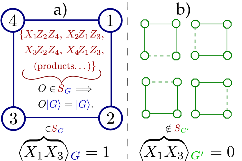
Figure 1: a) The square graph $G$. The associated state $\ket{G}$, as any graph state, possesses an associated structure of the stabilizer $S_{G}$ composed of specific strings of Pauli operators. Expectation values of any Pauli string $O$ is nonzero if and only if $\pm O\in S_{G}$. $X_{1}X_{3}$ is a stabilizer operator of $\ket{G}$ and therefore it’s expectation value is 1.
b) Graphs corresponding to the state defined in a) being altered by noise – here, the noise may remove certain edges (dashed lines). Noise processes change the stabilize group (e.g. by graph modification shown here), which allows for verifiable preparation.

In this section, we present a short introduction to the class of graph states and the stabilizer formalism. Readers familiar with the topic may skip directly to the next section.

A graph $G=(V,E)$ is defined by a set $V$ of vertices and a set of edges $E\subset V^{2}$: each $\{i,j\}=:e\in E$ denotes a connection between two vertices $i,j\in V$. Graph states are multi-qubit quantum states, where the vertices and edges of the graph $G=(V,E)$ represent qubits and entangling gates, respectively. The state $\ket{G}$, corresponding to a graph $G$ is defined as

$$\ket{G}=\mathchoice{}{}{}{}\prod_{\{i,j\}\in E}\mathchoice{}{}{}{}\operatorname{CZ}_{i,j}\ket{+}^{\otimes\lvert V\rvert},$$ (1)

where $\operatorname{CZ}$ denotes a standard controlled-$Z$ unitary operation

$$\operatorname{CZ}_{i,j}=\!\mathbbm{1}_{V\setminus\{i,j\}}\!\!\otimes\!\!\Big{(} \ket{00}\!\!\bra{00}\!+\!\ket{10}\!\!\bra{10}$$ (2)

$$\!\!+\!\ket{01}\!\!\bra{01}\!-\!\ket{11}\!\!\bra{11}\Big{)}_{i,j}.$$

Manifestly, all of controlled-$Z$ gates are diagonal in the computation basis, and hence commute – the product in the above equation does not depend on the order of operations.

Consider a four-vertex graph shown in Figure 1a: it has a vertex set $V=\{1,2,3,4\}$ and an edge set $E=\{\{1,2\},\{2,3\},\{3,4\},\{4,1\}\}$. The corresponding graph state is given by

$$\ket{G}=\operatorname{CZ}_{1,2}\operatorname{CZ}_{2,3}\operatorname{CZ}_{3,4}\operatorname{CZ}_{4,1}\ket{+}^{\otimes 4}.$$ (3)

The graph states can also be described using the so-called stabilizer operators, providing a description of the state in question in terms of its correlation structure. Consider an initial state $\ket{+}^{\otimes|V|}$: since it is a pure product state, there are no correlations between different sites. However, it is an eigenstate for each $X_{i}$ for $i\in V$. Let us denote the product of controlled-$Z$ operators in Equation 1 by $U$; then

$$\ket{G} =U\ket{+}^{\otimes\lvert V\rvert}=UX_{i}\ket{+}^{\otimes\lvert V\rvert}$$ (4)

$$=\underbrace{UX_{i}U^{\dagger}}_{g_{i}}\underbrace{U\ket{+}^{\otimes\lvert V\rvert}}_{\ket{G}}=g_{i}\ket{G}.$$ (5)

The operator $g_{i}$ can be shown to have the form of

$$g_{i}=X_{i}\mathchoice{}{}{}{}\prod_{j\in\operatorname{\mathcal{N}}(i)}\mathchoice{}{}{}{}Z_{j},$$ (6)

where $X_{i}$, $Y_{i}$, and $Z_{i}$ denote the Pauli matrices acting on the $i$-th qubit and $\operatorname{\mathcal{N}}(i)$ is the neighbourhood of $i$. As shown above, any graph state $\ket{G}$ defined by Equation 1 is an eigenstate (to the eigenvalue of $+1$) of all $g_{i}$:

$$g_{i}\ket{G}=\ket{G}$$ (7)

While the $(+1)$-eigenspace of each of the operators $g_{i}$ is highly degenerated, taken together they fully define the state $\ket{G}$: it is the $(+1)$-eigenstate of all $g_{i}$. Operators defined by Equation 7 commute; hence, they generate an Abelian subgroup of the group of Pauli operators, called the stabilizer $S$ of $\ket{G}$:

$$S=\left\{\prod_{i\in I}g_{i}:I\subset V\right\}.$$ (8)

The elements of the group $S$, due to the compact form of the generators (Equation 6), can be described with the help of low-dimensional matrices of integers modulo $2$ [21]. This representation is helpful in direct calculations involving the stabilizer.

The exemplary graph state shown in Figure 1a has stabilizer operators $g_{1}=X_{1}Z_{2}\operatorname{\mathds{1}}_{3}Z_{4}$, $g_{2}=Z_{1}X_{2}Z_{3}\operatorname{\mathds{1}}_{4}$, $g_{3}=\operatorname{\mathds{1}}_{1}Z_{2}X_{3}Z_{4}$, and $g_{4}=Z_{1}\operatorname{\mathds{1}}_{2}Z_{3}X_{4}$, as well as all products composed from these operators.

The elements of $S$ form a complete description of all possible correlations of local measurements of graph states: if a Pauli string $O=o_{i_{1}}o_{i_{2}}\ldots$ (or its negative, $-O$) appears in $S$, its expectation value on $\ket{G}$ is equal to $+1$ (respectively, $-1$), and if $\pm O\notin S$, $\langle O\rangle_{G}=0$.

For example, for the graph state shown in Figure 1a, the string $O=X_{1}X_{3}=g_{1}g_{3}$ is a stabilizer operator of $\ket{G}$. Using Equation 7 it can be seen that $\langle O\rangle_{G}=1$. The string $O^{\prime}=X_{1}Z_{3}\notin S_{G}$, hence $\langle O^{\prime}\rangle_{G}=0$. In this paper we are mostly using Pauli strings which contain only Pauli $X$ operators [21]. However, the results can be generalized to other Pauli strings.

The weighted graph states [22] are a related class of quantum states, for which controlled-phase operators are used instead of controlled-$Z$, with the phases possibly different for each edge of the graph $G$. If the phase associated with the edge $\{i,j\}$ is $\varphi_{i,j}$, the resulting state is defined by a modified version of Equation 1,

$${\ket{G_{\varphi}}=\mathchoice{}{}{}{}\prod_{\{i,j\}\in E}\mathchoice{}{}{}{}\operatorname{C\Phi}_{i,j}(\varphi_{i,j})\ket{+}^{\otimes\lvert V\rvert},}$$ (9)

where $\operatorname{C\Phi}(\varphi)=\operatorname{diag}(1,1,1,\exp(i\varphi))$ on the $\{i,j\}$ subsystem.S uch states arise naturally in systems with Ising-like interactions, and offer an useful representation of noisy graph state preparation using such a scheme. Unfortunately, the analogue of procedure described by Equation 5 does not produce a Pauli string, and hence a simple stabilizer description of correlations generally does not exist.

For a standard graph state $\ket{G}$ all phases $\varphi_{i,j}$ above are equal to $\pi$. This class of states naturally arises in systems with an Ising-type interaction pattern, and some physical realizations of graph states prepare the unweighted graph states in this exact way.

Many known families of states with structured entanglement can be represented as graph states. For instance, the $N$-qubit Greenberger–Horne–Zeilinger (GHZ) state [23], defined as

$$\ket{GHZ}=\frac{1}{\sqrt{2}}(\ket{0_{1}0_{2}\dots 0_{N}}+\ket{1_{1}1_{2}\dots 1_{N}})$$ (10)

is local unitary equivalent to the graph state of the fully connected $N$ vertex graph (or, equivalently, by the $N$ vertex star graph). In measurement-based quantum computing, cluster states, corresponding to grid graphs, are relevant [3], and intermediate-size cluster states have recently been realized on various platforms [24, 25]. A detailed discussion of graph states, including weighted graph states, can be found in [5, 26].

3 Correlations and measurement

It is possible to extract an entangled pair of qubits $(i,j)$ from a graph state $\ket{G}$ by means of local Pauli measurements, if there exists a path between $i$ and $j$ through the graph $G$ [20, 3]. In general, there are multiple ways to perform this task – and if noise is present, the entanglement quality of the resulting two-qubit state depends on the choice.

Consider a graph state $\ket{G}$ that undergoes a local sequential measurement process involving Pauli operators. The state of the unmeasured qubits is completely characterized by the measurement pattern along with the outcomes; the remaining correlations stem from the stabilizer operators of $\ket{G}$ consistent with the measurement pattern.

To see the structure of these correlations, let us choose a measurement pattern on a subset of qubits $I$: for each qubit $i\in I$, a local Pauli $o_{i}\in\{X_{i},Y_{i},Z_{i}\}$ is chosen. Then, each qubit $i$ is measured sequentially in the eigenbasis of the associated operator $o_{i}$. As mentioned previously, the expectation value of a Pauli string $O=\prod_{i\in I}o_{i}$ can be determined: if $O\in S_{G}$, it implies $\expectationvalue{O}_{G}=1$. The case of $-O\in S_{G}$ differs only by the sign, and if neither $\pm O\in S_{G}$, the expectation value is 0.

Let us concentrate on the positive sign case (the negative sign does not change much in reasoning) and consider an actual preparation of $\ket{G}$ and subsequent measurement according to $\{o_{i}\}_{i\in V}$: the measurement of $o_{i}$ on the $i$-th qubit has an outcome of $s_{i}$. If $\langle O\rangle_{G}=1$, the outcomes of the sequential measurement must reflect that: the signs of the measurement results must multiply to $+1$. Any other outcome pattern would decrease the magnitude of the experimental expectation value and is therefore incompatible with the graph state correlations.

This reasoning applies as well if the sequential measurement is stopped at any point and resumed afterward: if $O=\prod_{i\in I}o_{i}$ is a stabilizer, and only the qubits $I^{\prime}\subset I$ were measured, the sign structure of the further measurement of $I\setminus I^{\prime}$ can be predicted. Thus, by the action of partial measurement, correlation in the remaining qubits is induced.

The following Lemma captures this line of thought: the end correlations are defined by stabilizer operators consistent with the measurement scheme. Note that the measurement scheme does not itself have to be a stabilizer operator: only part of it has to extend to one, and this is always possible (see Lemma 3 in Appendix A).

Lemma 1.

Let $\ket{G}$ be a graph state determined by the graph $G=(V,E)$; we denote the stabilizer of $\ket{G}$ by $S$. If a subset $I$ of qubits is measured in such a way that a qubit $i\in I$ is measured in the eigenbasis of $o_{i}\in\{X_{i},Y_{i},Z_{i}\}$, we encode this measurement scheme as the Pauli string $O=\prod_{i\in I}o_{i}$. The qubits of $I$ are measured independently and sequentially, with the measurement outcome of $o_{i}$ denoted by $s_{i}=\pm 1$.

Let us now write a stabilizer operator $Q\in S$ of $\ket{G}$ as a Pauli string: $Q=\pm\prod_{j\in J}q_{j}$. The post-measurement state $\ket{\psi}$ is determined by those elements of the stabilizer, which are consistent with the measurement pattern $O$ such that $Q|_{I\cap J}=O|_{I\cap J}$. The stabilizer operators of the post-measurement state $\ket{\psi}$ can be computed from such operators $Q$ as

$$Q^{\prime}:=\pm\prod_{i\in I\cap J}s_{i}\prod_{j\in J\setminus I}q_{j}.$$ (11)

where the global sign is equal to the global sign of $Q$.

Proof.

Consider the stabilizer operator $Q$ defined as stated in the Lemma. Then assume that the measurement outcomes of each of the qubits $i\in I\cap J$ are $s_{i}$. Then, the projective measurement operators of these qubits can be written as $\frac{1}{2}\left(\mathbbm{1}_{i}+s_{i}q_{i}\right)$. Since the projection operators commute with $q_{j}$ themselves, the following chain of equalities holds:

$$\ket{\psi} =C\prod_{i\in I\cap J}\frac{\mathbbm{1}_{i}+s_{i}q_{i}}{2}\underbrace{\ket{G}}_{\leavevmode\nobreak\ \leavevmode\nobreak\ =Q\ket{G}}$$ (12)

$$=C\prod_{i\in I\cap J}\frac{\mathbbm{1}_{i}+s_{i}q_{i}}{2}\left(\pm\prod_{j\in J}q_{j}\ket{G}\right)$$

$$=\pm\prod_{j\in J\setminus I}q_{j}\prod_{i\in I\cap J}s_{i}\underbrace{\left(C\prod_{i\in I\cap J}\frac{\mathbbm{1}_{i}+s_{i}q_{i}}{2}\ket{G}\right)}_{\leavevmode\nobreak\ \leavevmode\nobreak\ =\ket{\psi}}$$

$$=\underbrace{\left(\pm\prod_{i\in I\cap J}s_{i}\prod_{j\in J\setminus I}q_{j}\right)}_{\leavevmode\nobreak\ \leavevmode\nobreak\ =Q^{\prime}}\ket{\psi}.$$

Here, $C$ is a normalization constant and the following equation (true for any $q$ such that $q^{2}=\mathbbm{1}$, in particular $q\in\{X,Y,Z\}$) was used:

$$\frac{\mathbbm{1}+sq}{2}q=s\frac{sq+\mathbbm{1}}{2}\quad\text{ for }s=\pm 1.$$ (13)

∎

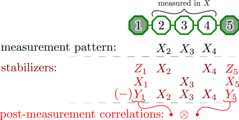
Figure 2: Partial local measurement of graph states induces correlations in the remaining qubits. Pictures is the path graph $5$ vertices: if the associated graph state is measured according to the shown measurement pattern, Bell-like correlations are induced in the two terminal qubits.

As an example, consider the line graph of 5 qubits, as shown in Figure 2 and the Pauli string $O=X_{2}X_{3}X_{4}$ which has support on vertices in $I=\{2,3,4\}$. The stabilizer set of the 5 qubit line graph contains $2^{5}$ stabilizers. Three of them are $Q^{(a)}=X_{1}X_{3}X_{5}$, $Q^{(b)}=Z_{1}X_{2}X_{4}Z_{5}$, and $Q^{(c)}=-Y_{1}X_{2}X_{3}X_{4}Y_{5}$ which have support on qubits in $J^{(a)}=\{1,3,5\}$, $J^{(b)}=\{1,2,4,5\}$, and $J^{(c)}=\{1,2,3,4,5\}$, respectively. It holds that $Q^{(a)}|_{3}=O|_{3}$, $Q^{(b)}|_{2,4}=O|_{2,4}$, and $Q^{(c)}|_{2,3,4}=O|_{2,3,4}$. Following Lemma 1, the post-measurement state after measuring qubits 2, 3, 4 in the $X$-basis is stabilized by $s_{3}X_{1}X_{5}$, $s_{2}s_{4}Z_{1}Z_{5}$, and $-s_{2}s_{3}s_{4}Y_{1}Y_{5}$. This can be viewed as a graph state (Bell pair) in a nonstandard basis – the change is an effect of the measurement performed on the qubits $\{2,3,4\}$.

The remaining qubits are fully defined by the correlations developed during the measurement process. Thus, it is possible to find measurement schemes for which the output state has certain properties: e.g., if the goal is to extract a Bell pair from a larger graph state $\ket{G}$, a measurement scheme $\prod_{i\in I}o_{i}$ must be found such that there exist stabilizers $Q$ of $\ket{G}$ such that $Q_{I\cup J}=O_{I\cup J}$ and ensuring Bell-like correlations between the terminal vertices. For example in the 5 qubit line graph and the above chosen measurements, the Bell state stabilizers are extracted; more elaborate measurement patterns have been studied for use in quantum networks [20, 19, 27]. Further examples for graph families analyzed later in this article can be found in Appendix A.

As a direct result of the Lemma 1 we get the following observation:

Corollary 1.

If a stabilizer operator $Q=\pm\prod_{j\in J}q_{j}$ is fully embedded in the measurement scheme $O=\prod_{i\in I}o_{i}$ such that $J\subset I$ and $Q=\pm O|_{J}$, the only observable sign structures within $J$ are those such that $\prod_{j\in J}s_{j}=\pm 1$, where the sign is determined by the sign in $Q$.

The proof follows by considering only $J\subset I$ in Lemma 1.

As mentioned in the introduction, the creation of a Bell pair is equivalent to the task of information transfer (teleportation) across the graph. This is so because if the Bell pair creation in the graph $G$ is viewed in the context of a larger graph $G^{\prime}$, this process (followed by measurement of one of the terminal qubits) performs qubit fusion: the unmeasured terminal qubit acts as the two combined. Since all local measurements with nonoverlapping supports do commute, this can be done before any other measurement or afterwards: in the latter case, the information created in one of the qubits is merged with the second one. This is captured by the following Lemma, represented pictorially by the Figure 3.

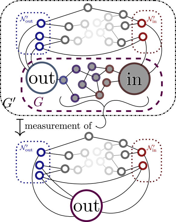
Figure 3: If a measurement scheme generates a Bell pair across the vertices $\{{\operatorname{in}},{\operatorname{out}}\}$ in the state corresponding to a graph $G$, in a larger $G^{\prime}$ it can be used to transfer information across the graph. Extending the measurement by a properly chosen operator $A_{{\operatorname{in}}}$ leads to the fusion of the two terminal vertices.

Lemma 2.

Consider a graph $G=\{V,E\}$, and choose the two terminal vertices $\{{\operatorname{in}},{\operatorname{out}}\}$ such that $V=\{{\operatorname{in}},{\operatorname{out}}\}\cup I$. Suppose that the corresponding graph state $\ket{G}$ undergoes a sequential measurement of $I$ producing a Bell pair across $\{{\operatorname{in}},{\operatorname{out}}\}$ in the meaning of Lemma 1.

With this determined, let us further assume that $G^{\prime}=(V^{\prime},E^{\prime})$ embeds $G$ in such a way that $\{{\operatorname{in}},{\operatorname{out}}\}$ is a separating set: the only connections between $G$ and the rest of $G^{\prime}$ are at these two vertices. Let us denote the vertices in $V^{\prime}\setminus V$ to which both qubits are connected by $\mathcal{N}^{\prime}({\operatorname{in}})$ and $\mathcal{N}^{\prime}({\operatorname{out}})$, respectively, and assume that the two sets are disjoint.

Within $G^{\prime}$, the aforementioned Bell pair-generating measurement followed by a product of single qubit unitary operations on the qubits $\{{\operatorname{in}},{\operatorname{out}}\}$ and the measurement $X_{\operatorname{in}}$ effectively performs qubit fusion of the terminal qubits. The new state is a graph state where the qubits $V^{\prime}\setminus V$ are intact, and the new neighborhood of the remaining qubit is $\mathcal{N}_{{\operatorname{out}}}\cup\mathcal{N}_{{\operatorname{in}}}$

Proof.

If within $G$ a Bell pair is produced across $\{{\operatorname{in}},{\operatorname{out}}\}$ as a result of the measurement pattern $O=\prod_{i\in L}o_{i}$ (where $L=V\setminus\{{\operatorname{in}},{\operatorname{out}}\}$), this means that there exist three $O$-consistent stabilizers involving the terminal vertices in the sense of Lemma 1. Combinatorical considerations show that one of those must be of a form such that the operators at the terminal vertices are $A_{\operatorname{in}},B_{\operatorname{out}}\in\{X,Y\}$ (but not $Z$), chosen independently.

Thus, there exists an $G$-stabilizer operator of the form $\pm A_{\operatorname{in}}B_{\operatorname{out}}\prod_{i\in I}o_{i}=g_{\operatorname{in}}g_{\operatorname{out}}\prod_{i\in I^{\prime}}g_{i}$, with $I,I^{\prime}\subset L$. Note that the definition of $g_{i}$ depends on the graph in question (Equation 6): if by $g^{\prime}_{i}$ we denote the generators corresponding to the entire graph $G^{\prime}$, the result is also a stabilizer, differing only by the $Z$ operators in the set $\mathcal{N}^{\prime}({\operatorname{in}})\cup\mathcal{N}^{\prime}({\operatorname{out}})$.

After the $A_{\operatorname{in}}$-basis measurement, we get a new stabilizer provided by Lemma 1:

$$\left(\pm s_{\operatorname{in}}\prod_{i\in L}s_{i}\right)B_{\operatorname{out}}\mathchoice{}{}{}{}\prod_{j\in\mathcal{N}^{\prime}_{\operatorname{in}}\cup\mathcal{N}^{\prime}_{\operatorname{out}}}\mathchoice{}{}{}{}Z_{j},$$ (14)

which can be taken to be a new stabilizer generator associated with the vertex ${\operatorname{out}}$, and brought to the canonical form of $X_{\operatorname{out}}\prod_{j\in\mathcal{N}^{\prime}_{\operatorname{in}}\cup\mathcal{N}^{\prime}_{\operatorname{out}}}Z_{j}$ by local unitary basis change of the ${\operatorname{out}}$-qubit. The properties of other stabilizers involving the qubits $\{{\operatorname{in}},{\operatorname{out}}\}$ can be proven similarly.

Thus, after the measurement within the Bell-generating part $L\cup\{{\operatorname{in}}\}$, the ${\operatorname{out}}$-qubit behaves exactly like it was connected to the neighborhood $\mathcal{N}^{\prime}_{\operatorname{in}}$ as well: the two vertices are fused and the information between them is transferred. ∎

4 Imperfect graph states

The reasoning presented above assumes that perfect $\operatorname{CZ}$ gates can be performed. However, this is not the case in experimental setups: some kind of noise is always present. In this section, we analyze three classes of physically motivated noise models; they all stem from different methods of graph state preparation. The origins and effects are sketched; for the detailed derivation, please refer to Appendix B.

Regardless of origin, noise processes often have a stabilizer-consistent description: vaguely speaking, they produce a mixture of stabilizer states, or the noise effect can be otherwise understood using the stabilizer-like correlations. In later sections, we show how to use this observation to mitigate the effects of noise.

4.1 Uncorrelated edge noise

Implementations like superconducting qubit quantum computers [28, 29], or ion traps [30, 31] prepare graph states by letting an initial product state evolve via an engineered Ising-like interaction Hamiltonian:

$$H=\sum_{i\neq j}\gamma_{i,j}\frac{(Z_{i}+\operatorname{\mathds{1}})\otimes(Z_{j}+\operatorname{\mathds{1}})}{4}.$$ (15)

Evolution according to such an interaction pattern effectively implements a sequence of controlled-phase operators $\operatorname{C\Phi}_{i,j}=\operatorname{diag}(1,1,1,\exp(-i\varphi_{i,j}))$. The structure of phases $\varphi_{i,j}=\gamma_{i,j}t$ is determined by the interaction strengths $\gamma_{i,j}$ and the evolution time $t$: inaccuracies in controlling either of them lead to the generation of a weighted graph state [22]. However, under general assumptions, the effective quantum channel implemented this way has a simple decomposition into local (one or two edges) operations, on top of the product of a sequence of $\operatorname{CZ}$ operations preparing the desired state.

Ideally, all of the generated phases $\varphi_{i,j}$ are equal to $\pi$. More realistically, with each experimental run, the actual realization will be $\varphi_{i,j}=\pi+\varepsilon_{i,j}$ with $\varepsilon_{i,j}\ll 1$. We discuss the two extremal cases of correlations of phase noises $\varepsilon_{i,j}$. The first, uncorrelated phase noise, assumes that the noises at different edges $(i,j)$ are completely independent. The other, correlated phase noise, assumes the contrary: each phase noise factor is equal to any other in a single experimental run, $\varepsilon_{i,j}=\varepsilon$. The noise encountered in experiments likely has yet a different structure with partial correlations between the edges; still, the two extremal processes may help in modeling the real-life scenario and strategies developed to mitigate them should apply in the more general cases.

Phases uncorrelated across the edges effectively lead to a probabilistic $\operatorname{CZ}$ (see the Appendix B) gate being implemented, if only each $\varepsilon_{i,j}$ is symmetrically distributed around $0$ (so that $\varphi=\pi+\varepsilon$ is centered around $\pi$). Each of controlled-$Z$ unitary operators in Equation 1 is replaced with the quantum channel

$$\operatorname{\mathcal{CZ}_{p}}[\rho]=(1-p)\operatorname{\mathcal{CZ}}[\rho]+p\rho,$$ (16)

where $p$ depends on the distribution of $\varepsilon$ and $\operatorname{\mathcal{CZ}}[\rho]=\operatorname{CZ}\rho\operatorname{CZ}^{\dagger}$.

Thus effectively the effect of noise is the generation of randomized graph states [32]: ensemble of graph states built atop the original graph $G$ by removing the edge $(i,j)\in E$ with probability $p_{i,j}$; related graph ensembles have been introduced in [33] in a classical context. For the constant probability, the end state can be written as

$$\rho=\sum_{E^{\prime}\subset E}(1-p)^{|E^{\prime}|}p^{|E\setminus E^{\prime}|}\ket{G^{\prime}}\bra{G^{\prime}},$$ (17)

where $G^{\prime}=(V,E^{\prime})$ is a graph with edge set $E^{\prime}$ being a subset of the edge set $E$ of the original graph $G$.

Note that it is an effective description: in each experimental run, the prepared state is a pure weighted graph state [13]; the density operator in Equation 17 is a state of knowledge about the system, averaged over different noise realizations.

4.2 Correlated edge noise

If the weights in the Hamiltonian of Equation 15 are perfect ($\gamma_{i,j}=1$) but the interaction time is not perfectly controlled, within one experimental run, all the resulting phases $\varphi_{i,j}$ are equal. This is correlated phase noise: it has an effect similar, but more involved, to the uncorrelated case. Here, we also assume that $\varphi$ is symmetrically distributed around $\pi$. Let us assume that in each experimental run $\varphi_{i,j}=\varphi=\pi+\varepsilon$, and $\varepsilon$ is distributed with the normal distribution of the standard deviation $\sigma$. Then, with $p$ depending on the phase distribution (see Appendix B for details), the lowest order of approximation of the state (essentially, keeping only terms of order $\varepsilon^{2}$ in the end state and subsequent averaging) can be described with the help of square roots of the unitary operator $\operatorname{CZ}$:

$$\rho= (1-p\lvert E\rvert)\ket{G}\bra{G}+p\sum_{e\in E}\outerproduct{G-e}{G-e}$$ (18)

$$+p\!\!\!\!\sum_{\{e,e^{\prime}\}\subset E\leavevmode\nobreak\ \leavevmode\nobreak\ \leavevmode\nobreak\ \phantom{x}}^{e\neq e^{\prime}}\!\!\!\!\!\!\!\!\!\!\!\!\!\sum_{\phantom{x}\leavevmode\nobreak\ \leavevmode\nobreak\ \pm_{1},\pm_{2}}\!\!\!\!\!\!\!\pm_{1}\!\pm_{2}\!{\operatorname{\mathcal{CS}}_{e}^{\pm_{1}}}\!\!{\operatorname{\mathcal{CS}}_{e^{\prime}}^{\pm_{2}}}[\ket{G}\bra{G}].$$

Note that this decomposition is not convex and cannot be interpreted as an ensemble: the minus signs in front of the decomposition terms prevent this. Signs appear as a result of discrete decomposition of controlled-phase and subsequent averaging; see Appendix B for details. In this decomposition, $G-e\coloneqq(V,E\setminus\{e\})$ is the graph with edge removed, and ${\operatorname{\mathcal{CS}}^{\pm}}$ is the application of one of the two unitary square roots of $\operatorname{CZ}$:

$${\operatorname{\mathcal{CS}}^{\pm}}[\rho]=\sqrt{\operatorname{CZ}^{\pm}}\rho\sqrt{\operatorname{CZ}^{\pm}}^{\dagger},$$ (19)

where

$$\sqrt{\operatorname{CZ}^{\pm}}\coloneqq\frac{1}{2}\left[\left(1+e^{\pm i\frac{\pi}{2}}\right)\operatorname{\mathds{1}}+\left(1-e^{\pm i\frac{\pi}{2}}\right)\operatorname{CZ}\right].$$ (20)

4.3 Local $Z$ flip noise

In linear optic experiments, where Bell pairs are generated and subsequently fused to get a graph state, the entangling operation may fail as a result of partial photon distinguishability (by imperfect frequency of spatial mode overlap) [34, 35, 36] – for a derivation see the Appendix B. The effect of a noisy fusion gate described this way can be modeled as a perfect fusion followed by a probabilistic application of the $Z$ unitary to the surviving optical qubit $i$:

$$F_{i}(\rho)=(1-p)\rho+pZ_{i}\rho Z_{i}.$$ (21)

Here, the probability $p$ depends on the level of photon distinguishability of the fused qubits. Thus, the final graph state developed in this procedure can be thought of as a probabilistic application of local $Z$ unitaries to each of the qubits in the graph.

4.4 Quantification of the noise effects

In the following chapters, we determine the entanglement quality of a small (two- or three-qubit) subsystem left after a measurement procedure performed on a graph state: this is the Bell pair or GHZ state extraction, since ideally the resulting state would represent correlations found in these states. We have chosen fidelity with respect to the ideal state as a measure of the entanglement quality. In the absence of noise, the initial state $\ket{G}$ is pure, and measurement of an $i$-th qubit in the basis of an operator $o_{i}\in\{X_{i},Y_{i},Z_{i}\}$ leads to observation of an outcome $\pm 1$. On the algebraic level, this corresponds to application of an operator $\frac{1}{2}\left(\mathbbm{1}\pm o_{i}\right)$ to the pre-measurement state, and after the entire procedure, the post-measurement state $\ket{\psi}$ is still pure. This allows a simple determination of the fidelity with respect to the noisy state $\rho$: if the post-measurement state is $\sigma$, the following holds.

$$\mathcal{F}(\ket{\psi}\!\bra{\psi},\sigma)=\langle\psi|\sigma|\psi\rangle.$$ (22)

Note that the ideal post-measurement state depends on the observed outcomes during the experiment: they do affect the signs in the final stabilizer structure (see Lemma 1). Therefore, the ideal state $\ket{\psi}$ must be determined from the signs of the outcomes. This is only possible if the structure is consistent with the stabilizers of the ideal state; this is not an issue, since we explicitly postselect on the right set of outcomes in the following sections as part of the error mitigation strategy. Finally, the average fidelity $\langle\mathcal{F}\rangle$ is determined for all possible measurement outcomes consistent with the stabilizer structure; this is effectively approximated by taking $N$ samples from the defining ensembles for a specific noise model with a Monte Carlo algorithm and thus

$$\langle\mathcal{F}\rangle=\frac{1}{N}\!\!\!\sum_{\text{outcomes}}\!\!\!\mathcal{F}(\text{outcome}).$$ (23)

Since we are mostly interested in the behavior in the low noise limit, we define fidelity susceptibility $\alpha$ as the rate of change of mean fidelity $\langle\mathcal{F}\rangle(p)$: the ensemble of extracted and postselected states depends on the noise, and the susceptibility captures the effects of small but not negligible noise.

$$\alpha=-\left.\frac{\differential\langle F\rangle(p)}{\differential p}\right|_{p=0}.$$ (24)

For zero noise, the fidelity is equal to 1 by definition. For any other amount, the fidelity may only decrease, and hence the susceptibility is positive. Its numerical magnitude determines how fragile the extraction procedure is to the effects of noise: a robust one has a small (or, in some cases, even zero) susceptibility.

5 Extraction from noisy ensembles

In this section we apply the methods developed in previous parts to show the effects of the noise and find measurement patterns that minimize them. Instead of focusing on teleportation directly, we analyze the (equivalent) task of extracting a high-quality Bell pair from a larger noisy state, close to a graph state $\ket{G}$.

5.1 Noise-correcting structures and robust families of states

As introduced above, noise processes lead to an ensemble of different states $\{(p_{i},\ket{\psi_{i}}\}$ being prepared, where one of the ensemble components is the ideal state $\ket{G}$. This ensemble can be interpreted as a probabilistic preparation of an unknown state $\ket{\psi_{i}}$ with probability $p_{i}$. The same measurement procedure as previously might now yield results inconsistent with $\ket{G}$, and observations of those are an indication of state other than $\ket{G}$ being prepared.

As an example, consider the graph $G$ to be a $4$-cycle of vertices $\{1,2,3,4\}$, as shown in Figure 1a. The operator $O=X_{1}X_{3}$ belongs to a stabilizer of $\ket{G}$, thus the only sign structures that can be observed in the sequential measurement of qubits $1$ and $3$ are $+1,+1$ and $-1,-1$. Consider now all edge subgraphs $\{G^{\prime}\}$ of $G$ and a physical process in which an ensemble of graph states $\{p_{G^{\prime}},\ket{G^{\prime}}\}$ is prepared, some of them are shown in Figure 1b. The operator $O$ (and $-O$) is not a part of the stabilizer of any proper subgraph with at least one edge; thus, sign structures of $+1,-1$ or $-1,+1$ are possible: observing those in the same measurement procedure implies that the pre-measurement state was not $\ket{G}$.

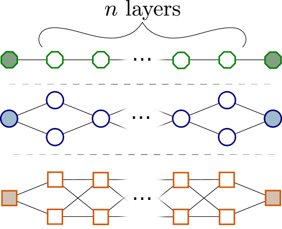
Figure 4: Considered families of graphs for the task of Bell pair extraction, parameterized by the length of the internal part $n$. The terminal qubits, designated for creation of a Bell pair, are denotes with filled nodes. From the top: path graph, twisted pair, crazy graph.

The postselection on the right measurement outcomes consistent thus performs a probabilistic check whether $\ket{G}$ was truly prepared. However, the existence of such parity-checking structures depends on the graph and the task for which the associated quantum state is used.

A Bell pair can be prepared with the help of a path graph state and local $X$ measurements, but such a system does not support embedded stabilizer operators. Other graphs and measurement patterns do better in this regard, and here we present them. The families of graph states analyzed are parameterized by the length between the terminal qubits across which a Bell pair is to be prepared (see Figure 4). Apart from a simple path graph, included as a benchmark for comparison, we include two other families described below – both of them have their strengths.

The twisted pair graph [37] is built from layers, where each qubit in the layer $k$ is connected with every qubit from the layers $k-1$ and $k+1)$. The number of qubits in each layer alternates between $1$ and $2$, which enables the existence of a restricted set of stabilizers: for each 2-qubit layer consisting of the qubits $\{i,j\}$, the operators $X_{i}X_{j}$ stabilize $\ket{G}$. Additionally, it is very robust to certain types of noise, because of its relatively simple geometry.

The crazy graph (studied in [38, 14] for its noise robustness) also consists of layers of $2$ qubits each, with a similar full connectivity structure between the adjacent layers. This ensures a robust and simple to analyze structure of the embedded stabilizer operators (see Appendix A and Figure 5).

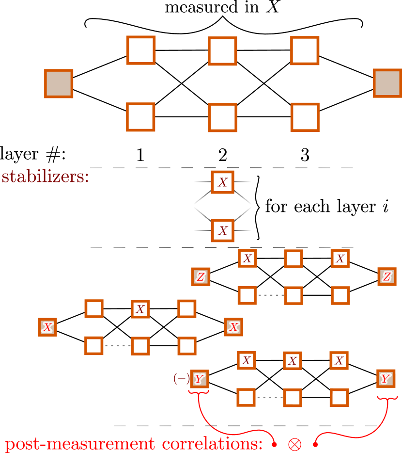
Figure 5: Crazy graph of length 3 together with an all-$X$ measurement pattern possess embedded error-checking and correction structures. Middle: each layer is associated with an $X\otimes X$ stabilizer, which can be used to confirm the proper preparation of the state. Bottom: even if any single internal edge (dotted line between layers 1 and 2) is missing, the terminal qubits correlations are not affected: the operators shown are stabilizers, regardless of whether the edge is present or not.

Both presented structures generalize to the extraction of other types of states, in which context they serve as a direct replacement of path graphs. We mention the usage in a task of 3-qubit GHZ state extraction.

5.2 Bell pair quality scaling for different type of noise

Each of the graph states associated with the aforementioned three families (path graph, twist graph, and crazy graph) can be used for extraction of a Bell pair across the terminal qubits. Only local $X$ measurements are used for all three, and the fact that in the ideal case a maximally entangled state is produced is captured by the stabilizer operators consistent with this measurement pattern.

As a simple example, consider the 5 qubit line graph as discussed in Section 3. Measurements in the $X$ basis on all but the terminal qubits lead to a two-qubit state which can be shown to have Bell-like correlations. Similar structures can be found for all the three graph families mentioned: sets of stabilizer operators ensuring correlations of the terminal qubits, having only $X$ operators in the internal section (and thus compatible with the measurement scheme).

The effect of noise destroys the perfect correlations: even if for every ensemble element the end state is maximally entangled, the mixture of such states might have less (or none) entanglement. Postselection on the measurement outcomes consistent with the ideal stabilizer structure helps twofold: one of its effects is probabilistic error detection. The other, appearing in the case of the crazy graph ensemble, is more subtle: after postselection, the end state may be the same for a large portion of the ensemble elements (see Appendix A).

The results, presented in Figure 6, show that this approach (noise-detecting structures combined with postselection) works for different types of noise. The fidelity susceptibility (quantifying the initial fidelity falloff in the low noise limit; see Equation 24) is reduced for the twisted pair and crazy structures. Furthermore, the susceptibility for the crazy graph structure does not depend on the length, as a result of the correctional stabilizers mentioned in the previous paragraph. This behavior is observed both for uncorrelated phase noise, resulting in probabilistic edge losses and a local $Z$ flip noise.

An additional entanglement-preserving structure can be found in the case of perfectly correlated phase noise. The authors of Ref. [13] recently observed that in the case of the path graph, postselection on different measurement outcomes yields vastly different results in the terms of entanglement quality; we have found that this result does generalize to the other linear graphs analyzed by us. Both for the crazy and double twist graph families the lowest order nontrivial noise effects can be canceled completely if all the measurement outcomes are postselected on measuring the minus outcome of $X$. This is consistent with our previous observations: such an observed measurement pattern does not violate parity constraints arising from the stabilizer structure. This result can be understood by studying the modifications of the stabilizer operators of $\ket{G}$ under correlated controlled-phase noise.

For the square graph presented in Figure 1a, if instead of the perfect controlled-$Z$ unitary, the $\operatorname{C\Phi}(\pi+\varepsilon)=\operatorname{diag}(1,1,1,-1\exp(i\varepsilon))$ is used (so that $\operatorname{C\Phi}=\operatorname{CZ}$ for $\varepsilon=0$), the four-qubit entangled state is a weighted graph state $\ket{G}_{\varepsilon}$. If qubits 1 and 3 are measured in the $X$ basis, we expect the measurement outcomes to be equal (we exclude the cases when it does not hold). With the weighted graph state $\ket{G}_{\varepsilon}$ as the initial state, let us denote the unnormalized post-measurement state by

$$\ket{X_{1,3}\pm}=\frac{\mathbbm{1}\pm X_{1}}{2}\frac{\mathbbm{1}\pm X_{3}}{2}\ket{G}_{\varepsilon}.$$ (25)

The relevant expectation values defining the end correlations (with $\langle O\rangle_{\pm}$ denoting the expectation value of $O$ for the unnormalized state $\ket{X_{1,3}\pm}$) across qubits $2$ and $4$ are the following, in the lowest nontrivial noise order:

$$\langle Z_{2}Z_{4}\rangle_{+} =1-\varepsilon^{2}, \langle Z_{2}Z_{4}\rangle_{-} =-1+\frac{\varepsilon^{2}}{2},$$ (26)

$$\langle X_{2}X_{4}\rangle_{+} =1-3\varepsilon^{2}, \langle X_{2}X_{4}\rangle_{-} =-1+\frac{\varepsilon^{2}}{2},$$

$$\langle Y_{2}Y_{4}\rangle_{+} =-1+3\varepsilon^{2}, \langle Y_{2}Y_{4}\rangle_{-} =1+\frac{\varepsilon^{2}}{2},$$

$$\||X_{1,3}+\rangle\|^{2} =1-\varepsilon^{2}, \||X_{1,3}-\rangle\|^{2} =1-\frac{\varepsilon^{2}}{2}.$$

Note that for the $\ket{X_{1,3}-}$ outcome the squared length $\||X_{1,3}-\rangle\|^{2}$ is proportional to the unnormalized expectation values: thus, for the physical correlations the dominant noise effects are canceled and only higher order terms ($O(\varepsilon^{4})$) remain. On the other hand, if the outcome is $\ket{X_{1,3}+}$, the noise is amplified compared to postselection on only stabilizer-consistent outcomes. Thus, further postselection can amplify the entanglement quality of the remaining qubits at the cost of discarding certain outcomes and reduced production rates.

The double twist graph can be viewed as multiple such squares stacked together by the terminal vertices: thus, a proper postselection can mitigate the first nontrivial noise effects completely (see Figure 7). A similar structure appears for the crazy graph: it is much more complex to analyze it, but computer algebra systems provide evidence of a periodic structure of susceptibilities as the length of the graph increases.

Figure 6: Susceptibility of the Bell pair entanglement quality to edge loss (top) and local phase flip (bottom) noise. Pictured is the linear part of concurrence decrease for the three analyzed families (with postselection on the measurement outcomes consistent with the ideal state) in the low noise limit, where the dominant contributions are the single edge losses (top) and single qubit flips (bottom). The constant susceptibility of the crazy graph is a result of the noise at the terminal edges only: each internal edge loss is automatically corrected for and every single flipped qubit is detected.

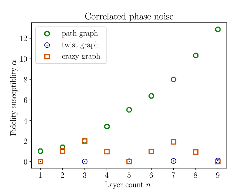
Figure 7: Susceptibility of the Bell pair entanglement quality for correlated phase noise. Here, only the cases postselected on observing exclusively minus signs during the $X$ measurement are taken into account. In this regime, the twist graph is able to remove the effect of noise completely (in the lowest nontrivial orders), and the crazy graph shows a periodic pattern of susceptibilities, still significantly reducing the noise effect. The situation inverts for observing exclusively $+$ signs: then, the noise gets amplified.

6 Extraction of GHZ states

The methodology applied for Bell pair extraction generalizes to the extraction of GHZ states [23]: generally, for $N$ qubits, they correspond to a star graph with a central qubit connected to the remaining $N-1$ ones (or, equivalently, a complete graph of $N$ qubits). Here, we concentrate on the case $N=3$ and adopt star-shaped graph structures built from the graph patterns used in Bell pair creation. Refer to Figure 8a for an illustration of the structure: it is built on the template of several crazy graphs, stitched at the central pair of vertices. The fidelity response, presented in Figure 8b, is more resilient to noise (as compared to the simpler path graph) also in this new task of extraction of the GHZ state.

The data presented in this figure require calculations involving a large number of ensemble states and measurement outcomes. To mitigate the numerical difficulty, a Monte Carlo method was utilized. The figure of merit – fidelity – is linear with respect to the ensemble- and measurement outcome averaging, provided the target state is pure. Thus, this approach allows for an approximation of fidelity by sampling ensemble elements and measurement outcomes, avoiding direct calculations with density operators. The fidelity of the output state to the ideal pure state is estimated using this method until the plots converge smoothly and the variance of the fidelity estimator is negligible.

Analysis of the data in Figure 8 shows that the fidelity response for both the GHZ and Bell state extractions exhibits qualitatively similar behavior: most importantly, the susceptibility is greatly reduced in the low noise limit. Thus, the ’crazy graph’ structures can generalize beyond Bell pair extraction to more complex multi-qubit systems, maintaining their noise-resilient properties. This performance gain is due to the noise-detecting and -correcting capabilities intrinsic to these graph families. Further investigations of different connectivity structures suggest that this behavior is universal, although a formal proof is beyond the scope of this study. If true, the ’crazy graph’ can serve as a link similar to a simple path link, similar in function but implementing some level of error correction.

a)
b)

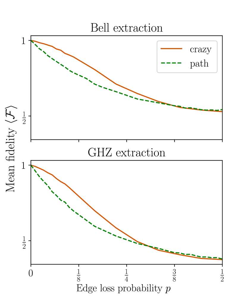
Figure 8: a) Structures of the analyzed graphs analyzed: path and crazy templates yielding Bell pairs and 3-qubit GHZ states upon measurements of the central qubits. b) Fidelity of the end state with respect to the ideal Bell and GHZ states as a function of noise. The fidelity is averaged over possible measurement outcomes consistent with the measurement-embedded stabilizer structures. The initial fall-off rate of fidelity at $p=0$ is the fidelity susceptibility, defined in Equation 24.

7 Summary and Outlook

This study has advanced the understanding of noise processes in graph states, specifically addressing the effects of preparation by the Ising-like interaction and photonic qubit fusion. We have found graph structures applicable in error detection and correction, especially in tasks such as information transfer and GHZ state preparation. This approach uses additional qubits for probabilistic verification and demonstrates a new method to improve resilience against specific noise disturbances.

Future research may include more general tasks found in the measurement-based quantum computation approach. So far, our results are applicable to measurement patterns composed of Pauli operators, but it is known to restrict the set of possible operations to a clasically simulable one: a similar method, based on non-Pauli measurements, but still allowing for noise effects reduction, could open new pathways for quantum computation, albeit with conceptual and practical complexities. The methods presented here can be generalized for arbitrary output graph geometry, and the applicability of this procedure for quantum metrology [39] could be studied.

Additional platforms for generating graph states can also be analyzed: in this context, sequential single-atom emitters [25] are especially interesting. Although noise processes are fairly complex, such systems are capable of producing extensive path graph states and present a unique opportunity for advancing graph state generation techniques. Different experimental realizations natively support different connectivity structures [24, 25, 30, 40, 41], and optimal utilization of a given experimental setting may require further development of the presented techniques.

To summarize, this research contributes new insights into noise reduction in graph state-based systems, implications of which include applications of measurement-based quantum computation. We hope to apply a similar approach for different applications and determine its utility as graph states are realized on existing quantum devices.

Appendix A Post-measurement correlations and stabilizers compatible with the measurement scheme

Lemma 3.

Given a graph state $\ket{G}$ of $N$ qubits and a certain measurement scheme defined in Lemma 1 by a set of qubits $I$ and operators $o_{i}$, then the subset of the stabilizer of $\ket{G}$ compatible with the measurement pattern has $N-\lvert I\rvert$ generators, and therefore fully defines the post-measurement state.

Proof.

The stabilizer of $\ket{G}$, up to the structure of the signs, can be viewed as a linear subspace of $\mathbb{Z}_{2}^{2N}$ – this is known as the binary representation of the stabilizer [5]. The identification is following: if the stabilizer operator is defined as $\prod_{j\in J}g_{j}$, the corresponding element of $\mathbb{Z}_{2}^{2N}$ is $(x_{1},\ldots,x_{N})\oplus(z_{1},\ldots,z_{N})$, with $x_{i}$ being 1 if and only if $i\in J$ and $\vec{z}=A_{G}\vec{x}\mod 2$, where $A_{G}$ is the adjacency matrix of $G$. Thus, if a stabilizer contains $X_{i}$, the corresponding numbers are $(x_{i},z_{i})=(1,0)$, for $Z_{i}$ it is $(x_{i},z_{i})=(0,1)$, and $Y_{i}$ corresponds to $(x_{i},z_{i})=(1,1)$; no operator at site $i$ is denoted by $(x_{i},z_{i})=(0,0)$. In this way, the additive algebra of $\mathbb{Z}_{2}^{2}$ mimics the product rules of Pauli operators with only the missing sign structure.

The stabilizer of $\ket{G}$ corresponds to a special $N$-dimensional subspace in $\mathbb{Z}_{2}^{2N}$ [5]. For any stabilizer operator to be compatible with the measurement scheme in the sense of Lemma 1, each operator of its Pauli string form with support in $I$ must be $o_{i}$: this introduces constraints to the set of compatible operators. However, these constraints translated into the language of $\mathbb{Z}_{2}^{2N}$ are linear: if $X_{i}$ is measured at site $i$, the additional constraint is $z_{i}=0$ (this encompasses the cases of $X_{i}$ and identity at site $i$), if $Z_{i}$ is measured, the constraint is $x_{i}=0$, and for $Y_{i}$ it is $x_{i}+z_{i}=0\mod 2$. All of them are independent, and there are $\lvert I\rvert$ of them, one for each measured site. Thus, the linear subspace of $\mathbb{Z}_{2}^{2N}$ corresponding to measurement-compatible stabilizers has dimension $N-\lvert I\rvert$; any basis of this subspace corresponds to generators of the post-measurement state stabilizer. ∎

For example, the correlations that stem from the measurement described after Lemma 1 and in Figure 2 correspond to the following $\vec{x}\oplus\vec{z}$ vectors in the binary representation:

$$(0,1,0,1,0) \oplus(1,0,0,0,1),$$ (27)

$$(1,0,1,0,1) \oplus(0,0,0,0,0),$$

$$(1,1,1,1,1) \oplus(1,0,0,0,1).$$

The third vector is a linear combination of the first two; thus the space of end correlations is two-dimensional.

A.1 Patterns for specific graph families

Consider a path graph $G$ of $n+2$ vertices $V=\{0,1,\ldots,n,n+1\}$ with edges $E=\{\{k,k+1\}\}_{k=0}^{n}$. If the qubits $\{1,\ldots,n\}$ of the associated state $\ket{G}$ are measured in the basis of $X$, this induces correlations in the remaining unmeasured qubits $0$ and $n+1$. This follows from the fact that the following stabilizer operators are consistent with the measurement pattern:

$$Z_{0}Z_{n+1}\prod_{k\in I}X_{k}, \leavevmode\nobreak\ \leavevmode\nobreak\ \leavevmode\nobreak\ X_{0}X_{n+1}\prod_{k\in I^{\prime}}X_{k}, (\text{odd }n)$$ (28)

$$Z_{0}X_{n+1}\prod_{k\in I}X_{k}, \leavevmode\nobreak\ \leavevmode\nobreak\ \leavevmode\nobreak\ X_{0}Z_{n+1}\prod_{k\in I^{\prime}}X_{k}. (\text{even }n)$$

where $I$ ($I^{\prime}$) is the set of odd (even) numbers between $1$ and $n$:

$$I =\{k\in\{1,2,\ldots,n\}:k=1\mod 2\},$$ (29)

$$I^{\prime} =\{k\in\{1,2,\ldots,n\}:k=0\mod 2\}.$$

.

Thus, if the outcome of the $X_{k}$ measurement is denoted by $s_{k}$, the following operators generate the post-measurement stabilizer of the terminal qubits $\{0,n+1\}$:

$$Z_{0}Z_{n+1}\prod_{k\in I}s_{k}, \leavevmode\nobreak\ X_{0}X_{n+1}\prod_{k\in I^{\prime}}s_{k}, (\text{odd }n)$$ (30)

$$Z_{0}X_{n+1}\prod_{k\in I}s_{k}, \leavevmode\nobreak\ X_{0}Z_{n+1}\prod_{k\in I^{\prime}}s_{k}. (\text{even }n)$$

Both cases are consistent with a maximally entangled two-qubit state being produced in the terminal qubits: for the odd-$n$ case, the existence of stabilizers described by LABEL:eqn:termoddpathcorr ensures that further measurement of $X$, $Y$ or $Z$ at qubit $0$ is perfectly (anti)correlated with the outcome of measurement of the same operator at qubit $n+1$.

This result generalizes to the case where each qubit $k$ is replaced by a set of $m_{k}$ qubits in such a way that the adjacent layers are fully connected. In this case, the qubits are denoted by pairs of numbers $(k,i)$, where $k=\{0,1,\ldots,n,n+1\}$ is the layer index and $i\in\{1,\ldots,m_{k}\}$ is the qubit index within the layer. The edges exist between any layer-adjacent qubit:

$$E=\{\{(k,i),(k+1,j)\}:k\in\{0,\ldots,n\},i\in\{1,\ldots,m_{k}\},j\in\{1,\ldots,m_{k+1}\}\}.$$ (31)

This class of graphs includes the path graph (each layer has only a single qubit), the crazy graph (the layers $0$ and $n+1$ contain one qubit each, every other has two) and twisted graphs (the qubit count alternates between 1 and 2) as well. Suppose that all the internal qubits in every layer are measured in the $X$ basis. The stabilizer operators that determine the remaining correlations must be consistent with this structure. A particularly simple set of such operators exists: first, observe that if a layer $k$ contains at least two qubits, $X_{k,i}X_{k,i^{\prime}}$ is a stabilizer operator. Thus, the signs of outcomes have to be equal within a layer. Therefore, for any choice of inner-layer qubit index $(i_{k})$ the direct analogue of LABEL:eqn:stabextended holds:

$$Z_{0}Z_{n+1}\prod_{k\in I}X_{k,i_{k}}, \leavevmode\nobreak\ X_{0}X_{n+1}\prod_{k\in I^{\prime}}X_{k,i_{k}}, (\text{odd }n),$$ (32)

$$Z_{0}X_{n+1}\prod_{k\in I}X_{k,i_{k}}, \leavevmode\nobreak\ X_{0}Z_{n+1}\prod_{k\in I^{\prime}}X_{k,i_{k}}, (\text{even }n),$$

are stabilizer operators. For symmetry, we assume the twisted graph structure exists only for an odd number of layers, so that the terminal ones consist only of one qubit each. Thus, the terminal layers $0$ and $n+1$ always consist only of one qubit each, and the inner indices are omitted. Consequently, if $s_{k}$ in LABEL:eqn:termoddpathcorr are interpreted as signs of outcomes at layer $k$ (which are all equal within a layer due to the structure of the stabilizer operators mentioned previously), the same post-measurement stabilizer structure appears.

In the case of the crazy graph, an additional observation can be made: loss of any single internal (not adjacent to the terminal qubits) edge yields the same post-measurement stabilizer structure, since the indices $(i_{k})$ in LABEL:eqn:stabextendedgeneral can be chosen arbitrarily. Thus, the crazy graph family is especially tolerant to single edge loss: it does not affect the post-measurement state, if the outcomes are postselected on the ideal sign structure. This can be generalized to the loss of any subset of edges not adjacent to each other and the terminal qubits.

Appendix B Derivation for the noise models

B.1 Uncorrelated phase noise

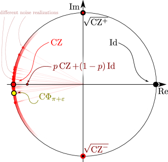
Figure 9: The controlled-$Z$ gate, if implemented as controlled phase operation, is susceptible to phase variations. In each experimental run the phase is constant, and the resulting state is a weighted graph state. Since this phase is unknown, the effective quantum state is weighted graph state, averaged over different noise realization. For just a single edge, if the phase distribution is centered around $\pi$ (corresponding to the ideal graph state), the resulting quantum channel is a mixture of controlled-$Z$ and identity: the edge is probabilistically generated.

In certain ion traps and superconducting quantum devices, the sequence of $\operatorname{CZ}$ gates is realized with evolution with an Ising-type Hamiltonian:

$$H=\sum_{(i,j)\in G}\gamma_{i,j}\frac{Z_{i}+1}{2}\frac{Z_{j}+1}{2}.$$ (33)

For constant $\gamma=\gamma_{i,j}$, the unitary operation $\exp(-iHt)$ exactly corresponds to the product of $\operatorname{CZ}$ gates appearing in Equation 1 for $t=\frac{\pi}{\gamma}$. However, incomplete control over the system leads to a fluctuation of the interaction strengths $\gamma_{i,j}$. In such case, each of the two-body terms appearing in Equation 33 gives rise to a controlled phase operation $\operatorname{C\Phi}_{i,j}=\operatorname{diag}(1,1,1,\exp(-it\gamma_{i,j}))$ in the appropriate two-body subsystem. The quantum channel corresponding to this gate decomposes:

$$\operatorname{C\Phi}\rho\operatorname{C\Phi}^{\dagger}=\frac{1-\cos\phi}{2}\operatorname{\mathcal{CZ}}[\rho]+\frac{1+\cos\phi}{2}\rho+\frac{\sin\phi}{2}\operatorname{\mathcal{CS}}^{+}[\rho]-\frac{\sin\phi}{2}\operatorname{\mathcal{CS}}^{-}[\rho],$$ (34)

where $\phi=t\gamma_{e}$ and $\operatorname{\mathcal{CS}}^{\pm}$ is defined in Equation 19. If the actually realized phase cannot be measured classically in each experimental run, the resulting state is a mixture of states:

$$\rho=\int P(\{\gamma_{i,j}\})\ket{G_{\gamma}}\bra{G_{\gamma}}\differential\gamma,$$ (35)

where $P(\{\gamma_{e}\})$ denotes the probability distribution of phases and $\ket{G_{\gamma}}=\left(\prod_{i,j}\operatorname{C\Phi}_{i,j}\right)\ket{+}^{\otimes N}$. If the strength noise is independent for each edge (i.e. $P=\prod P_{e}$) and symmetric around $\pi$, a significantly easier description of the state $\rho$ can be found: each controlled-phase averages to a mixture of controlled-$Z$ and identity (see Figure 9), since these are the only terms appearing in Equation 34 with prefactors symmetric around $\pi$. Thus, noise effectively leads to the generation of randomized graph states: this is an ensemble of graph states, where the edge $e\in E$ is missing with probability $p_{e}$:

$$\rho=\sum_{E^{\prime}\subset E}\left(\prod_{{\{i^{\prime},j^{\prime}\}\in E^{\prime}}}\!\!\!(1-p_{i^{\prime},j^{\prime}})\!\!\!\prod_{\{i,j\}\notin E^{\prime}}\!\!\!p_{i,j}\right)\ket{G^{\prime}}\bra{G^{\prime}},$$ (36)

where the graph $G^{\prime}$ has the edges defined by the set $E^{\prime}$. The probability $p_{i,j}$ can be determined by the statistical properties of the distribution of the phase $\phi$ associated with the edge $\{i,j\}$. In particular, for the normal distribution of $\varepsilon$ centered around $\pi$ with the standard deviation of $\sigma$ the probability $p$ takes the closed form of

$$p=\frac{1-\exp\left(-\frac{\sigma^{2}}{2}\right)}{2}=\frac{\sigma^{2}}{4}-\frac{\sigma^{4}}{16}+O(\sigma^{6}).$$ (37)

B.2 Correlated phase noise

Correlated phase noise has similar, but more involved effect. Suppose that the weights in Hamiltonian Equation 33 are all the same, but the interaction time varies. In such a case, the phase is the same for each controlled-phase operator, and the decomposition used to derive Equation 17 breaks. This is due to the fact that in the integrand of Equation 35 there exist additional terms symmetric around the ideal phase of $\phi=\pi$. There are the terms proportional to $\sin\phi$ in Equation 34: even powers of them also contribute to the final state. Thus, in the lowest order or approximation the output state is described by:

• The unmodified state graph state $\ket{G}$ with reduced probability coming from $\operatorname{\mathcal{CZ}}$ terms appearing in product of channels defined by Equation 34,

• graph states with one edge missing as in the case of uncorrelated noise,

• graph states modified by a product of two $\operatorname{\mathcal{CS}}^{\pm}$ channels corresponding to different edges, with possible negative weights coming from negative signs in Equation 34.

In the lowest order of approximation, corresponding to the $\sigma^{2}$ terms in Equation 37, the calculation yields the final state (after averaging) of the form

$$\rho= (1-p\lvert E\rvert)\ket{G}\bra{G}+p\sum_{e\in E}\lvert{\!\!\overbrace{\!G^{\prime}\!}^{G\setminus\{e\}}\!\!}\rangle\bra{G^{\prime}}$$ (38)

$$+\frac{p}{2}\sum_{(e,e^{\prime}\in E}^{e\neq e^{\prime}}\sum_{\pm_{1},\pm_{2}}\pm_{1}\pm_{2}\operatorname{\mathcal{CS}}_{e}^{\pm_{1}}\operatorname{\mathcal{CS}}_{e^{\prime}}^{\pm_{2}}[\ket{G}\bra{G}].$$

Here, $\lvert E\rvert$ denotes the number of edges in the graph $G$. Note that it is not an ensemble decomposition: in the last sum, some signs are negative. This decomposition is not unique, and in principle different weights for the full, edge-missing, and $\operatorname{\mathcal{CS}}$-modified graph states are possible; however, some of the signs will always be negative, regardless of the choice. However, such decompositions are only low noise approximations for $p\ll\lvert E\rvert^{-1}$.

B.3 Fusion gate noise

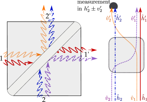
Figure 10: Polarizing beamsplitter transmits horizontally polarized photons and reflects vertically polarized ones, entangling the input state in the output modes. Subsequent polarization measurement in the diagonal basis of one of the output modes is a basis for type 1 fusion gate, which is used in generation of larger graph states from Bell pairs.

Optical realizations [41], while using different mechanisms for entangling, lead to a similar result. If a type 1 entangling gate is used, imperfect mode matching leads affected qubits to be effectively depolarized in the $Z$ basis. This has the exact same result on the output state as local (single-qubit) phase noise, despite different physical origins. A different scheme for generating large cluster states is employed in linear optics experiments. In such systems, the qubits are encoded as photons in different light modes. Two modes are associated with each qubit, and a single photon being in one of them corresponds to the standard computational basis states. Usually, these are polarization (horizontal/vertical) modes with overlapping spatial profiles. Thus, let us denote the creation operators of those modes by ${\hat{h}^{\dagger}}_{i}$ and ${\hat{v}^{\dagger}}_{i}$.

In this context, a Bell pair encoded as the nontrivial two-vertex graph state can be written as

$$\ket{{\bullet\!\!-\!\!\bullet}}=\frac{1}{2}(1,1,1,-1)^{T}=\frac{{\hat{h}^{\dagger}}_{1}{\hat{h}^{\dagger}}_{2}+{\hat{v}^{\dagger}}_{1}{\hat{h}^{\dagger}}_{2}+{\hat{h}^{\dagger}}_{1}{\hat{v}^{\dagger}}_{2}-{\hat{v}^{\dagger}}_{1}{\hat{v}^{\dagger}}_{2}}{2}\ket{\emptyset},$$ (39)

where $\ket{\emptyset}$ denotes the vacuum state of the optical field. For creation of a larger graph states, $N$ such Bell pairs generated through spontaneous parametric downconversion, with the initial state of

$$\ket{{\bullet\!\!-\!\!\bullet}}^{\otimes N}=\prod_{i=1}^{N}\frac{{\hat{h}^{\dagger}}_{2i-1}{\hat{h}^{\dagger}}_{2i}+{\hat{v}^{\dagger}}_{2i-1}{\hat{h}^{\dagger}}_{2i}+{\hat{h}^{\dagger}}_{2i-1}{\hat{v}^{\dagger}}_{2i}-{\hat{v}^{\dagger}}_{2i-1}{\hat{v}^{\dagger}}_{2i}}{2}\ket{\emptyset}.$$ (40)

The Bell pairs are subsequently fused to create a larger graph state. Every fusion takes two spatial modes (indexed by numbers in the subscription) and mixes them through a polarizing beamsplitter – see Figure 10 for the details. Then, one of the output modes is measured in the diagonal $h\pm v$ polarization basis. To see the effect of such operation, consider arbitrary input graph state (not necessarily a tensor product of Bell pairs) for graph $G=(V,E)$ such that the vertices 1 and 2 are not connected:

$$\ket{G} =\prod_{\{1,j\}\in E}\operatorname{CZ}_{1,i}\prod_{\{2,j\}\in E}\operatorname{CZ}_{2,j}\ket{+}\otimes\ket{+}\otimes\ket{G^{\prime}}$$ (41)

$$=\frac{{\hat{h}^{\dagger}}_{1}{\hat{h}^{\dagger}}_{2}f_{++}+{\hat{v}^{\dagger}}_{1}{\hat{h}^{\dagger}}_{2}f_{-+}+{\hat{h}^{\dagger}}_{1}{\hat{v}^{\dagger}}_{2}f_{+-}+{\hat{v}^{\dagger}}_{1}{\hat{v}^{\dagger}}_{2}f_{--}}{2}\ket{\emptyset},$$

where the symbols $f$ denote expressions involving creation operators to arrive at the state $\ket{\psi}$. The $f_{++}$ prepares the graph state $\ket{G^{\prime}}$, while $f_{-+}$ creates the state $\prod_{(1,i)\in G}z_{i}\ket{G^{\prime}}$: it is the postselected graph state upon measuring negative sign of the first qubit in the $Z$ basis. The other two operators work similarly; however, $f_{--}$ flips the phase of $\ket{G^{\prime}}$ only in the qubits that are connected to only $1$ or $2$.

Polarizing beamsplitter exchanges the vertical polarization, keeping the horizontal ones intact ($U{\hat{h}^{\dagger}}_{1,2}={\hat{h}^{\dagger}}_{1,2}U$, $U{\hat{v}^{\dagger}}_{1,2}={\hat{v}^{\dagger}}_{2,1}U$):

$$U\ket{G} =\frac{{\hat{h}^{\dagger}}_{1}{\hat{h}^{\dagger}}_{2}f_{++}+{\hat{v}^{\dagger}}_{2}{\hat{h}^{\dagger}}_{2}f_{-+}+{\hat{h}^{\dagger}}_{1}{\hat{v}^{\dagger}}_{1}f_{+-}+{\hat{v}^{\dagger}}_{1}{\hat{v}^{\dagger}}_{2}f_{--}}{2}\ket{\emptyset}.$$ (42)

The spatial mode 2 is subsequently measured in the basis of $({\hat{h}^{\dagger}}_{2}\pm{\hat{v}^{\dagger}}_{2})\ket{\emptyset}$, corresponding to the $\ket{\pm}$ of the logical qubit. If only a single $h+v$ photon is detected, the postselected output state reads

$$\frac{{\hat{h}^{\dagger}}_{1}f_{++}+{\hat{v}^{\dagger}}_{1}f_{--}}{\sqrt{2}}\ket{\emptyset}.$$ (43)

This is exactly the state corresponding to a graph $G^{\prime\prime}=(V^{\prime\prime},E^{\prime\prime})$ for which vertices 1 and 2 were merged with duplicate edges removed: $E^{\prime\prime}=E^{\prime}\cup\{\{1,i\}:\{1,i\}\in E\veebar\{2,i\}\in E\}$.

This is the case only if the photons in modes 1 and 2 are indistinguishable after mixing through the polarizing beamsplitter – the procedure relies on the Hong-Ou-Mandel effect. Shall this assumption not be met, the interference required for the fusion to work does not take place, and effectively the two photons originating in mode 1 and 2 are measured independently. If only one photon was observed in the new mode 2, half of the times it arrived from the mode (1,v), while the photon from mode 2 is now localized in the new mode (1,v) and the final state is ${\hat{v}^{\dagger}}_{1}f_{--}\ket{\emptyset}$. The opposite process means that the resulting state ${\hat{h}^{\dagger}}_{1}f_{++}\ket{\emptyset}$.

This effectively creates an ensemble which allows for the following interpretation: the fusion took place as if the photons were indistinguishable, but it was immediately measured in the $Z_{1}$ basis and the result of measurement is not known. This is equivalent to a simple probabilistic $Z_{1}$ flip:

$$\overbrace{\Pi_{Z_{1}+}}^{\frac{1}{2}(1+Z_{1})}\rho\Pi_{Z+}+\overbrace{\Pi_{Z_{1}-}}^{\frac{1}{2}({1-Z_{1}})}\rho\Pi_{Z_{1}-}=\frac{\rho+Z_{1}\rho Z_{1}}{2}.$$ (44)

The $Z$-flip ensemble is equivalent to $Z$-measurement one and is easier to work with. It is easier to observe that the noise does not propagate if the affected qubit is then fused with others, since there is always just a (potentially $Z$-flipped) graph state at the input – unless it also fails because the noise is correlated.

References

- [1] R. Raussendorf and H. J. Briegel. “A one-way quantum computer”. Phys. Rev. Lett. 86, 5188 (2001).
- [2] M. A. Nielsen. “Cluster-state quantum computation”. Rep. Math. Phys. 57, 147 (2006).
- [3] R. Raussendorf, D. E. Browne, and H. J. Briegel. “Measurement-based quantum computation on cluster states”. Phys. Rev. A 68, 022312 (2003).
- [4] M. Rossi, M. Huber, D. Bruß, and C. Macchiavello. “Quantum hypergraph states”. New J. Phys. 15, 113022 (2013).
- [5] M. Hein, W. Dür, J. Eisert, et al. “Entanglement in graph states and its applications”. arXiv:quant-ph/0602096, Proceedings of the International School of Physics “Enrico Fermi” 162, 115 (2006).
- [6] C. Kruszynska and B. Kraus. “Local entanglability and multipartite entanglement”. Phys. Rev. A 79, 052304 (2009).
- [7] R. Qu, J. Wang, Z.-S. Li, and Y.-R. Bao. “Encoding hypergraphs into quantum states”. Phys. Rev. A 87, 022311 (2013).
- [8] M. Gachechiladze, O. Gühne, and A. Miyake. “Changing the circuit-depth complexity of measurement-based quantum computation with hypergraph states”. Phys. Rev. A 99, 052304 (2019).
- [9] L. Vandré and O. Gühne. “Entanglement purification of hypergraph states”. Phys. Rev. A 108, 062417 (2023).
- [10] C. H. Bennett, G. Brassard, C. Crépeau, et al. “Teleporting an unknown quantum state via dual classical and Einstein-Podolsky-Rosen channels”. Phys. Rev. Lett. 70, 1895 (1993).
- [11] D. Bouwmeester, J.-W. Pan, K. Mattle, et al. “Experimental quantum teleportation”. Nature 390, 575 (1997).
- [12] M. F. Mor-Ruiz and W. Dür. “Influence of noise in entanglement-based quantum networks” (2023). arXiv:2305.03759.
- [13] R. Frantzeskakis, C. Liu, Z. Raissi, et al. “Extracting perfect GHZ states from imperfect weighted graph states via entanglement concentration”. Phys. Rev. Res. 5, 023124 (2023).
- [14] S. Morley-Short, M. Gimeno-Segovia, T. Rudolph, and H. Cable. “Loss-tolerant teleportation on large stabilizer states”. Quantum Sci. Technol. 4, 025014 (2019).
- [15] T. Wagner, H. Kampermann, D. Bruß, and M. Kliesch. “Learning logical Pauli noise in quantum error correction”. Phys. Rev. Lett. 130, 200601 (2023).
- [16] D. Miller, D. Loss, I. Tavernelli, et al. “Shor–Laflamme distributions of graph states and noise robustness of entanglement”. J. Phys. A 56, 335303 (2023).
- [17] J. de Jong, F. Hahn, N. Tcholtchev, et al. “Extracting GHZ states from linear cluster states” (2023). arXiv:2211.16758.
- [18] M. F. Mor-Ruiz and W. Dür. “Noisy stabilizer formalism”. Phys. Rev. A 107, 032424 (2023).
- [19] V. Mannalath and A. Pathak. “Multiparty entanglement routing in quantum networks”. Phys. Rev. A 108, 062614 (2023).
- [20] F. Hahn, A. Pappa, and J. Eisert. “Quantum network routing and local complementation”. npj Quantum Information 5, 76 (2019).
- [21] J.-Y. Wu, H. Kampermann, and D. Bruß. “Determining X-chains in graph states”. J. Phys. A 49, 055302 (2015).
- [22] L. Hartmann, J. Calsamiglia, W. Dür, and H. J. Briegel. “Weighted graph states and applications to spin chains, lattices and gases”. J. Phys. B 40, S1 (2007).
- [23] D. M. Greenberger, M. A. Horne, and A. Zeilinger. “Going beyond Bell’s theorem”. In Bell’s theorem, Quantum Theory and Conceptions of the Universe. Page 69. Springer (1989).
- [24] S. Cao, B. Wu, F. Chen, et al. “Generation of genuine entanglement up to 51 superconducting qubits”. Nature 619, 738 (2023).
- [25] P. Thomas, L. Ruscio, O. Morin, and G. Rempe. “Efficient generation of entangled multiphoton graph states from a single atom”. Nature 608, 677 (2022).
- [26] M. Van den Nest, J. Dehaene, and B. De Moor. “Graphical description of the action of local Clifford transformations on graph states”. Phys. Rev. A 69, 022316 (2004).
- [27] V. Mannalath and A. Pathak. “Entanglement routing and bottlenecks in grid networks” (2023). arXiv:2211.12535.
- [28] J. Stehlik, D. M. Zajac, D. L. Underwood, et al. “Tunable coupling architecture for fixed-frequency transmon superconducting qubits”. Phys. Rev. Lett. 127, 080505 (2021).
- [29] J. Long, T. Zhao, M. Bal, et al. “A universal quantum gate set for transmon qubits with strong ZZ interactions” (2021). arXiv:2103.12305.
- [30] H. Wunderlich, C. Wunderlich, K. Singer, and F. Schmidt-Kaler. “Two-dimensional cluster-state preparation with linear ion traps”. Phys. Rev. A 79, 052324 (2009).
- [31] C. Piltz, T. Sriarunothai, A.F. Varón, and C. Wunderlich. “A trapped-ion-based quantum byte with next-neighbour cross-talk”. Nat. Commun. 5, 052324 (2014).
- [32] J.-Y. Wu, M. Rossi, H. Kampermann, et al. “Randomized graph states and their entanglement properties”. Phys. Rev. A 89, 052335 (2014).
- [33] P. Erdős and A. Rényi. “On random graphs. I.”. Publ. Math. 6, 290 (2022).
- [34] D. E. Browne and T. Rudolph. “Resource-efficient linear optical quantum computation”. Phys. Rev. Lett. 95, 010501 (2005).
- [35] P. P. Rohde and T. C. Ralph. “Error models for mode mismatch in linear optics quantum computing”. Phys. Rev. A 73, 062312 (2006).
- [36] S. Rahimi-Keshari, T. C. Ralph, and C. M. Caves. “Sufficient conditions for efficient classical simulation of quantum optics”. Phys. Rev. X 6, 021039 (2016).
- [37] J. Anders, E. Andersson, D. E Browne, et al. “Ancilla-driven quantum computation with twisted graph states”. Theor Comput Sci 430, 51 (2012).
- [38] T. Rudolph. “Why I am optimistic about the silicon-photonic route to quantum computing”. APL photonics 2, 030901 (2017).
- [39] N. Shettell and D. Markham. “Graph states as a resource for quantum metrology”. Phys. Rev. Lett. 124, 110502 (2020).
- [40] G. Li, Y. Ding, and Y. Xie. “Tackling the qubit mapping problem for NISQ-era quantum devices”. In Proceedings of the Twenty-Fourth International Conference on Architectural Support for Programming Languages and Operating Systems. ASPLOS ’19. ACM (2019).
- [41] C.-Y. Lu, X.-Q. Zhou, O. Gühne, et al. “Experimental entanglement of six photons in graph states”. Nat. Phys. 3, 91 (2007).