pop-cosmos: A comprehensive picture of the galaxy population from COSMOS data

Abstract

We present pop-cosmos: a comprehensive model characterizing the galaxy population, calibrated to $140,938$ galaxies from the Cosmic Evolution Survey (COSMOS) with photometry in $26$ bands from the ultra-violet to the infra-red. We construct a detailed forward model for the COSMOS data, comprising: a population model describing the joint distribution of galaxy characteristics and its evolution (parameterized by a flexible score-based diffusion model); a state-of-the-art stellar population synthesis (SPS) model connecting galaxies’ instrinsic properties to their photometry; and a data-model for the observation, calibration and selection processes. By minimizing the optimal transport distance between synthetic and real data we are able to jointly fit the population- and data-models, leading to robustly calibrated population-level inferences that account for parameter degeneracies, photometric noise and calibration, and selection effects. We present a number of key predictions from our model of interest for cosmology and galaxy evolution, including the mass function and redshift distribution; the mass-metallicity-redshift and fundamental metallicity relations; the star-forming sequence; the relation between dust attenuation and stellar mass, star formation rate and attenuation-law index; and the relation between gas-ionization and star formation. Our model encodes a comprehensive picture of galaxy evolution that faithfully predicts galaxy colors across a broad redshift ($z<4$) and wavelength range.

1 Introduction

As galaxies evolve, their macroscopic (astro)physical characteristics – stellar mass, metallicity, dust, gas and active galactic nuclei (AGN) content – will evolve accordingly. While the detailed physics of galaxy-evolution and merger histories is not directly observable for individual galaxies, these processes determine the joint distribution of physical characteristics in the galaxy population, and how that distribution evolves over cosmic time. Constraining the joint distribution of galaxy properties in the Universe is therefore one of the main ways we can learn about galaxy evolution (see e.g. Madau & Dickinson, 2014 for a broad review).

As well as enabling galaxy evolution science, detailed characterization of the galaxy demographics over cosmic history is critical for cosmological probes that rely on observations of galaxies. Large-scale galaxy imaging surveys, which probe cosmological structure formation via galaxy clustering and weak gravitational lensing, require accurate determination of galaxy redshifts from their broad-band photometry. The physical characteristics of galaxies uniquely determine their spectral energy distributions (SEDs; e.g. Conroy, 2013), providing the link between prediction and observation in inferring redshifts from photometric data. The joint distribution of galaxy properties implicitly provides the prior over galaxy SEDs, which is critical for accurate photometric redshift estimation (especially from broad-band data: Arnouts et al., 1999; Benitez, 2000; Ilbert et al., 2006; Brammer et al., 2008; Tanaka, 2015). In Alsing et al. (2023) we recently showed that the redshift distributions of ensembles of galaxies in photometric surveys can be accurately derived via forward modeling, i.e., explicit modeling of the galaxy population, observational processes, and selection effects, provided those elements can be modeled with sufficiently high fidelity. Accurate estimation of redshift distributions is essential for obtaining robust and accurate cosmological constraints, and currently represents one of the main systematic challenges for both current (Stage III) and imminent (Stage IV) surveys, such as the Dark Energy Survey (DES; Flaugher, 2005), the Kilo Degree Survey (KiDS; De Jong et al., 2015) and Hyper Suprime-Cam (HSC; Aihara et al., 2018), the Vera C. Rubin Observatory’s Legacy Survey of Space and Time (LSST; Abell et al., 2009), and Euclid (Laureijs et al., 2011).

In addition, in order to leverage the cosmological information from small-scale galaxy-clustering, we require an understanding of how galaxies with different properties trace the underlying dark matter field (ie., galaxy bias, Sheth & Tormen, 1999; Tinker et al., 2010). Detailed characterization of the galaxy population is hence a key component in the exploration and exploitation of the galaxy-halo connection (see e.g. Wechsler & Tinker, 2018 for a recent review).

Furthermore, for transient cosmology (e.g. with type Ia supernovae; SNe Ia), understanding the properties of supernova host galaxies and how they correlate with intrinsic supernovae characteristics and observables is essential for drawing robust cosmological inferences. Host galaxy information has been shown to have relevance to supernova and transient classification (see e.g. Foley & Mandel, 2013; Gagliano et al., 2021, 2023). For SNe Ia, there are models connecting galaxy evolution to possible progenitor channels (e.g. Scannapieco & Bildsten, 2005; Mannucci et al., 2005, 2006; Childress et al., 2014). There are also poorly-understood correlations between SN Ia magnitudes and the mass or star formation rate of their hosts (e.g. Kelly et al., 2010; Sullivan et al., 2010). There is considerable current debate in the literature regarding the root causes and nature of these correlations (see, e.g., Brout & Scolnic, 2021; Thorp et al., 2021; Nicolas et al., 2021; Thorp & Mandel, 2022; Briday et al., 2022; Meldorf et al., 2023; Duarte et al., 2023; Grayling et al., 2024). Resolving this question will be essential for next generation projects, and already presents a challenge to current experiments (e.g. Vincenzi et al., 2024)

In spite of its critical role in galaxy evolution, cosmology, and other fields, studies of the joint distribution of galaxy properties have largely focused on measuring specific scaling relations between two or three properties at a time, such as the (redshift evolving) mass function (Marchesini et al., 2009; Ilbert et al., 2013; Muzzin et al., 2013; Moustakas et al., 2013; Tomczak et al., 2014; Grazian et al., 2015; Song et al., 2016; Davidzon et al., 2017; Wright et al., 2018; Leja et al., 2020), the mass-metallicity and fundamental metallicity relations (star-formation rate vs. gas metallicity vs. mass; Tremonti et al., 2004; Maiolino et al., 2008; Mannucci et al., 2009; Lara-López et al., 2010; Yates et al., 2012; Lara-López et al., 2013; Andrews & Martini, 2013; Nakajima & Ouchi, 2014; Yabe et al., 2015; Salim et al., 2014, 2015; Kashino et al., 2016; Cresci et al., 2019; Cullen et al., 2021; Curti et al., 2020; Bellstedt et al., 2021; Sanders et al., 2021; Thorne et al., 2022), the connection between dust and gas properties and star-formation histories (Burgarella et al., 2005; Kriek & Conroy, 2013; Arnouts et al., 2013; Reddy et al., 2015; Salmon et al., 2016; Salim et al., 2016; Leja et al., 2017; Kaasinen et al., 2018; Tress et al., 2018; Salim & Narayanan, 2020; Nagaraj et al., 2022), and the star-forming sequence (star-formation rate vs. mass vs. redshift; Daddi et al., 2007; Noeske et al., 2007; Karim et al., 2011; Rodighiero et al., 2011; Whitaker et al., 2012, 2014; Speagle et al., 2014; Renzini & Peng, 2015; Schreiber et al., 2015; Tomczak et al., 2016; Leslie et al., 2020; Leja et al., 2022). In the case of spectroscopic studies, these relationships have typically been measured from carefully targeted subsets of galaxies, limiting their utility in describing the galaxy population at large. For studies based on larger photometric datasets, significant parameter degeneracies and uncertainties demand a principled (Bayesian hierarchical) approach to population-level inference, which can properly account for those effects; this has so far not been achieved.

In order to be useful in a cosmological inference context – and to provide a more complete picture of the demographics of the galaxy population in general – it is desirable to obtain comprehensive constraints on the joint density $P(\bm{\varphi})$ of galaxy characteristics $\bm{\varphi}$, from a large and deep sample of galaxies, with as simple selection criteria as possible, and with any selection effects properly accounted and corrected for.

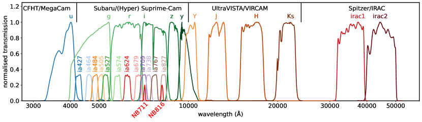
Figure 1: The subset of 26 COSMOS bands use in this work. Broadband transmission curves are rescaled to have peak transmission of 1.0, intermediate bands (“ia…”) are scaled to peak at $1/3$, and narrow bands (“NB…”) to peak at 0.2.

In this work we fit a flexible, non-parametric model for the joint density of galaxy characteristics to a large, deep ($r<25$), flux-limited sample of galaxies from the Cosmic Evolution Survey (COSMOS; Scoville et al., 2007; Weaver et al., 2022), assuming a state-of-the-art stellar population synthesis (SPS) model connecting galaxy properties with their SEDs. We construct a detailed forward model for the COSMOS data, accounting for photometric noise and calibration, selection effects, and modeling biases at the level of the SPS predictions. We then use simulation-based inference (SBI) to jointly fit the population model along with photometric noise and calibration parameters (and modeling errors), while properly accounting and correcting for selection effects. The result is a robustly calibrated galaxy population model that characterizes the complex web of dependencies between galaxy characteristics, and how they evolve over cosmic time.

Our calibrated population model, which we denote pop-cosmos, is useful for both cosmological applications and galaxy evolution studies, and is the first joint inference of the full set of dependencies between galaxy characteristics (rather than individual scaling-relations), while properly accounting for degeneracies between parameters, calibration and selection effects in a principled fashion.

This represents a milestone in our ongoing effort to achieve accurate galaxy-population modeling under SPS models. In Alsing et al. (2020) we developed neural emulation of SPS, achieving the ($10000\times$) speed-up required to deploy them at scale. In Alsing et al. (2023) we developed the forward modeling framework, demonstrating that existing state-of-the-art population modeling can already deliver (for example) redshift distributions accurate enough for Stage III surveys. In Leistedt et al. (2023) we developed the necessary photometric- and model-calibration elements, demonstrating state-of-the-art photo-$z$ performance. Now in the present work, we combine these advances with a flexible population-model parameterization and simulation-based inference to deliver comprehensive constraints on the galaxy population from a large, deep galaxy sample with broad wavelength coverage.

This paper is structured as follows. In §2 we describe the COSMOS galaxy sample. In §3 we describe the forward model, comprising the population model (§3.2), SPS model (§3.3), calibration and noise model (§3.4), and selection. The optimal-transport based simulation-based inference technique is described in §4. Results are presented in §5, with discussion and conclusions in §6 and §7.

2 Data

The Cosmic Evolution Survey (COSMOS), comprises deep imaging and photometry (in 44 bands) of $1.7$ million objects across $2\,\mathrm{deg}^{2}$ in the COSMOS field (Weaver et al., 2022). We use profile-fitting based photometry from the Farmer (COSMOS2020) catalog (Weaver et al., 2022, 2023a) in 26 of the available bands, chosen to ensure well-calibrated photometry and relatively homogeneous depth across wavelengths (following Brammer et al., 2008; Leistedt et al., 2023; see our Figure 1). This selection excludes the Subaru Suprime-Cam broad bands (which are shallower than other filters at similar wavelengths), and the GALEX bands (which are shallow and also have broad PSFs; Weaver et al., 2022).

We apply the conservative combined mask, which retains the deepest regions with the greatest number of available bands while removing areas corrupted by bright stars and other artifacts (Weaver et al., 2022). The catalog is prepared using the code released with the COSMOS2020 data, which applies the relevant flux corrections (including Galactic extinction) and unit conversions. We use the same star–galaxy separation criterion as Weaver et al. (2022), which is based on the $\chi^{2}$ estimated for star and galaxy templates in LePhare (Arnouts et al., 1999; Ilbert et al., 2006) as well as morphology information from the COSMOS HST/ACS mosaics.

To construct a clean and complete analysis sample, we impose a hard magnitude cut in the $r$-band of $r<25$, two magnitudes shallower than the 3$\sigma$ magnitude limit. This results in a flux-limited sample of $140,938$ galaxies, without significant additional selection effects.

Table 1: Summary of key notation and SPS model parameters.

Symbol	Description	Details
	Population-level hyperparameters
$\bm{\psi}$	Population model hyperparameters (weights and biases of the diffusion model)	§3.2
$\bm{\mu}(\mathbf{f})$	Flux-dependent mean of uncertainty model	§3.4
$\bm{\Sigma}(\mathbf{f})$	Flux-dependent std. dev. of uncertainty model	§3.4
$\bm{\chi}$	Uncertainty model hyperparameters (weights and biases of the MDN)	§3.4
$\bm{\alpha}_{\mathrm{ZP}}$	Zero-point corrections ($\times 26$)	§3.1
$\bm{\beta}_{\mathrm{EM}}$	Emission line (fractional) corrections relative to CLOUDY ($\times 44$)	Tab. 2, §3.1
$\bm{\gamma}_{\mathrm{EM}}$	Fractional variance in emission line contributions ($\times 44$)	Tab. 2, §3.1
$\bm{\eta}$	All “nuicance” parameters $\{\bm{\chi},\bm{\alpha}_{\mathrm{ZP}},\bm{\beta}_{\mathrm{EM}},\bm{\gamma}_{\mathrm{EM}}\}$	§4
	Galaxy-level quantities
$\bm{\varphi}$	SPS model parameters	Tab. 1, §3.3
$f_{b}^{\mathrm{SPS}}(\bm{\varphi},z)$	SPS model flux in band $b$	Eq. (1), §3.1
$\mathbf{f}_{b}^{\mathrm{EM}}(\bm{\varphi},z)$	Vector of emission-line contributions to the flux in band $b$	§3.1
$f_{b}(\bm{\varphi},z)$	Total model flux in band $b$	Eq. (2), §3.1
$\mathbf{f}$	True model flux in all bands $\{f_{1:26}(\bm{\varphi},z)\}$	§3.1
$\bm{\sigma}_{\mathrm{P}}$	Photometric uncertainty	Eq. (10), §3.1, §3.4
$\bm{\sigma}_{\mathrm{EM}}$	Uncertainty due to un-modeled emission line variations	Eq. (3), §3.1
$\bm{\sigma}$	Total noise standard deviation ($\bm{\sigma}^{2}=\bm{\sigma}^{2}_{\mathrm{P}}+\bm{\sigma}^{2}_{\mathrm{EM}}$)	§3.1
$\mathbf{d}$	Vector of noisy, calibrated model fluxes	Eq. (4), §3.1
$\hat{\mathbf{d}}$	Vector of observed fluxes	§4
$\bm{u},\bm{s}\sim\mathcal{N}(0,1)$	Base normal random variates for population and uncertainty models	§3.4, §4
$\bm{n}\sim\mathcal{T}_{2}$	Base Student’s-$t$ variates for the noise model	§3.1, §4
$\mathbf{D}$	Full sample of mock photometry (ie., a mock catalog realization), $\mathbf{D}=\{\mathbf{d}\}_{1:N}$	§4
$\hat{\mathbf{D}}$	Observed catalog of COSMOS photometry, $\hat{\mathbf{D}}=\{\hat{\mathbf{d}}\}_{1:N}$	§4
	Distributions and functions
$P(\bm{\varphi},z|\bm{\psi})$	Population model (score-based diffusion model)	§3.2
$P(\bm{\sigma}_{\mathrm{P}}|\mathbf{f};\bm{\chi})$	Uncertainty model (mixture density network)	§3.4
$P(\mathbf{n})$	Whitened noise distribution (independent Student’s-$t$, 2 d.o.f.)	Eq. (4), §4
$\mathcal{W}_{2}(\mathbf{D},\hat{\mathbf{D}})$	Optimal transport distance between $\mathbf{D}$ and $\hat{\mathbf{D}}$	§4
	SPS model parameters	Prior Limits
$z$	Redshift	$[0.0,4.5]$
$\mathrm{log}_{10}(M/M_{\odot})$	Stellar mass	$[7.0,13.0]$
$\Delta\mathrm{log}_{10}(\text{SFR})$	Logarithm of ratios of SFR between redshift bins ($\times 6$)	$[-5.0,5.0]$
$\tau_{1}$	Optical depth of dust in birth cloud	$[0.0,2.0]$
$\tau_{2}$	Optical depth of diffuse dust	$[0.0,4.0]$
$n$	Index of dust attenuation law	$[-1.0,0.4]$
$\mathrm{ln}(f_{\text{AGN}})$	Fractional contribution of AGN to luminosity	$[\mathrm{ln}(10^{-5}),\mathrm{ln}(3)]$
$\mathrm{ln}(\tau_{\text{AGN}})$	Optical depth of AGN dust torus	$[\mathrm{ln}(5),\mathrm{ln}(150)]$
$\mathrm{log}_{10}(Z_{\text{gas}}/Z_{\odot})$	Gas-phase metallicity	$[-2.0,0.5]$
$\mathrm{log}_{10}(U_{\text{gas}})$	Gas ionization	$[-4.0,-1.0]$
$\mathrm{log}_{10}(Z/Z_{\odot})$	Stellar metallicity	$[-1.98,0.19]$

3 Model

Our generative model for photometric galaxy survey data comprises a sequence of steps for simulating mock galaxy catalogs, which can then be compared against the observed data in a simulation-based inference setting for estimating the population-level parameters of interest (as described in §4). Notation is summarized in Table 1, the overall model structure and key components are outlined in §3.1, while the detailed assumptions about each model component are given in §3.2–3.4. The logical flow of our forward model is also summarized in Figure 2 (left panel).

3.1 Generative model structure

Our generative model proceeds in the following sequence of steps:

1. Draw galaxy parameters: SPS parameters $\bm{\varphi}$ and redshifts $z$ are drawn for each galaxy from the population-model $P(\bm{\varphi},z|\bm{\psi})$. Inference of the population model parameters $\bm{\psi}$ is the main target of our analysis. We parameterize $P(\bm{\varphi},z|\bm{\psi})$ as a score-based diffusion model (Song & Ermon, 2019; Song et al., 2020a, b; see §3.2 for details);

2. Compute photometry: Rest-frame spectral energy distributions (SEDs) $l(\lambda;\bm{\varphi})$ are calculated for each galaxy, given its SPS parameters $\bm{\varphi}$ and the assumed SPS model. The photometry $f_{b}$ in each band $b$, for each galaxy, is then obtained by:

   $$f {}^{\mathrm{SPS}}_{b}(\bm{\varphi},z)=$$

   $$\frac{(1+z)^{-1}}{4\pi d_{L}^{2}(z)}\int_{0}^{\infty}l(\lambda/(1+z);\bm{\varphi})e^{-\tau(z,\lambda)}W_{b}(\lambda)d\lambda,$$ (1)

   where $d_{L}(z)$ the luminosity distance for redshift $z$, $\tau(z,\lambda)$ is the optical depth of the inter-galactic medium, and $W_{b}(\lambda)$ are the band-passes for each band $b$. We assume a state-of-the-art $16$-parameter SPS model, detailed in §3.3;

3. Calibrate photometry: Measured photometry is subject to calibration biases. We apply zero-point corrections $\alpha_{\mathrm{ZP}}$ per band. The SPS model, too, will be subject to small biases due to approximations and missing model components. For example, emission-line predictions are often only accurate at the $\mathcal{O}(10\%)$ level or less (Leistedt et al., 2023), with variation arising from both the SPS treatment used (e.g. Byler et al., 2017), and the scheme used to compute line intensities (quantum mechanical vs. semi-classical, etc.; see Guzmán et al., 2017; Ferland et al., 2017). In this step, we apply the zero-point $\alpha_{\mathrm{ZP}}$ and emission-line $\beta_{\mathrm{EM}}$ corrections to the SPS model photometry from step 2:

   $$f_{b}(\bm{\varphi},z)=\alpha_{\mathrm{ZP}}[f^{\mathrm{SPS}}_{b}(\bm{\varphi},z)+\bm{\beta}_{\mathrm{EM}}\cdot\mathbf{f}^{\mathrm{EM}}_{b}(\bm{\varphi},z)],$$ (2)

   where $\mathbf{f}^{\mathrm{EM}}_{b}(\bm{\varphi},z)$ is the vector of emission-line contributions to the photometry for band $b$. We include emission-line corrections to the $44$ strongest emission-lines, following Leistedt et al. (2023) (see our Table 2 for a list of included lines);

4. Draw uncertainties: We draw photometric uncertainties (noise variances) for each galaxy from an uncertainty model, $\bm{\sigma}_{\mathrm{P}}\leftarrow P(\bm{\sigma}_{\mathrm{P}}|\mathbf{f};\bm{\chi})$. The uncertainty model $P(\bm{\sigma}_{\mathrm{P}}|\mathbf{f};\bm{\chi})$, parameterized by $\bm{\chi}$, describes variation in photometric uncertainties from galaxy to galaxy due to heterogeneous observing conditions and strategy, varying difficulty in extracting photometry from galaxies with different morphologies and geometries, and the scaling of uncertainties with flux due to the Poisson photon count contribution to the measurement errors. Construction of the uncertainty model is detailed in §3.4.

   We model an additional source of photometric uncertainty arising from variability in the emission-line contributions to each galaxy (relative to CLOUDY predictions); these depend on the detailed micro-structure of the galaxy and are not captured in the SPS parameterization. To this end, we construct emission-line contributions to the photometric uncertainties in each band, parameterized as

   $$\sigma_{\mathrm{EM},b}=\bm{\gamma}_{\mathrm{EM}}(\bm{\beta}_{\mathrm{EM}}+1)\cdot\mathbf{f}^{\mathrm{EM}}_{b},$$ (3)

   where $\bm{\gamma}_{\mathrm{EM}}$ represent the (fractional) variance in the emission-line contributions for each of the $44$ lines included (Table 2). The total photometric uncertainty for each galaxy is then given by the quadrature sum of measurement and emission-line contributions $\bm{\sigma}^{2}=\bm{\sigma}_{\mathrm{P}}^{2}+\bm{\sigma}_{\mathrm{EM}}^{2}$;

5. Add noise: We add noise to the calibrated model photometry from step 3, given the photometric uncertainties from step 4, assuming independent Student’s-t errors on each band (with two degrees-of-freedom),

   $$\mathbf{d} =\mathbf{f}+\bm{\sigma}\odot\mathbf{n},$$

   $$P(n) =\frac{1}{2\sqrt{2}(1+n^{2}/2)^{3/2}},$$ (4)

   where $\mathbf{d}$ is the vector of noisy (calibrated) fluxes, $\odot$ denotes element-wise multiplication, and $\mathbf{f}$ denotes the vector of model fluxes (i.e. all the $f_{b}(\bm{\varphi},z)$ computed in step 3);

6. Apply selection: Galaxies are selected into the sample following the same photometric cuts that were applied to the data (§2).

This generative process represents a complete description of our model assumptions, or equivalently, our simulation pipeline for generating mock galaxy catalog data. Simulated catalogs generated in this way can be compared to the data in a simulation-based inference setting in order to estimate the population-level parameters (see §4).

In the following sections, we give more details of the population model (§3.2), SPS model (§3.3), and uncertainty model (§3.4) assumptions. The simulation-based fitting procedure is then described in §4.

Table 2: List of emission lines used, with our inferred fractional corrections ($\beta_{\mathrm{EM}}$) and variances ($\gamma_{\mathrm{EM}}$). Line wavelengths are from Byler et al. (2017), with the list of 44 selected lines being from Leistedt et al. (2023).

Line	$\lambda_{\mathrm{EM}}$ (Å)	$\beta_{\mathrm{EM}}$	$\gamma_{\mathrm{EM}}$
C ii] 2326	2326.11	$9.537\times 10^{-7}$	$1.425\times 10^{-13}$
[O iii] 2321	2321.66	$-9.060\times 10^{-6}$	$1.424\times 10^{-13}$
[O i] 6302	6302.05	$3.934\times 10^{-6}$	$1.464\times 10^{-13}$
[S ii] 4070	4069.75	$0.000\times 10^{0}$	$1.433\times 10^{-13}$
H i (Ly-$\alpha$)	1215.67	$1.073\times 10^{-6}$	$1.455\times 10^{-13}$
[Al ii] 2670	2669.95	$5.364\times 10^{-6}$	$1.425\times 10^{-13}$
[Ar iii] 7753	7753.19	$6.914\times 10^{-6}$	$1.427\times 10^{-13}$
H i (Pa-7)	9017.80	$3.934\times 10^{-6}$	$1.425\times 10^{-13}$
[Al ii] 2660	2661.15	$0.000\times 10^{0}$	$1.425\times 10^{-13}$
[S iii] 6314	6313.81	$-4.768\times 10^{-7}$	$1.426\times 10^{-13}$
H i (Pa-6)	9232.20	$-6.735\times 10^{-6}$	$1.426\times 10^{-13}$
[S iii] 3723	3722.75	$-1.311\times 10^{-6}$	$1.425\times 10^{-13}$
Mg ii 2800	2803.53	$-7.153\times 10^{-7}$	$1.434\times 10^{-13}$
H i (Pa-5)	9548.80	$-5.603\times 10^{-6}$	$1.427\times 10^{-13}$
He i 7065	7067.14	$-2.384\times 10^{-7}$	$1.427\times 10^{-13}$
[N ii] 6549	6549.86	$1.246\times 10^{-3}$	$2.163\times 10^{-13}$
[S ii] 6732	6732.67	$2.511\times 10^{-3}$	$3.600\times 10^{-13}$
C iii]	1908.73	$-4.411\times 10^{-6}$	$1.424\times 10^{-13}$
He i 6680	6679.99	$-6.497\times 10^{-6}$	$1.437\times 10^{-13}$
Mg ii 2800	2796.35	$-6.020\times 10^{-6}$	$1.460\times 10^{-13}$
[S ii] 6717	6718.29	$1.588\times 10^{-3}$	$1.028\times 10^{-13}$
[Ar iii] 7138	7137.77	$1.311\times 10^{-6}$	$1.490\times 10^{-13}$
[C iii]	1906.68	$6.199\times 10^{-6}$	$1.425\times 10^{-13}$
He i 4472	4472.73	$-1.788\times 10^{-6}$	$1.437\times 10^{-13}$
[O iii] 4364	4364.44	$-3.040\times 10^{-6}$	$1.425\times 10^{-13}$
[N ii] 6585	6585.27	$-6.017\times 10^{-1}$	$1.000\times 10^{-13}$
[S iii] 9071	9071.10	$-1.000\times 10^{0}$	$1.702\times 10^{-13}$
H-8 3798	3798.99	$8.345\times 10^{-6}$	$1.465\times 10^{-13}$
He i 3889	3889.75	$1.907\times 10^{-6}$	$1.500\times 10^{-13}$
H-7 3835	3836.49	$4.768\times 10^{-7}$	$1.485\times 10^{-13}$
[Ne iii] 3968	3968.59	$4.888\times 10^{-6}$	$1.448\times 10^{-13}$
He i 5877	5877.25	$3.242\times 10^{-1}$	$1.555\times 10^{-13}$
H-6 3889	3890.17	$-6.497\times 10^{-6}$	$1.536\times 10^{-13}$
[S iii] 9533	9533.20	$-1.000\times 10^{0}$	$2.017\times 10^{-13}$
H-5 3970	3971.20	$-1.409\times 10^{-1}$	$1.689\times 10^{-13}$
[O ii] 3726	3727.10	$2.513\times 10^{-3}$	$1.000\times 10^{-13}$
H-$\delta$ 4102	4102.89	$-5.149\times 10^{-1}$	$1.912\times 10^{-13}$
[O ii] 3729	3729.86	$2.619\times 10^{-1}$	$1.000\times 10^{-13}$
[Ne iii] 3870	3869.86	$-8.018\times 10^{-2}$	$1.889\times 10^{-13}$
H-$\gamma$ 4340	4341.69	$-3.312\times 10^{-1}$	$1.013\times 10^{-13}$
[O iii] 4960	4960.30	$-2.151\times 10^{-3}$	$1.000\times 10^{-13}$
H-$\beta$ 4861	4862.71	$-5.656\times 10^{-1}$	$1.000\times 10^{-13}$
H-$\alpha$ 6563	6564.60	$-3.409\times 10^{-1}$	$1.000\times 10^{-13}$
[O iii] 5007	5008.24	$1.136\times 10^{-1}$	$2.640\times 10^{-2}$

3.2 Population model

The population model $P(\bm{\varphi},z|\bm{\psi})$ is the main target of our analyses. We require a flexible parameterization for this high-dimensional density, which is capable of capturing the complex web of inter-dependencies between galaxies’ properties that arise from galaxy formation and evolution physics. Advances in generative machine-learning models, such as normalizing flows (Rippel & Adams, 2013; Germain et al., 2015; Dinh et al., 2016; Papamakarios et al., 2017; Grathwohl et al., 2018; Chen et al., 2018; Kingma & Dhariwal, 2018; Durkan et al., 2019; Papamakarios et al., 2021) and diffusion models (Sohl-Dickstein et al., 2015; Ho et al., 2020; Song & Ermon, 2019; Song et al., 2020b, a; Song & Ermon, 2020; Kingma et al., 2021; Luo, 2022) have provided a step change in our ability to parameterize and learn complex and high-dimensional probability distributions from data.

We parameterize $P(\bm{\varphi},z|\bm{\psi})$ using a score-based diffusion model (Song & Ermon, 2019; Song et al., 2020a, b), where the population-model parameters $\bm{\psi}$ are the weights and biases of the score-network (outlined below). Diffusion models have been shown to be effective flexible approximators for unknown probability distributions, are relatively inexpensive to train, and scale well to high-dimensional problems, making them ideally suited to this use-case (see Luo, 2022 for a review).

In diffusion models, as with normalizing flows, we aim to find an invertible transform that maps from some simple base density (eg., a unit normal) to our target $p(\bm{x})$, such that we can generate samples from the target by simply transforming draws from the base-density, ie.,

$$\bm{x}=\bm{f}(\bm{u}),\;\bm{u}\sim\mathcal{N}(0,1)$$

$$p(\bm{x})=\mathcal{N}(\bm{f}^{-1}(\bm{x})|0,1)|\bm{J}(\bm{x})|,$$ (5)

where $\bm{J}=\partial\bm{f}^{-1}(\bm{x})/\partial\bm{x}$ is the Jacobian, and the transform $\bm{f}$ must be invertible. In both normalizing flows and diffusion models, the goal is to parameterize the invertible transform $\bm{f}$ by a neural network.

In a score-based diffusion model, we begin by constructing a diffusion process $\{\bm{x}(t)\}_{t=1}^{t=T}$ (indexed by a continuous time-variable $t$) such that $\bm{x}(t=0)$ is distributed according to our target distribution, and $\bm{x}(t=T)$ has a normal distribution. This diffusion process can be described by a stochastic differential equation (SDE), which maps samples from our target distribution at $t=0$ to random noise at $t=T$:

$$d\bm{x}=\bm{f}(\bm{x},t)dt+g(t)d\bm{w},$$ (6)

where $\bm{w}$ is standard Brownian motion (Wiener process). In order to generate samples from our target then, we can take samples from the base normal distribution $\bm{x}(t=T)$ and reverse the process back to $t=0$. The reverse of a diffusion process defined by Equation (6) is simply another diffusion process, defined by the reverse-time SDE (Anderson, 1982; Song et al., 2020b):

$$d\bm{x}=\left[\bm{f}(\bm{x},t)+g(t)^{2}\nabla_{\bm{x}}p_{t}(\bm{x})\right]dt+g(t)d\bar{\bm{w}},$$ (7)

where $\bar{\bm{w}}$ is reverse-time Brownian motion, $p_{t}(\bm{x})$ are the marginal distributions of the diffusion process defined by Equation (6), and $dt$ is an infitesimal step backwards in time. Hence, once the score $\nabla_{\bm{x}}p_{t}(\bm{x})$ of the marginals of the forward diffusion process is known as a function of time, then the reverse-process in Equation (7) can be evaluated to transform samples from the base density $\bm{x}(t=T)\sim\mathcal{N}(0,1)$ to the target $\bm{x}(t=0)$. The transform from the base-density to the target is hence completely characterized by the score of the marginals: in a score-based diffusion model, the score $\bm{s}(\bm{x},t)=\nabla_{\bm{x}}p_{t}(\bm{x})$ is parameterized as a (dense) neural network, and fit by denoising score-matching (Hyvärinen, 2005; Song et al., 2020a, b, 2021), or otherwise.

So far, this reverse-time diffusion process provides a means to stochastically transform from the base density to the target, via Equation (7). However, in order to be able to evaluate the Jacobian and hence log probability, we require a deterministic (invertible) transform between the base and the target. Fortunately, for any reverse-time SDE of the form given in Equation (7), there exists a deterministic ordinary differential equation (ODE) that has the same marginal distributions as the SDE (Maoutsa et al., 2020; Song et al., 2020b):

$$d\mathbf{x}=\left[\bm{f}(\bm{x},t)-\frac{1}{2}g(t)^{2}\nabla_{\bm{x}}p_{t}(\bm{x})\right]dt.$$ (8)

Integrating this ODE from $t=T$ to $t=0$ hence provides a deterministic, invertible transform from the base density $\bm{x}(t=T)$ to the target $p(\bm{x})$, which is completely characterized by the score-function $\bm{s}(\bm{x},t)=\nabla_{\bm{x}}p_{t}(\bm{x})$, and whose Jacobian can be computed. Interpreting the diffusion model as an ODE transform in this way elicits an equivalence between continuous-time normalizing flows (Grathwohl et al., 2018; Chen et al., 2018) and score-based diffusion models (Song et al., 2020b).

We parameterize the score $\bm{s}(\bm{x},t)$ as a dense network with two layers of $128$ hidden units and tanh activation functions. We take the so-called variance-exploding SDE (Song et al., 2020b) to define the forward diffusion process,

$$d\mathbf{x}=g(t)d\bm{w},\;g(t)^{2}=\frac{d\sigma^{2}(t)}{dt},\;\sigma(t)=\sigma_{0}(\sigma_{T}/\sigma_{0})^{t/T},$$ (9)

where we choose $\sigma_{0}=0.01$, $\sigma_{T}=10$ and $T=1$, and implicitly in the variance-exploding SDE the drift-term $\bm{f}(\bm{x},t)$ is set to zero (c.f. Equation 6).

3.3 Stellar population synthesis (SPS) model

Stellar population synthesis provides the theoretical framework linking the stellar, gas and dust content of galaxies, and their SEDs (see Conroy, 2013 for a review). We assume a state-of-the-art $16$-parameter SPS model, based on the milestone Prospector-$\alpha$ model (Leja et al., 2017, 2018, 2019a, 2019b), but including the gas phase ionization parameter as an additional free parameter; we found that this additional parameter was required to give reasonable inferences about the gas-phase physics. For completeness, the physical assumptions and parameters are described below.

The star formation history (SFH) is modeled as piece-wise constant, with seven bins in time (see Leja et al., 2019a). The first two bins are fixed at $[0,30]$ Myr and $[30,100]$ Myr respectively, to capture recent star formation. The oldest bin is fixed at $[0.85,1]t_{\mathrm{age}}(z)$, where $t_{\mathrm{age}}(z)$ is the age of the universe at the lookback time of the galaxy. The remaining four bins are equally-spaced (logarithmically) in time between $100$ Myr and $0.85t_{\mathrm{age}}(z)$. The ratios of the log star formation rate (SFR) between adjacent SFH bins are then the free model parameters describing the SFH. This flexible six-parameter model is able to capture a rich diversity of SFH phenomenology, including both smooth and bursty star-formation histories.

Dust is modeled as separate diffuse and birth cloud dust screens, where the latter only impacts stars younger than $10$ Myr (Charlot & Fall, 2000). The optical depths $\tau_{1}$ (birth cloud) and $\tau_{2}$ (diffuse), as well as the power-law index of the Calzetti et al. (2000) attenuation curves, constitute the free parameters describing the dust model. Dust emission is powered by energy-balance.

The stellar metallicity for all stars in the galaxy is assumed to take a single value, ie., the model does not explicitly account for time-varying metallicity in the stellar population. This is generally a good approximation, although some studies suggest that metallicity evolution can improve SED modeling at the level of (typically) a few percent (Robotham et al., 2020; Bellstedt et al., 2020).

Gas is characterized by the gas-phase metallicity and ionization state. Nebular line and continuum emission is generated using CLOUDY (Ferland et al., 2013, 2017) model grids from Byler et al. (2017). We assume that the gas phase metallicity must be greater than or equal to the stellar metallicity (since the latter captures the light-weighted average over the stellar population, which includes older stars).

Active galactic nucleus (AGN) activity is modeled as described in Leja et al. (2018), where the fraction of the bolometric luminosity from the AGN $f_{\mathrm{AGN}}$ and optical depth of the AGN torus $\tau_{\mathrm{AGN}}$ are both included as free parameters.

Together with stellar mass and redshift, this amounts to a total of $16$ parameters characterizing each galaxy. The list of parameters and their prior limits are given in Table 1.

The SPS model is implemented in the public code Flexible Stellar Population Synthesis (FSPS; Conroy et al., 2009, 2010; Conroy & Gunn, 2010a, b), accessed through the python-fsps binding (Foreman-Mackey et al., 2014). We then use speculator (Alsing et al., 2020) to accelerate the SPS computation, achieving a factor of $10^{4}$ speed-up over FSPS per band, while maintaining sub-percent accuracy on the predicted fluxes.

3.4 Uncertainty model

The uncertainty model describes the distribution of photometric measurement uncertainties in the survey, conditional on the true source flux, $P(\bm{\sigma}_{\mathrm{P}}|\mathbf{f};\bm{\chi})$. Following Alsing et al. (2023), we model $P(\bm{\sigma}_{\mathrm{P}}|\mathbf{f};\bm{\chi})$ as a mixture density network (MDN; Bishop, 2006). Here we use an MDN with one Gaussian component, i.e., a neural network parameterizing the mean $\bm{\mu}(\mathbf{f})$ and standard deviation $\bm{\Sigma}(\mathbf{f})$ of the distribution of photometric uncertainties, conditioned on flux. From this, photometric uncertainties can be drawn for a simulated galaxy with flux $\mathbf{f}$ by drawing:

$$\bm{\sigma}_{\mathrm{P}}=\bm{\mu}(\mathbf{f})+\bm{\Sigma}(\mathbf{f})\odot\bm{s},\;\bm{s}\sim\mathcal{N}(0,1).$$ (10)

We parameterize the MDN with a single dense network with two hidden layers, with $128$ units each and tanh activation functions.

By keeping the uncertainty model parameters $\bm{\chi}$ free in the fitting process, we are able to fully self-calibrate the uncertainty model from the data, eliminating any reliance on the (approximate) estimated flux uncertainties in the Farmer catalog.

4 Inference

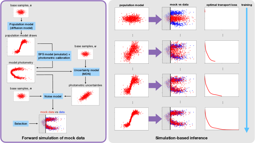
Figure 2: Left: Logical flow of our forward modeling (simulation) framework described in §3. Galaxy parameters are drawn from the population model (parameterized as a score-based diffusion model; § 3.2); calibrated model photometry are calculated assuming the SPS model (§ 3.3) and calibration models (Equation 2); photometric uncertainties are drawn from the uncertainty model (§ 3.4); photometric noise is drawn and added given the noise model (Equation 4); and finally selection is applied (§ 2). Note that the three stochastic steps (the population model, uncertainty model, and noise draws) are parameterized as bijective transforms from a base density (unit normal for the population- and uncertainty-model, and Student’s-t for the noise-model draws; see § 4). Right: Schematic illustration of our simulation-based inference framework, optimizing the optimal transport distance between simulated (red) and real (blue) data, by gradient descent. The forward modeling stages expanded in detail on the left are represented by the purple arrows in the right-hand block. Gradients of the simulator can be obtained via automatic differentiation, by keeping the input draws from the base density fixed in the forward simulations (see § 4).

Inferring the population-level parameters ${\bm{\psi},\bm{\eta}}$ from the hierarchical model defined in §3 is difficult for a number of reasons. Firstly, flexible (neural network) parameterizations of the population and photometric-uncertainty models mean that the number of hyper-parameters of interest is large. Secondly, there is a vast number of individual-galaxy level parameters $\{\bm{\varphi},z\}_{1:N}$ that would need to be inferred and then marginalized over in a typical Bayesian analysis (using e.g. Markov chain Monte Carlo methods). This provides a technical challenge due to the complexity and diversity of individual galaxy SPS-parameter likelihoods (degeneracies and multimodality are commonplace), and a computational bottleneck due to the large number of SPS model calls required. Thirdly, the selection effects introduce a high-dimensional integral into the likelihood, making it effectively intractable (see Alsing et al., 2023 for details).

Even though the likelihood is intractable, the model described in §3 defines a straightforward recipe for simulating mock catalogs, given some assumptions about the population-level parameters. This means that we may instead compare simulated catalogs to the data in a simulation-based inference setting, for example, by minimizing a suitable distance metric between model generated and real data.

Minimizing the divergence between the predictive (model) and true data distributions is well-motivated: maximum-likelihood estimation is asymptotically equivalent to minimizing the Kulback–Leibler (KL; Kullback & Leibler, 1951) divergence between model and data distributions. However, the KL divergence requires evaluating the predictive distribution for the data from our model, in this case the predicted distribution of galaxy photometry for galaxies in the survey (given hyper-parameters $\bm{\psi},\bm{\eta}$). As discussed above, this distribution is not tractable so we seek an alternative distance metric with properties suitable for robust and efficient parameter estimation.

We estimate the population-level parameters $\bm{\psi},\eta$ by minimizing the optimal transport (OT) distance between model generated data (catalog) $\mathbf{D}=\mathbf{d}_{1:N}$, and the COSMOS data $\hat{\mathbf{D}}=\hat{\mathbf{d}}_{1:N}$. The OT distance (also known as the Wasserstein distance or Kantorovich–Rubinstein metric, after Kantorovich & Rubinstein, 1958; Vaserstein, 1969) measures the divergence between two distributions from which we have samples, by computing the minimum distance required to transport one set of points onto the other, given some local metric to define distances in data space (for a review on OT and its implementation, see Peyré & Cuturi, 2019). Optimal transport has been widely used for parameter estimation in settings where the KL divergence is intractable (Peyré & Cuturi, 2019), providing efficient and consistent estimators, which are asymptotically equivalent to maximum-likelihood estimation in the large-dataset limit in most situations.

While exact calculation of the optimal transport distance is computationally complex ($\mathcal{O}{N^{3}\mathrm{ln}\,N}$; Pele & Werman, 2009) and difficult to scale, the Sinkhorn divergence (Cuturi, 2013) provides a fast ($\mathcal{O}{N^{2}\mathrm{ln}\,N}$; Altschuler et al., 2017; Dvurechensky et al., 2018) and accurate approximation. We use the Sinkhorn divergence implemented in pytorch (Paszke et al., 2019) in the geomloss library (Feydy et al., 2019) built on keops (Charlier et al., 2021), assuming a local Euclidean metric (2-norm) to define distances between data points.

The forward model described in §3 is stochastic: galaxy parameters are drawn from the population model distribution, calibrated model photometry is calculated and then uncertainties and noise are drawn and added, followed by application of selection cuts. In order to be able to use gradient-based optimization to minimize the OT distance between simulated and real data, we need to be able to take gradients through our simulator. To achieve this, we use a variant of the reparameterization trick (Kingma & Welling, 2013), where we re-write our forward model as a sequence of deterministic steps applied to some fixed draws from a base density (which are kept fixed for the purpose of estimating gradients). In this sense, our forward model can be written as the following sequence of steps:

1. Draw base random variates for the population-model, uncertainty-model, and noise-model:

   $$\bm{u}_{1:M}\sim\mathcal{N}(0,1),\;[\text{population-model base draws}]$$

   $$\bm{s}_{1:M}\sim\mathcal{N}(0,1),\;[\text{uncertainty-model base draws}]$$

   $$\bm{n}_{1:M}\sim\mathcal{T}_{2},\;[\text{noise-model base draws}]$$

   where $\mathcal{T}_{2}$ is the standard-$t$ distribution with two degrees-of-freedom (Equation 4), and $M$ is the number of mock galaxies to generate (which should be larger than the target (selected) catalog size $N$);

2. Pass base samples $\bm{u}_{1:M}$ to the population-model (score-based diffusion model) to generate draws of galaxy parameters $\bm{\varphi}_{1:M}$, by solving the ODE in Equation (8) (given the current values of the population-model parameters $\bm{\psi}$);

3. Compute calibrated photometry $\mathbf{f}_{1:M}$ for each galaxy assuming the SPS and calibration models (Equation 2, given the current values of the data-model parameters $\bm{\eta}$);

4. Pass base samples $\bm{s}_{1:M}$ and the model fluxes $\mathbf{f}_{1:M}$ through the uncertainty model (Equation 10) to generate photometric noise variances for each galaxy $\bm{\sigma}_{\mathrm{P},1:M}$ (given the current values of the uncertainty-model parameters $\bm{\chi}$);

5. Compute additional uncertainty contributions $\bm{\sigma}_{\mathrm{EM},1:M}$ due to emission-lines (Equation 3), and add in quadrature to get total uncertainties $\bm{\sigma}_{1:M}^{2}=\bm{\sigma}_{\mathrm{P},1:M}^{2}+\bm{\sigma}_{\mathrm{EM},1:M}^{2}$;

6. Pass base samples $\bm{n}_{1:M}$ and the model photometry to the noise model (Equation 4) to generate noisy mock photometry, $\mathbf{d}_{1:M}=\mathbf{f}_{1:M}+\bm{\sigma}_{1:M}\odot\bm{n}_{1:M}$;

7. Apply selection cuts (and trim the number of retained objects to $N$ if necessary) to give a mock catalog $\mathbf{D}(\bm{u},\bm{s},\bm{n}|\bm{\psi},\bm{\eta})=\{\mathbf{d}_{1:N},S_{1:N}=1\}$ of the desired size, $N$.

The objective function for minimization is then given by:

$$\mathcal{L}(\bm{\psi},\bm{\eta})=\mathcal{W}_{2}[\mathbf{D}(\bm{u},\bm{s},\bm{n}|\bm{\psi},\bm{\eta}),\hat{\mathbf{D}}],$$ (11)

where $\mathcal{W}_{2}$ denotes the OT distance (assuming a local Euclidean metric), $\mathbf{D}(\bm{u},\bm{s},\bm{n}|\bm{\psi},\bm{\eta})$ is the simulated catalog and $\hat{\mathbf{D}}$ the COSMOS catalog. By keeping the base random drawn from step 1 fixed, the simulated catalog (and hence OT distance) are deterministic functions of the parameters $\bm{\psi},\bm{\eta}$, so that we can take gradients and perform gradient-based optimization. This scheme is summarized in Figure 2.

4.1 Initialization and training

The calibration model parameters (characterizing the zero-points and emission-line corrections) are initialized following the Bayesian hierarchical calibration approach presented in Leistedt et al. (2023): cross-matching with data from zCosmos-bright (Lilly et al., 2007), DEIMOS (Hasinger et al., 2018)], and C3R2 (Masters et al., 2017, 2019; Stanford et al., 2021) yields 12,473 objects with spectroscopic redshifts available, in the range $0<z<2$. This lifts degeneracies between SPS parameters and makes the calibration model parameters very well constrained by the data. Simultaneous optimization of all parameters parameters converges easily, with the SPS parameter uncertainties having negligible effect on the result (see Leistedt et al., 2023 for more details).

To initialize the population model, we perform an initial maximum aposteriori (MAP) estimation of the SPS parameters for each galaxy in the COSMOS sample, and pre-train the diffusion model on that ensemble of MAP estimates via denoising score-matching. This provides a reasonable initialization for the population model to avoid a long burn-in phase based on the more expensive optimal transport objective.

The uncertainty model network is initialized as follows. The initial MAP estimates for the SPS parameters (and initialized calibration-model parameters) provide estimates of the true (denoised) photometry for each galaxy in the COSMOS sample. This provides a catalog of uncertainties and associated (denoised) photometry $\{\bm{\sigma}_{\mathrm{P}},\mathbf{f}\}$, on which we can train our conditional estimator for $P(\bm{\sigma}_{\mathrm{P}}|\mathbf{f};\bm{\chi})$ by minimizing the negative log-likelihood loss:

$$\mathcal{L}(\bm{\chi})=-\sum_{i=1}^{N_{\mathrm{train}}}\mathrm{ln}P(\bm{\sigma}_{\mathrm{P,}i}|\mathbf{f}_{i};\bm{\chi}).$$ (12)

This provides a reasonable initialization for the uncertainty model, after which $\bm{\chi}$ is kept free in the final fitting procedure.

OT optimization is then performed with Adam (Kingma & Ba, 2014) with a learning rate of $10^{-4}$, until the distance ceases to improve for twenty epochs. All of the population-level hyperparameters are kept free in the fitting process, with the exception of the zero points which we fix to their (Bayesian hierarchical) calibrated values: this is to avoid the exact degeneracy between the overall scale of the zero points and the normalization (i.e., stellar masses) of the observed photometry.

We compute the OT objective between both the synthetic and real magnitudes, and separately between the synthetic and real colors, and sum them. We find that this improves the ability of the fitted model to reproduce both the colors and magnitudes faithfully.

4.2 Discussion

The model fitting scheme described above has a number of advantages over existing methods.

Firstly, we target the hyper-parameters (describing population- and data-model) directly, completely bypassing the need to infer the properties of each individual galaxy in the sample (in contrast to eg., MCMC-based approaches). This provides a significant advantage in computational cost and scalability when population-level inference is the main goal.

Secondly, by jointly inferring the population- and data-model parameters together in a self-consistent fashion, we are able to use the data to “self-calibrate” any unknown nuisance parameters (e.g., calibration and noise-model parameters, etc). This will result in more robust inferences compared to the traditional approach of estimating and fixing nuisance parameter values prior to the main analysis.

Since our forward model explicitly accounts for selection effects, the resulting inferred population-model will have selection properly corrected for (effectively “deconvolved”). The resulting population model can then be straightforwardly utilized for prediction (and like-for-like comparison) for different surveys, simply by applying the noise characteristics and selection effects appropriate for that survey in a forward modeling context. This point is critical for application to cosmological inference from broad-band galaxy surveys, where we require a well-calibrated population model that is able to make faithful predictions for those deep, broad-band data. Note that while our method properly corrects for selection effects, it is not designed to extrapolate more than a few noise standard deviations below the flux-limit (where there is no data to constrain the population model). Therefore, application of the calibrated population model should be limited to surveys with similar or shallower depths.

Our forward modeling-based approach is also well suited to principled validation on the basis of predictive performance. This is in contrast to typical galaxy evolution and cosmology analyses, where population-level inferences are drawn, but little assessment of prediction quality (in data-space) is done. In a companion paper (Thorp et al., in prep.), we present a model validation approach for the simulation-based inference setting, based on quantile–quantile (QQ) and probability–probability (PP) plots (Wilk & Gnanadesikan, 1968; see Eadie et al., 2023 for an astronomy example). A further complication is the question of comparing models. Again, the most popular approaches in astrophysics and cosmology are typically applied at the level of the parameter posterior (i.e. via the Bayesian evidence; although use of posterior predictive scores is growing, see e.g. Feeney et al., 2019; Abbott et al., 2019; Rogers & Peiris, 2021; Setzer et al., 2023; McGill et al., 2023; Welbanks et al., 2023; Nixon et al., 2023). In our simulation-based approach, we can readily interrogate competing models based on their ability to reproduce observed data.

The simulation-based inference scheme described above currently provides a point estimate for the population-level parameters. Statistical uncertainties on the estimated parameters could be obtained by bootstrapping, or training ensembles of models with different initializations (e.g., Li et al., 2024). However, we expect uncertainties to be dominated by systematic rather than statistical errors (due to e.g., photometric calibration; see § 5.1).

5 Results

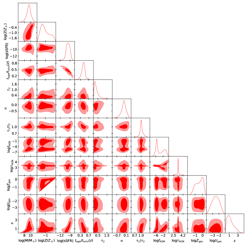
Figure 3: 1- and 2-d marginals of the SPS parameters, predicted by our galaxy population model. SPS parameters shown comprise (see also Table 1): stellar mass $(M/M_{\odot})$ and metallicity $(Z/Z_{\odot})$; specific star-formation rate $\mathrm{sSFR}$; mass-weighted age $t_{\mathrm{age}}/t_{\mathrm{univ}}(z)$, optical depths of the diffuse ($\tau_{2}$) and birth-cloud ($\tau_{1}$) dust screens; the index of the dust-attenuation law $n$ (relative to Calzetti et al., 2000); the fraction of the bolometric luminosity from AGN $f_{\mathrm{AGN}}$; the optical depth of the AGN torus $\tau_{\mathrm{AGN}}$; the gas metallicity and ionization parameter $Z_{\mathrm{gas}}$ and $U_{\mathrm{gas}}$; and redshift $z$. The star-formation rate and age are derived quantities; we assume a non-parametric (piecewise-constant) model for the SFH (see § 3.3).

In this section we present the key results from our fitted forward model. Our model predictions in data-space are validated against the COSMOS sample in §5.1, and the fitted values of the calibration-model parameters (zero-points and emission-line corrections) are given in Table 2. While most of the emission-line corrections are at the percent level or less, ten of the included bands get $\gtrsim 10\%$ or more (and up to $50\%$ in some cases). We report that emission-line calibration was essential to obtain physically reasonable population-model constraints on the fundamental-metallicity relation (gas-metallicity vs. SFR; Figure 11), and AGN (Figure 3).

The 1- and 2-d marginals for the fitted population-model are summarized in Figure 3. Since we assumed a flexible parameterization for the population model, it is designed to capture the complete web of complex dependencies between galaxy characteristics and how those evolve over cosmic time. While some of this structure is already visible in Figure 3, we present our model predictions in light of commonly studied relationships and quantities in §5.2-5.8: the redshift distribution §5.2; mass-function §5.3; mass-metallicity and fundamental relations §5.5-5.6; dust versus mass and SFR §5.7; and gas ionization versus SFR §5.8. Constraints on AGN are briefly discussed in §5.9. Note that while our model corrects for selection effects, our flexible population-model parameterization is not designed to extrapolate far below the flux-limit of the sample (where the data has no constraining power): this leads to the apparent turnover at low masses (high redshifts) in Figure 3.

Direct quantitative comparison with previous work for the relations presented in §5.2-5.8 is not always straightforward. This work represents the first time it has been possible to jointly infer the full set of galaxy parameter dependencies, while accounting for SPS-parameter degeneracies, self-calibrating the data- and calibration-model, and correcting for selection effects. It is therefore non-trivial to present like-for-like comparisons with previous studies with different SED or data-modeling assumptions, different assumed priors or specific parametric forms for scaling relations, and differing selection effects. For these reasons, in §5.2-5.8 we focus primarily on presenting a broad physical interpretation of our results, with qualitative comparison to the (most-comparable) literature where appropriate, and to template-based parameter estimates in some cases as a sanity check. We leave detailed comparison with the literature and implications for galaxy evolution to future work.

5.1 Data-space comparisons

Comparisons of our fitted model predictions to the COSMOS data in magnitude- and color-space are shown in Figures 4–6. To ensure a like-for-like comparison, Figures 4–6 compare our model predicted distributions for noisy, calibrated ($r<25$ selected) photometry against the equivalent COSMOS data. We focus on a subset of key bands and colors, spanning the full wavelength range and key color-space features, following Weaver et al. (2022).

Our model achieves excellent agreement in the magnitude marginals (Figure 4); this is not unexpected, since the magnitude marginals are mostly dominated by the shape of the mass function and volume effects, which should be easily-captured by the model.

The predictive distribution of galaxy colors on the other hand is a rich probe of galaxy evolution physics. The ability of our model to faithfully reproduce the color-color distribution underpins our confidence in the model predictions, and accurate characterization of galaxy colors as a function of redshift is crucial for predicting redshift distributions for cosmological analyses (e.g. Alsing et al., 2023). In Figures 5 and 6 we see that our model reliably reproduces the color-color distributions of COSMOS galaxies, including fine structure (e.g. related to star-forming and quiescent concentrations).

The largest discrepancies (at the level of $0.05-0.1$ magnitude color offsets) are seen in ($K_{s}-\texttt{irac1}$) and ($g-r$). These small biases are likely explained by residual (un-modeled) systematics in the COSMOS data. Weaver et al. (2022) performed a detailed comparison of the Farmer and Classic versions of the COSMOS catalogs, with different approaches to the photometric extraction. They reported the largest unexplained systematic differences between the two catalogs’ photometry in the irac1, $g$ and $u$ bands (figure 8 of Weaver et al., 2022), with ($K_{s}-\texttt{irac1}$), ($g-r$) and ($z-J$) being the most affected colors (figure 9 of Weaver et al., 2022). Discrepancies between our model predictions and the Farmer data are less than the systematic differences between Farmer and Classic in all bands and colors. It is therefore likely that any modest differences between model and data seen in Figures 5 and 6 are dominated by residual systematics in the COSMOS photometry. This makes a strong case for pursuing further improvements to the photometric data-modeling and extraction for COSMOS data in future.

In a companion paper (Thorp et al., in prep.), we will present further validation of our calibrated model in data-space, based on quantile–quantile (QQ) and probability–probability (PP) plotting.

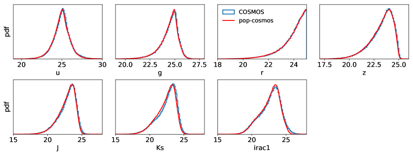
Figure 4: Comparison of the marginal distributions for the magnitudes predicted by our model (red), versus the COSMOS data (blue). Comparison is shown in the observed data-space, i.e., for $r<25$ selected galaxies and with photometric noise and calibration included (to ensure like-for-like comparison with the data). We show a subset of the $26$ bands, spanning the full wavelength range.

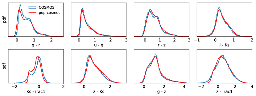
Figure 5: Comparison of the marginal color distributions predicted by our model (red), versus the COSMOS data (blue). Comparison is shown in the observed data-space, i.e., for $r<25$ selected galaxies and with photometric noise and calibration included (to ensure like-for-like comparison with the data). We show a subset of key colors following Weaver et al. (2022).

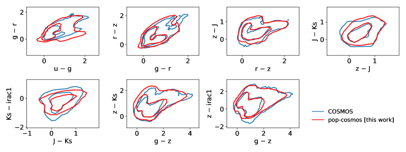
Figure 6: Color-color diagrams comparing the COSMOS data (blue) to predictions from our trained forward model (red), in the observed data-space (i.e., with photometric noise and calibration included in the model predictions to ensure like-for-like comparison with the data). Contours show 68 and 95 per cent levels. We show a subset of key colors following Weaver et al. (2022).

5.2 Redshift distribution

Accurate prediction of the redshift distributions for ensembles of (photometrically-selected) galaxies is of critical importance in constraining cosmology from weak lensing surveys (see e.g., Newman & Gruen, 2022 for a review). Redshift distributions are a key ingredient in predicting lensing and clustering statistics from data, and have significant degeneracies with key cosmological parameters of interest. This leads to very stringent requirements on their accuracy; for imminent Stage IV surveys such as LSST (Abell et al., 2009), biases on inferred redshift distributions must not exceed $0.001(1+z)$ (in the mean redshift; Mandelbaum et al., 2018).

Forward modeling has emerged as a promising avenue for obtaining accurate redshift distributions for deep broad-band imaging surveys, where sufficient spectroscopic calibration data are not available (Alsing et al., 2023). These approaches rely on accurate modeling of the galaxy population, with calibration to deep flux-limited samples such as COSMOS (as in this work) expected to provide key baseline constraints.

In Figure 7 we show our predicted galaxy redshift distribution $n(z)$ (given the photometric cuts described in §2), and compare to photometrically-derived redshift estimates from LePhare (Weaver et al., 2022). Cosmic variance is estimated following the recipe in Moster et al. (2011).

The predicted $n(z)$ is broadly in good agreement with the LePhare redshift estimates, with two notable discrepancies. Firstly, the LePhare redshifts exhibit an unphysical build-up of low or zero redshift galaxies. This is a commonly observed feature in template-based photo-$z$ estimation, where some fits get driven to the prior boundary at $z=0$, while the assumed redshift prior does not go to zero at the boundary to penalize them appropriately (Hildebrandt et al., 2012). Second, the LePhare redshift histogram exhibits clustering above $z>1$ over-and-above the expected clustering due to cosmic variance. This behavior is commonplace in template-based photo-$z$ methods, where redshift point estimates have a tendency to cluster around specific values (owing to the limited fidelity with which finite or interpolated template-sets can describe real galaxy SEDs). In contrast, our predicted $n(z)$ has the physically correct behavior of going to zero at $z=0$, and does not exhibit spurious structure above $z>1$. Conversely, since our generative model does not include galaxy clustering (present in the COSMOS sample at $z\lesssim 1$), our model implicitly learns the underlying (mean) $n(z)$, as desired.

We expect the calibrated pop-cosmos model to provide an improved population-model for predicting redshift distributions for cosmological surveys (Alsing et al., 2023). We will present pop-cosmos enabled redshift distribution estimation for KiDS data in a companion paper (Loureiro et. al., in prep.).

While we do not present individual galaxy redshift estimates here, our calibrated population model can also provide an improved prior for SPS-based photo-$z$ estimation. We are investigating the utility of pop-cosmos for redshift estimation for individual galaxies in a companion paper (Thorp et. al., in prep.).

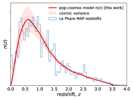
Figure 7: Photometric redshift distribution predicted by our forward model (red curve), with estimated uncertainties due to cosmic variance (red envelope). The blue histogram shows redshift estimates for COSMOS using LePhare (from Weaver et al., 2022).

5.3 Galaxy stellar mass-function

Galaxies build up stellar mass through a combination of in-situ star formation and mergers. Modeling how galaxies grow is a major ongoing challenge, involving processes that span a wide range of scales (from stellar to cosmological; see e.g., Somerville & Davé, 2015 for a review). Observations of the stellar mass function and its redshift evolution hence provide an important constraint on models of galaxy formation and evolution (Marchesini et al., 2009; Ilbert et al., 2013; Muzzin et al., 2013; Moustakas et al., 2013; Tomczak et al., 2014; Grazian et al., 2015; Song et al., 2016; Davidzon et al., 2017; Wright et al., 2018; Leja et al., 2020; Weaver et al., 2023b). In the context of photometric redshift estimation, accurate characterization of the mass function is also essential for obtaining accurate redshifts.

The stellar mass function derived from our model is shown in Figure 8. The closest study for comparison is Weaver et al. (2023b), who estimate the stellar mass function from COSMOS2020 data based on the LePhare mass estimates. To simplify the comparison (eliminating any differences in data and modeling assumptions) in Figure 8 we compare directly to the LePhare masses on which the Weaver et al. (2023b) measurement is based.

We achieve good agreement with the LePhare masses over the entire redshift range, and predict a number of key features in the mass function. We find a steepening of the low-mass slope with redshift, a buildup of galaxies around $10^{11}M_{\odot}$ below $z<1.2$ (leading to the observed “bump” in the mass function at low and intermediate redshifts), and little or no redshift dependence of the location of the knee of the mass-function. We also note relatively little evolution in the shape of the mass function at $z\lesssim 1.5$. These features are in good agreement with previous observations (including previous COSMOS analyses: Ilbert et al., 2013; Davidzon et al., 2017; Weaver et al., 2023b).

Comparison to other recent measurements such as Leja et al. (2020) are non-trivial due to differing modeling assumptions; we leave broader comparisons to future work.

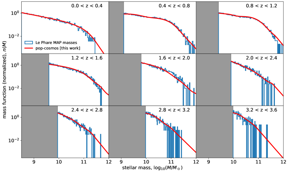
Figure 8: Predicted galaxy stellar mass functions in redshift bins of widths $\Delta z=0.4$. Our forward model predictions are shown in red, with the LePhare mass distributions shown as blue histograms. To ensure a like-for-like comparison with LePhare, we show the mass function for galaxies with an $r$-band magnitude cut $r<25$. Gray shaded regions indicate the region where the selected sample plotted begins to become incomplete (see footnote 14).

5.4 Star-forming sequence

The star-forming sequence (SFS) characterizes the relationship between star formation rate (SFR) and stellar mass, with galaxies generally forming most of their mass either on (Leitner, 2012), or passing through (Abramson et al., 2015), the star-forming sequence. Measurements of the SFS hence provide an important probe of galaxy evolution and cosmic star-formation history (Daddi et al., 2007; Noeske et al., 2007; Karim et al., 2011; Rodighiero et al., 2011; Whitaker et al., 2012, 2014; Speagle et al., 2014; Renzini & Peng, 2015; Schreiber et al., 2015; Tomczak et al., 2016; Leslie et al., 2020; Leja et al., 2022).

Figure 9 shows the inferred relationship between SFR, stellar mass, and redshift, from our population model. We compare to the measured SFS from Leja et al. (2022), which is based on COSMOS-2015 and 3D-HST photometry. This comparison is chosen because it is the most similar to our analysis; they model the SFS for star-forming and quiescent galaxies together (as in our work, rather than selecting star-forming galaxies only), the datasets used have some commonality, and the SPS modeling assumptions are similar.

Our recovered SFS is in good agreement with the measurement from Leja et al. (2022). We find a similar slope of the SFS at both low and high masses, flattening of the SFS at higher masses, steepening of the high-mass slope as a function of redshift, and a negative skewness at the high-mass end owing to the increasing presence of massive quiescent galaxies at higher masses. The small offset in normalization at low masses is mostly due to the broken power-law from Leja et al. (2022) modeling the log of the mean SFR, whereas for our model we show the median log SFR. We would also expect some modest quantitative differences due to the differing galaxy samples used, treatment of selection effects, and modeling assumptions. We note that our inferred SFS extrapolates sensibly into the regime where the COSMOS data are incomplete or lacking (Figure 9, grey bands).

The majority of observational studies have focused on characterizing the SFS for star-forming galaxies only, since those are the galaxies which are actively forming mass. However, more recently it has been shown that the method of identifying star-forming galaxies leads to systematic differences in the inferred SFS (of up to $0.5$ and $0.2$ dex in normalization and width respectively; Leja et al., 2022), owing largely to the fact that the galaxy population cannot be cleanly split into “star-forming” and “quiescent” samples based on SFR (ie., the distribution of SFR is not strongly bimodal at most masses and redshifts: see e.g., Leja et al., 2022). We emphasize that, in the spirit of Leja et al. (2022), the SFS prediction from our model presented in Figure 9 includes all galaxies in the flux-limited COSMOS sample (not only star-forming galaxies).

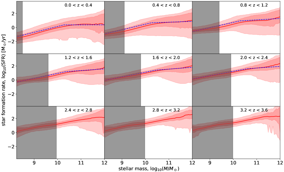
Figure 9: The star-forming sequence predicted by our forward model. The red line shows the median of our predictions of $\mathrm{log}_{10}(\mathrm{SFR})$, with the red shaded regions showing the 68 and 95% intervals of the conditional distribution at a given mass (estimated in a rolling mass window). The gray shaded region shows the estimated mass completeness limit in each redshift bin (see footnote 14). All subsequent figures follow the same plotting scheme unless noted. The blue dashed lines show the inferred SFS from Leja et al. (2022). Note that the Leja et al. (2022) predictions are for the logarithm of the mean SFR.

5.5 Mass-metallicity-redshift

The chemical enrichment of galaxies is driven by two main processes: successive generations of massive stars produce metals via nucleosynthesis and return them to the interstellar medium at the end of their lives; at the same time, outflows driven by starburst winds or AGN feedback result in ejection of metal-enriched gas into the intergalactic medium, while inflows can bring metal-poor gas in. The interplay of these processes results in a relationship between stellar mass, stellar- and gas-phase metallicities, and star-formation rate. The observed mass-metallicity and fundamental metallicity (mass-gas metallicity-SFR) relations hence provide key observational probes of galaxy evolution (Tremonti et al., 2004; Maiolino et al., 2008; Mannucci et al., 2009; Lara-López et al., 2010; Yates et al., 2012; Lara-López et al., 2013; Andrews & Martini, 2013; Nakajima & Ouchi, 2014; Yabe et al., 2015; Salim et al., 2014, 2015; Kashino et al., 2016; Cresci et al., 2019; Cullen et al., 2021; Curti et al., 2020; Bellstedt et al., 2021; Sanders et al., 2021; Thorne et al., 2022).

In Figure 10 (upper panels) we show the predicted mass-stellar metallicity relation from our population model, averaged over redshift (left panel), and as a function of redshift (right panel). The shape of the mass-metallicity relation is in excellent agreement with local measurements from SDSS at low redshift (e.g., Gallazzi et al., 2005). We find that the slope of the mass-metallicity relation at lower masses steepens by a factor of $\simeq 2$ between $z=0$ and $z=3.5$, with the trend decreasing as the mass-metallicity relation flattens off at higher masses.

In the lower panels of Figure 10 we show our population model predictions for the mass-gas metallicity relation averaged with respect to redshift (left), and as a function of redshift (right). The shape and redshift evolution is in good qualitative agreement with recent measurements (e.g., Bellstedt et al., 2021; Thorne et al., 2022). We find the slope of the mass-gas metallicity relation at lower masses steepens by a factor of $\simeq 2$ between $z=0$ and $z=3.5$, with the median gas metallicity at $10^{10}M_{\odot}$ decreasing by around $0.4$ dex over the same redshift range. This is roughly consistent with recent measurements from GAMA data (Bellstedt et al., 2020), which shows around $0.6$ dex decrease in the median gas-metallicity over a similar redshift range.

The normalization of the recovered mass-gas metallicity relation (bottom row of Figure 10) is higher than for the mass-stellar metallicity relation (top row of Figure 10). This is expected, since under our assumed SPS model the gas metallicity represents the present-day metallicity of the ISM, while the stellar-metallicity parameter is a proxy for the light-weighted average metallicity among the stellar population (which includes older stars).

Note that for both stellar and gas metallicity, in the regime where the COSMOS data is lacking (grey bands in Figure 10) the extrapolation of our model predictions show a flattening of the mass-metallicity relations, while from observations it is expected to continue downwards (e.g., Kirby et al., 2013). Our model is not designed to extrapolate very far into the regime where the data is lacking; additional constraints may be needed to improve the extrapolation of the mass-metallicity relations at low masses, if desired.

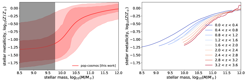
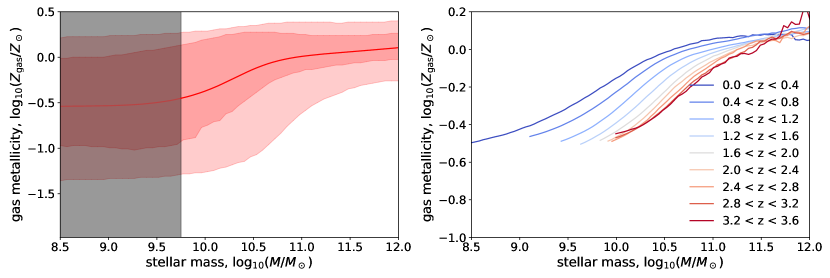
Figure 10: Upper left panel: predicted stellar metallicity vs. mass relation. Upper right panel: median predicted mass–metallicity relation in redshift bins of width $\Delta z=0.4$. Lower left and right panels are the same, but for gas metallicity. Grey bands indicate where the COSMOS sample becomes incomplete (see footnote 14).

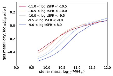
Figure 11: Fundamental metallicity relation showing median predicted gas metallicity conditional on stellar mass in bins of $\mathrm{log}_{10}(\mathrm{sSFR})$.

5.6 Fundamental metallicity relation

The interplay between star formation and the chemical enrichment of the ISM is expected to result in a relationship between mass, gas-phase metallicity, and star-formation rate – the so-called fundamental metallicity relation (FMR; Mannucci et al., 2010; Dayal et al., 2013).

In Figure 11 we show the dependence of the mass-gas metallicity relation with SFR; the second component of the fundamental metallicity relation. We find a clear and smooth negative trend between gas metallicity and SFR for masses up to around $10^{11.5}M_{\odot}$, with a $0.2-0.3$ dex evolution in the median gas metallicity across the full dynamic range of SFR, across most stellar masses. This is qualitatively consistent with other measurements in the literature (Mannucci et al., 2010; Dayal et al., 2013; Salim et al., 2014; Zahid et al., 2014; Curti et al., 2020; Thorne et al., 2022), and sits roughly in the middle in terms of the magnitude of the trend compared to recent measurements (e.g., Curti et al., 2020 find a trend of up to $0.5$ dex, while Thorne et al., 2022 report an overall variation of only $0.13$ dex with SFR).

Whether or not there exists a dependence of the mass-gas metallicity relation with SFR at all (and hence the existence of the FMR as a fundamental plane) is still under debate, with some studies finding a negative trend between gas-metallicity and SFR (Mannucci et al., 2010; Dayal et al., 2013; Salim et al., 2014; Zahid et al., 2014; Curti et al., 2020; Thorne et al., 2022), while others report no significant correlation (Sánchez et al., 2013, 2017, 2019) or even a positive trend (Lara-López et al., 2013). Nevertheless, our measurement of the FMR is qualitatively consistent with the most recent measurements (Curti et al., 2020; Thorne et al., 2022), and with the physical expectation of a negative trend between gas-metallicity and SFR (Mannucci et al., 2010; Dayal et al., 2013).

We report that inclusion of the gas ionization parameter in our SPS model was essential to recover reasonable inferences about gas-metallicity: without $\mathrm{log}\,U_{\mathrm{gas}}$, our population-model was unable to recover physically sound predictions for mass-gas metallicity relation and FMR.

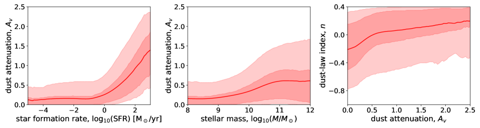
Figure 12: Left panel: predicted diffuse dust attenuation as a function of SFR (left) and stellar mass (middle), and the index of the dust attenuation law as a function of dust attenuation (right).

5.7 Dust attenuation

The microscopic properties of dust grains (e.g. size, material, etc.) govern their interaction with light, and the direct impact this has on a galaxy’s SED (see e.g., Calzetti, 2001 or Draine, 2003 for a review). Dust grains also impact SEDs through their key role in galaxy star formation, as their surfaces act as favorable media for the formation of molecular hydrogen (Gould & Salpeter, 1963; Hollenbach & Salpeter, 1971). Dust also serves as a key component in regulating heating and cooling, further affecting the star formation cycle (Yamasawa et al., 2011). Observations of how dust properties relate to other galaxy characteristics are important in constraining models of galaxy evolution, with key observational targets including the degeneracy between attenuation slope and optical depth, star-dust geometry, and correlations between dust properties with mass and star formation rate (e.g. Burgarella et al., 2005; Noll et al., 2009; Garn & Best, 2010; Buat et al., 2012; Zahid et al., 2013; Kriek & Conroy, 2013; Chevallard et al., 2013; Reddy et al., 2015; Salim et al., 2016; Salmon et al., 2016; Leja et al., 2017; Salim et al., 2018; Salim & Boquien, 2019; Nagaraj et al., 2022; Lower et al., 2022, 2023).

Figure 12 (left panel) shows our inferred relationship between (diffuse) dust attenuation and SFR. We see that quiescent galaxies have a tendency toward little or no dust attenuation, although a tail out to non-negligible dust contributions for quiescent galaxies is present. For $\mathrm{log}_{10}(\text{SFR})\gtrsim 0$ the typical level of dust attenuation increases and the spread broadens. Studies of SDSS star-forming galaxies (using H-$\alpha$ emission or the Balmer decrement to measure attenuation, Garn & Best, 2010; Zahid et al., 2013, e.g.) show very similar behavior, with dust attenuation picking up around $\mathrm{log}_{10}(\text{SFR})\gtrsim 0$. More recently, a photometric analysis by Nagaraj et al. (2022) using 3D-HST data and the Prospector SPS model also found a strong increase in optical depth at $\mathrm{log}_{10}(\text{SFR})\gtrsim 0$, very similar to our results.

The relationship between dust attenuation and stellar mass (Figure 12, middle panel) shows a broadening and increase in dust attenuation for galaxies $\gtrsim 10^{10}M_{\odot}$. Nagaraj et al. (2022) also find a similar relationship between dust attenuation and stellar mass, where galaxies $\gtrsim 10^{10}M_{\odot}$ have higher dust attenuation on average (by around a factor of two) compared to those $\lesssim 10^{10}M_{\odot}$. Similar results are found by Salim et al. (2018), who identify a tendency for higher attenuation values (and a larger scatter) to be seen for more massive galaxies. Our result is also consistent with previous studies of SN Ia host galaxies, where the distribution of extinction values is typically observed to be broader (longer tailed) in galaxies $\gtrsim 10^{10}M_{\odot}$ (e.g. Sullivan et al., 2010; Childress et al., 2013; Thorp et al., 2021; Meldorf et al., 2023; Grayling et al., 2024).

In Figure 12 (right panel), we show our inferred relation between dust law index and dust attenuation (for the diffuse dust component). We see a trend towards higher $n$ (shallower attenuation law) for galaxies with higher levels of attenuation, with substantial dispersion ($\sim 0.3$) of the dust index $n$ for any given attenuation $A_{V}$. This is qualitatively consistent with recent literature (Buat et al., 2012; Kriek & Conroy, 2013; Reddy et al., 2015; Salim et al., 2018; Álvarez-Márquez et al., 2019; Battisti et al., 2020; Nagaraj et al., 2022), and with expectations from radiative transfer calculations (e.g. Witt & Gordon, 2000; Chevallard et al., 2013). We leave an extended quantitative comparison with previous literature to future work.

5.8 Gas physics

While the detailed connection between gas dynamics and star formation is non-trivial, one clear expectation is that gas ionization will increase with increased star formation activity, with massive young stars contributing heavily to the ionizing photon budget. Our population model predicts a clear increasing trend in gas ionization with specific star formation rate (Figure 13), qualitatively consistent with previous studies (eg., Kaasinen et al., 2018) and in line with physical expectations. The slope and normalization from Kaasinen et al. (2018) differ somewhat from our model. We expect relatively weak constraints expected on gas ionization from photometry alone, with emission-lines typically contributing a few percent at most to broad-band fluxes; the level of agreement with Kaasinen et al. (2018) is very reasonable given the limitations of photometric observations. It is also possible that some differences are due to selection effects in the Kaasinen et al. (2018) sample.

5.9 Active galaxies

Figure 3 shows some structure in our calibrated population model between AGN and other SPS parameters; most notably, a tendency for the brightest AGN (higher $f_{\mathrm{AGN}}$) to be redder (higher $\tau_{\mathrm{AGN}}$), in line with physical expectations. We note that the sharp peak at low values of $f_{\mathrm{AGN}}$ (and the corresponding spike at intermediate values of $\tau_{\mathrm{AGN}}$) is an artefact of how we perform the population-model fits, and the information content of the data. For the portion of the galaxy population with little or no AGN contribution, there are no AGN constraints from the data and hence nothing to prefer a sharp peak at some negligible value of $f_{\mathrm{AGN}}$ over any other distribution over very low values of $f_{\mathrm{AGN}}$: neither have any discernible impact on the model predictions. Similarly there are no meaningful constraints on $\tau_{\mathrm{AGN}}$ for galaxies with no AGN contribution; the fact that our model gives all the galaxies with no AGN intermediate values of $\tau_{\mathrm{AGN}}$ has no impact on our model predictions. While inclusion of AGN is important for population-modeling, drawing detailed inferences about AGN physics likely requires a more sophisticated parameterization of the AGN contribution to the galaxy SEDs.

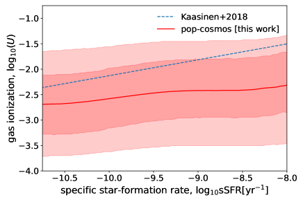
Figure 13: Predicted dependence of gas ionization on sSFR. The blue line shows the relation from Kaasinen et al. (2018).

6 Discussion

The pop-cosmos population model presented in §5 is calibrated down to an $r$-band magnitude of $r<25$. Since selection effects are corrected for, we expect the model predictions to be valid slightly deeper than $r<25$, becoming less reliable into the fainter regime where the data is lacking. One of the primary use-cases of our population model in a cosmological inference context is for predicting galaxy redshift distributions from deep, broad-band data from Stage IV surveys such as LSST (Alsing et al., 2023). The gold sample for LSST is expected to have a limiting magnitude $r<25.3$, only $0.3$ magnitudes deeper than the COSMOS sample used in this work. Care will need to be taken in examining the extent to which pop-cosmos can extrapolate to $r<25.3$; we leave this to future work. As a stepping-stone to Stage IV cosmological survey applications, we will present pop-cosmos enabled redshift distribution estimation for Stage III (KiDS) data in a companion paper (Loureiro et. al., in prep.), as well as the utility of pop-cosmos as an improved model and prior for individual galaxy photo-$z$ estimation (Thorp et. al., in prep.).

In the context of calibrating an accurate galaxy population model for improving cosmological analyses (e.g., Alsing et al., 2023; Moser et al., 2024), the galaxy-evolution results presented in §5 are a essentially side-effect of pursuing accurate redshifts. Nonetheless, the advancement in methodology means that many of the inferred scaling relations may be better measured by our new framework.

Measurement of the FMR, mass-metallicity-redshift and sSFR-gas ionization relations has generally been considered challenging or impossible from photometric data alone. Nonetheless, in §5.5-5.8 we present measurements of these relations that are qualitatively consistent with previous results (from spectroscopic data). This opens up an exciting new approach to measuring these quantities, which merits further investigation. Even where our predictions about gas-phase physics do not agree in detail with spectroscopic measurements (likely due to the limitations of photometric data), we do not expect this to have a significant effect on the photometric redshift program: corrections to broad-band photometry should be tiny.

In §5.1 we saw that our model predictions for galaxy colors are accurate to within observed calibration biases between different photometric extraction methods (e.g., the Farmer vs. Classic versions of the COSMOS photometry; Weaver et al., 2023a). There is hence no evidence that additional complexity in the SPS model is justified at this stage to improve the population-model predictions. Nevertheless, the scalability of our simulation-based inference approach opens up the possibility of including further extensions (and parameters) within the SPS model, while remaining computationally feasible.

We established that self-calibration of emission-line corrections was important for drawing reasonable population-level predictions of the fundamental metallicity relation and AGN, and was shown to improve photometric redshift inferences in the COSMOS data (see, e.g., Alarcon et al. 2021; Leistedt et al. 2023). While parameterizing the mean bias in the most important emission-lines captures the leading order correction, in practice emission line strengths will be a strong function of the SPS parameters. It would be straightforward to incorporate parameter-dependent emission-line corrections in our calibration model; we leave this to future work.

Recently, another forward modeling-based approach to inferring the population distribution of galaxy parameters has been presented(popsed; Li et al., 2024), also making use of the OT distance as an objective function in their inference procedure. They use normalizing flows as their population distribution over SPS parameters, with a 12-parameter SPS model following Hahn et al. (2023), and an SPS emulation scheme similar to Alsing et al. (2020). They demonstrate the method on broad-band SDSS $ugriz$ photometry for a sample of galaxies from the Galaxies and Mass Assembly survey (GAMA; Driver et al., 2011; Baldry et al., 2018), with a depth of $r<19.8$ and at relatively low redshift $z\lesssim 0.45$, showing in particular that they can recover the star-forming main sequence (c.f. our §5.4 and Figure 9).

Our work goes further than Li et al. (2024) by constructing and fitting a comprehensive forward model for the data, including: a flexible population-model; state-of-the-art (16-parameter) SED model; self-calibration of the data-modeling (noise and calibration); and explicit treatment of selection effects. By utilizing a larger, deeper galaxy sample, we cover the depth ($r<25$) and redshift range ($z\lesssim 3.5$) required for modeling Stage III and IV wide-deep galaxy surveys. The broad wavelength range covered by the $26$-bands used here (including intermediate and narrow bands) also allows us to constrain a comprehensive range of galaxy evolution physics, for a diverse galaxy sample. As a result our calibrated population-model can faithfully predict galaxy colors over a wide range of wavelengths and redshifts, with direct utility in a cosmological inference context for Stage III and IV surveys.

Another forward modeling-based approach has been developed by Moser et al. (2024) and applied to image-level data from HSC (Aihara et al., 2022). Their population model is parametric, with galaxy spectra built up from Kcorrect templates (Blanton et al., 2017), and source detection within their simulated images being handled by SExtractor (Bertin & Arnouts, 1996). Their inference is carried out using an approximate Bayesian computation (ABC) scheme (also employed by Tortorelli et al., 2020, 2021). Our work differs from theirs in utilizing a continuous SPS model (rather than templates) for galaxy SEDs, and a flexible (diffusion-model) parameterization of the population-model, while jointly calibrating the population- and data-model simultaneously. OT optimization is also expected to scale favourably to high-dimensional problems on large datasets, where ABC quickly becomes computationally infeasible due to the high number of simulations required (see e.g., Alsing et al., 2019). Nevertheless, forward modeling at the level of images represents an important advance, and may be necessary for including image-based selection effects in future analyses.

7 Conclusions

We have presented pop-cosmos: a comprehensive population model fit to a large, deep, flux-limited sample of galaxies from COSMOS. We constructed a detailed forward model for the COSMOS data, including a flexible diffusion-model parameterzation of the population-distribution of galaxy characteristics, a state-of-the-art (16-parameter) SPS model, and a detailed data-model describing the observation, calibration and selection processes. By comparing synthetic and real data in a simulation-based inference setting, we were able to jointly fit the population-model while self-calibrating the data- and calibration-model parameters in a self-consistent fashion. As a result, we obtained a robustly calibrated population model describing galaxies down to $r<25$ and out to redshift $z\simeq 3.5$.

Our population model is able to faithfully reproduce galaxy colors (to within the limitations of the photometric calibration of the COSMOS data), and encodes a comprehensive and compelling picture of galaxy evolution processes. This represents the first time that it has been possible to jointly infer the full, complex web of dependencies between galaxy characteristics, together with the photometric noise, data- and model-calibration, and de-convolution of selection effects: a key milestone in the analysis of large galaxy surveys.

Accurate galaxy population models calibrated to large, deep, narrow band (or spectroscopic) data are of key importance in drawing robust cosmological measurements from galaxy surveys. We expect the pop-cosmos model and its successors to open up new capabilities in accurate redshift estimation from photometric data, eliminating systematics in transient cosmology due to correlations between host galaxy properties and supernovae, and in modeling and inferring the galaxy-halo connection.

References

- Abbott et al. (2019) Abbott, T. M. C., Abdalla, F. B., Alarcon, A., et al. 2019, Phys. Rev. D, 100, 023541
- Abell et al. (2009) Abell, P. A., Allison, J., Anderson, S. F., et al. 2009, arXiv e-prints, arXiv:0912.0201
- Abramson et al. (2015) Abramson, L. E., Gladders, M. D., Dressler, A., et al. 2015, ApJ, 801, L12
- Aihara et al. (2018) Aihara, H., Armstrong, R., Bickerton, S., et al. 2018, PASP, 70, S8
- Aihara et al. (2022) Aihara, H., AlSayyad, Y., Ando, M., et al. 2022, PASJ, 74, 247
- Alarcon et al. (2021) Alarcon, A., Gaztanaga, E., Eriksen, M., et al. 2021, MNRAS, 501, 6103
- Alsing et al. (2019) Alsing, J., Charnock, T., Feeney, S., & Wandelt, B. 2019, MNRAS, 488, 4440
- Alsing et al. (2023) Alsing, J., Peiris, H., Mortlock, D., Leja, J., & Leistedt, B. 2023, ApJS, 264, 29
- Alsing et al. (2020) Alsing, J., Peiris, H., Leja, J., et al. 2020, ApJS, 249, 5
- Altschuler et al. (2017) Altschuler, J., Niles-Weed, J., & Rigollet, P. 2017, in Advances in Neural Information Processing Systems, ed. I. Guyon, U. V. Luxburg, S. Bengio, H. Wallach, R. Fergus, S. Vishwanathan, & R. Garnett, Vol. 30 (Curran Associates, Inc.)
- Álvarez-Márquez et al. (2019) Álvarez-Márquez, J., Burgarella, D., Buat, V., Ilbert, O., & Pérez-González, P. G. 2019, A&A, 630, A153
- Anderson (1982) Anderson, B. D. 1982, Stochastic Processes and their Applications, 12, 313
- Andrews & Martini (2013) Andrews, B. H., & Martini, P. 2013, ApJ, 765, 140
- Arnouts et al. (1999) Arnouts, S., Cristiani, S., Moscardini, L., et al. 1999, MNRAS, 310, 540
- Arnouts et al. (2013) Arnouts, S., Le Floc’h, E., Chevallard, J., et al. 2013, A&A, 558, A67
- Baldry et al. (2018) Baldry, I. K., Liske, J., Brown, M. J. I., et al. 2018, MNRAS, 474, 3875
- Battisti et al. (2020) Battisti, A., Da Cunha, E., Shivaei, I., et al. 2020, ApJ, 888, 108
- Bellstedt et al. (2020) Bellstedt, S., Robotham, A. S., Driver, S. P., et al. 2020, MNRAS, 498, 5581
- Bellstedt et al. (2021) Bellstedt, S., Robotham, A. S. G., Driver, S. P., et al. 2021, MNRAS, 503, 3309
- Benitez (2000) Benitez, N. 2000, ApJ, 536, 571
- Bertin & Arnouts (1996) Bertin, E., & Arnouts, S. 1996, A&AS, 117, 393
- Bishop (2006) Bishop, C. M. 2006, Pattern Recognition and Machine Learning (Springer)
- Blanton et al. (2017) Blanton, M. R., Bershady, M. A., Abolfathi, B., et al. 2017, AJ, 154, 28
- Brammer et al. (2008) Brammer, G. B., van Dokkum, P. G., & Coppi, P. 2008, ApJ, 686, 1503
- Briday et al. (2022) Briday, M., Rigault, M., Graziani, R., et al. 2022, A&A, 657, A22
- Brout & Scolnic (2021) Brout, D., & Scolnic, D. 2021, ApJ, 909, 26
- Buat et al. (2012) Buat, V., Noll, S., Burgarella, D., et al. 2012, A&A, 545, A141
- Burgarella et al. (2005) Burgarella, D., Buat, V., & Iglesias-Paramo, J. 2005, MNRAS, 360, 1413
- Byler et al. (2017) Byler, N., Dalcanton, J. J., Conroy, C., & Johnson, B. D. 2017, ApJ, 840, 44
- Calzetti (2001) Calzetti, D. 2001, PASP, 113, 1449
- Calzetti et al. (2000) Calzetti, D., Armus, L., Bohlin, R. C., et al. 2000, ApJ, 533, 682
- Charlier et al. (2021) Charlier, B., Feydy, J., Glaunès, J. A., Collin, F.-D., & Durif, G. 2021, J. Machine Learning Res., 22, 1
- Charlot & Fall (2000) Charlot, S., & Fall, S. M. 2000, ApJ, 539, 718
- Chen et al. (2018) Chen, R. T. Q., Rubanova, Y., Bettencourt, J., & Duvenaud, D. K. 2018, in Advances in Neural Information Processing Systems, ed. S. Bengio, H. Wallach, H. Larochelle, K. Grauman, N. Cesa-Bianchi, & R. Garnett, Vol. 31 (Curran Associates, Inc.)
- Chevallard et al. (2013) Chevallard, J., Charlot, S., Wandelt, B., & Wild, V. 2013, MNRAS, 432, 2061
- Childress et al. (2013) Childress, M., Aldering, G., Antilogus, P., et al. 2013, ApJ, 770, 108
- Childress et al. (2014) Childress, M. J., Wolf, C., & Zahid, H. J. 2014, MNRAS, 445, 1898
- Conroy (2013) Conroy, C. 2013, ARA&A, 51, 393
- Conroy & Gunn (2010a) Conroy, C., & Gunn, J. E. 2010a, ApJ, 712, 833
- Conroy & Gunn (2010b) —. 2010b, Astrophysics Source Code Library, record ascl:1010.043
- Conroy et al. (2009) Conroy, C., Gunn, J. E., & White, M. 2009, ApJ, 699, 486
- Conroy et al. (2010) Conroy, C., White, M., & Gunn, J. E. 2010, ApJ, 708, 58
- Cresci et al. (2019) Cresci, G., Mannucci, F., & Curti, M. 2019, A&A, 627, A42
- Cullen et al. (2021) Cullen, F., Shapley, A., McLure, R., et al. 2021, MNRAS, 505, 903
- Curti et al. (2020) Curti, M., Mannucci, F., Cresci, G., & Maiolino, R. 2020, MNRAS, 491, 944
- Cuturi (2013) Cuturi, M. 2013, in Advances in Neural Information Processing Systems, ed. C. Burges, L. Bottou, M. Welling, Z. Ghahramani, & K. Weinberger, Vol. 26 (Curran Associates, Inc.)
- Daddi et al. (2007) Daddi, E., Dickinson, M., Morrison, G., et al. 2007, ApJ, 670, 156
- Davidzon et al. (2017) Davidzon, I., Ilbert, O., Laigle, C., et al. 2017, A&A, 605, A70
- Dayal et al. (2013) Dayal, P., Ferrara, A., & Dunlop, J. S. 2013, MNRAS, 430, 2891
- De Jong et al. (2015) De Jong, J. T., Kleijn, G. A. V., Boxhoorn, D. R., et al. 2015, A&A, 582, A62
- Dinh et al. (2016) Dinh, L., Sohl-Dickstein, J., & Bengio, S. 2016, arXiv e-prints, arXiv:1605.08803
- Draine (2003) Draine, B. T. 2003, ARA&A, 41, 241
- Driver et al. (2011) Driver, S. P., Hill, D. T., Kelvin, L. S., et al. 2011, MNRAS, 413, 971
- Duarte et al. (2023) Duarte, J., González-Gaitán, S., Mourão, A., et al. 2023, A&A, 680, A56
- Durkan et al. (2019) Durkan, C., Bekasov, A., Murray, I., & Papamakarios, G. 2019, in Advances in Neural Information Processing Systems, ed. H. Wallach, H. Larochelle, A. Beygelzimer, F. d'Alché-Buc, E. Fox, & R. Garnett, Vol. 32 (Curran Associates, Inc.)
- Dvurechensky et al. (2018) Dvurechensky, P., Gasnikov, A., & Kroshnin, A. 2018, in Proc. Machine Learning Res., Vol. 80, Proceedings of the 35th International Conference on Machine Learning, ed. J. Dy & A. Krause (PMLR), 1367–1376
- Eadie et al. (2023) Eadie, G. M., Speagle, J. S., Cisewski-Kehe, J., et al. 2023, arXiv e-prints, arXiv:2302.04703
- Feeney et al. (2019) Feeney, S. M., Peiris, H. V., Williamson, A. R., et al. 2019, Phys. Rev. Lett., 122, 061105
- Ferland et al. (2013) Ferland, G. J., Porter, R. L., van Hoof, P. A. M., et al. 2013, Rev. Mexicana Astron. Astrofis., 49, 137
- Ferland et al. (2017) Ferland, G. J., Chatzikos, M., Guzmán, F., et al. 2017, Rev. Mexicana Astron. Astrofis., 53, 385
- Feydy et al. (2019) Feydy, J., Séjourné, T., Vialard, F.-X., et al. 2019, in Proc. Machine Learning Res., Vol. 89, Proceedings of the Twenty-Second International Conference on Artificial Intelligence and Statistics, ed. K. Chaudhuri & M. Sugiyama (PMLR), 2681–2690
- Flaugher (2005) Flaugher, B. 2005, Inter. J. Modern Phys. A, 20, 3121
- Foley & Mandel (2013) Foley, R. J., & Mandel, K. 2013, ApJ, 778, 167
- Foreman-Mackey et al. (2014) Foreman-Mackey, D., Sick, J., & Johnson, B. 2014, python-fsps: Python bindings to FSPS (v0.1.1), doi: 10.5281/zenodo.12157
- Gagliano et al. (2023) Gagliano, A., Contardo, G., Foreman-Mackey, D., Malz, A. I., & Aleo, P. D. 2023, ApJ, 954, 6
- Gagliano et al. (2021) Gagliano, A., Narayan, G., Engel, A., Carrasco Kind, M., & LSST Dark Energy Science Collaboration. 2021, ApJ, 908, 170
- Gallazzi et al. (2005) Gallazzi, A., Charlot, S., Brinchmann, J., White, S. D. M., & Tremonti, C. A. 2005, MNRAS, 362, 41
- Garn & Best (2010) Garn, T., & Best, P. N. 2010, MNRAS, 409, 421
- Germain et al. (2015) Germain, M., Gregor, K., Murray, I., & Larochelle, H. 2015, in Proc. Machine Learning Res., Vol. 37, Proceedings of the 32nd International Conference on Machine Learning, ed. F. Bach & D. Blei (Lille, France: PMLR), 881–889
- Gould & Salpeter (1963) Gould, R. J., & Salpeter, E. E. 1963, ApJ, 138, 393
- Grathwohl et al. (2018) Grathwohl, W., Chen, R. T., Bettencourt, J., Sutskever, I., & Duvenaud, D. 2018, arXiv e-prints, arXiv:1810.01367
- Grayling et al. (2024) Grayling, M., Thorp, S., Mandel, K. S., et al. 2024, arXiv e-prints, arXiv:2401.08755
- Grazian et al. (2015) Grazian, A., Fontana, A., Santini, P., et al. 2015, A&A, 575, A96
- Guzmán et al. (2017) Guzmán, F., Badnell, N. R., Williams, R. J. R., et al. 2017, MNRAS, 464, 312
- Hahn et al. (2023) Hahn, C., Kwon, K. J., Tojeiro, R., et al. 2023, ApJ, 945, 16
- Hasinger et al. (2018) Hasinger, G., Capak, P., Salvato, M., et al. 2018, ApJ, 858, 77
- Hildebrandt et al. (2012) Hildebrandt, H., Erben, T., Kuijken, K., et al. 2012, MNRAS, 421, 2355
- Ho et al. (2020) Ho, J., Jain, A., & Abbeel, P. 2020, in Advances in Neural Information Processing Systems, ed. H. Larochelle, M. Ranzato, R. Hadsell, M. Balcan, & H. Lin, Vol. 33 (Curran Associates, Inc.), 6840–6851
- Hollenbach & Salpeter (1971) Hollenbach, D., & Salpeter, E. E. 1971, ApJ, 163, 155
- Hyvärinen (2005) Hyvärinen, A. 2005, J. Machine Learning Res., 6, 695
- Ilbert et al. (2006) Ilbert, O., Arnouts, S., McCracken, H., et al. 2006, A&A, 457, 841
- Ilbert et al. (2013) Ilbert, O., McCracken, H. J., Le Fèvre, O., et al. 2013, A&A, 556, A55
- Kaasinen et al. (2018) Kaasinen, M., Kewley, L., Bian, F., et al. 2018, MNRAS, 477, 5568
- Kantorovich & Rubinstein (1958) Kantorovich, L., & Rubinstein, G. S. 1958, Vestnik Leningrad Univ., 13, 52
- Karim et al. (2011) Karim, A., Schinnerer, E., Martínez-Sansigre, A., et al. 2011, ApJ, 730, 61
- Kashino et al. (2016) Kashino, D., Renzini, A., Silverman, J., & Daddi, E. 2016, ApJ, 823, L24
- Kelly et al. (2010) Kelly, P. L., Hicken, M., Burke, D. L., Mandel, K. S., & Kirshner, R. P. 2010, ApJ, 715, 743
- Kewley & Ellison (2008) Kewley, L. J., & Ellison, S. L. 2008, ApJ, 681, 1183
- Kingma et al. (2021) Kingma, D., Salimans, T., Poole, B., & Ho, J. 2021, in Advances in Neural Information Processing Systems, ed. M. Ranzato, A. Beygelzimer, Y. Dauphin, P. Liang, & J. W. Vaughan, Vol. 34 (Curran Associates, Inc.), 21696–21707
- Kingma & Ba (2014) Kingma, D. P., & Ba, J. 2014, arXiv e-prints, arXiv:1412.6980
- Kingma & Dhariwal (2018) Kingma, D. P., & Dhariwal, P. 2018, in Advances in Neural Information Processing Systems, ed. S. Bengio, H. Wallach, H. Larochelle, K. Grauman, N. Cesa-Bianchi, & R. Garnett, Vol. 31 (Curran Associates, Inc.)
- Kingma & Welling (2013) Kingma, D. P., & Welling, M. 2013, arXiv preprint arXiv:1312.6114
- Kirby et al. (2013) Kirby, E. N., Cohen, J. G., Guhathakurta, P., et al. 2013, The Astrophysical Journal, 779, 102
- Kriek & Conroy (2013) Kriek, M., & Conroy, C. 2013, ApJ, 775, L16
- Kullback & Leibler (1951) Kullback, S., & Leibler, R. A. 1951, Ann. Math. Statistics, 22, 79
- Kwon et al. (2022) Kwon, D., Fan, Y., & Lee, K. 2022, in Advances in Neural Information Processing Systems, ed. S. Koyejo, S. Mohamed, A. Agarwal, D. Belgrave, K. Cho, & A. Oh, Vol. 35 (Curran Associates, Inc.), 20205–20217
- Lara-López et al. (2010) Lara-López, M., Cepa, J., Bongiovanni, A., et al. 2010, A&A, 521, L53
- Lara-López et al. (2013) Lara-López, M., Hopkins, A. M., Lopez-Sanchez, A. R., et al. 2013, MNRAS, 434, 451
- Laureijs et al. (2011) Laureijs, R., Amiaux, J., Arduini, S., et al. 2011, arXiv e-prints, arXiv:1110.3193
- Leistedt et al. (2023) Leistedt, B., Alsing, J., Peiris, H., Mortlock, D., & Leja, J. 2023, ApJS, 264, 23
- Leitner (2012) Leitner, S. N. 2012, ApJ, 745, 149
- Leja et al. (2019a) Leja, J., Carnall, A. C., Johnson, B. D., Conroy, C., & Speagle, J. S. 2019a, ApJ, 876, 3
- Leja et al. (2018) Leja, J., Johnson, B. D., Conroy, C., & van Dokkum, P. 2018, ApJ, 854, 62
- Leja et al. (2017) Leja, J., Johnson, B. D., Conroy, C., van Dokkum, P. G., & Byler, N. 2017, ApJ, 837, 170
- Leja et al. (2020) Leja, J., Speagle, J. S., Johnson, B. D., et al. 2020, ApJ, 893, 111
- Leja et al. (2019b) Leja, J., Johnson, B. D., Conroy, C., et al. 2019b, ApJ, 877, 140
- Leja et al. (2022) Leja, J., Speagle, J. S., Ting, Y.-S., et al. 2022, ApJ, 936, 165
- Leslie et al. (2020) Leslie, S. K., Schinnerer, E., Liu, D., et al. 2020, ApJ, 899, 58
- Li et al. (2024) Li, J., Melchior, P., Hahn, C., & Huang, S. 2024, AJ, 167, 16
- Lilly et al. (2007) Lilly, S. J., Fevre, O. L., Renzini, A., et al. 2007, ApJS, 172, 70
- Lower et al. (2023) Lower, S., Narayanan, D., Hu, C.-Y., & Privon, G. C. 2023, arXiv e-prints, arXiv:2306.07338
- Lower et al. (2022) Lower, S., Narayanan, D., Leja, J., et al. 2022, ApJ, 931, 14
- Luo (2022) Luo, C. 2022, arXiv e-prints, arXiv:2208.11970
- Madau & Dickinson (2014) Madau, P., & Dickinson, M. 2014, ARA&A, 52, 415
- Maiolino et al. (2008) Maiolino, R., Nagao, T., Grazian, A., et al. 2008, A&A, 488, 463
- Mandelbaum et al. (2018) Mandelbaum, R., Eifler, T., Hložek, R., et al. 2018, arXiv e-prints, arXiv:1809.01669
- Mannucci et al. (2010) Mannucci, F., Cresci, G., Maiolino, R., Marconi, A., & Gnerucci, A. 2010, MNRAS, 408, 2115
- Mannucci et al. (2006) Mannucci, F., Della Valle, M., & Panagia, N. 2006, MNRAS, 370, 773
- Mannucci et al. (2005) Mannucci, F., Della Valle, M., Panagia, N., et al. 2005, A&A, 433, 807
- Mannucci et al. (2009) Mannucci, F., Cresci, G., Maiolino, R., et al. 2009, MNRAS, 398, 1915
- Maoutsa et al. (2020) Maoutsa, D., Reich, S., & Opper, M. 2020, Entropy, 22, 802
- Marchesini et al. (2009) Marchesini, D., Van Dokkum, P. G., Schreiber, N. M. F., et al. 2009, ApJ, 701, 1765
- Masters et al. (2017) Masters, D. C., Stern, D. K., Cohen, J. G., et al. 2017, ApJ, 841, 111
- Masters et al. (2019) —. 2019, ApJ, 877, 81
- McGill et al. (2023) McGill, P., Anderson, J., Casertano, S., et al. 2023, MNRAS, 520, 259
- Meldorf et al. (2023) Meldorf, C., Palmese, A., Brout, D., et al. 2023, MNRAS, 518, 1985
- Moser et al. (2024) Moser, B., Kacprzak, T., Fischbacher, S., et al. 2024, arXiv e-prints, arXiv:2401.06846
- Moster et al. (2011) Moster, B. P., Somerville, R. S., Newman, J. A., & Rix, H.-W. 2011, ApJ, 731, 113
- Moustakas et al. (2013) Moustakas, J., Coil, A. L., Aird, J., et al. 2013, ApJ, 767, 50
- Muzzin et al. (2013) Muzzin, A., Marchesini, D., Stefanon, M., et al. 2013, ApJS, 206, 8
- Nagaraj et al. (2022) Nagaraj, G., Forbes, J. C., Leja, J., Foreman-Mackey, D., & Hayward, C. C. 2022, ApJ, 932, 54
- Nakajima & Ouchi (2014) Nakajima, K., & Ouchi, M. 2014, MNRAS, 442, 900
- Newman & Gruen (2022) Newman, J. A., & Gruen, D. 2022, arXiv e-prints, arXiv:2206.13633
- Nicolas et al. (2021) Nicolas, N., Rigault, M., Copin, Y., et al. 2021, A&A, 649, A74
- Nixon et al. (2023) Nixon, M. C., Welbanks, L., McGill, P., & Kempton, E. M. R. 2023, arXiv e-prints, arXiv:2310.03713
- Noeske et al. (2007) Noeske, K., Weiner, B., Faber, S., et al. 2007, ApJ, 660, L43
- Noll et al. (2009) Noll, S., Burgarella, D., Giovannoli, E., et al. 2009, A&A, 507, 1793
- Papamakarios et al. (2021) Papamakarios, G., Nalisnick, E., Rezende, D. J., Mohamed, S., & Lakshminarayanan, B. 2021, J. Machine Learning Res., 22, 2617
- Papamakarios et al. (2017) Papamakarios, G., Pavlakou, T., & Murray, I. 2017, in Advances in Neural Information Processing Systems, ed. I. Guyon, U. V. Luxburg, S. Bengio, H. Wallach, R. Fergus, S. Vishwanathan, & R. Garnett, Vol. 30 (Curran Associates, Inc.)
- Paszke et al. (2019) Paszke, A., Gross, S., Massa, F., et al. 2019, in Advances in Neural Information Processing Systems, ed. H. Wallach, H. Larochelle, A. Beygelzimer, F. d'Alché-Buc, E. Fox, & R. Garnett, Vol. 32 (Curran Associates, Inc.)
- Pele & Werman (2009) Pele, O., & Werman, M. 2009, in 2009 IEEE 12th International Conference on Computer Vision, 460–467
- Peyré & Cuturi (2019) Peyré, G., & Cuturi, M. 2019, Foundations & Trends in Machine Learning, 11, 355
- Reddy et al. (2015) Reddy, N. A., Kriek, M., Shapley, A. E., et al. 2015, ApJ, 806, 259
- Renzini & Peng (2015) Renzini, A., & Peng, Y.-J. 2015, ApJ, 801, L29
- Rigollet & Weed (2018) Rigollet, P., & Weed, J. 2018, Comptes Rendus. Mathématique, 356, 1228
- Rippel & Adams (2013) Rippel, O., & Adams, R. P. 2013, arXiv e-prints, arXiv:1302.5125
- Robotham et al. (2020) Robotham, A., Bellstedt, S., Lagos, C. d. P., et al. 2020, MNRAS, 495, 905
- Rodighiero et al. (2011) Rodighiero, G., Daddi, E., Baronchelli, I., et al. 2011, ApJ, 739, L40
- Rogers & Peiris (2021) Rogers, K. K., & Peiris, H. V. 2021, Phys. Rev. D, 103, 043526
- Salim & Boquien (2019) Salim, S., & Boquien, M. 2019, ApJ, 872, 23
- Salim et al. (2018) Salim, S., Boquien, M., & Lee, J. C. 2018, ApJ, 859, 11
- Salim et al. (2015) Salim, S., Lee, J. C., Davé, R., & Dickinson, M. 2015, ApJ, 808, 25
- Salim et al. (2014) Salim, S., Lee, J. C., Ly, C., et al. 2014, ApJ, 797, 126
- Salim & Narayanan (2020) Salim, S., & Narayanan, D. 2020, ARA&A, 58, 529
- Salim et al. (2016) Salim, S., Lee, J. C., Janowiecki, S., et al. 2016, ApJS, 227, 2
- Salmon et al. (2016) Salmon, B., Papovich, C., Long, J., et al. 2016, ApJ, 827, 20
- Sánchez et al. (2013) Sánchez, S., Rosales-Ortega, F. F., Jungwiert, B., et al. 2013, A&A, 554, A58
- Sánchez et al. (2019) Sánchez, S., Barrera-Ballesteros, J., López-Cobá, C., et al. 2019, MNRAS, 484, 3042
- Sánchez et al. (2017) Sánchez, S. F., Barrera-Ballesteros, J. K., Sánchez-Menguiano, L., et al. 2017, MNRAS, 469, 2121
- Sanders et al. (2021) Sanders, R. L., Shapley, A. E., Jones, T., et al. 2021, ApJ, 914, 19
- Scannapieco & Bildsten (2005) Scannapieco, E., & Bildsten, L. 2005, ApJ, 629, L85
- Schreiber et al. (2015) Schreiber, C., Pannella, M., Elbaz, D., et al. 2015, A&A, 575, A74
- Scoville et al. (2007) Scoville, N., Aussel, H., Brusa, M., et al. 2007, ApJS, 172, 1
- Setzer et al. (2023) Setzer, C. N., Peiris, H. V., Korobkin, O., & Rosswog, S. 2023, MNRAS, 520, 2829
- Sheth & Tormen (1999) Sheth, R. K., & Tormen, G. 1999, MNRAS, 308, 119
- Sohl-Dickstein et al. (2015) Sohl-Dickstein, J., Weiss, E., Maheswaranathan, N., & Ganguli, S. 2015, in Proc. Machine Learning Res., Vol. 37, Proceedings of the 32nd International Conference on Machine Learning, ed. F. Bach & D. Blei (Lille, France: PMLR), 2256–2265
- Somerville & Davé (2015) Somerville, R. S., & Davé, R. 2015, ARA&A, 53, 51
- Song et al. (2020a) Song, J., Meng, C., & Ermon, S. 2020a, arXiv e-prints, arXiv:2010.02502
- Song et al. (2016) Song, M., Finkelstein, S. L., Ashby, M. L., et al. 2016, ApJ, 825, 5
- Song et al. (2021) Song, Y., Durkan, C., Murray, I., & Ermon, S. 2021, in Advances in Neural Information Processing Systems, ed. M. Ranzato, A. Beygelzimer, Y. Dauphin, P. Liang, & J. W. Vaughan, Vol. 34 (Curran Associates, Inc.), 1415–1428
- Song & Ermon (2019) Song, Y., & Ermon, S. 2019, in Advances in Neural Information Processing Systems, ed. H. Wallach, H. Larochelle, A. Beygelzimer, F. d'Alché-Buc, E. Fox, & R. Garnett, Vol. 32 (Curran Associates, Inc.)
- Song & Ermon (2020) Song, Y., & Ermon, S. 2020, in Advances in Neural Information Processing Systems, ed. H. Larochelle, M. Ranzato, R. Hadsell, M. Balcan, & H. Lin, Vol. 33 (Curran Associates, Inc.), 12438–12448
- Song et al. (2020b) Song, Y., Sohl-Dickstein, J., Kingma, D. P., et al. 2020b, arXiv e-prints, arXiv:2011.13456
- Speagle et al. (2014) Speagle, J. S., Steinhardt, C. L., Capak, P. L., & Silverman, J. D. 2014, ApJS, 214, 15
- Stanford et al. (2021) Stanford, S. A., Masters, D., Darvish, B., et al. 2021, ApJS, 256, 9
- Sullivan et al. (2010) Sullivan, M., Conley, A., Howell, D. A., et al. 2010, MNRAS, 406, 782
- Tanaka (2015) Tanaka, M. 2015, ApJ, 801, 20
- Thorne et al. (2022) Thorne, J. E., Robotham, A. S., Bellstedt, S., et al. 2022, MNRAS, 517, 6035
- Thorp & Mandel (2022) Thorp, S., & Mandel, K. S. 2022, MNRAS, 517, 2360
- Thorp et al. (2021) Thorp, S., Mandel, K. S., Jones, D. O., Ward, S. M., & Narayan, G. 2021, MNRAS, 508, 4310
- Tinker et al. (2010) Tinker, J. L., Robertson, B. E., Kravtsov, A. V., et al. 2010, ApJ, 724, 878
- Tomczak et al. (2014) Tomczak, A. R., Quadri, R. F., Tran, K.-V. H., et al. 2014, ApJ, 783, 85
- Tomczak et al. (2016) —. 2016, ApJ, 817, 118
- Tortorelli et al. (2020) Tortorelli, L., Fagioli, M., Herbel, J., et al. 2020, J. Cosmology Astropart. Phys, 2020, 048
- Tortorelli et al. (2021) Tortorelli, L., Siudek, M., Moser, B., et al. 2021, J. Cosmology Astropart. Phys, 2021, 013
- Tremonti et al. (2004) Tremonti, C. A., Heckman, T. M., Kauffmann, G., et al. 2004, ApJ, 613, 898
- Tress et al. (2018) Tress, M., Mármol-Queraltó, E., Ferreras, I., et al. 2018, MNRAS, 475, 2363
- Vaserstein (1969) Vaserstein, L. N. 1969, Problemy Peredachi Inf., 5, 64
- Vincenzi et al. (2024) Vincenzi, M., Brout, D., Armstrong, P., et al. 2024, arXiv e-prints, arXiv:2401.02945
- Weaver et al. (2022) Weaver, J. R., Kauffmann, O. B., Ilbert, O., et al. 2022, ApJS, 258, 11
- Weaver et al. (2023a) Weaver, J. R., Zalesky, L., Kokorev, V., et al. 2023a, ApJS, 269, 20
- Weaver et al. (2023b) Weaver, J. R., Davidzon, I., Toft, S., et al. 2023b, A&A, 677, A184
- Wechsler & Tinker (2018) Wechsler, R. H., & Tinker, J. L. 2018, ARA&A, 56, 435
- Welbanks et al. (2023) Welbanks, L., McGill, P., Line, M., & Madhusudhan, N. 2023, AJ, 165, 112
- Whitaker et al. (2012) Whitaker, K. E., Van Dokkum, P. G., Brammer, G., & Franx, M. 2012, ApJ, 754, L29
- Whitaker et al. (2014) Whitaker, K. E., Franx, M., Leja, J., et al. 2014, ApJ, 795, 104
- Wilk & Gnanadesikan (1968) Wilk, M. B., & Gnanadesikan, R. 1968, Biometrika, 55, 1
- Witt & Gordon (2000) Witt, A. N., & Gordon, K. D. 2000, ApJ, 528, 799
- Wright et al. (2018) Wright, A. H., Driver, S. P., & Robotham, A. S. 2018, MNRAS, 480, 3491
- Yabe et al. (2015) Yabe, K., Ohta, K., Akiyama, M., et al. 2015, PASJ, 67
- Yamasawa et al. (2011) Yamasawa, D., Habe, A., Kozasa, T., et al. 2011, ApJ, 735, 44
- Yates et al. (2012) Yates, R. M., Kauffmann, G., & Guo, Q. 2012, MNRAS, 422, 215
- Zahid et al. (2013) Zahid, H. J., Yates, R. M., Kewley, L. J., & Kudritzki, R. P. 2013, ApJ, 763, 92
- Zahid et al. (2014) Zahid, H. J., Kashino, D., Silverman, J. D., et al. 2014, ApJ, 792, 75