Data-Space Validation of High-Dimensional Models by Comparing Sample Quantiles

Abstract

We present a simple method for assessing the predictive performance of high-dimensional models directly in data space when only samples are available. Our approach is to compare the quantiles of observables predicted by a model to those of the observables themselves. In cases where the dimensionality of the observables is large (e.g. multiband galaxy photometry), we advocate that the comparison is made after projection onto a set of principal axes to reduce the dimensionality. We demonstrate our method on a series of two-dimensional examples. We then apply it to results from a state-of-the-art generative model for galaxy photometry (pop-cosmos) that generates predictions of colors and magnitudes by forward simulating from a 16-dimensional distribution of physical parameters represented by a score-based diffusion model. We validate the predictive performance of this model directly in a space of nine broadband colors. Although motivated by this specific example, the techniques we present will be broadly useful for evaluating the performance of flexible, non-parametric population models of this kind, and can be readily applied to any setting where two sets of samples are to be compared.

1 Introduction

Comparing two distributions given only samples drawn from each is a ubiquitous problem in many fields of science. This situation is especially common in astronomy, where catalogs are subject to complicated noise and selection effects – it is typically far easier to simulate mock data to replicate the observations than it is to evaluate the associated likelihood. This creates a need for a simple model checking and validation scheme that relies solely on the comparison of two high-dimensional samples (i.e. the model predictions and data). This is particularly challenging when modeling whole populations, as predictions typically do not have a source-by-source correspondence to the individual objects. This means that performance must be evaluated by comparing the global properties of the two samples. As a concrete example, consider the problem of assessing if a mock galaxy catalog is consistent with data from a photometric survey. This must be done in data space – i.e. a potentially high-dimensional set of magnitudes and/or colors.

Such a setting presents significant challenges because we do not have access to the arsenal of Bayesian model checking tools, such as posterior predictive tests (Rubin, 1984; Meng, 1994; Gelman et al., 1996) and cross-validation (Vehtari et al., 2017), which have become increasingly common in astronomy (e.g. Protassov et al., 2002; Park et al., 2008; Huppenkothen et al., 2013; Stein et al., 2015; Chevallard & Charlot, 2016; Feeney et al., 2019; Abbott et al., 2019; Rogers & Peiris, 2021; McGill et al., 2023; Welbanks et al., 2023; Challener et al., 2023; Nixon et al., 2023). In univariate cases there are many applicable sample-based tests, such as: the Kolmogorov–Smirnov test (Kolmogorov, 1933; Smirnov, 1948); the Cramér–von Mises test (Cramér, 1928; von Mises, 1928); and quantile–quantile (Q–Q) and probability–probability (P–P) plots (Wilk & Gnanadesikan, 1968). Of these, Q–Q and P–P plots have a number of desirable characteristics, as highlighted recently by Eadie et al. (2023) and Buchner & Boorman (2023).

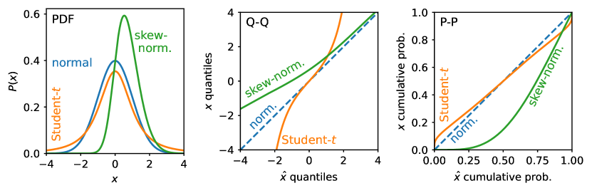
Figure 1: One-dimensional theoretical quantile–quantile (Q–Q) and probability–probability (P–P) plots comparing a normal distribution (blue) to two alternative distributions: a skew-normal (green), and a Student’s $t$-distribution (orange).

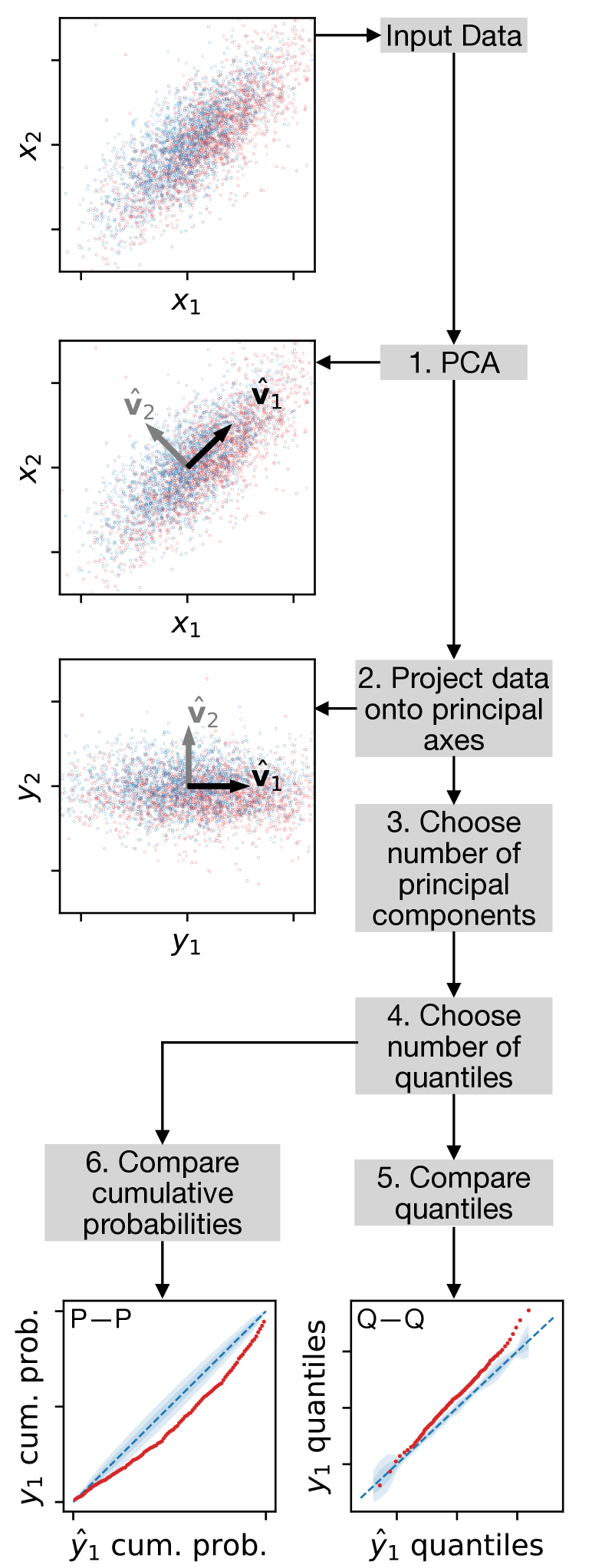
Figure 2: Schematic of the Q–Q and P–P plot-based validation scheme laid out in §2. The steps highlighted in the boxes of the flow chart correspond to the same steps in the mathematical description in Appendix A.

In this paper we present a widely-applicable method for comparing high dimensional samples that uses principal component analysis (PCA; Hotelling, 1933a, b, 1936) for dimensionality reduction, and Q–Q and P–P plots (Wilk & Gnanadesikan, 1968) for assessment. We also demonstrate a simple bootstrapping approach (following Maritz & Jarrett, 1978) for estimating uncertainties, thereby allowing for a quantitative assessment of the significance of deviations. Section 2 outlines our proposed methodology, with Section 3 containing several examples. We conclude in Section 4.

2 Method

The main ingredients of our proposed validation method are Q–Q and P–P plots. For two sets of samples, a Q–Q plot is constructed by calculating the coordinate values of a fixed number of quantiles for each set of samples, and then plotting the $q$th quantile of one sample against the $q$th quantile of the other. This creates a discrete curve which would show a one-to-one correspondence if the two distributions agreed perfectly. Q–Q plots give greater visual weight to discrepancies in the tails. A P–P plot plots the cumulative probability of one sample being below a certain value against the cumulative probability of the other sample being below the same value. This creates a plot bounded between zero and one, which should show a one-to-one correspondence in the case of perfect agreement. A simple one-dimensional example is shown in Figure 1. We augment the use of these plots in the case of high-dimensional models by using PCA in order to inspect and validate the model along a set of principal axes that captures most of the variability in the data.

The main steps of our method are shown in the flow-chart in Figure 2. In Appendix A we lay out the exact steps mathematically. Our method can be applied to any situation where one wishes to diagnose the difference between two distributions that are only represented by finite sets of samples.

We begin by selecting one set of samples – the data if validating model predictions – as our reference set, and the other as a test set. We then perform a PCA on the reference sample, and project both samples onto the principal axes of the reference. Next, we choose how many principal components to visualize (e.g. the number explaining 90% of the total variance of the data) and the number of quantiles to compute (see Hyndman & Fan, 1996 for a review of sample quantile estimation). In all of the examples we show in Section 3, we choose to plot percentiles (i.e. the coordinate values that divide the sorted dataset into 100 approximately equal pieces). This choice is made heuristically, as it gives good “resolution” of the distributions that are being compared without being excessively noisy in the tails. A Q–Q plot can then be produced by plotting the quantiles of the test sample against the quantiles of the reference sample (see lower right of Figure 2). A P–P plot is produced by comparing the cumulative probabilities for each sample at a range of coordinate values. This can done by counting the fraction of the test set that is smaller than each quantile of the reference set. The variances of the sample quantiles can be estimated via bootstrapping (Maritz & Jarrett, 1978; Efron, 1979), allowing the significance of deviations to be quantified.

3 Examples

We now present several demonstrations of the method outlined in Section 2. We begin with some two-dimensional toy models (§3.1 and §3.2) to give intuition for how different kinds of mismatch are manifested in Q–Q and P–P plots. We follow this with an applied example based on forward modeling galaxy photometric data (§3.3).

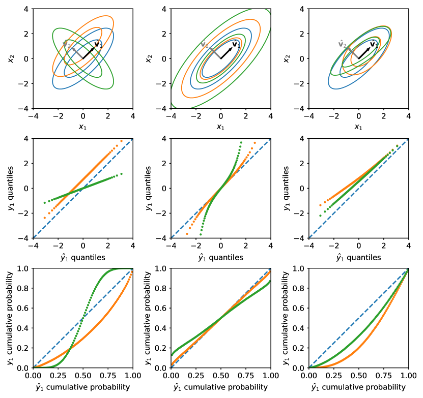
Figure 3: Two-dimensional illustration of quantile–quantile (Q–Q) and probability–probability (P–P) plots along a principal component axis. The upper row shows a variety of bivariate distributions in coordinate space. Our reference distribution (blue) is a multivariate normal in all three columns. In the first column, this is compared to a shifted (orange) and rotated (green) copy of the same distribution. In the second column the alternatives are a multivariate $t$-distribution with five d.o.f. (orange), and a multivariate Cauchy (green). In the third column, the alternate distributions are both bivariate skew-normals. The middle row shows Q–Q plots comparing the percentiles of the alternate distributions to the percentiles of the normal reference distribution. The comparison is made along the axis defined by the first principal component of the reference distribution (labelled $\hat{\bm{v}}_{1}$ in the upper panels). The bottom row shows the equivalent P–P plots.

3.1 Bivariate Normal Distribution

First, we will demonstrate the approach on some simple two dimensional examples. We use the bivariate normal distribution as a reference distribution, and compare this to several other multivariate distributions.

Figure 3 shows an assortment of bivariate distributions being compared to a bivariate normal distribution. The upper row of the figure shows the distributions in coordinate space, with the middle row showing Q–Q plots, and the bottom row showing P–P plots. We show the Q–Q and P–P plots along the first principal component axis of the reference distribution (indicated by the black arrow marked $\hat{\bm{v}}_{1}$ in the figure). For our reference distribution, we use a bivariate normal distribution with a zero mean vector, unit variance, and a correlation coefficient of 0.75 (shown in blue in all panels of Figure 3). The first principal eigenvector along which we will project all of the alternate distributions is $\hat{\bm{v}}_{1}=(1/\sqrt{2},1/\sqrt{2})^{\top}$.

In the left hand column of Figure 3 we compare our reference distribution to a shifted and a rotated copy of the same distribution. The shifted distribution (shown in orange) has the same covariance matrix as the reference distribution, but a mean vector of $(0,1)^{\top}$. This causes a translation away from the diagonal in the Q–Q plot, and a bowing beneath the diagonal in the P–P plot. The rotated distribution (shown in green) has a zero mean vector, unit variance, and a correlation coefficient of $-0.75$. Along the $\hat{\bm{v}}_{1}$ direction, this is under-dispersed relative to the reference distribution. In the Q–Q plot, under-/over-dispersion manifest as a straight line with a gradient of less/more than unity. In the P–P plot, under-dispersion shows as an S-shaped curve, with over-dispersion being a reflection of this about the diagonal.

In the middle column of Figure 3 we compare our reference distribution to a pair of heavier tailed distributions (i.e. a positive excess kurtosis compared to the normal distribution). In orange we show a multivariate $t$-distribution with 5 degrees of freedom, whilst in green we show a $t$-distribution with one degree of freedom (equivalent to a multivariate Cauchy distribution). For both of these distributions, we use a zero location vector, and scale matrix equal to the covariance of our normal reference distribution. In the Q–Q plots, mismatches of this kind can be seen as a divergence from the diagonal that increases towards the extremes. In the P–P plots, this causes a deviation from the diagonal. Compared to the case of higher variance, the P–P plots for the distributions with excess kurtosis show a much less pronounced turn back towards the diagonal.

In the right hand column of Figure 3 we compare our reference distribution to a pair of skewed/asymmetric distributions. These are both examples of the bivariate skew normal distribution (Azzalini & Dalla Valle, 1996; Azzalini & Capitanio, 1999). The orange distribution is skewed parallel to $\hat{\bm{v}}_{1}$, whilst the green has skewness in both directions. In the Q–Q plots, a skewness of this kind can be seen as a translation away from the diagonal, and a slight curvature. In the P–P plot, the skewness creates a bow shape that is less symmetric than the one created by a shift in mean (compare the oranges curves in the lower left and right panels of Figure 3.

3.2 Boomerang Distribution

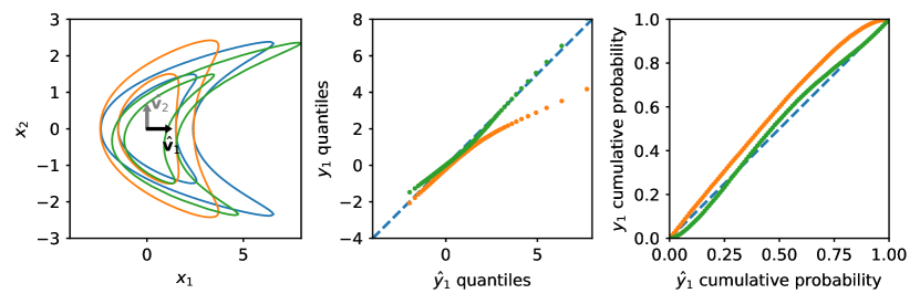
Figure 4: Same as Figure 3, but for a “boomerang” shaped distribution. We only compare along the first principal axis ($\hat{\bm{v}}_{1}$) here, as the marginals along the second axis are identical by construction.

In Figure 4, we show a more complex two dimensional example. Our reference distribution (blue), and alternative distributions (orange and green) are all “boomerang” transformations of a normal base density. For $\bm{z}=(z_{1},z_{2})^{\top}\sim N(\bm{0},\bm{\Sigma})$, we apply a transform given by

$$x_{2} =\theta_{2}z_{2}+\theta_{1},$$ (1)

$$x_{1} =\theta_{5}z_{1}+\theta_{3}\exp[\ln(|z_{2}|)\times\ln(1+e^{\theta_{4}})],$$ (2)

for a parameter vector $\bm{\theta}=(\theta_{1},\dots,\theta_{5})^{\top}$.

For the blue reference distribution and green alternate distribution in Figure 4, we set $\bm{\theta}=(0,1,1,2,1)^{\top}$. For the orange alternate distribution, we modify $\theta_{3}\to 0.5$. For blue and orange, we set the covariance matrix of the base distribution to the identity matrix, $\bm{\Sigma}=\bm{I}$. For green, we introduce set the off-diagonal term in $\bm{\Sigma}$ to 0.7 to introduce an asymmetry. The principal axes are parallel to the coordinate axes, and we only show the first principal component $\hat{\bm{v}}_{1}$ in the Q–Q and P–P plot since the marginals in the $\hat{\bm{v}}_{2}$ direction are all identical by construction. For the orange distribution, the behavior is close to the blue in the left tail, but diverges in the right tail due to the shorter “horns”. The divergence between the blue and green distributions varies in size and direction, with the divergences in the tails better highlighted by the Q–Q plot (middle panel), and the discrepancy in the central part showing more clearly in the P–P plot (right).

3.3 Forward-modeling Photometric Galaxy Catalogs

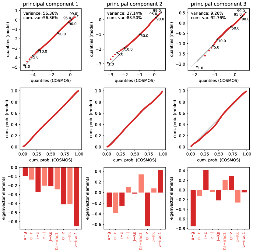
Figure 5: Quantile–quantile (QQ; top row) and probability–probability (PP; second row) plots comparing predictions from the pop-cosmos model (A24) to data from the COSMOS catalog (Weaver et al., 2022). Comparisons are shown for the first three principal axes of a set of nine broadband colors: $u-g$, $g-r$, $r-z$, $z-J$, $J-K_{s}$, $K_{s}-\texttt{irac1}$, $g-z$, $z-K_{s}$, and $z-\texttt{irac1}$. The contribution of each color to each principal eigenvector is shown in the bar chart in the bottom row of the figure. The most important principal component is in the left hand column, which explains around 56% of the total variance in the COSMOS data. Cumulatively, the three components shown explain 93% of the data’s variance.

In a companion paper by Alsing et al. (2024, hereafter A24), we use the methods developed by Alsing et al. (2020, 2023) and Leistedt et al. (2023) to construct a stellar population synthesis (SPS)-based forward model for the COSMOS photometric galaxy catalog (Weaver et al., 2022). We will hereafter refer to this model as pop-cosmos. The pop-cosmos model is trained to predict a distribution of magnitudes in 26 of the bands used in the COSMOS survey, based on a learned distribution of galaxy properties. This population distribution is represented by a score-based diffusion model (Song & Ermon, 2019, 2020; Song et al., 2020b, a) over 16 physical parameters that closely follow the parameterization used by Prospector-$\alpha$ (Leja et al., 2017, 2018, 2019b, 2019a). These physical parameters are translated into predictions of magnitudes in the 26 COSMOS bands by using an SPS emulator (Speculator; Alsing et al., 2020) and a flexible noise model based on a mixture density network (Bishop, 2006). Training of the pop-cosmos model is carried out by minimizing the Wasserstein distance (approximated using the Sinkhorn divergence; Cuturi, 2013; Feydy et al., 2019). In this section we use our proposed validation framework to compare predictions from the pop-cosmos model to the COSMOS data themselves.

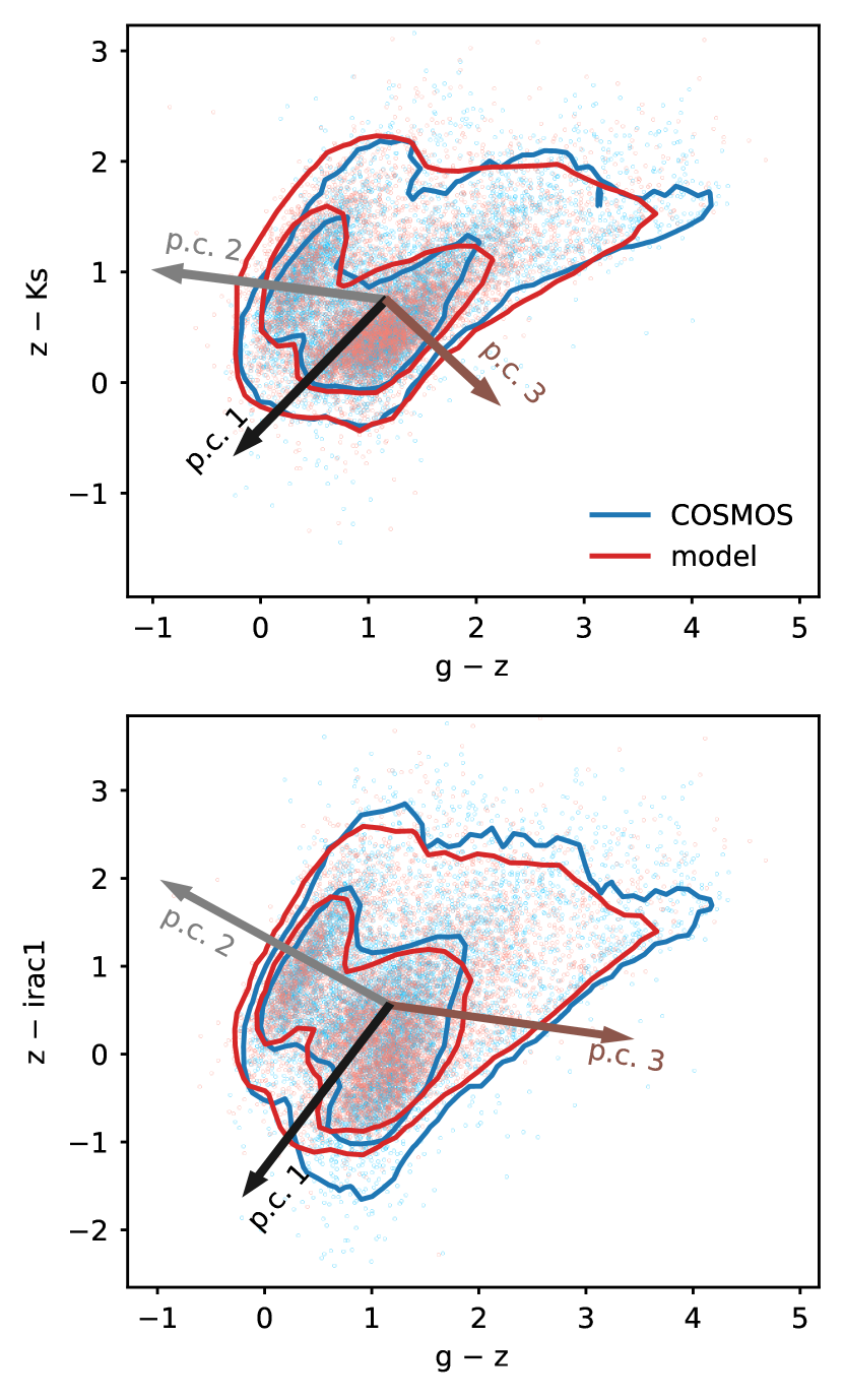
Figure 6: Color–color diagrams ($z-K_{s}$ and $z-\texttt{irac1}$ vs. $g-z$; c.f. figure 12 of Weaver et al., 2022). The first, second, and third principal eigenvectors of the COSMOS data are shown as black, grey, and brown arrows respectively. The light blue and light red points show the colors of 7,000 randomly selected galaxies from COSMOS ($\approx 5$% of the sample analysed in A24) and the pop-cosmos model. Contours are computed from the full sample, with the inner contours containing 68% of galaxies, and the outer contours containing 95%.

As detailed fully in A24, we apply an $r$-band magnitude cut of $r<25$ to both the data (leaving $\approx 140,000$ galaxies) and the model predictions and then compute an array of broadband colors for both sets of magnitudes. In particular, we consider the following nine colors: $u-g$, $g-r$, $r-z$, $z-J$, $J-K_{s}$, $K_{s}-\texttt{irac1}$, $g-z$, $z-K_{s}$, and $z-\texttt{irac1}$. The later three are highlighted in figure 12 of Weaver et al. (2022), whilst the remainder are highlighted in their figure 9 as being of particular importance to constraining galaxy properties via SED modeling.

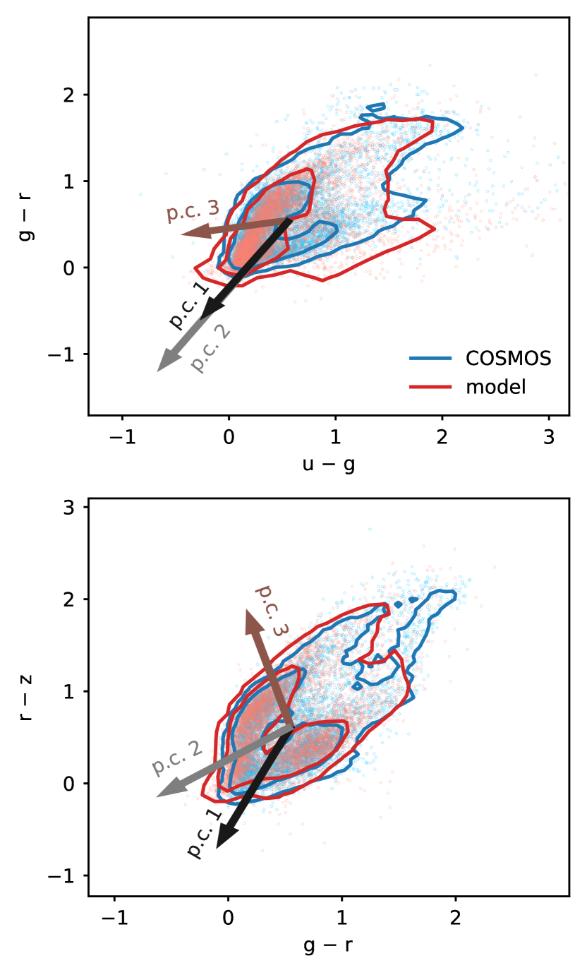
Figure 7: Same as Figure 6, but showing $g-r$ vs. $u-g$, and $r-z$ vs. $g-r$.

Figure 5 shows Q–Q and P–P plots for the first three principal components of our chosen list of colors. These three principal components cumulatively explain around 93% of the total variance in the COSMOS colors, with the first explaining around 56%. In this space, we compare the predicted color distributions from pop-cosmos (along the vertical axes in the top two rows) to the COSMOS data (along the horizontal axes of the top two rows). Due to the high number of objects, the variance of the sample quantiles is small, so the uncertainty band is very narrow. The bottom row of Figure 5 shows the contributions of the nine colors to each of the principal eigenvectors; this visualization serves to add interpretability to the findings.

The first principal component contains significant contributions from the full list of colors, weighted towards towards the three more widely-spaced colors ($g-z$, $z-K_{s}$, and $z-\texttt{irac1}$). The agreement seen between the pop-cosmos model and the data is visually very good along this principal axis, with slight deviations in the tails of the distribution.

The second principal component again contains substantial contributions from most of the colors apart from $z-J$, $J-K_{s}$, and $z-K_{s}$. Along this principal axis, we see deviation between the model predictions and the data below the 10th percentile – visible most clearly in the Q–Q plot in the upper centre of Figure 5. The agreement for the upper 90% of galaxies is good. The divergence seen on the edge suggests that the data are heavier tailed in the lower tail of this component. Figure 6 shows $z-K_{s}$ and $z-\texttt{irac1}$ vs. $g-z$ for COSMOS and pop-cosmos, with the second principal eigenvector of the COSMOS data shown as a grey arrow (p.c. 2). In both panels, it is noticeable that the COSMOS data has a slightly heavier lower tail in this direction (towards the right of the figure). Figure 7 shows that the $u-g$, $g-r$, and $r-z$ directions also contribute to this in the same way. Some of this disagreement could be due to difficulties with the COSMOS photometry in the $u$- and $g$-bands, which Weaver et al. (2022) find exhibit systematic differences between two different photometry catalogs (Classic, comparable to Laigle et al., 2016; and Farmer, based on Weaver et al., 2023). These systematics, and the relevance to the pop-cosmos model are discussed further by A24, who note that systematic offsets between the pop-cosmos model predictions and the COSMOS data are smaller than the offsets between Farmer and Classic.

The third principal axis is dominated by the $u-g$ color, and shows the strongest disagreement between model and data. Both the Q–Q and P–P plots show that the disagreement is more substantial below the median. Inspecting the upper panel of Figure 7, we can see that the model does not fully capture the structure of the data in the space of $g-r$ vs. $u-g$. In particular, the model predictions are much more concentrated into one side of the U-shape delineated by the inner blue contour (containing 68 per cent of the COSMOS galaxies). Some of this discrepancy may be explained by potential systematics in the data (discussed above), and the fact that the $u$- and $g$-bands tend to have a lower signal-to-noise and more very faint galaxies (c.f. figure 4 in A24).

4 Conclusions

We have presented a simple model checking and validation scheme that can be applied in any setting where two high-dimensional samples (e.g. model predictions and data) are to be compared. These situations are ubiquitous in astrophysics and cosmology – especially in the context of generative machine learning (ML). Our proposed approach is based on performing PCA on one of the samples and then comparing the two samples along the principal axes of the data. The comparison is made using quantile–quantile (Q–Q) and probability–probability (P–P) plots. We have demonstrated our methodology on a set of simple two-dimensional examples (Figure 3 and 4), to provide intuition for how different kinds of model mismatch are manifested in the Q–Q and P–P plots. We have then successfully applied our methodology to the validation of an ML-based generative model for galaxy photometry (pop-cosmos; A24).

We have demonstrated that the use of Q–Q and P–P plots in combination with PCA can be a useful tool to augment other more commonly used data space comparison techniques (e.g. comparing cumulative distribution functions, inspecting one- and two-dimensional marginal distributions). Although we have been motivated by validation of ML-based population models, the technique we have presented would be broadly applicable to any circumstance where two or more sets of samples from (potentially unknown) distribution are being compared.

A possible future development could be the adoption of QR-decomposition PCA (Sharma et al., 2013; de Souza et al., 2022) for improved scaling over covariance or singular-value decomposition approaches. Further investigation of the performance of our uncertainty quantification scheme (§A.3), including the consideration of alternative estimators (e.g. Bloch & Gastwirth, 1968) for the variance of sample quantiles (see discussion in Hall & Martin, 1988), may also be worthwhile.

Given the scale and fidelity of current (e.g. COSMOS, Scoville et al., 2007; Weaver et al., 2022; the Kilo Degree Survey, de Jong et al., 2013; Kuijken et al., 2019; the Dark Energy Survey, DES Collaboration, 2005; Abbott et al., 2018; Sevilla-Noarbe et al., 2021) and future (e.g. Euclid, Laureijs et al., 2011; the Vera C. Rubin Observatory’s Legacy Survey of Space and Time,Ivezić et al., 2019) datasets in cosmology, the use of generative ML and similar techniques will become the industry standard (for recent examples see Li et al., 2024; Moser et al., 2024; Alsing et al., 2024). The validation method we have presented here is well-suited to the challenge of interrogating the predictions of these models.

Author contributions. We outline the different contributions below using keywords based on the CRediT (Contribution Roles Taxonomy) system. ST: conceptualization, methodology, formal analysis, visualization, writing – original draft, writing – editing & review. HVP: conceptualization, methodology, validation, visualization, writing – editing & review, supervision, funding acquisition. DJM: conceptualization, methodology, validation, visualization, writing – editing & review. JA: data curation, validation, writing – editing & review. BL: methodology, writing – editing & review. SD: writing – editing & review.

Data availability. The data underlying this article will be shared on reasonable request to the corresponding author. An example notebook will be made available with the published version.

Acknowledgments. We thank George Efstathiou, Joel Leja, and Arthur Loureiro for useful discussions, and Davide Piras for providing a toy problem that was useful in the early stages of this work. ST, HVP, JA, and SD have been supported by funding from the European Research Council (ERC) under the European Union’s Horizon 2020 research and innovation programmes (grant agreement no. 101018897 CosmicExplorer). This work has been enabled by support from the research project grant ‘Understanding the Dynamic Universe’ funded by the Knut and Alice Wallenberg Foundation under Dnr KAW 2018.0067. HVP was additionally supported by the Göran Gustafsson Foundation for Research in Natural Sciences and Medicine. HVP and DJM acknowledge the hospitality of the Aspen Center for Physics, which is supported by National Science Foundation grant PHY-1607611. The participation of HVP and DJM at the Aspen Center for Physics was supported by the Simons Foundation. This research also utilized the Sunrise HPC facility supported by the Technical Division at the Department of Physics, Stockholm University. BL is supported by the Royal Society through a University Research Fellowship.

Appendix A Mathematical Description of the Testing Algorithm

A.1 Mathematical Outline

Here we outline an exact mathematical description of our proposed validation algorithm. Our inputs are two sets of samples of $D$-dimensional quantities (i.e. two $D$-dimensional point clouds), drawn from potentially unknown distributions. One of these sets of observations (of size $N$) is our reference distribution, which we will be comparing the other set (of size $M$) to. The $n$th observation in the reference set is a $D$-dimensional vector $\hat{\bm{x}}_{n}$, where hats are used because this is typically a sample of observed/measured values. The $m$th sample in the alternate set is a vector $\bm{x}_{m}$. The reference observations are combined into an $N\times D$ matrix $\hat{\bm{X}}$, whose $n$th row is $\hat{\bm{x}}_{n}^{\top}$. Similarly, we construct an $M\times D$ matrix $\bm{X}$, whose $m$th row is $\bm{x}_{m}^{\top}$.

With the inputs assembled, we proceed as follows:

1. Perform a PCA on the data:

   1. Compute the sample mean of the reference sample, $\hat{\bm{\mu}}=N^{-1}\sum_{n=1}^{N}\hat{\bm{x}}_{n}$;

   2. Compute the $D\times D$ covariance matrix of the reference sample, $\hat{\bm{C}}=(N-1)^{-1}\sum_{n=1}^{N}(\hat{\bm{x}}_{n}-\hat{\bm{\mu}})(\hat{\bm{x}}_{n}-\hat{\bm{\mu}})^{\top}$;

   3. Take an eigen-decomposition, $\hat{\bm{C}}=\hat{\bm{V}}\hat{\bm{\Lambda}}\hat{\bm{V}}^{-1}$, where $\hat{\bm{\Lambda}}=\operatorname{diag}(\hat{\bm{\lambda}})$, $\hat{\bm{\lambda}}=(\hat{\lambda}_{1},\dots,\hat{\lambda}_{D})^{\top}$ is a vector containing the $D$ eigenvalues of $\hat{\bm{C}}$ ordered from largest to smallest, and $\hat{\bm{V}}$ is a $D\times D$ matrix whose $d$th column $\hat{\bm{v}}_{d}$ contains the eigenvector corresponding to $\hat{\lambda}_{d}$.

2. Project both samples onto the principal axes defined by $\hat{\bm{V}}$, by computing $\hat{\bm{Y}}=\hat{\bm{X}}\hat{\bm{V}}$ and $\bm{Y}=\bm{X}\hat{\bm{V}}$. The $d$th column of $\hat{\bm{Y}}$, $\hat{\bm{y}}_{d}$, contains the projection of all observations onto the axis defined by $\hat{\bm{v}}_{d}$.

3. For a chosen fraction $f$ of the total variance, find the smallest $D_{\text{max}}$ satisfying $f\sum_{d=1}^{D}\hat{\lambda}_{d}\geq\sum_{d=1}^{D\text{max}}\hat{\lambda}_{d}$.

4. Choose $Q$, the number of quantiles to be computed. We define the $Q$ quantiles of a dataset as the coordinate values that partition the sorted dataset into $Q+1$ almost evenly sized pieces (§A.2).

5. For $d=1,\dots,D_{\text{max}}$, create a Q–Q plot:

   1. Extract the $d$th columns, $\hat{\bm{y}}_{d}$ and $\bm{y}_{d}$, from $\hat{\bm{Y}}$ and $\bm{Y}$, respectively;

   2. For $q=1,\dots,Q$, calculate the $q$th quantile of $\hat{\bm{y}}_{d}$ and $\bm{y}_{d}$, respectively $\hat{y}_{d}^{q}$ and $y_{d}^{q}$ (§A.2);

   3. Plot $\hat{y}_{d}^{q}$ vs. $y_{d}^{q}$ for all $q$;

   4. Estimate uncertainty via bootstrap (§A.3).

6. For $d=1,\dots,D_{\text{max}}$, create a P–P plot:

   1. Extract $\hat{\bm{y}}_{d}$ and $\bm{y}_{d}$ from $\hat{\bm{Y}}$ and $\bm{Y}$;

   2. For $q=1,\dots,Q$, calculate $\hat{y}_{d}^{q}$;

   3. Count $m_{q}$, the number of entries in $\bm{y}_{d}$ that are $<\hat{y}_{d}^{q}$;

   4. Plot $m_{q}/M$ vs. $q/(Q+1)$ for all q;

   5. Estimate uncertainty via bootstrap (§A.3).

7. (Optionally) Visualise each principal eigenvector $\bm{v}_{d}$ as a bar plot (see example in Figure 5).

A.2 Selection and Calculation of Quantiles

Here we elaborate further on the choice of $Q$ in step 4, and computation of quantiles in step 5b. We choose $Q=99$ – i.e. a partitioning of the data into 100. In our examples (including the real galaxy study in §3.3), we have $N,M\approx 100,000$ with $N\neq M$. It is a requirement that $Q\leq\min(N,M)$. For $N=M$, one can set $Q=N$ and trivially produce a Q–Q plot by plotting the sorted entries of $\bm{y}$ against the sorted entries of $\hat{\bm{y}}$. However, it is preferable to set $Q\ll\min(N,M)$. This makes generalisation to $N\neq M$ more straightforward. It also avoids excessive variance in the estimates of $\hat{y}^{q}$ and $y^{q}$ as $q\to 1$ and $q\to Q$.

The algorithm for computing $\hat{y}^{q}$ and $y^{q}$ is also a choice that must be made. For a comprehensive review of quantile estimation, see Hyndman & Fan (1996). For $\hat{\bm{y}}$ of length $N$, we can compute a pseudo-index $i=Nq/(Q+1)$ for the $q$th quantile $\hat{y}^{q}$. If $N/(Q+1)$ is an integer (i.e. if an exact partitioning of the dataset is possible), $\hat{y}^{q}$ will be the $i$th largest entry in $\hat{\bm{y}}$. Otherwise, an approximation must be used. The simplest and most intuitive method is a “nearest rank” approach where one calculates $g=i-\lfloor i\rfloor$ and takes the $\lceil i\rceil$th largest entry of $\hat{\bm{y}}$ if $g\geq 0.5$, or the the $\lfloor i\rfloor$th largest entry if $g<0.5$. This produces a discontinuous estimator for $\hat{y}^{q}$. The default option in the NumPy library (Harris et al., 2020), which we use throughout this work, is a piecewise linear interpolation scheme proposed by Gumbel (1939) and presented as definition 7 in Hyndman & Fan (1996). This produces an estimate of $\hat{y}^{q}$ that is continuous as a function of $q/(Q+1)$.

A.3 Uncertainty Quantification

Here we outline algorithms based on bootstrapping (Efron, 1979) that can be used to quantify uncertainty on Q–Q and P–P plots (steps 5d and 6e in §A). A bootstrap estimator for the variance of sample quantiles was first introduced by Maritz & Jarrett (1978), with its properties proven by Hall & Martin (1988). For a data vector $\hat{\bm{y}}$ of length $N$, we can estimate the variance of the $q$th quantile $\hat{y}^{q}$ as follows:

1. Select a number ($B$) of bootstrapped realisations to sample.

2. For $b=1,\dots,B$:

   1. construct a new vector $\hat{\bm{\gamma}}_{b}$ of length $N$ by sampling with replacement from $\hat{\bm{y}}$;

   2. estimate the $q$th quantile $\hat{\gamma}_{b}^{q}$ of $\hat{\bm{\gamma}}_{b}$ using the usual procedure (§A.2).

3. Estimate the variance $\hat{\sigma}_{q}^{2}=B^{-1}\sum_{b=1}^{B}(\hat{\gamma}_{b}^{q}-\hat{y}^{q})^{2}$.

This allows us to show a confidence region on the diagonal of a Q–Q plot, thereby quantifying the significance of deviations. Similarly, for a P–P plot, we can estimate the variance of the cumulative probability estimates:

1. Select a number ($B$) of bootstrapped realisations to sample.

2. For $b=1,\dots,B$:

   1. construct a new vector $\hat{\bm{\gamma}}_{b}$ of length $N$ by sampling with replacement from $\hat{\bm{y}}$;

   2. count $n_{b}^{q}$, the number of entries in $\hat{\bm{\gamma}}_{b}$ $<\hat{y}^{q}$;

   3. compute $p_{b}^{q}=n_{b}^{q}/N$.

3. Find the variance $\hat{\sigma}_{q}^{2}=B^{-1}\sum_{b=1}^{B}[p_{b}^{q}-q/(Q+1)]^{2}$.

In this way, it is also possible to show a confidence region on a P–P plot.

References

- Abbott et al. (2018) Abbott, T. M. C., Abdalla, F. B., Allam, S., et al. 2018, ApJS, 239, 18, doi: 10.3847/1538-4365/aae9f0
- Abbott et al. (2019) Abbott, T. M. C., Abdalla, F. B., Alarcon, A., et al. 2019, Phys. Rev. D, 100, 023541, doi: 10.1103/PhysRevD.100.023541
- Alsing et al. (2023) Alsing, J., Peiris, H., Mortlock, D., Leja, J., & Leistedt, B. 2023, ApJS, 264, 29, doi: 10.3847/1538-4365/ac9583
- Alsing et al. (2024) Alsing, J., Thorp, S., Deger, S., et al. 2024, arXiv e-prints, arXiv:2402.00935, doi: 10.48550/arXiv.2402.00935
- Alsing et al. (2020) Alsing, J., Peiris, H., Leja, J., et al. 2020, ApJS, 249, 5, doi: 10.3847/1538-4365/ab917f
- Azzalini & Capitanio (1999) Azzalini, A., & Capitanio, A. 1999, J. R. Statistical Soc. Series B, 61, 579, doi: 10.1111/1467-9868.00194
- Azzalini & Dalla Valle (1996) Azzalini, A., & Dalla Valle, A. 1996, Biometrika, 83, 715, doi: 10.1093/biomet/83.4.715
- Bishop (2006) Bishop, C. M. 2006, Pattern Recognition and Machine Learning (Springer)
- Bloch & Gastwirth (1968) Bloch, D. A., & Gastwirth, J. L. 1968, Ann. Math. Statistics, 39, 1083 , doi: 10.1214/aoms/1177698342
- Buchner & Boorman (2023) Buchner, J., & Boorman, P. 2023, arXiv e-prints, arXiv:2309.05705, doi: 10.48550/arXiv.2309.05705
- Challener et al. (2023) Challener, R. C., Welbanks, L., & McGill, P. 2023, arXiv e-prints, arXiv:2310.03733, doi: 10.48550/arXiv.2310.03733
- Chevallard & Charlot (2016) Chevallard, J., & Charlot, S. 2016, MNRAS, 462, 1415, doi: 10.1093/mnras/stw1756
- Cramér (1928) Cramér, H. 1928, Scandinavian Actuarial J., 1928, 13, doi: 10.1080/03461238.1928.10416862
- Cuturi (2013) Cuturi, M. 2013, in Advances in Neural Information Processing Systems, ed. C. Burges, L. Bottou, M. Welling, Z. Ghahramani, & K. Weinberger, Vol. 26 (Curran Associates, Inc.). https://arxiv.org/abs/1306.0895
- de Jong et al. (2013) de Jong, J. T. A., Kuijken, K., Applegate, D., et al. 2013, The Messenger, 154, 44
- de Souza et al. (2022) de Souza, R. S., Quanfeng, X., Shen, S., Peng, C., & Mu, Z. 2022, Astron. & Comput., 41, 100633, doi: 10.1016/j.ascom.2022.100633
- DES Collaboration (2005) DES Collaboration. 2005, arXiv e-prints, astro-ph/0510346, doi: 10.48550/arXiv.astro-ph/0510346
- Eadie et al. (2023) Eadie, G. M., Speagle, J. S., Cisewski-Kehe, J., et al. 2023, arXiv e-prints, arXiv:2302.04703, doi: 10.48550/arXiv.2302.04703
- Efron (1979) Efron, B. 1979, Ann. Statistics, 7, 1 , doi: 10.1214/aos/1176344552
- Feeney et al. (2019) Feeney, S. M., Peiris, H. V., Williamson, A. R., et al. 2019, Phys. Rev. Lett., 122, 061105, doi: 10.1103/PhysRevLett.122.061105
- Feydy et al. (2019) Feydy, J., Séjourné, T., Vialard, F.-X., et al. 2019, in Proc. Machine Learning Res., Vol. 89, Proceedings of the Twenty-Second International Conference on Artificial Intelligence and Statistics, ed. K. Chaudhuri & M. Sugiyama (PMLR), 2681–2690. https://arxiv.org/abs/1810.08278
- Gelman et al. (1996) Gelman, A., Meng, X.-L., & Stern, H. 1996, Statistica Sinica, 6, 733. http://www.jstor.org/stable/24306036
- Gumbel (1939) Gumbel, E. J. 1939, Comptes Rendus Acad. Sci., 209, 645
- Hall & Martin (1988) Hall, P., & Martin, M. 1988, Probability Theor. & Related Fields, 80, 261, doi: 10.1007/BF00356105
- Harris et al. (2020) Harris, C. R., Millman, K. J., van der Walt, S. J., et al. 2020, Nature, 585, 357, doi: 10.1038/s41586-020-2649-2
- Hotelling (1933a) Hotelling, H. 1933a, J. Educational Psychcology, 24, 417, doi: 10.1037/h0071325
- Hotelling (1933b) —. 1933b, J. Educational Psychcology, 24, 498, doi: 10.1037/h0070888
- Hotelling (1936) —. 1936, Biometrika, 28, 321, doi: 10.1093/biomet/28.3-4.321
- Hunter (2007) Hunter, J. D. 2007, Comput. Sci. Eng., 9, 90, doi: 10.1109/MCSE.2007.55
- Huppenkothen et al. (2013) Huppenkothen, D., Watts, A. L., Uttley, P., et al. 2013, ApJ, 768, 87, doi: 10.1088/0004-637X/768/1/87
- Hyndman & Fan (1996) Hyndman, R. J., & Fan, Y. 1996, American Statistician, 50, 361, doi: 10.2307/2684934
- Ivezić et al. (2019) Ivezić, Ž., Kahn, S. M., Tyson, J. A., et al. 2019, ApJ, 873, 111, doi: 10.3847/1538-4357/ab042c
- Kolmogorov (1933) Kolmogorov, A. 1933, G. Istituto Ital. Attuari, 4, 83
- Kuijken et al. (2019) Kuijken, K., Heymans, C., Dvornik, A., et al. 2019, A&A, 625, A2, doi: 10.1051/0004-6361/201834918
- Laigle et al. (2016) Laigle, C., McCracken, H. J., Ilbert, O., et al. 2016, ApJS, 224, 24, doi: 10.3847/0067-0049/224/2/24
- Laureijs et al. (2011) Laureijs, R., Amiaux, J., Arduini, S., et al. 2011, arXiv e-prints, arXiv:1110.3193, doi: 10.48550/arXiv.1110.3193
- Leistedt et al. (2023) Leistedt, B., Alsing, J., Peiris, H., Mortlock, D., & Leja, J. 2023, ApJS, 264, 23, doi: 10.3847/1538-4365/ac9d99
- Leja et al. (2019a) Leja, J., Carnall, A. C., Johnson, B. D., Conroy, C., & Speagle, J. S. 2019a, ApJ, 876, 3, doi: 10.3847/1538-4357/ab133c
- Leja et al. (2018) Leja, J., Johnson, B. D., Conroy, C., & van Dokkum, P. 2018, ApJ, 854, 62, doi: 10.3847/1538-4357/aaa8db
- Leja et al. (2017) Leja, J., Johnson, B. D., Conroy, C., van Dokkum, P. G., & Byler, N. 2017, ApJ, 837, 170, doi: 10.3847/1538-4357/aa5ffe
- Leja et al. (2019b) Leja, J., Johnson, B. D., Conroy, C., et al. 2019b, ApJ, 877, 140, doi: 10.3847/1538-4357/ab1d5a
- Li et al. (2024) Li, J., Melchior, P., Hahn, C., & Huang, S. 2024, AJ, 167, 16, doi: 10.3847/1538-3881/ad0be4
- Maritz & Jarrett (1978) Maritz, J. S., & Jarrett, R. G. 1978, J. American Statistical Association, 73, 194, doi: 10.2307/2286545
- McGill et al. (2023) McGill, P., Anderson, J., Casertano, S., et al. 2023, MNRAS, 520, 259, doi: 10.1093/mnras/stac3532
- Meng (1994) Meng, X.-L. 1994, Ann. Statistics, 22, 1142 , doi: 10.1214/aos/1176325622
- Moser et al. (2024) Moser, B., Kacprzak, T., Fischbacher, S., et al. 2024, arXiv e-prints, arXiv:2401.06846, doi: 10.48550/arXiv.2401.06846
- Nixon et al. (2023) Nixon, M. C., Welbanks, L., McGill, P., & Kempton, E. M. R. 2023, arXiv e-prints, arXiv:2310.03713, doi: 10.48550/arXiv.2310.03713
- Park et al. (2008) Park, T., van Dyk, D. A., & Siemiginowska, A. 2008, ApJ, 688, 807, doi: 10.1086/591631
- Paszke et al. (2019) Paszke, A., Gross, S., Massa, F., et al. 2019, in Advances in Neural Information Processing Systems, ed. H. Wallach, H. Larochelle, A. Beygelzimer, F. d'Alché-Buc, E. Fox, & R. Garnett, Vol. 32 (Curran Associates, Inc.). https://arxiv.org/abs/1912.01703
- Protassov et al. (2002) Protassov, R., van Dyk, D. A., Connors, A., Kashyap, V. L., & Siemiginowska, A. 2002, ApJ, 571, 545, doi: 10.1086/339856
- Rogers & Peiris (2021) Rogers, K. K., & Peiris, H. V. 2021, Phys. Rev. D, 103, 043526, doi: 10.1103/PhysRevD.103.043526
- Rubin (1984) Rubin, D. B. 1984, Ann. Statistics, 12, 1151 , doi: 10.1214/aos/1176346785
- Scoville et al. (2007) Scoville, N., Aussel, H., Brusa, M., et al. 2007, ApJS, 172, 1, doi: 10.1086/516585
- Sevilla-Noarbe et al. (2021) Sevilla-Noarbe, I., Bechtol, K., Carrasco Kind, M., et al. 2021, ApJS, 254, 24, doi: 10.3847/1538-4365/abeb66
- Sharma et al. (2013) Sharma, A., Paliwal, K., Imoto, S., & Miyano, S. 2013, Int. J. Machine Learning & Cybernetics, 4, 679, doi: 10.1007/s13042-012-0131-7
- Smirnov (1948) Smirnov, N. 1948, Ann. Math. Statistics, 19, 279 , doi: 10.1214/aoms/1177730256
- Song et al. (2020a) Song, J., Meng, C., & Ermon, S. 2020a, arXiv e-prints, arXiv:2010.02502, doi: 10.48550/arXiv.2010.02502
- Song & Ermon (2019) Song, Y., & Ermon, S. 2019, in Advances in Neural Information Processing Systems, ed. H. Wallach, H. Larochelle, A. Beygelzimer, F. d'Alché-Buc, E. Fox, & R. Garnett, Vol. 32 (Curran Associates, Inc.). https://arxiv.org/abs/1907.05600
- Song & Ermon (2020) Song, Y., & Ermon, S. 2020, in Advances in Neural Information Processing Systems, ed. H. Larochelle, M. Ranzato, R. Hadsell, M. Balcan, & H. Lin, Vol. 33 (Curran Associates, Inc.), 12438–12448. https://arxiv.org/abs/2006.09011
- Song et al. (2020b) Song, Y., Sohl-Dickstein, J., Kingma, D. P., et al. 2020b, arXiv e-prints, arXiv:2011.13456, doi: 10.48550/arXiv.2011.13456
- Stein et al. (2015) Stein, N. M., van Dyk, D. A., Kashyap, V. L., & Siemiginowska, A. 2015, ApJ, 813, 66, doi: 10.1088/0004-637X/813/1/66
- Vehtari et al. (2017) Vehtari, A., Gelman, A., & Gabry, J. 2017, Statistics & Comput., 27, 1413, doi: 10.1007/s11222-016-9696-4
- Virtanen et al. (2020) Virtanen, P., Gommers, R., Oliphant, T. E., et al. 2020, Nature Methods, 17, 261, doi: 10.1038/s41592-019-0686-2
- von Mises (1928) von Mises, R. 1928, Wahrscheinlichkeit Statistik und Wahrheit (Springer)
- Weaver et al. (2022) Weaver, J. R., Kauffmann, O. B., Ilbert, O., et al. 2022, ApJS, 258, 11, doi: 10.3847/1538-4365/ac3078
- Weaver et al. (2023) Weaver, J. R., Zalesky, L., Kokorev, V., et al. 2023, ApJS, 269, 20, doi: 10.3847/1538-4365/acf850
- Welbanks et al. (2023) Welbanks, L., McGill, P., Line, M., & Madhusudhan, N. 2023, AJ, 165, 112, doi: 10.3847/1538-3881/acab67
- Wilk & Gnanadesikan (1968) Wilk, M. B., & Gnanadesikan, R. 1968, Biometrika, 55, 1, doi: 10.1093/biomet/55.1.1