The Fragile Nature of Road Transportation Systems

Abstract

Major cities worldwide experience problems with the performance of their road transportation systems, and the continuous increase in traffic demand presents a substantial challenge to the optimal operation of urban road networks and the efficiency of traffic control strategies. Although robust and resilient transportation systems have been extensively researched over the past decades, their performance under an ever-growing traffic demand can still be questionable. The operation of transportation systems is widely believed to display fragile property, i.e., the loss in performance increases exponentially with the linearly increasing magnitude of disruptions, which undermines their continuous operation. Nowadays, the risk engineering community is embracing the novel concept of antifragility, which enables systems to learn from historical disruptions and exhibit improved performance as disruption levels reach unprecedented magnitudes. In this study, we demonstrate the fragile nature of road transportation systems when faced with demand or supply disruptions. First, we conducted a rigorous mathematical analysis to establish the fragile nature of the systems theoretically. Subsequently, by taking into account real-world stochasticity, we implemented a numerical simulation with realistic network data to bridge the gap between the theoretical proof and the real-world operations, to reflect the potential impact of uncertainty on the fragile property of the systems. This work aims to demonstrate the fragility of road transportation systems and help researchers better comprehend the necessity to explicitly consider antifragile design for future traffic control strategies, coping with the constantly growing traffic demand and subsequent traffic accidents.

[a]organization=Institute for Transport Planning and Systems, ETH Zurich, city=Zurich, postcode=8093, country=Switzerland [b]organization=Computer Science Department and Center for Artificial Intelligence, Technische Hochschule Nürnberg, city=Nürnberg, postcode=90489, country=Germany [c]organization=Intelligent Cloud Technologies Lab, Huawei Munich Research Center, city=Munich, postcode=80992, country=Germany

1 Introduction

As reported by both the U.S. Department of Transportation (2019) and Federal Statistical Office of Switzerland (2020), motorized road traffic before the pandemic has experienced an approximate 50% growth over the past few decades. Researchers have also found that the continuous growth in traffic volume has consequently contributed to a rise in disruptive events, such as severe congestion and more frequent accidents (Dickerson et al., 2000; Chang and Xiang, 2003). With evidence confirming the recovery of individual motorized traffic from the pandemic (Büchel et al., 2022; Marra et al., 2022; Ciuffini et al., 2023), it is expected that this upward trend will continue in the coming decades (Zhang and Zhang, 2021).

Meanwhile, there is a common understanding that road transportation networks can exhibit fragile properties. Fragility signifies a system’s susceptibility to exponentially escalating performance deterioration as disruptions increase in magnitude. One prominent example of such fragile characteristics is the BPR function (U.S. Bureau of Public Roads, 1964), which distinctly illustrates with empirical data at the link level that travel time grows exponentially with traffic flow, leading to an infinite temporal cost when the traffic influx is at the maximal density of the network. Moreover, not limited to urban road networks, many other types of transportation systems can also display similar fragile responses to increasing disruption levels, such as in railway (Gibson et al., 2002; Saidi et al., 2023) and aviation systems (U.S. Congress, Office of Technology Assessment, 1984).

Researchers have devoted extensive efforts to the assessment and design of robust and resilient transportation systems of all kinds, such as in railway systems (Corman et al., 2014; Larsen et al., 2014), public transportation operation (Cats, 2016; Fuchs and Corman, 2019), aviation (Isaacson et al., ), and road networks (Ampountolas et al., 2017; Yang et al., 2019; Leclercq et al., 2021). However, when accounting for the ever-growing traffic volume in urban road networks and the exponentially escalating adversarial consequences, it is natural for us to wonder whether the current level of robustness and resilience can still guarantee the performance of road networks considering a long-term time horizon. Hence, we introduce the cutting-edge concept of antifragility to explain the phenomenon that roadside performance deteriorates exponentially with linearly growing disruptions. Previous studies discussing the fragile response, such as the BPR function, have primarily relied on empirical data and intuitive reasoning rather than rigorous mathematical proof. This paper, on the other hand, serves as a proof of concept, aiming to establish the fragile nature of road transportation systems through mathematical analysis. Additionally, as stochasticity prevails in transportation systems in the real world, we also designed a numerical simulation considering real-world stochasticity, to study to what extent such realistic uncertainties can influence the fragile characteristics of transportation systems. The overarching objective of this paper is to provide insights to transportation researchers for the future design of transportation systems and control strategies to be not only robust and resilient but also antifragile.

The remainder of this paper is structured as follows. Section 2 introduces antifragility and reviews specific traffic-related mathematical models. Section 3 formulates the mathematical definition of (anti-)fragility and its applications. Then we conduct the mathematical proof in Section 4, whereas Section 5 presents the numerical simulation with real-world network and stochasticity. With Section 6, we conclude the fragile nature of road transportation systems and its implications for future studies.

2 Relevant Literature

Various terminologies have been proposed to evaluate the performance of road transportation systems, including their control strategies, and two commonly used terms to characterize the extent of performance variations under stress are robustness (Duan and Lu, 2014; Shang et al., 2022) and resilience (Mattsson and Jenelius, 2015; Calvert and Snelder, 2018). However, the definitions of robustness and resilience can vary under different contexts, even within the transportation domain itself, and are sometimes used interchangeably due to the different backgrounds and points of view of the authors (Tang et al., 2020; Corman et al., 2018). In this study, we adopt the definition proposed in Zhou et al. (2019), wherein robustness involves evaluating a system’s ability to maintain its initial state and withstand performance degradation when confronted with uncertainties and disturbances. On the other side, resilience emphasizes a system’s capability and promptness in recovering from major disruptions and returning to its original state. In brief, robustness relates to resistance, whereas resilience is about recovery.

Nevertheless, these two terms can overlook the consideration of a longer timespan and the potential escalation of disruptions, which is particularly relevant in transportation as the traffic demand grows continuously and consequently so as the occurrences of accidents. Thus, there is the necessity to introduce a new term to address this gap. The novel concept of antifragility was initially proposed in Taleb (2012) and mathematically elaborated in Taleb and Douady (2013); Taleb and West (2023), and it serves as a general concept aimed at transforming people’s understanding and perception of risk. By embracing current risks, we can potentially leverage and adapt to future risks of greater magnitudes. When employed in systems and control, (anti-)fragility can be conceptualized as a nonlinear relationship between the performance and the magnitude of disruptions. If the performance is compromised due to unexpected disruptions, the relationship between the loss in performance and the disruptions would be convex for a fragile system, while being concave for an antifragile system. Ever since being proposed, antifragility has gained popularity in the risk engineering community across multiple disciplines, such as economy (Manso et al., 2020), biology (Kim et al., 2020), medicine (Axenie et al., 2022), energy (Coppitters and Contino, 2023), robotics (Axenie and Saveriano, 2023), and lately in transportation (Sun et al., 2024). It should also be highlighted that although systems can be fragile by nature, proper intervention and control strategies can enhance their antifragility against increasing disruptions (Axenie et al., 2023).

In transportation, by unveiling the convex relationship between travel time and traffic flow with empirical data, the BPR function (U.S. Bureau of Public Roads, 1964), as shown in Eq. 1 has given an intuitive example showing the fragility of the transportation systems on a link level. Together with its variations (Dowling and Skabardonis, 1993; Skabardonis and Dowling, 1997), the BPR function has been extensively applied in the estimation of the link (route) travel time (Lo et al., 2006; Ng and Waller, 2010; Wang et al., 2014). However, to uphold the statement that road transportation systems are fragile in general, an empirical function like BPR alone is not sufficient without rigid mathematical proof. It is also desired to show the fragility more broadly, i.e., not only on the link level but also on the macroscopic level, as well as for different types of disruptions.

$$T =T_{ff}\left(1+\alpha\left(\frac{q}{q_{\rm max}}\right)^{\beta}\right)$$ (1)

The assessment of traffic performance can be conducted at either the microscopic or macroscopic level, sometimes also mesoscopically (Zehe et al., 2015). However, due to the non-identical traffic characteristics across different levels, researchers have formulated diverse models to offer a more precise description of traffic dynamics on different levels. While some models are generated numerically from data, others are derived through analytical methods (Mariotte et al., 2017).

The earliest study on traffic performance was carried out and described in Greenshields et al. (1934) on a section of a highway and yielded the first Fundamental Diagram (FD), as shown in Fig. 1(a), which exhibits the relationship between traffic flow, denoted as $q$, and density, denoted as $k$, in the shape of a second-degree polynomial. Later, other researchers also developed FDs in various forms, with one of the most commonly applied FDs being proposed in Daganzo (1994), as shown in Fig. 1(b), which is characterized by two linear functions. While the Greenshields FD is entirely generated through fitting the polynomial coefficients with on-site data, the Daganzo FD, on the other hand, is derived analytically by treating the traffic flow hydrodynamically and incorporates variables with physical meanings, i.e., the free-flow speed, back-propagation speed, and critical density, denoted as $v_{f}$, $w$, and $k_{c}$, respectively.

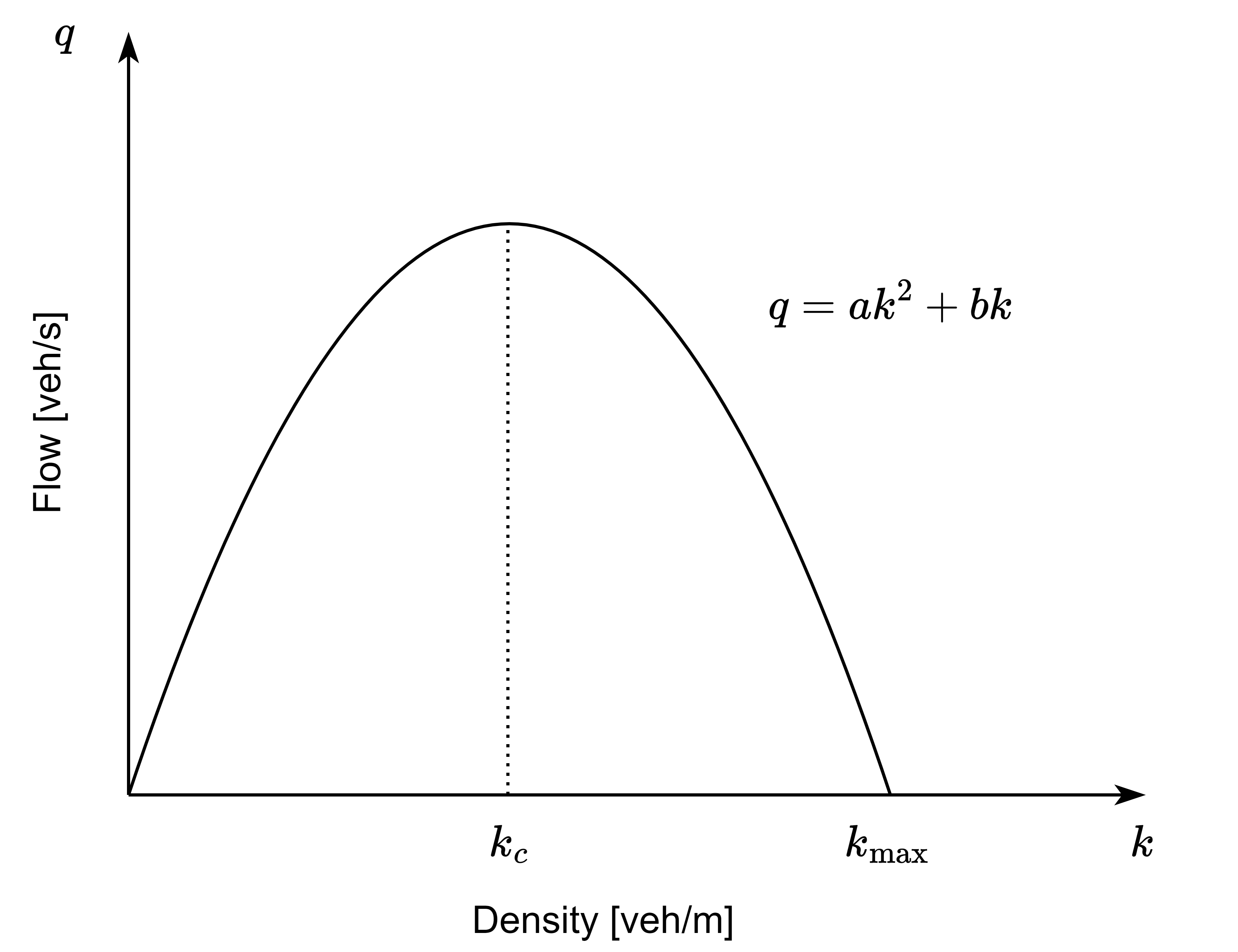
(a) Greenshields 2nd-degree polynomial FD (1934)

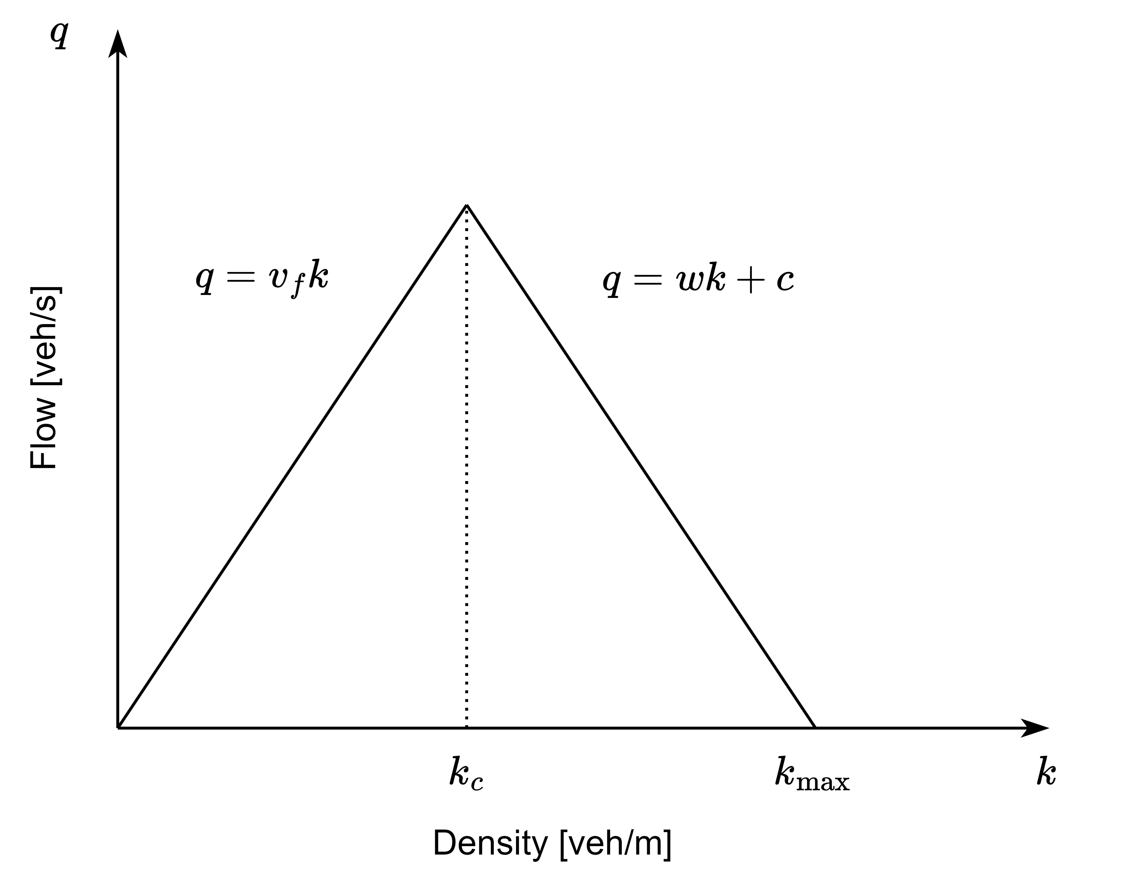
(b) Daganzo two-regime linear FD (1994)

Figure 1: Mathematical models of FDs

On the network level, with the assumption of a homogeneous region, a Macroscopic Fundamental Diagram (MFD) can be produced by aggregating data points gathered from representative links within this network. Similar to FDs, MFDs can be approximated through different models, and the most widely applied approaches include polynomials and multi-regime linear functions. MFDs can be fit numerically from field measurements as a cubic polynomial, as in Haddad and Shraiber (2014); Sirmatel and Geroliminis (2018) and illustrated in Fig. 2(a), and therefore, it’s commonly seen in research works simulating traffic control on a macroscopic level with a given MFD. On the other hand, based on the framework of variation theory (Daganzo, 2005), Daganzo and Geroliminis (2008) is the first study to analytically generate an MFD, and is often referred to as the Method of Cuts (MoC). Instead of installing loop detectors under the pavement and gathering massive traffic flow data, MoC can be applied to derive an MFD directly from roadside variables with physical meanings, such as free flow speed, traffic signal cycle, lane length, etc. An example of multi-regime linear functions MFD from MoC is shown in Fig. 2(b). Leclercq and Geroliminis (2013) modified the original MoC to accommodate topology and signal timing heterogeneity within the network. Although theoretically an infinite number of cuts can be generated to approximate the MFD, only the practical cuts, the solid lines as shown in Fig. 2(b), are used for simplicity reasons. Although some other analytical methods have also been proposed to produce an MFD, such as through stochastic approximation (Laval and Castrillón, 2015), Tilg et al. (2020) has demonstrated that MoC yields a more accurate upper bound for the MFD. Lately, researchers have also explored the potential utilization of MFD in railway (Corman et al., 2019) and aviation operations (Safadi et al., 2023), which yields some positive possibilities of extending the MFD into other modes.

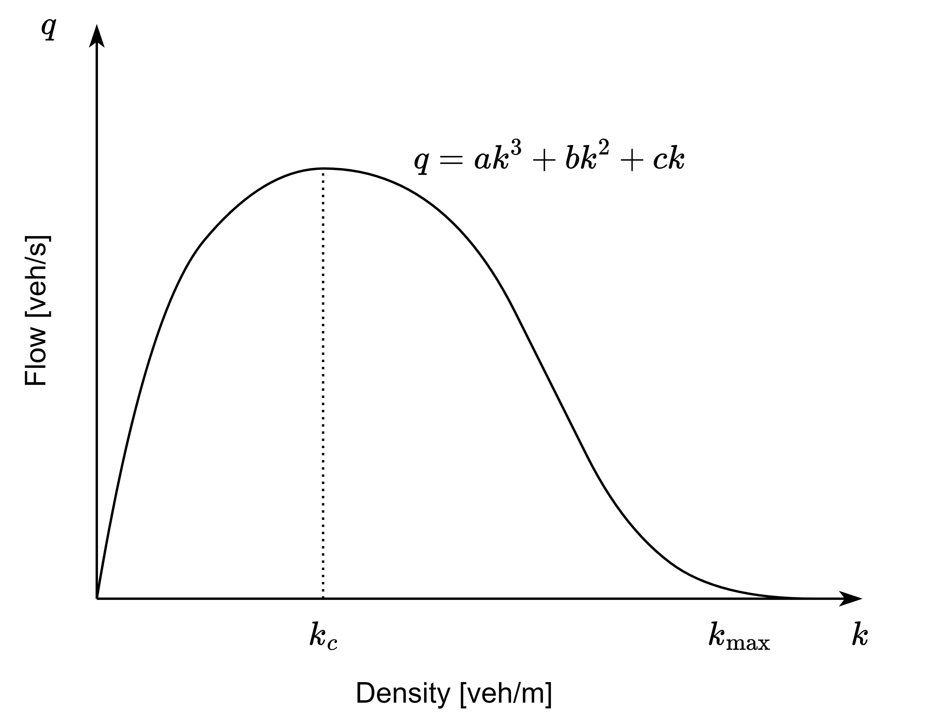
(a) Geroliminis 3rd-degree polynomial MFD (2013)

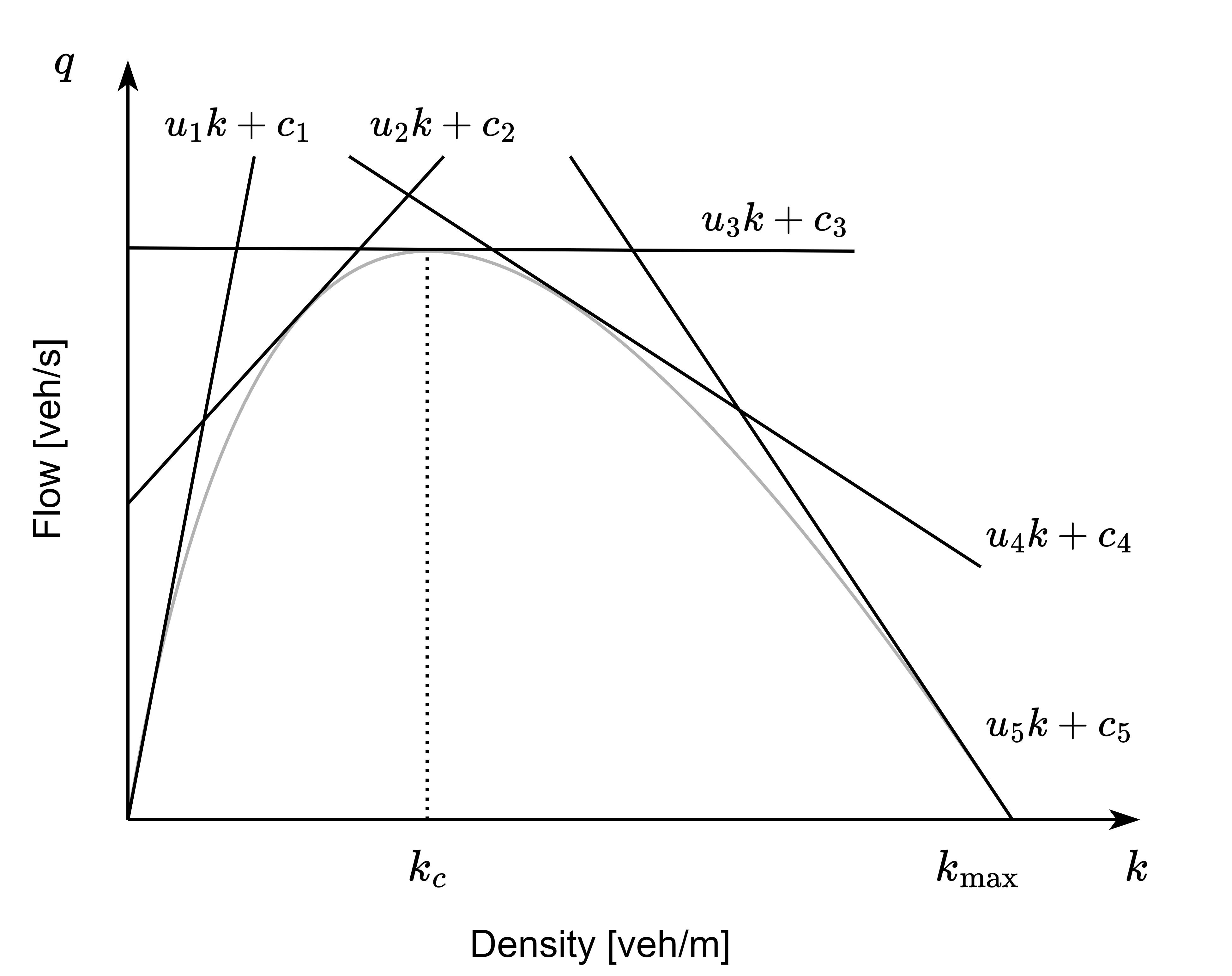
(b) Daganzo multi-regime linear MFD (2008)

Figure 2: Mathematical models of MFDs

As also acknowledged in these works, some variables, particularly the parameters related to signalization, can be hard to acquire in the real world with actuated signals. Therefore, simplified MFDs are also widely adopted when solving more applicational problems in the real world. Daganzo et al. (2018) approximated a simplified MoC-based MFD using only three cuts from one of each stationary, forward, and backward observer, and formed the uMFD. Another shortcoming of the numerical-based MFD is that, since the data points near the maximal density are scarce overall, the approximated MFD can lose its fidelity near the maximal density. For example, the third-degree polynomial in Geroliminis et al. (2013) has only one real root, indicating the speed is above zero despite the fact that the network has already reached a gridlock, which cannot be realistic. As claimed in Daganzo and Geroliminis (2008), since MFDs should be concave, the flow and speed are both zero by definition at maximal density.

3 Problem formulation

As explained in Section 2, an (anti-)fragile response of a system can be characterized through a nonlinear relationship between the performance loss and the magnitude of the disruption, as shown in Fig. 3(a). Both nonlinear functions can be represented by Jensen’s inequality (Jensen, 1906), with either $E[g(X)]\geq g(E[X])$ for a fragile response or $E[g(X)]\leq g(E[X])$ for an antifragile response. This relationship can then be determined through the second derivative (Ruel et al., 1999), i.e., a positive second derivative featuring a convex function and hence a fragile system and vice versa. It should be noted that the calculation of the derivatives is only possible when the function is continuous and differentiable, which means the underlying mathematical model representing the system needs to be known beforehand.

However, in most real-world scenarios, the mathematical function of the system is agnostic, and only discrete measurements of the system’s performance are available. In this case, we can calculate the distribution skewness to determine the (anti-)fragile property of the system, as illustrated with an example of financial deficit in Taleb and Douady (2013) and Coppitters and Contino (2023) when designing an antifragile renewable energy system. A negative skewness represents the long tail pointing to the left and indicates an antifragile response, as shown in Fig. 3(b).

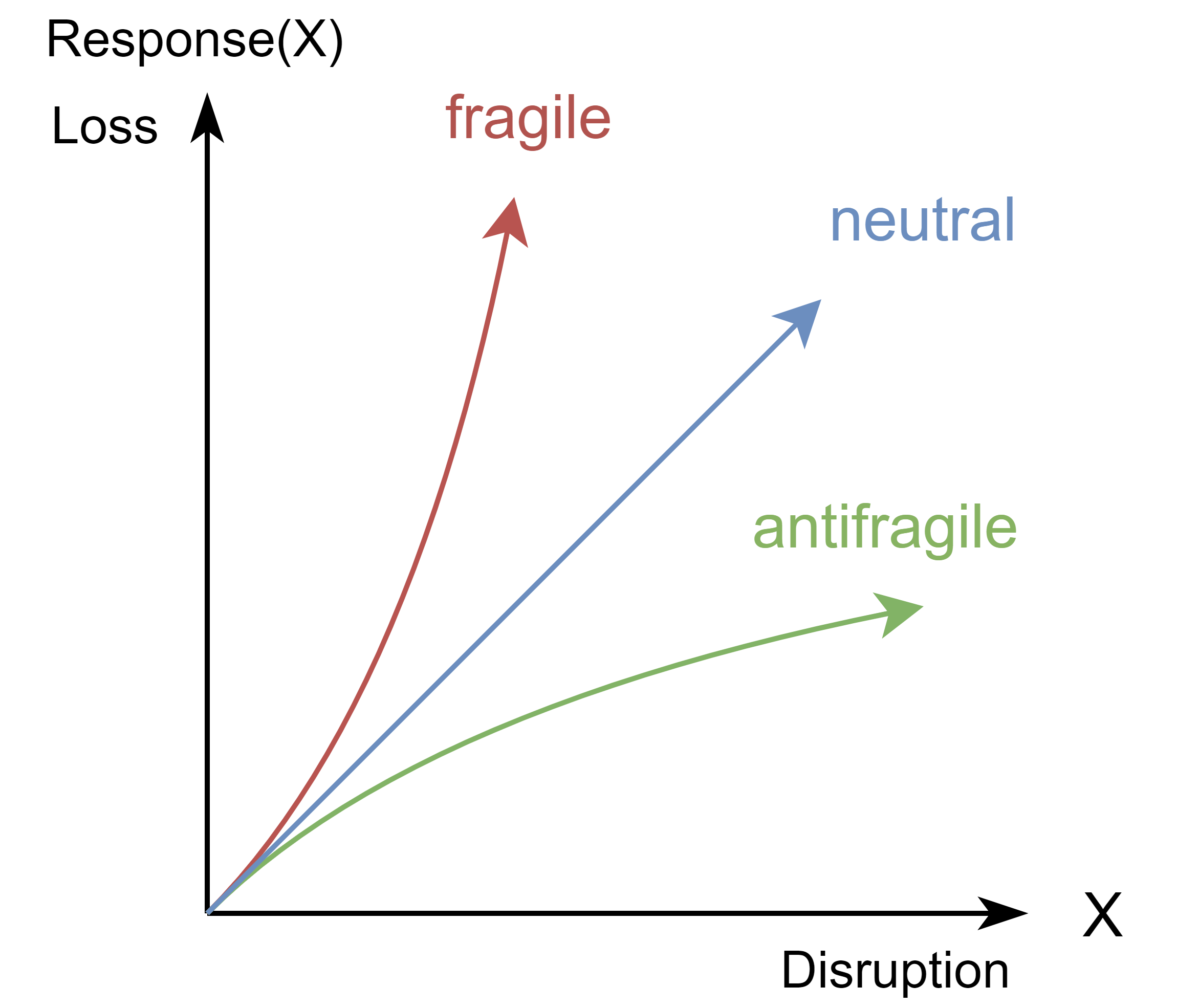
(a) Nonlinear relationship for a continuous function

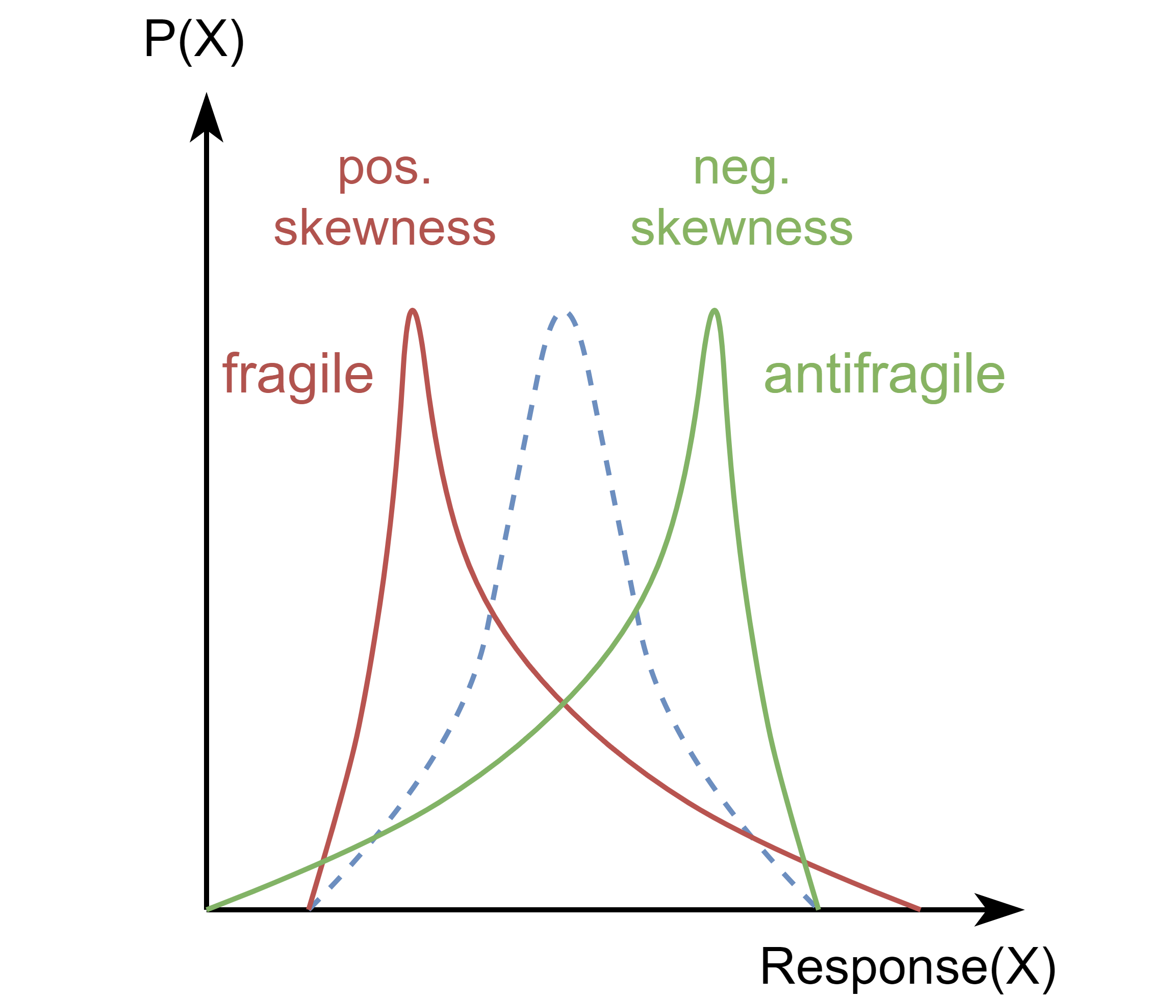
(b) Distribution skewness for discrete measurements

Figure 3: Characteristics and identification of (anti-)fragility

In this paper, we address three sets of opposing concepts for the mathematical analysis when studying the fragile nature of road transportation systems:

• microscopic / macroscopic

• demand disruption / supply disruption

• onset of disruption / recovery from disruption

As microscopic and macroscopic traffic models were introduced in the previous Section 2, here we start with differentiating between demand and supply disruptions, with the latter sometimes referred to as MFD disruptions. Since traffic networks primarily involve the management of supply and demand, we consider that any traffic disruption in the real world can be classified as either a demand or a supply disruption. A demand disruption can be easily understood as, for example, surging traffic due to a social event, whereas a supply disruption may indicate an impaired network due to external factors, such as adversarial weather or lane closure. Additionally, since disruptions represent abnormal cases that only exist temporarily, we consider not only the onset of disruptions but also assess the recovery process of the systems following such disruptions. This coincides with the aforementioned definitions of robustness and resilience, i.e., robustness is about resistance against disruptions while resilience is about the recovery from them. By considering both the onset and recovery processes, it becomes possible to compare the performance between either robust and antifragile designs or resilient and antifragile designs. The scheme of onset and recovery from demand or supply disruptions are illustrated in Fig. 4(a) and Fig. 4(b), and since FDs share similar profiles as MFDs, we simply use MFDs here as examples for illustration. We denote the FD/MFD profile as $G(k)$ and assume a constant base demand in the network as $q$, resulting in an equilibrium traffic state in the network in the absence of any disruption. The initial density at equilibrium, the critical density, the new density after disruption, and the gridlock density are denoted as $k_{0}$, $k_{c}$, $k^{\prime}$, and $k_{\rm max}$, respectively. For the study of supply disruptions, we introduce a disruption magnitude coefficient, denoted as $r$, so that the disrupted MFD profile can be represented as $(1-r)G(k)$. It should also be noted that on the network level, instead of traffic flow - density, MFD can also be represented with vehicle accumulation - trip completion, such as in Zhou and Gayah (2021); Kouvelas et al. (2017); Genser and Kouvelas (2022). Hence, with vehicle accumulation denoted as $n$, $k_{*}$ and $G(k)$ can also be replace with $n_{*}$ and trip completion $G(n)$.

(a) Onset and recovery of a demand disruption

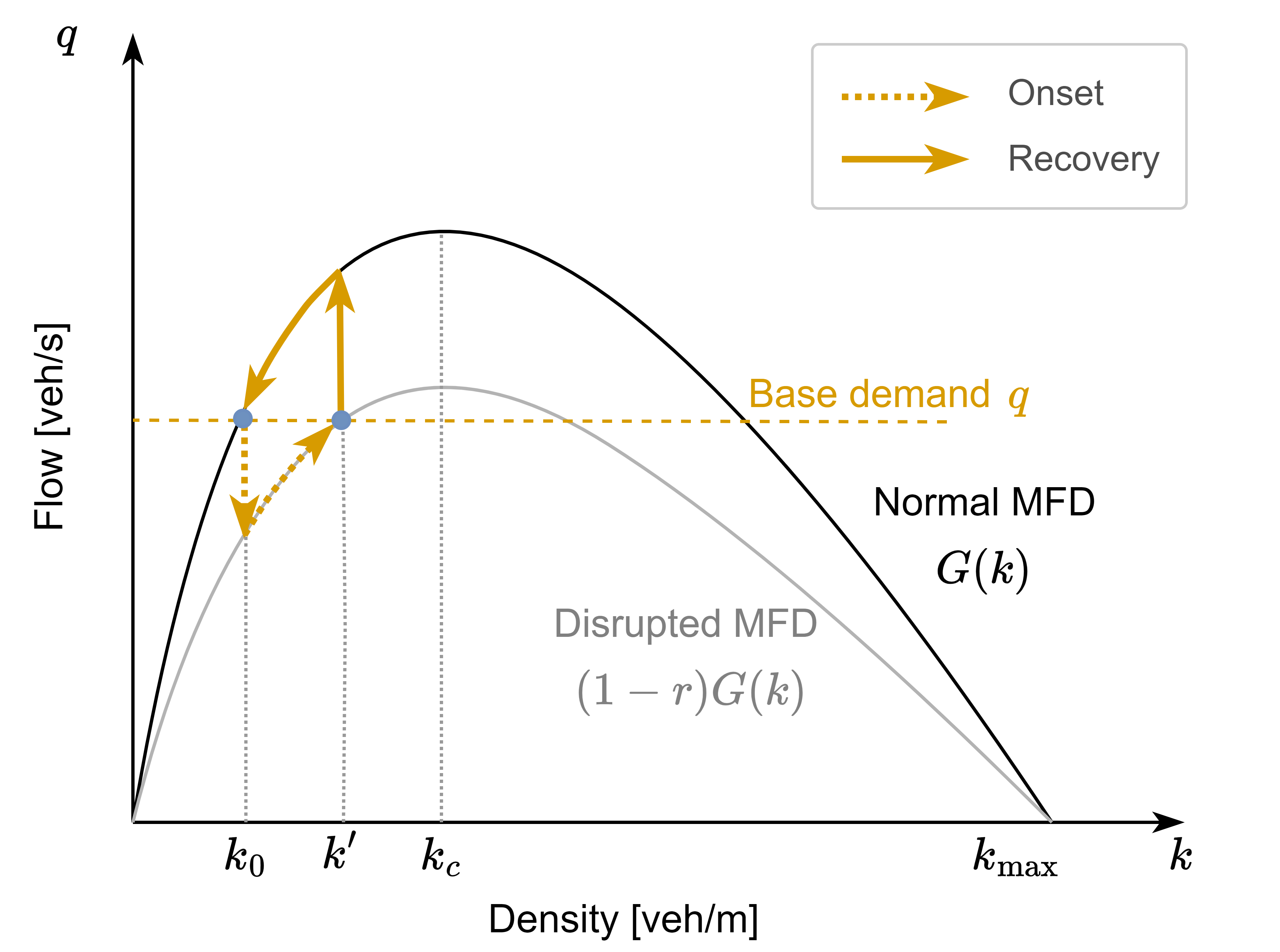
(b) Onset and recovery of a supply disruption

Figure 4: Onset and recovery of disruptions

Several assumptions need to be established to define the scope of our work. Also, as the study of fragility involves the recovery process from disruptions, a critical condition to avoid here is the network succumbing to a complete gridlock, where recovery is not possible anymore.

Assumption 1.

We study the onset of disruptions focusing only on the two stable traffic states before and after the disruptions, while the recovery is regarded as a gradual process of congestion dissipation.

For the onset of demand disruptions, we assume a rapid influx of traffic into the network, which can be characterized as an instantaneous event. For the onset of supply disruptions, although it may take some time for the number of vehicles within the network to accumulate, we understand it as a change from one stable traffic state $G(k_{0})$ to the final stable state $(1-r)G(k^{\prime})$, i.e., the equilibrium points in blue as shown in Fig. 4(b). The process of recovery from demand or supply disruptions, on the other hand, takes significantly longer as it is a traffic unloading and congestion dissipation process instead of an instantaneous event.

Assumption 2.

For demand disruptions, we assume $k^{\prime}>k_{c}$, whereas $k^{\prime}<k_{c}$ for supply disruptions.

A surging demand should be considered a disruption only when its presence leads to a reduction in the network’s maximal possible serviceability, i.e., causing the traffic state to enter the congested zone of the MFD and the flow is below the network capacity. On the other hand, for supply disruption with the constant base demand, if the traffic state can ever surpass the maximal capacity of the disrupted MFD profile, indicating the incoming flow is even greater than the maximal capacity of the network after supply disruptions, then the traffic density will continue to accumulate until the network reaches a full gridlock, and there will be no equilibrium point in this case after a disruption, violating Assumption 1.

Assumption 3.

For demand disruptions, we assume $q<G(k^{\prime})$, whereas $q<(1-r)G(k_{c})$ for supply disruptions.

Likewise, the necessity of this assumption also lies in the avoidance of gridlock for both demand and supply disruptions. If the base demand is higher than the outgoing flow after a demand disruption or the maximal capacity of the network after a supply disruption, then the traffic state will continue to move to complete gridlock.

4 Mathematical analysis of the fragility of road transportation systems

In this section, we conduct a mathematical analysis to evaluate the potential fragility of road transportation systems at both microscopic and macroscopic levels. The structure of this section is summarized in Table 1. The reason for not considering the recovery process on the microscopic level is that researchers rarely use FDs to study the recovery from congestion on a link level. And even if we do so, we can also easily get the same conclusion with Proposition 3 and or Proposition 6. In the subsequent study, to investigate the instantaneous disruption onset and between different stable states, the Average Time Spent (ATS) serves as the indicator for the overall performance of a link or a network, since ATS remains constant at any stable traffic state. Conversely, for the examination of disruption recovery, we use Total Time Spent (TTS), as applied in Zhou and Gayah (2021); Chen et al. (2022); Rodrigues and Azevedo (2019), to better reflect the temporal costs for all vehicles in the process, considering that the time spent in the network varies significantly for vehicles entering at different times.

Table 1: Structure of the mathematical proof

Disruption	Demand		Supply
	Micro	Macro	Micro	Macro
Onset	Proposition 1	Proposition 2	Proposition 4	Proposition 5
Recovery	-	Proposition 3	-	Proposition 6

4.1 Demand disruption

As outlined in Section 3, the presence of a positive second derivative in performance loss concerning the magnitude of disruption serves as an indication of the transportation system’s fragility, therefore, to illustrate the system’s fragility to demand disruption, we analyze the derivatives of time spent, i.e., ATS for the onset of disruptions or TTS for the recovery process, relative to the initial disruption demand, either represented by disruption density $k^{\prime}$ or an initial disruption demand $n^{\prime}$ when we study the relationship between trip completion and vehicle accumulation. If the system is neither fragile nor antifragile, this approach is expected to yield a linearly growing loss in performance alongside the disruption and zero derivatives. Quoting and in line with the famous statistician George Box, “All models are wrong, but some are useful,” we employ both a numerical and an analytical FD/MFD to investigate the fragile properties under the onset of demand disruption at both microscopic and macroscopic scales.

Proposition 1.

Road transportation systems are fragile with the onset of demand disruptions on the microscopic level.

Proof.

We choose the second-degree polynomial FD in Greenshields et al. (1934) as the numerical traffic model and the two-regime linear FD Daganzo (1994) as the analytical traffic model.

For the Greenshields second-degree polynomial FD, the following equations describe traffic in a stable state with $a$ and $b$ being the polynomial coefficients. The traffic flow $q$ and average speed $v$ can be determined as in Eq. 2 and Eq. 3, with the speed-density profile shown in Fig. 5(a).

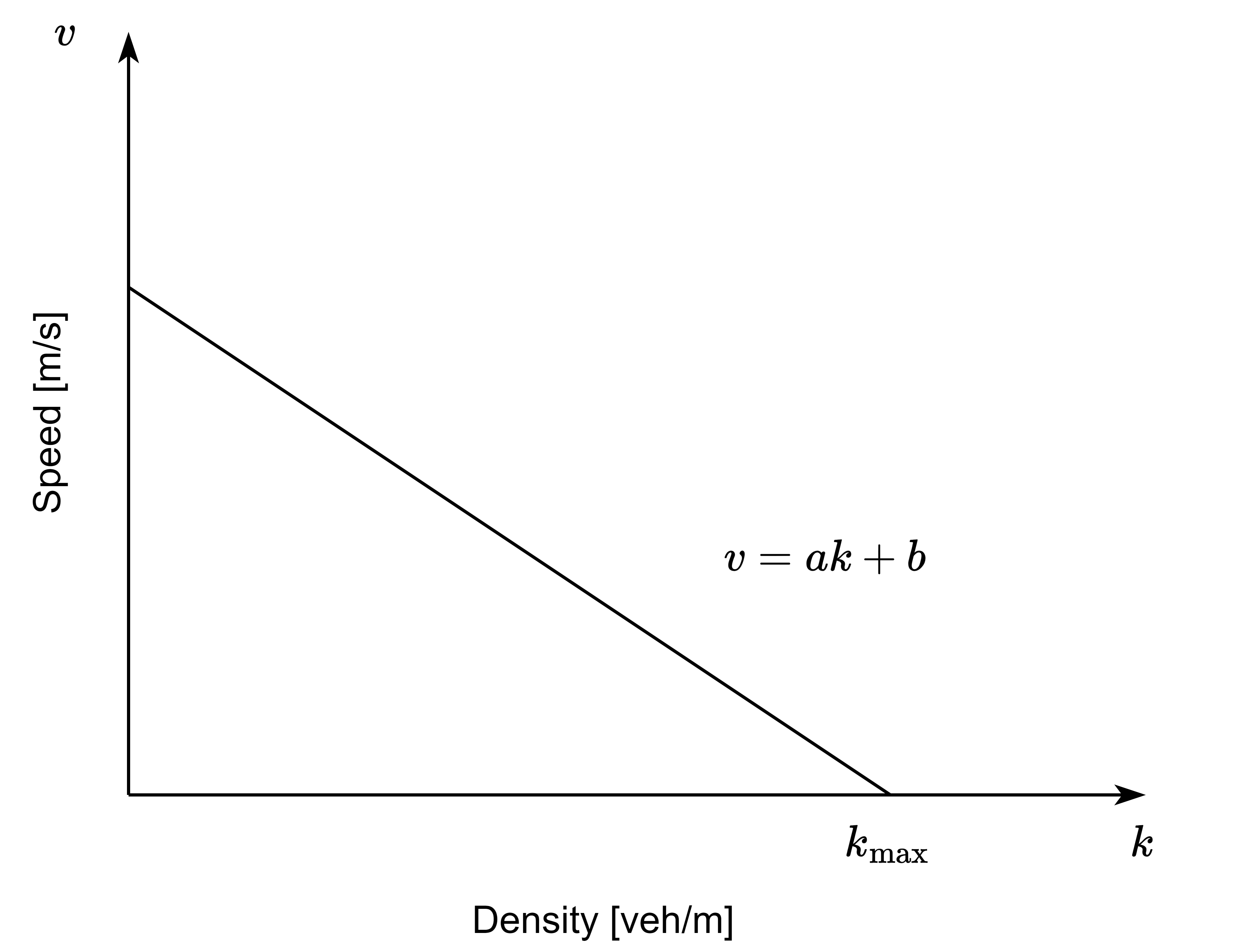
(a) Greenshields speed-density FD

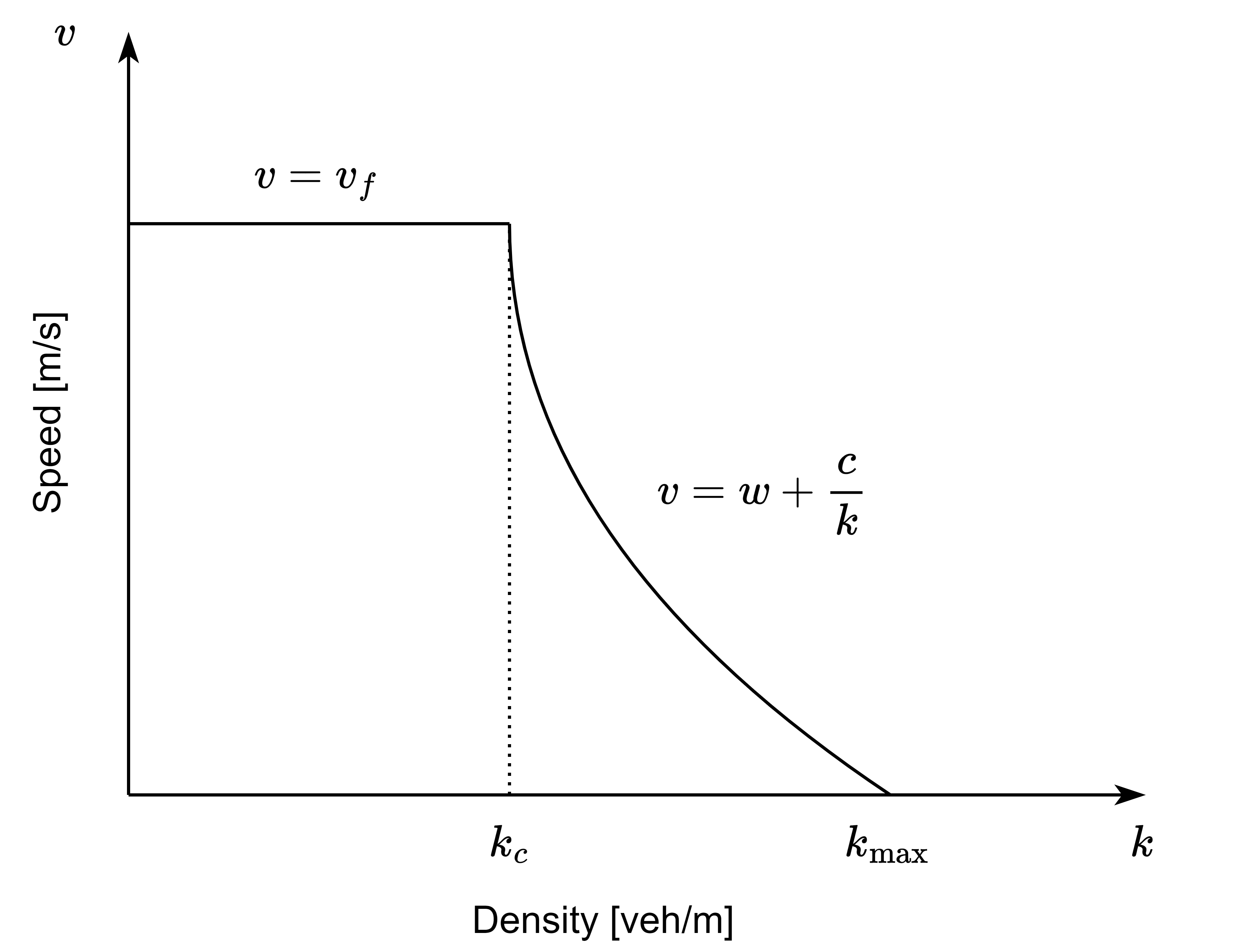
(b) Daganzo speed-density FD

Figure 5: Mathematical models of speed-density FDs

$$G(k) =ak^{2}+bk$$ (2)

$$v(k) =\frac{q}{k}=ak+b$$ (3)

With the sudden onset of a demand disruption $k^{\prime}$, for a link with a given length of $L$, the ATS and its first and second derivatives over such disruption density $k^{\prime}$ are:

$$ATS =\frac{L}{v(k^{\prime})}=\frac{L}{ak^{\prime}+b}$$ (4)

$$\frac{dATS}{dk^{\prime}} =-aL(ak^{\prime}+b)^{-2}$$ (5)

$$\frac{d^{2}ATS}{dk^{\prime 2}} =2a^{2}L(ak^{\prime}+b)^{-3}$$ (6)

Since the coefficient $a$ is negative and the physical meaning of the term $ak^{\prime}+b$ is the average speed of vehicles on this link, which should always be positive unless in gridlock, thus, both the first and second derivatives of ATS over $k^{\prime}$ are positive, indicating the fragility of transportation systems on a microscopic level.

In the Daganzo two-regime linear model, the speed-density FD can be formulated as the following Eq. 7, as shown in Fig. 5(b).

$$v(k)=\begin{cases}v_{f},&0\leq k<k_{c}\\ w+\frac{c}{k},&k_{c}\leq k\leq k_{\rm max}\end{cases}$$ (7)

When the disruption density $k^{\prime}$ is below the critical density $k_{c}$, the ATS and its first and second derivatives are:

$$ATS=\frac{L}{v_{f}}$$ (8)

$$\frac{dATS}{dk^{\prime}}=0$$ (9)

$$\frac{d^{2}ATS}{dk^{\prime 2}}=0$$ (10)

With the second derivative being zero, it indicates the traffic states before $k_{c}$ are neither fragile nor antifragile. However, as per Assumption 2, the congested area of the MFD is the study focus for demand disruptions, so now we study the derivatives when $k^{\prime}$ is over $k_{c}$:

$$ATS =\frac{L}{v(k^{\prime})}=\frac{L}{w+\frac{c}{k^{\prime}}}$$ (11)

$$\frac{dATS}{dk^{\prime}} =\frac{cL}{(wk^{\prime}+c)^{2}}$$ (12)

$$\frac{d^{2}ATS}{dk^{\prime 2}} =\frac{-2wcL}{(wk^{\prime}+c)^{3}}$$ (13)

Before the disruption density $k^{\prime}$ reaches the maximal density $k_{\rm max}$ of this link, $wk^{\prime}+c>0$ always holds true, and since $w<0$ as well as $c>0$, therefore, both the first and second derivatives are positive.

∎

Proposition 2.

Road transportation systems are fragile with the onset of demand disruptions on the macroscopic level.

Proof.

Likewise, on the macroscopic level, we study the fragile property based on the third-degree polynomial MFD in Geroliminis et al. (2013) and multi-regime linear MFD based on MoC in Daganzo and Geroliminis (2008). For MFD approximated with a third-degree polynomial, similar to the Greenshields FD in Eq. 2, we have:

$$G(k) =ak^{3}+bk^{2}+ck$$ (14)

$$v(k) =\frac{q}{k}=ak^{2}+bk+c$$ (15)

Consequently, the ATS and its first and second derivatives are:

$$ATS =\frac{L}{v(k^{\prime})}=\frac{L}{ak^{\prime 2}+bk^{\prime}+c}$$ (16)

$$\frac{dATS}{dk^{\prime}} =\frac{-(2ak^{\prime}+b)L}{(ak^{\prime 2}+bk^{\prime}+c)^{2}}$$ (17)

$$\frac{d^{2}ATS}{dk^{\prime 2}} =\frac{\frac{3}{2}(2ak^{\prime}+b)^{2}+\frac{1}{2}(b^{2}-4ac)}{(ak^{\prime 2}+bk^{\prime}+c)^{3}}L$$ (18)

The average speed has to be a real number, indicating Eq. 15 should have real roots, so $b^{2}-4ac>0$ should hold true. Therefore, the derivatives are positive.

The MFD derived with MoC can be approximated by a series of linear functions. Likewise to the Daganzo two-regime linear FD as in Eq. 13, for any linear function, the second derivative is:

$$\frac{d^{2}ATS}{dk^{\prime 2}} =\frac{-2u_{i}c_{i}L}{(u_{i}k^{\prime}+c_{i})^{3}}$$ (19)

As coefficient $c_{i}$ is positive for any cut since the y-intercept should always be positive by definition of MoC, whether the second derivative is positive or negative depends solely on $u_{i}$. The cuts that intercept the MFD before the critical density $k_{c}$ exhibit antifragile properties ($u_{i}>0$, in blue as shown in Fig. 6) while the others with intercepts larger than the critical density $k_{c}$ show fragile responses ($u_{i}<0$, in red), with an exception in case there’s a cut at the critical density ($u_{i}=0$, in gray). Conforming to Assumption 2, for demand disruptions, we focus on the cuts with intercepts larger than the critical density $k_{c}$ ($u_{i}<0$). The second derivative for these cuts is positive indicating a fragile property.

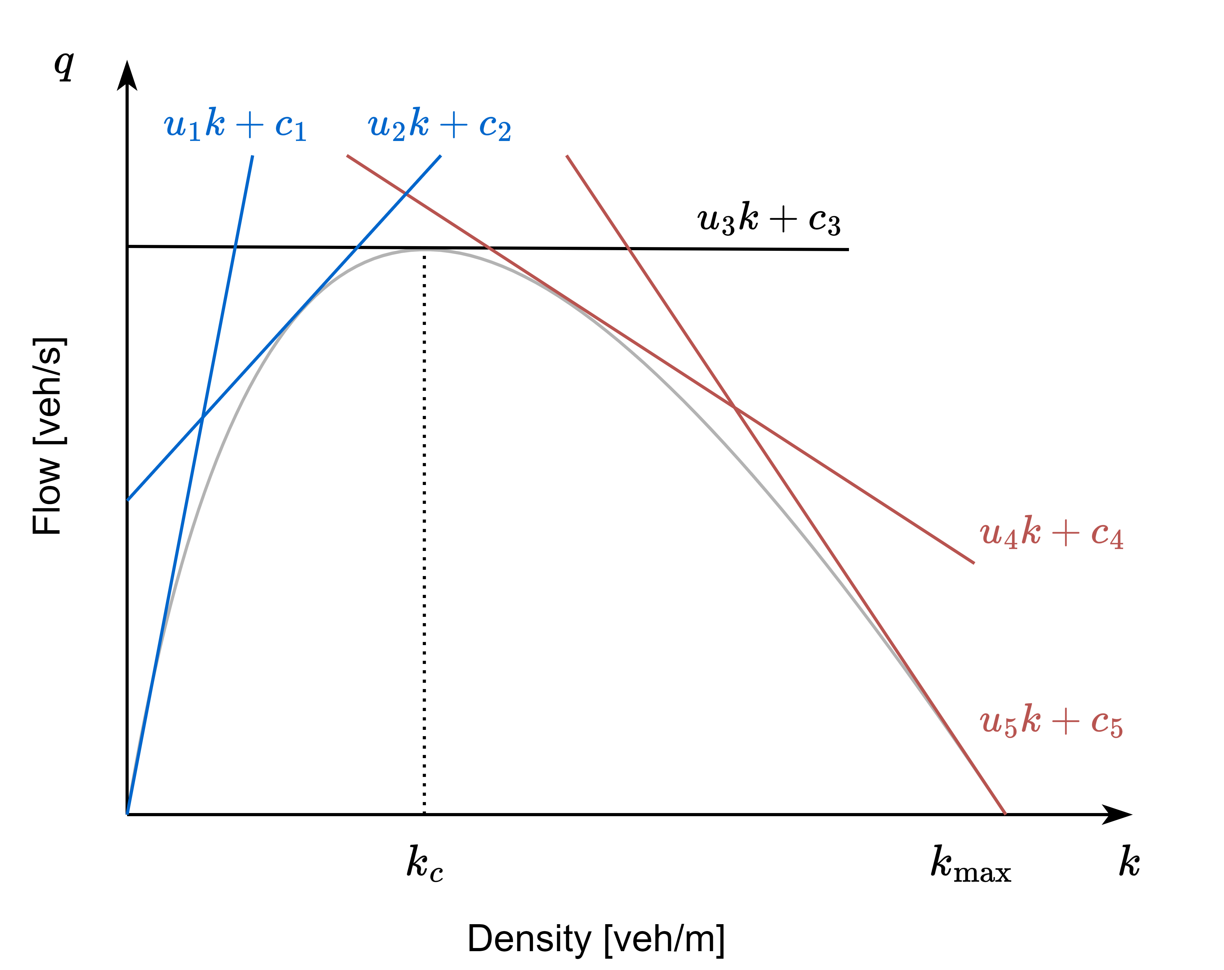
Figure 6: Daganzo multi-regime linear MFD

∎

Proposition 3.

Road transportation systems are fragile when going through the recovery process from demand disruptions.

Proof.

According to Assumption 1, we simplify this surging demand as a disruption that takes place instantly in the network, denoted as $n^{\prime}$ at time $t^{\prime}=0$. As the MoC is composed of a series of linear functions with decreasing gradients as the vehicle accumulation increases, the multi-linear regimes can be represented into multiple sets of consecutive duo linear functions as Fig. 7 shows. The four constants $a_{1}$, $a_{2}$, $b_{1}$, and $b_{2}$ are the slope and y-intercept on the coordinates for the two cuts, with $a_{2}>a_{1}$ and $b_{1}>b_{2}>0$. We refer to these two linear functions as the more congested branch and the less congested branch. Also, the critical accumulation $n_{c}$ here does not represent the critical point of the entire MFD, but rather the critical accumulation of any two consecutive cuts. After a certain period $t_{c}$, the number of vehicles in the network reaches this critical accumulation $n_{c}$. And after any period $t>t_{c}$, the vehicle accumulation becomes $n$. We also denote the initial trip completion and critical trip completion as $m_{0}=a_{1}n^{\prime}+b_{1}$ and $m_{c}=a_{1}n_{c}+b_{1}=a_{2}n_{c}+b_{2}$ respectively.

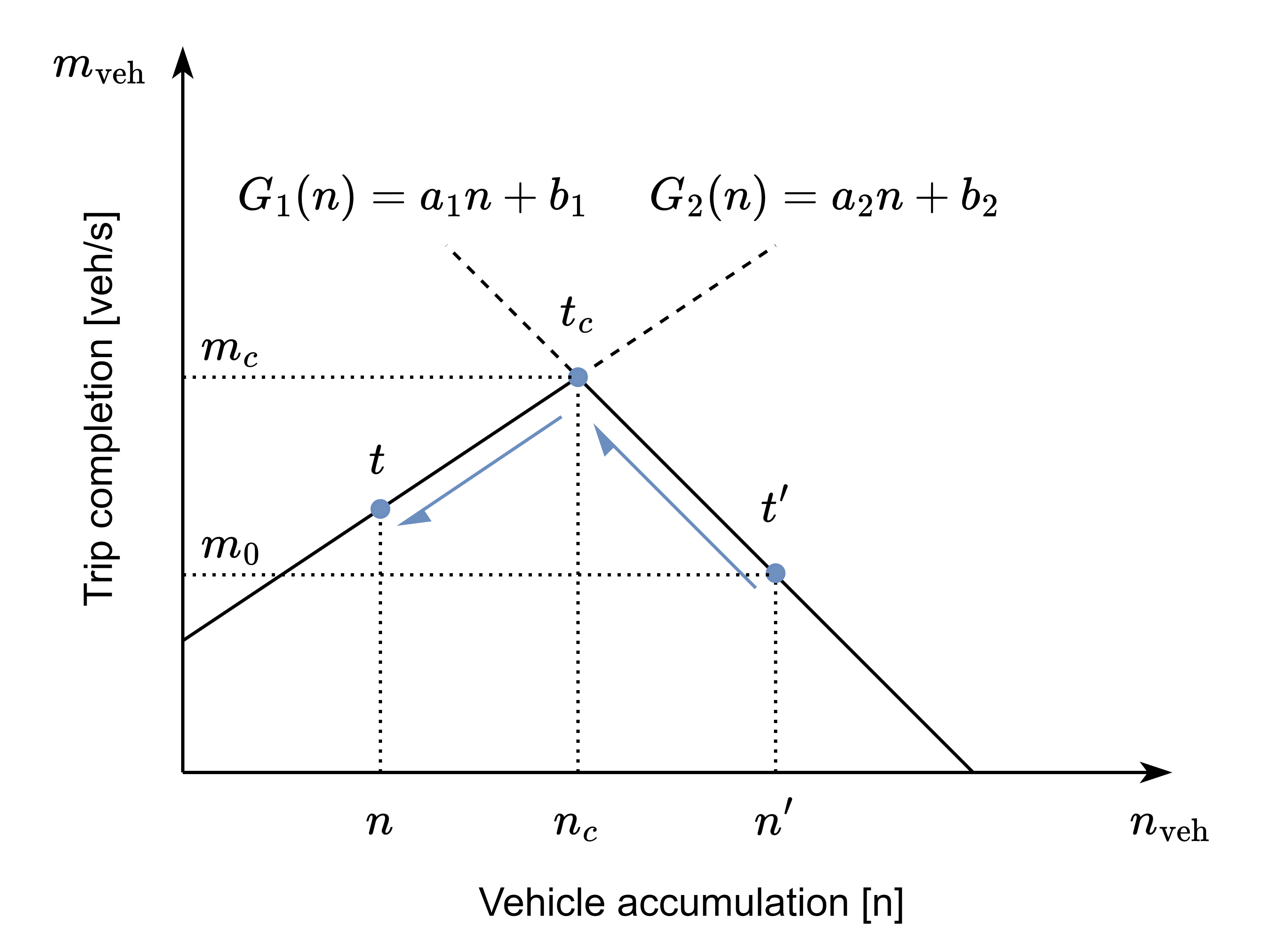
Figure 7: Simplification of MoC

Any two consecutive cuts of the MFD can be formulated into the following Eq. 20:

$$G(n)=\begin{cases}a_{1}n+b_{1},&n_{c}\leq n<n_{\rm max}\\ a_{2}n+b_{2},&0\leq n<n_{c}\end{cases}$$ (20)

The system dynamics can be summarized as the following Eq. 21.

$$\frac{dn}{dt}=-G(n)+q=-a_{i}n-b_{i}+q$$ (21)

When the traffic states move only along a single branch, and given any initial vehicle accumulation $n_{1}$ at the beginning of a period from $t_{1}$ to $t_{2}$, the number of vehicles $n_{2}$ at the end of this period can be determined as:

$$\int_{t_{1}}^{t_{2}}dt =-\int_{n_{1}}^{n_{2}}\frac{1}{a_{i}n+b_{i}-q}dn$$ (22)

$$t_{2}-t_{1} =-\frac{1}{a_{i}}\ln{\left(\frac{a_{i}n_{2}+b_{i}-q}{a_{i}n_{1}+b_{i}-q}\right)}$$ (23)

$$n_{2} =\frac{e^{-a_{i}(t_{2}-t_{1})}(a_{i}n_{1}+b_{i}-q)}{a_{i}}-\frac{b_{i}-q}{a_{i}}$$ (24)

Therefore, with the disruption accumulation $n^{\prime}$, and when the traffic states are on the same branch. After any time $t$, the vehicle accumulation $n$ would be:

$$n =\frac{a_{1}n^{\prime}+b_{1}-q}{a_{1}}e^{-a_{1}t}-\frac{b_{1}-q}{a_{1}}$$ (25)

The TTS in this case can be calculated as:

$$TTS=\int_{0}^{t}ndt =\int_{0}^{t}\left(\frac{a_{1}n^{\prime}+b_{1}-q}{a_{1}}e^{-a_{1}t}-\frac{b_{1}-q}{a_{1}}\right)dt$$ (26)

$$=-\frac{a_{1}n^{\prime}+b_{1}-q}{a_{1}^{2}}e^{-a_{1}t}-\frac{b_{1}-q}{a_{1}}t+\frac{a_{1}n^{\prime}+b_{1}-q}{a_{1}^{2}}$$ (27)

Now we calculate the derivatives of TTS considering $t$ as any positive constant.

$$\frac{dTTS}{dn^{\prime}} =\frac{1}{a_{1}}-\frac{e^{-a_{1}t}}{a_{1}}$$ (28)

$$\frac{d^{2}TTS}{dn^{\prime 2}} =0$$ (29)

The second derivative of TTS is $0$, indicating that when the traffic states move only along a single branch, it shows neither fragility nor antifragility.

On the other hand, when the traffic state goes over the critical vehicle accumulation $n_{c}$, and since the MoC is a piecewise function, we calculate the TTS separately on both the more congested and the less congested branches, denoted as $TTS_{1}$ and $TTS_{2}$. Since the critical time $t_{c}$ is still unknown, we need to determine $t_{c}$ first, similar to Eq. 23.

$$t_{c} =-\frac{1}{a_{1}}\ln{\left(\frac{a_{1}n_{c}+b_{1}-q}{a_{1}n^{\prime}+b_{1}-q}\right)}$$ (30)

As both $a_{1}n_{c}+b_{1}$ and $a_{2}n_{c}+b_{2}$ are equal to $m_{c}$, we can rewrite the above Eq. 30 as:

$$t_{c} =-\frac{1}{a_{1}}\ln{\left(\frac{m_{c}-q}{a_{1}n^{\prime}+b_{1}-q}\right)}$$ (31)

Likewise to Eq. 27, the $TTS_{1}$ for the more congested branch is:

$$TTS_{1} =-\frac{a_{1}n^{\prime}+b_{1}-q}{a_{1}^{2}}e^{-a_{1}t_{c}}-\frac{b_{1}-q}{a_{1}}t_{c}+\frac{a_{1}n^{\prime}+b_{1}-q}{a_{1}^{2}}$$ (32)

$$=-\frac{m_{c}-q}{a_{1}^{2}}+\frac{b_{1}-q}{a_{1}^{2}}\ln{\left(\frac{m_{c}-q}{a_{1}n^{\prime}+b_{1}-q}\right)}+\frac{a_{1}n^{\prime}+b_{1}-q}{a_{1}^{2}}$$ (33)

Since TTS is the sum of $TTS_{1}$ and $TTS_{2}$, the second derivative of TTS would also be the sum of the derivatives. The derivatives for $TTS_{1}$ are:

$$\frac{dTTS_{1}}{dn^{\prime}} =-\frac{b_{1}-q}{a_{1}}(a_{1}n^{\prime}+b_{1}-q)^{-1}+\frac{1}{a_{1}}$$ (34)

$$\frac{d^{2}TTS_{1}}{dn^{\prime 2}} =(b_{1}-q)(a_{1}n^{\prime}+b_{1}-q)^{-2}$$ (35)

According to Eq. 24, the vehicle accumulation on the less congested branch from $t_{c}$ to $t$ would be:

$$n =\frac{e^{-a_{2}(t-t_{c})}(a_{2}n_{c}+b_{2}-q)}{a_{2}}-\frac{b_{2}-q}{a_{2}}$$ (36)

$$=\frac{e^{a_{2}t_{c}}(m_{c}-q)}{a_{2}}e^{-a_{2}t}-\frac{b_{2}-q}{a_{2}}$$ (37)

The $TTS_{2}$ for the less congested branch would be:

$$TTS_{2}=\int_{t_{c}}^{t}ndt =\int_{t_{c}}^{t}\left(\frac{e^{a_{2}t_{c}}(m_{c}-q)}{a_{2}}e^{-a_{2}t}-\frac{b_{2}-q}{a_{2}}\right)dt$$ (38)

$$=-\frac{e^{-a_{2}t}(m_{c}-q)}{a_{2}^{2}}e^{a_{2}t_{c}}+\frac{b_{2}-q}{a_{2}}t_{c}+\frac{m_{c}-q}{a_{2}^{2}}-\frac{b_{2}-q}{a_{2}}t$$ (39)

The derivatives on the less congested branch are:

$$\frac{dTTS_{2}}{dn^{\prime}} =-\frac{(m_{c}-q)^{1-\frac{a_{2}}{a_{1}}}e^{-a_{2}t}}{a_{2}}(a_{1}n^{\prime}+b_{1}-q)^{\frac{a_{2}}{a_{1}}-1}+\frac{b_{2}-q}{a_{2}}(a_{1}n^{\prime}+b_{1}-q)^{-1}$$ (40)

$$\frac{d^{2}TTS_{2}}{dn^{\prime 2}} =-\left(\frac{(a_{2}-a_{1})(m_{c}-q)^{1-\frac{a_{2}}{a_{1}}}e^{-a_{2}t}}{a_{2}}(a_{1}n^{\prime}+b_{1}-q)^{\frac{a_{2}}{a_{1}}}+\frac{a_{1}(b_{2}-q)}{a_{2}}\right)(a_{1}n^{\prime}+b_{1}-q)^{-2}$$ (41)

The second derivative of the whole process can be written as:

$$\frac{d^{2}TTS}{dn^{\prime 2}} =\frac{d^{2}TTS_{1}}{dn^{\prime 2}}+\frac{d^{2}TTS_{2}}{dn^{\prime 2}}$$ (42)

$$=\left(b_{1}-q-\frac{e^{-a_{2}t}}{a_{2}}(a_{2}-a_{1})(m_{c}-q)^{1-\frac{a_{2}}{a_{1}}}(m_{0}-q)^{\frac{a_{2}}{a_{1}}}-\frac{a_{1}(b_{2}-q)}{a_{2}}\right)(m_{0}-q)^{-2}$$ (43)

As per Assumption 3, we have $m_{0}-q>0$, so if a transportation system is to be fragile, $d^{2}TTS/dn^{\prime 2}$ should also be positive, and the following equation has to be true:

$$b_{1}-q-\frac{e^{-a_{2}t}}{a_{2}}(a_{2}-a_{1})(m_{c}-q)^{1-\frac{a_{2}}{a_{1}}}(m_{0}-q)^{\frac{a_{2}}{a_{1}}}-\frac{a_{1}(b_{2}-q)}{a_{2}}>0$$ (44)

Since $t>t_{c}$ and $a_{2}>a_{1}$, regardless of whether $a_{2}$ is positive or negative, the following relationship always holds:

$$-\frac{e^{-a_{2}t}}{a_{2}}>-\frac{e^{-a_{2}t_{c}}}{a_{2}}$$ (45)

As the following three terms, $a_{2}-a_{1}$, $(m_{c}-q)^{1-\frac{a_{2}}{a_{1}}}$, and $(m_{0}-q)^{\frac{a_{2}}{a_{1}}}$ are all positive, the following relationship is true:

$$b_{1}-q-\frac{e^{-a_{2}t}}{a_{2}}(a_{2}-a_{1})(m_{c}-q)^{1-\frac{a_{2}}{a_{1}}}(m_{0}-q)^{\frac{a_{2}}{a_{1}}}-\frac{a_{1}(b_{2}-q)}{a_{2}}>$$ (46)

$$b_{1}-q-\frac{e^{-a_{2}t_{c}}}{a_{2}}(a_{2}-a_{1})(m_{c}-q)^{1-\frac{a_{2}}{a_{1}}}(m_{0}-q)^{\frac{a_{2}}{a_{1}}}-\frac{a_{1}(b_{2}-q)}{a_{2}}$$ (47)

Here we substitute $t_{c}$ in Eq. 47 with Eq. 31 and we get:

$$b_{1}-q-\frac{(a_{2}-a_{1})(m_{c}-q)}{a_{2}}-\frac{a_{1}(b_{2}-q)}{a_{2}} =$$ (48)

$$a_{1}\left(\frac{b_{1}-m_{c}}{a_{1}}-\frac{b_{2}-m_{c}}{a_{2}}\right)=a_{1}(n_{c}-n_{c}) =0$$ (49)

Hence, we have:

$$b_{1}-q-\frac{e^{-a_{2}t}}{a_{2}}(a_{2}-a_{1})(m_{c}-q)^{1-\frac{a_{2}}{a_{1}}}(m_{0}-q)^{\frac{a_{2}}{a_{1}}}-\frac{a_{1}(b_{2}-q)}{a_{2}}>0$$ (50)

The second derivative of TTS over the disruption vehicle accumulation $n^{\prime}$ is positive, which indicates the fragility. ∎

4.2 Supply disruption

While a positive second derivative of ATS or TTS on traffic demand signifies the fragility of the road transportation network to demand disruptions, establishing a positive second derivative of time spent concerning the magnitude of FD/MFD disruption would demonstrate the fragility from the perspective of supply disruptions. Here we use a supply disruption magnitude coefficient $r$ and the disrupted FD/MFD is expressed as $(1-r)G(n)$. Although real-world MFD may be decreased in various shapes, we use this simple approach as applied in Ambühl et al. (2020) when studying the uncertainties of MFDs. The physical meaning of $(1-r)G(n)$ relates to the decrease of the free-flow speed due to, e.g., snowy weather and icy roads, with the maximal density of the network remaining unchanged. The traffic demand at equilibrium before the MFD disruption is $q=G(k_{0})$, or $q=G(n_{0})$. After the supply disruption, as per Assumption 3, the supply disruption magnitude coefficient $r\in[0,1)$ is not significantly large so the traffic demand remains below the maximal capacity on the disrupted MFD profile, and the new equilibrium point is $q=(1-r)G(k^{\prime}(r))$, or $q=(1-r)G(n^{\prime}(r))$. It should be noted that, unlike the study of demand disruption, when studying supply disruptions, $k^{\prime}(r)$ is a dependent variable on $r$.

Proposition 4.

Road transportation systems are fragile with the onset of supply disruptions on the microscopic level.

Proof.

First, we study the fragile properties of the road transportation systems under the onset of supply disruptions based on the microscopic model Greenshields FD. Here, the base demand $q$ is constant before and after the onset of the supply disruption, and can be used to build the relationship between the two stable states before and after the supply disruption.

$$q=G(k_{0})=(1-r)G(k^{\prime}(r))=(1-r)(ak^{\prime}(r)^{2}+bk^{\prime}(r))$$ (51)

So, the traffic density of the new equilibrium point after the MFD disruption would be:

$$k^{\prime}(r) =\frac{\sqrt{b^{2}+\frac{4aq}{1-r}}-b}{2a}$$ (52)

The $ATS$ and its first and second derivatives are:

$$ATS =\frac{L}{v(k^{\prime})}=\frac{Lk^{\prime}(r)}{q}=\frac{L}{2aq}((b^{2}+\frac{4aq}{1-r})^{\frac{1}{2}}-b)$$ (53)

$$\frac{dATS}{dr} =L(b^{2}(1-r)+4aq)^{-\frac{1}{2}}(1-r)^{-\frac{3}{2}}$$ (54)

$$\frac{d^{2}ATS}{dr^{2}} =\frac{b^{2}L}{2}(b^{2}(1-r)+4aq)^{-\frac{3}{2}}(1-r)^{-\frac{3}{2}}+\frac{3L}{2}(b^{2}(1-r)+4aq)^{-\frac{1}{2}}(1-r)^{-\frac{5}{2}}$$ (55)

As $k^{\prime}$ has a physical meaning of disruption density, so it should have real roots with $b^{2}+4aq/1-r$ being positive. And since $1-r>0$, therefore, $d^{2}ATS/dr^{2}$ is always positive and indicates the fragility property of transportation systems when faced with supply disruption on the microscopic level. Likewise to the proof of demand disruption, the Daganzo FD is a special case of the MoC, so we directly prove the fragility on the macroscopic level with MoC illustrated in the following section.

∎

Proposition 5.

Road transportation systems are fragile with the onset of supply disruptions on the macroscopic level.

Proof.

As the proof of fragility under supply disruption with cubic polynomial MFDs involves solving the roots for cubic equations, for simplicity reasons, we prove only with Daganzo MoC. Since the traffic demand $q$ is constant, the traffic density of the new stable state $k^{\prime}(r)$ would be:

$$q =(1-r)(uk^{\prime}(r)+c)$$ (56)

$$k^{\prime}(r) =\frac{\frac{q}{1-r}-c}{u}$$ (57)

And the ATS and its derivatives are:

$$ATS =\frac{Lk^{\prime}(r)}{q}=\frac{L}{qu}(\frac{q}{1-r}-c)$$ (58)

$$\frac{dATS}{dr} =\frac{L}{u}(1-r)^{-2}$$ (59)

$$\frac{d^{2}ATS}{dr^{2}} =\frac{2L}{u}(1-r)^{-3}$$ (60)

As per Assumption 2, when studying supply disruptions, we focus on the uncongested zone of the MFD, meaning the slope of these relevant cuts is positive so that both derivatives are positive.

∎

Proposition 6.

Road transportation systems are fragile when going through the recovery process from supply disruptions.

Proof.

To study the possible fragile properties of road transportation networks regarding the recovery process from supply disruptions, we need to combine the conclusions from Proposition 3 and Proposition 5. In Proposition 3, we’ve proven the recovery process to be fragile when the traffic state shifts from the more congested branch to the less congested branch for any two consecutive cuts on the Daganzo MFD, or to be neither fragile nor antifragile when it stays only on one single branch. Therefore, it can be mathematically summarized as $d^{2}TTS/dn^{\prime 2}\geq 0$. Following Assumption 2, $a_{1}>0$ holds as the branch is below the critical density, we can easily prove the first derivative $dTTS/dn^{\prime}$ to be non-negative as well with Eq. 34 and Eq. 40 through the same procedure as proving the second derivative to be positive. And for the proof of recovery from supply disruptions, as shown in Fig. 8, likewise to Proposition 5, the relationship between the original and new equilibrium points before and after MFD disruptions can be expressed as:

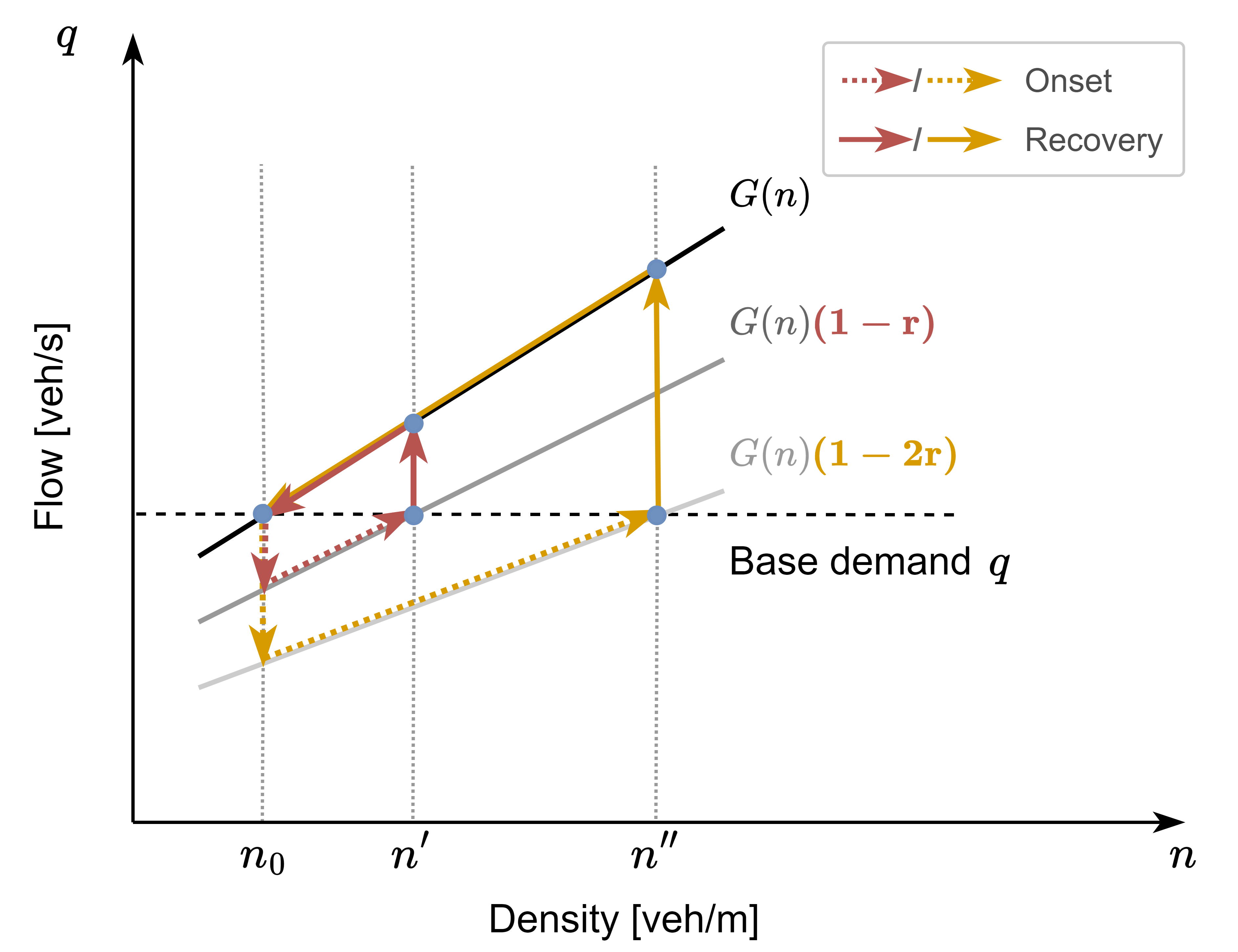
Figure 8: Recovery from supply disruption

$$q =un_{0}+c=(1-r)(un^{\prime}+c)$$ (61)

$$n^{\prime}(r) =\frac{un_{0}+c}{u(1-r)}-c/u$$ (62)

The first and second derivatives of $n^{\prime}$ over the supply disruption magnitude coefficient $r$ are:

$$\frac{dn^{\prime}}{dr} =\frac{un_{0}+c}{u}(1-r)^{-2}$$ (63)

$$\frac{d^{2}n^{\prime}}{dr^{2}} =\frac{2(un_{0}+c)}{u}(1-r)^{-3}$$ (64)

Since $u$ and $un_{0}+c$ are both positive, the derivatives of $n^{\prime}$ over $r$ are positive as well. Additionally, it can be easily proven that when considering the transition from a less congested to a more congested branch, the same conclusion also holds. As $TTS$ is a function of $n^{\prime}$ and $n^{\prime}$ is again a function of $r$, by applying the chain rule, we can get the second derivative of $TTS$ over $r$ as:

$$\frac{d^{2}TTS}{dr^{2}} =\frac{d}{dr}\left(\frac{dTTS}{dn^{\prime}}\cdot\frac{dn^{\prime}}{dr}\right)$$ (65)

$$=\frac{d^{2}TTS}{dn^{\prime 2}_{0}}\cdot\left(\frac{dn^{\prime}}{dr}\right)^{2}+\frac{dTTS}{dn^{\prime}}\cdot\frac{d^{2}n^{\prime}}{dr^{2}}$$ (66)

Because all the four components of the Eq. 66 have been demonstrated above to be non-negative, thus $d^{2}TTS/dr^{2}$ is also non-negative and we’ve proven the fragile nature of road transportation systems regarding the recovery process of supply disruptions.

∎

5 Numerical simulation

Even though researchers generally consider MFDs to be well-defined, road transportation systems in the real world and their MFDs are always subject to stochasticity all the time, as shown in Geroliminis and Daganzo (2008); Saffari et al. (2022); Ambühl et al. (2021), and this is the case for FDs as well (Qu et al., 2017; Siqueira et al., 2016). Therefore, when validating a newly proposed traffic control algorithm, it has become a common practice to account for model uncertainties and showcase the method’s robustness, such as in Geroliminis et al. (2013); Haddad and Mirkin (2017); Zhou and Gayah (2023). In our study, however, the model stochasticity cannot be directly reflected in the mathematical analysis, hence, it is indispensable to show the influence of realistic stochasticity on the fragile nature of transportation systems with a numerical simulation, i.e., whether the system still maintains the same fragile response under real-world errors in MFD when a demand or supply disruption is present.

In this section, we simulate the disruption recovery process. The MFD of the studied region is generated by applying MoC following Daganzo and Geroliminis (2008) with realistic parameters in the city center of Zurich. Some parameters, e.g., free-flow speed, back-propagation speed, maximal density, and capacity are provided in Ambühl et al. (2020) for Zurich with queried routes in Google API and with other validation methods. The total and average lane length for the city center is determined through SUMO with OpenStreetMap API. The average trip length of Zurich is studied in Schüssler and Axhausen (2008). We introduce stochasticity in the city center of Zurich with real traffic light data, which is publicized by the Statistical Office of Zurich and accessible in Genser et al. (2023). The authors acknowledge that MoC is developed with the premise of a homogeneous region, and given that the available data is limited to only one main intersection in this region, we assume that this intersection serves as a representative sample for the city center region. Also, since the signalization in Zurich is actuated based on the present traffic flow, they do not strictly follow a fixed-time signal cycle. Despite this actuation, a concentrated distribution can be easily observed in the dataset and we assume the green split of the cycle follows a normal distribution. The offset is considered to be zero in a way similar to the actuated signal in Yokohama in Daganzo and Geroliminis (2008). According to the daily average traffic density of Zurich in Ambühl et al. (2021), we approximate the traffic demand, which is also the trip completion when the traffic state is at equilibrium, is about $0.6veh/s$ for our studied region. This corresponds to an accumulation of around 975 vehicles in the city center. The parameters are summarized in Tab. 2.

Table 2: Estimated parameters for the city center of Zurich

Parameters	Notation	Unit	Value
Free-flow speed	$u_{0}$	$\rm m/s$	12.5
Back-propagation speed	$w_{0}$	$\rm m/s$	6.0
Maximal density	$\kappa$	$\rm veh/m$	0.145
Capacity	$s$	$\rm veh/s$	0.51
Total lane length	$D$	$\rm m$	68631
Average lane length	$l$	$\rm m$	167
Average trip length	$L$	$\rm m$	7110
Signal cycle time	$C$	$\rm s$	50
Signal green time (mean)	$\mu_{G}$	$\rm s$	14.8
Signal green time (std.)	$\sigma_{G}$	$\rm s$	2.5
Offset	$\delta$	$\rm s$	0
Traffic demand	$q$	$\rm veh/s$	0.6

As the average green time of the signal is 14.8 s and its standard deviation is 2.5 s, following the MoC described in Daganzo and Geroliminis (2008), we can produce three groups of cuts with the interval of one standard deviation, i.e., the green time being $\mu_{G}-\sigma_{G}$, $\mu_{G}$, or $\mu_{G}+\sigma_{G}$, and each group of cuts contains at least three cuts, as Fig. 9 shows. The group of cuts with a longer green time of signalization yields a greater MFD, and vice versa. The MFDs share the same maximal vehicle density of around 0.145 veh/m, which corresponds to a maximal accumulation of about 10000 vehicles for the studied region.

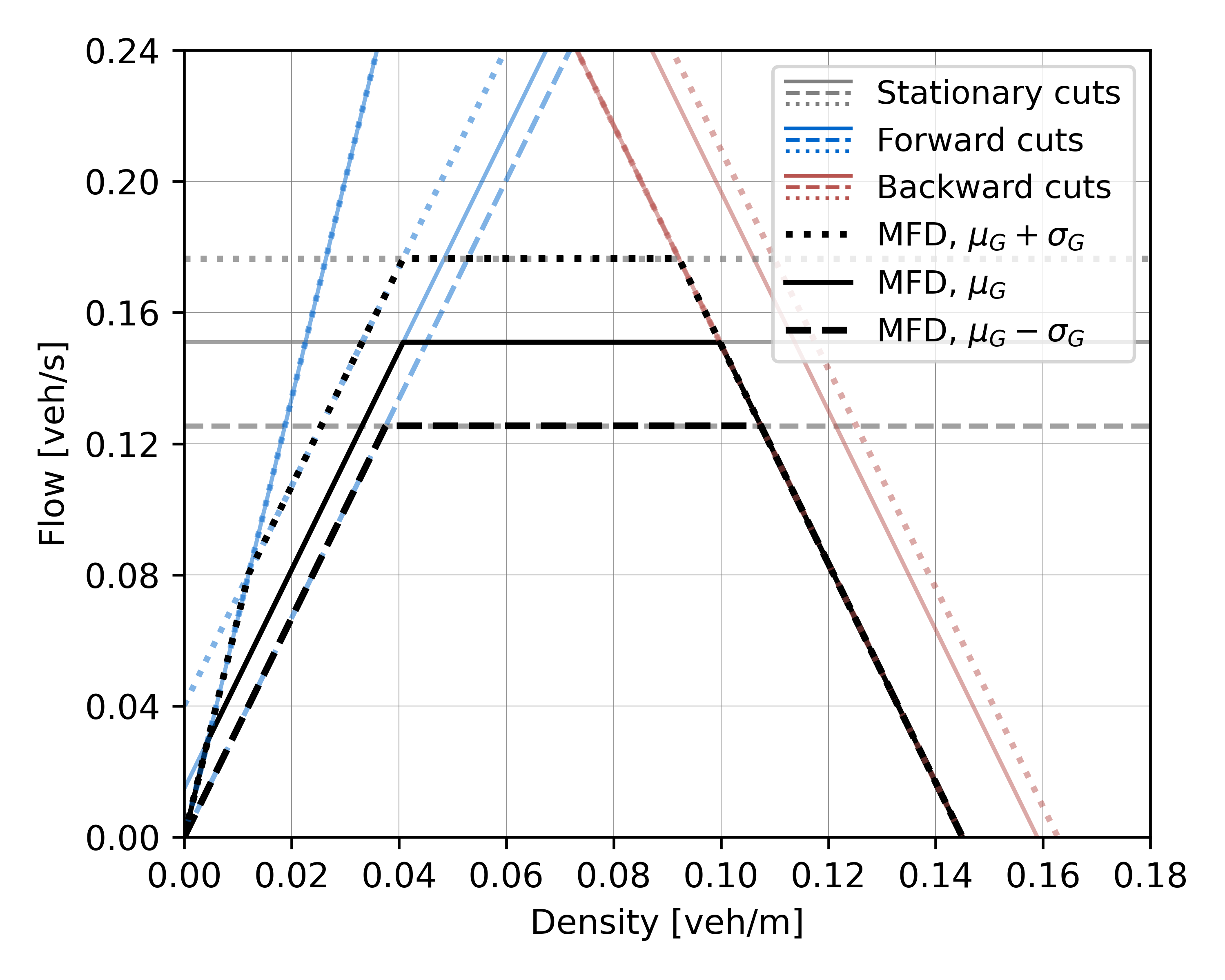
Figure 9: The MFD of the city center of Zurich through MoC

Now we start the numerical simulation with different initial disruption demands $n^{\prime}$ from 1000 to 8000 vehicles. The simulation time is 7200 seconds for each scenario with different initial demands. Fig. 10(a) demonstrates that TTS grows exponentially with linearly increasing initial disruption demand, which validates the fragile nature proved with mathematical analysis. The solid, dashed, or dotted line each represents the TTS calculated under the three deterministic MFDs with green time being $\mu_{G}$, $\mu_{G}-\sigma_{G}$, or $\mu_{G}+\sigma_{G}$. Other than the black curves, there are also 1000 scattering points forming the blue curve. Each scatter point is composed of a full disruption recovery process sampled with equal intervals between an initial traffic demand from 1000 to 8000 vehicles. At each time step, a stochastic signal green time is chosen following the normal distribution $G\sim N(14.8,2.5)$ based on real-world data (Genser et al., 2024), leading to an uncertain MFD profile as Fig. 10(b) shows. This is an example of how the congestion is dissipated in the urban road network with an initial disruption of about 7000 vehicles, the green scattering points representing the trip completion at each time step are sampled from every $100^{th}$ point from the total 7200 time steps (seconds) for a clearer and more illustrative plotting.

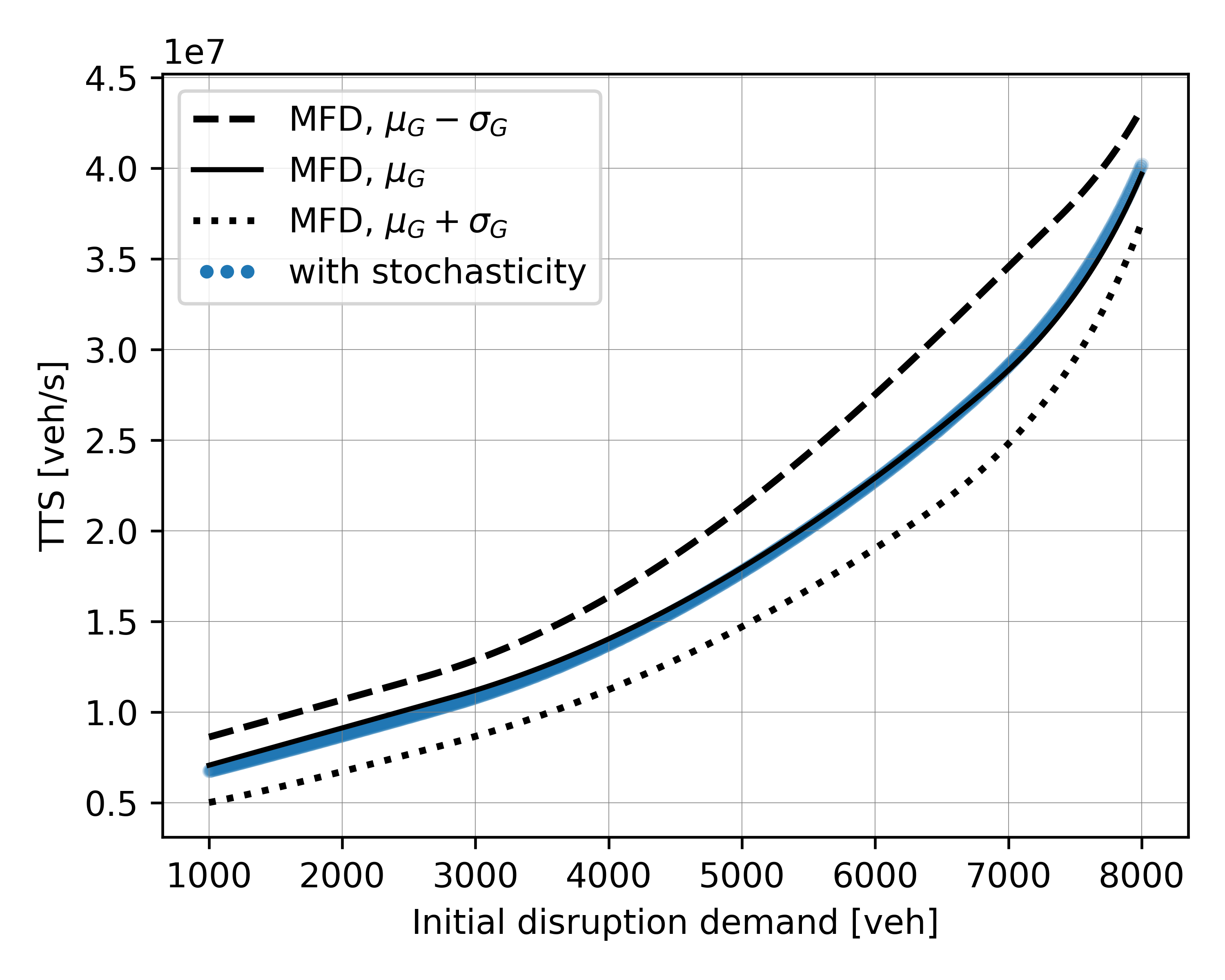
(a) Demand disruption and TTS

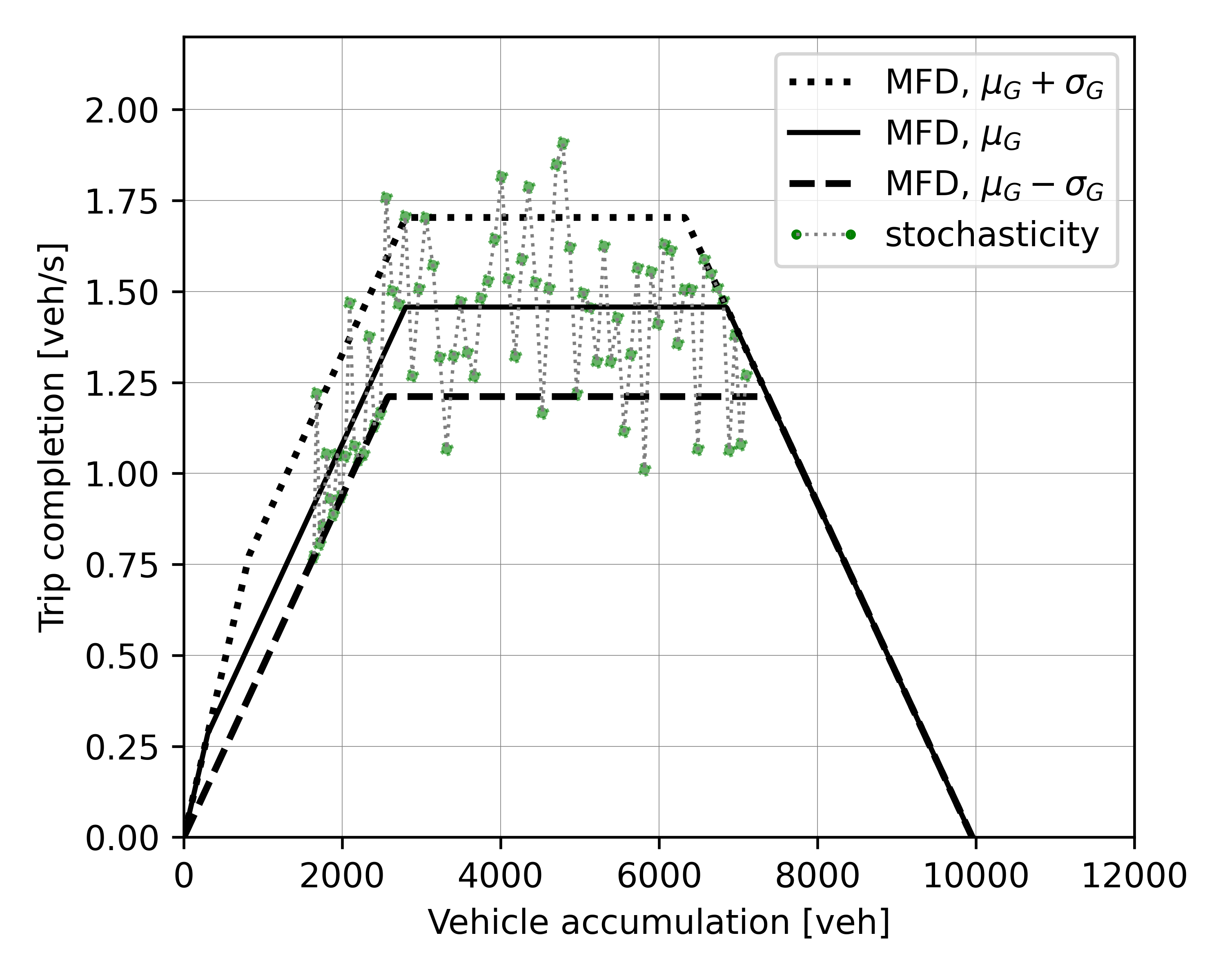
(b) Stochasticity on the MFD

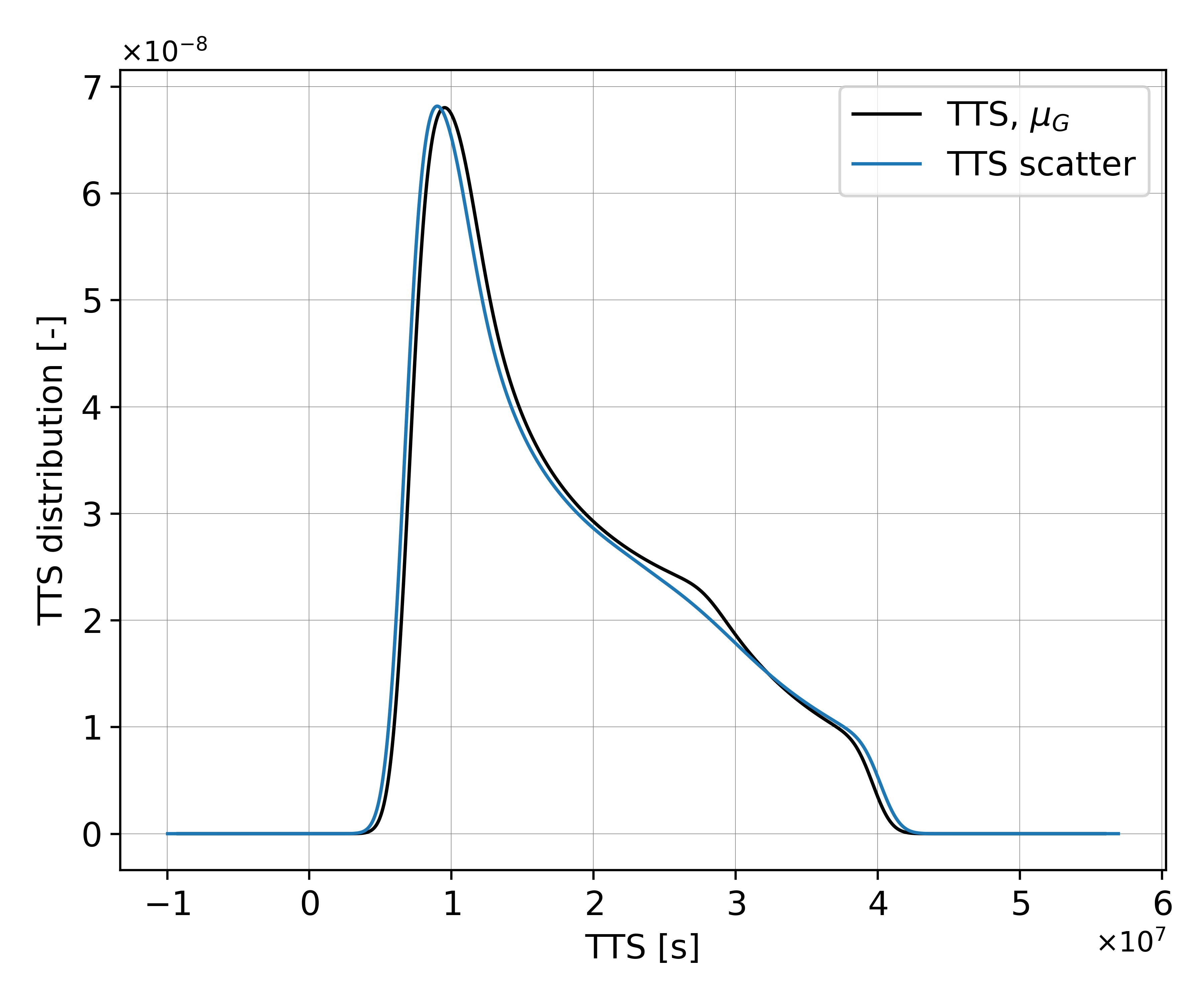
(c) TTS distribution w/wo stochasticity

Figure 10: Numerical simulation for demand disruption with stochasticity

Since the blue curve composed from the scattering points closely aligns with the solid curve, it can be inferred that the influence of realistic stochasticity on the MFD is mostly negligible. Nevertheless, an intriguing observation is that, when the disruption demand is relatively low, the blue curve dips slightly below the MFD of the solid curve. However, the blue curve appears to exceed the TTS of the well-defined MFD when the demand is substantial. This may indicate that the recovery process with stochasticity can possibly have a larger second derivative (although two linear curves share the same second derivative of zero but different slopes can yield a similar observation). When we show the distribution of these two curves, as in Fig. 10(c), the TTS with stochasticity has a more concentrated distribution at a lower value while having a marginally longer tail pointing to the right, showing a more left-skewed distribution compared to the one without realistic stochasticity. This can also be validated by calculating the skewness of these two curves. When there is no stochasticity, the skewness is 0.67 while the skewness for the blue curve has a value of 0.70. As a greater skewness indicates a more fragile system, it means by introducing realistic stochasticity, the urban road network becomes even more fragile. It makes particular sense that as per definition, a fragile system should exhibit a much more degraded performance with larger disruptions brought by stochasticity, resulting in poor adaptability to uncertainties.

Likewise, we showcase that supply disruptions can signify the fragile nature of transportation systems as well. With the same simulation environment, instead of the linearly increasing initial disruption demand, now a linearly growing supply disruption magnitude coefficient $r$ from 0 to 0.5 is considered. The simulation of the recovery process from the supply disruption along with 1000 uniformed sampled points between 0 and 0.5 is shown in Fig. 11(a). First of all, as the blue curve with stochasticity lies below the curve from the deterministic MFD with the mean green time, it means that the network with stochasticity has a better performance. This performance improvement can be attributed to the fact that, prior to reaching the maximal capacity, the upper MFD in the dotted curve generated from MoC keeps a larger space from the solid curve MFD profile compared to the distance between the lower MFD in the dashed curve. Therefore, although the likelihood of sampling a trip completion above or below the mean MFD profile is the same, there is a higher probability that the gained value of trip completion will surpass the loss caused by stochasticity. Despite this gain in system performance, when we calculate the skewness of distribution, we get a value of 0.49 for the deterministic MFD and 0.53 for the MFD when considering uncertainty, demonstrating again that stochasticity escalates the fragile response of the road transportation systems. Hence, the transportation systems have been demonstrated to be fragile with numerical simulation and such fragility has been reinforced with stochasticity in this work.

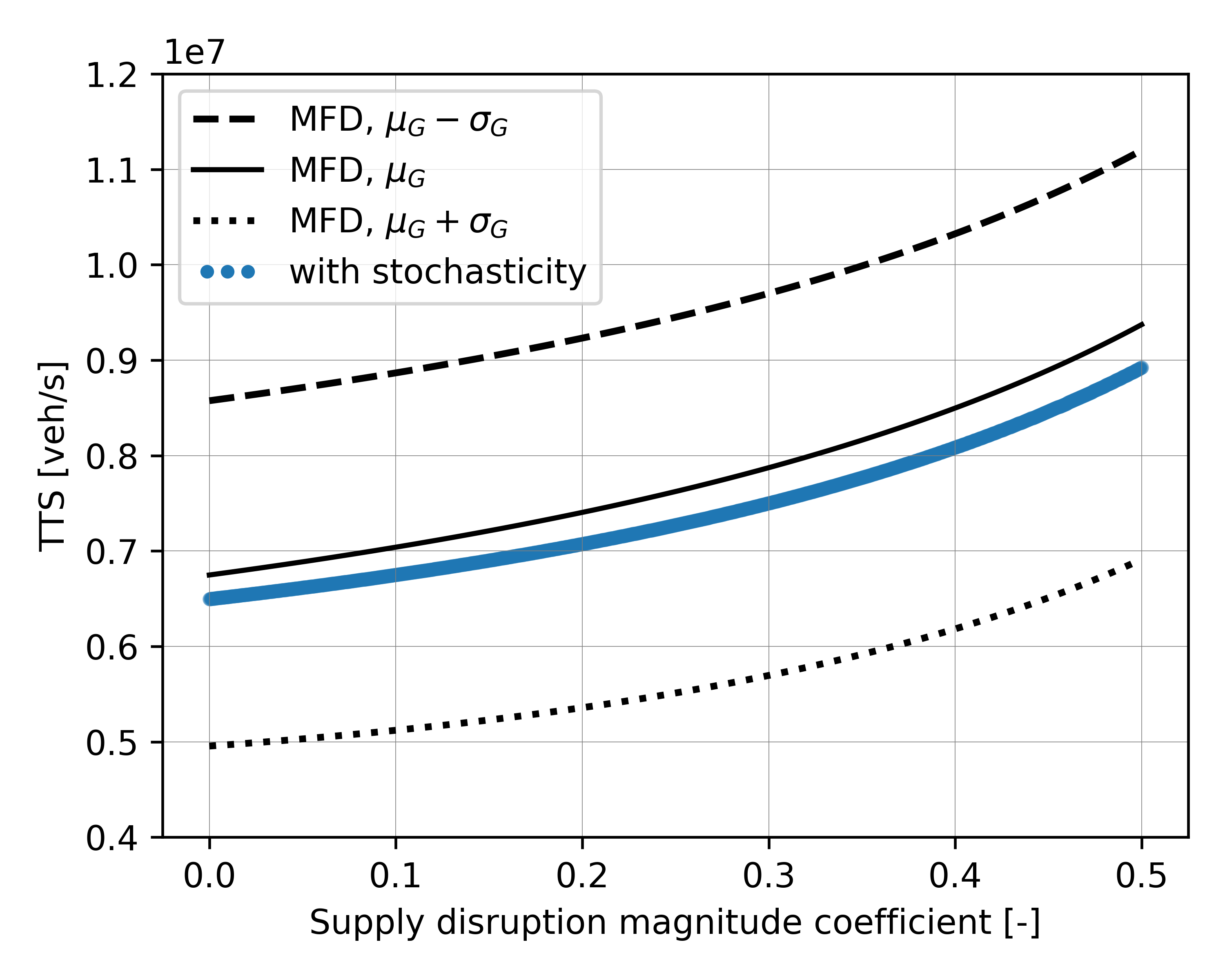
(a) Supply disruption and the TTS

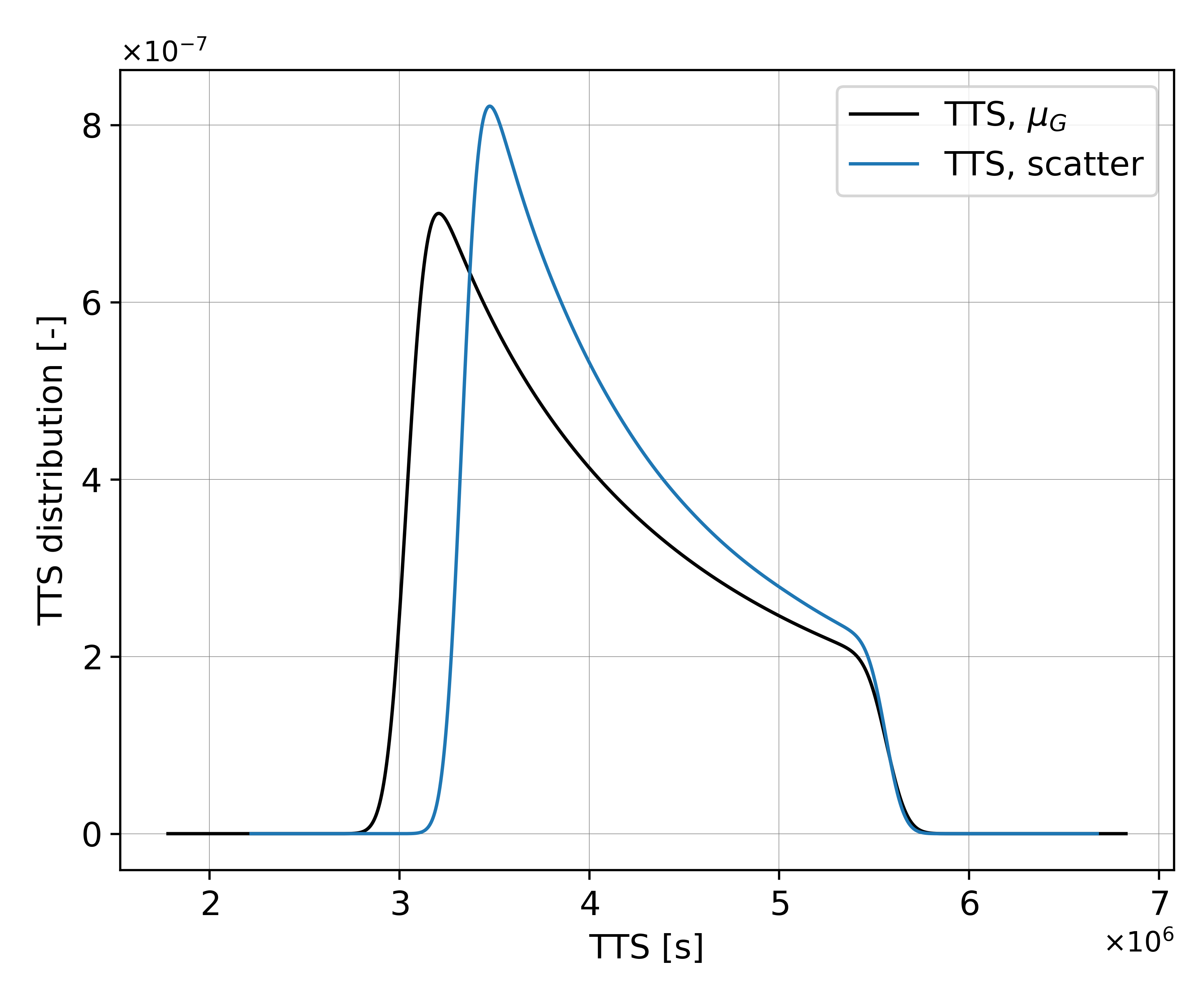
(b) TTS distribution w/wo stochasticity

Figure 11: Numerical simulation for supply disruption with stochasticity

6 Conclusion

This research systematically demonstrated the fragile nature of road transportation systems with rigorous mathematical analysis and numerical simulation under realistic stochasticity. The mathematical proof comprehends the study of fragility under 1) microscopic - macroscopic, 2) demand disruption - supply disruption, and 3) onset of disruption - recovery from disruption. With essential assumptions regarding the disruption density in comparison to the critical density as well as the base traffic demand, we have validated the fragility of road transportation systems from various perspectives. Furthermore, through a numerical simulation with realistic data, we concluded that real-world stochasticity has a limited impact on the fragile characteristics of the system but contributes to rendering the system even more fragile. As early findings have also pointed out the possibilities of applying MFDs in other transportation modes, the fragility observed in urban road networks may well be extended to various transportation systems. This study aims to offer insights to researchers, emphasizing the fragile characteristics of transportation systems and encouraging the design of antifragile traffic control strategies in the future.

7 CRediT authorship contribution statement

Linghang Sun: Conceptualization, Investigation, Methodology, Visualization, Writing – original draft. Yifan Zhang: Methodology, Visualization, Writing - review & editing. Cristian Axenie: Project administration, Resources, Writing - review & editing. Margherita Grossi: Project administration, Resources, Writing - review & editing. Anastasios Kouvelas: Supervision, Writing - review & editing. Michail A. Makridis: Conceptualization, Methodology, Supervision, Writing - review & editing.

8 Declaration of Competing Interest

This research was kindly funded by the Huawei Munich Research Center under the framework of the Antigones project, with one of our co-authors being employed at the said company. Otherwise, the authors declare that they have no known competing financial interests or personal relationships that could have appeared to influence the work reported in this paper.

References

- Ambühl et al. (2020) Ambühl, L., Loder, A., Bliemer, M.C., Menendez, M., Axhausen, K.W., 2020. A functional form with a physical meaning for the macroscopic fundamental diagram. Transportation Research Part B: Methodological 137, 119–132. URL: https://linkinghub.elsevier.com/retrieve/pii/S0191261517310123, doi:10.1016/j.trb.2018.10.013.
- Ambühl et al. (2021) Ambühl, L., Loder, A., Leclercq, L., Menendez, M., 2021. Disentangling the city traffic rhythms: A longitudinal analysis of MFD patterns over a year. Transportation Research Part C: Emerging Technologies 126, 103065. URL: https://www.sciencedirect.com/science/article/pii/S0968090X21000917, doi:10.1016/j.trc.2021.103065.
- Ampountolas et al. (2017) Ampountolas, K., Zheng, N., Geroliminis, N., 2017. Macroscopic modelling and robust control of bi-modal multi-region urban road networks. Transportation Research Part B: Methodological 104, 616–637. URL: https://www.sciencedirect.com/science/article/pii/S0191261515300370, doi:10.1016/j.trb.2017.05.007.
- Axenie et al. (2022) Axenie, C., Kurz, D., Saveriano, M., 2022. Antifragile Control Systems: The Case of an Anti-Symmetric Network Model of the Tumor-Immune-Drug Interactions. Symmetry 14, 2034. doi:10.3390/sym14102034.
- Axenie et al. (2023) Axenie, C., López-Corona, O., Makridis, M.A., Akbarzadeh, M., Saveriano, M., Stancu, A., West, J., 2023. Antifragility as a complex system’s response to perturbations, volatility, and time. URL: http://arxiv.org/abs/2312.13991, doi:10.48550/arXiv.2312.13991. arXiv:2312.13991 [q-bio].
- Axenie and Saveriano (2023) Axenie, C., Saveriano, M., 2023. Antifragile Control Systems: The case of mobile robot trajectory tracking in the presence of uncertainty.
- Büchel et al. (2022) Büchel, B., Marra, A.D., Corman, F., 2022. COVID-19 as a window of opportunity for cycling: Evidence from the first wave. Transport Policy 116, 144–156. URL: https://www.sciencedirect.com/science/article/pii/S0967070X21003565, doi:10.1016/j.tranpol.2021.12.003.
- Calvert and Snelder (2018) Calvert, S.C., Snelder, M., 2018. A methodology for road traffic resilience analysis and review of related concepts. Transportmetrica A: Transport Science 14, 130–154. URL: https://doi.org/10.1080/23249935.2017.1363315, doi:10.1080/23249935.2017.1363315. publisher: Taylor & Francis _eprint: https://doi.org/10.1080/23249935.2017.1363315.
- Cats (2016) Cats, O., 2016. The robustness value of public transport development plans. Journal of Transport Geography 51, 236–246. URL: https://www.sciencedirect.com/science/article/pii/S0966692316000120, doi:10.1016/j.jtrangeo.2016.01.011.
- Chang and Xiang (2003) Chang, G.L., Xiang, H., 2003. The relationship between congestion levels and accidents URL: https://trid.trb.org/view/680981. number: MD-03-SP 208B46,.
- Chen et al. (2022) Chen, C., Huang, Y.P., Lam, W.H.K., Pan, T.L., Hsu, S.C., Sumalee, A., Zhong, R.X., 2022. Data efficient reinforcement learning and adaptive optimal perimeter control of network traffic dynamics. Transportation Research Part C: Emerging Technologies 142, 103759. doi:10.1016/j.trc.2022.103759.
- Ciuffini et al. (2023) Ciuffini, F., Tengattini, S., Bigazzi, A.Y., 2023. Mitigating Increased Driving after the COVID-19 Pandemic: An Analysis on Mode Share, Travel Demand, and Public Transport Capacity. Transportation Research Record 2677, 154–167. URL: https://doi.org/10.1177/03611981211037884, doi:10.1177/03611981211037884. publisher: SAGE Publications Inc.
- Coppitters and Contino (2023) Coppitters, D., Contino, F., 2023. Optimizing upside variability and antifragility in renewable energy system design. Scientific Reports 13, 9138. URL: https://www.nature.com/articles/s41598-023-36379-8, doi:10.1038/s41598-023-36379-8. number: 1 Publisher: Nature Publishing Group.
- Corman et al. (2014) Corman, F., D’Ariano, A., Hansen, I.A., 2014. Evaluating Disturbance Robustness of Railway Schedules. Journal of Intelligent Transportation Systems 18, 106–120. URL: https://doi.org/10.1080/15472450.2013.801714, doi:10.1080/15472450.2013.801714. publisher: Taylor & Francis _eprint: https://doi.org/10.1080/15472450.2013.801714.
- Corman et al. (2019) Corman, F., Henken, J., Keyvan-Ekbatani, M., 2019. Macroscopic fundamental diagrams for train operations - are we there yet?, in: 2019 6th International Conference on Models and Technologies for Intelligent Transportation Systems (MT-ITS), pp. 1–8. URL: https://ieeexplore.ieee.org/abstract/document/8883374, doi:10.1109/MTITS.2019.8883374.
- Corman et al. (2018) Corman, F., Quaglietta, E., Goverde, R.M.P., 2018. Automated real-time railway traffic control: an experimental analysis of reliability, resilience and robustness. Transportation Planning and Technology 41, 421–447. URL: https://doi.org/10.1080/03081060.2018.1453916, doi:10.1080/03081060.2018.1453916. publisher: Routledge _eprint: https://doi.org/10.1080/03081060.2018.1453916.
- Daganzo (1994) Daganzo, C.F., 1994. The cell transmission model: A dynamic representation of highway traffic consistent with the hydrodynamic theory. Transportation Research Part B: Methodological 28, 269–287. URL: https://www.sciencedirect.com/science/article/pii/0191261594900027, doi:10.1016/0191-2615(94)90002-7.
- Daganzo (2005) Daganzo, C.F., 2005. A variational formulation of kinematic waves: basic theory and complex boundary conditions. Transportation Research Part B: Methodological 39, 187–196. URL: https://www.sciencedirect.com/science/article/pii/S0191261504000487, doi:10.1016/j.trb.2004.04.003.
- Daganzo and Geroliminis (2008) Daganzo, C.F., Geroliminis, N., 2008. An analytical approximation for the macroscopic fundamental diagram of urban traffic. Transportation Research Part B: Methodological 42, 771–781. URL: https://www.sciencedirect.com/science/article/pii/S0191261508000799, doi:10.1016/j.trb.2008.06.008.
- Daganzo et al. (2018) Daganzo, C.F., Lehe, L.J., Argote-Cabanero, J., 2018. Adaptive offsets for signalized streets. Transportation Research Part B: Methodological 117, 926–934. URL: https://linkinghub.elsevier.com/retrieve/pii/S0191261517306914, doi:10.1016/j.trb.2017.08.011.
- Dickerson et al. (2000) Dickerson, A., Peirson, J., Vickerman, R., 2000. Road Accidents and Traffic Flows: An Econometric Investigation. Economica 67, 101–121. URL: https://onlinelibrary.wiley.com/doi/abs/10.1111/1468-0335.00198, doi:10.1111/1468-0335.00198. _eprint: https://onlinelibrary.wiley.com/doi/pdf/10.1111/1468-0335.00198.
- Dowling and Skabardonis (1993) Dowling, R., Skabardonis, A., 1993. Improving average travel speeds estimated by planning models. Transportation Research Record , 68–68.
- Duan and Lu (2014) Duan, Y., Lu, F., 2014. Robustness of city road networks at different granularities. Physica A: Statistical Mechanics and its Applications 411, 21–34. URL: https://www.sciencedirect.com/science/article/pii/S037843711400466X, doi:10.1016/j.physa.2014.05.073.
- Federal Statistical Office of Switzerland (2020) Federal Statistical Office of Switzerland, 2020. Mobilität und Verkehr: Panorama - 2020 | Publikation. URL: https://www.bfs.admin.ch/asset/de/13695321.
- Fuchs and Corman (2019) Fuchs, F., Corman, F., 2019. An Open Toolbox for Integrated Optimization of Public Transport, in: 2019 6th International Conference on Models and Technologies for Intelligent Transportation Systems (MT-ITS), pp. 1–7. URL: https://ieeexplore.ieee.org/abstract/document/8883335, doi:10.1109/MTITS.2019.8883335.
- Genser and Kouvelas (2022) Genser, A., Kouvelas, A., 2022. Dynamic optimal congestion pricing in multi-region urban networks by application of a Multi-Layer-Neural network. Transportation Research Part C: Emerging Technologies 134, 103485. URL: https://www.sciencedirect.com/science/article/pii/S0968090X2100471X, doi:10.1016/j.trc.2021.103485.
- Genser et al. (2023) Genser, A., Makridis, M.A., Yang, K., Abmühl, L., Menendez, M., Kouvelas, A., 2023. A traffic signal and loop detector dataset of an urban intersection regulated by a fully actuated signal control system. Data in Brief 48, 109117. URL: https://www.sciencedirect.com/science/article/pii/S2352340923002366, doi:10.1016/j.dib.2023.109117.
- Genser et al. (2024) Genser, A., Makridis, M.A., Yang, K., Ambühl, L., Menendez, M., Kouvelas, A., 2024. Time-to-Green Predictions for Fully-Actuated Signal Control Systems With Supervised Learning. IEEE Transactions on Intelligent Transportation Systems , 1–14URL: https://ieeexplore.ieee.org/abstract/document/10400986, doi:10.1109/TITS.2023.3348634. conference Name: IEEE Transactions on Intelligent Transportation Systems.
- Geroliminis and Daganzo (2008) Geroliminis, N., Daganzo, C.F., 2008. Existence of urban-scale macroscopic fundamental diagrams: Some experimental findings. Transportation Research Part B: Methodological 42, 759–770. URL: https://www.sciencedirect.com/science/article/pii/S0191261508000180, doi:10.1016/j.trb.2008.02.002.
- Geroliminis et al. (2013) Geroliminis, N., Haddad, J., Ramezani, M., 2013. Optimal Perimeter Control for Two Urban Regions With Macroscopic Fundamental Diagrams: A Model Predictive Approach. IEEE Transactions on Intelligent Transportation Systems 14, 348–359. doi:10.1109/TITS.2012.2216877. conference Name: IEEE Transactions on Intelligent Transportation Systems.
- Gibson et al. (2002) Gibson, S., Cooper, G., Ball, B., 2002. Developments in Transport Policy: The Evolution of Capacity Charges on the UK Rail Network. Journal of Transport Economics and Policy (JTEP) 36, 341–354.
- Greenshields et al. (1934) Greenshields, B.D., Thompson, J.T., Dickinson, H.C., Swinton, R.S., 1934. The photographic method of studying traffic behavior. Highway Research Board Proceedings 13. URL: https://trid.trb.org/view/120821.
- Haddad and Mirkin (2017) Haddad, J., Mirkin, B., 2017. Coordinated distributed adaptive perimeter control for large-scale urban road networks. Transportation Research Part C: Emerging Technologies 77, 495–515. URL: https://www.sciencedirect.com/science/article/pii/S0968090X16302509, doi:10.1016/j.trc.2016.12.002.
- Haddad and Shraiber (2014) Haddad, J., Shraiber, A., 2014. Robust perimeter control design for an urban region. Transportation Research Part B: Methodological 68, 315–332. URL: https://www.sciencedirect.com/science/article/pii/S0191261514001179, doi:10.1016/j.trb.2014.06.010.
- (35) Isaacson, D., Robinson, J., Swenson, H., Denery, D., . A Concept for Robust, High Density Terminal Air Traffic Operations, in: 10th AIAA Aviation Technology, Integration, and Operations (ATIO) Conference. American Institute of Aeronautics and Astronautics. URL: https://arc.aiaa.org/doi/abs/10.2514/6.2010-9292, doi:10.2514/6.2010-9292. _eprint: https://arc.aiaa.org/doi/pdf/10.2514/6.2010-9292.
- Jensen (1906) Jensen, J.L.W.V., 1906. Sur les fonctions convexes et les inégualités entre les valeurs Moyennes URL: https://zenodo.org/records/2371297, doi:10.1007/bf02418571.
- Kim et al. (2020) Kim, H., Muñoz, S., Osuna, P., Gershenson, C., 2020. Antifragility Predicts the Robustness and Evolvability of Biological Networks through Multi-Class Classification with a Convolutional Neural Network. Entropy 22, 986. doi:10.3390/e22090986.
- Kouvelas et al. (2017) Kouvelas, A., Saeedmanesh, M., Geroliminis, N., 2017. Enhancing model-based feedback perimeter control with data-driven online adaptive optimization. Transportation Research Part B: Methodological 96, 26–45. URL: https://www.sciencedirect.com/science/article/pii/S019126151630710X, doi:10.1016/j.trb.2016.10.011.
- Larsen et al. (2014) Larsen, R., Pranzo, M., D’Ariano, A., Corman, F., Pacciarelli, D., 2014. Susceptibility of optimal train schedules to stochastic disturbances of process times. Flexible Services and Manufacturing Journal 26, 466–489. URL: https://doi.org/10.1007/s10696-013-9172-9, doi:10.1007/s10696-013-9172-9.
- Laval and Castrillón (2015) Laval, J.A., Castrillón, F., 2015. Stochastic approximations for the macroscopic fundamental diagram of urban networks. Transportation Research Part B: Methodological 81, 904–916. URL: https://www.sciencedirect.com/science/article/pii/S0191261515001964, doi:10.1016/j.trb.2015.09.002.
- Leclercq and Geroliminis (2013) Leclercq, L., Geroliminis, N., 2013. Estimating MFDs in simple networks with route choice. Transportation Research Part B: Methodological 57, 468–484. URL: https://linkinghub.elsevier.com/retrieve/pii/S0191261513000878, doi:10.1016/j.trb.2013.05.005.
- Leclercq et al. (2021) Leclercq, L., Ladino, A., Becarie, C., 2021. Enforcing optimal routing through dynamic avoidance maps. Transportation Research Part B: Methodological 149, 118–137. URL: https://www.sciencedirect.com/science/article/pii/S0191261521000813, doi:10.1016/j.trb.2021.05.002.
- Lo et al. (2006) Lo, H.K., Luo, X.W., Siu, B.W.Y., 2006. Degradable transport network: Travel time budget of travelers with heterogeneous risk aversion. Transportation Research Part B: Methodological 40, 792–806. URL: https://www.sciencedirect.com/science/article/pii/S0191261505001177, doi:10.1016/j.trb.2005.10.003.
- Manso et al. (2020) Manso, G., Balsmeier, B., Fleming, L., 2020. Heterogeneous Innovation and the Antifragile Economy .
- Mariotte et al. (2017) Mariotte, G., Leclercq, L., Laval, J.A., 2017. Macroscopic urban dynamics: Analytical and numerical comparisons of existing models. Transportation Research Part B: Methodological 101, 245–267. URL: https://www.sciencedirect.com/science/article/pii/S0191261516307846, doi:10.1016/j.trb.2017.04.002.
- Marra et al. (2022) Marra, A.D., Sun, L., Corman, F., 2022. The impact of COVID-19 pandemic on public transport usage and route choice: Evidences from a long-term tracking study in urban area. Transport Policy 116, 258–268. URL: https://www.sciencedirect.com/science/article/pii/S0967070X21003620, doi:10.1016/j.tranpol.2021.12.009.
- Mattsson and Jenelius (2015) Mattsson, L.G., Jenelius, E., 2015. Vulnerability and resilience of transport systems – A discussion of recent research. Transportation Research Part A: Policy and Practice 81, 16–34. URL: https://www.sciencedirect.com/science/article/pii/S0965856415001603, doi:10.1016/j.tra.2015.06.002.
- Ng and Waller (2010) Ng, M., Waller, S.T., 2010. A computationally efficient methodology to characterize travel time reliability using the fast Fourier transform. Transportation Research Part B: Methodological 44, 1202–1219. URL: https://www.sciencedirect.com/science/article/pii/S0191261510000238, doi:10.1016/j.trb.2010.02.008.
- Qu et al. (2017) Qu, X., Zhang, J., Wang, S., 2017. On the stochastic fundamental diagram for freeway traffic: Model development, analytical properties, validation, and extensive applications. Transportation Research Part B: Methodological 104, 256–271. URL: https://www.sciencedirect.com/science/article/pii/S0191261516306622, doi:10.1016/j.trb.2017.07.003.
- Rodrigues and Azevedo (2019) Rodrigues, F., Azevedo, C.L., 2019. Towards Robust Deep Reinforcement Learning for Traffic Signal Control: Demand Surges, Incidents and Sensor Failures, in: 2019 IEEE Intelligent Transportation Systems Conference (ITSC), pp. 3559–3566. doi:10.1109/ITSC.2019.8917451.
- Ruel et al. (1999) Ruel, J.J., Ayres, M.P., Ruel, J.J., Ayres, M.P., 1999. Jensen’s inequality predicts effects of environmental variation. Trends in Ecology & Evolution 14, 361–366. URL: https://www.cell.com/trends/ecology-evolution/abstract/S0169-5347(99)01664-X, doi:10.1016/S0169-5347(99)01664-X. publisher: Elsevier.
- Safadi et al. (2023) Safadi, Y., Fu, R., Quan, Q., Haddad, J., 2023. Macroscopic Fundamental Diagrams for Low-Altitude Air city Transport. Transportation Research Part C: Emerging Technologies 152, 104141. URL: https://www.sciencedirect.com/science/article/pii/S0968090X23001304, doi:10.1016/j.trc.2023.104141.
- Saffari et al. (2022) Saffari, E., Yildirimoglu, M., Hickman, M., 2022. Data fusion for estimating Macroscopic Fundamental Diagram in large-scale urban networks. Transportation Research Part C: Emerging Technologies 137, 103555. URL: https://www.sciencedirect.com/science/article/pii/S0968090X22000043, doi:10.1016/j.trc.2022.103555.
- Saidi et al. (2023) Saidi, S., Koutsopoulos, H.N., Wilson, N.H.M., Zhao, J., 2023. Train following model for urban rail transit performance analysis. Transportation Research Part C: Emerging Technologies 148, 104037. URL: https://www.sciencedirect.com/science/article/pii/S0968090X23000268, doi:10.1016/j.trc.2023.104037.
- Schüssler and Axhausen (2008) Schüssler, N., Axhausen, K.W., 2008. Identifying trips and activities and their characteristics from gps raw data without further information. Arbeitsberichte Verkehrs-und Raumplanung 502.
- Shang et al. (2022) Shang, W.L., Gao, Z., Daina, N., Zhang, H., Long, Y., Guo, Z., Ochieng, W.Y., 2022. Benchmark Analysis for Robustness of Multi-Scale Urban Road Networks Under Global Disruptions. IEEE Transactions on Intelligent Transportation Systems , 1–11URL: https://ieeexplore.ieee.org/abstract/document/9714769, doi:10.1109/TITS.2022.3149969. conference Name: IEEE Transactions on Intelligent Transportation Systems.
- Siqueira et al. (2016) Siqueira, A.F., Peixoto, C.J.T., Wu, C., Qian, W.L., 2016. Effect of stochastic transition in the fundamental diagram of traffic flow. Transportation Research Part B: Methodological 87, 1–13. URL: https://www.sciencedirect.com/science/article/pii/S019126151600028X, doi:10.1016/j.trb.2016.02.003.
- Sirmatel and Geroliminis (2018) Sirmatel, I.I., Geroliminis, N., 2018. Economic Model Predictive Control of Large-Scale Urban Road Networks via Perimeter Control and Regional Route Guidance. IEEE Transactions on Intelligent Transportation Systems 19, 1112–1121. URL: https://ieeexplore.ieee.org/abstract/document/7964750, doi:10.1109/TITS.2017.2716541. conference Name: IEEE Transactions on Intelligent Transportation Systems.
- Skabardonis and Dowling (1997) Skabardonis, A., Dowling, R., 1997. Improved speed-flow relationships for planning applications. Transportation research record 1572, 18–23.
- Sun et al. (2024) Sun, L., Makridis, M.A., Genser, A., Axenie, C., Grossi, M., Kouvelas, A., 2024. Antifragile Perimeter Control: Anticipating and Gaining from Disruptions with Reinforcement Learning. URL: https://arxiv.org/abs/2402.12665v1.
- Taleb (2012) Taleb, N.N., 2012. Antifragile: Things That Gain from Disorder. Reprint edition ed., Random House Publishing Group, New York.
- Taleb and Douady (2013) Taleb, N.N., Douady, R., 2013. Mathematical definition, mapping, and detection of (anti)fragility. Quantitative Finance 13, 1677–1689. doi:10.1080/14697688.2013.800219.
- Taleb and West (2023) Taleb, N.N., West, J., 2023. Working with Convex Responses: Antifragility from Finance to Oncology. Entropy 25, 343. URL: https://www.mdpi.com/1099-4300/25/2/343, doi:10.3390/e25020343. number: 2 Publisher: Multidisciplinary Digital Publishing Institute.
- Tang et al. (2020) Tang, J., Heinimann, H., Han, K., Luo, H., Zhong, B., 2020. Evaluating resilience in urban transportation systems for sustainability: A systems-based Bayesian network model. Transportation Research Part C: Emerging Technologies 121, 102840. URL: https://www.sciencedirect.com/science/article/pii/S0968090X20307427, doi:10.1016/j.trc.2020.102840.
- Tilg et al. (2020) Tilg, G., Amini, S., Busch, F., 2020. Evaluation of analytical approximation methods for the macroscopic fundamental diagram. Transportation Research Part C: Emerging Technologies 114, 1–19. URL: https://www.sciencedirect.com/science/article/pii/S0968090X19307661, doi:10.1016/j.trc.2020.02.003.
- U.S. Bureau of Public Roads (1964) U.S. Bureau of Public Roads, 1964. Traffic assignment manual for application with a large, high speed computer. US Department of Commerce.
- U.S. Congress, Office of Technology Assessment (1984) U.S. Congress, Office of Technology Assessment, 1984. Airport system development. U.S. Government Printing Office. Google-Books-ID: hihBG2mzB1MC.
- U.S. Department of Transportation (2019) U.S. Department of Transportation, 2019. National Transportation Statistics (NTS). URL: https://tinyurl.com/rosapntlbtsNTS, doi:10.21949/1503663. publisher: Not Available.
- Wang et al. (2014) Wang, J.Y.T., Ehrgott, M., Chen, A., 2014. A bi-objective user equilibrium model of travel time reliability in a road network. Transportation Research Part B: Methodological 66, 4–15. URL: https://www.sciencedirect.com/science/article/pii/S019126151300180X, doi:10.1016/j.trb.2013.10.007.
- Yang et al. (2019) Yang, K., Menendez, M., Zheng, N., 2019. Heterogeneity aware urban traffic control in a connected vehicle environment: A joint framework for congestion pricing and perimeter control. Transportation Research Part C: Emerging Technologies 105, 439–455. URL: https://www.sciencedirect.com/science/article/pii/S0968090X18316127, doi:10.1016/j.trc.2019.06.007.
- Zehe et al. (2015) Zehe, D., Grotzky, D., Aydt, H., Cai, W., Knoll, A., 2015. Traffic Simulation Performance Optimization through Multi-Resolution Modeling of Road Segments, in: Proceedings of the 3rd ACM SIGSIM Conference on Principles of Advanced Discrete Simulation, Association for Computing Machinery, New York, NY, USA. pp. 281–288. URL: https://dl.acm.org/doi/10.1145/2769458.2769475, doi:10.1145/2769458.2769475.
- Zhang and Zhang (2021) Zhang, R., Zhang, J., 2021. Long-term pathways to deep decarbonization of the transport sector in the post-COVID world. Transport Policy 110, 28–36. URL: https://www.sciencedirect.com/science/article/pii/S0967070X21001621, doi:10.1016/j.tranpol.2021.05.018.
- Zhou and Gayah (2021) Zhou, D., Gayah, V.V., 2021. Model-free perimeter metering control for two-region urban networks using deep reinforcement learning. Transportation Research Part C: Emerging Technologies 124, 102949. URL: https://linkinghub.elsevier.com/retrieve/pii/S0968090X20308469, doi:10.1016/j.trc.2020.102949.
- Zhou and Gayah (2023) Zhou, D., Gayah, V.V., 2023. Scalable multi-region perimeter metering control for urban networks: A multi-agent deep reinforcement learning approach. Transportation Research Part C: Emerging Technologies 148, 104033. URL: https://linkinghub.elsevier.com/retrieve/pii/S0968090X23000220, doi:10.1016/j.trc.2023.104033.
- Zhou et al. (2019) Zhou, Y., Wang, J., Yang, H., 2019. Resilience of Transportation Systems: Concepts and Comprehensive Review. IEEE Transactions on Intelligent Transportation Systems 20, 4262–4276. doi:10.1109/TITS.2018.2883766. conference Name: IEEE Transactions on Intelligent Transportation Systems.