Can we Constrain Concept Bottleneck Models to
Learn Semantically Meaningful Input Features?
Abstract
Concept Bottleneck Models (CBMs) are considered inherently interpretable because they first predict a set of human-defined concepts before using these concepts to predict the output of a downstream task. For inherent interpretability to be fully realised, and ensure trust in a model’s output, we need to guarantee concepts are predicted based on semantically mapped input features. For example, one might expect the pixels representing a broken bone in an image to be used for the prediction of a fracture. However, current literature indicates this is not the case, as concept predictions are often mapped to irrelevant input features. We hypothesise that this occurs when concept annotations are inaccurate or how input features should relate to concepts is unclear. In general, the effect of dataset labelling on concept representations in CBMs remains an understudied area. Therefore, in this paper, we examine how CBMs learn concepts from datasets with fine-grained concept annotations. We demonstrate that CBMs can learn concept representations with semantic mapping to input features by removing problematic concept correlations, such as two concepts always appearing together. To support our evaluation, we introduce a new synthetic image dataset based on a playing cards domain, which we hope will serve as a benchmark for future CBM research. For validation, we provide empirical evidence on a real-world dataset of chest X-rays, to demonstrate semantically meaningful concepts can be learned in real-world applications.
1 Introduction
Concept Bottleneck Models (CBMs) Koh et al. (2020) have been positioned as improving human collaboration as they are inherently interpretable Koh et al. (2020). This capability is enabled by the model predicting a vector of human-defined concepts and a downstream task. Concept predictions can be inspected and modified to reveal the reasoning the model made for a downstream task prediction. However, this may be misleading to humans interpreting the machine’s outputs if the model does not predict concepts based on their expected input features, but the human assumes it does. For humans to make full use of a model they will need to trust the model’s output but a lack of understanding of the causes for a decision will instead result in a loss of trust Miller (2019). To benefit the most from CBM’s capabilities, they will need to be trained so input features map to concepts that align semantically.
During training both the concepts and downstream task are supervised with the model split into two parts, the input to the concept vector, the model part, and the concept vector to the downstream task, the model part. Splitting the model enables a human to intervene in the concept predictions by modifying them and passing them back through the model part Koh et al. (2020). Let’s say we have a model diagnosing patients from X-ray images using concepts such as “fracture” or “edema”, a radiologist can add or remove concepts from the model outputs which may result in a vastly different downstream task output and thus may influence their overall decision-making. As CBMs do not reveal the input image features used for concept predictions, the radiologist’s decision, made in collaboration with the model, may assume the model is making use of the same features they used, potentially resulting in a diagnosis missing overlooked features or including irrelevant ones.
Semantically meaningful concept mapping is when concepts are predicted based on input features with the same meaning. For instance, if a CBM predicted the concept “fracture” we may expect the pixels representing the bone and break to be the primary input features used if the model has learned a Semantically meaningful concept mapping, and is not generally distributed over the entire subject in the input image. Current literature indicates CBMs do not map input features to concepts semantically Furby et al. (2023); Margeloiu et al. (2021). The authors use saliency maps produced with model-specific techniques, such as Integrated gradients (IG) Sundararajan et al. (2017) or Layer-wise Relevance Propagation (LRP) Bach et al. (2015), to visualise the relevance of input features. It is thought that CBMs are taking shortcuts Furby et al. (2023) or encoding other information in the concept vector Marconato et al. (2022); Espinosa Zarlenga et al. (2023). It is possible, however, that this could be caused by CBMs being trained on inaccurate or weakly defined concept annotations. A popular dataset for CBM research is a modified version of Caltech-UCSD Birds-200-2011 (CUB) Wah et al. (2011) with class-level concepts Koh et al. (2020), where each sample in a class has the same set of concepts. Most concepts for CUB represent parts of a bird, however, if the image is cropped, or the bird changes appearance with gender or age, concepts may no longer match the visual appearance in the image. As CBMs are only trained on task and concept labels they have no ground truth as to what features they should use from dataset samples and instead are left to discover this. If concepts are not carefully considered when designing a dataset then there could be concepts that always appear together, potentially causing unintentional concept correlations, concepts that only appear for one downstream task, opening a shortcut the model may use for downstream task prediction, or concepts that do not have a visual representation in the input. We hypothesise that using a dataset with accurate and well-defined concepts, a CBM can learn concept representations with semantic mappings from input features. To the best of our knowledge, the dataset has had little consideration for how it affects concept representations with the only research into semantic concept mapping using the previously mentioned CUB dataset Furby et al. (2023); Margeloiu et al. (2021).
This paper presents a comprehensive analysis of the concept representations CBMs learn with various dataset configurations. We focus on training CBMs on images containing visual features that represent concepts. Our datasets include a synthetic image dataset, which enables us to explore a best-case scenario, and a chest X-ray image dataset, which demonstrates a real-world use case. Our contributions are threefold; (1) In contrast to previous studies, we demonstrate the ability of CBMs to learn concept representations that hold semantic mapping to the input space. This was shown by (2) introducing a new synthetic image dataset with fine-grained concept annotations. (3) We performed an in-depth analysis of CBMs and concluded that two factors are critical for CBMs to learn semantically meaningful input features: (i) accuracy of concept annotations and (ii) high variability in the combinations of concepts co-occurring.
2 Related Work
Previous work has explored the mappings CBMs learn Furby et al. (2023); Margeloiu et al. (2021). These show that CBMs fail to map concept outputs to semantically meaningful areas in the input image, however, they only focus on class-level concepts with the dataset CUB. This dataset has concept annotations representing visual attributes of birds but, birds can look different when they are young and old or male and female, and some concepts may be hidden from view. This was highlighted by Furby et al. (2023) and could explain the inability of CBMs to learn a semantically meaningful mapping to input features. To the best of our knowledge, there is no prior work which looks at the attribution of relevance to the input features that contribute to a model’s output(s) with CBMs trained on datasets with instance-level concepts, where each sample in a dataset has its own concept vector Koh et al. (2020), or datasets with accurate concept annotations and where the correlation between concepts has been carefully considered. Instance-level concept annotations avoid the inaccurate concept annotations seen with CUB as concepts can be fine-grained, only setting concepts to present when their visual representations can be identified in the input. We cannot jump to the conclusion that instance-level concepts are all you need. The original CUB dataset Wah et al. (2011) has instance-level concepts, but these were noisy Koh et al. (2020) which may restrict the model learning semantically meaningful concept mappings.
Other metrics to analyse the concepts CBMs learn fall under the term concept leakage Mahinpei et al. (2021), and originate from disentanglement metrics Bengio et al. (2013), where it’s generally desired for concepts to only encode information than is required to predict themselves. Mahinpei et al. (2021) evaluates whether concepts excluded from training can be predicted better than a random guess, while Marconato et al. (2022) trains models on fixed data ranges and tests whether concepts can be predicted outside of these constraints. Espinosa Zarlenga et al. (2023) introduces Oracle and Niche scores to measure concept purity. These scores measure inter-concept predictability w.r.t. the expected predictive performance of the dataset. Concept purity is argued to be better suited to CBMs than existing disentanglement metrics.
We position our work for smaller and specialised tasks Oikarinen et al. (2023) due to the complexity of creating large-scale datasets with concept annotations Kazhdan et al. (2021). Moving beyond this, recent developments with Large Language Models Oikarinen et al. (2023); Yang et al. (2023) and language-vision model, CLIP Radford et al. (2021), have the potential to automate the annotation process. Large Language Models are used to generate potential concepts and CLIP discards concepts not relevant to the input image. For now, however, we cannot guarantee all generated concepts relate to semantically meaningful input features in the input image. This can be observed in Oikarinen et al. (2023) with the concept “junk” for an image of a car or “long tail with white stripes” for an image of a bird where the tail is obscured in the image.
3 Concept Bottleneck Models
A CBM takes an input, in our case an image, which is passed through the model part, predicting a vector of concepts. Concept predictions are then passed through the model part to predict a downstream task. Concept predictions are in the range of 0 to 1 where 0 means the model is confident the concept is not present and a prediction of 1 means the model is confident the concept is present. Predictions of 0.5 and above are counted as present. A CBM prediction can be intervened by adjusting the concept outputs with new values within the range 0 and 1 and then performing the forward pass with the new set of concepts and the model part to get a new downstream task prediction.
CBMs are trained by supervising both the concepts and the downstream task given the training set where we are provided with a set of inputs , corresponding targets and vectors of concepts . A CBM in the form uses two functions: to map an input to the concept space, and to map concepts to the downstream task output. This is such that the downstream task prediction is made using only the predicted concepts.
There are three methods we can train a CBM; the independent method where each model part is trained separately and then joined together after training, the sequential method where the model parts are trained one after another, or the joint methods where the model parts are trained together.
In this paper we also train CBMs with training sets and and thus can train the model part for function on a separate dataset to the model part for function . The only limitation this causes is we are unable to train models using the joint method. This should not be a concern as the training method does not appear to make a difference to model accuracy Marconato et al. (2022).
4 Experiment Set-up
We address if CBMs can learn to map semantically meaningful input features to concepts and the effect inter-concept predictability of a dataset has on learned concept representations. For each of our experiments, we have the following dataset and model set-up.
| input | |||
| Jack of Spades | Three of Spades |
Six of
Diamonds |
|
|
Independent and
|
|||
| 0.999 | 1.0 | 0.99999 | |
|
Independent and
|
|||
| 0.99776 | 1.0 | 1.0 | |
|
Joint - Poker cards |
|||
| 0.45868 | 1.0 | 0.99996 | |
|
Standard NN |
|||
| 0.46188 | 0.74552 | 0.97131 |
4.1 Datasets
We train our models on two datasets: Playing cards, a new synthetic image dataset to evaluate CBMs with perfect concept annotations, and CheXpert, a real-world X-ray image dataset.
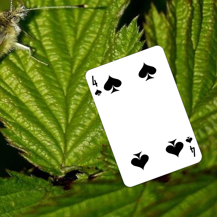
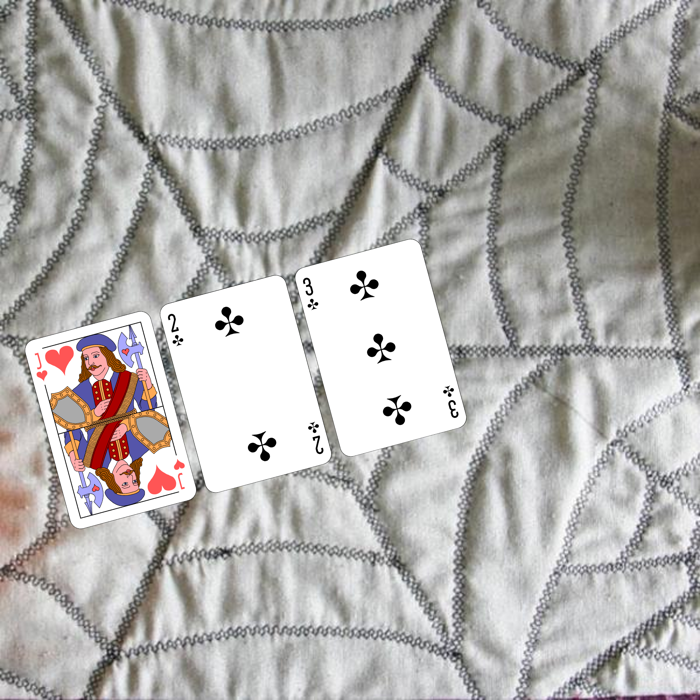
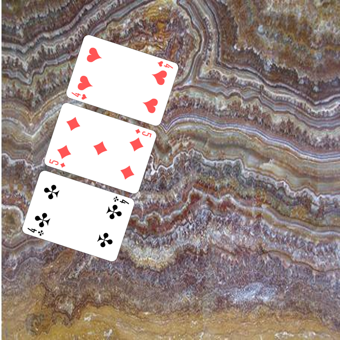
Playing cards: Playing cards is a synthetic image dataset we’re introducing to analyse CBMs free of noise and with control over how clear input features map to concept labels. Playing cards is comprised of 40,000 images in four variations: (1) single playing card, (2) three random playing cards, referred to as random cards, (3) three playing cards with a downstream task of classifying hand ranks in the game Three Card Poker, referred to as poker cards, a smaller and faster-paced version of the card game Poker, and (4) a version of poker cards with a reduced set of concepts, referred to as class-level poker cards. Each variation has a 70%-30% split between training and validation images. Both random cards and poker cards have instance-level concepts where the concepts represent the playing cards present in the input images. Class-level poker cards use class-level concepts with 11 concepts instead of the full 52 from random and poker cards. In all cases, if a concept is annotated as present, then it is visible in the corresponding image. The dataset is available for download111Playing cards dataset: Available for camera-ready submission.
CheXpert Irvin et al. (2019): We use CheXpert as an example of a real-world image dataset with visually represented concepts. We use 13 signs for the concepts with the attribute “no_findings” as the downstream task. CheXpert has instance-level concepts. The dataset contains 224,316 chest X-ray images that were scaled to 512 x 512 pixels. We use the official dataset splits from Irvin et al. (2019). For validating the model we only use frontal-view images, 202 in total. The dataset was configured with U-ones annotations which set any missing values to 0 and any uncertain annotations to 1. We also modify CheXpert to use class-level concepts with the most common concept vector for three, four and five concepts present. We refer to the original version of CheXpert as instance-level CheXpert and the class-level modifications as class-level CheXpert.
4.2 Models
The playing cards models use a VGG-11 architecture with batch normalisation Simonyan and Zisserman (2015) for the model part. For the model part, we use two linear layers with a ReLU activation function. Between the two model parts, we use a sigmoid function as this increases the independence of concept representations than the logits alternative Espinosa Zarlenga et al. (2023). We evaluate these models w.r.t. the combined concept and downstream task loss. Our random cards models achieve an average concept accuracy of 99.932%, poker card models have an average concept accuracy of 99.914% and class-level poker cards have an average concept accuracy of 99.99%. To compare CBM with a standard Neural Network (NN) we also trained models on poker cards but without concept loss, achieving an average concept accuracy of 50.25%.
Our CheXpert models use a Densenet121 architecture Huang et al. (2017) for the model part and pre-trained weights from ImageNet and two linear layers with a ReLU activation function for the model part. We evaluate this model w.r.t. Area Under the receiver operating characteristic Curve (AUC), following previous work Ye et al. (2020); Chauhan et al. (2023). Our instance-level CheXpert models achieve an average concept accuracy of 76.82% while class-level CheXpert models archived an average concept accuracy of 57.127%, 61.418% and 60.962% for the dataset version with three, four and five concepts present respectively.
Full details on model training and performance for playing card models and CheXpert models can be found in the Appendix A.1.
5 Experiments and Results
In this section, we analyse our models using both qualitative and quantitative metrics. Where relevant we have provided additional samples in the Appendix B.
5.1 Input Feature Importance
| input | Four of Clubs |
Four of
Diamonds |
Four of Spades |
| 1.0 | 1.0 | 1.0 |
| input |
Five of
Diamonds |
Five of Clubs | Ten of Hearts |
| 1.0 | 1.0 | 0.99999 |
We first evaluate feature importance using saliency mapping techniques with the playing card models. We use model-specific methods which utilise the model architecture to produce explanations by propagating a gradient backwards through the model Bach et al. (2015); Sundararajan et al. (2017); Selvaraju et al. (2017). Each of the explanation techniques produces saliency maps where we display positive relevance in red and negative relevance in blue. Saliency maps are local explanations which means any explanation only relates to a single sample and model. We are therefore limited to using these to highlight biases in the model Ribeiro et al. (2016) or otherwise provide a qualitative evaluation of feature importance.
| Cardiomegaly | Edema | Consolidation | Atelectasis | Pleural Effusion |
| 0.86032 | 0.87769 | 0.58557 | 0.44807 | 0.48908 |
| Cardiomegaly | Edema | Consolidation | Atelectasis | Pleural Effusion |
| 0.96086 | 0.85462 | 0.674 | 0.50234 | 0.62307 |
We use the technique LRP to explain the playing card models with the rules Bach et al. (2015) LRP-, where and , for the first four convolutional layers of the model from the input, LRP- for the next four convolutional layers and LRP-0 for the top three linear layers. These rules were selected to be similar to those used by Montavon et al. (2019).
|
Lung
Opacity |
Pleural Effusion |
Support
Devices |
| 0.93549 | 0.93572 | 0.93711 |
| Edema | Pleural Effusion |
Support
Devices |
| 0.96657 | 0.96679 | 0.96812 |
| Consolidation | Pleural Effusion |
Support
Devices |
| 0.98525 | 0.98471 | 0.98520 |
Figure 1 shows for random and poker card CBMs the most positively salient input features are symbols on the playing cards. Positive salience is primarily contained to the corresponding playing card for each concept with negative relevance distributed over the other playing cards. As we do not specify which input features the model should use for each concept, and we can see the models have selected features within semantically meaningful playing cards, we consider these reasonable input features for the model to use. Our standard NN was unable to localise relevance to the semantically meaningful playing cards and instead distributed it over all three cards present. In Figure 2 we show saliency maps for models trained with class-level poker cards. Despite class-level concepts being used by Furby et al. (2023); Margeloiu et al. (2021), using our dataset we successfully trained our models to recognise concepts with a semantic mapping from input features to concepts. However, this is limited to just a few concepts (see Four of Clubs and Four of Spades in Figure 2(a)). In total, only 3 concepts consistently have positive relevance applied to them by the model. This was to be expected as for some concepts there is more ambiguity regarding which input features the model should use. Class-level poker cards was designed so some concepts have a clear input feature to concept mapping such as in Figure 2(a), the concepts used for the downstream task class Three of a kind are also used by other downstream classes, while others do not, such as in Figure 2(b), Five of Clubs is only used for the downstream task class Pair. Other concepts are confined to appearing in pairs or threes.
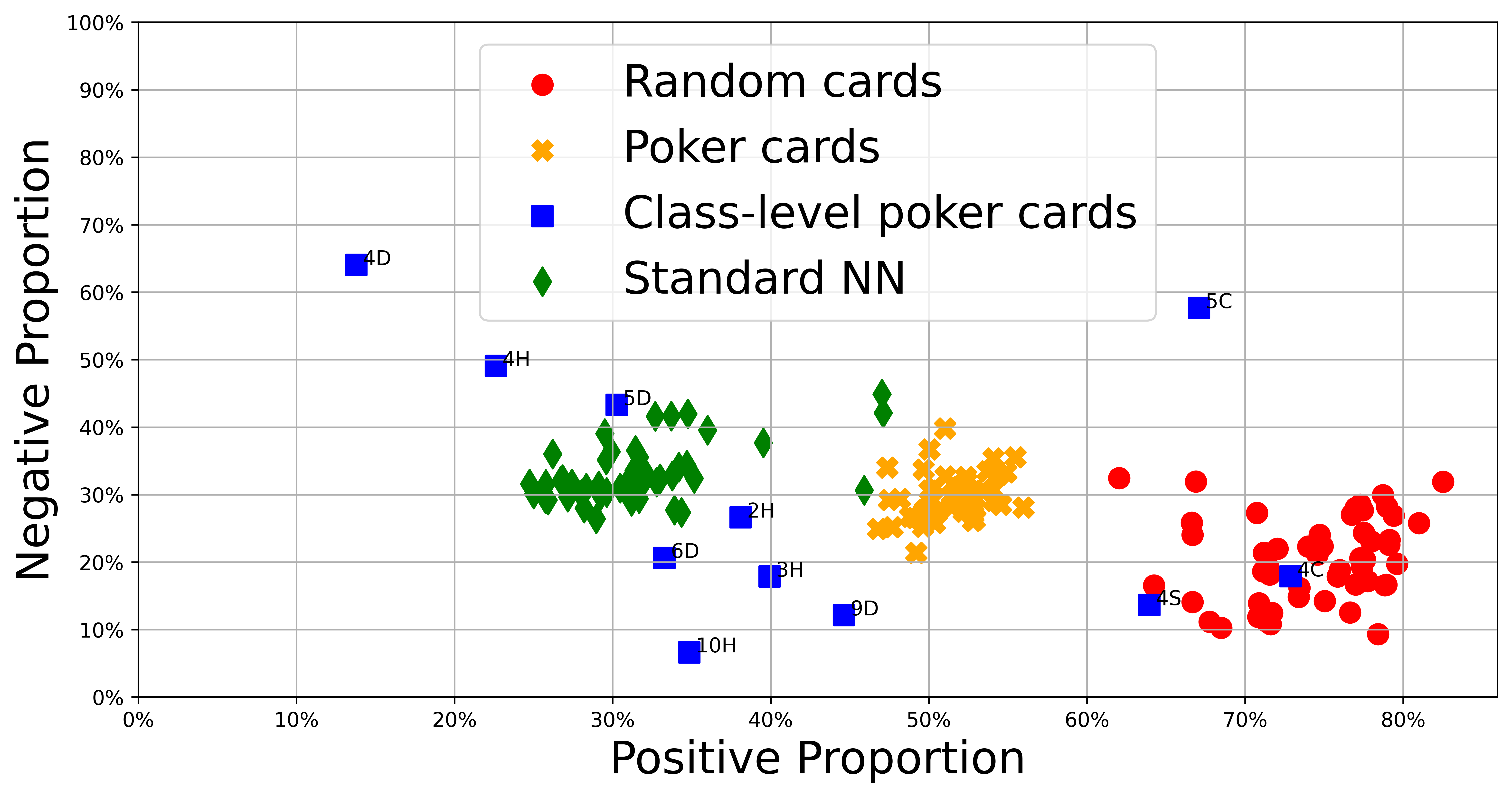
To analyse if our playing card models are applying relevance to semantically meaningful input features with a quantitative metric, we can measure the proportion of relevance applied to concepts’ visual representations. If the proportion of positive relevance is high, and the proportion of negative relevance is low, then we can argue the model has learned a semantically meaningful concept mapping. We compare our random cards, poker cards, class-level poker cards, and standard NN models in Figure 3 with averaged proportions over 5 models for each dataset variant. Each point represents a single concept. Relevance on the background is discarded as it plays no part in predicting concepts. The plot shows three distinct clusters, one for each of random cards, poker cards and the standard NN. Random cards have the highest proportion of positive relevance and the lowest proportion of negative relevance. Poker cards have less positive relevance and more negative relevance but still show an improvement from the standard NN. Combining this plot with the saliency maps we saw in Figure 1 confirms the CBMs have learned to apply relevance to semantically meaningful input features for both random cards and poker cards, although less so for poker cards. As random cards have concepts selected at random, whereas poker cards concepts are restricted to what the downstream task permits (e.g. Straight Flush requires three cards of the same suit and incriminating values), this plot shows how a reduction of concept correlation benefits CBMs learning semantic concept mappings. In this case, caused by the downstream task. The points for class-level poker cards are not clustered together. Most concepts have a low proportion of relevance, meaning a semantically meaningful concept mapping has not been learned. A few concepts however, Four of Spades, Four of Clubs and Five of Clubs have a high proportion of positive relevance. For the concepts Four of Spades and Four of Clubs, this confirms what we saw in Figure 2(a), that a semantically meaningful concept mapping has been learned. The same cannot be said for the concept Five of Clubs as all saliency maps for concepts predicted as present when this concept is in the input image, apply positive relevancy to this concept’s semantic input features (see Figure 2(b)), inflating the positive proportion we see. Class-level poker cards reveal the challenge of engineering a dataset with enough constraints for the model to learn semantically meaningful concept mappings. Even though the concepts Four of Spades and Four of Clubs show it possible for a CBM to learn semantically meaningful concept mappings with class-level concepts, the consistency in relevancy proportions with random cards and poker cards shows the advantage instance-level concepts can provide.
To evaluate CBM’s ability to map semantic input features to concepts in a real-world setting we have trained CBMs on the dataset CheXpert. As the dataset domain is on chest X-rays, most images will contain the relevant input features to map to concept annotations. Essentially as all concepts represent visual signs in the chest region, and all images are chest X-rays, then concepts should have a visual representation in the corresponding input image. As uncertain or missing concepts are set to present, there will be some noise in the training data and we may assume there is some additional noise caused by the annotations originally being generated using an automated labeller Irvin et al. (2019). For our results in Figure 4, we are using the saliency mapping technique Guided Grad-CAM Selvaraju et al. (2017) and our models trained on instance-level CheXpert. To validate that the models have mapped concepts to intended input features we are using ground truth segmentations from Saporta et al. (2022). These were created by two board-certified radiologists and ensure our conclusions are made w.r.t. expert opinion. Our results show concepts trained on instance-level CheXpert can map concepts to semantic input features for both models trained with the independent/sequential method 4(a) and joint method 4(b). The concepts for Edema, Consolidation, Atelectasis and Pleural effusion all should be observable with signs in the lungs while Cardiomegaly is observed by an enlarged heart and thus should either highlight the heart or areas around the heart. From the samples we show, most concepts map to features within the ground truth segmentation such as the saliency maps for the concepts Atelectasis and Edema. The saliency maps for the concept Consolidation maps to the incorrect lung which may be considered a reasonable error to make, the model is still mapping to the correct organ. As for the concept Cardiomegaly, the model still maps to the lungs, but most relevance is outside of the ground truth segmentation. Instance-level CheXpert saliency maps are distinctly different to each other and do not appear to be using the same input features for every concept prediction, unlike class-level CheXpert as we see in Figure 5 where all concept saliency maps highlight similar input features irrespective of the concept being predicted.
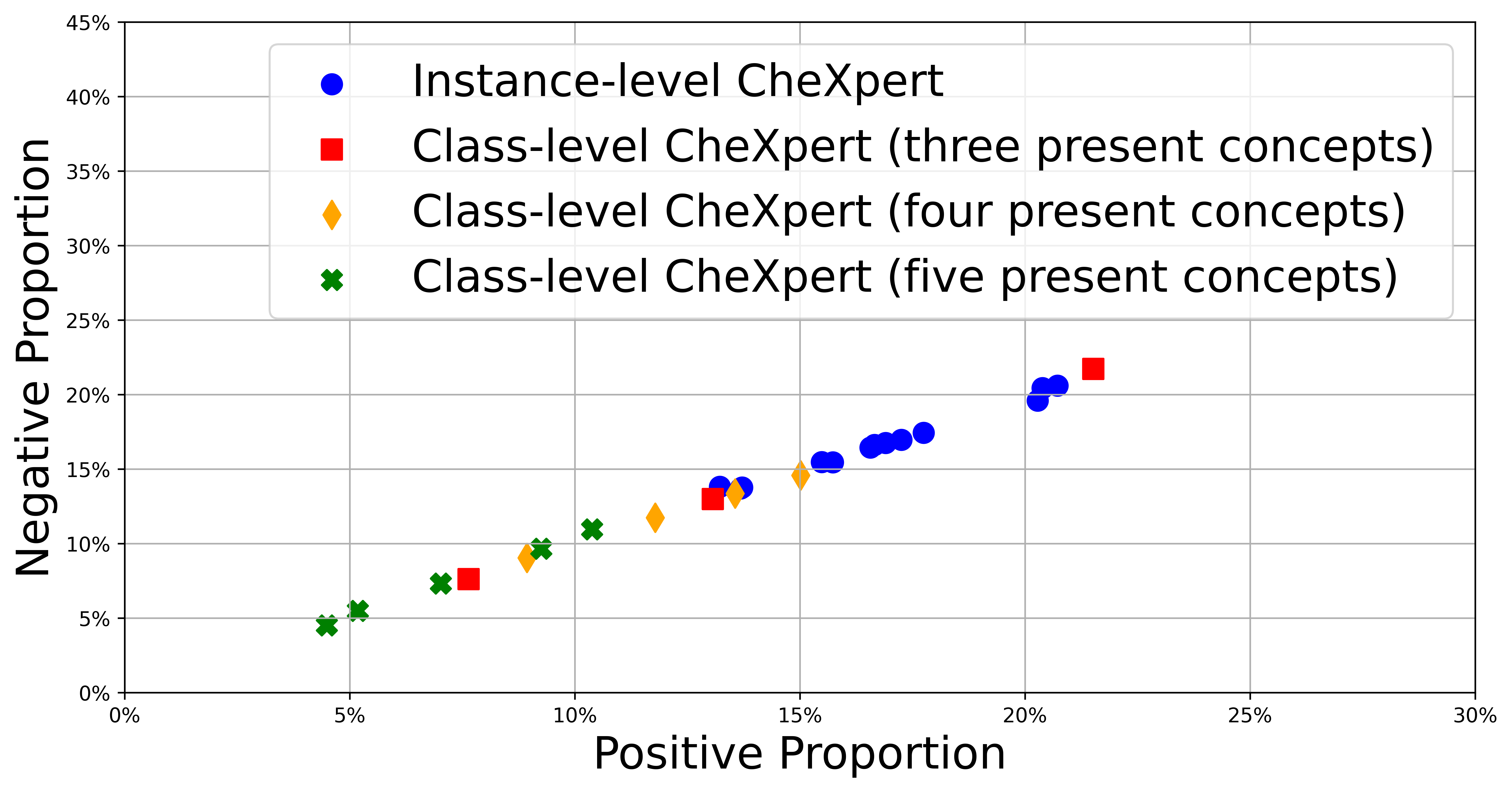
The proportion of relevance using our joint trained CheXpert models is shown in Figure 6. The maximum positive saliency is much lower than playing cards, topping out just over 20% and the concepts for instance-level CheXpert are not clustered but instead form a line. As discussed by Saporta et al. (2022), the most accurate concepts tend to be larger in size which could explain this. We are however more interested in the differences between instance-level CheXpert and class-level CheXpert. Instance-level CheXpert generally outperforms class-level CheXpert at mapping input features to concept segmentations. Most class-level concepts have a very little positive proportion of relevance located to the ground truth segmentations. We can therefore take away the concept annotations for instance-level CheXpert can confine models to learn semantic input features and further reinforces the need to avoid training CBMs on concepts that are only present together.
5.2 Concept Purity
If we can train CBMs to learn semantically meaningful input features we may also expect an improvement in concept purity. We measure concept purity using the Oracle Impurity Score (OIS) Espinosa Zarlenga et al. (2023). Our configuration uses a helper model formed of a two-layer ReLU multi-layer perceptron with 32 activations in its hidden layer. Concept representation quality is defined as purity, whether a learned concept representation has a predictive power similar to what would be expected from ground truth labels. OIS is the divergence of two matrices; the predictability of ground truth concepts w.r.t. one another, the oracle matrix, and the predictability of ground truth concepts from learned concepts, the purity matrix. If OIS results in a value of 0 then learned concepts do not encode any more or less information than is required to predict themselves whereas a value of 1 means each learned concept can predict all other concepts.
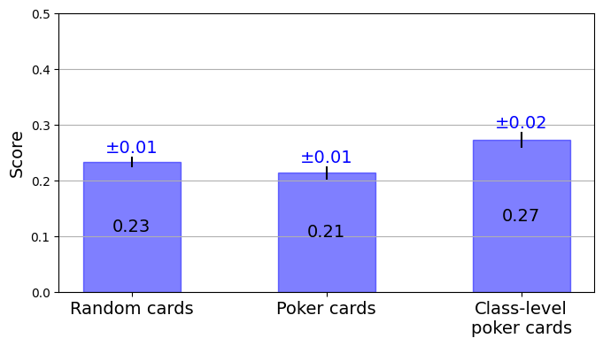
OIS results for poker cards, random cards (both tested with the poker cards dataset), and class-level poker cards are shown in Figure 7. We cannot use OIS with our CheXpert models as OIS makes use of AUC. As the test dataset split for CheXpert has a limited number of samples, a few concepts have one or zero annotations representing the concepts as being present. Results for playing cards are averaged over 5 training runs using the independent training method with each set of weights used to generate an OIS value 3 times. Models trained on poker cards show a marginal improvement over random cards with class-level poker cards having the highest OIS value. These results may appear unexpected given how random cards should have no inter-concept predictability, unlike poker cards and class-level poker cards. OIS however is w.r.t. the expected impurities that exist in the dataset. If a number of ground truth concepts have a high correlation and the concept representations have the same correlation then the OIS metric will show low impurity. If however the concept representations capture different correlations then the OIS metric will show higher impurities.
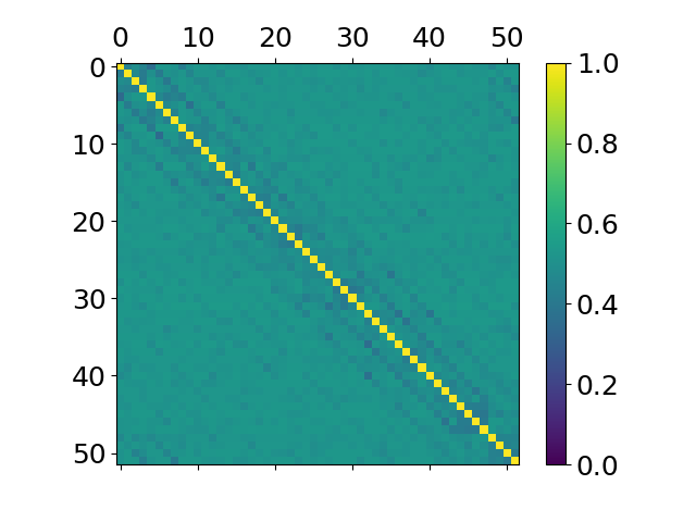
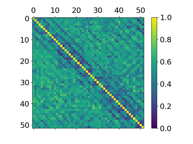
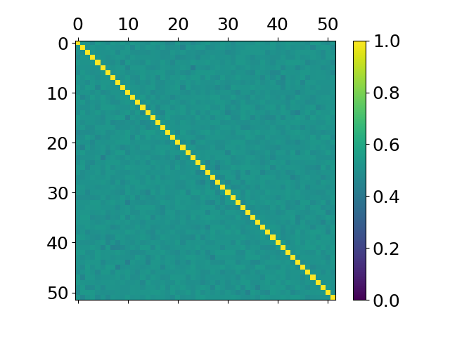
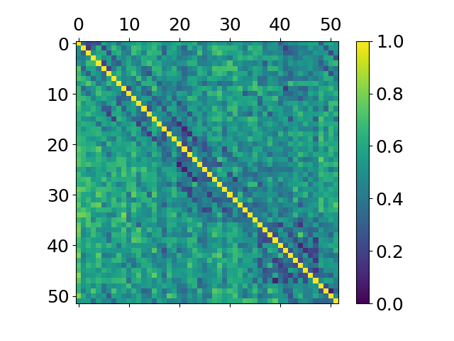
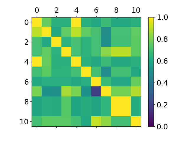
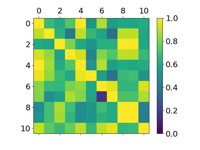
To expand on the OIS scores we have visualised the two matrices from the OIS value for each dataset variation, shown in Figure 8. Each coordinate in these matrices shows the predictability for one concept predicting another concept as an AUC value. All oracle matrices show a strong predictability for each concept predicting itself, which is to be expected. The oracle matrix for Figure 8(a) shows additional diagonals with AUC values lower than 0.5, where concepts in the dataset have information for non-random inter-concept predictability. These diagonals are not present in the random concepts dataset, Figure 8(c). Looking at the purity matrices for playing cards, Figure 8(b) and Figure 8(d), the additional diagonals of inter-concept predictability continues for poker cards but there is a distinct reduction with random cards. Remembering the OIS value can either show extra information or a lack of information w.r.t. the expectation from the dataset, the higher value for random cards in Figure 7 is likely showing a lack of expected information. For class-level poker cards the oracle matrix, Figure 8(e), shows mostly random inter-concept predictability apart from for a few concepts. These concepts are those that are only used for a single downstream task. The purity matrices have many more concepts with increased inter-concept predictability although they are all located to concepts within a few steps from the concepts with non-random inter-concept predictability in Figure 8(e). This shows the models have encoded extra information for each concept than is required, for instance, the concepts Six or Nine of Diamonds (index 8 and 9) are only present when the Four of Diamonds (index 3) is present. Therefore the concepts Six or Nine will never be present if the Four of Clubs (index 2) is present.
6 Discussion and Conclusion
In this paper, we realise the original promise of CBM’s inherent interpretability by training models which map concepts to semantically meaningful input features. This benefits inherent interpretability as we can be sure the model is predicting concepts for the right reasons, and not due to some unintended dataset configuration. If a CBM makes predictions using semantically mapped input features, we can argue the model will be easier to build trust with as concept predictions will use the expected input features from a human perspective. We achieved semantically meaningful concept mappings by training CBMs with accurate concept annotations and with a high variety of concepts that are present together. This differs from the previously analysed CUB dataset with class-level concepts which cannot account for visual changes in the input images. The semantically meaningful concept mappings do not come from the use of class or instance-level concepts, but instead from ensuring if a concept is annotated as present in the dataset then it is visually present in the corresponding image and the occurrence of concepts in the dataset do not create unintended correlations. We however demonstrate it’s easier to achieve semantically meaningful concept mappings with instance-level concept annotations.
We show how learned concept representations can encode correlations between concepts from the dataset which may lead to concepts being predicted based on the presence or absence of other concepts. If this is to be avoided the correlation of concepts in the dataset should be considered, and if the downstream task restricts this, can be avoided by splitting the training of the two model parts to learn concepts and the downstream task separately.
Future research regarding the representations CBMs learn should focus on CBMs trained on larger datasets. Although Oikarinen et al. (2023) shows how large language models and CLIP can be used to train an iteration of CBMs, removing the need for manual concept annotations, the semantic mapping from concepts to input features remains unclear. Ensuring concept annotations have a semantic mapping, even for large or machine-generated datasets, or including another constraint to achieve semantically meaningful concept mappings, should be a priority for ensuring inherent interpretability and human trust can be achieved.
References
- Bach et al. [2015] Sebastian Bach, Alexander Binder, Grégoire Montavon, Frederick Klauschen, Klaus-Robert Müller, and Wojciech Samek. On pixel-wise explanations for non-linear classifier decisions by layer-wise relevance propagation. PLOS ONE, 10(7):1–46, 07 2015.
- Bengio et al. [2013] Y. Bengio, Aaron Courville, and Pascal Vincent. Representation learning: A review and new perspectives. IEEE transactions on pattern analysis and machine intelligence, 35:1798–1828, 08 2013.
- Biewald [2020] Lukas Biewald. Experiment tracking with weights and biases, 2020. Software available from wandb.com.
- Chauhan et al. [2023] Kushal Chauhan, Rishabh Tiwari, Jan Freyberg, Pradeep Shenoy, and Krishnamurthy Dvijotham. Interactive concept bottleneck models. Proceedings of the AAAI Conference on Artificial Intelligence, 37(5):5948–5955, Jun. 2023.
- Espinosa Zarlenga et al. [2023] Mateo Espinosa Zarlenga, Pietro Barbiero, Zohreh Shams, Dmitry Kazhdan, Umang Bhatt, Adrian Weller, and Mateja Jamnik. Towards robust metrics for concept representation evaluation. Proceedings of the AAAI Conference on Artificial Intelligence, 37(10):11791–11799, Jun. 2023.
- Furby et al. [2023] Jack Furby, Daniel Cunnington, Dave Braines, and Alun Preece. Towards a deeper understanding of concept bottleneck models through end-to-end explanation. R2HCAI: The AAAI 2023 Workshop on Representation Learning for Responsible Human-Centric AI, 2023.
- Huang et al. [2017] Gao Huang, Zhuang Liu, Laurens van der Maaten, and Kilian Q. Weinberger. Densely connected convolutional networks. In Proceedings of the IEEE Conference on Computer Vision and Pattern Recognition (CVPR), July 2017.
- Irvin et al. [2019] Jeremy Irvin, Pranav Rajpurkar, Michael Ko, Yifan Yu, Silviana Ciurea-Ilcus, Chris Chute, Henrik Marklund, Behzad Haghgoo, Robyn Ball, Katie Shpanskaya, Jayne Seekins, David A. Mong, Safwan S. Halabi, Jesse K. Sandberg, Ricky Jones, David B. Larson, Curtis P. Langlotz, Bhavik N. Patel, Matthew P. Lungren, and Andrew Y. Ng. Chexpert: A large chest radiograph dataset with uncertainty labels and expert comparison. Proceedings of the AAAI Conference on Artificial Intelligence, 33(01):590–597, Jul. 2019.
- Kazhdan et al. [2021] Dmitry Kazhdan, Botty Dimanov, Helena Andres Terre, Mateja Jamnik, Pietro Liò, and Adrian Weller. Is disentanglement all you need? comparing concept-based & disentanglement approaches. RAI workshop at The Ninth International Conference on Learning Representations 2021, 2021.
- Kingma and Ba [2014] Diederik Kingma and Jimmy Ba. Adam: A method for stochastic optimization. International Conference on Learning Representations, 12 2014.
- Koh et al. [2020] Pang Wei Koh, Thao Nguyen, Yew Siang Tang, Stephen Mussmann, Emma Pierson, Been Kim, and Percy Liang. Concept bottleneck models. In Hal Daumé III and Aarti Singh, editors, Proceedings of the 37th International Conference on Machine Learning, volume 119 of Proceedings of Machine Learning Research, pages 5338–5348. PMLR, 13–18 Jul 2020.
- Mahinpei et al. [2021] A. Mahinpei, J. Clark, I. Lage, F. Doshi-Velez, and P. WeiWei. Promises and pitfalls of black-box concept learning models. In proceeding at the International Conference on Machine Learning: Workshop on Theoretic Foundation, Criticism, and Application Trend of Explainable AI,, volume 1, pages 1–13, 2021.
- Marconato et al. [2022] Emanuele Marconato, Andrea Passerini, and Stefano Teso. Glancenets: Interpretabile, leak-proof concept-based models, 05 2022.
- Margeloiu et al. [2021] Andrei Margeloiu, Matthew Ashman, Umang Bhatt, Yanzhi Chen, Mateja Jamnik, and Adrian Weller. Do concept bottleneck models learn as intended? ICLR 2021 Workshop on Responsible AI, 2021.
- Miller [2019] Tim Miller. Explanation in artificial intelligence: Insights from the social sciences. Artificial Intelligence, 267:1–38, 2019.
- Montavon et al. [2019] Grégoire Montavon, Alexander Binder, Sebastian Lapuschkin, Wojciech Samek, and Klaus-Robert Müller. Layer-Wise Relevance Propagation: An Overview, pages 193–209. Springer International Publishing, 09 2019.
- Oikarinen et al. [2023] Tuomas Oikarinen, Subhro Das, Lam M. Nguyen, and Tsui-Wei Weng. Label-free concept bottleneck models. In The Eleventh International Conference on Learning Representations, 2023.
- Radford et al. [2021] Alec Radford, Jong Wook Kim, Chris Hallacy, Aditya Ramesh, Gabriel Goh, Sandhini Agarwal, Girish Sastry, Amanda Askell, Pamela Mishkin, Jack Clark, Gretchen Krueger, and Ilya Sutskever. Learning transferable visual models from natural language supervision. In International Conference on Machine Learning, 2021.
- Ribeiro et al. [2016] Marco Ribeiro, Sameer Singh, and Carlos Guestrin. “why should I trust you?”: Explaining the predictions of any classifier. In Proceedings of the 2016 Conference of the North American Chapter of the Association for Computational Linguistics: Demonstrations, pages 97–101, San Diego, California, June 2016. Association for Computational Linguistics.
- Saporta et al. [2022] Adriel Saporta, Xiaotong Gui, Ashwin Agrawal, Anuj Pareek, Steven Q. H. Truong, Chanh D. T. Nguyen, Van-Doan Ngo, Jayne Seekins, Francis G. Blankenberg, Andrew Y. Ng, Matthew P. Lungren, and Pranav Rajpurkar. Benchmarking saliency methods for chest x-ray interpretation. Nature Machine Intelligence, 4, 2022.
- Selvaraju et al. [2017] Ramprasaath R. Selvaraju, Michael Cogswell, Abhishek Das, Ramakrishna Vedantam, Devi Parikh, and Dhruv Batra. Grad-cam: Visual explanations from deep networks via gradient-based localization. In 2017 IEEE International Conference on Computer Vision (ICCV), pages 618–626, 2017.
- Simonyan and Zisserman [2015] Karen Simonyan and Andrew Zisserman. Very deep convolutional networks for large-scale image recognition. In International Conference on Learning Representations, 2015.
- Sundararajan et al. [2017] Mukund Sundararajan, Ankur Taly, and Qiqi Yan. Axiomatic attribution for deep networks. In Proceedings of the 34th International Conference on Machine Learning - Volume 70, ICML’17, page 3319–3328. JMLR.org, 2017.
- Wah et al. [2011] C. Wah, S. Branson, P. Welinder, P. Perona, and S. Belongie. The Caltech-UCSD Birds-200-2011 Dataset. Technical Report CNS-TR-2011-001, California Institute of Technology, 2011.
- Yang et al. [2023] Yue Yang, Artemis Panagopoulou, Shenghao Zhou, Daniel Jin, Chris Callison-Burch, and Mark Yatskar. Language in a bottle: Language model guided concept bottlenecks for interpretable image classification. In Proceedings of the IEEE/CVF Conference on Computer Vision and Pattern Recognition (CVPR), pages 19187–19197, June 2023.
- Ye et al. [2020] Wenwu Ye, Jin Yao, Hui Xue, and Yi Li. Weakly supervised lesion localization with probabilistic-cam pooling, 2020.
Appendix A Experiments set-up
In this section, we provide further details on datasets, model architectures and training methods used in this paper. All experiments were run on a workstation with a single 24GB NVIDIA Quadro RTX 6000 GPU, Intel(R) Core(TM) i9-10900K CPU @ 3.70GHz and 64GB of system memory. The machine runs Ubuntu 22.04.3 LTS. We estimate around 500 hours are required to train models and run all experiments, which includes training each model 5 times on random seeds. All random seeds were selected using the shuf command to select a number between 0 and 1000.
A.1 Models and training
Playing cards: All playing card models use a VGG-11 architecture with batch normalisation Simonyan and Zisserman [2015] for the model part. The model part used two linear layers with a ReLU activation function. Between the two model parts, we used a sigmoid function. During training, we evaluate these models w.r.t. the combined concept and downstream loss. We detail average model accuracies in Table 1. For experiments that used a single model (e.g. saliency map generation), we selected the model with the highest concept accuracy. These are detailed in Table 2.
| Training method | Dataset |
Average
concept accuracy (%) |
Concept
standard deviation |
Average task accuracy (%) | Task standard deviation |
|---|---|---|---|---|---|
| Independent | Random cards | 99.943 | 0.008 | 99.174 | 0.09 |
| Sequential | Random cards | 99.921 | 0.044 | 97.457 | 0.76 |
| Independent | Poker cards | 99.957 | 0.005 | 99.421 | 0.034 |
| Sequential | Poker cards | 99.917 | 0.051 | 98.802 | 0.277 |
| Joint | Poker cards | 99.867 | 0.046 | 96.005 | 0.213 |
| Independent | Class-level poker cards | 99.98 | 0.014 | 99.96 | 0.039 |
| Sequential | Class-level poker cards | 99.98 | 0.014 | 99.953 | 0.045 |
| Joint | Class-level poker cards | 100 | 0 | 100 | 0 |
| Standard NN | Poker cards | 50.25 | 1.31 | 67.137 | 0.584 |
| Model | Dataset | Concept accuracy (%) |
|---|---|---|
| Independent & Sequential | Random cards | 99.961 |
| Independent & Sequential | Poker cards | 99.961 |
| Independent & Sequential | Class-level poker cards | 99.997 |
| Joint | Poker cards | 99.936 |
| Standard NN | Poker cards | 52.717 |
We used Weights and Biases Sweeps Biewald [2020] to find optimal hyperparameters for training each of our models on the playing cards dataset. This was configured with a Bayesian search method to optimise the parameters. These were; starting learning rate (between 0.1 and 0.001), optimizer (between Adam Kingma and Ba [2014] and stochastic gradient descent (SGD)), learning rate patience (between 3, 5, 10 and 15 epochs of no improvement in loss) and theta value (A value used with joint training to balance concept and downstream task loss). Sweeps were run for each of the dataset variants and CBM training. Each sweep ran until we stopped seeing improvements in the model accuracy, about 30 iterations per sweep. The final hyperparameters we used are in Table 3.
| Training method & Dataset | Learning rate | Optimizer | Batch size | Learning rate patience | Theta | Epochs |
|---|---|---|---|---|---|---|
| Independent & sequential - Random cards | 0.03 | SGD | 32 | 15 | N/A | 200 |
| Independent & sequential - Poker cards | 0.02 | SGD | 32 | 15 | N/A | 200 |
| Independent & sequential - Class-level poker cards | 0.0825 | SGD | 32 | 3 | N/A | 100 |
| Independent - Random cards | 0.01 | Adam | 32 | 5 | N/A | 200 |
| Independent - Poker cards | 0.01 | Adam | 32 | 5 | N/A | 200 |
| Independent - Class-level poker cards | 0.064 | Adam | 32 | 5 | N/A | 100 |
| Sequential - Random cards | 0.059 | Adam | 32 | 5 | N/A | 200 |
| Sequential - Poker cards | 0.046 | Adam | 32 | 15 | N/A | 200 |
| Sequential - Class-level poker cards | 0.0846 | Adam | 32 | 10 | N/A | 100 |
| Joint - Poker cards | 0.025 | SGD | 32 | 15 | 0.98 | 300 |
| Joint - Class-level poker cards | 0.0398 | SGD | 32 | 15 | 0.867 | 100 |
| Standard NN - Poker cards | 0.088 | SGD | 32 | 15 | 0 | 300 |
CheXpert Irvin et al. [2019]: Our CheXpert models use a Densenet121 architecture Huang et al. [2017] for the model part and pre-trained weights, trained on Imagenet. The model part used two linear layers with a ReLU activation function. Between the two model parts, we used a sigmoid function. We evaluated these models w.r.t. Area Under the receiver operating characteristic Curve (AUC) for concepts. Averaged model performance is shown in Table 4. The best model accuracies are shown in Table 5 and AUC values in Table 6. These models were selected as they had the highest AUC values. Model training hyperparameters are listed in Table 7. We do not display AUC values for the concept ‘Fracture’ as there are no positive samples for this concept in the test dataset split.
A.2 Datasets
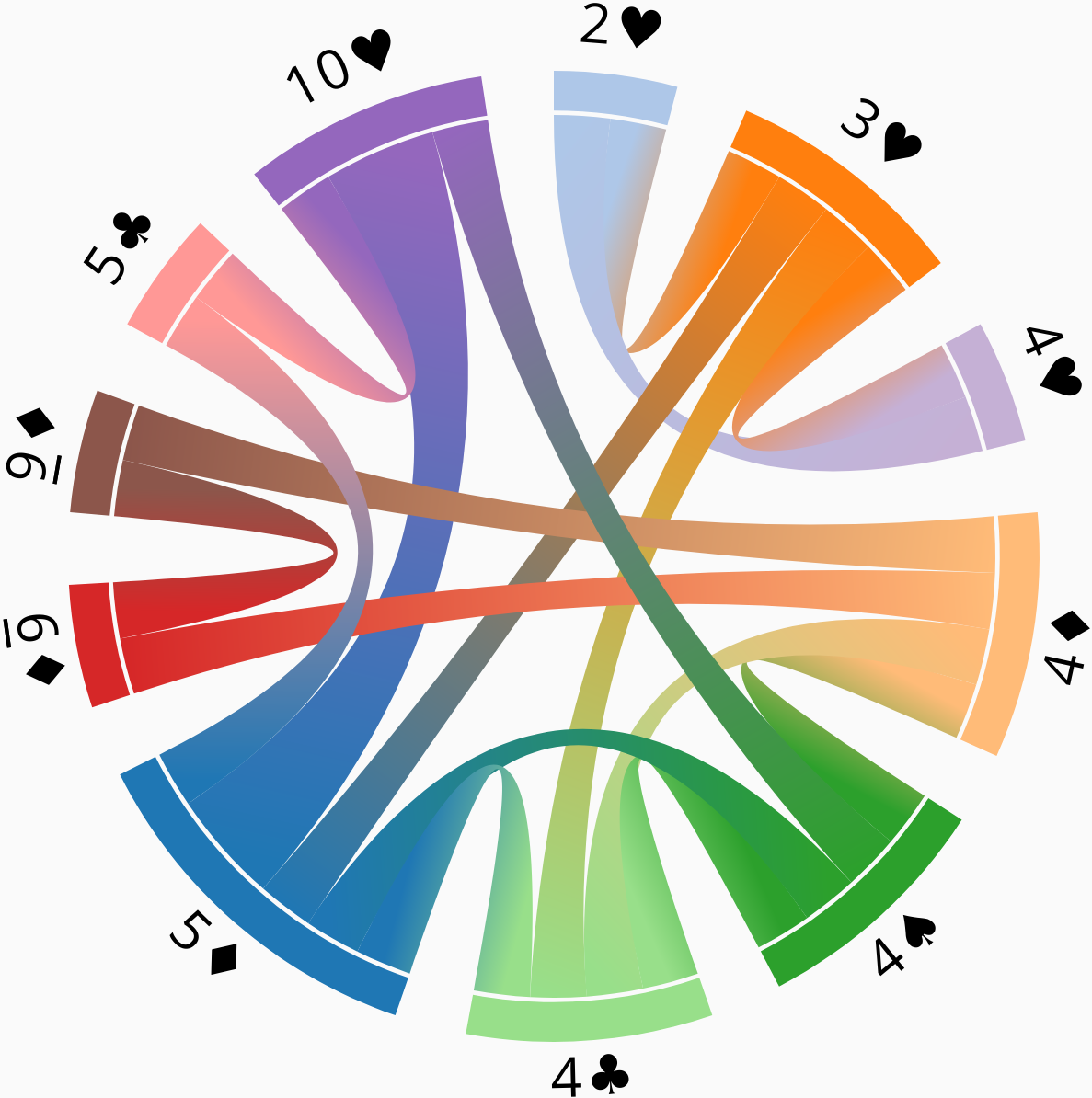
Playing cards: Playing cards is a synthetic dataset where each sample has either one or three playing cards placed on a random background. Each sample has annotations for a downstream task classification, a series of concepts, and playing card coordinates. Playing cards are placed in a random location on the background image, with a random size and rotation, but with the constraint that each playing card is fully visible. If three cards are in a sample, then they are placed in a line. We include four versions of the dataset; single playing card which includes one playing card and class-level concepts representing the suit and rank of the card, random cards which have three random playing cards, poker cards which have three playing cards that are selected based on a hand rank in the game Three Card Poker, and class-level poker cards which is similar to poker cards but has a reduced set of concepts. Random cards and poker cards have instance-level concepts with concepts representing cards present in each sample. Each variation has 10,000 samples where 70% are training images and 30% are testing/validation images. Example images are shown in Figure 9. Code to generate the dataset is publicly available222Playing cards dataset generator: Available in camera-ready submission. The concepts in class-level poker cards represent playing cards but instead of 52 concepts, class-level poker cards reduce this to 11 concepts. These concepts are arranged such that some concepts are only used for one downstream task class while others are used for many. The mapping between concepts which appear in the same images is shown in Figure 10.
In this paper, we transform training samples with a random flip, both horizontal and vertical, apply a colour jitter to the brightness, contrast, saturation and hue, and randomly convert to grey scale. Samples are scaled to 299 by 299 pixels.
CheXpert Irvin et al. [2019]: CheXpert is an image dataset in the domain of chest X-rays. It has 14 signs, of which we have used 13 for concepts with the 14 (No findings) as the downstream task. The dataset contains 224,316 X-ray images. We use the official dataset splits from Irvin et al. [2019]. The original validation split was used as a holdout test split with only frontal-view images kept, 202 in total. We have configured the dataset to use U-ones annotations which sets any missing or uncertain annotations to 1 representing the sign as being present. For all samples in the training set, CheXpert used an automated annotator to label the 14 annotations from radiology reports. The test set was annotated by the consensus of 5 board-certified radiologists. During training, samples are randomly rotated by up to 15 degrees, translated by up to 5% of the overall image width and scaled by up to 5%. All samples are resized to 512 by 512 pixels.
| Training method |
Dataset
version |
Concept
accuracy (%) |
Concept
standard deviation |
Task accuracy (%) | Task standard deviation |
|---|---|---|---|---|---|
| Sequential | Instance-level | 75.971 | 1.77 | 0.865 | 0.001 |
| Joint | Instance-level | 77.659 | 1.578 | 0.883 | 0.009 |
| Sequential | Class-level with 3 present concepts | 58.044 | 9.141 | 62.414 | 0.023 |
| Sequential | Class-level with 4 present concepts | 62.268 | 10.004 | 36 | 0.014 |
| Sequential | Class-level with 5 present concepts | 61.971 | 6.754 | 36.571 | 0.021 |
| Joint | Class-level with 3 present concepts | 56.211 | 2.098 | 95.517 | 0.008 |
| Joint | Class-level with 4 present concepts | 60.569 | 8.727 | 95.429 | 0.034 |
| Joint | Class-level with 5 present concepts | 59.952 | 3.932 | 0.967 | 0.032 |
| Model | Dataset version | Concept accuracy (%) |
|---|---|---|
| Sequential | Instance-level CheXpert | 75.659 |
| Joint | Instance-level CheXpert | 78.668 |
| Sequential | Class-level CheXpert with 3 present concepts | 71.598 |
| Sequential | Class-level CheXpert with 4 present concepts | 68.71 |
| Sequential | Class-level CheXpert with 5 present concepts | 64.623 |
| Concept |
Sequential instance-level CheXpert |
Joint instance-level CheXpert |
Joint class-Level CheXpert with 3 present concepts |
Joint class-Level CheXpert with 4 present concepts |
Joint class-Level CheXpert with 5 present concepts |
|---|---|---|---|---|---|
| Enlarged cardiomediastium | 0.525 | 0.547 | N/A | N/A | N/A |
| Cardiomegaly | 0.831 | 0.879 | N/A | N/A | N/A |
| Lung opacity | 0.933 | 0.912 | 0.998 | 1.0 | 1.0 |
| Lung lesion | 0.127 | 0.138 | N/A | N/A | N/A |
| Edema | 0.932 | 0.954 | N/A | 1.0 | N/A |
| Consolidation | 0.867 | 0.847 | N/A | N/A | 0.875 |
| Pneumonia | 0.572 | 0.628 | N/A | N/A | N/A |
| Atelectasis | 0.795 | 0.776 | N/A | N/A | 1.0 |
| Pneumothorax | 0.795 | 0.795 | N/A | N/A | N/A |
| Pleural effusion | 0.930 | 0.931 | 0.998 | 1.0 | 1.0 |
| Plaural other | 0.142 | 0.143 | N/A | N/A | N/A |
| Support devices | 0.966 | 0.959 | 0.998 | 1.0 | 1.0 |
| Training method | Learning rate | Optimizer | Batch size | Learning rate patience | Theta | Epochs |
|---|---|---|---|---|---|---|
| Independent & sequential | 0.0001 | Adam | 14 | 0.1 | N/A | 3 |
| Sequential | 0.0001 | Adam | 14 | 0.1 | N/A | 3 |
| Joint | 0.0001 | Adam | 14 | 0.1 | 0.99 | 3 |
Appendix B Experiments and results
B.1 Playing cards
We show additional concept saliency map results for our instance-level playing card models in Figure 11 and 12, 13, and 14. We provide examples of all downstream task classes for class-level poker card saliency maps to variations between all concept predictions. These can be seen in Figure 15, 16, 17, 18, 19 and 20. We used three explanation techniques; LPR, IG with a smoothgrad noise tunnel, and IG with a smoothgrad squared noise tunnel. For LRP we used the rules LRP-, where and , for the first four convolutional layers of the model from the input, LRP- for the next four convolutional layers and LRP-0 for the top three linear layers. IG with a smoothgrad noise tunnel is configured to use 25 randomly generated samples and a standard deviation of 0. Most saliency maps focus on the playing card that maps semantically to its corresponding concept. All saliency maps generated with LRP show positive relevancy attributed to the correct playing card for each concept to satisfy semantically meaningful feature mapping, while both IG variations show good localisation. IG with a smoothgrad squared noise tunnel applies little relevance in general and highlights a different card for the concept King of Hears in Figure 13.
B.2 CheXpert
We show additional saliency maps results for instance-level CheXpert in Figure 21, 22, 23 and 24 using three explanation techniques; IG with a smoothgrad noise tunnel, and IG with a smoothgrad squared noise tunnel and GradCAM Selvaraju et al. [2017]. IG with a smoothgrad noise tunnel and IG with a smoothgrad squared noise tunnel is configured to use 25 randomly generated samples and a standard deviation of 0.2. For the most part, relevance is localised but fairly noisy, especially for IG. For a number of concepts, saliency is also not within ground truth segmentations (the areas highlighted with green). Each saliency map is distinctly different from concept to concept so we can tell the model is not using the same input features to predict each concept. Class-level CheXpert in Figure 25, 26, 27, 28, 29 and 30 tell a different story as all concepts share very similar saliency maps and thus, the model is using the same input features to predict all concepts.
| input | |||
| King of Hearts | Nine of Diamonds | Ace of Clubs | |
|
LRP |
|||
|
IG with Smoothgrad |
|||
|
IG with Smoothgrad squared |
|||
| 1.0 | 0.99998 | 0.99991 |
| input | |||
| Ace of Spades | Two of Spades | Three of Spades | |
|
LRP |
|||
|
IG with Smoothgrad |
|||
|
IG with Smoothgrad squared |
|||
| 1.0 | 1.0 | 1.0 |
| input | |||
| King of Hearts | Nine of Diamonds | Ace of Clubs | |
|
LRP |
|||
|
IG with Smoothgrad |
|||
|
IG with Smoothgrad squared |
|||
| 1.0 | 1.0 | 0.99999 |
| input | |||
| Ace of Spades | Two of Spades | Three of Spades | |
|
LRP |
|||
|
IG with Smoothgrad |
|||
|
IG with Smoothgrad squared |
|||
| 1.0 | 1.0 | 0.99985 |
| input | |||
| King of Hearts | Nine of Diamonds | Ace of Clubs | |
|
LRP |
|||
|
IG with Smoothgrad |
|||
|
IG with Smoothgrad squared |
|||
| 0.99999 | 0.98979 | 1.0 |
| input | |||
| Ace of Spades | Two of Spades | Three of Spades | |
|
LRP |
|||
|
IG with Smoothgrad |
|||
|
IG with Smoothgrad squared |
|||
| 0.45868 | 1.0 | 0.99996 |
| input | |||
| King of Hearts | Nine of Diamonds | Ace of Clubs | |
|
LRP |
|||
|
IG with Smoothgrad |
|||
|
IG with Smoothgrad squared |
|||
| 0.44373 | 0.3453 | 0.82097 |
| input | |||
| Ace of Spades | Two of Spades | Three of Spades | |
|
LRP |
|||
|
IG with Smoothgrad |
|||
|
IG with Smoothgrad squared |
|||
| 1.0 | 1.0 | 1.0 |
| input | |||
| Two of Hearts | Three of Hearts | Four of Hearts | |
|
LRP |
|||
|
IG with Smoothgrad |
|||
|
IG with Smoothgrad squared |
|||
| 1.0 | 1.0 | 1.0 |
| input | |||
| Two of Hearts | Three of Hearts | Four of Hearts | |
|
LRP |
|||
|
IG with Smoothgrad |
|||
|
IG with Smoothgrad squared |
|||
| 1.0 | 1.0 | 1.0 |
| input | |||
| Four of Clubs | Four of Diamonds | Four of Spades | |
|
LRP |
|||
|
IG with Smoothgrad |
|||
|
IG with Smoothgrad squared |
|||
| 1.0 | 1.0 | 1.0 |
| input | |||
| Four of Clubs | Four of Diamonds | Four of Spades | |
|
LRP |
|||
|
IG with Smoothgrad |
|||
|
IG with Smoothgrad squared |
|||
| 1.0 | 1.0 | 1.0 |
| input | |||
| Three of Hearts | Four of Clubs | Five of Diamonds | |
|
LRP |
|||
|
IG with Smoothgrad |
|||
|
IG with Smoothgrad squared |
|||
| 0.99994 | 0.99999 | 0.99976 |
| input | |||
| Three of Hearts | Four of Clubs | Five of Diamonds | |
|
LRP |
|||
|
IG with Smoothgrad |
|||
|
IG with Smoothgrad squared |
|||
| 0.99999 | 0.99998 | 0.9999 |
| input | |||
| Four of Diamonds | Six of Diamonds | Nine of Diamonds | |
|
LRP |
|||
|
IG with Smoothgrad |
|||
|
IG with Smoothgrad squared |
|||
| 0.99996 | 0.99999 | 0.99999 |
| input | |||
| Four of Diamonds | Six of Diamonds | Nine of Diamonds | |
|
LRP |
|||
|
IG with Smoothgrad |
|||
|
IG with Smoothgrad squared |
|||
| 0.99999 | 1.0 | 1.0 |
| input | |||
| Ten of Hearts | Five of Clubs | Five of Diamonds | |
|
LRP |
|||
|
IG with Smoothgrad |
|||
|
IG with Smoothgrad squared |
|||
| 1.0 | 1.0 | 1.0 |
| input | |||
| Ten of Hearts | Five of Clubs | Five of Diamonds | |
|
LRP |
|||
|
IG with Smoothgrad |
|||
|
IG with Smoothgrad squared |
|||
| 1.0 | 1.0 | 1.0 |
| input | |||
| Ten of Hearts | Four of Spades | Five of Diamonds | |
|
LRP |
|||
|
IG with Smoothgrad |
|||
|
IG with Smoothgrad squared |
|||
| 0.99999 | 0.99999 | 0.99968 |
| input | |||
| Ten of Hearts | Four of Spades | Five of Diamonds | |
|
LRP |
|||
|
IG with Smoothgrad |
|||
|
IG with Smoothgrad squared |
|||
| 0.99999 | 0.99996 | 0.99977 |
| Atelectasis | Consolidation | Edema | Lung Opacity | Pneumonia | |
|
IG with Smoothgrad squared |
|||||
|
IG with Smoothgrad |
|||||
|
gradCAM |
|||||
| 0.20742 | 0.80935 | 0.56099 | 0.80935 | 0.96809 |
| Cardiomegaly | Edema | Enlarged Cardiomediastium | Fracture | Lung Opacity | |
|
IG with Smoothgrad squared |
|||||
|
IG with Smoothgrad |
|||||
|
gradCAM |
|||||
| 0.89545 | 0.88756 | 0.91437 | 0.70189 | 0.60138 |
| Atelectasis | Consolidation | Edema | Lung Opacity | Pneumonia | |
|
IG with Smoothgrad squared |
|||||
|
IG with Smoothgrad |
|||||
|
gradCAM |
|||||
| 0.16678 | 0.77337 | 0.5147 | 0.87535 | 0.95619 |
| Cardiomegaly | Edema | Enlarged Cardiomediastium | Fracture | Lung Opacity | |
|
IG with Smoothgrad squared |
|||||
|
IG with Smoothgrad |
|||||
|
gradCAM |
|||||
| 0.72885 | 0.78558 | 0.84170 | 0.85832 | 0.66804 |
| Lung Opacity | Pleural Effusion | Support Devices | |
|
IG with Smoothgrad squared |
|||
|
IG with Smoothgrad |
|||
|
gradCAM |
|||
| 0.90596 | 0.90926 | 0.91307 |
| Lung Opacity | Pleural Effusion | Support Devices | |
|
IG with Smoothgrad squared |
|||
|
IG with Smoothgrad |
|||
|
gradCAM |
|||
| 0.87410 | 0.87225 | 0.87331 |
| Edema | Lung Opacity | Pleural Effusion | Support Devices | |
|
IG with Smoothgrad squared |
||||
|
IG with Smoothgrad |
||||
|
gradCAM |
||||
| 0.85156 | 0.84814 | 0.85177 | 0.85502 |
| Edema | Lung Opacity | Pleural Effusion | Support Devices | |
|
IG with Smoothgrad squared |
||||
|
IG with Smoothgrad |
||||
|
gradCAM |
||||
| 0.85309 | 0.85053 | 0.85237 | 0.85351 |
| Atelectasis | Consolidation | Lung Opacity | Pleural Effusion | Support Devices | |
|
IG with Smoothgrad squared |
|||||
|
IG with Smoothgrad |
|||||
|
gradCAM |
|||||
| 0.97509 | 0.97674 | 0.97583 | 0.97647 | 0.97524 |
| Atelectasis | Consolidation | Lung Opacity | Pleural Effusion | Support Devices | |
|
IG with Smoothgrad squared |
|||||
|
IG with Smoothgrad |
|||||
|
gradCAM |
|||||
| 0.94011 | 0.9442 | 0.9415 | 0.94088 | 0.94115 |