Molecular Pairing in Twisted Bilayer Graphene Superconductivity

Abstract

We propose a theory for how the weak phonon-mediated interaction ($J_{\rm A}\!=\!1\!\sim\!4$meV) wins over the prohibitive Coulomb repulsion ($U\!=\!30\!\sim\!60$meV) and leads to a nematic superconductor in magic-angle twisted bilayer graphene (MATBG). We find the pairing mechanism akin to that in the A₃C₆₀ family of molecular superconductors: Each AA stacking region of MATBG resembles a C₆₀ molecule, in that optical phonons can dynamically lift the degeneracy of the moiré orbitals, in analogy to the dynamical Jahn-Teller effect. Such induced $J_{\rm A}$ has the form of an inter-valley anti-Hund’s coupling and is less suppressed than $U$ by the Kondo screening near a Mott insulator. Additionally, we also considered an intra-orbital Hund’s coupling $J_{\rm H}$ that originates from the on-site repulsion of a carbon atom. Under a reasonable approximation of the realistic model, we prove that the renormalized local interaction between quasi-particles must have a pairing (negative) channel in a doped correlated insulator at $\nu=\pm(2+\delta\nu)$, albeit the bare interaction is positive definite. The proof is non-perturbative and based on exact asymptotic behaviors of the vertex function imposed by Ward identities. Existence of an optimal $U$ for superconductivity is predicted. We also analyzed the pairing symmetry. In a large area of the parameter space of $J_{\rm A}$, $J_{\rm H}$, the ground state has a nematic $d$-wave singlet pairing, which, however, can lead to a $p$-wave-like nodal structure due to the Berry’s phase on Fermi surfaces (or Euler obstruction). A fully gapped $s$-wave pairing is also possible but spans a smaller phase space in the phase diagram.

Introduction.

A striking feature of magic-angle twisted bilayer graphene (MATBG) Bistritzer and MacDonald (2011) is that superconductivity (SC) develops at a small doping upon the correlated insulator (CI) Cao et al. (2018a, b); Lu et al. (2019); Yankowitz et al. (2019). The observed SC exhibits several unconventional properties, such as a small coherence length Cao et al. (2018a), V-shaped tunneling spectrum Oh et al. (2021), nematicity Cao et al. (2021), and $T$-linear resistance Cao et al. (2020); Polshyn et al. (2019); Jaoui et al. (2022) when the SC is suppressed, etc. Although extensive researches have been conducted on various pairing mechanisms Wu et al. (2018); Lian et al. (2019); Liu et al. (2023); Yu et al. (2022); You and Vishwanath (2019); Khalaf et al. (2021); Christos et al. (2023), it remains difficult to understand the coexistence of CI and SC, as well as the unconventional behaviors, within a unified microscopic theory. Nevertheless, experimental studies have given constraints on the pairing channel and mechanism. First, several works have shown that suppressing the CI gap by screening the Coulomb interaction can prompt the SC Stepanov et al. (2020); Saito et al. (2020); Liu et al. (2021a), which may suggest a different origin of SC than the Coulomb interaction. Second, proximity-induced spin-orbit coupling can enhance the SC Arora et al. (2020), whereas spontaneous ferromagnetism Lin et al. (2022), which occurs when the spin-orbit coupling is strong, kills the SC, implying the pairing of time-reversal partners. These observations seem consistent with a phonon-based pairing. However the weak coupling BCS theory cannot explain the unconventional behaviors. Nor can it explain how the prohibitive Coulomb repulsion Wong et al. (2020); Choi et al. (2021) is overcome by the tiny attractive interaction Wu et al. (2018); Lian et al. (2019); Liu et al. (2023).

Inspired by the recent experimental evidence of significant coupling between flat bands and $A_{1}$, $B_{1}$ phonons at $\omega_{\rm ph}$=150meV Chen et al. (2023), we examine the possibility of a pairing mechanism based on $A_{1}$, $B_{1}$ phonons. The mediated attractive interaction $J_{\rm A}$ is merely a few meV Wu et al. (2018); Liu et al. (2023); Wang et al. (2023). However, we find $J_{\rm A}$ can overcome the much stronger $U$ if the system is close to a Mott insulator where the quenching of charge fluctuation significantly suppresses $U$. A prototype of this pairing mechanism is the A₃C₆₀ family of molecular superconductors Capone et al. (2009, 2002); Chakravarty et al. (1991); Auerbach et al. (1994). For both systems, electron orbitals are local on the scale of super-lattice - giving rise to strong correlations - but are spread on the microscopic lattice and are coupled to atomic distortions. As the $A_{1}$, $B_{1}$ phonons lead to a dynamical valley-Jahn-Teller effect Angeli et al. (2019); Angeli and Fabrizio (2020), $J_{\rm A}$ plays a role similar to the anti-Hund’s coupling Blason and Fabrizio (2022) induced by the Jahn-Teller-distortion in fullerene, which is also previously suggested in Ref. Dodaro et al. (2018).

Model.

We use the topological heavy fermion model (THF) Song and Bernevig (2022); Shi and Dai (2022), which has recently been applied to investigate the Kondo physics in MATBG Chou and Das Sarma (2023); Zhou et al. (2023); Hu et al. (2023a, b); Datta et al. (2023); Rai et al. (2023); Lau and Coleman (2023); Chou and Sarma (2022). It consists of effective local orbitals ($f_{\alpha\eta s}$) in AA stacking regions (Fig. 1(a)), which dominate the flat bands, and itinerant Dirac $c$-electrons. Here $\alpha$ (=1,2), $\eta$ (=$\pm$), $s$ (=$\uparrow\downarrow$) are the orbital, valley, and spin indices, respectively. The two topological flat bands (per spin valley) Po et al. (2019); Song et al. (2019); Tarnopolsky et al. (2019); Song et al. (2021); Ahn et al. (2019); Wang et al. (2021) appear as a result of the $fc$ hybridization (Fig. 1(b)). To study the pairing force, we consider an effective Anderson impurity at an $f$-site in the spirit of dynamical mean-field theory (DMFT) Georges et al. (1996). It is described by the free action

$$S_{0}=-\sum_{\omega}\sum_{\alpha\eta s}f_{\alpha\eta s}^{\dagger}(\omega)(-i\omega+\epsilon_{f}-i\Delta(\omega))f_{\alpha\eta s}(\omega)$$ (1)

plus interaction terms. Here $\omega$ is the fermion Matsubara frequency, $\epsilon_{f}$ is the on-site energy, and $\Delta(\omega)$ is the hybridization function. $\Delta(\omega)$ can be well approximated by $\Delta_{0}\mathrm{sgn}(\omega)$ for low energy physics. If we only consider the Coulomb repulsion of the 2D electron gas, then the only relevant local interaction term is a Hubbard $U$ (58meV) Song and Bernevig (2022). The quantities $\epsilon_{f}$, $\Delta_{0}$, as well as the $f$-occupation $\nu_{f}$ (ranging from -4 to 4), should be determined by DMFT calculations under a fixed flat band filling $\nu$. Refs. Zhou et al. (2023); Hu et al. (2023b); Rai et al. (2023) have shown that $\nu_{f}$ is roughly $\lfloor\nu\rfloor$ for $\nu>0$ and $\lfloor\nu\rfloor+1$ for $\nu<0$ (Fig. 1(d)). This can be understood from the small $\Delta_{0}$ limit Hu et al. (2023b), where $|\nu_{f}|$ is frozen to an integer by $U$ and, as a function of increasing $|\nu|$, will only change when $|\nu|$ reaches the next integer.

A single $f$-site respects a time-reversal ($T=\tau^{x}K$) and a $D_{6}$ point group generated by $C_{3z}\!=\!e^{\frac{2\pi}{3}\sigma^{z}\tau^{z}}$, $C_{2z}\!=\!\sigma^{x}\tau^{x}$, and $C_{2x}=\tau^{x}$, where $\sigma^{x,y,z}$ and $\tau^{x,y,z}$ are Pauli matrices for orbital and valley degrees of freedom, respectively. We will use representations of $D_{6}$ to label pairings and two-electron states.

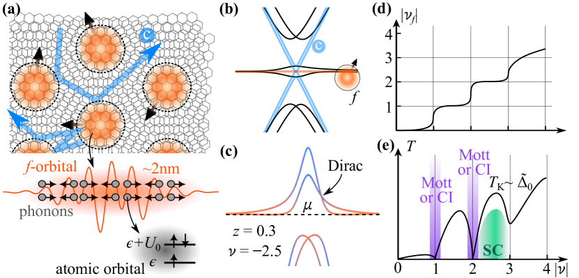
Figure 1: Model. (a) Illustration for the effective $f$- and $c$-electrons. $f$-orbitals are located at AA stacking regions and dominate the flat bands. They are coupled to microscopic phonon modes via the dynamical valley Jahn-Teller effect. (b) Energy bands (black) as a result of hybridization between $f$-bands (orange) and itinerant Dirac $c$-bands (blue). (c) Heavy Fermi liquid bands at $\nu\!=\!-2.5$ with the quasi-particle weight $z\!=\!0.3$. Orange and blue colors represent contributions from $f$- and $c$-electrons, respectively. (d) and (e) sketch the $f$-occupation, $|\nu_{f}|$, and Kondo temperature, $T_{\rm K}$, as functions of the total flat band filling $|\nu|$ in DMFT calculations, respectively.

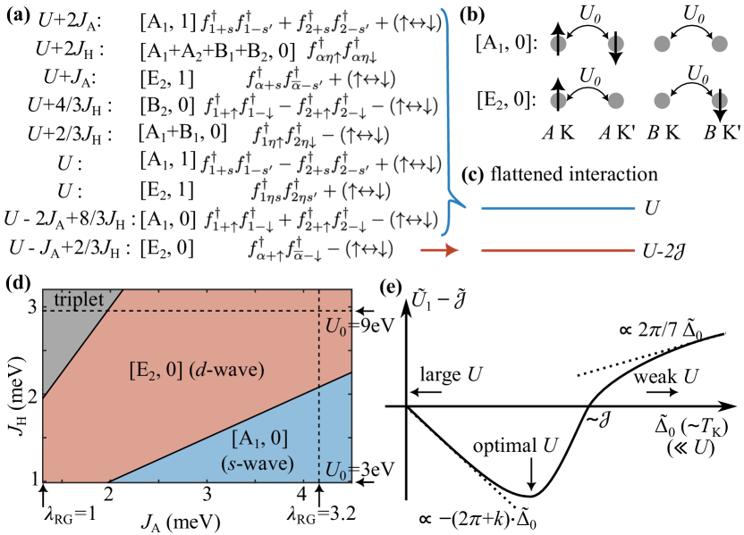
Figure 2: Bare and renormalized interactions. (a) two-electron eigenstates of the interaction Hamiltonian, where the notation $[\rho,j]$ labels the $D_{6}$ representation $\rho$ and total spin $j$. (b) Occupations of graphene sub-lattices ($A,B$) and valleys ($K,K^{\prime}$) of the lowest $E_{2}$ and $A_{1}$ states. (c) The flattened interaction. (d) two-electron ground states in the parameter space of $J_{\rm A}$ and $J_{\rm H}$. All these two-electron states have positive energies due to $U$, hence they cannot form Cooper pairs with the bare interaction. (e) The renormalized interaction $\widetilde{U}_{1}-\widetilde{\mathcal{J}}$ for $d$-wave pairings as a function of the Kondo energy scale $\widetilde{\Delta}_{0}\!\sim\!T_{\rm K}$, which is assumed to be much smaller than the bare repulsion $U$.

Hund’s and anti-Hund’s couplings.

We further consider two additional interactions, $J_{\rm A}$ and $J_{\rm H}$, that originates from electron-phonon couplings and atomic Hubbard repulsion $U_{0}$, respectively. Expressions of these terms are detailed in Appendix A, here we only tabulate their contributions to two-electron states (Fig. 2(a)). The relevant $A_{1}$, $B_{1}$ phonons are in the anti-adiabatic limit because they oscillate much faster than the flat band electrons. Once integrated out, they lead to an inter-valley anti-Hund’s coupling $J_{\rm A}\!=\!\lambda_{\rm RG}\!\times\!1.3$meV Wang et al. (2023), where $\lambda_{\rm RG}\!\approx\!3.2$ is an enhancement factor due to the renormalization effect from higher energy ($\gtrsim 200$meV) states Basko and Aleiner (2008). Among all the two-electron states, $J_{\rm A}$ lowers the energies of inter-valley intra-orbital $s$-wave singlet ($A_{1}$ representation) and inter-valley inter-orbital $d$-wave singlets ($E_{2}$ representation) by $2J_{\rm A}$ and $J_{\rm A}$, respectively.

Hubbard repulsion $U_{0}$ on each carbon atom is usually neglected in theoretical studies of MATBG. As $U_{0}$ is estimated as large as 9eV Wehling et al. (2011), a recent work reported that $U_{0}$ can play an important role in moiré super-lattices Zhang et al. (2022). We find $U_{0}$ leads to an intra-orbital Hund’s coupling $J_{\rm H}\!\approx\!0.33\!\times\!10^{-3}U_{0}$ of the $f$-orbitals. $J_{\rm H}$ tends to forbid the double occupation on each carbon atom as $U_{0}$. Because the $\alpha\!=\!1,2$ $f$-orbitals are mainly distributed on the $A$ and $B$ graphene sub-lattices at the AA stacking site Song and Bernevig (2022), respectively, $J_{\rm H}$ tends to forbid double occupation of each $\alpha$ orbital. Therefore, the inter-orbital $d$-wave states have a smaller energy penalty ($\frac{2}{3}J_{\rm H}$) than that ($\frac{8}{3}J_{\rm H}$) of the intra-orbital $s$-wave state. One can hence expect a $d$-wave ground state stabilized by $J_{\rm H}$. Fig. 2(d) shows a phase diagram of the two-electron ground states in the parameter space of $U_{0}\!=\!3\!\sim\!10$eV and $\lambda_{\rm RG}\!=\!1\!\sim\!3.5$, where the $d$-wave states indeed occupy a large area.

Since both $J_{\rm A}$ and $J_{\rm H}$ are much weaker than $U$, they cannot lead to an attractive bare interaction to stabilize the SC phase. Nevertheless, we find the renormalized interaction can have a pairing potential. To simplify the calculation, we start with the $d$-wave ground states, and introduce a flattened interaction (Fig. 2(c)) such that the ground state energy is set to $U-2\mathcal{J}$ and all excited state energies are set to $U$, where $\mathcal{J}\!\sim\!J_{\rm A}$. The flattened interaction captures main features of the original interaction in that (i) it yields the correct two-electron ground states, and (ii) it is positive definite and does not support any pairing. The corresponding action can be written as (Secs. A.5 and B.1)

$$S_{I}= \frac{1}{2}\int d\tau\sum_{\alpha\eta}\bigg{(}\Big{(}U_{1}+\frac{\mathcal{J}}{2}\Big{)}{N}_{\alpha\eta}{N}_{\overline{\alpha}\overline{\eta}}+U_{2}{N}_{\alpha\eta}{N}_{\alpha\overline{\eta}}$$

$$+U_{3}{N}_{\alpha\eta}{N}_{\overline{\alpha}\eta}+U_{4}{N}_{\alpha\eta}^{2}+2\mathcal{J}\cdot{\bf S}_{\alpha\eta}\cdot{\bf S}_{\overline{\alpha}\overline{\eta}}\bigg{)}\ ,$$ (2)

where $\tau$ is the imaginary time, ${N}_{\alpha\eta}$ and ${\bf S}_{\alpha\eta}$ are respectively the charge and spin operators in the valley $\eta$ and orbital $\alpha$. Here $\overline{\alpha}$ and $\overline{\eta}$ represent the opposite orbital and valley, respectively. The bare parameters are given by $U_{1}\!=\!U\!-\!\mathcal{J}$, $U_{2,3,4}\!=\!U$. An advantage of the flattened interaction is its high symmetry - a $\rm U(1)\!\times\!U(1)\!\times\!U(1)\!\times\!U(1)\!\times\!SU(2)\!\times\!SU(2)$ group generated by $\sigma^{0,z}\tau^{0,z}$ and $(\sigma^{0}\tau^{0}\pm\sigma^{z}\tau^{z})\varsigma^{x,y,z}$, where $\varsigma^{x,y,z}$ are Pauli matrices for the spin degree of freedom. The $C_{3z}\!=\!e^{\frac{2\pi}{3}\sigma^{z}\tau^{z}}$ symmetry is now promoted to a continuous rotation symmetry with the angular momentum $\sigma^{z}\tau^{z}$. The four U(1) symmetries correspond to charge ($\sigma^{0}\tau^{0}$), valley ($\tau^{z}$), orbital ($\sigma^{z}$), and angular momentum ($\sigma^{z}\tau^{z}$) conservations, respectively. The two SU(2) symmetries are independent spin rotations in the $\sigma^{z}\tau^{z}=\pm 1$ flavors, respectively.

As Hund’s and anti-Hund’s couplings. takes the most generic form allowed by the symmetry, the form of $S_{I}$ will remain unchanged under renormalization, but the values of $U_{1,2,3,4}$ and $\mathcal{J}$ can flow. The inter-valley $d$-wave singlet (triplet) states have the energy $U_{1}\!-\!(+)\mathcal{J}$. In the following we show that $U_{1}\!-\!\mathcal{J}$ will flow to a negative value in the heavy Fermi liquid.

Quasi-particles in heavy Fermi liquid.

The ground state of the THF model can be a heavy Fermi liquid (Fig. 1(c)) Chou and Das Sarma (2023); Zhou et al. (2023); Hu et al. (2023a); Lau and Coleman (2023); Datta et al. (2023); Rai et al. (2023). In Fig. 1(e) we sketch the Kondo temperature $T_{\rm K}$ as a function of $\nu$. $T_{\rm K}$ is zero or almost vanishing at $|\nu|=0,1,2$, corresponding to Mott insulators or symmetry-broken CIs Po et al. (2018); Bultinck et al. (2020); Kang and Vafek (2019); Lian et al. (2021); Xie et al. (2021); Liu and Dai (2021); Kennes et al. (2018); Koshino et al. (2018); Xu et al. (2018); Venderbos and Fernandes (2018); Ochi et al. (2018); Seo et al. (2019); Classen et al. (2019); Kang and Vafek (2020); Xie and MacDonald (2020); Cea and Guinea (2020); Zhang et al. (2020); Soejima et al. (2020); Liu et al. (2021b); Da Liao et al. (2021); Hejazi et al. (2021) stabilized by the RKKY interaction. $T_{\rm K}$ becomes non-negligible when the system is doped away from these fillings. As the highest $T_{c}$ of SC is observed at $-3\!<\!\nu\!<\!-2$, in this work we mainly focus on $\nu\!=\!-2-\delta\nu$ with $0\!<\!\delta\nu\!<\!1$. Due to the particle-hole symmetry of the model Song et al. (2021); Bernevig et al. (2021); Song and Bernevig (2022); Wang et al. (2021), physics at $\nu\!=\!2\!+\!\delta\nu$ is the same.

The effective Anderson impurity model is in a local Fermi liquid phase if the lattice model is in a heavy Fermi liquid phase. The local Green’s function at zero temperature consists of a quasi-particle part $z/[i\omega\!-\!\widetilde{\epsilon}_{f}\!+\!i\widetilde{\Delta}_{0}\mathrm{sgn}(\omega)]$ and a featureless incoherent part. Here $z\!=\!(1-\partial_{i\omega}\Sigma(\omega))^{-1}|_{\omega=0}$ is the quasi-particle weight with $\Sigma(\omega)$ denoting the self-energy, $\widetilde{\epsilon}_{f}$ is the renormalized on-site energy, and $\widetilde{\Delta}_{0}\!=\!z\Delta_{0}\!\sim\!T_{\rm K}$ is the renormalized hybridization. The ratio $\widetilde{\epsilon}_{f}/\widetilde{\Delta}_{0}\!=\!\cot\delta_{f}$ is fixed by the occupation of $f$-electrons via the Friedel sum rule, with $\delta_{f}\!=\!\pi(\nu_{f}+4)/8$ being the scattering phase shift. For the considered filling $\nu\!=\!-2\!-\!\delta\nu$, there is $\nu_{f}\!\approx\!-2$, $\delta_{f}\!\approx\!\pi/4$ (Fig. 1(d)). Refs. Zhou et al. (2023); Rai et al. (2023) have shown that $z\!=\!0.2\!\sim\!0.3$ and $\widetilde{\Delta}_{0}\!=\!0.5\!\sim\!1$meV at $\nu\!=\!-2\!-\!\delta\nu$. In the rest of this work we will regard $z$ and $\widetilde{\Delta}_{0}$ as given quantities.

An important quantity for the local Fermi liquid is the (anti-symmetrized) full vertex function $\Gamma_{I_{1},I_{2};I_{3},I_{4}}(\omega_{1},\omega_{2};\omega_{3},\omega_{4})$, defined as the following skeleton diagrams to infinite orders of the bare interaction (denoted as $\Gamma^{0}$)

(3)

Here $I_{i}\!=\!(\alpha_{i},\eta_{i},s_{i})$ is a composite index, and solid lines represent full Green’s functions. Due to the $\rm U(1)^{\times 4}\!\times\!SU(2)^{\times 2}$ symmetry, the zero frequency component $\Gamma(0,0;0,0)$ only has five independent parameters, i.e., $\Gamma_{U1,2,3,4}$ and $\Gamma_{\mathcal{J}}$, which can be understood as the dressed $U_{1,2,3,4}$ and $\mathcal{J}$ for low energy excitations, respectively (Sec. B.2).

It is convenient to define quasi-particle operator $\widetilde{f}\!=\!z^{-\frac{1}{2}}f$. Then the total action $S_{0}\!+\!S_{I}$ can be rewritten as a quasi-particle part $S_{\rm qp}$ plus a counter term $S_{\rm c}$ Hewson (1993a, 2001). $S_{\rm qp}$ has the same form as $S_{0}\!+\!S_{I}$, except that $f$ is replaced by $\widetilde{f}$, $\epsilon_{f}$, ${\Delta}_{0}$ are replaced by the renormalized values $\widetilde{\epsilon}_{f}$, $\widetilde{\Delta}_{0}$, and $U_{1,2,3,4}$, $\mathcal{J}$ are replaced by renormalized interactions $\widetilde{U}_{1,2,3,4}\!=\!z^{2}\Gamma_{U1,2,3,4}$, $\widetilde{\mathcal{J}}\!=\!z^{2}\Gamma_{\mathcal{J}}$ respectively. As parameters in $S_{\rm qp}$ are already fully renormalized physical observables, the counter term $S_{\rm c}$ must cancel further renormalizations at arbitrary order of the renormalized interaction (Sec. B.7).

Renormalized interaction in the $\widetilde{\Delta}_{0}\!\ll\!\mathcal{J}\!\ll\!U$ limit.

In this limit the Kondo temperature $T_{\rm K}\!\sim\!\widetilde{\Delta}_{0}$ defines the single energy scale of the local Fermi liquid Nozières and Blandin (1980); Coleman (2007); Hewson (1993b). Thus, the renormalized interactions $\widetilde{U}_{1,2,3,4}$, $\widetilde{\mathcal{J}}$ can be expressed in terms of $\widetilde{\Delta}_{0}$.

To derive $\widetilde{U}_{1,2,3,4}$, $\widetilde{\mathcal{J}}$, we make use of the Ward identities Yamada (1975a, b); Yoshimori (1976) given by the $\rm U(1)^{\times 4}\!\times\!SU(2)^{\times 2}$ symmetry. Consider a gauge transformation $f_{I}^{\prime}(\tau)\!=\!e^{i\tau\nu O_{I}}f_{I}(\tau)$ for some diagonal symmetry generator $O$. On the one hand, one knows the gauge transformed Green’s function $\mathcal{G}^{\prime}$ and can calculate $\mathcal{G}^{\prime}-\mathcal{G}$ to first order of $\nu$. On the other hand, one can rewrite $S[f^{\dagger},f]$ in terms of $S[f^{\prime\dagger},f^{\prime}]$ plus a perturbation $\Delta S[f^{\prime\dagger},f^{\prime}]$, which is a bilinear term in the fermion field. The leading order correction $\delta\mathcal{G}$ due to $\Delta S$ is given by a skeleton diagram involving the full vertex $\Gamma$ Landau and Lifshitz (2013). Equaling $\mathcal{G}^{\prime}-\mathcal{G}$ and $\delta\mathcal{G}$, one obtains the Ward identity at zero temperature (Sec. B.4)

$$\frac{\partial\Sigma(\omega_{1})}{\partial i\omega_{1}}\sum_{I_{1}}O_{I_{1}}^{2}=\sum_{I_{1}}\frac{\partial\Sigma_{I_{1}}(\omega_{1})}{\partial h}O_{I_{1}}$$

$$-\frac{\sin^{2}(\delta_{f})}{\pi\Delta_{0}}\sum_{I_{1}I_{2}}\Gamma_{I_{1}I_{2};I_{2}I_{1}}(\omega_{1},0;0,\omega_{1})\cdot O_{I_{1}}O_{I_{2}}\ .$$ (4)

Here $\partial_{h}\Sigma$ is the response of self-energy to an external field $\!-h\sum_{I}f^{\dagger}_{I}O_{I}f_{I}$. It is further related to the exact static susceptibility $\chi^{O}\!=\!\frac{\sin^{2}(\delta_{f})}{\pi\Delta_{0}}\sum_{I}(O_{I}^{2}-\partial_{h}\Sigma_{I}(0)O_{I})$ of the operator $O$.

Setting $\omega_{1}\!=\!0$, Renormalized interaction in the $\widetilde{\Delta}_{0}\!\ll\!\mathcal{J}\!\ll\!U$ limit. relates $\Gamma(0,0;0,0)$, which defines the renormalized interactions, to quasi-particle weight ($\partial_{i\omega}\Sigma\!=\!1\!-\!z^{-1}$) and exact susceptibilities ($\partial_{h}\Sigma$). We find charge $\sigma^{0}\tau^{0}\varsigma^{0}$ ($l=c$), spin $\varsigma^{z}$ ($s$), valley $\tau^{z}$ ($v$), and orbital $\sigma^{z}$ ($o$) susceptibilities can be expressed in terms of $\widetilde{\Delta}_{0}$ and renormalized interactions as $\chi^{l}\!=\!\frac{4}{\pi\widetilde{\Delta}_{0}}(1-\frac{1}{2\pi\widetilde{\Delta}_{0}}\widetilde{A}^{l})$, $\widetilde{A}^{c}\!=\!2\widetilde{U}_{1}+2\widetilde{U}_{2}+2\widetilde{U}_{3}+\widetilde{U}_{4}+\widetilde{\mathcal{J}}$, $\widetilde{A}^{s}\!=\!-\widetilde{U_{4}}+\widetilde{\mathcal{J}}$, $\widetilde{A}^{v}\!=\!-2\widetilde{U}_{1}-2\widetilde{U}_{2}+2\widetilde{U}_{3}+\widetilde{U}_{4}-\widetilde{\mathcal{J}}$, $\widetilde{A}^{o}\!=\!-2\widetilde{U}_{1}+2\widetilde{U}_{2}-2\widetilde{U}_{3}+\widetilde{U}_{4}-\widetilde{\mathcal{J}}$. Since $\widetilde{\Delta}_{0}\!\ll\!\mathcal{J}$ and $\nu_{f}\!\approx\!-2$, only the two-electron ground states, i.e., the inter-valley $d$-wave singlets (Fig. 2(a)), will participate in the Kondo screening Nozières and Blandin (1980). As charge, spin, valley, and orbital operators are constants in the ground states, the corresponding susceptibilities are not contributed by the quasi-particles Hewson (1993a, b); Nishikawa et al. (2010). Therefore, $\chi^{c,s,v,o}$ will not diverge as the quasi-particle density of states ($\sim\!\widetilde{\Delta}_{0}^{-1}$) in the $\widetilde{\Delta}_{0}\!\to\!0$ limit, which indicates the universal behaviors

$$\widetilde{U}_{1}=-2\pi\widetilde{\Delta}_{0},\quad\widetilde{U}_{2,3}=2\pi\widetilde{\Delta}_{0}-\frac{\widetilde{\mathcal{J}}}{2},\quad\widetilde{U}_{4}=-2\pi\widetilde{\Delta}_{0}+\widetilde{\mathcal{J}}\ .$$ (5)

One of the two-electron eigenvalues of the renormalized interaction, $\widetilde{U}_{1}\mp\widetilde{\mathcal{J}}$ (given after Hund’s and anti-Hund’s couplings.), must be negative. Therefore, we have proven that the renormalized interaction must possess a pairing channel at $\nu_{f}\!\approx\!-2$ in the $\widetilde{\Delta}_{0}\!\ll\!\mathcal{J}$ limit. Susceptibilities of other quantities suggest $\widetilde{\mathcal{J}}=k\widetilde{\Delta}_{0}$ with $k$ being a universal constant that ranges from 4.6 to 10.3 (Sec. B.6). A positive $\widetilde{\mathcal{J}}$ favors the inter-valley $d$-wave singlet pairing.

Renormalized interaction in the $\mathcal{J}\!\ll\!\widetilde{\Delta}_{0}\!\ll\!U$ limit.

$\mathcal{J}$ plays a minor role in the local Fermi liquid if it is much smaller than the Kondo temperature Nozières and Blandin (1980). As $S_{I}$ has a U(8) symmetry in the absence of $\widetilde{\mathcal{J}}$, $U_{1,2,3,4}$ will remain equal under the renormalization. Freezing the charge susceptibility fixes $\widetilde{U}_{1,2,3,4}\!=\!\frac{2\pi}{7}\widetilde{\Delta}_{0}$ Nishikawa et al. (2010).

Fig. 2(e) shows the renormalized pairing potential $\widetilde{U}_{1}\!-\!\widetilde{\mathcal{J}}$ as a function of $\widetilde{\Delta}_{0}$. The $\widetilde{\Delta}_{0}\!\ll\!\mathcal{J}$ and $\mathcal{J}\!\ll\!\widetilde{\Delta}_{0}$ limits exhibit universal behaviors that are soley determined by the $\rm U(1)^{\times 4}\!\times\!SU(2)^{\times 2}$ and U(8) symmetries, respectively. The intermediate regime ($\widetilde{\Delta}_{0}\!\sim\!\mathcal{J}$) loses the universality, and one can expect a transition of the sign of $\widetilde{U}_{1}\!-\!\widetilde{\mathcal{J}}$. The non-monotonous dependence of $\widetilde{U}_{1}\!-\!\widetilde{\mathcal{J}}$ on $\widetilde{\Delta}_{0}$ suggests an optimal $\widetilde{\Delta}_{0}$ for SC. As $\widetilde{\Delta}_{0}$ monotonously decreases with $U$, this also suggests the existence of an optimal $U$.

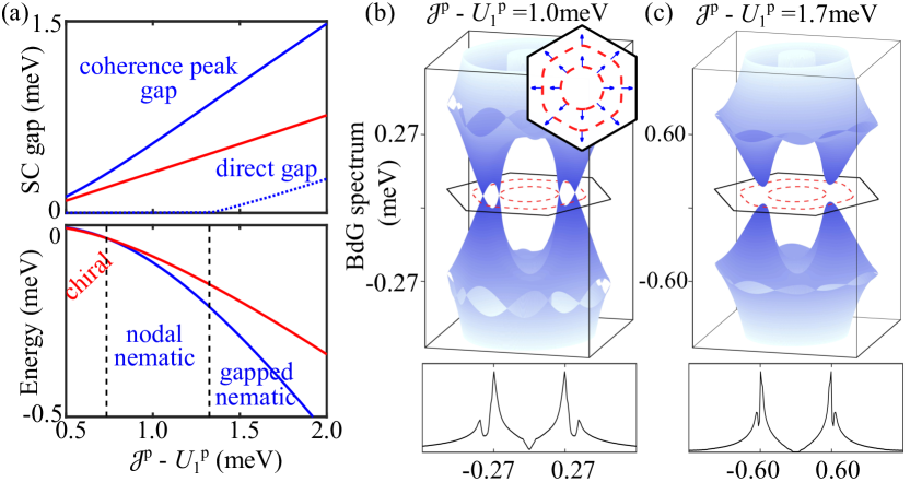
Figure 3: Mean-field calculations of SC at $\nu\!=\!-\!2.5$ and $z=0.3$. (a) Phase diagram of inter-valley inter-orbital $d$-wave singlet SC. The range of $\mathcal{J}^{\rm p}\!-\!U_{1}^{\rm p}$ corresponds to $T_{\rm K}$ ranging from 1.7K to 7.1K if $k\!=\!8$. (b) BdG bands of the nematic $d$-wave SC with a $p$-wave-like nodal structure. The inset shows the $C_{2z}T$ sewing matrix phase $\phi_{\mathbf{k}}$ on the Fermi surface. (c) BdG bands of the gapped nematic $d$-wave SC, where the gap function is still highly anisotropic. The lower panels in (b) and (c) are the corresponding densities of states calculated using a Lorentz spread 0.004meV.

Quasi-particle mean-field theory.

We now investigate SC on the moiré lattice using a renormalized THF model. Its free part is

$${\epsilon}_{f}\sum_{\mathbf{k}}\widetilde{f}_{\mathbf{k}}^{\dagger}\widetilde{f}_{\mathbf{k}}+c_{\mathbf{k}}^{\dagger}\mathcal{H}^{(c)}(\mathbf{k})c_{\mathbf{k}}+z^{\frac{1}{2}}\left[c_{\mathbf{k}}^{\dagger}\mathcal{H}^{(cf)}(\mathbf{k})\widetilde{f}_{\mathbf{k}}+h.c.\right].$$ (6)

$\widetilde{f}_{\mathbf{k}}$ ($c_{\mathbf{k}}$) is a column vector of annihilation operators for $f$-quasi-particle ($c$-electron) in different flavors, i.e., valley, orbital, spin, etc., at momentum $\mathbf{k}$, $\epsilon_{f}$ is a lagrangian multiplier introduced to fix $\nu_{f}\!\approx\!-2$, $\mathcal{H}^{(c)}$ and $\mathcal{H}^{(cf)}$ are coupling matrices descending from the THF model (Appendix C). The renormalized $cf$ hybridization is suppressed by $z^{\frac{1}{2}}$ Zhou et al. (2023). In a mean-field calculation, the effective local interaction should be defined by $z^{2}\Gamma^{\rm p}$ instead of $z^{2}\Gamma$ to avoid over counting Georges et al. (1996), where $\Gamma^{\rm p}$ is the irreducible vertex represented by diagrams in Eq. 3 that cannot be split by cutting two lines going left. $z^{2}\Gamma^{\rm p}$ has the same pairing channel (inter-valley $d$-wave singlet) as $z^{2}\Gamma$ but with a weaker potential (Secs. B.5 and B.6)

$$U_{1}^{\rm p}-\mathcal{J}^{\rm p}=\frac{\widetilde{U}_{1}-\widetilde{\mathcal{J}}}{1-\frac{1}{4\widetilde{\Delta}_{0}}(\widetilde{U}_{1}-\widetilde{\mathcal{J}})}=-\frac{(2\pi+k)}{1+\frac{2\pi+k}{4}}\widetilde{\Delta}_{0}$$ (7)

in the $\widetilde{\Delta}_{0}\ll\mathcal{J}$ limit.

We carry out mean-field calculations for the SC at $\nu\!=\!-2.5$ using $z\!=\!0.3$ and $\mathcal{J}^{\rm p}\!-\!U_{1}^{\rm p}$ in the range from 0.5 to 2meV (Fig. 3). Since the $d$-wave pairings form the two-dimensional representation $E_{2}$, we find two possible SC phases. The first is a chiral $d$-wave pairing $\widetilde{f}_{\mathbf{k}\alpha+\uparrow}^{\dagger}\widetilde{f}_{-\mathbf{k}\overline{\alpha}-\downarrow}^{\dagger}\!-\!(\uparrow\leftrightarrow\downarrow)$ (for either $\alpha$=1 or 2) that breaks $C_{2x}$, $C_{2y}$, and time-reversal symmetries. It is always gapped. The second is a nematic $d$-wave pairing Wu et al. (2018); Liu et al. (2023); Blason and Fabrizio (2022) $e^{-i\varphi}\widetilde{f}_{\mathbf{k}1+\uparrow}^{\dagger}\widetilde{f}_{-\mathbf{k}2-\downarrow}^{\dagger}\!+\!e^{i\varphi}\widetilde{f}_{\mathbf{k}2+\uparrow}^{\dagger}\widetilde{f}_{-\mathbf{k}1-\downarrow}^{\dagger}\!-\!(\uparrow\leftrightarrow\downarrow)$ that breaks the $C_{3z}$ symmetry. Here $\varphi$ sets the orientation of the nematic order. We find the nematic phase can be either nodal or gapped. When $\mathcal{J}^{\rm p}\!-\!U_{1}^{\rm p}<$0.7meV, the chiral state has a slightly lower energy than the nematic state. When $\mathcal{J}^{\rm p}\!-\!U_{1}^{\rm p}>$0.7meV, the nematic state has a significantly lower energy than the chiral state.

$p$-wave-like nodal SC.

An intermediate pairing strength (Fig. 3(a)) leads to a $p$-wave-like nodal structure, as shown in Fig. 3(b). We now prove that the 2 (mod 4) nodes on each Fermi surface (FS) are guaranteed by the $\pi$ Berry’s phase protected by $C_{2z}T$ symmetry. Suppose $\psi_{\mathbf{k}+s}$ is the annihilation operator for Bloch states on a given FS in the $\eta\!=\!+$ valley, and $(C_{2z}T)\psi_{\mathbf{k}+s}^{\dagger}(C_{2z}T)^{-1}\!=\!\psi_{\mathbf{k}+s}^{\dagger}e^{i\phi_{\mathbf{k}}}$. Due to $(C_{2z}T)\widetilde{f}_{\mathbf{k}\alpha\eta s}^{\dagger}(C_{2z}T)^{-1}\!=\!\widetilde{f}_{\mathbf{k}\overline{\alpha}\eta s}^{\dagger}$, there must be $\psi^{\dagger}_{\mathbf{k}+s}\sim\widetilde{f}^{\dagger}_{\mathbf{k}1+s}+e^{-i\phi_{\mathbf{k}}}\widetilde{f}^{\dagger}_{\mathbf{k}2+s}$. Bloch states in the $\eta\!=\!-$ valley can be obtained by applying the time-reversal: $\psi^{\dagger}_{-\mathbf{k}-s}\!\sim\!\widetilde{f}^{\dagger}_{-\mathbf{k}1-s}\!+e^{i\phi_{\mathbf{k}}}\widetilde{f}^{\dagger}_{-\mathbf{k}2-s}$. Projecting the nematic $d$-wave pairing onto the FS, we obtain $\cos(\phi_{\mathbf{k}}+\varphi)\cdot\psi_{\mathbf{k}+\uparrow}^{\dagger}\psi_{-\mathbf{k}-\downarrow}^{\dagger}-(\uparrow\leftrightarrow\downarrow)$. As the FS encloses an odd number of Dirac points (Fig. 1(c)), $\phi_{\mathbf{k}}$ must wind an odd ($2n\!+\!1$) multiple of $2\pi$ along the FS (Fig. 3(b)) Ahn et al. (2019), leaving $4n+2$ nodes at $\phi_{\mathbf{k}}+\varphi=\pm\frac{\pi}{2}$.

An alternative understanding of the pairing nodes is the Euler obstruction Yu et al. (2022), which states that a $C_{2z}T$-symmetric pairing diagonal in the Chern basis must have zeros in the Brillouin zone if the Euler class Ahn et al. (2019) of the normal state bands is nontrivial, as it is MATBG. Since $f_{\alpha\eta s}$ has a large overlap with the $C\!=\!(-1)^{\alpha}\eta$ Chern basis Song and Bernevig (2022), the nematic $d$-wave pairing has a large component (more than $95\%$) in the obstructed channel.

As the pairing becomes stronger, nodes on the two FSs will merge eventually, leading to a gapped phase (Fig. 3(c)). Spectrum of the gapped nematic SC remains highly anisotropic if the direct gap, opened by merging Dirac nodes, is significantly smaller than the pairing. Therefore, both the nodal and the gapped nematic $d$-wave SC can have a V-shaped density of states at an energy scale larger than the direct gap (0 in the nodal case). This is consistent with the V-shaped spectrum Oh et al. (2021) and nematicity Cao et al. (2021) seen in experiments.

Discussion.

Our theory also brings insights into strong coupling features of the SC in MATBG. The pairing potential $\mathcal{J}^{\rm p}\!-\!U_{1}^{\rm p}$ (Eq. 7) is a few times of $T_{\rm K}$, and the Fermi energy $E_{F}$ is of the same order of $T_{\rm K}$ (Fig. 1(c)). Therefore, $\mathcal{J}^{\rm p}\!-\!U_{1}^{\rm p}\gtrsim E_{F}$, and the SC is closer to a BEC state than a BCS state Cao et al. (2018a). The pairing is mainly localized at “moiré molecules” in AA-stacking regions and hence has a much smaller phase stiffness compared to conventional BCS pairings of delocalized Xie et al. (2020) states. This may explain the large ratio between pairing gap and $T_{c}$ Oh et al. (2021).

Appendix A Local interaction

A.1 Local (moiré) orbitals

Here we summarize the relevant local interactions in a single AA-stacking region of magic-angle twisted bilayer graphene (MATBG). There are eight effective local $f$-orbitals in an AA-stacking region Song and Bernevig (2022): $f_{\alpha,\eta,s}$, where $\alpha=1,2$ is the orbital index, $\eta=\pm$ is the valley index, and $s=\uparrow,\downarrow$ is the spin index. A single AA-site has the time-reversal symmetry ($T$) and symmetries of the $D_{6}$ point group. The single-particle representations of these discrete symmetries are given in section S2A of the supplementary material of Ref. Song and Bernevig (2022). They are

$$T=\sigma^{0}\tau^{x}\varsigma^{0}K,\qquad C_{2z}=\sigma^{x}\tau^{x}\varsigma^{0},\qquad C_{3z}=e^{i\frac{2\pi}{3}\sigma^{z}\tau^{z}\varsigma^{0}},\qquad C_{2x}=\sigma^{x}\tau^{0}\varsigma^{0}\ ,$$ (8)

where $K$ is the complex conjugation. Their actions on the second quantized operators can be obtained directly

$$Tf_{\alpha\eta s}^{\dagger}T^{-1}=f^{\dagger}_{\alpha\overline{\eta}s},\qquad C_{2z}f_{\alpha\eta s}^{\dagger}C_{2z}^{-1}=f_{\overline{\alpha}\overline{\eta}s}^{\dagger},\qquad C_{3z}f_{\alpha\eta s}^{\dagger}C_{3z}^{-1}=e^{i\frac{2\pi}{3}\eta(-1)^{\alpha-1}}f_{\alpha\eta s}^{\dagger},\qquad C_{2x}f_{\alpha\eta s}^{\dagger}C_{2x}^{-1}=f^{\dagger}_{\overline{\alpha}\eta s}\ .$$ (9)

In this work we do not distinguish the single-particle and the second-quantized representations of symmetry operators. If we write a unitary (anti-unitary) symmetry operator $g$ as a matrix $D^{g}$ ($D^{g}\cdot K$), as exampled in Eq. 8, then its action on second-quantized operators is defined by

$$gf^{\dagger}_{\alpha\eta s}g^{-1}=\sum_{\alpha^{\prime}\eta^{\prime}s^{\prime}}D_{\alpha^{\prime}\eta^{\prime}s^{\prime},\alpha\eta s}^{g}f_{\alpha^{\prime}\eta^{\prime}s^{\prime}}^{\dagger},\qquad gf_{\alpha\eta s}g^{-1}=\sum_{\alpha^{\prime}\eta^{\prime}s^{\prime}}D_{\alpha^{\prime}\eta^{\prime}s^{\prime},\alpha\eta s}^{g*}f_{\alpha^{\prime}\eta^{\prime}s^{\prime}}\ .$$ (10)

We denote the fermion creation operator of the $p_{z}$ orbital at the carbon atom belonging to the layer $l$ (=$+$ for the top layer and $-$ for the bottom layer) by $c_{l\mathbf{r}s}^{\dagger}$. Here $s$ is the spin index, $\mathbf{r}\in\mathcal{L}_{l,1}+\mathcal{L}_{l,2}$ is the position of the atom, and $\mathcal{L}_{l,\beta}$ is the $\beta$-sub-lattice of the layer $l$, where we associate the A-, B-sub-lattices of graphene to $\beta=1$ and 2, respectively. Projected $c_{l\mathbf{r}s}^{\dagger}$ can be written in terms of the $f$ operators as

$$\psi_{l\mathbf{r}s}^{\dagger}=\sqrt{\Omega_{\rm G}}\sum_{\eta\alpha}\sum_{\beta,\mathcal{L}_{l,\beta}\ni\mathbf{r}}e^{-i\eta\mathbf{K}_{l}\cdot\mathbf{r}}w_{l\beta,\alpha}^{(\eta)*}(\mathbf{r})f_{\alpha\eta s}^{\dagger}\ .$$ (11)

Here $\pm\mathbf{K}_{l}$ are the momenta of Dirac points in the layer $l$, $\mathbf{K}_{+}=\frac{4\pi}{3a_{\rm G}}(\cos\frac{\theta}{2},\sin\frac{\theta}{2})$, $\mathbf{K}_{-}=\frac{4\pi}{3a_{\rm G}}(\cos\frac{\theta}{2},-\sin\frac{\theta}{2})$, with $a_{\rm G}=2.46\mathring{\rm A}$ being the graphene lattice constant and $\theta\approx 1.08^{\circ}$ the magic twist angle. The length of $\mathbf{K}_{l}$ is given by $|\mathbf{K}_{l}|=\frac{4\pi}{3a_{\rm G}}\approx 1.703\mathring{\rm A}^{-1}$. $\Omega_{\rm G}=\frac{\sqrt{3}}{2}a_{\rm G}^{2}$ is the area of a graphene unit cell. $w_{l\beta,\alpha}^{(\eta)}(\mathbf{r})$ is the localized Wannier functions constructed in Ref. Song and Bernevig (2022). The summation over the sub-lattice index $\beta$ on the right hand side is limited to the one containing $\mathbf{r}$ on the left hand side, i.e., $\mathcal{L}_{l,\beta}\ni\mathbf{r}$. Section S2A of the supplementary material of Ref. Song and Bernevig (2022) provides a Gaussian approximation for the Wannier functions:

$$w_{l1,1}^{(\eta)}(\mathbf{r})=\frac{\alpha_{1}}{\sqrt{2}}\frac{1}{\sqrt{\pi\lambda_{1}^{2}}}e^{i\frac{\pi}{4}l\eta-\mathbf{r}^{2}/(2\lambda_{1}^{2})},\quad w_{l2,1}^{(\eta)}(\mathbf{r})=-l\frac{\alpha_{2}}{\sqrt{2}}\frac{x+i\eta y}{\lambda_{2}^{2}\sqrt{\pi}}e^{i\frac{\pi}{4}l\eta-\mathbf{r}^{2}/(2\lambda_{2}^{2})},$$ (12)

$$w_{l1,2}^{(\eta)}(\mathbf{r})=l\frac{\alpha_{2}}{\sqrt{2}}\frac{x-i\eta y}{\lambda_{2}^{2}\sqrt{\pi}}e^{-i\frac{\pi}{4}l\eta-\mathbf{r}^{2}/(2\lambda_{2}^{2})},\qquad w_{l2,2}^{(\eta)}(\mathbf{r})=\frac{\alpha_{1}}{\sqrt{2}}\frac{1}{\sqrt{\pi\lambda_{1}^{2}}}e^{-i\frac{\pi}{4}l\eta-\mathbf{r}^{2}/(2\lambda_{1}^{2})}\ .$$ (13)

At the magic-angle, the parameters are estimated as

$$\alpha_{1}=0.8193,\qquad\alpha_{2}=0.5734,\qquad\lambda_{1}=0.1791a_{\rm M},\qquad\lambda_{2}=0.1910a_{\rm M}\ .$$ (14)

where $a_{\rm M}=\frac{4\pi}{3k_{\theta}}=\frac{a_{\rm G}}{2\sin\frac{\theta}{2}}\approx 54.57a_{\rm G}\approx 134.2\mathring{\rm A}$ is the moiré lattice constant.

A.2 Coulomb interaction and intra-orbital Hund’s coupling

The widely studied Coulomb interaction in MATBG is

$$H_{I1}=\frac{1}{2}\sum_{\eta\eta^{\prime}}\sum_{\mathbf{r}}\sum_{\mathbf{r}^{\prime}}V(\mathbf{r}-\mathbf{r}^{\prime})\left[\rho^{(\eta\eta)}(\mathbf{r})\rho^{(\eta^{\prime}\eta^{\prime})}(\mathbf{r}^{\prime})+\rho^{(\eta\overline{\eta})}(\mathbf{r})\rho^{(\overline{\eta}\eta^{\prime})}(\mathbf{r}^{\prime})\right]\ ,$$ (15)

where

$$\rho^{(\eta\eta^{\prime})}(\mathbf{r})= \Omega_{\rm G}\sum_{\alpha\alpha^{\prime}s}\sum_{l}\sum_{\beta,\mathcal{L}_{l\beta}\ni\mathbf{r}}e^{-i(\eta\mathbf{K}_{l}-\eta^{\prime}\mathbf{K}_{l})\cdot\mathbf{r}}w_{l\beta,\alpha}^{(\eta)*}(\mathbf{r})w_{l\beta,\alpha^{\prime}}^{(\eta^{\prime})}(\mathbf{r})f_{\alpha\eta s}^{\dagger}f_{\alpha^{\prime}\eta^{\prime}s}$$ (16)

and

$$V(\mathbf{r})=U_{\xi}\sum_{n=-\infty}^{\infty}\frac{(-1)^{n}}{\sqrt{(\mathbf{r}/\xi)^{2}+n^{2}}}$$ (17)

is the double-gate-screened Coulomb interaction. Here $\xi$ is the distance between the two gates, $U_{\xi}=e^{2}/(4\pi\epsilon\xi)$, and $\epsilon\approx 6$ is the dielectric constant. For $\xi=10$nm, there is $U_{\xi}=24$meV. This interaction respects a valley-U(1) symmetry. Bilinear terms due to the normal order form of operators are omitted because they can be absorbed into the chemical potential for the single-site problem. The Fourier transformation of $V(\mathbf{r})$ is

$$V(\mathbf{r})=\int\frac{d^{2}\mathbf{q}}{(2\pi)^{2}}V(\mathbf{q})e^{-i\mathbf{q}\cdot\mathbf{r}},\qquad V(\mathbf{q})=\pi\xi^{2}U_{\xi}\frac{\tanh(\xi|\mathbf{q}|/2)}{\xi|\mathbf{q}|/2}\ .$$ (18)

The projected intra-valley scattering interaction between $\rho^{(\eta\eta)}$ and $\rho^{(\eta^{\prime}\eta^{\prime})}$ has been calculated in section S3B of the supplementary material of Ref. Song and Bernevig (2022). It has the form

$$H_{I1}=\frac{U}{2}\sum_{\alpha\eta s}\sum_{\alpha^{\prime}\eta^{\prime}s^{\prime}}f_{\alpha\eta s}^{\dagger}f_{\alpha^{\prime}\eta^{\prime}s^{\prime}}^{\dagger}f_{\alpha^{\prime}\eta^{\prime}s^{\prime}}f_{\alpha\eta s}=U\frac{\hat{N}(\hat{N}-1)}{2},\qquad U\approx 58\mathrm{meV}\ ,$$ (19)

where $\hat{N}$ is the particle number operator. There is no other term, e.g., Hund’s coupling, contributed by the intra-valley scattering due to the symmetry of MATBG. One can see discussions around Eq. (S135) of the supplementary material of Ref. Song and Bernevig (2022) for the proof.

Now we consider the inter-valley scattering interaction between $\rho^{(\eta\overline{\eta})}$ and $\rho^{(\overline{\eta}\eta)}$. Due to the large momentum transfer $\sim 2\mathbf{K}_{l}$, this interaction is strongly suppressed and usually neglected. Here we discuss it in more details. The relevant Fourier component for this interaction is $V(\pm 2\mathbf{K}_{l}+\mathbf{q})\approx V(\pm 2\mathbf{K}_{l})=\frac{\pi\xi U_{\xi}}{|\mathbf{K}_{l}|}\approx 4.4\times 10^{3}\mathrm{meV\!\cdot\!\mathring{A}^{2}}$. As $V(\pm 2\mathbf{K}_{l}+\mathbf{q})$ is almost $\mathbf{q}$-independent, it gives a $\delta$-like interaction on the microscopic graphene lattice. The projected interaction on the moiré orbitals can be estimated as $\frac{4427\mathrm{meV\cdot\mathring{A}^{2}}}{\Omega_{\rm M}}\approx 0.3$meV, with $\Omega_{\rm M}=\frac{\sqrt{3}}{2}a_{\rm M}^{2}\approx 1.560\times 10^{4}\mathring{\rm A}^{2}$ being the moiré unit cell area. Therefore, this inter-valley scattering interaction contributed by $V(\mathbf{r})$ is indeed much weaker compared to the intra-valley one.

Another usually omitted Coulomb interaction is the on-site Hubbard repulsion $U_{0}$ of the $p_{z}$ orbital of carbon atom. $U_{0}$ is estimated as large as 9.3eV Wehling et al. (2011), which, however, is still smaller than the critical values for the spin-liquid phase ($3.5t$) and anti-ferromagnetic phase ($(4.5\pm 0.5)t$) of graphene as the hopping $t\approx 2.8$eV is also large. Recently, Ref. Zhang et al. (2022) reported that $U_{0}$ plays an important role in the correlated ground state of twisted multilayer graphene systems. We find that $U_{0}$ leads to a non-negligible Hund’s coupling in MATBG. The microscopic interaction is

$$H_{I2}=\frac{U_{0}}{2}\sum_{lss^{\prime}}\sum_{\mathbf{r}}\psi_{l\mathbf{r}s}^{\dagger}\psi_{l\mathbf{r}s^{\prime}}^{\dagger}\psi_{l\mathbf{r}s^{\prime}}\psi_{l\mathbf{r}s}\ .$$ (20)

Projecting it onto the $f$-orbitals, we obtain

$$H_{I2}= \frac{U_{0}\Omega_{\rm G}^{2}}{2}\sum_{l\beta}\sum_{\mathbf{r}\in\mathcal{L}_{l\beta}}\sum_{\alpha_{1,2,3,4}}\sum_{\eta_{1,2,3,4}}\delta_{\eta_{1}+\eta_{2},\eta_{3}+\eta_{4}}w_{l\beta,\alpha_{1}}^{(\eta_{1})*}(\mathbf{r})w_{l\beta,\alpha_{2}}^{(\eta_{2})*}(\mathbf{r})w_{l\beta,\alpha_{3}}^{(\eta_{3})}(\mathbf{r})w_{l\beta,\alpha_{4}}^{(\eta_{4})}(\mathbf{r})f_{\alpha_{1}\eta_{1}s}^{\dagger}f_{\alpha_{2}\eta_{2}s^{\prime}}^{\dagger}f_{\alpha_{3}\eta_{3}s^{\prime}}f_{\alpha_{4}\eta_{4}s}$$

$$= \frac{U_{0}\Omega_{\rm G}}{2}\sum_{l\beta}\sum_{\alpha_{1,2,3,4}}\sum_{\eta_{1,2,3,4}}\delta_{\eta_{1}+\eta_{2},\eta_{3}+\eta_{4}}f_{\alpha_{1}\eta_{1}s}^{\dagger}f_{\alpha_{2}\eta_{2}s^{\prime}}^{\dagger}f_{\alpha_{3}\eta_{3}s^{\prime}}f_{\alpha_{4}\eta_{4}s}\int d^{2}\mathbf{r}\ w_{l\beta,\alpha_{1}}^{(\eta_{1})*}(\mathbf{r})w_{l\beta,\alpha_{2}}^{(\eta_{2})*}(\mathbf{r})w_{l\beta,\alpha_{3}}^{(\eta_{3})}(\mathbf{r})w_{l\beta,\alpha_{4}}^{(\eta_{4})}(\mathbf{r})\ .$$ (21)

Notice that $U_{0}\Omega_{\rm G}\approx 4.7\times 10^{4}\mathrm{meV\!\cdot\!\mathring{A}^{2}}$ ($U_{0}$ taken as 9eV) is one order larger than $V(\pm\mathbf{K}_{l})$. As the Wannier functions have the $C_{3z}$ eigenvalue $e^{i\frac{2\pi}{3}\eta(-1)^{\alpha-1}}$, quasi-angular momentum conservation gives the constraint

$$\eta_{1}(-1)^{\alpha_{1}-1}+\eta_{2}(-1)^{\alpha_{2}-1}=\eta_{3}(-1)^{\alpha_{3}-1}+\eta_{4}(-1)^{\alpha_{4}-1}\mod 3\ .$$ (22)

Using the Gaussian wave-functions in Eqs. 12 and 13 and the valley-U(1), $C_{3z}$ symmetries, we find there are only two types of matrix elements in $H_{I2}$. We summarize them in the following table

$$\begin{tabular}[]{c|c|c|c|c|c}&$\alpha_{1}$&$\alpha_{2}$&$\alpha_{3}$&$\alpha_{4}$&$\eta$'s\\ \hline\cr$J_{\rm H}$&$\alpha_{1}$&$\alpha_{1}$&$\alpha_{1}$&$\alpha_{1}$&$\eta_{1}+\eta_{2}=\eta_{3}+\eta_{4}$\\ \hline\cr$J_{\rm H}^{\prime}$&$\alpha_{1}$&$\alpha_{1}$&$\overline{\alpha}_{1}$&$\overline{\alpha}_{1}$&$\eta_{1}=\overline{\eta}_{2}$, $\eta_{3}=\overline{\eta}_{4}$\\ \hline\cr$J_{\rm H}^{\prime}$&$\alpha_{1}$&$\overline{\alpha}_{1}$&$\overline{\alpha}_{1}$&$\alpha_{1}$&$\eta_{1}=\eta_{4}$, $\eta_{2}=\eta_{3}$\\ \hline\cr$J_{\rm H}^{\prime}$&$\alpha_{1}$&$\overline{\alpha}_{1}$&$\alpha_{1}$&$\overline{\alpha}_{1}$&$\eta_{1}=\eta_{3}$, $\eta_{2}=\eta_{4}$\end{tabular}\ .$$ (23)

The two parameters are

$$J_{\rm H}= U_{0}\Omega_{\rm G}\sum_{l\beta}\int d^{2}\mathbf{r}|w_{l\beta,\alpha_{1}}^{(\eta_{1})}(\mathbf{r})|^{2}|w_{l\beta,\alpha_{1}}^{(\eta_{2})}(\mathbf{r})|^{2}=2U_{0}\Omega_{\rm G}\int d^{2}\mathbf{r}\left[\left(\frac{\alpha_{1}^{2}}{2\pi\lambda_{1}^{2}}\right)^{2}e^{-2\frac{\mathbf{r}^{2}}{\lambda_{1}^{2}}}+\left(\frac{\alpha_{2}^{2}}{2\pi\lambda_{2}^{4}}\right)^{2}\mathbf{r}^{4}e^{-2\frac{\mathbf{r}^{2}}{\lambda_{2}^{2}}}\right]$$

$$= U_{0}\Omega_{\rm G}\left[\frac{\alpha_{1}^{4}}{4\pi\lambda_{1}^{2}}+\frac{\alpha_{2}^{4}}{8\pi\lambda_{2}^{2}}\right]\ ,$$ (24)

$$J_{\rm H}^{\prime}= U_{0}\Omega_{\rm G}\sum_{l\beta}\int d^{2}\mathbf{r}|w_{l\beta,\alpha_{1}}^{(\eta_{1})}(\mathbf{r})|^{2}|w_{l\beta,\overline{\alpha}_{1}}^{(\eta_{3})}(\mathbf{r})|^{2}=4U_{0}\Omega_{\rm G}\int d^{2}\mathbf{r}\left[\left(\frac{\alpha_{1}^{2}}{2\pi\lambda_{1}^{2}}\right)e^{-\frac{\mathbf{r}^{2}}{\lambda_{1}^{2}}}\times\left(\frac{\alpha_{2}^{2}}{2\pi\lambda_{2}^{4}}\right)\mathbf{r}^{2}e^{-\frac{\mathbf{r}^{2}}{\lambda_{2}^{2}}}\right]$$

$$= U_{0}\Omega_{\rm G}\frac{\alpha_{1}^{2}\alpha_{2}^{2}\lambda_{1}^{2}}{\pi(\lambda_{1}^{2}+\lambda_{2}^{2})^{2}}\ .$$ (25)

The projected $H_{I2}$ can be written as

$$H_{I2}= \sum_{\alpha ss^{\prime}}\sum_{\eta_{1,2,3,4}}\delta_{\eta_{1}+\eta_{2},\eta_{3}+\eta_{4}}\bigg{[}\frac{J_{\rm H}}{2}f_{\alpha\eta_{1}s}^{\dagger}f_{\alpha\eta_{2}s^{\prime}}^{\dagger}f_{\alpha\eta_{3}s^{\prime}}f_{\alpha\eta_{4}s}+\frac{J_{\rm H}^{\prime}}{2}\delta_{\eta_{1}\overline{\eta}_{2}}\delta_{\eta_{3}\overline{\eta}_{4}}\cdot f_{\alpha\eta_{1}s}^{\dagger}f_{\alpha\overline{\eta}_{1}s^{\prime}}^{\dagger}f_{\overline{\alpha}\overline{\eta}_{4}s^{\prime}}f_{\overline{\alpha}\eta_{4}s}$$

$$\qquad\qquad+\frac{J_{\rm H}^{\prime}}{2}\delta_{\eta_{1}\eta_{4}}\delta_{\eta_{2}\eta_{3}}\cdot f_{\alpha\eta_{1}s}^{\dagger}f_{\overline{\alpha}\eta_{2}s^{\prime}}^{\dagger}f_{\overline{\alpha}\eta_{2}s^{\prime}}f_{\alpha\eta_{1}s}+\frac{J_{\rm H}^{\prime}}{2}\delta_{\eta_{1}\eta_{3}}\delta_{\eta_{2}\eta_{4}}\cdot f_{\alpha\eta_{1}s}^{\dagger}f_{\overline{\alpha}\eta_{2}s^{\prime}}^{\dagger}f_{\alpha\eta_{1}s^{\prime}}f_{\overline{\alpha}\eta_{2}s}\bigg{]}\ .$$ (26)

The parameters in Eq. 14 give $J_{\rm H}=0.3590\times 10^{-3}U_{0}$, and $\mathcal{J}^{\prime}_{\rm H}=0.1392\times 10^{-3}U_{0}$. We can also calculate the two parameters using the numerical Wannier functions constructed in Ref. Song and Bernevig (2022), which give

$$J_{\rm H}\approx 0.3284\times 10^{-3}U_{0},\qquad J_{\rm H}^{\prime}\approx 0.1029\times 10^{-3}U_{0}\approx\frac{1}{3}J_{\rm H}\ .$$ (27)

One can see that the intra-orbital Hund’s coupling is stronger than the inter-orbital Hund’s coupling.

We can rewrite the $J_{\rm H}$ term in Sec. A.2 as

$$\sum_{\alpha ss^{\prime}}\sum_{\eta_{1,2}}\left[\frac{J_{\rm H}}{2}f_{\alpha\eta_{1}s}^{\dagger}f_{\alpha\eta_{2}s^{\prime}}^{\dagger}f_{\alpha\eta_{2}s^{\prime}}f_{\alpha\eta_{1}s}+\frac{J_{\rm H}}{2}f_{\alpha\eta_{1}s}^{\dagger}f_{\alpha\eta_{2}s^{\prime}}^{\dagger}f_{\alpha\eta_{1}s^{\prime}}f_{\alpha\eta_{2}s}\right]$$

$$= -\frac{J_{\rm H}}{2}\hat{N}+\frac{J_{\rm H}}{2}\sum_{\alpha}\hat{N}_{\alpha}^{2}+J_{\rm H}\hat{N}-\frac{J_{\rm H}}{2}\sum_{\alpha ss^{\prime}}\sum_{\eta_{1,2}}f_{\alpha\eta_{1}s}^{\dagger}f_{\alpha\eta_{1}s^{\prime}}f_{\alpha\eta_{2}s^{\prime}}^{\dagger}f_{\alpha\eta_{2}s}\ .$$ (28)

Using the relation $\sum_{\mu=0,x,y,z}\varsigma^{\mu}_{s_{1}s_{2}}\varsigma^{\mu}_{s_{3}s_{4}}=2\delta_{s_{1}s_{4}}\delta_{s_{2}s_{3}}$, the above expression equals

$$\frac{J_{\rm H}}{2}\hat{N}+\frac{J_{\rm H}}{4}\sum_{\alpha}\hat{N}_{\alpha}^{2}-J_{\rm H}\sum_{\alpha}\hat{\mathbf{S}}_{\alpha}\cdot\hat{\mathbf{S}}_{\alpha}\ ,$$ (29)

where

$$\hat{N}_{\alpha}=\sum_{\eta s}f_{\alpha\eta s}^{\dagger}f_{\alpha\eta s},\qquad\hat{\mathbf{S}}_{\alpha}=\frac{1}{2}\sum_{\eta ss^{\prime}}f_{\alpha\eta s}^{\dagger}\boldsymbol{\varsigma}_{ss^{\prime}}f_{\alpha\eta s^{\prime}}\ ,$$ (30)

and $N=\sum_{\alpha}N_{\alpha}$. Similarly, we can rewrite the third and forth terms in Sec. A.2 as

$$\frac{J_{\rm H}^{\prime}}{4}\sum_{\alpha}\hat{N}_{\alpha}\hat{N}_{\overline{\alpha}}-J_{\rm H}^{\prime}\sum_{\alpha}\hat{\bf S}_{\alpha}\cdot\hat{\bf S}_{\overline{\alpha}}\ .$$ (31)

However, the second term in Sec. A.2 cannot be written in terms of charge and spin operators. In summary, $H_{I2}$ can be written as

$$H_{I2}=\frac{J_{\rm H}}{2}\hat{N}+\sum_{\alpha}\left[\frac{J_{\rm H}}{4}\hat{N}_{\alpha}^{2}+\frac{J_{\rm H}^{\prime}}{4}\hat{N}_{\alpha}\hat{N}_{\overline{\alpha}}-J_{\rm H}\hat{\bf S}_{\alpha}^{2}-J_{\rm H}^{\prime}\hat{\bf S}_{\alpha}\cdot\mathbf{S}_{\overline{\alpha}}\right]+\frac{J_{\rm H}^{\prime}}{2}\sum_{\alpha ss^{\prime}\eta\eta^{\prime}}f_{\alpha\eta s}^{\dagger}f_{\alpha\overline{\eta}s^{\prime}}^{\dagger}f_{\overline{\alpha}\overline{\eta}^{\prime}s^{\prime}}f_{\overline{\alpha}\eta^{\prime}s}\ .$$ (32)

A.3 $A_{1}$, $B_{1}$-phonon mediated inter-valley anti-Hund’s coupling

Ref. Wu et al. (2018) studied the $A_{1}$, $B_{1}$ phonon mediated inter-valley attractive interaction

$$H_{I3}=-g\sum_{l}\sum_{\eta\eta^{\prime}ss^{\prime}}\sum_{\beta\beta^{\prime}}\int d^{2}\mathbf{r}\left(1-\eta\eta^{\prime}\right)\psi_{l\beta\eta s}^{\dagger}(\mathbf{r})\psi_{l\beta^{\prime}\eta^{\prime}s^{\prime}}^{\dagger}(\mathbf{r})\psi_{l\overline{\beta}^{\prime}\overline{\eta}^{\prime}s^{\prime}}(\mathbf{r})\psi_{l\overline{\beta}\overline{\eta}s}(\mathbf{r})\ .$$ (33)

$\psi_{l\beta\eta s}^{\dagger}(\mathbf{r})$ is a continuous version of Eq. 11 that is limited to the valley $\eta$ and sub-lattice $\beta$

$$\psi_{l\alpha\eta s}^{\dagger}(\mathbf{r})=\sum_{\alpha}e^{-i\eta\mathbf{K}_{l}\cdot\mathbf{r}}w_{l\beta,\alpha}^{(\eta)*}(\mathbf{r})f_{\alpha\eta s}^{\dagger}\ .$$ (34)

$g=\lambda_{\rm RG}\times 6.9\times 10^{3}\mathrm{meV\!\cdot\!\mathring{A}^{2}}$ is the coupling constant and $\lambda_{\rm RG}\approx 3.2$ is an enhancement factor due to the renormalization effect from higher energy ($\gtrsim 200$meV) electron and phonon states Basko and Aleiner (2008). This renormalization effect is also considered in Ref. Kwan et al. (2023) to obtain the T-IVC (time-reversal inter-valley coherent) state at the fillings $\nu=\pm 2$. The projected $H_{I3}$ is calculated in Ref. Wang et al. (2023). Here we directly give the results

$$H_{I3}=-\frac{J_{\rm d}}{2}\sum_{\alpha\beta\eta ss^{\prime}}f_{\overline{\alpha}\overline{\eta}s}^{\dagger}f_{\overline{\beta}\eta s^{\prime}}^{\dagger}f_{\beta\overline{\eta}s^{\prime}}f_{\alpha\eta s}-\frac{J_{\rm e}}{2}\sum_{\alpha\eta ss^{\prime}}f_{\alpha\overline{\eta}s}^{\dagger}f_{\alpha\eta s^{\prime}}^{\dagger}f_{\alpha\overline{\eta}s^{\prime}}f_{\alpha\eta s}\ ,$$ (35)

with $J_{\rm d}=\lambda_{\rm RG}\times 1.3$meV, $J_{\rm e}=\lambda_{\rm RG}\times 1.2$meV. One can see that $H_{I3}$ favors inter-valley spin-singlets. Thus we call $J_{\rm d,e}$ the inter-valley anti-Hund’s couplings. As $|J_{\rm d}-J_{\rm e}|\ll J_{\rm d}$, in this work we assume $J_{\rm d}=J_{\rm e}=\lambda_{\rm RG}\times 1.3$meV and rewrite the interaction as

$$H_{I3}= -\frac{J_{\rm A}}{2}\sum_{\alpha\eta ss^{\prime}}f_{\overline{\alpha}\overline{\eta}s}^{\dagger}f_{\alpha\eta s^{\prime}}^{\dagger}f_{\overline{\alpha}\overline{\eta}s^{\prime}}f_{\alpha\eta s}-\frac{J_{\rm A}}{2}\sum_{\alpha\eta ss^{\prime}}f_{\overline{\alpha}\overline{\eta}s}^{\dagger}f_{\overline{\alpha}\eta s^{\prime}}^{\dagger}f_{{\alpha}\overline{\eta}s^{\prime}}f_{\alpha\eta s}-\frac{J_{\rm A}}{2}\sum_{\alpha\eta ss^{\prime}}f_{\alpha\overline{\eta}s}^{\dagger}f_{\alpha\eta s^{\prime}}^{\dagger}f_{\alpha\overline{\eta}s^{\prime}}f_{\alpha\eta s}$$

$$= -\frac{J_{\rm A}}{2}\sum_{\alpha\beta\eta ss^{\prime}}f_{\beta\overline{\eta}s}^{\dagger}f_{\alpha\eta s^{\prime}}^{\dagger}f_{\beta\overline{\eta}s^{\prime}}f_{\alpha\eta s}-\frac{J_{\rm A}}{2}\sum_{\alpha\eta ss^{\prime}}f_{\overline{\alpha}\overline{\eta}s}^{\dagger}f_{\overline{\alpha}\eta s^{\prime}}^{\dagger}f_{{\alpha}\overline{\eta}s^{\prime}}f_{\alpha\eta s}\ ,$$ (36)

$J_{\rm A}=\lambda_{\rm RG}\times 1.3$meV, where the subscript A stands for anti-Hund’s coupling. Using the relation $\sum_{\mu=0,x,y,z}\varsigma^{\mu}_{s_{1}s_{2}}\varsigma^{\mu}_{s_{3}s_{4}}=2\delta_{s_{1}s_{4}}\delta_{s_{2}s_{3}}$, we can rewrite $H_{I3}$ as

$$H_{I3}=\frac{J_{\rm A}}{4}\sum_{\eta}\hat{N}_{\eta}\hat{N}_{\overline{\eta}}+J_{\rm A}\sum_{\eta}\hat{\mathbf{S}}_{\eta}\cdot\hat{\mathbf{S}}_{\overline{\eta}}-\frac{J_{\rm A}}{2}\sum_{\alpha\eta ss^{\prime}}f_{\overline{\alpha}\overline{\eta}s}^{\dagger}f_{\overline{\alpha}\eta s^{\prime}}^{\dagger}f_{\alpha\overline{\eta}s^{\prime}}f_{\alpha\eta s}\ ,$$ (37)

with

$$\hat{N}_{\eta}=\sum_{\alpha s}f^{\dagger}_{\alpha\eta s}f_{\alpha\eta s},\qquad\hat{\mathbf{S}}_{\eta}=\frac{1}{2}\sum_{\alpha ss^{\prime}}f^{\dagger}_{\alpha\eta s}\boldsymbol{\varsigma}_{ss^{\prime}}f_{\alpha\eta s^{\prime}}\ ,$$ (38)

being total charge and spin operators in the valley $\eta$, respectively.

A.4 two-electron states

Adding up $H_{I1,2,3}$, we have

$$H_{I1}+H_{I2}+H_{I3}= U\frac{\hat{N}(\hat{N}-1)}{2}+\frac{J_{\rm H}}{2}\hat{N}+\frac{J_{\rm H}}{4}(\hat{N}_{1}^{2}+\hat{N}_{2}^{2})+\frac{J_{\rm H}^{\prime}}{2}\hat{N}_{1}\hat{N}_{2}+\frac{J_{\rm A}}{2}\hat{N}_{+}\hat{N}_{-}$$

$$-J_{\rm H}(\hat{\bf S}_{1}^{2}+\hat{\bf S}_{2}^{2})-J_{\rm H}^{\prime}(\hat{\bf S}^{2}-\hat{\bf S}_{1}^{2}-\hat{\bf S}_{2}^{2})+J_{\rm A}(\hat{\bf S}^{2}-\hat{\bf S}_{+}^{2}-\hat{\bf S}_{-}^{2})$$

$$-\frac{J_{\rm A}-J_{\rm H}^{\prime}}{2}\sum_{\alpha\eta ss^{\prime}}f_{\overline{\alpha}\overline{\eta}s}^{\dagger}f_{\overline{\alpha}\eta s^{\prime}}^{\dagger}f_{{\alpha}\overline{\eta}s^{\prime}}f_{\alpha\eta s}+\frac{J_{\rm H}^{\prime}}{2}\sum_{\alpha\eta ss^{\prime}}f_{\overline{\alpha}{\eta}s}^{\dagger}f_{\overline{\alpha}\overline{\eta}s^{\prime}}^{\dagger}f_{{\alpha}\overline{\eta}s^{\prime}}f_{\alpha\eta s}\ .$$ (39)

We have made use of the relations $2\hat{\bf S}_{1}\cdot\hat{\bf S}_{2}=\hat{\bf S}^{2}-\hat{\bf S}_{1}^{2}-\hat{\bf S}_{2}^{2}$ and $2\hat{\bf S}_{+}\cdot\hat{\bf S}_{-}=\hat{\bf S}^{2}-\hat{\bf S}_{+}^{2}-\hat{\bf S}_{-}^{2}$, where $\hat{\bf S}$ is the total spin operator, in the derivation. $\hat{\bf S}_{\pm}$ here are $\hat{\bf S}_{\eta}$ for $\eta=\pm$ and one should not confuse them with the raising and lowering operators. We now study the two-electron states of Sec. A.4. Notice that the third row of Sec. A.4 only acts on two particles that are in the same orbital and the opposite valleys. The states

$$E=U-J_{\rm A}+2J_{\rm H}^{\prime},\qquad\frac{f_{\alpha+\uparrow}^{\dagger}f_{\overline{\alpha}-\downarrow}^{\dagger}-f_{\alpha+\downarrow}^{\dagger}f_{\overline{\alpha}-\uparrow}^{\dagger}}{\sqrt{2}}|0\rangle,\qquad(\alpha=1,2)\ ,$$ (40)

have $N_{\alpha}=N_{\eta}=1$, $\hat{\bf S}^{2}=0$, $\hat{\bf S}_{\alpha}^{2}=\hat{\bf S}_{\eta}^{2}=\frac{1}{2}(1+\frac{1}{2})$, and do not feel the third row of Sec. A.4. Its energy can be directly calculated as $E=U+J_{\rm H}+\frac{1}{2}J_{\rm H}+\frac{1}{2}J_{\rm H}^{\prime}+\frac{1}{2}J_{\rm A}-\frac{3}{2}J_{\rm H}+\frac{3}{2}J_{\rm H}^{\prime}-\frac{3}{2}J_{\rm A}$. The states

$$E=U+J_{\rm A},\qquad f_{\alpha+\uparrow}^{\dagger}f_{\overline{\alpha}-\uparrow}^{\dagger}|0\rangle,\quad f_{\alpha+\downarrow}^{\dagger}f_{\overline{\alpha}-\downarrow}^{\dagger}|0\rangle,\quad\frac{f_{\alpha+\uparrow}^{\dagger}f_{\overline{\alpha}-\downarrow}^{\dagger}+f_{\alpha+\downarrow}^{\dagger}f_{\overline{\alpha}-\uparrow}^{\dagger}}{\sqrt{2}}|0\rangle,\qquad(\alpha=1,2)\ ,$$ (41)

have $N_{\alpha}=N_{\eta}=1$, $\hat{\bf S}^{2}=1(1+1)$, $\hat{\bf S}_{\alpha}^{2}=\hat{\bf S}_{\eta}^{2}=\frac{1}{2}(1+\frac{1}{2})$, and its energy can be calculated as $E=U+J_{\rm H}+\frac{1}{2}J_{\rm H}+\frac{1}{2}J_{\rm H}^{\prime}+\frac{1}{2}J_{\rm A}-\frac{3}{2}J_{\rm H}-\frac{1}{2}J_{\rm H}^{\prime}+\frac{1}{2}J_{\rm A}$. Similarly, we can obtain other eigenstates that are annihilated by the third row of Sec. A.4

$$E=U+2J_{\rm H},\qquad f_{\alpha\eta\uparrow}^{\dagger}f_{\alpha\eta\downarrow}^{\dagger}|0\rangle,\qquad(\alpha=1,2\;\eta=\pm)\ ,$$ (42)

$$E=U+2J_{\rm H}^{\prime}\qquad\frac{f_{1\eta\uparrow}^{\dagger}f_{2\eta\downarrow}^{\dagger}-f_{1\eta\downarrow}^{\dagger}f_{2\eta\uparrow}^{\dagger}}{\sqrt{2}}|0\rangle,\qquad(\eta=\pm)\ ,$$ (43)

$$E=U,\qquad f_{1\eta\uparrow}^{\dagger}f_{2\eta\uparrow}^{\dagger}|0\rangle,\quad f_{1\eta\downarrow}^{\dagger}f_{2\eta\downarrow}^{\dagger}|0\rangle,\quad\frac{f_{1\eta\uparrow}^{\dagger}f_{2\eta\downarrow}^{\dagger}+f_{1\eta\downarrow}^{\dagger}f_{2\eta\uparrow}^{\dagger}}{\sqrt{2}}|0\rangle,\qquad(\eta=\pm)\ .$$ (44)

The singlet states $f_{\alpha+\uparrow}^{\dagger}f_{\alpha-\downarrow}^{\dagger}-f_{\alpha+\downarrow}^{\dagger}f_{\alpha-\uparrow}^{\dagger}$ would have the energy $E=U+2J_{\rm H}-J_{\rm A}$ if the third row of Sec. A.4 vanished. The third row of Sec. A.4 scatters the singlet state with $\alpha=1$ to the singlet state with $\alpha=2$

$$-\frac{J_{\rm A}-J_{\rm H}^{\prime}}{2}\sum_{\alpha\eta ss^{\prime}}f_{\overline{\alpha}\overline{\eta}s}^{\dagger}f_{\overline{\alpha}\eta s^{\prime}}^{\dagger}f_{{\alpha}\overline{\eta}s^{\prime}}f_{\alpha\eta s}\frac{f_{1+\uparrow}^{\dagger}f_{1-\downarrow}^{\dagger}-f_{1+\downarrow}^{\dagger}f_{1-\uparrow}^{\dagger}}{\sqrt{2}}|0\rangle=-\left(J_{\rm A}-J_{\rm H}^{\prime}\right)\frac{f_{2+\uparrow}^{\dagger}f_{2-\downarrow}^{\dagger}-f_{2+\downarrow}^{\dagger}f_{2-\uparrow}^{\dagger}}{\sqrt{2}}|0\rangle$$ (45)

$$\frac{J_{\rm H}^{\prime}}{2}\sum_{\alpha\eta ss^{\prime}}f_{\overline{\alpha}{\eta}s}^{\dagger}f_{\overline{\alpha}\overline{\eta}s^{\prime}}^{\dagger}f_{{\alpha}\overline{\eta}s^{\prime}}f_{\alpha\eta s}\frac{f_{1+\uparrow}^{\dagger}f_{1-\downarrow}^{\dagger}-f_{1+\downarrow}^{\dagger}f_{1-\uparrow}^{\dagger}}{\sqrt{2}}|0\rangle=J_{\rm H}^{\prime}\frac{f_{2+\uparrow}^{\dagger}f_{2-\downarrow}^{\dagger}-f_{2+\downarrow}^{\dagger}f_{2-\uparrow}^{\dagger}}{\sqrt{2}}|0\rangle$$ (46)

and vice versa. The two singlet states then form the bonding and anti-bonding states

$$E=U+2J_{\rm H}-2J_{\rm A}+2J_{\rm H}^{\prime},\qquad\frac{f_{1+\uparrow}^{\dagger}f_{1-\downarrow}^{\dagger}+f_{2+\uparrow}^{\dagger}f_{2-\downarrow}^{\dagger}-f_{1+\downarrow}^{\dagger}f_{1-\uparrow}^{\dagger}-f_{2+\downarrow}^{\dagger}f_{2-\uparrow}^{\dagger}}{2}|0\rangle$$ (47)

$$E=U+2J_{\rm H}-2J_{\rm H}^{\prime},\qquad\frac{f_{1+\uparrow}^{\dagger}f_{1-\downarrow}^{\dagger}-f_{2+\uparrow}^{\dagger}f_{2-\downarrow}^{\dagger}-f_{1+\downarrow}^{\dagger}f_{1-\uparrow}^{\dagger}+f_{2+\downarrow}^{\dagger}f_{2-\uparrow}^{\dagger}}{2}|0\rangle\ .$$ (48)

The triplet states $f_{\alpha+\uparrow}^{\dagger}f_{\alpha-\uparrow}^{\dagger}$, $f_{\alpha+\downarrow}^{\dagger}f_{\alpha-\downarrow}^{\dagger}$, $f_{\alpha+\uparrow}^{\dagger}f_{\alpha-\downarrow}^{\dagger}+f_{\alpha+\downarrow}^{\dagger}f_{\alpha-\uparrow}^{\dagger}$ would have the energy $E=U+J_{\rm A}$ if the third row of Sec. A.4 vanished. The third row of Sec. A.4 scatters the triplet states with $\alpha=1$ to the triplet states with $\alpha=2$, e.g.,

$$-\frac{J_{\rm A}-J_{\rm H}^{\prime}}{2}\sum_{\alpha\eta ss^{\prime}}f_{\overline{\alpha}\overline{\eta}s}^{\dagger}f_{\overline{\alpha}\eta s^{\prime}}^{\dagger}f_{{\alpha}\overline{\eta}s^{\prime}}f_{\alpha\eta s}\cdot f_{1+\uparrow}^{\dagger}f_{1-\uparrow}^{\dagger}|0\rangle=(J_{\rm A}-J_{\rm H}^{\prime})\cdot f_{2+\uparrow}^{\dagger}f_{2-\uparrow}^{\dagger}|0\rangle$$ (49)

$$\frac{J_{\rm H}^{\prime}}{2}\sum_{\alpha\eta ss^{\prime}}f_{\overline{\alpha}{\eta}s}^{\dagger}f_{\overline{\alpha}\overline{\eta}s^{\prime}}^{\dagger}f_{{\alpha}\overline{\eta}s^{\prime}}f_{\alpha\eta s}\cdot f_{1+\uparrow}^{\dagger}f_{1-\uparrow}^{\dagger}|0\rangle=J_{\rm H}^{\prime}\cdot f_{2+\uparrow}^{\dagger}f_{2-\uparrow}^{\dagger}|0\rangle$$ (50)

and vice versa. The two triplet states then form the bonding and anti-bonding states

$$E=U,\qquad\frac{f_{1+\uparrow}^{\dagger}f_{1-\uparrow}^{\dagger}-f_{2+\uparrow}^{\dagger}f_{2-\uparrow}^{\dagger}}{\sqrt{2}}|0\rangle,\quad\frac{f_{1+\downarrow}^{\dagger}f_{1-\downarrow}^{\dagger}-f_{2+\downarrow}^{\dagger}f_{2-\downarrow}^{\dagger}}{\sqrt{2}}|0\rangle,\quad\frac{f_{1+\uparrow}^{\dagger}f_{1-\downarrow}^{\dagger}-f_{2+\uparrow}^{\dagger}f_{2-\downarrow}^{\dagger}+(\uparrow\leftrightarrow\downarrow)}{2}|0\rangle$$ (51)

$$E=U+2J_{\rm A},\qquad\frac{f_{1+\uparrow}^{\dagger}f_{1-\uparrow}^{\dagger}+f_{2+\uparrow}^{\dagger}f_{2-\uparrow}^{\dagger}}{\sqrt{2}}|0\rangle,\quad\frac{f_{1+\downarrow}^{\dagger}f_{1-\downarrow}^{\dagger}+f_{2+\downarrow}^{\dagger}f_{2-\downarrow}^{\dagger}}{\sqrt{2}}|0\rangle,\quad\frac{f_{1+\uparrow}^{\dagger}f_{1-\downarrow}^{\dagger}+f_{2+\uparrow}^{\dagger}f_{2-\downarrow}^{\dagger}+(\uparrow\leftrightarrow\downarrow)}{2}|0\rangle\ .$$ (52)

Assuming $J_{\rm H}^{\prime}=\frac{1}{3}J_{\rm H}$ (Eq. 27), we find that the two-electron ground states must be one of Eqs. 44, 51, 40 and 47. To be concrete, the ground states are

$$|\Phi_{d,\alpha}\rangle=\frac{f_{\alpha+\uparrow}^{\dagger}f_{\overline{\alpha}-\downarrow}^{\dagger}-f_{\alpha+\downarrow}^{\dagger}f_{\overline{\alpha}-\uparrow}^{\dagger}}{\sqrt{2}}|0\rangle,\quad(\alpha=1,2),\quad E=U-J_{\rm A}+\frac{2}{3}\mathcal{J}_{H},\quad\text{if}\;\frac{1}{2}J_{\rm A}<J_{\rm H}<\frac{3}{2}J_{\rm A}\ ,$$ (53)

$$|\Phi_{s}\rangle=\frac{f_{1+\uparrow}^{\dagger}f_{1-\downarrow}^{\dagger}+f_{2+\uparrow}^{\dagger}f_{2-\downarrow}^{\dagger}-(\uparrow\leftrightarrow\downarrow)}{2}|0\rangle,\quad E=U-2J_{\rm A}+\frac{8}{3}\mathcal{J}_{H},\quad\text{if}\;J_{\rm H}<\frac{1}{2}J_{\rm A}\ ,$$ (54)

and the triplets (Eqs. 44 and 51) if $J_{\rm H}>\frac{3}{2}J_{\rm A}$. According to the crystalline symmetries in Eq. 8, the singlets $\Phi_{d,\alpha}$ in Eq. 53 transform as $d_{x^{2}-y^{2}}$ and $d_{xy}$ orbitals under operations in the $D_{6}$ point group, belonging to the $E_{2}$ representation; the singlet $\Phi_{s}$ in Eq. 54 transforms as the $s$ orbital and belongs to the $A_{1}$ representation. Using the parameters $U_{0}=9$eV Wehling et al. (2011), $\lambda_{\rm RG}=3.2$ Basko and Aleiner (2008), there are $J_{\rm A}=4.16$meV, $J_{\rm H}=2.96$meV, and the ground states are the $d$-wave states.

A.5 Flattened interaction and the $\rm U(1)\!\times\!U(1)\!\times\!U(2)\!\times\!U(2)$ symmetry

Sec. A.4 is difficulty to address analytically when it is coupled to a bath of itinerant electrons. To simplify the problem, we study an alternative interaction Hamiltonian $H_{I}$ that captures the main features of Sec. A.4. We require $H_{I}$ to satisfy the following conditions:

1. $H_{I}$ should reproduce the correct two-electron ground states $|\Phi_{d,\alpha}\rangle$ (Eq. 53), which are inter-valley inter-orbital spin singlets that belong to the $E_{2}$ representation of the point group $D_{6}$.

2. The two particle spectrum of $H_{I}$ should be positive definite due to the large Coulomb repulsion $U$. In other words, $H_{I}$ itself does not have a pairing channel.

3. The gap between the two-electron ground states and excited states should be at the order of $J_{\rm A}$.

4. $H_{I}$ should have as high as possible symmetry for the sake of analytical convenience.

We find the following $H_{I}$ can match these requirements

$$H_{I}= \frac{1}{2}\sum_{\alpha\eta ss^{\prime}}\big{[}U_{1}\cdot f_{\alpha\eta s}^{\dagger}f_{\overline{\alpha}\overline{\eta}s^{\prime}}^{\dagger}f_{\overline{\alpha}\overline{\eta}s^{\prime}}f_{\alpha\eta s}+U_{2}\cdot f_{\alpha\eta s}^{\dagger}f_{\alpha\overline{\eta}s^{\prime}}^{\dagger}f_{\alpha\overline{\eta}s^{\prime}}f_{\alpha\eta s}+U_{3}\cdot f_{\alpha\eta s}^{\dagger}f_{\overline{\alpha}\eta s^{\prime}}^{\dagger}f_{\overline{\alpha}\eta s^{\prime}}f_{\alpha\eta s}$$

$$\qquad+U_{4}\cdot f_{\alpha\eta s}^{\dagger}f_{\alpha\eta s^{\prime}}^{\dagger}f_{\alpha\eta s^{\prime}}f_{\alpha\eta s}-\mathcal{J}\cdot f_{\alpha\eta s}^{\dagger}f_{\overline{\alpha}\overline{\eta}s^{\prime}}^{\dagger}f_{\alpha\eta s^{\prime}}f_{\overline{\alpha}\overline{\eta}s}\big{]}\ ,$$ (55)

where $\mathcal{J}\sim J_{\rm A}$ is an inter-valley inter-orbital anti-Hund’s coupling that favors the $|\Phi_{d,\alpha}\rangle$ states, $U_{1}=U-\mathcal{J}$, $U_{2}=U_{3}=U_{4}=U$. Making use of the relation $\sum_{\mu=0,x,y,z}\varsigma^{\mu}_{s_{1}s_{2}}\varsigma^{\mu}_{s_{3}s_{4}}=2\delta_{s_{1}s_{4}}\delta_{s_{2}s_{3}}$, we can rewrite $H_{I}$ as

$$H_{I}=-\frac{U_{4}}{2}\hat{N}+\frac{1}{2}\sum_{\alpha\eta}\left(\left(U_{1}+\frac{1}{2}\mathcal{J}\right)\hat{N}_{\alpha\eta}\hat{N}_{\overline{\alpha}\overline{\eta}}+U_{2}\cdot\hat{N}_{\alpha\eta}\hat{N}_{\alpha\overline{\eta}}+U_{3}\cdot\hat{N}_{\alpha\eta}\hat{N}_{\overline{\alpha}\eta}+U_{4}\cdot\hat{N}_{\alpha\eta}^{2}+2\mathcal{J}\cdot\hat{\bf S}_{\alpha\eta}\cdot\hat{\bf S}_{\overline{\alpha}\overline{\eta}}\right)\ ,$$ (56)

where

$$\hat{N}_{\alpha\eta}=\sum_{s}f^{\dagger}_{\alpha\eta s}f_{\alpha\eta s},\qquad\hat{\mathbf{S}}_{\alpha\eta}=\frac{1}{2}\sum_{ss^{\prime}}f^{\dagger}_{\alpha\eta s}\boldsymbol{\varsigma}_{ss^{\prime}}f_{\alpha\eta s^{\prime}}\ ,$$ (57)

are the charge and spin in the orbital $\alpha$ and valley $\eta$, respectively, and $\hat{N}$ is the total charge operator. In order to calculate the eigenstates of $H_{I}$, we expand $H_{I}$ as

$$H_{I}= -\frac{U_{4}}{2}\hat{N}+\left(U_{1}+\frac{1}{2}\mathcal{J}\right)\left(\hat{N}_{1+}\hat{N}_{2-}+\hat{N}_{2+}\hat{N}_{1-}\right)+U_{2}\left(\hat{N}_{1+}\hat{N}_{1-}+\hat{N}_{2+}\hat{N}_{2-}\right)+U_{3}\left(\hat{N}_{1+}\hat{N}_{2+}+\hat{N}_{1-}\hat{N}_{2-}\right)$$

$$+\frac{U_{4}}{2}(\hat{N}_{1+}^{2}+\hat{N}_{1-}^{2}+\hat{N}_{2+}^{2}+\hat{N}_{2-}^{2})+\mathcal{J}(\hat{\bf S}_{1+}+\hat{\bf S}_{2-})^{2}+\mathcal{J}(\hat{\bf S}_{1-}+\hat{\bf S}_{2+})^{2}-\mathcal{J}(\hat{\bf S}_{1+}^{2}+\hat{\bf S}_{1-}^{2}+\hat{\bf S}_{2+}^{2}+\hat{\bf S}_{2-}^{2})\ .$$ (58)

The energies can be directly read from this expression once the good quantum numbers are known.

$H_{I}$ has an $\rm U(1)^{\otimes 4}\!\times\!SU(2)^{\otimes 2}$ symmetry. The four U(1) factors are generated by

$$\sigma^{0}\tau^{0}\varsigma^{0}\;\text{(charge)},\quad\sigma^{0}\tau^{z}\varsigma^{0}\;\text{(valley)},\quad\sigma^{z}\tau^{0}\varsigma^{0}\;\text{(orbital)},\quad\sigma^{z}\tau^{z}\varsigma^{0}\;\text{(angular momentum)}\ .$$ (59)

We call $\sigma^{z}\tau^{z}\varsigma^{0}$ angular momentum because $\sigma^{z}\tau^{z}$ is the quasi-angular momentum of the $C_{3z}$ operator (Eq. 8), which is now promoted to a continuous rotation symmetry. The two SU(2) factors are generated by

$$\frac{\sigma^{0}\tau^{0}+\sigma^{z}\tau^{z}}{2}\varsigma^{x,y,z},\qquad\frac{\sigma^{0}\tau^{0}-\sigma^{z}\tau^{z}}{2}\varsigma^{x,y,z},$$ (60)

respectively. They are independent spin rotations in the $\sigma^{z}\tau^{z}=1$ and $-1$ flavors, respectively.

We now calculate all the two-electron eigenstates of Eq. 56. First, we classify the two-electron states into angular momentum sectors. If the total angular momentum is 0, there must be one state in the $\sigma^{z}\tau^{z}=1$ flavor and one in the $\sigma^{z}\tau^{z}=-1$ flavor. Due to the two independent SU(2) rotations, all these states should be spin-degenerate. We find the energies and eigenstates are

$$E=U_{2},\qquad f_{\alpha+s}^{\dagger}f_{\alpha-s^{\prime}}^{\dagger}|0\rangle,\qquad(\alpha=1,2,\quad s,s^{\prime}=\uparrow\downarrow)\ ,$$ (61)

$$E=U_{3},\qquad f_{1\eta s}^{\dagger}f_{2\eta s^{\prime}}^{\dagger}|0\rangle,\qquad(\eta=+,-,\quad s,s^{\prime}=\uparrow\downarrow)\ .$$ (62)

The degeneracy between different orbitals and valleys are protected by the discrete symmetries (Eq. 8). If the total angular momentum is 2, the two particles must occupy $(\alpha,\eta)=(1,+)$ or $(2,-)$ flavors. If both particles occupy the same $\alpha,\eta$, they must form a singlet; otherwise they form a singlet and a triplet. The same analyses also apply to the sector with total angular momentum -2. We find the energies and eigenstates as

$$E=U_{4},\qquad f_{\alpha\eta\uparrow}^{\dagger}f_{\alpha\eta\downarrow}^{\dagger}|0\rangle,\qquad(\alpha=1,2,\quad\eta=+,-)\ ,$$ (63)

$$E=U_{1}-\mathcal{J},\qquad\frac{f_{\alpha\eta\uparrow}^{\dagger}f_{\overline{\alpha}\overline{\eta}\downarrow}^{\dagger}-f_{\alpha\eta\downarrow}^{\dagger}f_{\overline{\alpha}\overline{\eta}\uparrow}^{\dagger}}{\sqrt{2}}|0\rangle,\qquad((\alpha,\eta)=(1,+),(1,-))\ ,$$ (64)

$$E=U_{1}+\mathcal{J},\qquad f_{\alpha\eta\uparrow}^{\dagger}f_{\overline{\alpha}\overline{\eta}\uparrow}^{\dagger}|0\rangle,\quad f_{\alpha\eta\downarrow}^{\dagger}f_{\overline{\alpha}\overline{\eta}\downarrow}^{\dagger}|0\rangle,\quad\frac{f_{\alpha\eta\uparrow}^{\dagger}f_{\overline{\alpha}\overline{\eta}\downarrow}^{\dagger}+f_{\alpha\eta\downarrow}^{\dagger}f_{\overline{\alpha}\overline{\eta}\uparrow}^{\dagger}}{\sqrt{2}}|0\rangle,\qquad((\alpha,\eta)=(1,+),(1,-))\ .$$ (65)

The degeneracies between different valleys and orbitals are protected by the discrete symmetries in Eq. 8. As there is no accidental degeneracy in the two-electron spectrum, Eq. 56 is already in the most generic form allowed by the $\rm U(1)^{\otimes 4}\!\times\!SU(2)^{\otimes 2}$ symmetry.

We choose $U_{1}=U-\mathcal{J}$, $U_{2}=U_{3}=U_{4}=U$, $\mathcal{J}\sim J_{\rm A}$ such that the inter-valley inter-orbital singlets have the energy $U-2\mathcal{J}$, while all the other states have the energy $U$. Such parameterized $H_{I}$ can be thought as a “flattened” interaction where all the excited two-electron states are made degenerate.

One can also design a flattened interaction $H_{I}^{\prime}$ with the intra-orbital $s$-wave singlet (Eq. 47) and $B_{2}$ singlet (Eq. 48) as the ground states. For a single site problem, $H_{I}^{\prime}$ is equivalent to $H_{I}$ because they are related by the gauge transformation $f_{\alpha-s}\to f_{\overline{\alpha}-s}$, $f_{\alpha+s}\to f_{\alpha+s}$. Thus, all the formal discussions on the single impurity problem with $H_{I}$ also apply to the one with $H_{I}^{\prime}$. However, $H_{I}$ and $H_{I}^{\prime}$ lead to physically different pairings because the lattice model is not unchanged under this gauge transformation. $H_{I}^{\prime}$ can be used to study the $s$-wave pairing. (The $B_{2}$ pairing should have a higher energy than $s$-wave pairing on the lattice model because it cannot open a full gap.)

Appendix B Anderson impurity problem with the flattened interaction

B.1 Effective action

The effective free Hamiltonian of the single impurity problem is Zhou et al. (2023)

$$H_{0}=\epsilon_{f}\sum_{\eta\alpha s}f_{\alpha\eta s}^{\dagger}f_{\alpha\eta s}+\int_{-D}^{D}d\epsilon\cdot{\epsilon}\cdot d_{\alpha\eta s}^{\dagger}(\epsilon)d_{\alpha\eta s}(\epsilon)+\int_{-D}^{D}d\epsilon\cdot h(\epsilon)\cdot d_{\alpha\eta s}^{\dagger}(\epsilon)f_{\alpha\eta s}+\mathrm{H.c.}\ ,$$ (66)

where $d_{\alpha\eta s}(\epsilon)$, satisfying $\{d_{\alpha\eta s}(\epsilon),d^{\dagger}_{\alpha^{\prime}\eta^{\prime}s^{\prime}}(\epsilon^{\prime})\}=\delta_{\alpha\alpha^{\prime}}\delta_{\eta\eta^{\prime}}\delta_{ss^{\prime}}\delta(\epsilon-\epsilon^{\prime})$, is an auxiliary bath reproducing the (retarded) hybridization function

$$\Delta^{(\rm ret)}(\omega)=\pi\int_{-D}^{D}d\epsilon\cdot\delta(\omega-\epsilon)h^{2}(\epsilon)=\pi h^{2}(\omega).$$ (67)

Hence, one can choose $h(\epsilon)=\sqrt{\frac{\Delta^{\rm(ret)}(\epsilon)}{\pi}}$.

It is convenient to calculate susceptibilities and vertex functions in the path integral formalism. By introducing the Grassmann variables $f_{\alpha\eta s}(\tau)$, where $\tau$ is the imaginary time, and their Fourier transformations

$$f_{\alpha\eta s}(\tau)=\sqrt{T}\sum_{\omega}f_{\alpha\eta s}(\omega)e^{-i\omega\tau},\qquad f_{\alpha\eta s}(\omega)=\sqrt{T}\int_{0}^{1/T}d\tau\cdot f_{\alpha\eta s}(\tau)e^{i\omega\tau}\ ,$$ (68)

with $T$ being the temperature and $\omega=(2n+1)\pi T$ the fermion Matsubara frequency, the partition function can be written as

$$\mathcal{Z}=\int D[f^{\dagger}f]e^{-S_{0}-S_{I}}\ .$$ (69)

Here $S_{0}$ is the free part

$$S_{0}=\sum_{\omega}\sum_{\alpha\eta s}f_{\alpha\eta s}^{\dagger}(\omega)(-i\omega+\epsilon_{f}-i\Delta(\omega))f_{\alpha\eta s}(\omega)\ ,$$ (70)

The $i\Delta(\omega)$ term in $S_{0}$ is obtained by integrating out the auxiliary bath

$$\Delta(\omega)=-i\pi\cdot\int_{-D}^{D}d\epsilon\cdot\frac{h^{2}(\epsilon)}{-i\omega+\epsilon}\ .$$ (71)

One can see that in the low-frequency regime ($|\omega|\ll D$), there is $\Delta(\omega)\approx\Delta_{0}\cdot\mathrm{sgn}(\omega)$. As the frequency dependence is not relevant, in the rest of this manuscript we consider a flat hybridization function, i.e.,

$$\Delta(\omega)\equiv\Delta_{0}\cdot\mathrm{sgn}(\omega)\ .$$ (72)

$S_{I}$ is the interaction part

$$S_{I}= \frac{T}{2}\sum_{\nu}\sum_{\alpha\eta}\bigg{[}\left(U_{1}+\frac{\mathcal{J}}{2}\right){N}_{\alpha\eta}(\nu){N}_{\overline{\alpha}\overline{\eta}}(-\nu)+U_{2}\cdot{N}_{\alpha\eta}(\nu){N}_{\alpha\overline{\eta}}(-\nu)+U_{3}\cdot{N}_{\alpha\eta}(\nu){N}_{\overline{\alpha}\eta}(-\nu)$$

$$\qquad\qquad+U_{4}\cdot{N}_{\alpha\eta}(\nu){N}_{\alpha\eta}(-\nu)+2\mathcal{J}\cdot{\bf S}_{\alpha\eta}(\nu)\cdot{\bf S}_{\overline{\alpha}\overline{\eta}}(-\nu)\bigg{]}\ .$$ (73)

where $\nu=2\pi Tn$ is bosonic Matsubara frequency, and

$${N}_{\alpha\eta}(\nu)=T\sum_{\omega}\sum_{s}f^{\dagger}_{\alpha\eta s}(\omega+\nu)f_{\alpha\eta s}(\omega),\qquad{\bf S}_{\eta}(\nu)=\frac{T}{2}\sum_{\omega}\sum_{ss^{\prime}}f^{\dagger}_{\alpha\eta s}(\omega+\nu)\boldsymbol{\varsigma}_{ss^{\prime}}f_{\alpha\eta s^{\prime}}(\omega)\ ,$$ (74)

are the charge and spin in the orbital valley flavor $(\alpha,\eta)$, respectively. It may be worth mentioning that the bilinear term (the first term) in Eq. 56 does not appear in $S_{I}$. When one writes the partition function as a path integral of Grassmann variables, one should write the Hamiltonian in the normal ordered form with respect to the vacuum. Thus $S_{I}$ should be first written in a normal ordered form where all $f$ are on right hand side of $f^{\dagger}$. Then one rewrites $S_{I}$ in terms of $\mathbf{S}_{\eta}$ and $N_{\eta}$. However, interchanging Grassmann variables does not yield the bilinear terms as interchanging second-quantized fermion operators.

For later convenience, we formally rewrite $S_{0}$ (Eq. 70) and $S_{I}$ (Secs. B.1 and B.1) as

$$S_{0}=\sum_{1}f^{\dagger}(1)(-i\omega_{1}+\epsilon_{f}-i\Delta(\omega_{1}))f(1)$$ (75)

and

$$S_{I}=\frac{T}{4}\sum_{1,2,3,4}\delta_{\omega_{1}+\omega_{2},\omega_{3}+\omega_{4}}\Gamma^{0}(1,2;3,4)f^{\dagger}(1)f^{\dagger}(2)f(3)f(4)\ ,$$ (76)

respectively, where $f(1)$, $f(2)$ are shorthand for $f_{I_{1}}(\omega_{1})$, $f_{I_{2}}(\omega_{2})$, etc., and $I_{i=1,2,3,4}=(\alpha_{i},\eta_{i},s_{i})$ are composite indices. The Arabic numbers can be regarded as composite indices including frequencies. $\Gamma^{0}(1,2;3,4)\equiv\Gamma^{0}_{I_{1},I_{2};I_{3},I_{4}}(\omega_{1},\omega_{2};\omega_{3},\omega_{4})$ is the anti-symmetrized bare vertex function, which satisfies

$$\Gamma^{0}(1,2;3,4)=-\Gamma^{0}(2,1;3,4)=-\Gamma^{0}(1,2;4,3)=\Gamma^{0}(2,1;4,3)\ .$$ (77)

It should give the same interaction as Sec. B.1 (or Sec. A.5). We can read the (not anti-symmetrized) vertex function from Sec. A.5

$$4\left[\frac{\Gamma^{0}_{U1}}{2}\delta_{\alpha_{1}\overline{\alpha}_{2}}\delta_{\eta_{1}\overline{\eta}_{2}}+\frac{\Gamma^{0}_{U2}}{2}\delta_{\alpha_{1}\alpha_{2}}\delta_{\eta_{1}\overline{\eta}_{2}}+\frac{\Gamma^{0}_{U3}}{2}\delta_{\alpha_{1}\overline{\alpha}_{2}}\delta_{\eta_{1}\eta_{2}}+\frac{\Gamma^{0}_{U4}}{2}\delta_{\alpha_{1}\alpha_{2}}\delta_{\eta_{1}\eta_{2}}\right]\delta_{\alpha_{1}\alpha_{4}}\delta_{\alpha_{2}\alpha_{3}}\delta_{\eta_{1}\eta_{4}}\delta_{\eta_{2}\eta_{3}}\delta_{s_{1}s_{4}}\delta_{s_{2}s_{3}}$$

$$- 4\frac{\Gamma^{0}_{\mathcal{J}}}{2}\delta_{\alpha_{1}\overline{\alpha}_{2}}\delta_{\eta_{1}\overline{\eta}_{2}}\cdot\delta_{\alpha_{2}\alpha_{4}}\delta_{\alpha_{1}\alpha_{3}}\delta_{\eta_{2}\eta_{4}}\delta_{\eta_{1}\eta_{3}}\delta_{s_{1}s_{4}}\delta_{s_{2}s_{3}}\ ,$$ (78)

where the factor 4 is due to the factor $\frac{1}{4}$ in Eq. 76 and $\Gamma^{0}_{U1,2,3,4}=U_{1,2,3,4}$ and $\Gamma^{0}_{\mathcal{J}}=\mathcal{J}$. After anti-symmetrization, we have

$$\Gamma_{I_{1},I_{2};I_{3},I_{4}}^{0}(0,0;0,0)= \left[{\Gamma^{0}_{U1}}\cdot\delta_{\alpha_{1}\overline{\alpha}_{2}}\delta_{\eta_{1}\overline{\eta}_{2}}+{\Gamma^{0}_{U2}}\cdot\delta_{\alpha_{1}\alpha_{2}}\delta_{\eta_{1}\overline{\eta}_{2}}+{\Gamma^{0}_{U3}}\cdot\delta_{\alpha_{1}\overline{\alpha}_{2}}\delta_{\eta_{1}\eta_{2}}+{\Gamma^{0}_{U4}}\cdot\delta_{\alpha_{1}\alpha_{2}}\delta_{\eta_{1}\eta_{2}}\right]$$

$$\times[\delta_{\alpha_{1}\alpha_{4}}\delta_{\alpha_{2}\alpha_{3}}\delta_{\eta_{1}\eta_{4}}\delta_{\eta_{2}\eta_{3}}\delta_{s_{1}s_{4}}\delta_{s_{2}s_{3}}-\delta_{\alpha_{2}\alpha_{4}}\delta_{\alpha_{1}\alpha_{3}}\delta_{\eta_{2}\eta_{4}}\delta_{\eta_{1}\eta_{3}}\delta_{s_{2}s_{4}}\delta_{s_{1}s_{3}}]$$

$$-\Gamma^{0}_{\mathcal{J}}\cdot\delta_{\alpha_{1}\overline{\alpha}_{2}}\delta_{\eta_{1}\overline{\eta}_{2}}[\delta_{\alpha_{2}\alpha_{4}}\delta_{\alpha_{1}\alpha_{3}}\delta_{\eta_{2}\eta_{4}}\delta_{\eta_{1}\eta_{3}}\delta_{s_{1}s_{4}}\delta_{s_{2}s_{3}}-\delta_{\alpha_{1}\alpha_{4}}\delta_{\alpha_{2}\alpha_{3}}\delta_{\eta_{1}\eta_{4}}\delta_{\eta_{2}\eta_{3}}\delta_{s_{2}s_{4}}\delta_{s_{1}s_{3}}]\ .$$ (79)

B.2 Quasi-particle and vertex function

The Matsubara Green’s function is defined as

$$\mathcal{G}(\omega)=-\langle f_{\alpha\eta s}(\omega)f^{\dagger}_{\alpha\eta s}(\omega)\rangle=-\langle e^{-S_{I}}f_{\alpha\eta s}(\omega)f^{\dagger}_{\alpha\eta s}(\omega)\rangle_{0C}\ ,$$ (80)

where $\langle\cdots\rangle$ is the average weighted by $e^{-S_{0}-S_{I}}$, and $\langle\cdots\rangle_{0C}$ is the average weighted by $e^{-S_{0}}$, and with only the connected diagrams included. Due to the $\rm U(1)^{\otimes 4}\!\times\!SU(2)^{\otimes 2}$ symmetry and the discrete symmetries (Eq. 8), $\mathcal{G}$ must be proportional to an identity in the $\alpha$, $\eta$, $s$ indices. One can formally write $\mathcal{G}$ as

$$\mathcal{G}(\omega)=\frac{1}{i\omega+i\Delta_{0}\cdot\mathrm{sgn}(\omega)-\epsilon_{f}-\Sigma(\omega)}\ .$$ (81)

The self-energy satisfies the Hermitian condition $\Sigma(\omega)=\Sigma^{*}(-\omega)$. If the ground state is a Fermi liquid, then $\Sigma(\omega)$ behaves as

$$\Sigma(\omega)=\Sigma(0)+(1-z^{-1})i\omega+\mathcal{O}(\omega^{2})$$ (82)

around zero-frequency, where $\Sigma(0)$ is a real number and

$$z=(1-\partial_{\omega}\Sigma(\omega))^{-1}|_{\omega=0}$$ (83)

is the quasi-particle weight. According to the Friedel sum rule Shiba (1975); Yoshimori (1976), the total occupation is related to the zero-frequency Green’s function

$$\frac{\nu_{f}+4}{8}=\frac{1}{\pi}\mathrm{Im}\ln\mathcal{G}(0^{+})=\frac{1}{\pi}\arccos\frac{\epsilon_{f}+\Sigma(0)}{\sqrt{(\epsilon_{f}+\Sigma(0))^{2}+\Delta_{0}^{2}}}\ .$$ (84)

For later convenience, we define the scattering phase shift

$$\delta_{f}=\frac{\nu_{f}+4}{8}\pi=\arccos\frac{\epsilon_{f}+\Sigma(0)}{\sqrt{(\epsilon_{f}+\Sigma(0))^{2}+\Delta_{0}^{2}}}.$$ (85)

It is 0 when the $f$ orbital is empty ($\epsilon_{f}+\Sigma(0)\to\infty$), $\frac{\pi}{2}$ at half-filling ($\epsilon_{f}+\Sigma(0)=0$), and $\pi$ when $f$ orbital is fully occupied ($\epsilon_{f}+\Sigma(0)\to-\infty$). The density of states (per flavor) at the Fermi level, or the spectral height at zero-energy, is

$$A(0)=-\frac{1}{\pi}\mathrm{Im}[\mathcal{G}(0^{+})]=\frac{1}{\pi}\frac{\Delta_{0}}{(\epsilon_{f}+\Sigma(0))^{2}+\Delta_{0}^{2}}=\frac{\sin^{2}\delta_{f}}{\pi\Delta_{0}}\ .$$ (86)

One can see that $A(0)$ is completely determined by $\delta_{f}$ and the hybridization $\Delta_{0}$, and is independent of the interaction.

The full anti-symmetrized vertex function $\Gamma(1,2;3,4)$ is defined by the following skeleton diagrams up to infinite orders of the bare interaction

$$\includegraphics[width=303.53267pt]{vertex}\ .$$ (87)

Here the black dots represent the bare interaction (denoted as $\Gamma^{0}$) and the solid lines are the full Green’s functions with self-energy corrections. For now we are only interested in the zero frequency part of $\Gamma(00;00)$. Notice that $\Gamma^{0}$, read from $H_{I}$ in Sec. A.5, is already in the most generic form allowed by the symmetries because $H_{I}$ has no accidental degeneracy. Thus, $\Gamma(00;00)$ must have the same form as $\Gamma^{0}$, i.e.,

$$\Gamma_{I_{1},I_{2};I_{3},I_{4}}(0,0;0,0)= \left[{\Gamma_{U1}}\cdot\delta_{\alpha_{1}\overline{\alpha}_{2}}\delta_{\eta_{1}\overline{\eta}_{2}}+{\Gamma_{U2}}\cdot\delta_{\alpha_{1}\alpha_{2}}\delta_{\eta_{1}\overline{\eta}_{2}}+{\Gamma_{U3}}\cdot\delta_{\alpha_{1}\overline{\alpha}_{2}}\delta_{\eta_{1}\eta_{2}}+{\Gamma_{U4}}\cdot\delta_{\alpha_{1}\alpha_{2}}\delta_{\eta_{1}\eta_{2}}\right]$$

$$\times[\delta_{\alpha_{1}\alpha_{4}}\delta_{\alpha_{2}\alpha_{3}}\delta_{\eta_{1}\eta_{4}}\delta_{\eta_{2}\eta_{3}}\delta_{s_{1}s_{4}}\delta_{s_{2}s_{3}}-\delta_{\alpha_{2}\alpha_{4}}\delta_{\alpha_{1}\alpha_{3}}\delta_{\eta_{2}\eta_{4}}\delta_{\eta_{1}\eta_{3}}\delta_{s_{2}s_{4}}\delta_{s_{1}s_{3}}]$$

$$- \Gamma_{\mathcal{J}}\cdot\delta_{\alpha_{1}\overline{\alpha}_{2}}\delta_{\eta_{1}\overline{\eta}_{2}}[\delta_{\alpha_{2}\alpha_{4}}\delta_{\alpha_{1}\alpha_{3}}\delta_{\eta_{2}\eta_{4}}\delta_{\eta_{1}\eta_{3}}\delta_{s_{1}s_{4}}\delta_{s_{2}s_{3}}-\delta_{\alpha_{1}\alpha_{4}}\delta_{\alpha_{2}\alpha_{3}}\delta_{\eta_{1}\eta_{4}}\delta_{\eta_{2}\eta_{3}}\delta_{s_{2}s_{4}}\delta_{s_{1}s_{3}}]\ ,$$ (88)

except that the bare values $\Gamma^{0}_{U1,2,3,4}$, $\Gamma^{0}_{\mathcal{J}}$ are replaced by renormalized values $\Gamma_{U1,2,3,4}$, $\Gamma_{\mathcal{J}}$.

It is convenient to define an effective field theory for the low-energy quasi-particle excitations Hewson (1993a, 2001). We define the quasi-particle operator as $\widetilde{f}=z^{-\frac{1}{2}}f$ and rewrite the action as $S_{\rm qp}+S_{\rm c}$, with

$$S_{\rm qp}=\sum_{\omega}\widetilde{f}^{\dagger}_{I}(\omega)(-i\omega-i\widetilde{\Delta}_{0}\cdot\mathrm{sgn}(\omega)+\widetilde{\epsilon}_{f})\widetilde{f}_{I}(\omega)+\frac{1}{4}\sum_{1,2,3,4}\delta_{\omega_{1}+\omega_{2},\omega_{3}+\omega_{4}}\widetilde{\Gamma}^{0}(1,2;3,4)\widetilde{f}^{\dagger}(1)\widetilde{f}^{\dagger}(2)\widetilde{f}(3)\widetilde{f}(4)\ ,$$ (89)

$$\widetilde{\Delta}_{0}=z\Delta_{0},\qquad\widetilde{\epsilon}_{f}=z\epsilon_{f}+z\Sigma(0),\qquad\widetilde{\Gamma}_{I_{1},I_{2};I_{3},I_{4}}^{0}(\omega_{1}\omega_{2};\omega_{3}\omega_{4})=z^{2}\Gamma_{I_{1},I_{2};I_{3},I_{4}}(00;00)\ ,$$ (90)

$$S_{\rm c}=\sum_{\omega}\widetilde{f}^{\dagger}_{I}(\omega)(-i\lambda_{0}\omega+\lambda_{1})\widetilde{f}_{I}(\omega)+\frac{1}{4}\sum_{1234}\Lambda(1,2;3,4)\widetilde{f}^{\dagger}(1)\widetilde{f}^{\dagger}(2)\widetilde{f}(3)\widetilde{f}(4)\ ,$$ (91)

$$\lambda_{0}=z-1,\qquad\lambda_{1}=-z\Sigma(0),\qquad\Lambda(1,2;3,4)=z^{2}\Gamma^{0}_{I_{1},I_{2};I_{3},I_{4}}(00;00)-\widetilde{\Gamma}^{0}_{I_{1},I_{2};I_{3},I_{4}}(00;00)\ .$$ (92)

The decomposition of $S$ into $S_{\rm qp}$ and $S_{\rm c}$ is exact. $S_{\rm qp}$ describes the low-energy Fermi liquid fixed point, and $S_{\rm c}$ - the counter term - guarantees that there is no further renormalization to $S_{\rm qp}$ Hewson (1993a, 2001). One can define the renormalized interaction parameters as

$$\widetilde{U}_{1,2,3,4}=z^{2}\Gamma_{U1,2,3,4},\qquad\widetilde{\mathcal{J}}=z^{2}\Gamma_{\mathcal{J}}\ .$$ (93)

$\lambda_{0,1}$ and $\Lambda$ can be expressed in powers of $\widetilde{\Gamma}^{0}$, i.e., $\lambda_{i}=\sum_{n}\lambda_{i}^{(n)}$ and $\Lambda_{i}=\sum_{n}\Lambda_{i}^{(n)}$, where $n$ represents the order of $\widetilde{\Gamma}^{0}$. These expressions should be determined order by order in such a way that they cancel all the further renormalizations, i.e., the quasi-particle self-energy $\widetilde{\Sigma}(\omega)$ and the quasi-particle full vertex function $\widetilde{\Gamma}$ satisfies

$$\widetilde{\Sigma}(0)=0,\qquad\frac{\partial\widetilde{\Sigma}}{\partial i\omega}\bigg{|}_{\omega=0}=0,\qquad\widetilde{\Gamma}(00;00)=\widetilde{\Gamma}^{0}=z^{2}\Gamma(00;00)\ .$$ (94)

We will carry out this perturbation calculation in Sec. B.7. One should be aware that $\widetilde{\Sigma}$ can have higher-order frequency-dependence such as $\omega^{2}$ terms and $\widetilde{\Gamma}$ can also have frequency dependence.

B.3 Susceptibilities

We now consider the susceptibility

$$\chi^{AB}(\nu)=\int_{0}^{\beta}d\tau\cdot\langle\hat{A}(\tau)\hat{B}(0)\rangle e^{i\nu\tau}$$ (95)

where $\nu$ is the bosonic Matsubara frequency, $\hat{A}=\sum_{I_{1}I_{2}}f_{I_{1}}^{\dagger}A_{I_{1},I_{2}}f_{I_{2}}$, $\hat{B}=\sum_{I_{1}I_{2}}f_{I_{1}}^{\dagger}B_{I_{1},I_{2}}f_{I_{2}}$. We will only focus on the static response, i.e., $\chi^{AB}(\nu\to 0^{+})$. It describes the response $\delta\langle\hat{A}\rangle$ with respect to a static external field $-h^{B}\hat{B}$, i.e., $\chi^{AB}(0^{+})=\frac{\partial\langle\hat{A}\rangle}{\partial h^{B}}$.

	$\sigma^{0,z}\tau^{0,z}$	$\sigma^{\pm}\tau^{0,z}$	$\sigma^{0,z}\tau^{\pm}$	$\sigma^{\pm}\tau^{\pm}$	$\sigma^{\pm}\tau^{\mp}$
$\tau^{z}$ charge	0	0	$\pm 2$	$\pm 2$	$\mp 2$
$\sigma^{z}$ charge	0	$\pm 2$	0	$\pm 2$	$\pm 2$
$\sigma^{z}\tau^{z}$ charge	0	$\pm 2$	$\pm 2$	0	0
Independent	$\sigma^{0,z}\tau^{0,z}$	$\sigma^{x}\tau^{0,z}$	$\sigma^{0,z}\tau^{x}$	$\tau^{x}\sigma^{x}$

Table 1: Nine independent charge neutral spin-0 channels in the susceptibility of the four-orbital Anderson impurity model with the flattened interaction.

The symmetries can help us identify independent channels of the susceptibilities, since $\chi^{AB}$ should be block-diagonal in the irreducible representations. We first classify the spin-0 operators $\sigma^{0,x,y,z}\tau^{0,x,y,z}\varsigma^{0}$. According to the U(1) symmetry generators in Eq. 59, these operators can be labeled by (i) valley ($\tau^{z}$) charge, (ii) orbital ($\sigma^{z}$) charge, and (iii) angular momentum ($\sigma^{z}\tau^{z}$). We summarize the U(1) charges of the sixteen operators in Table 1. Operators in different columns do not couple to each other due to the U(1) charges conservation. For each column, the susceptibility is in principle a matrix. We can make use of the discrete symmetries in Eq. 8 to further diagonalize the susceptibility for each column:

1. The four operators $\sigma^{0}\tau^{0}$, $\sigma^{0}\tau^{z}$, $\sigma^{z}\tau^{0}$, $\sigma^{z}\tau^{z}$ in the first column form four different one-dimensional representations of the $D_{2}$ point group generated by $C_{2x}=\sigma^{x}$, $C_{2z}=\sigma^{x}\tau^{x}$. Therefore, each of them is an eigenmode of the susceptibility. (We do not need to consider the $C_{3z}$ symmetry here because it is already promoted to the continuous rotation generated by the angular momentum $\sigma^{z}\tau^{z}$.)

2. The four operators in the second column can be recombined to the hermitian matrix basis $\sigma^{x,y}\tau^{0,z}$. The four hermitian operators do not couple to each other because they belong to four different one-dimensional representations of the $D_{2}$ point group. The susceptibilities for $\sigma^{y}\tau^{0,z}$ must be same as as that of $\sigma^{x}\tau^{0,z}$ due to the orbital U(1) symmetry generated by $\sigma^{z}$. Therefore, we only need to consider the two representative channels $\sigma^{x}\tau^{0,z}$.

3. Analyses for the second column also apply to the third column, except that the roles of valley and orbital are exchanged.

4. The four operators in the fourth and fifth columns can be recombined to the hermitian matrix basis $\sigma^{x,y}\tau^{x,y}$. Again, they belong to four different one-dimensional representations of the $D_{2}$ point group and do not couple to each other. Due to the valley-U(1) ($\tau^{z}$) and orbital-U(1) ($\sigma^{z}$), we only need to consider the susceptibility of $\sigma^{x}\tau^{x}$.

We second classify the spin-1 operators. Due to the global SU(2) symmetry, we only need to consider the $\sigma^{\mu}\tau^{\nu}\varsigma^{z}$ ($\mu,\nu=0,x,y,z$) operators. As the valley-U(1), orbital-U(1), angular momentum, and $D_{2}$ point group operators are independent of spin, all the discussions in the last paragraph apply to $\sigma^{\mu}\tau^{\nu}\varsigma^{z}$. Therefore, there are at most nine independent spin-1 channels, which are given by the operators in the last row of Table 1 multiplied by $\varsigma^{z}$. We now show that the spin-1 operators only contribute three new independent channels:

1. Spin-1 operators descended from the first column of Table 1 are $\sigma^{0,z}\tau^{0,z}\varsigma^{z}$. Nevertheless, the $\sigma^{0}\tau^{0}\varsigma^{z}$ and $\sigma^{z}\tau^{z}\varsigma^{z}$ operators are related to each other by the successive global and relative SU(2) rotations $e^{i\frac{\pi}{4}\sigma^{0}\tau^{0}\varsigma^{y}}\cdot e^{-i\frac{\pi}{4}\sigma^{z}\tau^{z}\varsigma^{y}}$ (Eq. 60), thus they must have the same susceptibility. Similarly, the other two operators $\sigma^{z}\tau^{0}\varsigma^{z}$ and $\sigma^{0}\tau^{z}\varsigma^{z}$ are also related by $e^{i\frac{\pi}{4}\sigma^{0}\tau^{0}\varsigma^{y}}\cdot e^{-i\frac{\pi}{4}\sigma^{z}\tau^{z}\varsigma^{y}}$. Therefore, we can choose $\sigma^{0}\tau^{0}\varsigma^{z}$ and $\sigma^{0}\tau^{z}\varsigma^{z}$ as the representative operators.

2. Spin-1 operators descended from the second column of Table 1 are $\sigma^{x}\tau^{0,z}\varsigma^{z}$. The successive orbital U(1) and relative SU(2) rotations $e^{i\frac{\pi}{4}\sigma^{z}\tau^{0}\varsigma^{0}}\cdot e^{-i\frac{\pi}{4}\sigma^{z}\tau^{z}\varsigma^{z}}$ transform them to spin-0 operators $\sigma^{x}\tau^{0,z}\varsigma^{0}$. Thus these operators do not contribute new channels.

3. Spin-1 operators descended from the third column of Table 1 do not contribute new channels for the same reason as above.

4. The only spin-1 operator descended from the last two columns of Table 1 is $\sigma^{x}\tau^{x}\varsigma^{z}$.

In summary, there are twelve independent channels in the susceptibility. We use the notation $O^{\mu\nu\rho}=\sigma^{\mu}\tau^{\nu}\varsigma^{\rho}$ to represent these operators. The twelve eigenmodes can be chosen as

$$O^{000},\quad O^{0z0},\quad O^{z00},\quad O^{zz0},\quad O^{00z},\quad$$ (96)

$$O^{0zz},\quad O^{x00},\quad O^{xz0},\quad O^{0x0},\quad O^{zx0},\quad O^{xx0},\quad O^{xxz}\ .$$

Operators in the first row are generators of the continuous symmetry group, whereas operators in the second row are not.

We now apply perturbation calculation of $\chi$ to the first order of $S_{I}$. Applying Fourier transformation to Eq. 95, we obtain

$$\chi^{O}(\nu)=T\sum_{1234}\delta_{\omega_{1}-\omega_{2},-\nu}\delta_{\omega_{3}-\omega_{4},\nu}\left\langle e^{-S_{I}}f^{\dagger}(1)O(1,2)f(2)f^{\dagger}(3)O(3,4)f(4)\right\rangle_{0C}\ ,$$ (97)

where $i=1,2,3,4$ are composite indices and $O(i,j^{\prime})=O_{I_{i},I_{j}}$. To the zeroth order of $S_{I}$, the susceptibility is

$$\chi^{O(0)}(\nu)= T\sum_{1234}\delta_{\omega_{1}-\omega_{2},-\nu}\delta_{\omega_{3}-\omega_{4},\nu}\wick{\c{1}f^{\dagger}(1)O(1,2)\c{2}f(2)\c{2}f^{\dagger}(3)O(3,4)\c{1}f(4)}=-T\sum_{12}\delta_{\omega_{1}-\omega_{2},-\nu}O(1,2)O(2,1)\mathcal{G}^{0}(\omega_{1})\mathcal{G}^{0}(\omega_{2}$$

$$= T\cdot\mathrm{tr}[O^{2}]\sum_{\omega}\frac{1}{\omega+\Delta(\omega)+i\epsilon_{f}}\cdot\frac{1}{\omega+\nu+\Delta(\omega+\nu)+i\epsilon_{f}}\ ,$$ (98)

where $\mathrm{tr}[\cdots]$ represents the trace over $\alpha,\eta,s$. To the zeroth order of $\nu$ we have

$$\chi^{O(0)}(0^{+})= \mathrm{tr}[O^{2}]\int_{-\infty}^{\infty}\frac{d\omega}{2\pi}\frac{1}{(\omega+\Delta(\omega)+i\epsilon_{f})^{2}}=\mathrm{tr}[O^{2}]\int_{0}^{\infty}\frac{d\omega}{2\pi}\left(\frac{1}{(\omega+\Delta_{0}+i\epsilon_{f})^{2}}+\frac{1}{(\omega+\Delta_{0}-i\epsilon_{f})^{2}}\right)$$

$$= \mathrm{tr}[O^{2}]\frac{\Delta_{0}}{\pi\cdot(\Delta_{0}^{2}+\epsilon_{f}^{2})}=\mathrm{tr}[O^{2}]\cdot\frac{\sin^{2}\delta_{f}}{\pi\Delta_{0}}\ ,$$ (99)

where $\delta_{f}=\pi(\nu_{f}+4)/8$ is the scattering phase shift. To the first order of $S_{I}$, we have

$$\chi^{O(1)}(0^{+})= -T^{2}\sum_{1234}\sum_{5678}\delta_{\omega_{1}-\omega_{2},-\nu}\delta_{\omega_{3}-\omega_{4},\nu}O(1,2)O(3,4)\times\frac{1}{4}\delta_{\omega_{5}+\omega_{6},\omega_{7}+\omega_{8}}\Gamma^{0}(5,6;7,8)$$

$$\times\left\langle f^{\dagger}(1)f(2)f^{\dagger}(3)f(4)f^{\dagger}(5)f^{\dagger}(6)f(7)f(8)\right\rangle_{0C}\ .$$ (100)

Applying Wick’s theorem, there is

$$\chi^{O(1)}(\nu)= -T^{2}\sum_{1234}\sum_{5678}\delta_{\omega_{1}-\omega_{2},-\nu}\delta_{\omega_{3}-\omega_{4},\nu}O(1,2)O(3,4)\times\frac{1}{4}\delta_{\omega_{5}+\omega_{6},\omega_{7}+\omega_{8}}\Gamma^{0}(5,6;7,8)$$

$$\times 4\times\wick{\c{1}f^{\dagger}(1)\c{2}f(2)\c{3}f^{\dagger}(3)\c{4}f(4)\c{2}f^{\dagger}(5)\c{4}f^{\dagger}(6)\c{3}f(7)\c{1}f(8)}\ .$$ (101)

The factor 4 comes from equivalent contractions, which are equal to one another because $\Gamma^{0}$ is fully anti-symmetrized. The contraction equals

$$(-1)^{2}\delta_{52}\delta_{64}\delta_{73}\delta_{81}\cdot\mathcal{G}^{0}(\omega_{1})\mathcal{G}^{0}(\omega_{2})\mathcal{G}^{0}(\omega_{3})\mathcal{G}^{0}(\omega_{4})\ .$$ (102)

Hence,

$$\chi^{O(1)}(\nu)= -T^{2}\sum_{1234}\delta_{\omega_{1}-\omega_{2},-\nu}\delta_{\omega_{3}-\omega_{4},\nu}O(1,2)O(3,4)\cdot\Gamma^{0}(2,4;3,1)\cdot\mathcal{G}^{0}(\omega_{1})\mathcal{G}^{0}(\omega_{2})\mathcal{G}^{0}(\omega_{3})\mathcal{G}^{0}(\omega_{4})$$ (103)

Since $O$ and $\Gamma^{0}$ does not depend on the frequency, we can separate the summations over frequency and matrix indices. Introducing the factor

$$\kappa[O,\Gamma^{0}]=\frac{1}{\mathrm{tr}[O^{2}]}\sum_{I_{1,2,3,4}}O_{I_{1},I_{2}}O_{I_{3},I_{4}}\Gamma^{0}_{I_{2},I_{4};I_{3},I_{1}}(00;00)=\frac{1}{\mathrm{tr}[O^{2}]}\sum_{I_{1,2,3,4}}O_{I_{4},I_{1}}O_{I_{3},I_{2}}\Gamma^{0}_{I_{1},I_{2};I_{3},I_{4}}(00;00)\ ,$$ (104)

we have

$$\chi^{O(1)}(0^{+})=-\mathrm{tr}[O^{2}]\cdot\kappa[O,\Gamma^{0}]\int\frac{d\omega_{1}}{2\pi}\frac{d\omega_{3}}{2\pi}\frac{1}{(\omega_{1}+\Delta(\omega_{1})+i\epsilon_{f})^{2}}\cdot\frac{1}{(\omega_{3}+\Delta(\omega_{3})+i\epsilon_{f})^{2}}=-\mathrm{tr}[O^{2}]\kappa[O,\Gamma^{0}]\left(\frac{\sin^{2}\delta_{f}}{\pi\Delta_{0}}\right)^{2}\ .$$ (105)

Adding up the zeroth and first-order contributions, we obtain

$$\chi^{O}\approx\chi^{O(0)}+\chi^{O(1)}=\mathrm{tr}[O^{2}]\frac{\sin^{2}\delta_{f}}{\pi\Delta_{0}}\left(1-\kappa[O,\Gamma^{0}]\cdot\frac{\sin^{2}\delta_{f}}{\pi\Delta_{0}}\right)\ .$$ (106)

Eq. 106 is not very useful as $\Gamma^{0}$ is usually large and cannot be treated as a perturbation. However, we can obtain the quasi-particle susceptibility by replacing $\Delta_{0}$ and $\Gamma^{0}$ with the renormalized values $\widetilde{\Delta}_{0}=z\Delta_{0}$ and $\widetilde{\Gamma}^{0}=z^{2}\Gamma(00;00)$

$$\widetilde{\chi}^{O}\approx\mathrm{tr}[O^{2}]\frac{\sin^{2}\delta_{f}}{\pi\widetilde{\Delta}_{0}}\left(1-\kappa[O,\widetilde{\Gamma}^{0}]\cdot\frac{\sin^{2}\delta_{f}}{\pi\widetilde{\Delta}_{0}}\right)\ .$$ (107)

Considering $\widetilde{\Gamma}^{0}$ in Eq. 89 is already renormalized, which means it is the full quasi-particle vertex function at zero frequency $\widetilde{\Gamma}(00;00)$, there will be no higher order correction to the above equation. But Eq. 107 is also not obviously exact because it omits the frequency dependence of the $\widetilde{\Gamma}$. It also omits the frequency dependence of the quasi-particle self-energy $\widetilde{\Sigma}(\omega)$ (beyond quasi-particle weight correction), e.g., $\omega^{2}$ terms in $\widetilde{\Sigma}(\omega)$. Nevertheless, we will prove in the next subsection through Ward identities that Eq. 107 equals the exact susceptibilities of the bare particles if $O$ is a generator of the continuous symmetry group.

We now determine the factor $\kappa[O,\Gamma^{0}]$ (Eq. 104) for the twelve channels in Eq. 96. In the first six channels there are $I_{1}=I_{4}$ and $I_{2}=I_{3}$ in the expression Eq. 104. The involved vertex function elements are

$$\widetilde{\Gamma}^{0}_{I_{1}I_{2};I_{2}I_{1}}(00;00)=\widetilde{U}_{1}\cdot\delta_{\alpha_{1}\overline{\alpha}_{2}}\delta_{\eta_{1}\overline{\eta}_{2}}+\widetilde{U}_{2}\cdot\delta_{\alpha_{1}\alpha_{2}}\delta_{\eta_{1}\overline{\eta}_{2}}+\widetilde{U}_{3}\cdot\delta_{\alpha_{1}\overline{\alpha}_{2}}\delta_{\eta_{1}\eta_{2}}+\widetilde{U}_{4}\cdot\delta_{\alpha_{1}\alpha_{2}}\delta_{\eta_{1}\eta_{2}}(1-\delta_{s_{1}s_{2}})+\widetilde{\mathcal{J}}\cdot\delta_{\alpha_{1}\overline{\alpha}_{2}}\delta_{\eta_{1}\overline{\eta}_{2}}\delta_{s_{1}s_{2}}$$ (108)

It is direct to obtain

$$\kappa[O^{000},\widetilde{\Gamma}^{0}]=2\widetilde{U}_{1}+2\widetilde{U}_{2}+2\widetilde{U}_{3}+\widetilde{U}_{4}+\widetilde{\mathcal{J}}\ ,$$ (109)

$$\kappa[O^{0z0},\widetilde{\Gamma}^{0}]=-2\widetilde{U}_{1}-2\widetilde{U}_{2}+2\widetilde{U}_{3}+\widetilde{U}_{4}-\widetilde{\mathcal{J}}\ ,$$ (110)

$$\kappa[O^{z00},\widetilde{\Gamma}^{0}]=-2\widetilde{U}_{1}+2\widetilde{U}_{2}-2\widetilde{U}_{3}+\widetilde{U}_{4}-\widetilde{\mathcal{J}}\ ,$$ (111)

$$\kappa[O^{zz0},\widetilde{\Gamma}^{0}]=2\widetilde{U}_{1}-2\widetilde{U}_{2}-2\widetilde{U}_{3}+\widetilde{U}_{4}+\widetilde{\mathcal{J}}\ ,$$ (112)

$$\kappa[O^{00z},\widetilde{\Gamma}^{0}]=-\widetilde{U}_{4}+\widetilde{\mathcal{J}}\ ,$$ (113)

$$\kappa[O^{0zz},\widetilde{\Gamma}^{0}]=-\widetilde{U}_{4}-\widetilde{\mathcal{J}}\ .$$ (114)

For the seventh and eighth operators $O^{x00}$, $O^{xz0}$, there are $\alpha_{4}=\overline{\alpha}_{1}$, $\eta_{4}=\eta_{1}$, $s_{4}=s_{1}$, $\alpha_{3}=\overline{\alpha}_{2}$, $\eta_{3}=\eta_{2}$, $s_{3}=s_{2}$ in the expression Eq. 104. The involved vertex function elements are

$$\widetilde{\Gamma}^{0}_{I_{1},I_{2};I_{3},I_{4}}(00;00)=-\widetilde{U}_{3}\cdot\delta_{\alpha_{1}\overline{\alpha}_{2}}\delta_{\eta_{1}\eta_{2}}\delta_{s_{2}s_{1}}\ .$$ (115)

It is direct to obtain

$$\kappa[O^{x00},\widetilde{\Gamma}^{0}]=\kappa[O^{xz0},\widetilde{\Gamma}^{0}]=-\widetilde{U}_{3}\ .$$ (116)

For the ninth and tenth operators $O^{0x0}$, $O^{zx0}$, the roles of orbital and valley are exchanged, thus the $\kappa$ factors should be the same except the inter-orbital repulsion $\widetilde{U_{3}}$ is replaced by the inter-valley repulsion $\widetilde{U}_{2}$:

$$\kappa[O^{0x0},\widetilde{\Gamma}^{0}]=\kappa[O^{zx0},\widetilde{\Gamma}^{0}]=-\widetilde{U}_{2}\ .$$ (117)

For the eleventh and twelfth operators $O^{xx0}$, $O^{xxz}$, there are $\alpha_{4}=\overline{\alpha}_{1}$, $\eta_{4}=\overline{\eta}_{1}$, $s_{4}=s_{1}$, $\alpha_{3}=\overline{\alpha}_{2}$, $\eta_{3}=\overline{\eta}_{2}$, $s_{3}=s_{2}$ in the expression Eq. 104. The involved vertex function elements are

$$\widetilde{\Gamma}^{0}_{I_{1},I_{2};I_{3},I_{4}}(00;00)=-\widetilde{U}_{1}\cdot\delta_{\alpha_{1}\overline{\alpha}_{2}}\delta_{\eta_{1}\overline{\eta}_{2}}\delta_{s_{1}s_{2}}-\widetilde{\mathcal{J}}\cdot\delta_{\alpha_{1}\overline{\alpha}_{2}}\delta_{\eta_{1}\overline{\eta}_{2}}\ .$$ (118)

It is direct to obtain

$$\kappa[O^{xx0},\widetilde{\Gamma}^{0}]=-\widetilde{U}_{1}-2\widetilde{\mathcal{J}},\qquad\kappa[O^{xxz},\widetilde{\Gamma}^{0}]=-\widetilde{U}_{1}\ .$$ (119)

For later reference, we explicitly write down the quasi-particle susceptibilities here. Taking $O=O^{000}$, $O^{0z0}$, $O^{z00}$, $O^{zz0}$, $O^{00z}$, we obtain the charge, valley, orbital, angular momentum, and spin susceptibilities

$$\widetilde{\chi}^{c}\approx\chi^{c}=8\frac{\sin^{2}\delta_{f}}{\pi\widetilde{\Delta}_{0}}\left(1-\frac{\sin^{2}\delta_{f}}{\pi\widetilde{\Delta}_{0}}(2\widetilde{U}_{1}+2\widetilde{U}_{2}+2\widetilde{U}_{3}+\widetilde{U}_{4}+\widetilde{\mathcal{J}})\right),\qquad\text{(exact)}\ ,$$ (120)

$$\widetilde{\chi}^{v}\approx\chi^{v}=8\frac{\sin^{2}\delta_{f}}{\pi\widetilde{\Delta}_{0}}\left(1-\frac{\sin^{2}\delta_{f}}{\pi\widetilde{\Delta}_{0}}(-2\widetilde{U}_{1}-2\widetilde{U}_{2}+2\widetilde{U}_{3}+\widetilde{U}_{4}-\widetilde{\mathcal{J}})\right),\qquad\text{(exact)}\ ,$$ (121)

$$\widetilde{\chi}^{o}\approx\chi^{o}=8\frac{\sin^{2}\delta_{f}}{\pi\widetilde{\Delta}_{0}}\left(1-\frac{\sin^{2}\delta_{f}}{\pi\widetilde{\Delta}_{0}}(-2\widetilde{U}_{1}+2\widetilde{U}_{2}-2\widetilde{U}_{3}+\widetilde{U}_{4}-\widetilde{\mathcal{J}})\right),\qquad\text{(exact)}\ ,$$ (122)

$$\widetilde{\chi}^{a}\approx\chi^{a}=8\frac{\sin^{2}\delta_{f}}{\pi\widetilde{\Delta}_{0}}\left(1-\frac{\sin^{2}\delta_{f}}{\pi\widetilde{\Delta}_{0}}(2\widetilde{U}_{1}-2\widetilde{U}_{2}-2\widetilde{U}_{3}+\widetilde{U}_{4}+\widetilde{\mathcal{J}})\right),\qquad\text{(exact)}\ ,$$ (123)

$$\widetilde{\chi}^{s}\approx\chi^{s}=8\frac{\sin^{2}\delta_{f}}{\pi\widetilde{\Delta}_{0}}\left(1-\frac{\sin^{2}\delta_{f}}{\pi\widetilde{\Delta}_{0}}(-\widetilde{U}_{4}+\widetilde{\mathcal{J}})\right),\qquad\text{(exact)}\ .$$ (124)

As the above five channels are given by generators of the continuous symmetry, they are exact susceptibilities of the bare particles, as will be proven in the next subsection. The remaining channels $O=O^{0zz}$, $O^{x00}$, $O^{xz0}$, $O^{0x0}$, $O^{zx0}$, $O^{xx0}$, $O^{xxz}$ give

$$\widetilde{\chi}^{0zz}\approx 8\frac{\sin^{2}\delta_{f}}{\pi\widetilde{\Delta}_{0}}\left(1-\frac{\sin^{2}\delta_{f}}{\pi\widetilde{\Delta}_{0}}(-\widetilde{U}_{4}-\widetilde{\mathcal{J}})\right)\ ,$$ (125)

$$\widetilde{\chi}^{x00}=\widetilde{\chi}^{xz0}\approx 8\frac{\sin^{2}\delta_{f}}{\pi\widetilde{\Delta}_{0}}\left(1-\frac{\sin^{2}\delta_{f}}{\pi\widetilde{\Delta}_{0}}(-\widetilde{U}_{3})\right)\ ,$$ (126)

$$\widetilde{\chi}^{0x0}=\widetilde{\chi}^{zx0}\approx 8\frac{\sin^{2}\delta_{f}}{\pi\widetilde{\Delta}_{0}}\left(1-\frac{\sin^{2}\delta_{f}}{\pi\widetilde{\Delta}_{0}}(-\widetilde{U}_{2})\right)\ ,$$ (127)

$$\widetilde{\chi}^{xx0}\approx 8\frac{\sin^{2}\delta_{f}}{\pi\widetilde{\Delta}_{0}}\left(1-\frac{\sin^{2}\delta_{f}}{\pi\widetilde{\Delta}_{0}}(-\widetilde{U}_{1}-2\widetilde{\mathcal{J}})\right)\ ,$$ (128)

$$\widetilde{\chi}^{xxz}\approx 8\frac{\sin^{2}\delta_{f}}{\pi\widetilde{\Delta}_{0}}\left(1-\frac{\sin^{2}\delta_{f}}{\pi\widetilde{\Delta}_{0}}(-\widetilde{U}_{1})\right)\ .$$ (129)

B.4 Ward identities and exact susceptibilities

We consider a perturbation

$$\Delta S=\sum_{1}f^{\dagger}(1)V(1)f(1)$$ (130)

where $V(1)=V_{\alpha_{1}\eta_{1}s_{1}}$ is a diagonal matrix and is independent of frequency. Then the first order correction to the Green’s function can be written as

$$\delta\mathcal{G}(1)= -\langle f(1)f^{\dagger}(1)(-\Delta S)e^{-S_{I}}\rangle_{0C}$$

$$= \sum_{2}\wick{\c{1}f(1)\c{2}f^{\dagger}(1)\c{1}f^{\dagger}(2)V(2)\c{2}f(2)}-4\times\frac{T}{4}\sum_{23456}\wick{\c{1}f(1)\c{2}f^{\dagger}(1)\c{1}f^{\dagger}(3)\c{3}f^{\dagger}(4)\c{4}f(5)\c{2}f(6)\c{4}f^{\dagger}(2)\c{3}f(2)}\cdot\Gamma^{0}(3,4;5,6)\cdot V(2)+\cdots$$

$$= [\mathcal{G}^{0}(1)]^{2}\cdot V(1)+T\sum_{2}[\mathcal{G}^{0}(1)]^{2}\cdot\Gamma^{0}(1,2;2,1)\cdot[\mathcal{G}^{0}(2)]^{2}\cdot V(2)+\cdots$$ (131)

The subscript $0C$ in the first row represents the connected diagrams, and the factor $4$ in the second term of the second row comes from four equivalent contractions. Summing over all the terms to infinite order, we obtain the exact result

$$\delta\mathcal{G}(1)=[\mathcal{G}(1)]^{2}\cdot V(1)+T\sum_{2}[\mathcal{G}(1)]^{2}\cdot\Gamma(1,2;2,1)\cdot[\mathcal{G}(2)]^{2}\cdot V(2)\ ,$$ (132)

which can be represented by the skeleton diagram

(133)

Here bare Green’s functions and vertex function are replaced by the full Green’s functions and vertex function respectively. Writing $\delta\mathcal{G}(1)=-[\mathcal{G}(1)]^{2}\cdot(-V(1)-\delta\Sigma(1))$, we obtain the perturbed self-energy

$$\delta\Sigma_{I_{1}}(\omega_{1})=\sum_{I_{2}}\int\frac{d\omega_{2}}{2\pi}\cdot\Gamma_{I_{1},I_{2};I_{2},I_{1}}(\omega_{1},\omega_{2};\omega_{2},\omega_{1})\cdot[\mathcal{G}(\omega_{2})]^{2}\cdot V_{I_{2}}\ .$$ (134)

Here $I_{i}=(\alpha_{i},\eta_{i},s_{i})$ is a composite index. We consider the perturbation term $V_{I}=-h^{O}\cdot O_{I}$ with $O$ being a diagonal matrix, then there is

$$\sum_{I_{1}}\frac{\partial\Sigma_{I_{1}}(\omega_{1})}{\partial h^{O}}O_{I_{1}}=-\sum_{I_{1}I_{2}}\int\frac{d\omega_{2}}{2\pi}\cdot O_{I_{1}}O_{I_{2}}\cdot\Gamma_{I_{1},I_{2};I_{2},I_{1}}(\omega_{1},\omega_{2};\omega_{2},\omega_{1})\cdot[\mathcal{G}(\omega_{2})]^{2}\ .$$ (135)

We then consider a gauge transformation $f_{I}^{\prime}(\omega)=f_{I}(\omega+\nu\cdot O_{I})$. On the one hand, there must be

$$\mathcal{G}_{I_{1}}^{\prime}(\omega_{1})-\mathcal{G}(\omega_{1})=\mathcal{G}(\omega_{1}+\nu\cdot O_{I_{1}})-\mathcal{G}(\omega_{1})=-[\mathcal{G}(\omega_{1})]^{2}\cdot\frac{\partial}{\partial\omega_{1}}\left([\mathcal{G}^{0}(\omega_{1})]^{-1}-\Sigma(\omega_{1})\right)\cdot\nu\cdot O_{I_{1}}+\mathcal{O}(\nu^{2})$$

$$= -[\mathcal{G}(\omega_{1})]^{2}\cdot\frac{\partial[\mathcal{G}^{0}(\omega_{1})]^{-1}}{\partial\omega_{1}}\cdot\nu\cdot O_{I_{1}}+[\mathcal{G}(\omega_{1})]^{2}\frac{\partial\Sigma(\omega)}{\partial i\omega}\cdot i\nu\cdot O_{I_{1}}+\mathcal{O}(\nu^{2})$$ (136)

Here $\mathcal{G}^{0}(\omega_{1})=(i\omega_{1}+i\Delta_{0}\cdot\mathrm{sgn}(\omega_{1})-\epsilon_{f})^{-1}$ is the free propagator. On the other hand, one can rewrite the action $S[f^{\dagger},f]$ in terms of $S[f^{\prime\dagger},f^{\prime}]+\Delta S[f^{\prime\dagger},f^{\prime}]$, with the perturbation

$$\Delta S=\sum_{1}f^{\prime\dagger}(1)(-i\nu\cdot O(1)-i\nu\cdot 2\Delta_{0}\delta(\omega_{1})O(1))f^{\prime}(1)=\sum_{1}f^{\prime\dagger}(1)\left(-\nu\cdot O(1)\partial_{\omega_{1}}[\mathcal{G}^{0}(1)]^{-1}\right)f^{\prime}(1)\ .$$ (137)

There is no other perturbation term in $\Delta S$ as long as $O$ is a generator of the continuous symmetry such that it leaves all the instantaneous terms ($\omega$-independent terms) invariant. Substituting $V(1)=-\nu\cdot O(1)\partial_{\omega_{1}}[\mathcal{G}^{0}(1)]^{-1}$ into Eq. 132 and comparing it to Sec. B.4, one obtains

$$\frac{\partial\Sigma(\omega_{1})}{\partial i\omega_{1}}\cdot i\nu\cdot O_{I_{1}}= -\sum_{I_{2}}\int\frac{d\omega_{2}}{2\pi}\Gamma_{I_{1},I_{2};I_{2},I_{1}}(\omega_{1},\omega_{2};\omega_{2},\omega_{1})\cdot[\mathcal{G}(\omega_{2})]^{2}\cdot\nu\cdot O_{I_{2}}\cdot\partial_{\omega_{2}}[\mathcal{G}^{0}(\omega_{2})]^{-1}$$ (138)

We do not explicitly write $\partial_{\omega_{2}}[\mathcal{G}^{0}(\omega_{2})]^{-1}$ as $i+2i\Delta_{0}\delta(\omega_{2})$ because it will lead to the ill-defined term $[\mathcal{G}(\omega_{2})]^{2}\delta(\omega_{2})$, where $\mathcal{G}(\omega_{2})$ is discontinuous at $\omega_{2}=0$. This problem comes from abuse of the $\delta$-function. Here we avoid this problem by rewriting $[\mathcal{G}(\omega_{2})]^{2}\partial_{\omega_{2}}[\mathcal{G}^{0}(\omega_{2})]^{-1}$ as

$$[\mathcal{G}(\omega_{2})]^{2}\partial_{\omega_{2}}[\mathcal{G}^{0}(\omega_{2})]^{-1}=[\mathcal{G}(\omega_{2})]^{2}\left(\partial_{\omega_{2}}[\mathcal{G}(\omega_{2})]^{-1}+\partial_{\omega_{2}}\Sigma(\omega_{2})\right)=-\partial_{\omega_{2}}\mathcal{G}(\omega_{2})+[\mathcal{G}(\omega_{2})]^{2}\partial_{\omega_{2}}\Sigma(\omega_{2})$$ (139)

The derivative $\partial_{\omega_{2}}\mathcal{G}(\omega_{2})$ consists of a continuous part at $\omega_{2}\neq 0$ and a $\delta$-function peak at $\omega_{2}=0$ that is responsible for the discontinuity of $\mathcal{G}(\omega_{2})$, i.e.,

$$\partial_{\omega_{2}}\mathcal{G}(\omega_{2})=-[\mathcal{G}(\omega_{2})]^{2}(i-\partial_{\omega_{2}}\Sigma(\omega_{2}))+(\mathcal{G}(0^{+})-\mathcal{G}(0^{-}))\delta(\omega_{2})\ .$$ (140)

This expression is correct in the sense that integrating it gives the correct antiderivative. Then there is

$$[\mathcal{G}(\omega_{2})]^{2}\partial_{\omega_{2}}[\mathcal{G}^{0}(\omega_{2})]^{-1}=-(\mathcal{G}(0^{+})-\mathcal{G}(0^{-}))\delta(\omega_{2})+i[\mathcal{G}(\omega_{2})]^{2}\ .$$ (141)

Substituting this expression into Eq. 138 yields

$$\frac{\partial\Sigma(\omega_{1})}{\partial i\omega_{1}}\cdot O_{I_{1}}= \frac{\mathcal{G}(0^{+})-\mathcal{G}(0^{-})}{2\pi i}\sum_{I_{2}}\Gamma_{I_{1},I_{2};I_{2},I_{1}}(\omega_{1},0;0,\omega_{1})\cdot O_{I_{2}}-\sum_{I_{2}}\int\frac{d\omega_{2}}{2\pi}\Gamma_{I_{1},I_{2};I_{2},I_{1}}(\omega_{1},\omega_{2};\omega_{2},\omega_{1})\cdot[\mathcal{G}(\omega_{2})]^{2}\cdot O_{I_{2}}$$ (142)

According to the Friedel sum rule (Eq. 86), there is

$$\frac{\mathcal{G}(0^{+})-\mathcal{G}(0^{-})}{2\pi i}=-A(0)=-\frac{\sin^{2}(\delta_{f})}{\pi\Delta_{0}}$$ (143)

and hence

$$\frac{\partial\Sigma(\omega_{1})}{\partial i\omega_{1}}\cdot O_{I_{1}}=-\frac{\sin^{2}(\delta_{f})}{\pi\Delta_{0}}\sum_{I_{2}}\Gamma_{I_{1},I_{2};I_{2},I_{1}}(\omega_{1},0;0,\omega_{1})\cdot O_{I_{2}}-\sum_{I_{2}}\int\frac{d\omega_{2}}{2\pi}\Gamma_{I_{1},I_{2};I_{2},I_{1}}(\omega_{1},\omega_{2};\omega_{2},\omega_{1})\cdot[\mathcal{G}(\omega_{2})]^{2}\cdot O_{I_{2}}\ .$$ (144)

Comparing Eq. 144 to Eq. 135, we have

$$\frac{\partial\Sigma(\omega_{1})}{\partial i\omega_{1}}\sum_{I_{1}}O_{I_{1}}^{2}=\sum_{I_{1}}\frac{\partial\Sigma_{I_{1}}(\omega_{1})}{\partial h^{O}}O_{I_{1}}-\frac{\sin^{2}(\delta_{f})}{\pi\Delta_{0}}\sum_{I_{1}I_{2}}\Gamma_{I_{1},I_{2};I_{2},I_{1}}(\omega_{1},0;0,\omega_{1})\cdot O_{I_{1}}O_{I_{2}}\ .$$ (145)

Now we consider the response $\overline{O}=\sum_{I}O_{I}\langle f^{\dagger}_{I}f_{I}\rangle$

$$\overline{O}=-\sum_{I}O_{I}\langle f_{I}(-0^{+})f_{I}^{\dagger}(0)\rangle=T\sum_{I}O_{I}\sum_{\omega}e^{i\omega 0^{+}}\mathcal{G}_{I}(\omega)$$ (146)

to the external field $-h^{O}O_{I}$.

$$\chi^{O}=\frac{\partial\overline{O}}{\partial h^{O}}=-T\sum_{I}O_{I}\sum_{\omega}e^{i\omega 0^{+}}[\mathcal{G}(\omega)]^{2}\frac{\partial}{\partial h^{O}}[h^{O}O_{I}-\Sigma_{I}(\omega)]=T\sum_{I}O_{I}\sum_{\omega}e^{i\omega 0^{+}}[\mathcal{G}(\omega)]^{2}[-O_{I}+\frac{\partial\Sigma_{I}(\omega)}{\partial h^{O}}]\ .$$ (147)

Making use of the Ward identity Eq. 145, we can replace the $h$-derivative by the $\omega$-derivative

$$\chi^{O}= T\sum_{I}O_{I}^{2}\sum_{\omega}e^{i\omega 0^{+}}[\mathcal{G}(\omega)]^{2}\left[-1+\frac{\partial\Sigma(\omega)}{\partial i\omega}\right]+T\frac{\sin^{2}(\delta_{f})}{\pi\Delta_{0}}\sum_{II_{2}}\sum_{\omega}e^{i\omega 0^{+}}[\mathcal{G}(\omega)]^{2}\cdot\Gamma_{I,I_{2};I_{2},I}(\omega,0;0,\omega)O_{I}O_{I_{2}}$$ (148)

$[\mathcal{G}_{I}(\omega)]^{2}\left[-1+\frac{\partial\Sigma(\omega)}{\partial i\omega}\right]$ is the continuous part of the Green’s function derivative (Eq. 140), and it can be rewritten as

$$[\mathcal{G}_{I}(\omega)]^{2}\left[-1+\frac{\partial\Sigma(\omega)}{\partial i\omega}\right]=\frac{\partial\mathcal{G}(\omega)}{\partial i\omega}-\frac{\mathcal{G}(0^{+})-\mathcal{G}(0^{-})}{i}\delta(\omega)=\frac{\partial\mathcal{G}(\omega)}{\partial i\omega}+2\pi\frac{\sin^{2}\delta_{f}}{\pi\Delta_{0}}\delta(\omega)\ .$$ (149)

Thus,

$$\chi^{O}=T\sum_{I}O_{I}^{2}\sum_{\omega}e^{i\omega 0^{+}}\frac{\partial\mathcal{G}(\omega)}{\partial i\omega}+\frac{\sin^{2}\delta_{f}}{\pi\Delta_{0}}\sum_{I}O_{I}^{2}+T\frac{\sin^{2}(\delta_{f})}{\pi\Delta_{0}}\sum_{II_{2}}\sum_{\omega}e^{i\omega 0^{+}}[\mathcal{G}(\omega)]^{2}\cdot\Gamma_{I,I_{2};I_{2},I}(\omega,0;0,\omega)O_{I}O_{I_{2}}\ ,$$ (150)

where the first term vanishes. Making use of the identity Eq. 135, we rewrite the above equation as

$$\chi^{O}= \frac{\sin^{2}\delta_{f}}{\pi\Delta_{0}}\sum_{I}O_{I}^{2}-\frac{\sin^{2}(\delta_{f})}{\pi\Delta_{0}}\cdot\sum_{I}\frac{\partial\Sigma_{I}(0)}{\partial h^{O}}O_{I}=\frac{\sin^{2}(\delta_{f})}{\pi\Delta_{0}}\sum_{I}\left(O_{I}^{2}-\frac{\partial\Sigma_{I}(0)}{\partial h^{O}}O_{I}\right)\ .$$ (151)

Now we have expressed the exact susceptibility in terms of the derivatives of zero-frequency self-energy. To relate the susceptibility to the vertex function, we replace the $\partial_{h^{O}}\Sigma_{I}(0)$ by the $\omega$-derivative via Eq. 145

$$\chi^{O}=\frac{\sin^{2}(\delta_{f})}{\pi\Delta_{0}}\sum_{I}O_{I}^{2}\left(1-\frac{\Sigma(\omega)}{\partial i\omega}\right)_{\omega=0}-\left(\frac{\sin^{2}(\delta_{f})}{\pi\Delta_{0}}\right)^{2}\sum_{I_{1}I_{2}}\Gamma_{I_{1}I_{2};I_{2}I_{1}}(00;00)\cdot O_{I_{1}}O_{I_{2}}\ .$$ (152)

Notice that $\left(1-\frac{\Sigma(\omega)}{\partial i\omega}\right)_{\omega=0}$ equals inverse of the quasi-particle weight $z^{-1}$, there is

$$\chi^{O}=\frac{\sin^{2}(\delta_{f})}{z\cdot\pi\Delta_{0}}\left(\sum_{I}O_{I}^{2}-\frac{\sin^{2}(\delta_{f})}{z\cdot\pi\Delta_{0}}\sum_{I_{1}I_{2}}z^{2}\Gamma_{I_{1}I_{2};I_{2}I_{1}}(00;00)\cdot O_{I_{1}}O_{I_{2}}\right)\ .$$ (153)

We now have expressed the exact susceptibility in terms of quasi-particle weight $z$, hybridization $\Delta_{0}$, filling $\delta_{f}=\pi(\nu_{f}+4)/8$, and full vertex function at zero-frequency. It is worth emphasizing that this identity applies only when $O$ is a generator of the continuous symmetry. Applying it to the $O$ operators discussed in the last subsection, we find the five susceptibilities in Eqs. (120) to (124) are exact.

B.5 Pairing susceptibilities and irreducible vertex in Cooper channel

Following the same procedure in Sec. B.3, we can calculate the pairing susceptibilities $\chi_{\rm p}$.

One can diagonalize the pairing susceptibilities by enumerating distinct two-electron representations, which have been discussed in detail in Sec. A.5. There are five non-degenerate two-electron levels (Eqs. 61, 62, 63, 64 and 65). To proceed, we choose the following five operators to represent the five channels

$$\sum_{I_{1}I_{2}}f_{I_{1}}^{\dagger}O^{0xy}_{I_{1}I_{2}}f_{I_{2}}^{\dagger}\qquad\text{(intra-orbital inter-valley singlet)}\ ,$$ (154)

$$\sum_{I_{1}I_{2}}f_{I_{1}}^{\dagger}O^{x0y}_{I_{1}I_{2}}f_{I_{2}}^{\dagger}\qquad\text{(inter-orbital intra-valley singlet)}\ ,$$ (155)

$$\sum_{I_{1}I_{2}}f_{I_{1}}^{\dagger}O^{00y}_{I_{1}I_{2}}f_{I_{2}}^{\dagger}\qquad\text{(intra-orbital intra-valley singlet)}\ ,$$ (156)

$$\sum_{I_{1}I_{2}}f_{I_{1}}^{\dagger}O^{xxy}_{I_{1}I_{2}}f_{I_{2}}^{\dagger}\qquad\text{(inter-orbital inter-valley singlet)}\ ,$$ (157)

$$\sum_{I_{1}I_{2}}f_{I_{1}}^{\dagger}O^{xy0}_{I_{1}I_{2}}f_{I_{2}}^{\dagger}\qquad\text{(inter-orbital inter-valley triplet)}\ ,$$ (158)

where $O^{\mu\nu\rho}=\sigma^{\mu}\tau^{\nu}\varsigma^{\rho}$. Each of them is chosen as a linear combination of a few degenerate two-electron states in Eqs. 61, 62, 63, 64 and 65.

To apply Eq. 95 to pairing susceptibility, we should define $\hat{A}=\sum_{I_{1}I_{2}}f_{I_{2}}O^{*}_{I_{1},I_{2}}f_{I_{1}}$, $\hat{B}=\sum_{I_{1}I_{2}}f_{I_{1}}^{\dagger}O_{I_{1},I_{2}}f^{\dagger}_{I_{2}}$, for $O$ matrices given in the above equations. Notice that $O$ is always anti-symmetric. Fouriering Eq. (95),

$$\chi^{O}_{\rm p}(\nu)=T\sum_{1234}\delta_{\omega_{1}+\omega_{2},\nu}\delta_{\omega_{3}+\omega_{4},\nu}\left\langle e^{-S_{I}}f(2)O^{*}(1,2)f(1)f^{\dagger}(3)O(3,4)f^{\dagger}(4)\right\rangle_{0C}\ .$$ (159)

At the zeroth order of $S_{I}$,

$$\chi^{O(0)}_{\rm p}(\nu) =T\sum_{1234}\delta_{\omega_{1}+\omega_{2},\nu}\delta_{\omega_{3}+\omega_{4},\nu}\left(\wick{\c{1}f(2)O^{*}(1,2)\c{2}f(1)\c{2}f^{\dagger}(3)O(3,4)\c{1}f^{\dagger}(4)}-\wick{\c{1}f(2)O^{*}(1,2)\c{2}f(1)\c{1}f^{\dagger}(3)O(3,4)\c{2}f^{\dagger}(4)}\right)$$

$$=\sum_{12}\left[O^{*}(1,2)O(1,2)-O^{*}(1,2)O(2,1)\right]T\sum_{\omega_{1}}\mathcal{G}^{0}(\omega_{1})\mathcal{G}^{0}(-\omega_{1}+\nu)$$

$$\overset{\nu\to 0^{+}}{=}\sum_{12}2\cdot O^{*}(1,2)O(1,2)\cdot\frac{\tan\delta_{f}}{\pi\Delta_{0}}\left(\frac{\pi}{2}-\delta_{f}\right)$$ (160)

where we used

$$T\sum_{\omega}\frac{1}{i\omega-\epsilon_{f}+i\Delta(\omega)}\frac{1}{-i\omega-\epsilon_{f}+i\Delta(-\omega)} = 2T\sum_{\omega>0}\frac{1}{(\omega+\Delta_{0})^{2}+(\epsilon_{f})^{2}}=\frac{1}{\pi}\int_{0}^{\infty}\mathrm{d}\omega\frac{1}{(\omega+\Delta_{0})^{2}+(\epsilon_{f})^{2}}$$

$$= \frac{1}{\pi\epsilon_{f}}\left(\frac{\pi}{2}-\arctan\frac{\Delta_{0}}{\epsilon_{f}}\right)=\frac{\tan\delta_{f}}{\pi\Delta_{0}}\left(\frac{\pi}{2}-\delta_{f}\right)$$

and $O(1,2)=-O(2,1)$. Thus the zeroth order susceptibility can be written as

$$\chi^{O(0)}_{\rm p}=2\cdot\mathrm{tr}\left[O^{\dagger}O\right]\cdot\frac{\tan\delta_{f}}{\pi\Delta_{0}}\left(\frac{\pi}{2}-\delta_{f}\right)\ .$$ (162)

At the first order of $S_{I}$,

$$\chi^{O(1)}_{\rm p}(\nu) = -T^{2}\sum_{1234}\delta_{\omega_{1}+\omega_{2},\nu}\delta_{\omega_{3}+\omega_{4},\nu}O^{*}(1,2)O(3,4)\sum_{5678}\frac{1}{4}\delta_{\omega_{5}+\omega_{6},\omega_{7}+\omega_{8}}\Gamma^{0}(5,6;7,8)$$

$$\times\left\langle f(2)f(1)f^{\dagger}(3)f^{\dagger}(4)f^{\dagger}(5)f^{\dagger}(6)f(7)f(8)\right\rangle_{0C}$$

$$= -T^{2}\sum_{1234}\delta_{\omega_{1}+\omega_{2},\nu}\delta_{\omega_{3}+\omega_{4},\nu}O^{*}(1,2)O(3,4)\sum_{5678}\frac{1}{4}\delta_{\omega_{5}+\omega_{6},\omega_{7}+\omega_{8}}\Gamma^{0}(5,6;7,8)$$

$$\times 4\times\wick{\c{1}f(2)\c{2}f(1)\c{3}f^{\dagger}(3)\c{4}f^{\dagger}(4)\c{1}f^{\dagger}(5)\c{2}f^{\dagger}(6)\c{3}f(7)\c{4}f(8)}$$

where the $\times 4$ factor is contributed by equivalent contractions. The contraction gives

$$(-1)^{2}\delta_{25}\delta_{16}\delta_{37}\delta_{48}\mathcal{G}^{0}(\omega_{1})\mathcal{G}^{0}(\omega_{2})\mathcal{G}^{0}(\omega_{3})\mathcal{G}^{0}(\omega_{4})\ ,$$ (164)

thereby,

$$\chi^{O(1)}_{\rm p}(0^{+}) = -T^{2}\sum_{1234}O^{*}(1,2)O(3,4)\Gamma^{0}(2,1;3,4)\sum_{\omega_{1},\omega_{3}}\mathcal{G}^{0}(\omega_{1})\mathcal{G}^{0}(-\omega_{1})\mathcal{G}^{0}(\omega_{3})\mathcal{G}^{0}(-\omega_{3})$$

$$= -\left[\sum_{1234}O^{*}(1,2)\Gamma^{0}(2,1;3,4)O(3,4)\right]\left(\frac{\tan\delta_{f}}{\pi\Delta_{0}}(\frac{\pi}{2}-\delta_{f})\right)^{2}\ .$$

Replacing ${\Delta}_{0}$, $\Gamma^{0}$ by the effective parameters of quasi-particles $\widetilde{\Delta}_{0}$, $\widetilde{\Gamma}^{0}$, we obtain the quasi-particle contributed pairing susceptibilities

$$\widetilde{\chi}^{O}_{\rm p}\approx 2\cdot\mathrm{tr}[O^{\dagger}O]\cdot\frac{\tan\delta_{f}}{\pi\widetilde{\Delta}_{0}}\left(\frac{\pi}{2}-\delta_{f}\right)\left[1-\kappa_{\rm p}[O,\widetilde{\Gamma}^{0}]\cdot\frac{\tan\delta_{f}}{\pi\widetilde{\Delta}_{0}}\left(\frac{\pi}{2}-\delta_{f}\right)\right]$$ (166)

where

$$\kappa_{\rm p}[O,\widetilde{\Gamma}^{0}]=\frac{1}{2\cdot\mathrm{tr}[O^{\dagger}O]}\sum_{I_{1,2,3,4}}O^{*}_{I_{2},I_{1}}\widetilde{\Gamma}^{0}_{I_{1},I_{2};I_{3},I_{4}}(0,0;0,0)O_{I_{3},I_{4}}\ .$$ (167)

One should be aware that $\widetilde{\Gamma}^{0}$ equals the exact full vertex function $\widetilde{\Gamma}$ of quasi-particles at zero frequency, but the frequency dependence of $\widetilde{\Gamma}$ has been omitted in the above equation. We have also omitted the frequency dependence the quasi-particle self-energy $\widetilde{\Sigma}(\omega)$ (beyond quasi-particle weight correction), e.g., $\omega^{2}$ terms in $\widetilde{\Sigma}(\omega)$. Therefore, Eq. 166 is an approximate result.

We find $\kappa_{\rm p}[O,\widetilde{\Gamma}^{0}]$ is nothing but the energy (in terms of bare $\widetilde{\Gamma}^{0}$) of the two-electron states defined by $O$. Readers may directly verify this. Here we prove this statement. $O$ defines a two-electron state $|\Phi\rangle=\sum_{IJ}O_{IJ}f_{I}^{\dagger}f_{J}^{\dagger}|0\rangle$. Its norm is given by $\langle\Phi|\Phi\rangle=\sum_{IJ}O_{IJ}^{*}O_{IJ}-O_{IJ}^{*}O_{JI}=2\cdot\mathrm{tr}[O^{\dagger}O]$. Then $\kappa_{\rm p}[O,\widetilde{\Gamma}^{0}]$ is by definition $\langle\Phi|H_{\rm eff}|\Phi\rangle/\langle\Phi|\Phi\rangle$ with $H_{\rm eff}$ being the effective Hamiltonian defined by $\widetilde{\Gamma}^{0}$. For the two-electron states given in Eqs. 61, 62, 63, 64 and 65, where $O$ is chosen as $O^{0xy}$, $O^{x0y}$, $O^{00y}$, $O^{xxy}$, $O^{xy0}$, respectively, the corresponding pairing susceptibilities are

$$\widetilde{\chi}_{\rm p}^{0xy}\approx 16\frac{\tan\delta_{f}}{\pi\widetilde{\Delta}_{0}}\left(\frac{\pi}{2}-\delta_{f}\right)\left[1-\frac{\tan\delta_{f}}{\pi\widetilde{\Delta}_{0}}\left(\frac{\pi}{2}-\delta_{f}\right)\widetilde{U}_{2}\right]\ ,$$ (168)

$$\widetilde{\chi}_{\rm p}^{x0y}\approx 16\frac{\tan\delta_{f}}{\pi\widetilde{\Delta}_{0}}\left(\frac{\pi}{2}-\delta_{f}\right)\left[1-\frac{\tan\delta_{f}}{\pi\widetilde{\Delta}_{0}}\left(\frac{\pi}{2}-\delta_{f}\right)\widetilde{U}_{3}\right]\ ,$$ (169)

$$\widetilde{\chi}_{\rm p}^{00y}\approx 16\frac{\tan\delta_{f}}{\pi\widetilde{\Delta}_{0}}\left(\frac{\pi}{2}-\delta_{f}\right)\left[1-\frac{\tan\delta_{f}}{\pi\widetilde{\Delta}_{0}}\left(\frac{\pi}{2}-\delta_{f}\right)\widetilde{U}_{4}\right]\ ,$$ (170)

$$\widetilde{\chi}_{\rm p}^{xxy}\approx 16\frac{\tan\delta_{f}}{\pi\widetilde{\Delta}_{0}}\left(\frac{\pi}{2}-\delta_{f}\right)\left[1-\frac{\tan\delta_{f}}{\pi\widetilde{\Delta}_{0}}\left(\frac{\pi}{2}-\delta_{f}\right)\left(\widetilde{U}_{1}-\widetilde{\mathcal{J}}\right)\right]\ ,$$ (171)

$$\widetilde{\chi}_{\rm p}^{xy0}\approx 16\frac{\tan\delta_{f}}{\pi\widetilde{\Delta}_{0}}\left(\frac{\pi}{2}-\delta_{f}\right)\left[1-\frac{\tan\delta_{f}}{\pi\widetilde{\Delta}_{0}}\left(\frac{\pi}{2}-\delta_{f}\right)\left(\widetilde{U}_{1}+\widetilde{\mathcal{J}}\right)\right]\ .$$ (172)

We consider to decompose $\widetilde{\chi}_{\rm p}$ into a summation of ladder diagrams

(173)

where $\Gamma^{\rm p}$ is the irreducible vertex in the pairing channel. $\Gamma^{\rm p}$ cannot be divided into two by cutting two left-going Green’s function lines. Due to the $\rm U(1)\!\times\!U(1)\!\times\!U(2)\!\times\!U(2)$ symmetry, $\Gamma^{\rm p}$ must have the same form as $\Gamma$, and can be parameterized by $\Gamma^{\rm p}_{U1,2,3,4}$, ${\Gamma}^{\rm p}_{\mathcal{J}}$. We define the effective interaction in Cooper channel as $U_{1,2,3,4}^{\rm p}=z^{2}\Gamma^{\rm p}_{U1,2,3,4}$, $\mathcal{J}^{\rm p}=z^{2}\Gamma^{\rm p}_{\mathcal{J}}$. Neglecting the frequency dependencies of $\Gamma^{\rm p}$ and the renormalized self-energy, the pairing susceptibilities can be written in terms of effective interactions as

$$\widetilde{\chi}_{\rm p}^{0xy}\approx 16\frac{\tan\delta_{f}}{\pi\widetilde{\Delta}_{0}}\left(\frac{\pi}{2}-\delta_{f}\right)\left[1+\frac{\tan\delta_{f}}{\pi\widetilde{\Delta}_{0}}\left(\frac{\pi}{2}-\delta_{f}\right)U_{2}^{\rm p}\right]^{-1}\ ,$$ (174)

$$\widetilde{\chi}_{\rm p}^{x0y}\approx 16\frac{\tan\delta_{f}}{\pi\widetilde{\Delta}_{0}}\left(\frac{\pi}{2}-\delta_{f}\right)\left[1+\frac{\tan\delta_{f}}{\pi\widetilde{\Delta}_{0}}\left(\frac{\pi}{2}-\delta_{f}\right)U_{3}^{\rm p}\right]^{-1}\ ,$$ (175)

$$\widetilde{\chi}_{\rm p}^{00y}\approx 16\frac{\tan\delta_{f}}{\pi\widetilde{\Delta}_{0}}\left(\frac{\pi}{2}-\delta_{f}\right)\left[1+\frac{\tan\delta_{f}}{\pi\widetilde{\Delta}_{0}}\left(\frac{\pi}{2}-\delta_{f}\right)U_{4}^{\rm p}\right]^{-1}\ ,$$ (176)

$$\widetilde{\chi}_{\rm p}^{xxy}\approx 16\frac{\tan\delta_{f}}{\pi\widetilde{\Delta}_{0}}\left(\frac{\pi}{2}-\delta_{f}\right)\left[1+\frac{\tan\delta_{f}}{\pi\widetilde{\Delta}_{0}}\left(\frac{\pi}{2}-\delta_{f}\right)\left(U_{1}^{\rm p}-\mathcal{J}^{\rm p}\right)\right]^{-1}\ ,$$ (177)

$$\widetilde{\chi}_{\rm p}^{xy0}\approx 16\frac{\tan\delta_{f}}{\pi\widetilde{\Delta}_{0}}\left(\frac{\pi}{2}-\delta_{f}\right)\left[1+\frac{\tan\delta_{f}}{\pi\widetilde{\Delta}_{0}}\left(\frac{\pi}{2}-\delta_{f}\right)\left(U_{1}^{\rm p}+\mathcal{J}^{\rm p}\right)\right]^{-1}\ .$$ (178)

Equaling these equations to Eqs. (168) to (172), we obtain the effective interactions (in the pairing channel) in terms of the renormalized interactions

$$U^{\rm p}_{2}=\frac{\widetilde{U}_{2}}{1-\frac{\tan\delta_{f}}{\pi\widetilde{\Delta}_{0}}\left(\frac{\pi}{2}-\delta_{f}\right)\widetilde{U}_{2}}\ ,\qquad U^{\rm p}_{3}=\frac{\widetilde{U}_{3}}{1-\frac{\tan\delta_{f}}{\pi\widetilde{\Delta}_{0}}\left(\frac{\pi}{2}-\delta_{f}\right)\widetilde{U}_{3}}\ ,\qquad U^{\rm p}_{4}=\frac{\widetilde{U}_{4}}{1-\frac{\tan\delta_{f}}{\pi\widetilde{\Delta}_{0}}\left(\frac{\pi}{2}-\delta_{f}\right)\widetilde{U}_{4}}\ ,$$ (179)

$$U^{\rm p}_{1}-{\mathcal{J}}^{\rm p}=\frac{\widetilde{U}_{1}-\widetilde{\mathcal{J}}}{1-\frac{\tan\delta_{f}}{\pi\widetilde{\Delta}_{0}}\left(\frac{\pi}{2}-\delta_{f}\right)(\widetilde{U}_{1}-\widetilde{\mathcal{J}})}\ ,\qquad U^{\rm p}_{1}+{\mathcal{J}}^{\rm p}=\frac{\widetilde{U}_{1}+\widetilde{\mathcal{J}}}{1-\frac{\tan\delta_{f}}{\pi\widetilde{\Delta}_{0}}\left(\frac{\pi}{2}-\delta_{f}\right)(\widetilde{U}_{1}+\widetilde{\mathcal{J}})}\ .$$ (180)

B.6 Asymptotic behavior of exact vertex function

B.6.1 The $U\gg\mathcal{J}\gg T_{\rm K}$ limit

The $\nu_{f}=\pm 2$ states.

We focus on the doped the correlated insulators at the total fillings $\nu=\pm(2+\delta\nu)$, where $0\!<\!\delta\nu\!<\!1$. According to the (approximate) particle-hole symmetry of the problem, we only consider the $\nu=-2$ case. According to the calculations in Ref. Zhou et al. (2023); Hu et al. (2023b); Datta et al. (2023); Rai et al. (2023), the strong repulsion interaction will fix $\nu_{f}$ around $-2$ for $-3<\nu<-2$. The two-electron states are already discussed in Sec. A.5. In the $T_{\rm K}\sim\widetilde{\Delta}_{0}\ll\mathcal{J}$ limit, only the ground states (Eq. 64) of $H_{I}$

$$\frac{f_{\alpha\eta\uparrow}^{\dagger}f_{\overline{\alpha}\overline{\eta}\downarrow}^{\dagger}-f_{\alpha\eta\downarrow}^{\dagger}f_{\overline{\alpha}\overline{\eta}\uparrow}^{\dagger}}{\sqrt{2}}|0\rangle,\qquad(\alpha\eta=1+,1-),\qquad E=U-2\mathcal{J}\ .$$ (181)

will participate in the Kondo screening Nozières and Blandin (1980). (See section 6.4 of Ref. Nozières and Blandin (1980) for the discussion about splittings in atomic levels.) They transform as $d_{x^{2}-y^{2}}$ and $d_{xy}$ orbitals under the symmetry operations in $D_{6}$ and form the $E_{2}$ representation. We have shown that Eqs. (120) to (124) are the exact susceptibilities of bare particles. The charge ($\sigma^{0}\tau^{0}\varsigma^{0}$), the valley-charge ($\sigma^{0}\tau^{z}\varsigma^{0}$), the orbital-charge ($\sigma^{z}\tau^{0}\varsigma^{0}$), and the total spin ($\sigma^{0}\tau^{0}\varsigma^{z}$) take fixed values 2, 0, 0, 0 in the ground state manifold, respectively. Therefore, these degrees of freedom are frozen at the Kondo energy scale $\widetilde{\Delta}_{0}$, and the corresponding susceptibilities are not contributed by quasi-particles. For example, in the single-orbital Anderson impurity model at half-filling, the charge susceptibility given by the Bethe ansatz is Kawakami and Okiji (1982)

$$\chi^{c}=\frac{1}{\pi\cdot U}\int_{-\infty}^{\infty}dy\cdot e^{-\pi\frac{U}{2\Delta_{0}}y^{2}}\frac{(U/2\Delta_{0})^{\frac{3}{2}}}{(y+\frac{1}{2})^{2}(U/2\Delta_{0})^{2}+\frac{1}{4}}\ .$$ (182)

One can see that this $\chi^{c}$ is much smaller than the quasi-particle density of states at Fermi level ($\widetilde{\Delta}_{0}^{-1}$). In fact, $\chi^{c}\cdot\widetilde{\Delta}_{0}\ll 1$ is a universal behavior of Fermi liquid in the Kondo regime. For Eq. 120 to reproduce this correct behavior of $\chi^{c}$, the renormalized interactions in the bracket must cancel the $\widetilde{\Delta}_{0}^{-1}$ divergence, implying the constraint

$$2\widetilde{U}_{1}+2\widetilde{U}_{2}+2\widetilde{U}_{3}+\widetilde{U}_{4}+\widetilde{\mathcal{J}}=\frac{\pi\widetilde{\Delta}_{0}}{\sin^{2}\delta_{f}}\ .$$ (183)

The same argument also applies to valley, orbital, and spin degrees of freedom because they are also frozen at the Kondo energy scale and are not contributed by quasi-particles. The constraints $\chi^{c,v,o,s}\cdot\widetilde{\Delta}_{0}\ll 1$ imply

$$\widetilde{U}_{1}=-\frac{\pi\widetilde{\Delta}_{0}}{\sin^{2}\delta_{f}},\qquad\widetilde{U}_{2}=\widetilde{U}_{3}=\frac{\pi\widetilde{\Delta}_{0}}{\sin^{2}\delta_{f}}-\frac{1}{2}\widetilde{\mathcal{J}},\qquad\widetilde{U}_{4}=-\frac{\pi\widetilde{\Delta}_{0}}{\sin^{2}\delta_{f}}+\widetilde{\mathcal{J}}\ .$$ (184)

The two-electron energies of a generic $H_{I}$ are given in Sec. A.5. Replacing the bare interaction parameters with the renormalized interaction parameters, we can obtain eigenvalues of $\widetilde{\Gamma}^{0}$ as

$$\widetilde{U}_{2}=\frac{\pi\widetilde{\Delta}_{0}}{\sin^{2}\delta_{f}}-\frac{1}{2}\widetilde{\mathcal{J}}\;\text{(intra-orbital inter-valley)},\qquad\widetilde{U}_{3}=\frac{\pi\widetilde{\Delta}_{0}}{\sin^{2}\delta_{f}}-\frac{1}{2}\widetilde{\mathcal{J}}\;\text{(inter-valley intra-orbital)}\ ,$$ (185)

$$\widetilde{U}_{4}=-\frac{\pi\widetilde{\Delta}_{0}}{\sin^{2}\delta_{f}}+\widetilde{\mathcal{J}}\;\text{(intra-orbital intra-valley singlet)}\ ,$$ (186)

$$\widetilde{U}_{1}-\widetilde{\mathcal{J}}=-\frac{\pi\widetilde{\Delta}_{0}}{\sin^{2}\delta_{f}}-\widetilde{\mathcal{J}}\;\text{(inter-valley inter-orbital singlet)},\qquad\widetilde{U}_{1}+\widetilde{\mathcal{J}}=-\frac{\pi\widetilde{\Delta}_{0}}{\sin^{2}\delta_{f}}+\widetilde{\mathcal{J}}\;\text{(inter-valley inter-orbital triplet)}\ .$$ (187)

Here $\delta_{f}=\frac{\pi}{4}$. One of the last two must be negative. Therefore, we prove the statement that the renormalized interaction has at least one negative channel.

Unlike the charge, valley, orbital, and spin, the angular momentum ($\sigma^{z}\tau^{0}\varsigma^{z}$) is not quenched in the ground state of $H_{I}$. Thus, the quasi-particle contributed part of $\chi^{a}$ should diverge at the order $\widetilde{\Delta}_{0}^{-1}$ in the $\widetilde{\Delta}_{0}\to 0$ limit. $\chi^{a}$ expressed in terms of $\widetilde{\mathcal{J}}$ is

$$\chi^{a}=8\frac{\sin^{2}\delta_{f}}{\pi\widetilde{\Delta}_{0}}\left(8-4\frac{\sin^{2}\delta_{f}}{\pi\widetilde{\Delta}_{0}}\widetilde{\mathcal{J}}\right)\ .$$ (188)

Requiring $\chi^{a}$ non-negative leads to the condition $\widetilde{\mathcal{J}}\leq 2\frac{\pi\widetilde{\Delta}_{0}}{\sin^{2}\delta_{f}}$.

We can also extract useful conditions from the other quasi-particle susceptibilities in Eqs. (125) to (129) and (168) to (172). Even though they are not related to the exact susceptibilities of the bare particles, they should also be positive for the Fermi liquid theory to be valid. Then we have the inequalities

$$\widetilde{\chi}^{0zz}\approx 8\frac{\sin^{2}\delta_{f}}{\pi\widetilde{\Delta}_{0}}\left(0+\frac{\sin^{2}\delta_{f}}{\pi\widetilde{\Delta}_{0}}2\widetilde{\mathcal{J}}\right)\gtrsim 0,\qquad\widetilde{\chi}^{x00}=\widetilde{\chi}^{xz0}=\widetilde{\chi}^{0x0}=\widetilde{\chi}^{zx0}\approx 8\frac{\sin^{2}\delta_{f}}{\pi\widetilde{\Delta}_{0}}\cdot\left(2-\frac{\sin^{2}\delta_{f}}{\pi\widetilde{\Delta}_{0}}\frac{1}{2}\widetilde{\mathcal{J}}\right)\gtrsim 0\ ,$$ (189)

$$\widetilde{\chi}^{xx0}\approx 8\frac{\sin^{2}\delta_{f}}{\pi\widetilde{\Delta}_{0}}\left(0+\frac{\sin^{2}\delta_{f}}{\pi\widetilde{\Delta}_{0}}2\widetilde{\mathcal{J}}\right)\gtrsim 0,\qquad\widetilde{\chi}^{xxz}=8\frac{\sin^{2}\delta_{f}}{\pi\widetilde{\Delta}_{0}}\cdot 0\gtrsim 0\ ,$$ (190)

$$\widetilde{\chi}_{\rm p}^{0xy}=\widetilde{\chi}_{\rm p}^{x0y}\approx\frac{4}{\widetilde{\Delta}_{0}}\left(1-\frac{1}{4\widetilde{\Delta}_{0}}\left(2\pi\widetilde{\Delta}_{0}-\frac{1}{2}\widetilde{\mathcal{J}}\right)\right)\gtrsim 0,\qquad\widetilde{\chi}_{\rm p}^{00y}\approx\frac{4}{\widetilde{\Delta}_{0}}\left(1-\frac{1}{4\widetilde{\Delta}_{0}}\left(-2\pi\widetilde{\Delta}_{0}+\widetilde{\mathcal{J}}\right)\right)\gtrsim 0,$$ (191)

$$\widetilde{\chi}_{\rm p}^{xxy}\approx\frac{4}{\widetilde{\Delta}_{0}}\left(1-\frac{1}{4\widetilde{\Delta}_{0}}\left(-2\pi\widetilde{\Delta}_{0}-\widetilde{\mathcal{J}}\right)\right)\gtrsim 0,\qquad\widetilde{\chi}_{\rm p}^{xy0}\approx\frac{4}{\widetilde{\Delta}_{0}}\left(1-\frac{1}{4\widetilde{\Delta}_{0}}\left(-2\pi\widetilde{\Delta}_{0}+\widetilde{\mathcal{J}}\right)\right)\gtrsim 0.$$ (192)

As the susceptibilities are approximate, we use “$\gtrsim$” rather than “$\geq$” in these inequalities. This requirement leads to

$$4.6\widetilde{\Delta}_{0}\approx 8\left(\frac{\pi}{2}-1\right)\widetilde{\Delta}_{0}\lesssim\widetilde{\mathcal{J}}\lesssim\left(1+\frac{\pi}{2}\right)\widetilde{\Delta}_{0}\approx 10.3\widetilde{\Delta}_{0}\ .$$ (193)

One can directly verify that the inter-orbital inter-valley singlet pairing fluctuation ($\chi^{xxy}_{\rm p}$) is strongest among all the pairings. The universality hypothesis states that $T_{\rm K}$, or $\widetilde{\Delta}_{0}$, is the only energy scale in the Kondo regime, implying that the ratio $\widetilde{\mathcal{J}}/\widetilde{\Delta}_{0}$ is a universal constant. Our analyses above show that this ratio is in the range from 4.6 to 10.3.

For later convenience, here we also express the effective interactions in the pairing channel as functions of $\widetilde{\mathcal{J}}$ (Eqs. 179 and 180)

$$U^{\rm p}_{2}=U^{\rm p}_{3}\approx\frac{2\pi\widetilde{\Delta}_{0}-\frac{1}{2}\widetilde{\mathcal{J}}}{1-\frac{1}{4\widetilde{\Delta}_{0}}(2\pi\widetilde{\Delta}_{0}-\frac{1}{2}\widetilde{\mathcal{J}})},\qquad U^{\rm p}_{4}\approx\frac{-2\pi\widetilde{\Delta}_{0}+\widetilde{\mathcal{J}}}{1-\frac{1}{4\widetilde{\Delta}_{0}}(-2\pi\widetilde{\Delta}_{0}+\widetilde{\mathcal{J}})}\ ,$$ (194)

$$U^{\rm p}_{1}-\mathcal{J}^{\rm p}\approx\frac{-2\pi\widetilde{\Delta}_{0}-\widetilde{\mathcal{J}}}{1-\frac{1}{4\widetilde{\Delta}_{0}}(-2\pi\widetilde{\Delta}_{0}-\widetilde{\mathcal{J}})},\qquad U^{\rm p}_{1}+\mathcal{J}^{\rm p}\approx\frac{-2\pi\widetilde{\Delta}_{0}+\widetilde{\mathcal{J}}}{1-\frac{1}{4\widetilde{\Delta}_{0}}(-2\pi\widetilde{\Delta}_{0}+\widetilde{\mathcal{J}})}\ .$$ (195)

The $\nu_{f}=0$ states.

The flattened interaction (Eq. 56) is designed for the $\nu_{f}=\pm 2$ states in such a way that it reproduces the correct two-electron ground states, as explained at the beginning of Sec. A.5. Thus, it may not apply to the $\nu_{f}=0$ states. However, here we still discuss its physics at $\nu_{f}=0$ for theoretical interests. The four-particle ground state is unique. It has $N_{\alpha\eta}=1$, $\mathbf{S}_{\alpha\eta}^{2}=\frac{3}{4}$ for all $\alpha\eta$ flavors, and $(\mathbf{S}_{1+}+\mathbf{S}_{2-})^{2}=(\mathbf{S}_{1-}+\mathbf{S}_{2+})^{2}=0$. Its energy can be read from Sec. A.5 as $E=6U-2\mathcal{J}$. Apart from $\chi^{c,s,v,o}\cdot\widetilde{\Delta}_{0}\ll 1$, there is also $\chi^{a}\cdot\widetilde{\Delta}_{0}\ll 1$ in the $\widetilde{\Delta}_{0}\ll\mathcal{J}$ limit, which thus fixes $\widetilde{J}=2\frac{\pi\widetilde{\Delta}}{\sin^{2}\delta_{f}}=2\pi\widetilde{\Delta}_{0}$, where $\delta_{f}=\frac{\pi}{2}$ at $\nu_{f}=0$. Substituting the renormalized interactions and $\delta_{f}\to\frac{\pi}{2}$ into Eqs. 168, 169, 170, 171 and 172, we have $\tan\delta_{f}\cdot(\frac{\pi}{2}-\delta_{f})=1$ $\widetilde{U}_{2}=\widetilde{U}_{3}=0$, $\widetilde{U}_{4}=\pi\widetilde{\Delta}_{0}$, $\widetilde{U}_{1}-\widetilde{\mathcal{J}}=-3\pi\widetilde{\Delta}_{0}$, $\widetilde{U}_{1}+\widetilde{\mathcal{J}}=\pi\widetilde{\Delta}_{0}$ and hence

$$\widetilde{\chi}_{\rm p}^{0xy}=\widetilde{\chi}_{\rm p}^{x0y}\approx\frac{16}{\pi\widetilde{\Delta}_{0}}\left(1+0\right),\qquad\widetilde{\chi}_{\rm p}^{00y}\approx\frac{16}{\pi\widetilde{\Delta}_{0}}\left(1-1\right),$$ (196)

$$\widetilde{\chi}_{\rm p}^{xxy}\approx\frac{16}{\pi\widetilde{\Delta}_{0}}\left(1+3\right),\qquad\widetilde{\chi}_{\rm p}^{xy0}\approx\frac{16}{\pi\widetilde{\Delta}_{0}}\left(1-1\right)\ .$$ (197)

One can see that the inter-orbital inter-valley singlet fluctuation is the only one that is promoted by interaction. However, as $\widetilde{\Delta}_{0}$ is negligible at $\nu_{f}=0$ Zhou et al. (2023); Hu et al. (2023a), the energy scale of renormalized attractive interactions is also negligible.

B.6.2 The $U\gg T_{\rm K}\gg\mathcal{J}$ limit

We only focus the states at $\nu_{f}=-2$ in this subsubsection. On the one hand, only the charge degree of freedom is frozen in the $U\gg T_{\rm K}\gg\widetilde{\Delta}_{0}\sim T$ limit, implying (Eq. 183)

$$2\widetilde{U}_{1}+2\widetilde{U}_{2}+2\widetilde{U}_{3}+\widetilde{U}_{4}+\widetilde{\mathcal{J}}=\frac{\pi\widetilde{\Delta}_{0}}{\sin^{2}\delta_{f}}\ .$$ (198)

$\widetilde{\mathcal{J}}$ is barely renormalized in the Fermi liquid phase because it is much smaller than the Kondo energy scale. Thus, there must be $\widetilde{\mathcal{J}}\approx\mathcal{J}$. On the other hand, the model has an U(8) symmetry in the $\widetilde{\mathcal{J}}\to 0$ limit. This approximate U(8) symmetry implies $\widetilde{U}_{1}\approx\widetilde{U}_{2}\approx\widetilde{U}_{3}\approx\widetilde{U}_{4}$. Therefore, we have

$$\widetilde{U}_{1}\approx\widetilde{U}_{2}\approx\widetilde{U}_{3}\approx\widetilde{U}_{4}\approx\frac{2\pi}{7}\widetilde{\Delta}_{0},\qquad\widetilde{\mathcal{J}}=\mathcal{J}\ .$$ (199)

The ground state of the renormalized interaction is still the $d$-wave $E_{2}$ states (Eq. 64). It has the energy

$$\widetilde{U}_{1}-\widetilde{\mathcal{J}}=\frac{2\pi}{7}\widetilde{\Delta}_{0}-\mathcal{J}\ .$$ (200)

This result implies that the pairing potential should start becoming negative when $\mathcal{J}\sim T_{\rm K}$. Combined with the discussions in the last subsubsection, this shows that the pairing potential is negative when $T_{\rm K}\ll\mathcal{J}$ and remains negative to the regime $T_{\rm K}>\mathcal{J}$ as $T_{\rm K}$ increases, as shown in Fig. 2(e).

B.7 The counter term

In this section we demonstrate how the counter term (Eq. 91) is determined perturbatively in terms of $\widetilde{\Gamma}^{0}$.

The first order $\widetilde{\Gamma}$ (Fig. 4(a)) is

$$\widetilde{\Gamma}^{(1)}(00;00)=\widetilde{\Gamma}^{0}(00;00)+\Lambda^{(1)}\ ,$$ (201)

where $\Lambda^{(1)}$ is the first-order counter term. $\widetilde{\Gamma}^{(1)}(00;00)$ equals $\widetilde{\Gamma}^{0}(00;00)$ by definition (Eq. 94). Thus, $\Lambda^{(1)}=0$.

The first order self-energy is given by the diagrams in Fig. 4(b), where the first term is contributed by $\widetilde{\Gamma}^{0}$ and the second term is contributed by the first-order counter terms $\lambda_{0,1}^{(1)}$. To derive this self-energy, we consider its correction to the Green’s function

$$\delta\widetilde{\mathcal{G}}^{(1)}(1)= -\left\langle f(1)\left(-\sum_{2}f^{\dagger}(2)(-\lambda_{0}^{(1)}\omega_{2}+\lambda_{1}^{(1)})f(2)-\frac{T}{4}\sum_{2345}\delta_{\omega_{2}+\omega_{3},\omega_{4}+\omega_{5}}\widetilde{\Gamma}^{0}(23;45)f^{\dagger}(2)f^{\dagger}(3)f(4)f(5)\right)f^{\dagger}(1)\right\rangle_{0C}$$

$$= [\widetilde{\mathcal{G}}^{0}(1)]^{2}\times\left(-\lambda_{0}^{(1)}\omega_{1}+\lambda_{1}^{(1)}+4\frac{T}{4}\sum_{2}\widetilde{\Gamma}^{0}(12;21)\widetilde{\mathcal{G}}^{0}(2)\right)$$ (202)

where the factor 4 in the second term of the second row comes from 4 equivalent contractions, $\widetilde{\mathcal{G}}^{0}$ is the free propagator of the quasi-particles, and the subscript $0C$ means connected diagrams. The self-energy can be read as

$$\widetilde{\Sigma}^{(1)}(1)=-i\lambda_{0}^{(1)}\omega_{1}+\lambda_{1}^{(1)}+T\sum_{2}\widetilde{\Gamma}^{0}(12;21)\widetilde{\mathcal{G}}^{0}(2)=-i\lambda_{0}^{(1)}\omega_{1}+\lambda_{1}^{(1)}+\sum_{I_{2}}\widetilde{\Gamma}^{0}_{I_{1}I_{2};I_{2}I_{1}}\int\frac{d\omega_{2}}{2\pi}\widetilde{\mathcal{G}}^{0}(\omega_{2})e^{i0^{+}\omega_{2}}\ ,$$ (203)

where the factor $e^{i0^{+}\omega_{2}}$ factor is due to the time-ordering in the Green’s function $-\langle f(-0^{+})f^{\dagger}(0)\rangle$ such that the creation operator is before the annihilation operator. The interaction factor is (Eq. 109)

$$\sum_{I_{2}}\widetilde{\Gamma}^{0}_{I_{1}I_{2};I_{2}I_{1}}=\frac{1}{8}\sum_{I_{1}I_{2}}\widetilde{\Gamma}^{0}_{I_{1}I_{2};I_{2}I_{1}}= 2\widetilde{U}_{1}+2\widetilde{U}_{2}+2\widetilde{U}_{3}+\widetilde{U}_{4}+\widetilde{\mathcal{J}}\ .$$ (204)

The frequency integral is

$$\int_{-\infty}^{\infty}\frac{d\omega_{2}}{2\pi}e^{i0^{+}\omega_{2}}\frac{1}{i\omega_{2}+i\widetilde{\Delta}_{0}\cdot\mathrm{sgn}(\omega_{2})-\widetilde{\epsilon}_{f}}=\int_{0}^{\infty}\frac{d\omega_{2}}{2\pi}e^{i0^{+}\omega_{2}}\frac{1}{i\omega_{2}+i\widetilde{\Delta}_{0}-\widetilde{\epsilon}_{f}}+c.c.$$ (205)

Define $z=i\omega_{2}$, the function $\frac{1}{z+i\widetilde{\Delta}_{0}-\widetilde{\epsilon}_{f}}$ is analytical in the half plane $\mathrm{Im}[z]>0$. We can continuously deform the integral line from $(0,i\infty)$ to $(0,-\infty)$, then we have

$$\int_{0}^{-\infty}\frac{dz}{2\pi i}e^{0^{+}z}\frac{1}{z+i\widetilde{\Delta}_{0}-\widetilde{\epsilon}_{f}}+c.c.=\frac{1}{\pi}\int_{-\infty}^{0}dz\cdot e^{0^{+}z}\frac{\widetilde{\Delta}_{0}}{(z-\widetilde{\epsilon}_{f})^{2}+\widetilde{\Delta}_{0}^{2}}=\pi\delta_{f}\ .$$ (206)

Therefore, there is

$$\widetilde{\Sigma}^{(1)}(\omega)=-i\lambda_{0}^{(1)}\omega+\lambda_{1}^{(1)}+\left(2\widetilde{U}_{1}+2\widetilde{U}_{2}+2\widetilde{U}_{3}+\widetilde{U}_{4}+\widetilde{\mathcal{J}}\right)\pi\delta_{f}$$ (207)

The condition Eq. 94 implies

$$\lambda_{0}^{(1)}=0,\qquad\lambda_{1}^{(1)}=-\left(2\widetilde{U}_{1}+2\widetilde{U}_{2}+2\widetilde{U}_{3}+\widetilde{U}_{4}+\widetilde{\mathcal{J}}\right)\pi\delta_{f}\ .$$ (208)

This also implies $\widetilde{\Sigma}^{(1)}(\omega)=0$.

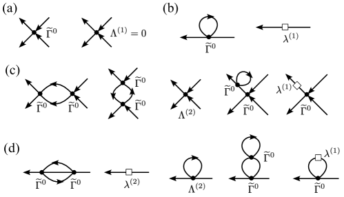
Figure 4: Diagrams to determine the counter term. (a), (b), (c), (d) are diagrams for the first order vertex, first order self-energy, second order vertex, and second order self-energy, respectively.

The second order vertex is contributed by diagrams in Fig. 4(c). The last two diagrams cancel each other because $\widetilde{\Sigma}^{(1)}(\omega)=0$. Then $\Lambda^{(2)}$ should cancel the first two diagrams at zero frequency. We do not attempt to calculate $\Lambda^{(2)}$ in this work.

We also do not attempt to calculate the full second order self-energy $\widetilde{\Sigma}^{(2)}$. Instead, we only show how to calculate its linear frequency-dependence, i.e., $\partial_{\omega}\widetilde{\Sigma}^{(2)}$. The condition $\partial_{\omega}\widetilde{\Sigma}^{(2)}=0$ (Eq. 94) will determine the counter term $\lambda_{0}^{(2)}$. $\widetilde{\Sigma}^{(2)}$ is contributed by the diagrams shown in Fig. 4(d). The last two diagrams cancel each other because $\widetilde{\Sigma}^{(1)}(\omega)=0$ according to the second paragraph above. The third diagram is contributed by $\Lambda^{(2)}$, which by definition is $\omega$-independent (Eq. 91) and hence does not contribute to $\partial_{\omega}\widetilde{\Sigma}^{(2)}$. Thus, we only need to consider the first two diagrams, dubbed as $\Sigma^{(2,1)}$ and $\Sigma^{(2,2)}$, respectively. The first diagram gives the correction

$$\delta\widetilde{\mathcal{G}}^{(2,1)}(1)= -\left\langle f(1)\left(\frac{1}{2}\frac{T^{2}}{4^{2}}\sum_{\begin{subarray}{c}2345\\ 5^{\prime}4^{\prime}3^{\prime}2^{\prime}\end{subarray}}\delta_{\omega_{2}+\omega_{3},\omega_{4}+\omega_{5}}\delta_{\omega_{5}^{\prime}+\omega_{4}^{\prime},\omega_{3}^{\prime}+\omega_{2}^{\prime}}\widetilde{\Gamma}^{0}(23;45)\widetilde{\Gamma}^{0}(5^{\prime}4^{\prime};3^{\prime}2^{\prime})f^{\dagger}(2)f^{\dagger}(3)f(4)f(5)f^{\dagger}(5^{\prime})f^{\dagger}(4^{\prime})f(3^{\prime})f(2^{\prime})\right)f^{\dagger}(1)\right\rangle_{0C}$$ (209)

Applying Wick’s theorem, there is

$$\delta\widetilde{\mathcal{G}}^{(2,1)}(1) =-2^{4}\frac{1}{2}\frac{T^{2}}{4^{2}}\sum_{\begin{subarray}{c}2345\\ 5^{\prime}4^{\prime}3^{\prime}2^{\prime}\end{subarray}}\delta_{\omega_{2}+\omega_{3},\omega_{4}+\omega_{5}}\delta_{\omega_{5}^{\prime}+\omega_{4}^{\prime},\omega_{3}^{\prime}+\omega_{2}^{\prime}}\widetilde{\Gamma}^{0}(23;45)\widetilde{\Gamma}^{0}(5^{\prime}4^{\prime};3^{\prime}2^{\prime})$$

$$\times\wick{\c{1}f(1)\c{1}f^{\dagger}(2)\c{3}f^{\dagger}(3)\c{2}f(4)\c{1}f(5)\c{1}f^{\dagger}(5^{\prime})\c{2}f^{\dagger}(4^{\prime})\c{3}f(3^{\prime})\c{1}f(2^{\prime})\c{1}f^{\dagger}(1)}\ .$$ (210)

The factor $2^{4}$ comes from equivalent contractions. It equals

$$\delta\widetilde{\mathcal{G}}^{(2,1)}(1) =-[\mathcal{G}^{0}(1)]^{2}\cdot\frac{1}{2}\cdot T^{2}\sum_{345}\delta_{\omega_{1}+\omega_{3},\omega_{4}+\omega_{5}}\widetilde{\Gamma}^{0}(13;45)\widetilde{\Gamma}^{0}(54;31)\widetilde{\mathcal{G}}^{0}(3)\widetilde{\mathcal{G}}^{0}(4)\widetilde{\mathcal{G}}^{0}(5)$$ (211)

The self-energy can be extracted as

$$\widetilde{\Sigma}^{(2,1)}(\omega_{1})=-\frac{1}{2}T^{2}\sum_{I_{3,4,5}}|\widetilde{\Gamma}^{0}_{I_{1}I_{3};I_{4}I_{5}}|^{2}\sum_{\omega_{3,4}}\widetilde{\mathcal{G}}^{0}(\omega_{3})\widetilde{\mathcal{G}}^{0}(\omega_{4})\widetilde{\mathcal{G}}^{0}(\omega_{1}+\omega_{3}-\omega_{4})\ ,$$ (212)

where the interaction factor can be calculated as

$$u^{2}=\frac{1}{2}\sum_{I_{3,4,5}}|\widetilde{\Gamma}^{0}_{I_{1}I_{2};I_{3}I_{4}}|^{2}=\frac{1}{16}\sum_{I_{1,2,3,4}}|\widetilde{\Gamma}^{0}_{I_{1}I_{3};I_{4}I_{5}}|^{2}=\frac{1}{16}\mathrm{tr}[\widetilde{\Gamma}^{0}\cdot\widetilde{\Gamma}^{0\dagger}]$$ (213)

Here we regard $I_{1,2}$ and $I_{3,4}$ as the left and right matrix indices respectively. $\mathrm{tr}[\widetilde{\Gamma}^{0}\cdot\widetilde{\Gamma}^{0\dagger}]$ equals the sum of squares of the eigenvalues. $\widetilde{\Gamma}^{0}$ is a 64-dimensional matrix. Its eigenspace with nonzero eigenvalues consists of the 56 anti-symmetric states. Each of the 28 states discussed in Sec. A.5 appears twice in the eigenspace because states related by permutation have been regarded physically identical. Suppose $\Phi_{1}$ is a two-electron state with the energy $E$. Define $\Phi_{2}$ as the permutation of $\Phi_{1}$, it represents the same state. The physical energy is given by the generalized eigenvalue problem defined by the Hamiltonian matrix $H_{nm}=\langle\Phi_{n}|\hat{H}|\Phi_{m}\rangle$ and overlap matrix $S_{nm}=\langle\Phi_{n}|\Phi_{m}\rangle$. There must be $H=E(\sigma_{0}-\sigma_{x})$ and $S=\sigma_{0}-\sigma_{x}$ such that the generalized eigenvalue is $E$. However, the Hamiltonian matrix $H$ itself has two eigenvalues: $2E$ and 0. Therefore, each of 28 two-electron state contribute to an eigenvalue $2E$ and an eigenvalue 0. Thereby,

$$u^{2} = \frac{1}{16}\sum_{E}|2E|^{2}=\frac{1}{4}\left(8\widetilde{U}_{2}^{2}+8\widetilde{U}_{3}^{2}+4\widetilde{U}_{4}^{2}+2(\widetilde{U}_{1}-\widetilde{\mathcal{J}})^{2}+6(\widetilde{U}_{1}+\mathcal{J})^{2}\right)$$ (214)

$$= 2\widetilde{U}_{1}^{2}+2\widetilde{U}_{2}^{2}+2\widetilde{U}_{3}^{2}+\widetilde{U}_{4}^{2}+2\widetilde{U}_{1}\widetilde{\mathcal{J}}+2\widetilde{\mathcal{J}}^{2}\ .$$

Now we have

$$\widetilde{\Sigma}^{(2,1)}(\omega_{1})= -u^{2}\int\frac{d\omega_{3}d\omega_{4}}{(2\pi)^{2}}\cdot\frac{1}{i\omega_{3}+i\widetilde{\Delta}_{0}\mathrm{sgn}(\omega_{3})-\widetilde{\epsilon}_{f}}\frac{1}{i\omega_{4}+i\widetilde{\Delta}_{0}\mathrm{sgn}(\omega_{4})-\widetilde{\epsilon}_{f}}\frac{1}{i(\omega_{1}+\omega_{3}-\omega_{4})+i\widetilde{\Delta}_{0}\mathrm{sgn}(\omega_{1}+\omega_{3}-\omega_{4})-\widetilde{\epsilon}_{f}}$$

$$= -u^{2}\int\frac{d\nu}{2\pi}\cdot F(\nu)\cdot\frac{1}{i(\omega_{1}+\nu)+i\widetilde{\Delta}_{0}\mathrm{sgn}(\omega_{1}+\nu)-\widetilde{\epsilon}_{f}}$$ (215)

where $\nu=\omega_{3}-\omega_{4}$ and

$$F(\nu)=\int\frac{d\omega}{2\pi}\cdot\frac{1}{i\omega+i\widetilde{\Delta}_{0}\mathrm{sgn}(\omega)-\widetilde{\epsilon}_{f}}\cdot\frac{1}{i(\omega-\nu)+i\widetilde{\Delta}_{0}\mathrm{sgn}(\omega-\nu)-\widetilde{\epsilon}_{f}}\ .$$ (216)

By definition $F(\nu)=F(-\nu)$. We hence have

$$F(\nu)= \int_{-\infty}^{0}\frac{d\omega}{2\pi}\frac{1}{i\omega-i\widetilde{\Delta}_{0}-\widetilde{\epsilon}_{f}}\frac{1}{i(\omega-|\nu|)-i\widetilde{\Delta}_{0}-\widetilde{\epsilon}_{f}}+\int_{0}^{|\nu|}\frac{d\omega}{2\pi}\frac{1}{i\omega+i\widetilde{\Delta}_{0}-\widetilde{\epsilon}_{f}}\frac{1}{i(\omega-|\nu|)-i\widetilde{\Delta}_{0}-\widetilde{\epsilon}_{f}}$$

$$+ \int_{|\nu|}^{\infty}\frac{d\omega}{2\pi}\frac{1}{i\omega+i\widetilde{\Delta}_{0}-\widetilde{\epsilon}_{f}}\frac{1}{i(\omega-|\nu|)+i\widetilde{\Delta}_{0}-\widetilde{\epsilon}_{f}}\ ,$$ (217)

Define $z=i\omega$, the above integral along imaginary axes of $z$ can be continuously deformed to integral along real axes:

$$F(\nu)= \int_{0}^{\infty}\frac{dz}{2\pi i}\left(\frac{1}{z+i\widetilde{\Delta}_{0}-\widetilde{\epsilon}_{f}}-c.c.\right)\frac{1}{z-i|\nu|-i\widetilde{\Delta}_{0}-\widetilde{\epsilon}_{f}}+\int_{0}^{\infty}\frac{dz}{2\pi i}\frac{1}{z+i|\nu|+i\widetilde{\Delta}_{0}-\widetilde{\epsilon}_{f}}\left(\frac{1}{z+i\widetilde{\Delta}_{0}-\widetilde{\epsilon}_{f}}-c.c.\right)$$

$$= \frac{2}{\pi}\int_{0}^{\infty}dz\cdot\frac{\widetilde{\Delta}_{0}}{(z-\widetilde{\epsilon}_{f})^{2}+\widetilde{\Delta}_{0}^{2}}\cdot\frac{z-\widetilde{\epsilon}_{f}}{(z-\widetilde{\epsilon}_{f})^{2}+(|\nu|+\widetilde{\Delta}_{0})^{2}}=\frac{\widetilde{\Delta}_{0}}{\pi(\nu^{2}+2\widetilde{\Delta}_{0}|\nu|)}\ln\left(1+\frac{\nu^{2}+2\widetilde{\Delta}_{0}|\nu|}{\widetilde{\Delta}_{0}^{2}+\widetilde{\epsilon}_{f}^{2}}\right)$$ (218)

It is direct to verify that $F(0^{+})=F(0^{-})=\frac{\widetilde{\Delta}_{0}}{\pi(\widetilde{\Delta}_{0}^{2}+\widetilde{\epsilon}_{f}^{2})}=\frac{\sin^{2}\delta_{f}}{\pi\widetilde{\Delta}_{0}}$ is the density of states at the Fermi level. Due to Eq. 140, the leading order $\omega_{1}$-dependence of $\widetilde{\Sigma}^{(2,1)}$ can be obtained as

$$\partial_{\omega}\widetilde{\Sigma}^{(2,1)}(\omega)= -i\cdot u^{2}\int\frac{d\nu}{2\pi}\cdot F(\nu)\left([\widetilde{\mathcal{G}}^{0}(\nu)]^{2}+2\pi\cdot\frac{\sin^{2}\delta_{f}}{\pi\widetilde{\Delta}_{0}}\delta(\nu)\right)$$

$$= -i\cdot\left(\frac{u\cdot\sin^{2}\delta_{f}}{\pi\widetilde{\Delta}_{0}}\right)^{2}-i\cdot u^{2}\int_{0}^{\infty}\frac{d\nu}{2\pi}\cdot F(\nu)\frac{2\widetilde{\epsilon}_{f}^{2}-2(\nu+\widetilde{\Delta}_{0})^{2}}{(\widetilde{\epsilon}_{f}^{2}+(\nu+\widetilde{\Delta}_{0})^{2})^{2}}$$ (219)

We define the dimensionless function

$$\xi^{2}(\delta_{f})=\sin^{4}\delta_{f}+\pi^{2}\int_{0}^{\infty}\frac{dx}{2\pi}\cdot\frac{1}{\pi(x^{2}+2x)}\ln\left(1+\frac{x^{2}+2x}{1+\cot^{2}\delta_{f}}\right)\frac{2\cot^{2}(\delta_{f})-2(1+x)^{2}}{[\cot^{2}(\delta_{f})+(1+x)^{2}]^{2}}$$ (220)

then we can write $\partial_{\omega}\widetilde{\Sigma}^{(2,1)}(\omega)$ as

$$\partial_{\omega}\widetilde{\Sigma}^{(2,1)}(\omega)=-i\left(\frac{u\cdot\xi(\delta_{f})}{\pi\widetilde{\Delta}_{0}}\right)^{2}$$ (221)

We find

$$\xi\left(\frac{\pi}{2}\right)=\sqrt{3-\frac{\pi^{2}}{4}}\approx 0.7298,\qquad\xi\left(\frac{\pi}{4}\right)=\sqrt{\frac{4-4\mathcal{C}+\pi-\pi\ln 2}{8}}\approx 0.4031\ ,$$ (222)

where $\mathcal{C}\approx 0.915966$ is the Catalan’s constant. The result $\xi(\pi/2)$ can also be found in Ref. Hewson (1993a). The total frequency derivative $\widetilde{\Sigma}^{(2)}$ also contains the contribution from the second diagram of Fig. 4(d), i.e., $-i\lambda_{0}^{(2)}$. Imposing $\partial_{\omega}\widetilde{\Sigma}^{(2)}=0$ gives

$$\lambda^{(2)}_{0}=-\left(\frac{u\cdot\xi(\delta_{f})}{\pi\widetilde{\Delta}_{0}}\right)^{2}\ .$$ (223)

Appendix C Quasi-particle mean-field theory of the superconductivity

C.1 Effective BdG Hamiltonian

The free part of topological heavy fermion model is given by Song and Bernevig (2022)

$${H}_{0}=-\mu\sum_{\mathbf{R}\alpha\eta s}f_{\mathbf{R}\alpha\eta s}^{\dagger}f_{\mathbf{R}\alpha\eta s}+\sum_{\eta s}\sum_{aa^{\prime}}\sum_{|\mathbf{k}|<\Lambda_{c}}(H^{(c,\eta)}_{aa^{\prime}}(\mathbf{k})-\mu\delta_{aa^{\prime}})c^{\dagger}_{\mathbf{k}a\eta s}c_{\mathbf{k}a\eta s}+\sum_{\eta s\alpha a}\sum_{|\mathbf{k}|<\Lambda_{c}}\left(e^{-\frac{|\mathbf{k}|^{2}\lambda^{2}}{2}}H^{(cf,\eta)}_{a\alpha}(\mathbf{k})c^{\dagger}_{\mathbf{k}a\eta s}f_{\mathbf{k}\alpha\eta s}+h.c.\right)$$ (224)

Here $\mu$ is the chemical potential, $c_{\mathbf{k}a\eta s}$ is the fermion operator for the $c$-electron of the momentum $\mathbf{k}$, orbital $a$ ($=1,2,3,4$), valley $\eta$ ($=\pm$), and spin $s$ ($=\uparrow,\downarrow$), $f_{\mathbf{R}\alpha\eta s}$ is the fermion operator for the $f$-electron of the site $\mathbf{R}$ orbital $\alpha$ (=1,2), valley $\eta$, and spin. $\mathbf{R}$’s form the triangular lattice generated by the Bravais lattice basis $\mathbf{a}_{\rm M1}=\frac{2\pi}{3k_{\theta}}(\sqrt{3},1)$, $\mathbf{a}_{\rm M2}=\frac{2\pi}{3k_{\theta}}(-\sqrt{3},1)$, where $k_{\theta}=2|\mathbf{K}|\sin\frac{\theta}{2}$, $\theta=1.08^{\circ}$ is the first magic angle, $|\mathbf{K}|=1.703\mathring{A}^{-1}$. The triangular lattice corresponds to the AA stacking regions of MATBG (Fig. 1(a)). $f_{\mathbf{k}\alpha\eta s}=\frac{1}{N_{M}}\sum_{\mathbf{R}}e^{-i\mathbf{R}\cdot\mathbf{k}}f_{\mathbf{R}\alpha\eta s}$ is the $f$-electron operator at the momentum $\mathbf{k}$, with $N_{\rm M}$ being the number of moiré cells and $\mathbf{k}$ taking values in the moiré Brillouin zone spanned by $\mathbf{b}_{\rm M1}=k_{\theta}(\frac{\sqrt{2}}{2},\frac{3}{2})$, $\mathbf{b}_{\rm M2}=k_{\theta}(-\frac{\sqrt{2}}{2},\frac{3}{2})$. However, $c$-electron is described by a continuous field that cannot be regularized to a lattice due to the symmetry anomaly Song et al. (2021). Thus, momentum $\mathbf{k}$ of $c$-electrons is within a cutoff $\Lambda_{c}$ that will be sent to infinity in the end Song and Bernevig (2022). The matrices $H^{(c,\eta)}$ and $H^{(cf,\eta)}$ are defined by

$$H^{(c,\eta)}(\mathbf{k})=\begin{pmatrix}0_{2\times 2}&v_{\star}(\eta k_{x}\sigma^{0}+ik_{y}\sigma^{z})\\ v_{\star}(\eta k_{x}\sigma^{0}-ik_{y}\sigma^{z})&M\sigma^{x}\end{pmatrix},\qquad H^{(cf,\eta)}(\mathbf{k})=\begin{pmatrix}\gamma\sigma^{0}+v_{\star}^{\prime}(\eta k_{x}\sigma^{x}+k_{y}\sigma^{y})\\ 0_{2\times 2}\end{pmatrix}\ .$$ (225)

The parameter $\lambda$ is the spread of the Wannier functions of $f$-electrons, and it suppresses the hybridization at large momentum. In this work we adopt the parameters: $\gamma=-24.75$meV, $v_{\star}=-4.303\mathrm{eV\cdot\mathring{A}}$, $v_{\star}^{\prime}=1.623\mathrm{eV\cdot\mathring{A}}$, $\lambda=1.4131/k_{\theta}$, $M=3.697$meV. The resulting band structure is shown in the inset of Fig. 1(a).

The free Hamiltonian has time-reversal $T$ and $D_{6}$ point group, generated by $C_{2z}$-rotation, $C_{3z}$-rotation, and $C_{2x}$-rotation symmetries. Their representations on $f$-electrons and $c$-electrons are given by (Eq. 8)

$$T=\sigma^{0}\tau^{x}\varsigma^{0}K,\qquad C_{2z}=\sigma^{x}\tau^{x}\varsigma^{0},\qquad C_{3z}=e^{i\frac{2\pi}{3}\sigma^{z}\tau^{z}\varsigma^{0}},\qquad C_{2x}=\sigma^{x}\tau^{0}\varsigma^{0}\ ,$$ (226)

and

$$T=(\sigma^{0}\tau^{x}\varsigma^{0}\oplus\sigma^{0}\tau^{x}\varsigma^{0})K,\qquad C_{2z}=\sigma^{x}\tau^{x}\varsigma^{0}\oplus\sigma^{x}\tau^{x}\varsigma^{0},\qquad C_{3z}=e^{i\frac{2\pi}{3}\sigma^{z}\tau^{z}\varsigma^{0}}\oplus\sigma^{0}\tau^{0}\varsigma^{0},\qquad C_{2x}=\sigma^{x}\tau^{0}\varsigma^{0}\oplus\sigma^{x}\tau^{0}\varsigma^{0}\ ,$$ (227)

respectively. Detailed derivations of these symmetries are given sections S2A and S2B of the supplementary material Ref. Song and Bernevig (2022). Readers may directly verify that Eq. 224 is invariant under these symmetries. In this work we do not distinguish the single-particle and the second-quantized representations of symmetry operators. The correspondence between the two representations are given after Eq. 8.

Eq. 224 with Coulomb interaction is solved within the framework of dynamical mean-field theory (DMFT) in Refs. Zhou et al. (2023); Datta et al. (2023); Rai et al. (2023). Here we are only interested in the doped correlated insulator at the filling $\nu=-2-\delta\nu$, where the $\widetilde{\Delta}_{0}\ll\mathcal{J}$ is assumed. In the mean-field calculations, we will regard $z$ as an additional input to $\delta\nu$. In the $\widetilde{\Delta}_{0}\ll\mathcal{J}$ limit, the $f$-filling is frozen to $\nu_{f}=-2$, indicating that the doping is fully undertaken by $c$-electrons, i.e., $\nu_{c}=\nu-\nu_{f}=-\delta\nu$.

To describe the quasi-particles at $\nu=-2-\delta\nu$, we express $f$-electron operators in terms of the quasi-particles operators as $f_{\mathbf{R}\alpha\eta s}=z^{\frac{1}{2}}\widetilde{f}_{\mathbf{R}\alpha\eta s}$. We also introduce the DMFT self-consistent on-site energies $\epsilon_{f}$, $\epsilon_{c1}=\epsilon_{c2}$, $\epsilon_{c3}=\epsilon_{c4}$ for $\widetilde{f}$-electrons, $a=1,2$ $c-$electrons, $a=3,4$ $c$-electrons, respectively Zhou et al. (2023). Then the effective free Hamiltonian for the quasi-particle can be written as

$${H}_{0}= \epsilon_{f}\sum_{\mathbf{R}\alpha\eta s}\widetilde{f}_{\mathbf{R}\alpha\eta s}^{\dagger}\widetilde{f}_{\mathbf{R}\alpha\eta s}+\sum_{\eta s}\sum_{aa^{\prime}}\sum_{|\mathbf{k}|<\Lambda_{c}}(H^{(c,\eta)}_{aa^{\prime}}(\mathbf{k})+\delta_{aa^{\prime}}\epsilon_{c,a})c^{\dagger}_{\mathbf{k}a\eta s}c_{\mathbf{k}a\eta s}$$

$$+z^{\frac{1}{2}}\sum_{\eta s\alpha a}\sum_{|\mathbf{k}|<\Lambda_{c}}\left(e^{-\frac{|\mathbf{k}|^{2}\lambda^{2}}{2}}H^{(cf,\eta)}_{a\alpha}(\mathbf{k})c^{\dagger}_{\mathbf{k}a\eta s}\widetilde{f}_{\mathbf{k}\alpha\eta s}+h.c.\right)\ .$$ (228)

One can see that the $cf$ hybridization is suppressed by $z^{\frac{1}{2}}$. $\epsilon_{f}$, $\epsilon_{c,1}$, $\epsilon_{c,3}$ should be determined self-consistently in the DMFT plus Hartree-Fock calculations. Here we provide a quick approach to estimate $\epsilon_{f}$, $\epsilon_{c,1}$, $\epsilon_{c,3}$ for given $z$ and $\nu=-2-\delta\nu$. First, it is found that $G=\epsilon_{c,3}-\epsilon_{c,1}$ is insensitive to doping and can be approximated as a fixed quantity (taken as 8meV here) Zhou et al. (2023). We then search for $\epsilon_{f}$ and $\epsilon_{c,1}$ that give the correct fillings $\nu_{f}=-2$ and $\nu_{c}=-\delta\nu$.

As detailed in Appendix B.5, we take the irreducible vertex $z^{2}\Gamma^{\rm p}$ - multiplied by $z^{2}$ - in the pairing channel as the effective interaction in mean-field calculation. (One would over-count Feynman diagrams if $z^{2}\Gamma$ is used instead Georges et al. (1996).) For the sake of investigating superconducting orders, it suffices to keep the strongest channel in $\Gamma^{\rm p}$, i.e., the $d$-wave $E_{2}$ states (Eq. 64). At $\nu_{f}=-2$, the pairing potential is determined by the renormalized interaction $\widetilde{\mathcal{J}}$ via (Eq. 195)

$$U^{\rm p}_{1}-\mathcal{J}^{\rm p}\approx\frac{-2\pi\widetilde{\Delta}_{0}-\widetilde{\mathcal{J}}}{1+\frac{\pi}{2}+\widetilde{\mathcal{J}}/(4\widetilde{\Delta}_{0})},\qquad 4.6\widetilde{\Delta}_{0}\lesssim\widetilde{\mathcal{J}}\lesssim 10.3\widetilde{\Delta}_{0}\ .$$ (229)

The explicit form of the corresponding interaction can be constructed as projectors to Eq. 64

$$H_{\rm p}= (U_{1}^{\rm p}-\mathcal{J}^{\rm p})\sum_{\mathbf{R}}\sum_{\eta}\frac{(\widetilde{f}_{\mathbf{R}1\eta\uparrow}^{\dagger}\widetilde{f}_{\mathbf{R}2\overline{\eta}\downarrow}^{\dagger}-\widetilde{f}_{\mathbf{R}1\eta\downarrow}^{\dagger}\widetilde{f}_{\mathbf{R}2\overline{\eta}\uparrow}^{\dagger})(\widetilde{f}_{\mathbf{R}2\overline{\eta}\downarrow}\widetilde{f}_{\mathbf{R}1\eta\uparrow}-\widetilde{f}_{\mathbf{R}2\overline{\eta}\uparrow}\widetilde{f}_{\mathbf{R}1\eta\downarrow})}{2}$$

$$= \frac{U_{1}^{\rm p}-\mathcal{J}^{\rm p}}{2}\sum_{\mathbf{R}}\sum_{\eta}(\widetilde{f}_{\mathbf{R}2\overline{\eta}\downarrow}^{\dagger}\widetilde{f}_{\mathbf{R}1\eta\uparrow}^{\dagger}-\widetilde{f}_{\mathbf{R}2\overline{\eta}\uparrow}^{\dagger}\widetilde{f}_{\mathbf{R}1\eta\downarrow}^{\dagger})(\widetilde{f}_{\mathbf{R}1\eta\uparrow}\widetilde{f}_{\mathbf{R}2\overline{\eta}\downarrow}-\widetilde{f}_{\mathbf{R}1\eta\downarrow}\widetilde{f}_{\mathbf{R}2\overline{\eta}\uparrow})\ .$$ (230)

We only consider the order parameters

$$\Psi_{\eta}=\langle\Phi_{\rm G}|\widetilde{f}_{\mathbf{R}1\eta\uparrow}\widetilde{f}_{\mathbf{R}2\overline{\eta}\downarrow}|\Phi_{\rm G}\rangle\ .$$ (231)

where $\Phi_{\rm G}$ is the ground state. Due to the spin-SU(2) symmetry ($i\varsigma^{y})$, there must be

$$\Psi_{\eta}=-\langle\Phi_{G}|\widetilde{f}_{\mathbf{R}1\eta\downarrow}\widetilde{f}_{\mathbf{R}2\overline{\eta}\uparrow}|\Phi_{G}\rangle\ .$$ (232)

The mean-field decomposition of $H_{\rm p}$ reads

$$H_{\rm p}\approx \frac{U^{\rm p}_{1}-\mathcal{J}^{\rm p}}{2}\sum_{\mathbf{R}\eta}\Big{[}2\Psi_{\eta}(\widetilde{f}^{\dagger}_{\mathbf{R}2\overline{\eta}\downarrow}\widetilde{f}^{\dagger}_{\mathbf{R}1\eta\uparrow}-\widetilde{f}^{\dagger}_{\mathbf{R}2\overline{\eta}\uparrow}\widetilde{f}^{\dagger}_{\mathbf{R}1\eta\downarrow})+2\Psi_{\eta}^{*}(\widetilde{f}_{\mathbf{R}1\eta\uparrow}\widetilde{f}_{\mathbf{R}2\overline{\eta}\downarrow}-\widetilde{f}_{\mathbf{R}1\eta\downarrow}\widetilde{f}_{\mathbf{R}2\overline{\eta}\uparrow})-2|\Psi_{\eta}|^{2}\Big{]}$$ (233)

We can see that $(\eta,s)=(+,\uparrow)$ electrons only couples to $(-,\downarrow)$ electrons, whereas $(-,\uparrow)$ electrons only couples to $(+,\downarrow)$ electrons. Thus, the BdG Hamiltonian is block diagonal. We can write the total Hamiltonian as

$$H\approx -N_{\rm M}(U^{\rm p}_{1}-\mathcal{J}^{\rm p})(|\Psi_{+}|^{2}+|\Psi_{-}|^{2})+\overline{H}_{+}+\overline{H}_{-}$$ (234)

$\overline{H}_{+}$ is the BdG Hamiltonian for the $(\eta,s)=(+,\uparrow)$ and $(-,\downarrow)$ electrons

$$\overline{H}_{+}= \sum_{\mathbf{k}}\begin{pmatrix}\widetilde{f}_{\mathbf{k}+\uparrow}^{\dagger}&c_{\mathbf{k}+\uparrow}^{\dagger}&\widetilde{f}_{-\mathbf{k}-\downarrow}&c_{-\mathbf{k}-\downarrow}\end{pmatrix}\begin{pmatrix}\widetilde{\epsilon}_{f}&z^{\frac{1}{2}}\mathcal{H}^{(cf,+)\dagger}(\mathbf{k})&\mathcal{V}&0\\ z^{\frac{1}{2}}\mathcal{H}^{(cf,+)}(\mathbf{k})&\mathcal{H}^{(c,+)}(\mathbf{k})&0&0\\ \mathcal{V}^{\dagger}&0&-\widetilde{\epsilon}_{f}&-z^{\frac{1}{2}}\mathcal{H}^{(cf,-)T}(-\mathbf{k})\\ 0&0&-z^{\frac{1}{2}}\mathcal{H}^{(cf,-)*}(-\mathbf{k})&-\mathcal{H}^{(c,-)T}(-\mathbf{k})\end{pmatrix}\begin{pmatrix}\widetilde{f}_{\mathbf{k}+\uparrow}\\ c_{\mathbf{k}+\uparrow}\\ \widetilde{f}_{-\mathbf{k}-\downarrow}^{\dagger}\\ c_{-\mathbf{k}-\downarrow}^{\dagger}\end{pmatrix}$$ (235)

where

$$\mathcal{V}=-(U^{\rm p}_{1}-\mathcal{J}^{\rm p})\begin{pmatrix}0&\Psi_{+}\\ \Psi_{-}&0\end{pmatrix}\ ,$$ (236)

is a two-by-two matrix. Here $\widetilde{f}_{\mathbf{k}+\uparrow}$ and $\widetilde{f}_{-\mathbf{k}-\downarrow}^{\dagger}$ are column vectors consisting of $\widetilde{f}_{\mathbf{k}\alpha+\uparrow}$ and $\widetilde{f}_{-\mathbf{k}\alpha-\downarrow}^{\dagger}$, respectively. $c_{\mathbf{k}+\uparrow}$ and $c_{-\mathbf{k}-\downarrow}$ are column vectors consisting of $c_{\mathbf{k}+\mathbf{G},a+\uparrow}$ and $c_{-\mathbf{k}-\mathbf{G},a-\downarrow}$, respectively, where $\mathbf{k}$ is in the moiré Brillouin zone and $\mathbf{G}$, regarded as a matrix index, is moiré reciprocal lattice. The $\mathcal{H}^{(c,\eta)}$ and $\mathcal{H}^{(cf,\eta)}$ matrices are defined as

$$\mathcal{H}^{(c,\eta)}_{\mathbf{G}a,\mathbf{G}^{\prime}a^{\prime}}(\mathbf{k})=\delta_{\bf G,G^{\prime}}\left(\epsilon_{c,a}\delta_{aa^{\prime}}+H^{(c,\eta)}_{aa^{\prime}}(\mathbf{k}+\mathbf{G})\right),\qquad\mathcal{H}^{(cf,\eta)}_{\mathbf{G}a,\alpha}(\mathbf{k})=e^{-\frac{|\mathbf{k}+\mathbf{G}|^{2}\lambda^{2}}{2}}H^{(cf,\eta)}_{a\alpha}(\mathbf{k}+\mathbf{G})\ .$$ (237)

$\overline{H}_{-}$ is the BdG Hamiltonian for $(\eta,s)=(+,\downarrow),(-,\uparrow)$ electrons. It can be obtained by applying the $i\varsigma^{y}$ rotation to $\overline{H}_{+}$, and hence it has identical spectrum as $\overline{H}_{+}$. The total energy (per moiré unit cell) can be calculated as

$$\frac{E_{\rm tot}}{N_{\rm M}}=-N_{\rm M}(U^{\rm p}_{1}-\mathcal{J}^{\rm p})(|\Psi_{+}|^{2}+|\Psi_{-}|^{2})+\frac{2}{N_{\rm M}}\sum_{n\in{\rm occ}}\sum_{\mathbf{k}}\mathcal{E}_{n\mathbf{k}}\ ,$$ (238)

where $\mathcal{E}_{n\mathbf{k}}$ is the $n$-th BdG band of $\overline{H}_{+}$, and “$\sum_{n\in{\rm occ}}$” means summation over the negative branches.

There are two relevant saddle points of the pairings in the numerical calculation:

$$\mathcal{V}=e^{i\theta_{1}}\mathcal{V}_{1}(\cos\varphi\cdot\sigma^{x}+\sin\varphi\cdot\sigma^{y}),\quad e^{i\theta_{2}}\mathcal{V}_{2}\frac{\sigma^{x}\pm i\sigma^{y}}{2}\ .$$ (239)

Here $\mathcal{V}_{1}$ ($>0$), $\mathcal{V}_{2}$ ($>0$) represent the pairing mean-field Hamiltonian terms

$$e^{i\theta_{1}}\mathcal{V}_{1}\sum_{\mathbf{k}}\left[e^{-i\varphi}\widetilde{f}_{\mathbf{k}1+\uparrow}^{\dagger}\widetilde{f}_{-\mathbf{k}2-\downarrow}^{\dagger}+e^{i\varphi}\widetilde{f}_{\mathbf{k}2+\uparrow}^{\dagger}\widetilde{f}_{-\mathbf{k}1-\downarrow}^{\dagger}\right]-(\uparrow\leftrightarrow\downarrow)\ .$$ (240)

$$e^{i\theta_{2}}\mathcal{V}_{2}\sum_{\mathbf{k}}\widetilde{f}_{\mathbf{k}1+\uparrow}^{\dagger}\widetilde{f}_{-\mathbf{k}2-\downarrow}^{\dagger}-(\uparrow\leftrightarrow\downarrow)\quad\text{or}\quad e^{i\theta_{2}}\mathcal{V}_{2}\sum_{\mathbf{k}}\widetilde{f}_{\mathbf{k}2+\uparrow}^{\dagger}\widetilde{f}_{-\mathbf{k}1-\downarrow}^{\dagger}-(\uparrow\leftrightarrow\downarrow)\ ,$$ (241)

respectively. $\theta_{1,2}$ are the U(1) phases spontaneously chosen in the symmetry breaking. $\sum_{\mathbf{k}}\widetilde{f}_{\mathbf{k}1+\uparrow}^{\dagger}\widetilde{f}_{-\mathbf{k}2-\downarrow}^{\dagger}-\widetilde{f}_{\mathbf{k}1+\downarrow}^{\dagger}\widetilde{f}_{-\mathbf{k}2-\uparrow}^{\dagger}$ and $\sum_{\mathbf{k}}\widetilde{f}_{\mathbf{k}2+\uparrow}^{\dagger}\widetilde{f}_{-\mathbf{k}1-\downarrow}^{\dagger}-\widetilde{f}_{\mathbf{k}2+\downarrow}^{\dagger}\widetilde{f}_{-\mathbf{k}1-\uparrow}^{\dagger}$ transform as $d_{x^{2}-y^{2}}\pm id_{xy}$ orbitals under the symmetry operations and form the two-dimensional representation $E_{2}$ of $D_{6}$ (Eq. 226). The linear combination in Eq. 240 breaks the $C_{3z}$ symmetry and respects $C_{2z}$ and time-reversal ($T=\tau^{x}K$) symmetries. The linear combinations in Eq. 241 break the time-reversal symmetry and preserve $C_{6z}$. Thus, $\mathcal{V}_{1}$ and $\mathcal{V}_{2}$ correspond to the nematic $d$-wave pairing and chiral $d$-wave pairing, respectively. As we will show in next subsubsection, $\mathcal{V}_{1}$ leads to a $p$-wave-like nodal structure in the BdG spectrum due to the Berry’s phase on Fermi surface.

C.2 The $p$-wave-like nodal structure in the nematic $d$-wave phase

We now show that the $\mathcal{V}_{1}$ pairing leads to a $p$-wave-like nodal structure in the BdG spectrum. We consider the weak pairing limit and project Eq. 235 onto the Fermi surface basis. As shown in Fig. 3(b), there are two Fermi surfaces around the $\Gamma_{M}$ point, and both of them are dominated by the $f$-orbitals. For either Fermi surface, we can approximate the Bloch band state around the Fermi surface as

$$\psi_{\mathbf{k}\eta s}^{\dagger}=\sum_{\alpha}U^{(\eta)}_{\alpha}(\mathbf{k})\widetilde{f}^{\dagger}_{\mathbf{k}\alpha\eta s}\ .$$ (242)

The time-reversal $T=\tau^{x}K$ and $C_{2z}T=\sigma^{x}K$ symmetries (Eq. 226) indicate

$$T\psi_{\mathbf{k}+s}^{\dagger}T^{-1}=\psi_{-\mathbf{k}-s}^{\dagger}\quad\Rightarrow\quad U_{\alpha}^{(-)}(-\mathbf{k})=U_{\alpha}^{(+)*}(\mathbf{k})$$ (243)

$$C_{2z}T\psi_{\mathbf{k}+s}^{\dagger}(C_{2z}T)^{-1}=\psi_{\mathbf{k}+s}^{\dagger}e^{i\phi_{\mathbf{k}}}\quad\Rightarrow\quad U_{2}^{(+)}(\mathbf{k})=U_{1}^{(+)*}(\mathbf{k})e^{-i\phi_{\mathbf{k}}}\ .$$ (244)

Without loss of generality, we can choose the gauge

$$U^{(+)}(\mathbf{k})=\frac{1}{\sqrt{2}}\begin{pmatrix}1\\ e^{-i\phi_{\mathbf{k}}}\end{pmatrix},\qquad U^{(-)}(-\mathbf{k})=\frac{1}{\sqrt{2}}\begin{pmatrix}1\\ e^{i\phi_{\mathbf{k}}}\end{pmatrix}\ .$$ (245)

According to Ref. Ahn et al. (2019), $\phi_{\mathbf{k}}$ must have an odd winding number along the Fermi surface, i.e.,

$$\mathcal{W}=\frac{1}{2\pi}\oint_{\rm FS}d\mathbf{k}\cdot\partial_{\mathbf{k}}\phi_{\mathbf{k}}=1\mod 2\ ,$$ (246)

if the Fermi surface encloses an odd number of Dirac points. In the symmetric Fermi liquid, $\phi_{\mathbf{k}}$ winding number is $\pm 1$, as shown in Fig. 3(b). Now we project the $\mathcal{V}_{1}$ pairing onto the Fermi surface

$$\sum_{\mathbf{k}}e^{i\theta_{1}}\mathcal{V}_{1}\left(e^{-i\varphi}\widetilde{f}_{\mathbf{k}1+\uparrow}^{\dagger}\widetilde{f}_{-\mathbf{k}2-\downarrow}^{\dagger}+e^{i\varphi}\widetilde{f}_{\mathbf{k}2+\uparrow}^{\dagger}\widetilde{f}_{-\mathbf{k}1-\downarrow}^{\dagger}\right)-(\uparrow\leftrightarrow\downarrow)$$

$$= \sum_{\mathbf{k}}2e^{i\theta_{1}}\mathcal{V}_{1}\cdot\cos(\phi_{\mathbf{k}}+\varphi)\cdot\psi_{\mathbf{k}+\uparrow}^{\dagger}\psi_{-\mathbf{k}-\downarrow}^{\dagger}-(\uparrow\leftrightarrow\downarrow)\ .$$ (247)

As $\phi_{\mathbf{k}}$ winds $\pm 2\pi$ along the Fermi surface, there will be two nodes.

The nodes are robust against perturbations that preserve the $C_{2z}T$ symmetry. For example, we consider a mixture of $s$-wave pairing and the nematic $d$-wave pairing. Due to the $D_{6}$ point group symmetry, the $s$-wave pairing must have the form $e^{i\theta_{0}}\cdot\mathcal{V}_{0}\sigma^{0}$ ($\mathcal{V}_{0}>0$). The projected pairing on Fermi surface becomes

$$\sum_{\mathbf{k}}e^{i\theta_{0}}\mathcal{V}_{0}\left(\widetilde{f}_{\mathbf{k}1+\uparrow}^{\dagger}\widetilde{f}_{-\mathbf{k}1-\downarrow}^{\dagger}+\widetilde{f}_{\mathbf{k}2+\uparrow}^{\dagger}\widetilde{f}_{-\mathbf{k}2-\downarrow}^{\dagger}\right)+e^{i\theta_{1}}\mathcal{V}_{1}\left(e^{-i\varphi}\widetilde{f}_{\mathbf{k}1+\uparrow}^{\dagger}\widetilde{f}_{-\mathbf{k}2-\downarrow}^{\dagger}+e^{i\varphi}\widetilde{f}_{\mathbf{k}2+\uparrow}^{\dagger}\widetilde{f}_{-\mathbf{k}1-\downarrow}^{\dagger}\right)-(\uparrow\leftrightarrow\downarrow)$$

$$= \sum_{\mathbf{k}}2\left(e^{i\theta_{0}}\mathcal{V}_{0}+e^{i\theta_{1}}\mathcal{V}_{1}\cdot\cos(\phi_{\mathbf{k}}+\varphi)\right)\psi_{\mathbf{k}+\uparrow}^{\dagger}\psi_{-\mathbf{k}-\downarrow}^{\dagger}-(\uparrow\leftrightarrow\downarrow)\ .$$ (248)

The $C_{2z}T$ symmetry requires $\theta_{0}=\theta_{1}$ mod $\pi$ such that the pairing term gains a uniform phase $e^{-i2\theta_{0}}$ under $C_{2z}T$. There are two pairing nodes on the Fermi surface as long as $\mathcal{V}_{0}<\mathcal{V}_{1}$.

The above discussions are based on the weak pairing presumption. If the pairing energy is much larger than the band separation, then the nodes on inner and outer Fermi surfaces will merge each other, leading to a gapped phase.

Refs. Wu et al. (2018); Liu et al. (2023) reported that the $d$-wave pairing has four nodes on the Fermi surface. The difference is because Refs. Wu et al. (2018); Liu et al. (2023) used the bare band structure of MATBG, where $\phi_{\mathbf{k}}$ has a winding number 2.

References

• Bistritzer and MacDonald (2011) Rafi Bistritzer and Allan H. MacDonald, “Moiré bands in twisted double-layer graphene,” Proceedings of the National Academy of Sciences 108, 12233–12237 (2011).
• Cao et al. (2018a) Yuan Cao, Valla Fatemi, Shiang Fang, Kenji Watanabe, Takashi Taniguchi, Efthimios Kaxiras,  and Pablo Jarillo-Herrero, “Unconventional superconductivity in magic-angle graphene superlattices,” Nature 556, 43–50 (2018a).
• Cao et al. (2018b) Yuan Cao, Valla Fatemi, Ahmet Demir, Shiang Fang, Spencer L. Tomarken, Jason Y. Luo, Javier D. Sanchez-Yamagishi, Kenji Watanabe, Takashi Taniguchi, Efthimios Kaxiras, Ray C. Ashoori,  and Pablo Jarillo-Herrero, “Correlated insulator behaviour at half-filling in magic-angle graphene superlattices,” Nature 556, 80–84 (2018b).
• Lu et al. (2019) Xiaobo Lu, Petr Stepanov, Wei Yang, Ming Xie, Mohammed Ali Aamir, Ipsita Das, Carles Urgell, Kenji Watanabe, Takashi Taniguchi, Guangyu Zhang, Adrian Bachtold, Allan H. MacDonald,  and Dmitri K. Efetov, “Superconductors, orbital magnets and correlated states in magic-angle bilayer graphene,” Nature 574, 653–657 (2019).
• Yankowitz et al. (2019) Matthew Yankowitz, Shaowen Chen, Hryhoriy Polshyn, Yuxuan Zhang, K. Watanabe, T. Taniguchi, David Graf, Andrea F. Young,  and Cory R. Dean, “Tuning superconductivity in twisted bilayer graphene,” Science 363, 1059–1064 (2019).
• Oh et al. (2021) Myungchul Oh, Kevin P. Nuckolls, Dillon Wong, Ryan L. Lee, Xiaomeng Liu, Kenji Watanabe, Takashi Taniguchi,  and Ali Yazdani, “Evidence for unconventional superconductivity in twisted bilayer graphene,” Nature 600, 240–245 (2021).
• Cao et al. (2021) Yuan Cao, Daniel Rodan-Legrain, Jeong Min Park, Noah F. Q. Yuan, Kenji Watanabe, Takashi Taniguchi, Rafael M. Fernandes, Liang Fu,  and Pablo Jarillo-Herrero, “Nematicity and competing orders in superconducting magic-angle graphene,” Science 372, 264–271 (2021), publisher: American Association for the Advancement of Science.
• Cao et al. (2020) Yuan Cao, Debanjan Chowdhury, Daniel Rodan-Legrain, Oriol Rubies-Bigorda, Kenji Watanabe, Takashi Taniguchi, T. Senthil,  and Pablo Jarillo-Herrero, “Strange Metal in Magic-Angle Graphene with near Planckian Dissipation,” Physical Review Letters 124, 076801 (2020), publisher: American Physical Society.
• Polshyn et al. (2019) Hryhoriy Polshyn, Matthew Yankowitz, Shaowen Chen, Yuxuan Zhang, K. Watanabe, T. Taniguchi, Cory R. Dean,  and Andrea F. Young, “Large linear-in-temperature resistivity in twisted bilayer graphene,” Nature Physics , 1–6 (2019).
• Jaoui et al. (2022) Alexandre Jaoui, Ipsita Das, Giorgio Di Battista, Jaime Díez-Mérida, Xiaobo Lu, Kenji Watanabe, Takashi Taniguchi, Hiroaki Ishizuka, Leonid Levitov,  and Dmitri K. Efetov, “Quantum critical behaviour in magic-angle twisted bilayer graphene,” Nature Physics 18, 633–638 (2022).
• Wu et al. (2018) Fengcheng Wu, A. H. MacDonald,  and Ivar Martin, “Theory of Phonon-Mediated Superconductivity in Twisted Bilayer Graphene,” Physical Review Letters 121, 257001 (2018), publisher: American Physical Society.
• Lian et al. (2019) Biao Lian, Zhijun Wang,  and B. Andrei Bernevig, “Twisted Bilayer Graphene: A Phonon-Driven Superconductor,” Physical Review Letters 122, 257002 (2019).
• Liu et al. (2023) Chao-Xing Liu, Yulin Chen, Ali Yazdani,  and B. Andrei Bernevig, “Electron-K-Phonon Interaction In Twisted Bilayer Graphene,”  (2023), arXiv:2303.15551 [cond-mat].
• Yu et al. (2022) Jiabin Yu, Ming Xie, Fengcheng Wu,  and Sankar Das Sarma, “Euler Obstructed Cooper Pairing in Twisted Bilayer Graphene: Nematic Nodal Superconductivity and Bounded Superfluid Weight,”  (2022), arXiv:2202.02353 [cond-mat].
• You and Vishwanath (2019) Yi-Zhuang You and Ashvin Vishwanath, “Superconductivity from valley fluctuations and approximate SO(4) symmetry in a weak coupling theory of twisted bilayer graphene,” npj Quantum Materials 4, 1–12 (2019).
• Khalaf et al. (2021) Eslam Khalaf, Shubhayu Chatterjee, Nick Bultinck, Michael P. Zaletel,  and Ashvin Vishwanath, “Charged skyrmions and topological origin of superconductivity in magic-angle graphene,” Science Advances 7, eabf5299 (2021), publisher: American Association for the Advancement of Science.
• Christos et al. (2023) Maine Christos, Subir Sachdev,  and Mathias S. Scheurer, “Nodal band-off-diagonal superconductivity in twisted graphene superlattices,” Nature Communications 14, 7134 (2023), number: 1 Publisher: Nature Publishing Group.
• Stepanov et al. (2020) Petr Stepanov, Ipsita Das, Xiaobo Lu, Ali Fahimniya, Kenji Watanabe, Takashi Taniguchi, Frank H. L. Koppens, Johannes Lischner, Leonid Levitov,  and Dmitri K. Efetov, “Untying the insulating and superconducting orders in magic-angle graphene,” Nature 583, 375–378 (2020).
• Saito et al. (2020) Yu Saito, Jingyuan Ge, Kenji Watanabe, Takashi Taniguchi,  and Andrea F. Young, “Independent superconductors and correlated insulators in twisted bilayer graphene,” Nature Physics 16, 926–930 (2020).
• Liu et al. (2021a) Xiaoxue Liu, Zhi Wang, K. Watanabe, T. Taniguchi, Oskar Vafek,  and J. I. A. Li, “Tuning electron correlation in magic-angle twisted bilayer graphene using Coulomb screening,” Science 371, 1261–1265 (2021a).
• Arora et al. (2020) Harpreet Singh Arora, Robert Polski, Yiran Zhang, Alex Thomson, Youngjoon Choi, Hyunjin Kim, Zhong Lin, Ilham Zaky Wilson, Xiaodong Xu, Jiun-Haw Chu, Kenji Watanabe, Takashi Taniguchi, Jason Alicea,  and Stevan Nadj-Perge, “Superconductivity in metallic twisted bilayer graphene stabilized by WSe2,” Nature 583, 379–384 (2020), number: 7816 Publisher: Nature Publishing Group.
• Lin et al. (2022) Jiang-Xiazi Lin, Ya-Hui Zhang, Erin Morissette, Zhi Wang, Song Liu, Daniel Rhodes, K. Watanabe, T. Taniguchi, James Hone,  and J. I. A. Li, “Spin-orbit–driven ferromagnetism at half moiré filling in magic-angle twisted bilayer graphene,” Science 375, 437–441 (2022), publisher: American Association for the Advancement of Science.
• Wong et al. (2020) Dillon Wong, Kevin P. Nuckolls, Myungchul Oh, Biao Lian, Yonglong Xie, Sangjun Jeon, Kenji Watanabe, Takashi Taniguchi, B. Andrei Bernevig,  and Ali Yazdani, “Cascade of electronic transitions in magic-angle twisted bilayer graphene,” Nature 582, 198–202 (2020).
• Choi et al. (2021) Youngjoon Choi, Hyunjin Kim, Cyprian Lewandowski, Yang Peng, Alex Thomson, Robert Polski, Yiran Zhang, Kenji Watanabe, Takashi Taniguchi, Jason Alicea,  and Stevan Nadj-Perge, “Interaction-driven band flattening and correlated phases in twisted bilayer graphene,” Nature Physics 17, 1375–1381 (2021).
• Chen et al. (2023) Cheng Chen, Kevin P Nuckolls, Shuhan Ding, Wangqian Miao, Dillon Wong, Myungchul Oh, Ryan L Lee, Shanmei He, Cheng Peng, Ding Pei, et al., “Strong inter-valley electron-phonon coupling in magic-angle twisted bilayer graphene,” arXiv preprint arXiv:2303.14903  (2023), 10.48550/arXiv.2303.14903.
• Wang et al. (2023) Yi-Jie Wang, Geng-Dong Zhou, Biao Lian,  and Zhi-Da Song, “Electron phonon coupling in the topological heavy fermion model of twisted bilayer graphene,”   (2023), to appear.
• Capone et al. (2009) Massimo Capone, Michele Fabrizio, Claudio Castellani,  and Erio Tosatti, “Colloquium: Modeling the unconventional superconducting properties of expanded ${A}_{3}{\mathrm{C}}_{60}$ fullerides,” Reviews of Modern Physics 81, 943–958 (2009), publisher: American Physical Society.
• Capone et al. (2002) M. Capone, M. Fabrizio, C. Castellani,  and E. Tosatti, “Strongly Correlated Superconductivity,” Science 296, 2364–2366 (2002), publisher: American Association for the Advancement of Science.
• Chakravarty et al. (1991) Sudip Chakravarty, Martin P. Gelfand,  and Steven Kivelson, “Electronic Correlation Effects and Superconductivity in Doped Fullerenes,” Science 254, 970–974 (1991), publisher: American Association for the Advancement of Science.
• Auerbach et al. (1994) Assa Auerbach, Nicola Manini,  and Erio Tosatti, “Electron-vibron interactions in charged fullerenes. I. Berry phases,” Physical Review B 49, 12998–13007 (1994), publisher: American Physical Society.
• Angeli et al. (2019) M. Angeli, E. Tosatti,  and M. Fabrizio, “Valley Jahn-Teller Effect in Twisted Bilayer Graphene,” Physical Review X 9, 041010 (2019), publisher: American Physical Society.
• Angeli and Fabrizio (2020) Mattia Angeli and Michele Fabrizio, “Jahn–Teller coupling to moiré phonons in the continuum model formalism for small-angle twisted bilayer graphene,” The European Physical Journal Plus 135, 630 (2020).
• Blason and Fabrizio (2022) Andrea Blason and Michele Fabrizio, “Local Kekul\’e distortion turns twisted bilayer graphene into topological Mott insulators and superconductors,” Physical Review B 106, 235112 (2022), publisher: American Physical Society.
• Dodaro et al. (2018) J. F. Dodaro, S. A. Kivelson, Y. Schattner, X. Q. Sun,  and C. Wang, “Phases of a phenomenological model of twisted bilayer graphene,” Physical Review B 98, 075154 (2018), publisher: American Physical Society.
• Song and Bernevig (2022) Zhi-Da Song and B. Andrei Bernevig, “Magic-Angle Twisted Bilayer Graphene as a Topological Heavy Fermion Problem,” Physical Review Letters 129, 047601 (2022).
• Shi and Dai (2022) Hao Shi and Xi Dai, “Heavy-fermion representation for twisted bilayer graphene systems,” Physical Review B 106, 245129 (2022), publisher: American Physical Society.
• Chou and Das Sarma (2023) Yang-Zhi Chou and Sankar Das Sarma, “Kondo Lattice Model in Magic-Angle Twisted Bilayer Graphene,” Physical Review Letters 131, 026501 (2023), publisher: American Physical Society.
• Zhou et al. (2023) Geng-Dong Zhou, Yi-Jie Wang, Ninghua Tong,  and Zhi-Da Song, “Kondo Phase in Twisted Bilayer Graphene – A Unified Theory for Distinct Experiments,”  (2023), arXiv:2301.04661 [cond-mat].
• Hu et al. (2023a) Haoyu Hu, Gautam Rai, Lorenzo Crippa, Jonah Herzog-Arbeitman, Dumitru Călugăru, Tim Wehling, Giorgio Sangiovanni, Roser Valentí, Alexei M. Tsvelik,  and B. Andrei Bernevig, “Symmetric Kondo Lattice States in Doped Strained Twisted Bilayer Graphene,” Physical Review Letters 131, 166501 (2023a), publisher: American Physical Society.
• Hu et al. (2023b) Haoyu Hu, B. Andrei Bernevig,  and Alexei M. Tsvelik, “Kondo Lattice Model of Magic-Angle Twisted-Bilayer Graphene: Hund’s Rule, Local-Moment Fluctuations, and Low-Energy Effective Theory,” Physical Review Letters 131, 026502 (2023b), publisher: American Physical Society.
• Datta et al. (2023) Anushree Datta, M. J. Calderón, A. Camjayi,  and E. Bascones, “Heavy quasiparticles and cascades without symmetry breaking in twisted bilayer graphene,” Nature Communications 14, 5036 (2023), number: 1 Publisher: Nature Publishing Group.
• Rai et al. (2023) Gautam Rai, Lorenzo Crippa, Dumitru Călugăru, Haoyu Hu, Luca de’ Medici, Antoine Georges, B. Andrei Bernevig, Roser Valentí, Giorgio Sangiovanni,  and Tim Wehling, “Dynamical correlations and order in magic-angle twisted bilayer graphene,”  (2023), arXiv:2309.08529 [cond-mat, physics:quant-ph].
• Lau and Coleman (2023) Liam L. H. Lau and Piers Coleman, “Topological Mixed Valence Model for Twisted Bilayer Graphene,”  (2023), arXiv:2303.02670 [cond-mat].
• Chou and Sarma (2022) Yang-Zhi Chou and Sankar Das Sarma, “Kondo lattice model in magic-angle twisted bilayer graphene,” arXiv preprint arXiv:2211.15682  (2022).
• Po et al. (2019) Hoi Chun Po, Liujun Zou, T. Senthil,  and Ashvin Vishwanath, “Faithful tight-binding models and fragile topology of magic-angle bilayer graphene,” Physical Review B 99, 195455 (2019).
• Song et al. (2019) Zhida Song, Zhijun Wang, Wujun Shi, Gang Li, Chen Fang,  and B. Andrei Bernevig, “All Magic Angles in Twisted Bilayer Graphene are Topological,” Physical Review Letters 123, 036401 (2019).
• Tarnopolsky et al. (2019) Grigory Tarnopolsky, Alex Jura Kruchkov,  and Ashvin Vishwanath, “Origin of Magic Angles in Twisted Bilayer Graphene,” Physical Review Letters 122, 106405 (2019).
• Song et al. (2021) Zhi-Da Song, Biao Lian, Nicolas Regnault,  and B. Andrei Bernevig, “Twisted bilayer graphene. II. Stable symmetry anomaly,” Physical Review B 103, 205412 (2021), publisher: American Physical Society.
• Ahn et al. (2019) Junyeong Ahn, Sungjoon Park,  and Bohm-Jung Yang, “Failure of Nielsen-Ninomiya Theorem and Fragile Topology in Two-Dimensional Systems with Space-Time Inversion Symmetry: Application to Twisted Bilayer Graphene at Magic Angle,” Physical Review X 9, 021013 (2019).
• Wang et al. (2021) Jie Wang, Yunqin Zheng, Andrew J. Millis,  and Jennifer Cano, “Chiral approximation to twisted bilayer graphene: Exact intravalley inversion symmetry, nodal structure, and implications for higher magic angles,” Phys. Rev. Res. 3, 023155 (2021).
• Georges et al. (1996) Antoine Georges, Gabriel Kotliar, Werner Krauth,  and Marcelo J. Rozenberg, “Dynamical mean-field theory of strongly correlated fermion systems and the limit of infinite dimensions,” Rev. Mod. Phys. 68, 13–125 (1996), see Sec. IV for the discussions on the irreducible vertex.
• Basko and Aleiner (2008) D. M. Basko and I. L. Aleiner, “Interplay of Coulomb and electron-phonon interactions in graphene,” Physical Review B 77, 041409 (2008), the renormalization of $J_{\rm A}$ has also been considered in mean-field calculations Kwan et al. (2023) to obtain the Kekulé order seen in the CI at $\nu\!=\!-2$ Nuckolls et al. (2023).
• Wehling et al. (2011) T. O. Wehling, E. Şaşıoğlu, C. Friedrich, A. I. Lichtenstein, M. I. Katsnelson,  and S. Blügel, “Strength of Effective Coulomb Interactions in Graphene and Graphite,” Physical Review Letters 106, 236805 (2011), notice that $U_{0}=9$eV is still under the critical value for magnetic phases of graphene because of the large kinetic energy.
• Zhang et al. (2022) Shihao Zhang, Xi Dai,  and Jianpeng Liu, “Spin-Polarized Nematic Order, Quantum Valley Hall States, and Field-Tunable Topological Transitions in Twisted Multilayer Graphene Systems,” Physical Review Letters 128, 026403 (2022).
• Po et al. (2018) Hoi Chun Po, Liujun Zou, Ashvin Vishwanath,  and T. Senthil, “Origin of Mott Insulating Behavior and Superconductivity in Twisted Bilayer Graphene,” Physical Review X 8, 031089 (2018).
• Bultinck et al. (2020) Nick Bultinck, Eslam Khalaf, Shang Liu, Shubhayu Chatterjee, Ashvin Vishwanath,  and Michael P. Zaletel, “Ground State and Hidden Symmetry of Magic-Angle Graphene at Even Integer Filling,” Physical Review X 10, 031034 (2020), publisher: American Physical Society.
• Kang and Vafek (2019) Jian Kang and Oskar Vafek, “Strong Coupling Phases of Partially Filled Twisted Bilayer Graphene Narrow Bands,” Phys. Rev. Lett. 122, 246401 (2019), publisher: American Physical Society.
• Lian et al. (2021) Biao Lian, Zhi-Da Song, Nicolas Regnault, Dmitri K. Efetov, Ali Yazdani,  and B. Andrei Bernevig, “Twisted bilayer graphene. IV. Exact insulator ground states and phase diagram,” Physical Review B 103, 205414 (2021), publisher: American Physical Society.
• Xie et al. (2021) Fang Xie, Aditya Cowsik, Zhi-Da Song, Biao Lian, B. Andrei Bernevig,  and Nicolas Regnault, “Twisted bilayer graphene. VI. An exact diagonalization study at nonzero integer filling,” Physical Review B 103, 205416 (2021), publisher: American Physical Society.
• Liu and Dai (2021) Jianpeng Liu and Xi Dai, “Theories for the correlated insulating states and quantum anomalous Hall effect phenomena in twisted bilayer graphene,” Phys. Rev. B 103, 035427 (2021), publisher: American Physical Society.
• Kennes et al. (2018) Dante M. Kennes, Johannes Lischner,  and Christoph Karrasch, “Strong correlations and $d+id$ superconductivity in twisted bilayer graphene,” Physical Review B 98, 241407 (2018), publisher: American Physical Society.
• Koshino et al. (2018) Mikito Koshino, Noah F. Q. Yuan, Takashi Koretsune, Masayuki Ochi, Kazuhiko Kuroki,  and Liang Fu, “Maximally Localized Wannier Orbitals and the Extended Hubbard Model for Twisted Bilayer Graphene,” Physical Review X 8, 031087 (2018).
• Xu et al. (2018) Xiao Yan Xu, K. T. Law,  and Patrick A. Lee, “Kekul\’e valence bond order in an extended Hubbard model on the honeycomb lattice with possible applications to twisted bilayer graphene,” Physical Review B 98, 121406 (2018), publisher: American Physical Society.
• Venderbos and Fernandes (2018) Jörn W. F. Venderbos and Rafael M. Fernandes, “Correlations and electronic order in a two-orbital honeycomb lattice model for twisted bilayer graphene,” Physical Review B 98, 245103 (2018), publisher: American Physical Society.
• Ochi et al. (2018) Masayuki Ochi, Mikito Koshino,  and Kazuhiko Kuroki, “Possible correlated insulating states in magic-angle twisted bilayer graphene under strongly competing interactions,” Phys. Rev. B 98, 081102 (2018), publisher: American Physical Society.
• Seo et al. (2019) Kangjun Seo, Valeri N. Kotov,  and Bruno Uchoa, “Ferromagnetic Mott state in Twisted Graphene Bilayers at the Magic Angle,” Phys. Rev. Lett. 122, 246402 (2019), publisher: American Physical Society.
• Classen et al. (2019) Laura Classen, Carsten Honerkamp,  and Michael M. Scherer, “Competing phases of interacting electrons on triangular lattices in moiré heterostructures,” Physical Review B 99, 195120 (2019), publisher: American Physical Society.
• Kang and Vafek (2020) Jian Kang and Oskar Vafek, “Non-Abelian Dirac node braiding and near-degeneracy of correlated phases at odd integer filling in magic-angle twisted bilayer graphene,” Physical Review B 102, 035161 (2020), publisher: American Physical Society.
• Xie and MacDonald (2020) Ming Xie and A. H. MacDonald, “Nature of the Correlated Insulator States in Twisted Bilayer Graphene,” Phys. Rev. Lett. 124, 097601 (2020), publisher: American Physical Society.
• Cea and Guinea (2020) Tommaso Cea and Francisco Guinea, “Band structure and insulating states driven by Coulomb interaction in twisted bilayer graphene,” Physical Review B 102, 045107 (2020), publisher: American Physical Society.
• Zhang et al. (2020) Yi Zhang, Kun Jiang, Ziqiang Wang,  and Fuchun Zhang, “Correlated insulating phases of twisted bilayer graphene at commensurate filling fractions: A Hartree-Fock study,” Physical Review B 102, 035136 (2020), publisher: American Physical Society.
• Soejima et al. (2020) Tomohiro Soejima, Daniel E. Parker, Nick Bultinck, Johannes Hauschild,  and Michael P. Zaletel, “Efficient simulation of moiré materials using the density matrix renormalization group,” Physical Review B 102, 205111 (2020), publisher: American Physical Society.
• Liu et al. (2021b) Shang Liu, Eslam Khalaf, Jong Yeon Lee,  and Ashvin Vishwanath, “Nematic topological semimetal and insulator in magic-angle bilayer graphene at charge neutrality,” Physical Review Research 3, 013033 (2021b), publisher: American Physical Society.
• Da Liao et al. (2021) Yuan Da Liao, Jian Kang, Clara N. Breiø, Xiao Yan Xu, Han-Qing Wu, Brian M. Andersen, Rafael M. Fernandes,  and Zi Yang Meng, “Correlation-Induced Insulating Topological Phases at Charge Neutrality in Twisted Bilayer Graphene,” Physical Review X 11, 011014 (2021), publisher: American Physical Society.
• Hejazi et al. (2021) Kasra Hejazi, Xiao Chen,  and Leon Balents, “Hybrid Wannier Chern bands in magic angle twisted bilayer graphene and the quantized anomalous Hall effect,” Physical Review Research 3, 013242 (2021), publisher: American Physical Society.
• Bernevig et al. (2021) B. Andrei Bernevig, Zhi-Da Song, Nicolas Regnault,  and Biao Lian, “Twisted bilayer graphene. III. Interacting Hamiltonian and exact symmetries,” Physical Review B 103, 205413 (2021), publisher: American Physical Society.
• Hewson (1993a) A. C. Hewson, “Renormalized perturbation expansions and Fermi liquid theory,” Physical Review Letters 70, 4007–4010 (1993a), publisher: American Physical Society.
• Hewson (2001) A C Hewson, “Renormalized perturbation calculations for the single-impurity Anderson model,” Journal of Physics: Condensed Matter 13, 10011–10029 (2001).
• Nozières and Blandin (1980) Ph Nozières and A. Blandin, “Kondo effect in real metals,” Journal de Physique 41, 193–211 (1980), publisher: Société Française de Physique.
• Coleman (2007) P. Coleman, “Heavy Fermions: electrons at the edge of magnetism,”  (2007), arXiv:cond-mat/0612006.
• Hewson (1993b) A C Hewson, “Fermi liquid theory and magnetic impurity systems. I. Quasi-particle Hamiltonians and mean field theory,” Journal of Physics: Condensed Matter 5, 6277–6288 (1993b).
• Yamada (1975a) Kosaku Yamada, “Perturbation Expansion for the Anderson Hamiltonian. II,” Progress of Theoretical Physics 53, 970–986 (1975a).
• Yamada (1975b) Kosaku Yamada, “Perturbation Expansion for the Anderson Hamiltonian. IV,” Progress of Theoretical Physics 54, 316–324 (1975b).
• Yoshimori (1976) Akio Yoshimori, “Perturbation Analysis on Orbital-Degenerate Anderson Model,” Progress of Theoretical Physics 55, 67–80 (1976).
• Landau and Lifshitz (2013) L. D. Landau and E. M. Lifshitz, Statistical Physics Vol2, Vol. 2 (Elsevier, 2013).
• Nishikawa et al. (2010) Y. Nishikawa, D. J. G. Crow,  and A. C. Hewson, “Renormalized parameters and perturbation theory for an $n$-channel Anderson model with Hund’s rule coupling: Symmetric case,” Physical Review B 82, 115123 (2010), publisher: American Physical Society.
• Xie et al. (2020) Fang Xie, Zhida Song, Biao Lian,  and B. Andrei Bernevig, “Topology-Bounded Superfluid Weight in Twisted Bilayer Graphene,” Physical Review Letters 124, 167002 (2020), publisher: American Physical Society.
• Kwan et al. (2023) Yves H. Kwan, Glenn Wagner, Nick Bultinck, Steven H. Simon, Erez Berg,  and S. A. Parameswaran, “Electron-phonon coupling and competing Kekul\’e orders in twisted bilayer graphene,”  (2023), arXiv:2303.13602 [cond-mat].
• Nuckolls et al. (2023) Kevin P. Nuckolls, Ryan L. Lee, Myungchul Oh, Dillon Wong, Tomohiro Soejima, Jung Pyo Hong, Dumitru Călugăru, Jonah Herzog-Arbeitman, B. Andrei Bernevig, Kenji Watanabe, Takashi Taniguchi, Nicolas Regnault, Michael P. Zaletel,  and Ali Yazdani, “Quantum textures of the many-body wavefunctions in magic-angle graphene,” Nature 620, 525–532 (2023).
• Shiba (1975) Hiroyuki Shiba, “The Korringa Relation for the Impurity Nuclear Spin-Lattice Relaxation in Dilute Kondo Alloys,” Progress of Theoretical Physics 54, 967–981 (1975).
• Kawakami and Okiji (1982) Norio Kawakami and Ayao Okiji, “Ground State of Anderson Hamiltonian,” Journal of the Physical Society of Japan 51, 1145–1152 (1982).