Two-stroke thermal machine using spin squeezing operation

Abstract

Quantum thermal machines are powerful platforms to investigate how quantum effects impact the energy flow between different systems. We here investigate a two-stroke cycle in which spin squeezing effects are intrinsically switched on during all the operation time. By using the Kitagawa and Ueda’s parameter and the $\ell_{1}$-norm to compute the degree of spin squeezing and the quantum coherence, we firstly show that the more the spin squeezing effect the more the amount of coherence in the energy basis. Then we employ the characteristic function approach to investigate the engine performance in view of the amount of spin squeezing into the system. Our results show that even assuming an always-on spin squeezing, which is directly associated with the amount of entropy production in the cycle, it is possible to find a better set of efficiency and extracted power for the engine provided a high control over the relevant parameters, i.e., the operation time and the squeezing intensity.

I Introduction

The recent advances in quantum technologies have demonstrated that the energetic and entropic aspects are important and useful to optimize quantum protocols [1]. Energy dissipation is associated with how fast a given protocol is implemented and the entropy production is related to the irreversibility of such a protocol [2]. Despite these questions appeared in classical thermodynamics, as systems are miniaturized into the quantum regime, interesting effects start to affect the thermodynamics of protocols, such as quantum coherence and quantum correlations [3, 4, 5, 6]. In this regime, quantum fluctuations are as ubiquitous as thermal fluctuations, and this can be employed to boost quantum protocols beyond their classical counterparts as well as modify the proper description of energetics exchange [7, 8]. This effervescent branch of physics is known as quantum thermodynamics and its impact on future devices and energetic exchanges is evidenced by a series of groundbreaking theoretical and experimental contributions [9, 10, 11, 12, 13].

Just as classical thermal machines were relevant to establish the grounds for thermodynamics and the first industrial revolution, the study of quantum thermal machines has been used to form a set of solid knowledge about quantum thermodynamics and move forward into further quantum revolutions. The literature on quantum thermal machines is vast, and here we highlight that most studies concern the quantum version of the Otto cycle [14, 15], and different quantum resources to boost the cycle performance, as quantum correlations [16, 17, 18] and quantum coherence [19, 20, 21]. It is well-known that irrespective of the quantum aspects of the working substance, in most cases, the thermal baths and their dynamics follow the Born-Markovian approximation. The maximum efficiency in this setup is the Otto limit, with the power output depending on the speed of the cycle and on the driven Hamiltonian structure [19]. To circumvent this fact, many authors have proposed the use of structured thermal baths, with the most famous being the squeezing thermal bath [22, 23, 24, 25], resulting in the celebrated generalized Carnot efficiency [26, 27]. Other models also have been employed, for instance, using $\mathcal{PT}$-symmetric Hamiltonians [28, 29], quantum measurements [30, 31, 32, 33, 34], non-Markovian baths [35, 36, 37], and correlated thermal baths [38].

Despite the relevance of the quantum Otto cycle, it is not the only possibility, with studies focusing on two and three strokes thermal machines [29, 30, 39, 41, 42, 40]. A two-stroke quantum thermal machine comprises one process involving the thermalization of each component with local thermal baths and one unitary interaction between the parts. The subsystems are general and can be spins or quantum harmonic oscillators [43, 45, 44]. Recently, a two-stroke quantum thermal machine where the interaction is tailored to perform a total or partial SWAP operation has been used to analyze the work statistics and thermodynamics uncertainty relations (TURs) [43, 44] and implement a kind of heat engine that allows to achieve an efficiency above the standard Carnot limit [45].

In this work, we consider a finite-time two-stroke thermal machine fueled by two spins. The interaction between the spins is mediated by employing the one-axis twisting nonlinear spin squeezing interaction coupled with an external transversal field. This structure for the model allows us to obtain important results concerning the amount of squeezing in the cycle and its performance as well as it is experimentally doable, for instance, in nuclear magnetic resonance (NMR). The spin squeezing is quantified in terms of Kitagawa and Ueda’s parameter and it is related to the amount of quantum correlations (coherence) employing the $l_{1}$-norm and all nonequilibrium thermodynamics quantities are analytically obtained through the characteristic function formalism. Our results indicate that by having fine-tuned control over the parameters along the cycle, it is possible to reach a good performance even when operating in a finite-time regime.

The present work is organized as follows. In Section II some basic concepts are introduced, such as spin nonlinear spin interaction and how to quantify spin squeezing employing the Kitagawa and Ueda’s parameter. Section III is dedicated to describing the two-stroke thermal machine based on nonlinear spin squeezing operation and its regimes of operation. In Section IV we introduce a two-stroke heat engine and nonequilibrium thermodynamics quantities. Section V outlines our results. Finally, in Section VI we summarized our remarks and conclusions.

II Nonlinear interaction and spin squeezing

Recently, different aspects of spin squeezing have been extensively examined both in terms of theory and experiment with relevant applications in entanglement [46, 47, 48], improvement of measurement precision [49, 50], optical atomic clocks [51], and also in important areas such as quantum simulations [52] and quantum computation [53]. Although it is possible to find different ways to quantify the spin squeezing in the literature [54], throughout this work we will use the spin squeezing parameter ($\xi$) proposed by Kitagawa and Ueda [55]. In this approach, spin-squeezed states are quantum-correlated states with reduced fluctuations in one of the collective spin components, and quantum correlations are essential ingredients to characterize spin squeezing unambiguously. The suitable interaction among the spins can cancel out the fluctuation in one specific direction and reduce fluctuations in another [55]. In this regard, Kitagawa and Ueda’s spin squeezing parameter is given by

$$\xi=\frac{\mathrm{4}\left(\Delta\mathcal{S}_{n_{\perp}}^{2}\right)_{\text{min}}}{N},$$ (1)

where $\mathcal{S}_{\alpha}=\frac{1}{2}\sum_{i}^{N}\sigma_{i\alpha},\,(\alpha=x,y,z)$ represents the collective spin operators of an ensemble of $N$ spin-$1/2$ particles (or qubits), $\sigma_{i\alpha}$ are the Pauli matrices for the ith spin and $\vec{n}_{\perp}$ denotes an axis perpendicular net polarization of the collective spin, i.e., the mean spin direction, $\vec{n}_{0}=\frac{\langle\mathcal{S}\rangle}{|\langle\mathcal{S}\rangle|}$ [55, 56]. In turn, a collective spin state can be viewed as a squeezed state if the variance of the spin normal component, $\Delta\mathcal{S}_{n_{\perp}}^{2}$, is less than the standard quantum limit $N/4$, which represents the variance associated with the coherent spin state [55, 54]. In other words, if the inequality $\xi<1$ is satisfied the system is spin-squeezed. It is worth noting that this way of quantifying the spin squeezing is independent of the coordinate system and highlights the role of quantum correlation in the notion of squeezing. In Appendix A, we outlined how to explicitly calculate the Eq. (1) for an initial state that has the mean spin direction pointing out in the $z$-direction.

A nonlinear interaction must be required to correlate the elementary spins to generate a quantum correlation between the spins since a linear Hamiltonian only rotates the individual spins but does not create quantum correlations between them. As pointed out by Kitagawa and Ueda, it is possible to use two classes of nonlinear spin Hamiltonian, namely, as one-axis twisting: $\mathcal{H}_{\text{OAT}}=\kappa\mathcal{S}_{x}^{2}$ and two-axis countertwisting: $\mathcal{H}_{\text{TAT}}=\frac{\kappa}{2i}(\mathcal{S}_{+}^{2}-\mathcal{S}_{-}^{2})$. Both kinds of Hamiltonian have been widely explored theoretically [55, 56, 57, 58] and experimentally [59, 60, 61] to generate spin squeezing. In this paper, we consider the so-called one-axis twisting nonlinear spin squeezing interaction coupled with an external transversal field ($\hbar=1$)

$$\mathcal{H}=\kappa\mathcal{S}_{x}^{2}+\Omega\mathcal{S}_{z},$$ (2)

where $\kappa\geq 0$ describes the nonlinear parameter associated with the spin squeezing and $\Omega\geq 0$ represents the strength of the external field tuned in the $z$-direction [54, 56, 62]. This kind of Hamiltonian can be useful to describe a four-level quantum heat engine in an Otto cycle with a working medium of two spins subject to a nonlinear interaction [63] as well as useful in characterizing the dynamics of a Bose-Einstein condensate in a double-well potential [64, 65, 66].

III Two-stroke thermal machine using spin squeezing operation

We consider a two-stroke quantum heat machine based on a nonlinear spin squeezing operation outlined in Eq. (2). We assume that the working medium is composed of two spins initially prepared in a state $\rho_{0}=\rho_{a}(0)\otimes\rho_{b}(0)$ where the reduced local states $\rho_{a}\left(0\right)=\zeta_{T_{a}}^{\text{th}}$ and $\rho_{b}\left(0\right)=\zeta_{T_{b}}^{\text{th}}$, are thermal equilibrium states $\zeta^{\text{th}}=e^{-\beta_{i}\mathcal{H}_{i}}/\mathcal{Z}_{i}$, with $\mathcal{Z}_{i}=\text{tr}[e^{-\beta_{i}\mathcal{H}_{i}}]$ the partition function, $\beta_{i}=1/k_{B}T_{i}$ and $i=[a,b]$. The local Hamiltonian of each qubit is given by $\mathcal{H}_{i}=-\varepsilon_{i}\sigma_{z}/2$, where $\sigma_{z}$ is the Pauli matrix. In this work, we will consider that the qubit (a) is hotter than the qubit (b), i.e., $T_{a}>T_{b}$. Figure 1 illustrates the cycle operating in three possible regimes of operation of a two-stroke quantum thermal machine. In this way, by selecting the appropriated ratio $\epsilon_{b}/\epsilon_{a}$ the machine can operate as a refrigerator, engine, or accelerator. Also, it is important to stress that although it is possible to set $\Omega=0$ in Eq. (2), our numerical simulation evidence that it is impossible to implement a two-stroke quantum heat machine employing only a nonlinear interaction between two spins. In this work, we focus our investigations on the quantum engine regime.

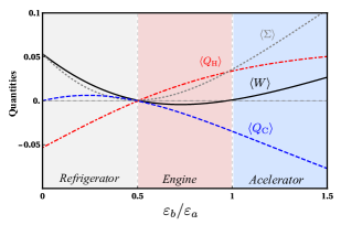
Figure 1: Thermodynamics quantities for the two-stroke quantum machine. Averages of the extracted work $\langle W_{\text{net}}\rangle$ (black solid line), released heat by the hot bath $\langle Q_{\text{hot}}\rangle$ (red dash-dotted line), cold heat $\langle Q_{\text{cold}}\rangle$ (blue dashed line) and entropy production $\langle\Sigma\rangle$ (gray dotted line) as a function of $\varepsilon_{b}/\varepsilon_{a}$. We considered the following set of parameters: $\varepsilon_{a}=1$, $\varepsilon_{b}=2\varepsilon_{a}$, $\beta_{a}=1$, $\beta_{b}=2\beta_{a}$, $\kappa=1$, $\Omega=10\kappa$ and $t=\kappa$.

IV Two-stroke heat engine

The two-stroke quantum cycle is engendered as follows: First stroke - The two qubits, initially prepared in local thermal states, are detached from the local thermal baths and put in contact to interact with each other through the nonlinear spin squeezing operation, with the Hamiltonian given by Eq. (2). During the time evolution, the two qubits become quantum correlated, and spin squeezing is generated. Moreover, due to the switch-on of nonlinear interaction, work can be performed on or extracted from the system in this stroke.

Second stroke - The two qubits interact with their respective local thermal reservoirs, releasing or absorbing heat from them depending on the set of parameters employed.

In a two-stroke heat engine, the thermodynamic quantities, i.e., the hot absorbed and released from/to the thermal reservoirs, the extracted work, and the total entropy production, characterizing the cycle become

$$\langle Q_{\text{hot}}\rangle = -\Delta E_{1}=-\left(E_{1}\left(\tau\right)-E_{1}\left(0\right)\right),$$ (3)

$$\langle Q_{\text{cold}}\rangle=-\Delta E_{2}=-\left(E_{2}\left(\tau\right)-E_{2}\left(0\right)\right),$$ (4)

$$\langle W_{\text{net}}\rangle=-\langle Q_{\text{hot}}\rangle-\langle Q_{\text{cold}}\rangle,$$ (5)

$$\langle\Sigma\rangle=-\beta_{1}\langle Q_{\text{hot}}\rangle-\beta_{2}\langle Q_{\text{cold}}\rangle,$$ (6)

with $E_{i}\left(t\right)=\text{Tr$\left[\mathcal{H}_{t}\rho_{i}\left(t\right)\right]$}$. We use the characteristic function approach to obtain all nonequilibrium thermodynamic quantities outlined in Eq. (3-6) (see more details in Appendix B). For the engine operation, we have to ensure the conditions $\langle Q_{\text{hot}}\rangle>0$, $\langle Q_{\text{cold}}\rangle<0$, and $\langle W_{\text{net}}\rangle<0$, while the entropy production is always positive, as illustrated in Fig. 1, regardless of the cycle configuration, according to the second law of thermodynamics $\langle\Sigma\rangle\geq 0$. To quantify the engine performance, we use as figures of merit the efficiency and extracted power, defined as $\eta=-\langle W_{\text{net}}\rangle/\langle Q_{\text{hot}}\rangle$ and $\mathcal{P}=-\langle W_{\text{net}}\rangle/t$, respectively, where $t$ represents the interaction time.

V Results

We begin our investigation of the quantum engine by examining the spin squeezing generated during this mode of operation. From Eq. (2) it is clear that the nonlinear feature of the engine is dictated by the intensity of the parameter $\kappa$. With this in mind, Fig. 2-(a) depicts the Kitagawa and Ueda’s spin squeezing parameter as a function of the interaction time for different values of nonlinear parameter $\kappa$, to show how the parameter $\xi$ depends on interaction time. We observe that due to the orthogonal contribution, encoded in the parameter $\Omega$, turned on during our analysis, the intensity of the spin squeezing in the engine regime is attenuated to some values of the interaction time. The choice in the specific range of time interaction is appropriated to ensure the engine regime as displayed in Fig. 1.

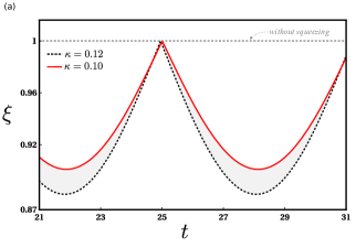
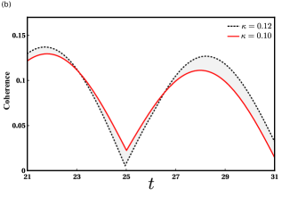
Figure 2: (a) Spin squeezing parameter $\xi$ as a function of the interaction time for different values of nonlinear parameter: $\kappa=0.12$ (black dashed line), $\kappa=0.10$ (red solid line). (b) $l_{1}$-norm of coherence as a function of $t$ to quantify the global coherence in the energy basis. In both cases, we consider the following set of parameters: $\beta_{a}=1$, $\beta_{b}=2\beta_{A}$, $\varepsilon_{a}=1$, $\varepsilon_{b}=0.6\varepsilon_{a}$ and $\Omega=0.5$.

Likewise, in Fig. 2-(b), we show how spin squeezing is directly associated with the production of coherence in the global basis of the system, which in turn, is a signature of quantum correlation [67]. In Fig. 2-(b) we show the $l_{1}$-norm to quantify the dynamics of coherence in the global basis (energy basis) of the two spins. Notice that, the coherence dynamics during the engine regime is directly linked to the spin squeezing produced by the nonlinear interaction. Specifically, the maximum values of the coherence match with the maximums of the spin squeezing parameter and vice versa. This highlights the role played by the term $\kappa$ in the nonlinear Hamiltonian in Eq. (2), by controlling the amount of coherence generated in the first stroke.

We now turn our attention to the thermodynamics and performance of the two-stroke quantum heat engine and spin squeezing effects. From the thermodynamic quantities, obtained through the characteristic function (see details in Appendix B), and choosing the appropriated relation between the two frequencies $\varepsilon_{a}$ and $\varepsilon_{b}$ such that the cycle operates as an engine (see Fig. 1) the figures of merit as efficiency and extracted power can be analyzed.

Figure 3-(a) and 3-(b) illustrate the behavior of efficiency and extracted power as a function of the interaction time for two values of the nonlinear parameter $\kappa$, respectively. For clarity, in Fig. 3-(a) we also indicate the Otto and Carnot efficiencies for the parameters considered. The oscillatory behavior in both efficiency and extracted power is clearly due to the introduction of the spin squeezing effects in the system Hamiltonian, whereas the intensity of it depends on the value of $\kappa$. We observe that irrespective of the value of $\kappa$, it is possible to reach the Otto efficiency provided a sufficiently high control over the systems parameter, i.e., the intensity of the spin squeezing and the squeezing operation time. Figure 3-(b) illustrates the fact that the maximum value of the extracted power follows that of the efficiency. Both of them are in agreement with the minimum value of spin squeezing or coherence, Fig. 2.

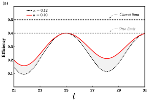
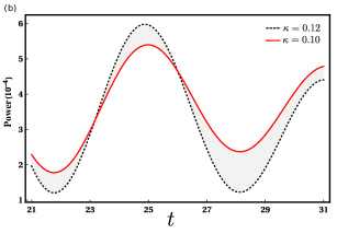
Figure 3: (a) Efficiency and (b) extracted power of the two-stroke quantum heat engine as a function of the interaction time for different values of nonlinear parameter: $\kappa=0.12$ (black dashed line), $\kappa=0.10$ (red solid line). We have considered the same set of parameters as in Fig. 2.

The total entropy production $\langle\Sigma\rangle$ along the cycle is also a relevant thermodynamic quantity once it amounts to the degree of irreversibility in a general process or cycle [2, 68]. By using the characteristic function we can express exactly the total entropy production for the engine cycle as in Eq. (34). Figure 4 depicts the total entropy production for the engine cycle as a function of the interaction time for two values of $\kappa$. Again, the spin squeezing effect introduces the oscillatory behavior and we observe that the minimum entropy production value coincides with the maximum efficiency for the cycle, in agreement with the general result in Ref. [19]. We highlight that a suitable value for the total entropy production may be achieved provided a high control over the experimental parameters.

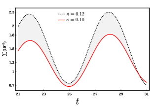
Figure 4: Total entropy production as a function of the interaction time for different values of nonlinear parameter: $\kappa=0.12$ (black dashed line), $\kappa=0.10$ (red solid line). We consider the same set of parameters displayed in Fig. 2.

VI Conclusion

We have theoretically investigated a quantum thermal machine model where spin squeezing interaction is intrinsically considered in the system. First, we verified that by changing the energy gap ratio between the two qubits it is possible to operate the cycle in a refrigerator, engine, or accelerator regime. We have chosen the engine configuration to study the relation between the performance and spin squeezing degree. To quantify the degree of spin squeezing during the cycle dynamics, we employed Kitagawa and Ueda’s parameter and we show that the coherent amount is linked to the spin squeezing parameter.

All thermodynamic quantities to characterize the engine performance were evaluated through the characteristic formalism. The performance of the engine was studied through the efficiency and extracted power. We verified that the more the amount of spin squeezing in a given time, the less the efficiency and extracted power. Thus, for a cycle in which the spin squeezing operation is always on, the best performance may be achieved provided a high control over the parameters. We also considered the irreversibility of the cycle by computing the total entropy production. The results indicate that the more the spin squeezing degree, the more the total entropy production in a cycle. This aspect is associated with the performance of the engine for a given value of the interaction time. We hope that this work can contribute to unveiling the role played by quantum correlations in nontrivial quantum thermal machines. Finally, our model also allows for experimental implementation, for instance, in nuclear magnetic resonance.

Appendix A Kitagawa and Ueda’s parameter

In the section, we explicit the Eq. (1) for a quantum initial state, $\rho_{0}$, which has the mean spin direction (MSD) $\vec{n}_{0}$ in the $z$ direction

$$\vec{n}_{0}=\frac{\langle{\mathcal{S}}\rangle}{|\langle\mathcal{S}\rangle|}=\frac{\mathcal{S}_{z}}{|\langle\mathcal{S}\rangle|}.$$ (7)

After the interaction with one kind of nonlinear Hamiltonian the final state, $\rho_{t}=\mathcal{U}(t)\rho_{0}\mathcal{U}^{\dagger}(t)$, may have its fluctuation reduced in some direction. Since the MSD is in the $z$ direction, we can introduce an orthogonal vector as $\vec{n}_{\perp}=x\cos(\phi)+y\sin(\phi)$ and therefore the spin component becomes

$$\mathcal{S}_{n_{\perp}}=\mathcal{S}_{x}\cos(\phi)+\mathcal{S}_{y}\sin(\phi),$$ (8)

where $\phi$ is an arbitrary angle belonging to the xy-plane. In turn, for this particular initial state, we have that the variance is equal to $\Delta\mathcal{S}_{n_{\perp}}^{2}=\langle\mathcal{S}_{n_{\perp}}^{2}\rangle$, since the average are $\langle\mathcal{S}_{x}\rangle=\langle\mathcal{S}_{y}\rangle=0$. Thereby, the variance of the spin component in the orthogonal direction for the final state $\rho_{t}$ becomes

$$\left(\Delta\mathcal{S}_{n_{\perp}}^{2}\right) =\frac{1}{2}\langle\mathcal{S}_{x}^{2}+\mathcal{S}_{y}^{2}\rangle+\frac{1}{2}\langle\mathcal{S}_{x}^{2}-\mathcal{S}_{y}^{2}\rangle\cos(2\phi)$$

$$+\frac{1}{2}\sin(2\phi)\langle\left\{\mathcal{S}_{x},\mathcal{S}_{y}\right\}\rangle,$$ (9)

where we used the anti-commutator term $\left\{\mathcal{S}_{x},\mathcal{S}_{y}\right\}=\mathcal{S}_{x}\mathcal{S}_{y}+\mathcal{S}_{y}\mathcal{S}_{x}$ and trigonometric relations. As shown in Eq. (9), the variance $\Delta\mathcal{S}_{n_{\perp}}^{2}$ is a function of the angle $\phi$ and therefore its minimization can be obtained through the derivation of the equation concerning this angle providing the following reduced variance

$$\delta_{-}=\frac{1}{2}\left[\langle\mathcal{S}_{x}^{2}+\mathcal{S}_{y}^{2}\rangle-\sqrt{\langle\mathcal{S}_{x}^{2}-\mathcal{S}_{y}^{2}\rangle^{2}+\langle\left\{\mathcal{S}_{x},\mathcal{S}_{y}\right\}\rangle^{2}}\right],$$ (10)

where $\delta_{-}\equiv\left(\Delta\mathcal{S}_{n_{\perp}}^{2}\right)_{\text{min}}$ corresponding the squeezing along the orthogonal direction $\vec{n}_{\perp}$ with the respective optimally squeezing angle

$$\phi_{\text{opt}}=\frac{\pi}{2}+\frac{1}{2}\arctan\left[\frac{\langle\left\{\mathcal{S}_{x},\mathcal{S}_{y}\right\}\rangle^{2}}{\langle\mathcal{S}_{x}^{2}-\mathcal{S}_{y}^{2}\rangle}\right].$$ (11)

Therefore, using the Eq. (10), the Kitagawa and Ueda’s parameter, Eq. (1), for an initial state, $\rho_{0}$, belonging to the $z$-direction becomes

$$\xi=\alpha_{1}-\sqrt{\alpha_{2}+\alpha_{3}},$$ (12)

with,

$$\alpha_{1}=\frac{2\langle\mathcal{S}_{x}^{2}+\mathcal{S}_{y}^{2}\rangle}{N},$$ (13)

$$\alpha_{2}=\frac{4\langle\mathcal{S}_{x}^{2}-\mathcal{S}_{y}^{2}\rangle^{2}}{N^{2}},$$ (14)

$$\alpha_{3}=\frac{4\langle\left\{\mathcal{S}_{x},\mathcal{S}_{y}\right\}\rangle^{2}}{N^{2}}.$$ (15)

Note that the Eq. (12) strongly depends on the expected values $\langle\mathcal{S}_{x}^{2}\rangle,\langle\mathcal{S}_{y}^{2}\rangle$, $\langle\left\{\mathcal{S}_{x},\mathcal{S}_{y}\right\}\rangle^{2}$ and although those do not appear explicitly all quantities depend on the interaction time with the nonlinear Hamiltonian [54, 55, 56].

In our case, the Kitagawa and Ueda’s parameter, Eq. (12), for the final state $\rho_{t}=\mathcal{U}_{t}\rho_{0}\mathcal{U}_{t}^{\dagger}$, with $\mathcal{U}_{t}=\exp[-i\mathcal{H}t]$ and $\rho_{0}=\zeta_{T_{1}}^{th}\otimes\zeta_{T_{2}}^{th}$ is given by

$$\xi=1-\frac{\kappa\mathcal{Z}\Lambda}{\gamma^{2}}|\sin(\gamma t/2)|,$$ (16)

with

$$\mathcal{Z}=1-\frac{1}{\mathcal{Z}_{b}}-\frac{1}{\mathcal{Z}_{a}},$$ (17)

$$\gamma=\sqrt{4\Omega^{2}+\kappa^{2}},$$ (18)

and

$$\Lambda=\sqrt{16\Omega^{2}+2\kappa^{2}[1+\cos(\gamma t)]}.$$ (19)

Therefore, it is straight to see from Eq. (16) that when the nonlinear parameter is zero, i.e., $\kappa=0$, there is no spin squeezing, $\xi=1$.

Appendix B Characteristic function and thermodynamic quantities

To study the thermodynamics quantities along the cycle, we employ the characteristic function, $\chi(\lambda,\mu)$, which allows us to obtain all moments associated with the random variables. According to the two-point measurement protocol, we can jointly estimate work and heat by the characteristic function as follows [69, 70]

$$\chi(\lambda,\nu) =$$ (20)

$$\text{Tr}\left[\mathcal{U}_{t}^{\dagger}e^{i(\lambda-\nu)\mathcal{H}_{a}}e^{i\lambda\mathcal{H}_{b}}\mathcal{U}_{t}e^{-i(\lambda-\nu)\mathcal{H}_{a}}e^{-i\lambda\mathcal{H}_{b}}\rho_{0}\right].$$

Using the characteristic function, Eq.(20), we can obtain all moments associated with the random variables ($W_{\text{net}}$) and ($Q_{\text{hot}}$) by the relation

$$\langle W^{n}_{\text{net}}Q_{\text{hot}}^{m}\rangle=(-i)^{n+m}\frac{\partial^{n+m}\chi(\lambda,\nu)}{\partial^{n}\lambda\partial^{m}\nu}\rvert_{{}_{\lambda=0,\nu=0}},$$ (21)

as well as the entropy production

$$\langle\Sigma\rangle=(\beta_{b}-\beta_{a})\langle Q_{\text{hot}}\rangle+\beta_{b}\langle W_{\text{net}}\rangle,$$ (22)

and the cold hot

$$\langle Q_{\text{cold}}\rangle=-\langle W_{\text{net}}\rangle-\langle Q_{\text{hot}}\rangle.$$ (23)

Before providing explicit details on the characteristic function and nonequilibrium thermodynamics quantities, we show how the unitary evolution matrix that describes the nonlinear Hamiltonian Eq. (2) reads

$$\mathcal{U}_{t}=e^{-i\mathcal{H}t}=\left(\begin{array}[]{cccc}u_{11}&0&0&u_{14}\\ 0&u_{22}&u_{23}&0\\ 0&u_{23}&u_{22}&0\\ u_{14}&0&0&u_{44}\end{array}\right),$$ (24)

with the following matrix elements

$$u_{11}=e^{-i\kappa t/2}\left[\cos\left(\gamma t/2\right)-i\frac{2\Omega}{\gamma}\sin\left(\gamma t/2\right)\right],$$ (25)

$$u_{44}=e^{-i\kappa t/2}\left[\cos\left(\gamma t/2\right)+i\frac{2\Omega}{\gamma}\sin\left(\gamma t/2\right)\right],$$ (26)

$$u_{14}=-\frac{i\kappa}{\gamma}e^{-i\kappa t/2}\sin\left(\gamma t/2\right),$$ (27)

$$u_{22}=\frac{1}{2}\left[e^{-i\kappa t/2}+1\right],$$ (28)

$$u_{23}=\frac{1}{2}\left[e^{-i\kappa t/2}-1\right].$$ (29)

Substituting the individual Hamiltonians for each qubit $\mathcal{H}_{i}=-\varepsilon_{i}\sigma_{z}/2$ where $i\in\{a,b\}$ and the unitary matrix Eq. (24) in the Eq. (20) ones can explicitly obtain the characteristics function

$$\chi(\lambda,\nu) =\frac{1}{\mathcal{Z}_{a}\mathcal{Z}_{b}}|u_{11}|^{2}\left(1+e^{\beta_{a}\varepsilon_{a}+\beta_{b}\varepsilon_{b}}\right)$$

$$+\frac{1}{\mathcal{Z}_{a}\mathcal{Z}_{b}}|u_{22}|^{2}\left(e^{\beta_{a}\varepsilon_{a}}+e^{\beta_{b}\varepsilon_{b}}\right)$$

$$+\frac{1}{\mathcal{Z}_{a}\mathcal{Z}_{b}}|u_{14}|^{2}e^{-i\varepsilon_{a}(\lambda-\mu)-i\lambda\varepsilon_{b}}$$

$$+\frac{1}{\mathcal{Z}_{a}\mathcal{Z}_{b}}|u_{14}|^{2}e^{i\varepsilon_{a}(\lambda-\mu)+i\lambda\varepsilon_{b}}e^{\beta_{a}\varepsilon_{a}+\beta_{b}\varepsilon_{b}}$$

$$+\frac{1}{\mathcal{Z}_{a}\mathcal{Z}_{b}}|u_{23}|^{2}e^{i\varepsilon_{a}(\lambda-\mu)-i\lambda\varepsilon_{b}}e^{\beta_{a}\varepsilon_{a}}$$

$$+\frac{1}{\mathcal{Z}_{a}\mathcal{Z}_{b}}|u_{23}|^{2}e^{-i\varepsilon_{a}(\lambda-\mu)+i\lambda\varepsilon_{b}}e^{\beta_{b}\varepsilon_{b}}.$$ (30)

Note that the matrix elements of the interaction are essential to evaluate the characteristic function. In turn, we can explore the Eq. (21-23) to obtain the nonequilibrium thermodynamic quantities

$$\langle W_{\mathrm{net}}\rangle =\frac{\kappa^{2}(\varepsilon_{a}+\varepsilon_{b})}{\gamma^{2}\mathcal{Z}_{a}\mathcal{Z}_{b}}\sin^{2}\left(\gamma t/2\right)\left(e^{\beta_{a}\varepsilon_{a}+\beta_{b}\varepsilon_{b}}-1\right)$$

$$+\frac{\left(1-\cos\left(\kappa t\right)\right)(\varepsilon_{a}-\varepsilon_{b})}{2\mathcal{Z}_{a}\mathcal{Z}_{b}}\left(e^{\beta_{a}\varepsilon_{a}}-e^{\beta_{b}\varepsilon_{b}}\right),$$ (31)

$$\langle Q_{\mathrm{hot}}\rangle =\frac{\kappa^{2}\varepsilon_{a}}{\gamma^{2}\mathcal{Z}_{a}\mathcal{Z}_{b}}\sin^{2}\left(\gamma t/2\right)\left(1-e^{\beta_{a}\varepsilon_{a}+\beta_{b}\varepsilon_{b}}\right)$$

$$-\frac{\varepsilon_{a}\left(1-\cos\left(\kappa t\right)\right)}{2\mathcal{Z}_{a}\mathcal{Z}_{b}}\left(e^{\beta_{a}\varepsilon_{a}}-e^{\beta_{b}\varepsilon_{b}}\right),$$ (32)

$$\langle Q_{\mathrm{cold}}\rangle =\frac{\kappa^{2}\varepsilon_{b}}{\gamma^{2}\mathcal{Z}_{a}\mathcal{Z}_{b}}\sin^{2}\left(\gamma t/2\right)\left(1-e^{\beta_{a}\varepsilon_{a}+\beta_{b}\varepsilon_{b}}\right)$$

$$+\frac{\varepsilon_{b}\left(1-\cos\left(\kappa t\right)\right)}{2\mathcal{Z}_{a}\mathcal{Z}_{b}}\left(e^{\beta_{a}\varepsilon_{a}}-e^{\beta_{b}\varepsilon_{b}}\right),$$ (33)

$$\langle\Sigma\rangle= \frac{\kappa^{2}\sin^{2}(\gamma t/2)(\beta_{a}\varepsilon_{a}+\beta_{b}\varepsilon_{b})}{\gamma^{2}\mathcal{Z}_{a}\mathcal{Z}_{b}}\left(e^{\beta_{a}\varepsilon_{a}+\beta_{b}\varepsilon_{b}}-1\right)$$

$$+ \frac{\left(1-\cos(\kappa t)\right)(\beta_{a}\varepsilon_{a}-\beta_{b}\varepsilon_{b})}{2\mathcal{Z}_{a}\mathcal{Z}_{b}}\left(e^{\beta_{a}\varepsilon_{a}}-e^{\beta_{b}\varepsilon_{b}}\right).$$ (34)

References

- [1] A. Auffèves, Quantum Technologies Need a Quantum Energy Initiative, PRX Quantum 3, 020101 (2022).
- [2] G. T. Landi and M. Paternostro, Irreversible entropy production: From classical to quantum, Rev. Mod. Phys. 93, 035008 (2021).
- [3] R. Kosloff, Quantum thermodynamics: A dynamical viewpoint, Entropy 15, 2100 (2013).
- [4] F. Binder, L. A. Correa, C. Gogolin, J. Anders, and G. Adesso, eds., Thermodynamics in the Quantum Regime: Fundamental Aspects and New Directions (Springer International, Cham, Swtizerland, 2018).
- [5] J. Goold, M. Huber, A. Riera, L. del Rio, and P. Skrzypczyk, The role of quantum information in thermodynamics a topical review, J. Phys. A: Math. Theor. 49, (2016) 143001.
- [6] S. Deffner and S. Campbell, Quantum Thermodynamics An Introduction to the Thermodynamics of Quantum Information (Morgan & Claypool, San Rafael, CA, 2019).
- [7] M. Campisi, P. Hänggi, and P. Talkner, Quantum fluctuation relations: Foundations and applications, Rev. Mod. Phys. 83, 771 (2011).
- [8] M. Esposito, U. Harbola, and S. Mukamel, Nonequilibrium fluctuations, fluctuation theorems, and counting statistics in quantum systems, Rev. Mod. Phys. 81, 1665 (2009).
- [9] N. M. Myers, O. Abah, and S. Deffner, Quantum thermodynamic devices: From theoretical proposals to experimental reality, AVS Quantum Sci. 4, 027101 (2022).
- [10] C. H. S. Vieira and J. L. D. de Oliveira and J. F. G. Santos and P. R. Dieguez and R. M. Serra, Exploring quantum thermodynamics with NMR, J. Magn. Reson. Open 16-17, 100105 (2023).
- [11] S. Vinjanampathy and J. Anders, Quantum Thermodynamics, Contemporary Physics 57, 545 (2016).
- [12] T. B. Batalhão, A. M. Souza, L. Mazzola, R. Auccaise, R. S. Sarthour, I. S. Oliveira, J. Goold, G. De Chiara, M. Paternostro, and R. M. Serra, Experimental reconstruction of work distribution and study of fluctuation relations in a closed quantum system, Phys. Rev. Lett. 113, 140601 (2014).
- [13] Y. Chu and J. Cai, Thermodynamic Principle for Quantum Metrology, Phys. Rev. Lett. 128, 200501 (2022).
- [14] H.-G. Xu, J. Jin, G. D. M. Neto, and N. G. de Almeida, Universal quantum Otto heat machine based on the Dicke model, Phys. Rev. E 109, 014122 (2024)
- [15] H. T. Quan, Yu-xi Liu, C. P. Sun, and F. Nori, Quantum thermodynamic cycles and quantum heat engines, Phys. Rev. E 76, 031105 (2007).
- [16] Y. Xiao, D. Liu, J. He, Y. Ma, Z. Wu, and J. Wang, Quantum Otto engine with quantum correlations, Phys. Rev. A 108, 042614 (2023).
- [17] F. Altintas, A. U. C. Hardal, Ozgur E. Mustecaplıoglu, Quantum correlated heat engine with nonlinear spin-spin interactions, Phys. Rev. E 90, 032102 (2014).
- [18] M. Asadian, S. Ahadpour, and F. Mirmasoudi, Quantum correlated heat engine in XY chain with Dzyaloshinskii–Moriya interactions, Sci Rep 12, 7081 (2022).
- [19] P. A. Camati, J. F. G. Santos, and R. M. Serra, Coherence effects in the performance of the quantum Otto heat engine. Phys. Rev. A 99, 062103 (2019).
- [20] J. P. S. Peterson, T. B. Batalhão, M. Herrera, A. M. Souza, R. S. Sarthour, I. S. Oliveira, and R. M. Serra, Experimental characterization of a spin quantum heat engine. Phys. Rev. Lett. 123, 240601 (2019).
- [21] Z. Lin, S. Su, J. Chen, J. Chen, and J. F. G. Santos, Suppressing coherence effects in quantum-measurement-based engines, Phys. Rev. A 104, 062210 (2021).
- [22] G. Manzano, Squeezed thermal reservoir as a generalized equilibrium reservoir, Phys. Rev. E 98, 042123 (2018).
- [23] J. Klaers, S. Faelt, A. Imamoglu, and E. Togan, Squeezed Thermal Reservoirs as a Resource for a Nanomechanical Engine beyond the Carnot Limit, Phys. Rev. X 7, 031044 (2017).
- [24] R. J. de Assis, J. S. Sales, J. A. R. da Cunha, and N. G. de Almeida, Universal two-level quantum Otto machine under a squeezed reservoir, Phys. Rev. E 102, 052131 (2020).
- [25] R. J de Assis, J. S Sales, U. C Mendes and N. G de Almeida, Two-level quantum Otto heat engine operating with unit efficiency far from the quasi-static regime under a squeezed reservoir, J. Phys. B: At. Mol. Opt. Phys. 54 095501 (2021).
- [26] J. Rossnagel, O. Abah, F. Schmidt-Kaler, K. Singer, and E. Lutz, Nanoscale Heat Engine beyond the Carnot Limit, Phys. Rev. Lett. 112, 030602 (2014).
- [27] O. Abah and E. Lutz, Efficiency of heat engines coupled to nonequilibrium reservoirs, Eur. Phys. Lett. 106 20001 (2014).
- [28] J. F G Santos and F. S. Luiz, Quantum thermodynamics aspects with a thermal reservoir based on -symmetric Hamiltonians, J. Phys. A: Math. Theor. 54 335301 (2021).
- [29] J. F. G. Santos and P. Chattopadhyay, -symmetric effects in measurement-based quantum thermal machines, Physica A 632, 129342 (2023).
- [30] Experimental investigation of a quantum heat engine powered by generalized measurements, V. F. Lisboa, P. R. Dieguez, J. R. Guimarães, J. F. G. Santos, and R. M. Serra, Phys. Rev. A 106, 022436 (2022).
- [31] L. Bresque, P. A. Camati, S. Rogers, K. Murch, A. N. Jordan, and A. Auffèves, Two-Qubit Engine Fueled by Entanglement and Local Measurements, Phys. Rev. Lett. 126, 120605 (2021).
- [32] L. Buffoni, A. Solfanelli, P. Verrucchi, A. Cuccoli, and M. Campisi, Quantum Measurement Cooling, Phys. Rev. Lett. 122, 070603 (2019).
- [33] X. Ding, J. Yi, Y. W. Kim, and P. Talkner, Measurement-driven single temperature engine, Phys. Rev. E 98, 042122 (2018).
- [34] A. Jordan, C. Elouard, and A. Auffèves, Quantum measurement engines and their relevance for quantum interpretations, Quantum Stud. Math. Found. 7, 203 (2020).
- [35] P. A. Camati, J. F. G. Santos, and R. M. Serra, Employing non-Markovian effects to improve the performance of a quantum Otto refrigerator, Phys. Rev. A 102, 012217 (2020).
- [36] K. Ptaszynski, Non-Markovian thermal operations boosting the performance of quantum heat engines, Phys. Rev. E 106, 014114 (2022).
- [37] F Cavaliere, M. Carrega, G. De Filippis, V. Cataudella, G. Benenti, and M. Sassetti, Dynamical heat engines with non-Markovian reservoirs, Phys. Rev. Research 4, 033233 (2022).
- [38] G. De Chiara and M. Antezza, Quantum machines powered by correlated baths, Phys. Rev. Research 2, 033315 (2020).
- [39] J. Yi, P. Talkner, and Y. W. Kim, Single-temperature quantum engine without feedback control, Phys. Rev. E 96, 022108 (2017).
- [40] M. H. Mohammady and J. Anders, A quantum Szilard engine without heat from a thermal reservoir, New J. Phys. 19, 113026 (2017).
- [41] C. Elouard, D. Herrera-Martí, B. Huard, and A.Auffèves, Extracting Work from Quantum Measurement in Maxwell’s Demon Engines, Phys. Rev. Lett. 118, 260603 (2017).
- [42] K. Brandner, M. Bauer, M. T. Schmid and U. Seifert, Coherence-enhanced efficiency of feedback-driven quantum engines, New J. Phys. 17, 065006 (2015).
- [43] A. M. Timpanaro, G. Guarnieri, J. Goold, and G. T. Landi, Thermodynamic Uncertainty Relations from Exchange Fluctuation Theorems, Phys. Rev. Lett. 123, 090604 (2019).
- [44] M. F. Sacchi, Thermodynamic uncertainty relations for bosonic Otto engines, Phys. Rev. E 103, 012111 (2021).
- [45] M. Herrera, J. H. Reina, I. D’Amico, and R. M. Serra, Correlation-boosted quantum engine: A proof-of-principle demonstration, Phys. Rev. Research 5, 043104 (2023).
- [46] A. Sorensen, L. Duan, J. Cirac, and P. Zoller, Many-particle entanglement with Bose-Einstein condensates, Nature 409, 63 (2001).
- [47] O. Guehne and G. Toth, Entanglement detection, Phys. Rep. 474, 1 (2009).
- [48] L. Amico, R. Fazio, A. Osterloh, and V. Vedral, Entanglement in many-body systems, Rev. Mod. Phys. 80, 517 (2008).
- [49] D. J. Wineland, J. J. Bollinger, W. M. Itano, F. L. Moore, D. J. Heinzen, Spin squeezing and reduced quantum noise in spectroscopy, Phys. Rev. A 46, R6797(R) (1992).
- [50] L. Pezze, A. Smerzi, Entanglement, nonlinear dynamics, and the Heisenberg limit, Phys. Rev. Lett. 102 100401 (2009).
- [51] J.M. Robinson, M. Miklos, Y.M. Tso et al, Direct comparison of two spin-squeezed optical clock ensembles at the level, Nat. Phys. (2024).
- [52] R. Kaubruegger, P. Silvi, C. Kokail, R. van Bijnen, A. M. Rey, J. Ye, A. M. Kaufman, and P. Zoller, Variational spin squeezing Algorithms on Programmable Quantum Sensors, Phys. Rev. Lett. 123, 260505 (2019).
- [53] B. Lu, L. Liu, J.-Y. Song, K. W. C. Wang, Recent progress on coherent computation based on quantum squeezing, AAPPS Bull. 33, 7 (2023).
- [54] J. Ma, X. Wang, C. Sun, and F. Nori, Quantum spin squeezing, Phys. Rep. 509, 89 (2011).
- [55] M. Kitagawa and M. Ueda, Squeezed spin states, Phys. Rev. A 47, 5138 (1993).
- [56] X. Wang and B. C. Sanders, Spin squeezing and pairwise entanglement for symmetric multiqubit states, Phys. Rev. A 68, 012101 (2003).
- [57] E. Yukawa, G. J. Milburn, C. A. Holmes, M. Ueda, and K. Nemoto, Precision measurements using squeezed spin states via two-axis countertwisting interactions, Phys. Rev. A 90, 062132 (2014).
- [58] D. Kajtoch and E. Witkowska, Quantum dynamics generated by the two-axis countertwisting Hamiltonian, Phys. Rev. A 92, 013623 (2015).
- [59] T. Fernholz, H. Krauter, K. Jensen, J. F. Sherson, A. S. Sorensen, and E. S. Polzik, Spin squeezing of atomic ensembles via nuclear-electronic spin entanglement, Phys. Rev. Lett. 101, 073601 (2008).
- [60] M. Takeuchi, S. Ichihara, T. Takano, M. Kumakura, T. Yabuzaki, and Y. Takahashi, Spin squeezing via one-axis twisting with coherent light, Phys. Rev. Lett. 94, 023003 (2005).
- [61] Sinha, S., Emerson, J., Boulant, N. et al., Experimental Simulation of Spin Squeezing by Nuclear Magnetic Resonance, Quantum Information Processing 2, 433–448 (2003).
- [62] C. K. Law, H. T. Ng, and P. T. Leung, Coherent control of spin squeezing, Phys. Rev. A 63, 055601 (2001).
- [63] F. Altintas, A. Ü. C. Hardal, Ö. E. Müstecaplıoglu, Quantum correlated heat engine with spin squeezing, Phys. Rev. E 90, 032102 (2014).
- [64] G. J. Milburn and J. Corney, Quantum dynamics of an atomic Bose-Einstein condensate in a double-well potential, Phys. Rev. A 55, 4318 (1997).
- [65] D. Jaksch, J. Cirac, P. Zoller, Dynamically turning off interactions in a two-component condensate, Phys. Rev. A 65 033625 (2002).
- [66] H. Jing, Mutual coherence and spin squeezing in double-well atomic condensates, Phys. Lett. A 306 (2002).
- [67] T. Baumgratz, M. Cramer and M. B. Plenio, Quantifying Coherence, Phys. Rev. Lett. 113, 140401 (2014).
- [68] Santos, J.P., Céleri, L.C., Landi, G.T. et al., The role of quantum coherence in nonequilibrium entropy production, npj Quantum Inf 5, 23 (2019).
- [69] M. Esposito and C. Van den Broeck, Three Detailed Fluctuation Theorems, Phys. Rev. Lett. 104, 090601 (2010).
- [70] M F. Sacchi, Thermodynamic uncertainty relations for bosonic Otto engines, Phys. Rev. E 103, 012111 (2021).