Score-based Causal Representation Learning:
Linear and General Transformations

Abstract

This paper addresses intervention-based causal representation learning (CRL) under a general nonparametric latent causal model and an unknown transformation that maps the latent variables to the observed variables. Linear and general transformations are investigated. The paper addresses both the identifiability and achievability aspects. Identifiability refers to determining algorithm-agnostic conditions that ensure recovering the true latent causal variables and the latent causal graph underlying them. Achievability refers to the algorithmic aspects and addresses designing algorithms that achieve identifiability guarantees. By drawing novel connections between score functions (i.e., the gradients of the logarithm of density functions) and CRL, this paper designs a score-based class of algorithms that ensures both identifiability and achievability. First, the paper focuses on linear transformations and shows that one stochastic hard intervention per node suffices to guarantee identifiability. It also provides partial identifiability guarantees for soft interventions, including identifiability up to ancestors for general causal models and perfect latent graph recovery for sufficiently non-linear causal models. Secondly, it focuses on general transformations and shows that two stochastic hard interventions per node suffice for identifiability. Notably, one does not need to know which pair of interventional environments have the same node intervened.

Keywords: causal representation learning, causality, interventions

1 Overview

Causal representation learning (CRL) aims to form a causal understanding of the world by learning appropriate representations that support causal interventions, reasoning, and planning (Schölkopf et al., 2021). Specifically, CRL considers a data-generating process in which high-level latent causally-related variables are mapped to low-level, generally high-dimensional observed data through an unknown transformation. Formally, consider a causal Bayesian network (Pearl, 2009) encoded by a directed acyclic graph (DAG) $\mathcal{G}$ with $n$ nodes and generating causal random variables $Z\triangleq[Z_{1},\dots,Z_{n}]^{\top}$. These random variables are transformed by an unknown function $g:{\mathbb{R}}^{n}\to{\mathbb{R}}^{d}$ to generate the $d$-dimensional observed random variables $X\triangleq[X_{1},\dots,X_{d}]^{\top}$ according to:

$$X=g(Z)\ .$$ (1)

CRL is the process of using the observed data $X$ and recovering (i) the causal structure $\mathcal{G}$ and (ii) the latent causal variables $Z$. Achieving these implicitly involves another objective of recovering the unknown transformation $g$ as well. Addressing CRL consists of two central questions:

• Identifiability, which refers to determining the necessary and sufficient conditions under which $\mathcal{G}$ and $Z$ can be recovered. The scope of identifiability (e.g., perfect or partial) critically depends on the extent of information available about the data, the underlying causal structure, and the transformation. The nature of the identifiability results is generally algorithm-agnostic and can be non-constructive without specifying how to recover $\mathcal{G}$ and $Z$.

• Achievability, which complements identifiability and pertains to designing algorithms that can recover $\mathcal{G}$ and $Z$ while maintaining identifiability guarantees. Achievability hinges on forming reliable estimates for the transformation $g$.

CRL from Interventions.

Identifiability is known to be impossible without additional supervision or sufficient statistical diversity among the samples of the observed data $X$. As shown in (Hyvärinen and Pajunen, 1999; Locatello et al., 2019), this is the case even for the simpler settings in which the latent variables are statistically independent (i.e., graph $\mathcal{G}$ has no edges). Interventions are effective mechanisms for introducing proper statistical diversity for the models of the observed data. Specifically, an intervention on a set of causal variables alters the causal mechanisms that generate those variables. Note that these causal mechanisms capture the effect of parents on the child variable. Such interventions, even when imposing sparse changes in the statistical models, create variations in the observed data sufficient for learning latent causal representations. This has led to CRL via intervention as an important class of CRL problems, which in its general form has remained an open problem (Schölkopf et al., 2021). This paper addresses this open problem by drawing a novel connection to score functions, i.e., the gradients of the logarithm of density functions.

It is noteworthy that as a form of supervision via interventions, several studies have used counterfactual pairs of observation samples, one collected before and one after an intervention (Ahuja et al., 2022b; Locatello et al., 2020; von Kügelgen et al., 2021; Yang et al., 2021; Brehmer et al., 2022). However, acquiring such data is difficult since it implies being able to directly control the latent representation. Instead, we use a weaker form of supervision via having access to only the pair of distributions before and after an intervention (as opposed to sample pairs). Such supervision is more realistic than access to counterfactual pairs and bodes well for practical applications in genomics (Tejada-Lapuerta et al., 2023) and robotics (Lee et al., 2021).

Contributions.

This paper provides both identifiability and achievability results for CRL from interventions under general latent causal models and general transformations. We establish these results by uncovering hitherto unknown connections between score functions (i.e., the gradients of the logarithm of density functions) and CRL. We leverage these connections to design CRL algorithms that serve as constructive proofs for the identifiability and achievability results. We do not make any parametric assumption on the latent causal model, i.e., the relationships among elements of $Z$ take any arbitrary form. For the transformation $g$, we consider a diffeomorphism (i.e., bijective such that both $g$ and $g^{-1}$ are continuously differentiable) onto its image. Our results are categorized into two main groups based on the form of $g$: (i) linear transformation, and (ii) general (nonparametric) transformation. We consider both stochastic hard and soft interventions, and our contributions are summarized below.

Linear transformations.

We first focus on linear transformations and investigate various extents of identifiability and achievability (perfect and partial) given one intervention per node. In this setting, we consider both hard and soft interventions.

• On identifiability from hard interventions, we show that one hard intervention per node suffices to guarantee perfect identifiability.

• On identifiability from soft interventions, we show that one soft intervention per node suffices to guarantee identifiability up to ancestors – transitive closure of the latent DAG is recovered and latent variables are recovered up to a linear function of their ancestors. Importantly, these results are tight since identifying the latent linear models beyond ancestors using soft interventions is known to be impossible.

• We further tighten the previous result and show that when the latent causal model is sufficiently non-linear, perfect DAG recovery becomes possible using soft interventions. Furthermore, we recover a latent representation that is Markov with respect to the latent DAG, preserving the true conditional independence relationships.

• On achievability, we design an algorithm referred to as Linear Score-based Causal Latent Estimation via Interventions (LSCALE-I). This algorithm achieves the identifiability guarantees under both soft and hard interventions. LSCALE-I consists of modules (i) for achieving identifiability up to ancestors, and (ii) in the case of hard interventions, refines the output of module (i) without requiring any conditional independence test.

General transformations.

In this setting, we do not have any restriction on the transformation from the latent space to the observed space. In this general setting, our contributions are as follows.

• On identifiability, we show that observational data and two distinct hard interventions per node suffice to guarantee perfect identifiability. This result generalizes the recent results in the literature in two ways. First, we do not require the commonly adopted faithfulness assumption on latent causal models. Secondly, we assume the learner does not know which pair of environments intervene on the same node.

• More importantly, on achievability, we design the first provably correct algorithm that recovers $\mathcal{G}$ and $Z$ perfectly. This algorithm is referred to as Generalized Score-based Causal Latent Estimation via Interventions (GSCALE-I). We note that GSCALE-I requires only the score functions of observed variables as its inputs and computes those of the latent variables by leveraging the Jacobian of the decoders.

• We also establish new results that shed light on the role of observational data. Specifically, when two interventional environments per node are given in pairs, observational data is only needed for recovering the latent DAG. Furthermore, we show that observational data can be dispensed with under a weak faithfulness condition on the latent causal model.

Before describing our novel methodology, we recall the general approach to solving CRL. Recovering the latent causal variables hinges on finding the inverse of $g$ based on the observed data $X$, which facilitates recovering $Z$ via $Z=g^{-1}(X)$. In other words, referring to $(g^{-1},g)$ as the true encoder-decoder pair, we search for an encoder that takes observed variables back to the true latent space. A valid encoder should necessarily have an associated decoder to ensure a perfect reconstruction of observed variables from estimated latent variables. However, there are infinitely many valid encoder-decoder pairs that satisfy the reconstruction property. The purpose of using interventions is to inject variations into the observed data, which can help us distinguish among these solutions.

Score-based methodology.

We start by showing that an intervention on a latent node induces changes only in the score function’s coordinates corresponding to the intervened node and its parents. Furthermore, when two interventions on the same node are given, such changes will be limited only to the intervened node (parents intact). This implies that score changes are generally sparse. Furthermore, these score changes contain all the information about the latent causal structure. Motivated by these key properties, we formalize a score-based CRL framework based on which we design provably correct distinct algorithms LSCALE-I and GCALE-I for linear and general transformations, respectively, presented in Section 5. We briefly describe the key technique in GSCALE-I for general transformation via two interventions. LSCALE-I involves more finesse to achieve identifiability using only one intervention per node by exploiting the linearity of the transformation.

Algorithm sketch for general transformations.

Consider two interventional environments in which the same node is intervened. We show that the score functions of the latent variables under these two environments differ only at the coordinate of the intervened node. Subsequently, the key idea is to find an encoder that minimizes the variations in the score functions of the estimated latent variables under said encoder. To this end, we assume that two interventional mechanisms acting on the same node are sufficiently distinct (referred to as interventional discrepancy) so that they provide diversity in information. Subsequently, we show that minimizing the total number of non-zero elements in the score differences of the estimated latent variables finds an encoder that perfectly recovers $\mathcal{G}$ and $Z$. An important process in this methodology is projecting the score changes in observed data to the latent space. We show that this can be done by multiplying the observed score difference by the Jacobian of the decoder. Therefore, recovering $\mathcal{G}$ and $Z$ is facilitated by solving the following problem:

$$\min_{\begin{subarray}{c}{\vspace{0.1in}}\\ {\text{valid}}\\ {\text{enc-dec}}\end{subarray}}\;\;\sum_{\begin{subarray}{c}\text{environment}\\ \text{pairs}\end{subarray}}\Big{\|}\text{Jacobian of decoder}\times\big{(}\text{score differences of $X$}\big{)}\Big{\|}_{0}\ ,$$ (2)

in which score differences of observed variables are computed across two environments with the same intervened node. The expectation is with respect to the probability measure of observational data, and the minimization is performed over the set of valid encoder-decoder pairs that ensure perfect reconstruction of $X$.

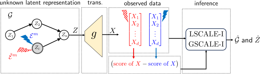
Figure 1: An overview of LSCALE-I and GSCALE-I algorithms. For each latent variable $Z_{i}$, there are two interventional mechanisms, denoted by red and blue. For each pair of environments, the score functions of observed variables are fed into GSCALE-I algorithm. Then, GSCALE-I uses this input to compute latent score differences for a given encoder and returns the encoder that minimizes these latent score differences. This encoder is used to compute estimates $\hat{\mathcal{G}}$ and $\hat{Z}$.

Organization.

The rest of the paper is organized as follows. Section 2 provides an overview of the literature with the main focus on CRL from interventions. Section 3 provides the preliminaries for formulating the problem and specifies the notations and definitions used throughout the paper. Section 4 summarizes our main identifiability and achievability results for both linear and general transformations and interprets them in the context of the existing literature. In Section 5, we introduce our score-based framework and design the CRL algorithms. In Section 6, we provide the details of the score-based methodology, analyze its key steps, and establish constructive proofs of the results in Section 4. Overviews of the proofs are presented in the main body of the paper, and the rest of the proofs are relegated to the appendices. Finally, in Section 7, we empirically assess the performance of the proposed CRL algorithms for recovering the latent causal variables and the latent causal graph.

2 Related Work

Table 1: Parametric Settings. Comparison of the results to prior studies in parametric settings. Only the main results of the most closely related studies are listed and standard shared assumptions are omitted. Formal definitions of identifiability measures are provided in Section 3.

Work	Transform	Latent	Int. Data	Identifiability
		Model	(one env. per node)	result
Squires et al. (2023)	Linear	Lin. Gaussian	Hard	perfect
	Linear	Lin. Gaussian	Soft	up to ancestors
Ahuja et al. (2023a)	Polynomial	General	do	perfect
	Polynomial	Bounded RV	Soft	perfect
Buchholz et al. (2023)	General	Lin. Gaussian	Hard	perfect
	General	Lin. Gaussian	Soft	up to ancestors
Zhang et al. (2023)	Polynomial	Non-linear	Soft	up to ancestors
	Polynomial	Non-linear (polytree)	Soft	perfect
Jin and Syrgkanis (2023)	Linear	Non-linear	Soft	perfect DAG and
	Linear	Lin. non-Gaussian	Soft	mixing w. surrounding
Theorem 1	Linear	General	Hard	perfect
Theorem 2	Linear	General	Soft	up to ancestors
Theorem 3	Linear	Non-linear	Soft	perfect DAG and
				mixing w. surrounding

In this paper, we address identifiability and achievability in CRL given different interventional environments in which the interventions act on the latent space. We first provide an overview of the literature that investigates CRL from interventional data, with the main results of the most closely related work summarized in Tables 1 and 2. Then, we discuss the other relevant lines of work.

Interventional causal representation learning.

The majority of the rapidly growing literature on CRL from interventions focuses on parametric settings, i.e., a parametric form is assumed for the latent model, the transformation, or both of them. Among related studies, Ahuja et al. (2023a) consider polynomial transformations without restrictions on the latent causal model and show identifiability under deterministic $do$ interventions. They also prove identifiability under soft interventions with independent support assumptions on latent variables. Squires et al. (2023) consider a linear latent model with a linear mapping to observations and prove identifiability under hard interventions. They also show the impossibility of perfect identifiability under soft interventions and prove identifiability up to ancestors. Buchholz et al. (2023) focus on linear Gaussian latent models and extend the results of Squires et al. (2023) to prove identifiability for general transformations. Zhang et al. (2023) consider polynomial transformations under nonlinearity assumptions on latent models and prove identifiability up to ancestors under soft interventions. If the latent graph is restricted to polytrees, they further prove perfect identifiability. Ahuja et al. (2023b) focus on identifying the non-intervened variables from the intervened variables by using single-node and multi-node soft interventions. They also consider a new setting in which the latent DAG can change across data points and rely on support invariance of non-intervened variables to identify them from the rest. Bing et al. (2023) consider a non-linear latent model under linear transformation and use multi-target $do$ interventions to prove identifiability under certain sparsity assumptions. Jin and Syrgkanis (2023) consider a linear transform and sufficiently non-linear latent models under a linear transform and prove identifiability up to surrounding parents using soft interventions . They also establish sufficient conditions for multi-target soft interventions to ensure identifiability. Saengkyongam et al. (2023) take a different approach and consider the task of intervention extrapolation. In their formulation, interventions are upon exogenous action variables (e.g., instrumental variables) which affect the latent variables linearly.

On the fully nonparametric setting, von Kügelgen et al. (2023) provide the most closely related identifiability results to ours. Specifically, they show that two coupled hard interventions per node suffice for identifiability under faithfulness assumption on latent causal models. Our results have two major differences: 1) We address achievability via a provably correct algorithm whereas von Kügelgen et al. (2023) focus mainly on identifiability (e.g., no algorithm for recovery of the latent variables), 2) we dispense with the restrictive assumptions on identifiability results, namely, we do not require to know which two environments share the same intervention target (hence, uncoupled interventions), and do not require faithfulness on the latent models. Among the other studies on the nonparametric setting, Jin and Syrgkanis (2023) provide analogous results to (von Kügelgen et al., 2023) by considering two coupled soft interventions and identifying latent variables up to mixing with surrounding variables. Jiang and Aragam (2023) consider identifying the latent DAG without recovering latent variables, where it is shown that a restricted class of DAGs can be recovered.

Weakly supervised causal representation learning.

A commonly used weak supervision signal for proving identifiability is assuming access to multi-view data, i.e., counterfactual pairs of observations arising from pre- and post-intervention observations (Locatello et al., 2020; von Kügelgen et al., 2021; Brehmer et al., 2022; Ahuja et al., 2022b). Yao et al. (2023) generalize the multi-view approach via a unified framework which also allows partial observability with non-linear transforms. Another approach is using temporal sequences to identify latent causal representations (Lachapelle et al., 2022; Yao et al., 2022; Lippe et al., 2023). Finally, some studies use stronger supervision signals such as the annotations of the ground truth causal variables or known causal graph (Shen et al., 2022; Liang et al., 2023). Among these, Liang et al. (2023) assume that the latent DAG is already known and recover the latent variables under hard interventions.

Table 2: General (Non-parametric) Settings. Comparison of the results to prior studies in the general setting. Formal definitions of identifiability measures are provided in Section 3. The shared assumptions (interventional discrepancy) and additional assumptions (faithfulness) are discussed in Section 4.

Work	Transform and	Obs.	Int. Data	Faithfulness	Identifiability	Provable
	Latent Model	Data	(env. per node)		result	algorithm
von Kügelgen et al. (2023)	General	No	2 coupled hard	Yes	perfect	✘
Jin and Syrgkanis (2023)	General	No	2 coupled soft	No	perfect DAG and	✘
					mixing w. surrounding
Theorem 4	General	Yes	2 uncoupled hard	No	perfect	✔
Theorem 5	General	Yes	2 coupled hard	No	perfect	✔
Theorem 6	General	No	2 coupled hard	Yes	perfect	✔

Identifiable representation learning.

As a special case of CRL, where the latent variables are independent, there is extensive literature on identifying latent representations. Some representative approaches include leveraging the knowledge of the mechanisms that govern the evolution of the system (Ahuja et al., 2022a) and using weak supervision with auxiliary information (Shu et al., 2020). Non-linear independent component analysis (ICA) also uses side information, in the form of structured time series to exploit temporal information (Hyvärinen and Morioka, 2017; Hälvä and Hyvärinen, 2020) or knowledge of auxiliary variables that renders latent variables conditionally independent (Khemakhem et al., 2020a, b; Hyvärinen et al., 2019). Morioka and Hyvärinen (2023) impose additional constraints on observational mixing and causal model to prove identifiability. Kivva et al. (2022) studies the identifiability of deep generative models without auxiliary information.

Score functions for causal discovery within observed variables.

Score matching has recently gained attraction in the causal discovery of observed variables. Rolland et al. (2022) use score matching to recover non-linear additive Gaussian noise models. The proposed method finds the topological order of causal variables but requires additional pruning to recover the full graph. Montagna et al. (2023b) focus on the same setting, recover the full graph from Jacobian scores, and dispense with the computationally expensive pruning stage. Montagna et al. (2023a) empirically demonstrate the robustness of score-matching-based approaches against the assumption violations in causal discovery. Also, Zhu et al. (2023) establish bounds on the error rate of score matching-based causal discovery methods. All of these studies are limited to observed causal variables, whereas in our case, we have a causal model in the latent space.

3 Preliminaries and Definitions

Notations.

For a vector $a\in{\mathbb{R}}^{m}$, the $i$-the entry is denoted by $a_{i}$. Matrices are denoted by bold upper-case letters, e.g., $\mathbf{A}$, where $\mathbf{A}_{i}$ denotes the $i$-th row of $\mathbf{A}$ and $\mathbf{A}_{i,j}$ denotes the entry at row $i$ and column $j$. For matrices $\mathbf{A}$ and $\mathbf{B}$ with the same shapes, $\mathbf{A}\preccurlyeq\mathbf{B}$ denotes component-wise inequality. We denote the indicator function by $\mathds{1}$, and for a matrix $\mathbf{A}\in{\mathbb{R}}^{m\times n}$, we use the convention that $\mathds{1}\{\mathbf{A}\}\in\{0,1\}^{m\times n}$, where the entries are specified by $[\mathds{1}\{\mathbf{A}\}]_{i,j}=\mathds{1}\{\mathbf{A}_{i,j}\neq 0\}$. For a positive integer $n\in{\mathbb{N}}$, we define $[n]\triangleq\{1,\dots,n\}$. The permutation matrix associated with any permutation $\pi$ of $[n]$ is denoted by $\mathbf{P}_{\pi}$, i.e., $[\pi_{1}\;\;\pi_{2}\;\dots\;\pi_{n}]^{\top}=\mathbf{P}_{\pi}\cdot[1\;\;2\;\dots\;n]^{\top}$. The $n$-dimensional identity matrix is denoted by $\mathbf{I}_{n\times n}$, and the Hadamard product is denoted by $\odot$. Given a function $f:{\mathbb{R}}^{r}\to{\mathbb{R}}^{s}$ that has first-order partial derivatives on ${\mathbb{R}}^{r}$, we denote the Jacobian of $f$ at $z\in{\mathbb{R}}^{s}$ by $J_{f}(z)$. We use $\operatorname{im}(f)$ to denote the image of $f$ and define rank of $f$ as the number of linearly independent vectors in its image and denote it by ${\mathcal{R}}(f)\triangleq\dim(\operatorname{im}(f))$. Accordingly, for a set of functions $\mathcal{F}\triangleq\{f_{i}:i\in[k]\ ,f_{i}:{\mathbb{R}}^{r}\to{\mathbb{R}}^{s}\}$ we define $\operatorname{im}(\mathcal{F})\triangleq\cup_{i=1}^{k}\operatorname{im}(f_{i})$, and denote the rank of $\mathcal{F}$ by $\mathcal{R}(\mathcal{F})\triangleq\dim(\operatorname{im}(\mathcal{F}))$.

3.1 Latent Causal Structure

Consider latent causal random variables $Z\triangleq[Z_{1},\dots,Z_{n}]^{\top}$. An unknown transformation $g:{\mathbb{R}}^{n}\to{\mathbb{R}}^{d}$ generates the observable random variables $X\triangleq[X_{1},\dots,X_{d}]^{\top}$ from the latent variables $Z$ according to:

$$X=g(Z)\ .$$ (3)

We assume that $d\geq n$, and transformation $g$ is continuously differentiable and a diffeomorphism onto its image (otherwise, identifiability is ill-posed). We denote the image of $g$ by $\mathcal{X}\triangleq\operatorname{im}(g)\subseteq{\mathbb{R}}^{d}$. The probability density functions (pdfs) of $Z$ and $X$ are denoted by $p$ and $p_{X}$, respectively. We assume that $p$ is absolutely continuous with respect to the $n$-dimensional Lebesgue measure. Subsequently, $p_{X}$, which is defined on the image manifold $\operatorname{im}(g)$, is absolutely continuous with respect to the $n$-dimensional Hausdorff measure rather than $d$-dimensional Lebesgue measure. The distribution of latent variables $Z$ factorizes with respect to a DAG that consists of $n$ nodes and is denoted by $\mathcal{G}$. Node $i\in[n]$ of $\mathcal{G}$ represents $Z_{i}$ and $p$ factorizes according to:

$$p(z)=\prod_{i=1}^{n}p_{i}(z_{i}\;|\;z_{{\rm{pa}}(i)})\ ,$$ (4)

where ${\rm{pa}}(i)$ denotes the set of parents of node $i$ and $p_{i}(z_{i}\;|\;z_{{\rm{pa}}(i)})$ is the conditional pdf of $z_{i}$ given the variables of its parents. We use ${\rm{ch}}(i)$, ${\rm{an}}(i)$, and ${\rm{de}}(i)$ to denote the children, ancestors, and descendants of node $i$, respectively. Accordingly, for each node $i\in[n]$ we also define

$$\overline{{\rm{pa}}}(i)\triangleq{\rm{pa}}(i)\cup\{i\},\;\;\overline{{\rm{ch}}}(i)\triangleq{\rm{ch}}(i)\cup\{i\},\;\;\overline{{\rm{an}}}(i)\triangleq{\rm{an}}(i)\cup\{i\},\;\mbox{and}\;\overline{{\rm{de}}}(i)\triangleq{\rm{de}}(i)\cup\{i\}\ .$$ (5)

We denote the transitive closure and transitive reduction of $\mathcal{G}$ by $\mathcal{G}_{\rm tc}$ and $\mathcal{G}_{\rm tr}$, respectively. The parental relationships in these graphs are denoted by ${\rm{pa}}_{\rm tc}$ and ${\rm{pa}}_{\rm tr}$, and other graphical relationships are denoted similarly. Based on the modularity property, a change in the causal mechanism of node $i$ does not affect those of the other nodes. We also assume that all conditional pdfs $\{p_{i}(z_{i}\mid z_{{\rm{pa}}(i)}):i\in[n]\}$ are continuously differentiable with respect to all $z$ variables and $p(z)\neq 0$ for all $z\in{\mathbb{R}}^{n}$. We consider the general structural causal models (SCMs) based on which for each $i\in[n]$,

$$Z_{i}=f_{i}(Z_{{\rm{pa}}(i)},N_{i})\ ,$$ (6)

where $\{f_{i}:i\in[n]\}$ are general functions that capture the dependence of node $i$ on its parents and $\{N_{i}:i\in[n]\}$ account for the exogenous noise terms that we assume to have pdfs with full support. We specialize some of the results to additive noise SCMs, in which (6) becomes

$$Z_{i}=f_{i}(Z_{{\rm{pa}}(i)})+N_{i}\ .$$ (7)

Next, we provide a number of definitions that we will use frequently throughout the paper for formalizing the framework and analyzing it.

Definition 1 (Valid Causal Order)

We refer to a permutation $(\pi_{1},\dots,\pi_{n})$ of $[n]$ as a valid causal order if $\pi_{i}\in{\rm{pa}}(\pi_{j})$ indicates that $i<j$.

In this paper, without loss of generality, we assume that $(1,\dots,n)$ is a valid causal order. We also define a graphical notion that will be useful for presenting our results and analysis on CRL under a linear transformation.

Definition 2 (Surrounded Node)

Node $i\in[n]$ in DAG $\mathcal{G}$ is said to be surrounded if there exists another node $j\in[n]$ such that $\overline{{\rm{ch}}}(i)\subseteq{\rm{ch}}(j)$. We denote the set of nodes that surround $i\in[n]$ by $\operatorname{sur}(i)$, and the set of all nodes that are surrounded by $\mathcal{S}$, i.e.,

$$\operatorname{sur}(i) \triangleq\{j\in[n]\,:\,j\neq i\;\;,\;\;\overline{{\rm{ch}}}(i)\subseteq{\rm{ch}}(j)\}\ ,\quad\mbox{and}\quad\mathcal{S}\triangleq\{i\in[n]\,:\;\operatorname{sur}(i)\neq\emptyset\}\ .$$ (8)

Figure 2: Sample latent DAGs $\mathcal{G}$. (Left) The valid causal orders are $(1,2,3,4)$ and $(1,3,2,4)$, and only surrounded node is $4$ with $\operatorname{sur}(4)=\{2,3\}$. (Right) The only valid causal order is $(1,2,3)$, and the surrounded nodes are $\mathcal{S}=\{2,3\}$ with $\operatorname{sur}(2)=\{1\},\operatorname{sur}(3)=\{1,2\}$.

3.2 Score Functions

The score function associated with a pdf is defined as the gradient of its logarithm. The score function associated with $p$ is denoted by

$$s(z)\triangleq\nabla_{z}\log p(z)\ .$$ (9)

Noting the connection $X=g(Z)$, the density of $X$ under $\mathcal{E}^{0}$, denoted by $p_{X}$, is supported on an $n$-dimensional manifold $\mathcal{X}$ embedded in ${\mathbb{R}}^{d}$. Hence, specifying the score function of $X$ requires notions from differential geometry. For this purpose, we denote the tangent space of manifold $\mathcal{X}$ at point $x\in\mathcal{X}$ by $T_{x}\mathcal{X}$. Tangent vectors $v\in T_{x}\mathcal{X}$ are equivalence classes of continuously differentiable curves $\gamma\colon(-1,1)\to\mathcal{X}\subseteq{\mathbb{R}}^{d}$ with $\gamma(0)=x$ and $\gamma^{\prime}(0)=v$. Furthermore, given a function $f\colon\mathcal{X}\to{\mathbb{R}}$, denote its directional derivative at point $x\in\mathcal{X}$ along a tangent vector $v\in T_{x}\mathcal{X}$ by $D_{v}f(x)$, which is defined as

$$D_{v}f(x)\triangleq\left.\frac{\differential}{\differential t}(f\circ\gamma)(t)\right|_{t=0}\ ,$$ (10)

for any curve $\gamma$ in equivalence class $v$. The differential of $f$ at point $x\in\mathcal{X}$, denoted by $\differential f_{x}$, is the linear operator mapping tangent vector $v\in T_{x}\mathcal{X}$ to $D_{v}f(x)$ (Simon, 2014, p. 57), i.e.,

$$\differential f_{x}\colon T_{x}\mathcal{X}\ni v\mapsto D_{v}f(x)\in{\mathbb{R}}\ .$$ (11)

Let $\mathbf{B}\in{\mathbb{R}}^{d\times n}$ be a matrix for which the columns of $\mathbf{B}$ form an orthonormal basis for $T_{x}\mathcal{X}$. Denote the directional derivative of $f$ along the $i$-th column of $\mathbf{B}$ by $D_{i}f$ for all $i\in[n]$. Then, the differential operator can be expressed by the vector

$$Df(x)\triangleq\mathbf{B}\cdot\big{[}D_{1}f(x)\,\ldots\,D_{n}f(x)\big{]}^{\top}\in{\mathbb{R}}^{d}\ ,$$ (12)

such that

$$\differential f_{x}(v)=v^{\top}\cdot Df(x)\ ,\qquad\forall x\in\mathcal{X}\ ,\quad\forall v\in T_{x}\mathcal{X}\ .$$ (13)

Note that the differential operator $\differential f$ is a generalization of the gradient. Hence, we can generalize the definition of the score function using the differential operator by setting $f$ to the logarithm of pdf. Therefore, the score function of $X$ under $\mathcal{E}^{0}$ is specified as follows:

$$s_{X}(x)\triangleq D\log p_{X}(x)\ ,\qquad\forall x\in\mathcal{X}\ .$$ (14)

3.3 Intervention Mechanisms

We consider two types of interventions. A soft intervention on node $i$ (also referred to as imperfect intervention in literature), changes the conditional distribution $p_{i}(z_{i}\;|\;z_{{\rm{pa}}(i)})$ to a distinct conditional distribution, which we denote by $q_{i}(z_{i}\;|\;z_{{\rm{pa}}(i)})$. A soft intervention does not necessarily remove the functional dependence of an intervened node on its parents and rather alters it to a different mechanism. A stochastic hard intervention on node $i$ (also referred to as perfect intervention) is stricter than a soft intervention and removes the edges incident on $i$. A hard intervention on node changes $p_{i}(z_{i}\;|\;z_{{\rm{pa}}(i)})$ to $q_{i}(z_{i})$ that emphasizes the lack of dependence of $z_{i}$ on $z_{{\rm{pa}}(i)}$. Finally, we note that in some settings, we assume two hard interventions per node, in which case the two hard interventional mechanisms for node $i$ are denoted by two distinct pdfs $q_{i}(z_{i})$ and $\tilde{q}_{i}(z_{i})$.

Interventional environments.

We consider atomic interventional environments in which each environment one node is intervened in, as it is customary to the closely related CRL literature (Squires et al., 2023; Ahuja et al., 2023a; Buchholz et al., 2023). In some settings (linear transformation), we will have one interventional environment per node and denote the interventional environments by $\mathcal{E}\triangleq\{\mathcal{E}^{1},\dots,\mathcal{E}^{n}\}$, where we call $\mathcal{E}$ the atomic environment set. We denote the node intervened in environment $\mathcal{E}^{m}$ by $I^{m}\in[n]$. For other settings (general transformation), we will have two interventional environments per node and denote the second atomic environment set by $\tilde{\mathcal{E}}=\{\tilde{\mathcal{E}}^{1},\dots,\tilde{\mathcal{E}}^{n}\}$. Similarly, we denote the intervened node in $\tilde{\mathcal{E}}^{m}$ by $\tilde{I}^{m}$ for each $m\in[n]$. We assume that node-environment pairs are unspecified, i.e., the ordered intervention sets $\mathcal{I}\triangleq(I^{1},\dots,I^{n})$ and $\tilde{\mathcal{I}}\triangleq(\tilde{I}^{1},\dots,\tilde{I}^{n})$ are two unknown permutations of $[n]$. We also adopt the convention that $\mathcal{E}^{0}$ is the observational environment and $I^{0}\triangleq\emptyset$. Next, we define the notion of coupling between the environment sets $\mathcal{E}$ and $\tilde{\mathcal{E}}$.

Definition 3 (Coupled/Uncoupled Environments)

The two environment sets $\mathcal{E}$ and $\tilde{\mathcal{E}}$ are said to be coupled if for the unknown permutations $\mathcal{I}$ and $\tilde{\mathcal{I}}$ we know that $\mathcal{I}=\tilde{\mathcal{I}}$, i.e., the same node is intervened in environments $\mathcal{E}^{i}$ and $\tilde{\mathcal{E}}^{i}$. The two environment sets are said to be uncoupled if $\tilde{\mathcal{I}}$ is an unknown permutation of $\mathcal{I}$.

Next, we define $p^{m}$ as the pdf of $Z$ in environment $\mathcal{E}^{m}$. Hence, under soft and hard intervention for each $m\in[n]$, $p^{m}$ can be factorized as follows.

$$\mbox{soft intervention in }\mathcal{E}^{m}: \quad p^{m}(z)=q_{\ell}(z_{\ell}\;|\;z_{{\rm{pa}}(\ell)})\prod_{i\neq\ell}p_{i}(z_{i}\;|\;z_{{\rm{pa}}(i)})\ , \quad\mbox{where}\quad\ell=I^{m}\ ,$$ (15)

$$\mbox{hard intervention in }\mathcal{E}^{m}: \quad p^{m}(z)=q_{\ell}(z_{\ell})\prod_{i\neq\ell}p_{i}(z_{i}\;|\;z_{{\rm{pa}}(i)})\ , \quad\mbox{where}\quad\ell=I^{m}\ .$$ (16)

Similarly, we define $\tilde{p}^{m}$ as the pdf of $Z$ in $\tilde{\mathcal{E}}^{m}$, which can be factorized similarly to (16) with $\tilde{q}_{\ell}$ replaced with $q_{\ell}$. Hence, the score functions associated with $p^{m}$ and $\tilde{p}^{m}$ are specified as follows.

$$s^{m}(z)\triangleq\nabla_{z}\log p^{m}(z)\ ,\quad\mbox{and}\quad\tilde{s}^{m}(z)\triangleq\nabla_{z}\log\tilde{p}^{m}(z)\ .$$ (17)

We denote the score functions of the observed variables $X$ under $\mathcal{E}^{m}$ and $\tilde{\mathcal{E}}^{m}$ by $s^{m}_{X}$ and $\tilde{s}^{m}_{X}$, respectively. Note that the score functions change across different environments, which is induced by the changes in the distribution of $Z$. We use $Z^{m}$ and $X^{m}$ to denote the latent variables $Z$ and observed variables $X$ in environment $\mathcal{E}^{m}$, respectively. In Section 6.1, we investigate score discrepancies between $s$ and $s^{m}$ (or $\tilde{s}^{m}$) and characterize the relationship between the scores in the observational and interventional environments.

3.4 Identifiability and Achievability Objectives

The objective of CRL is to use observations $X$ generated by the observational and interventional environments and estimate the true latent variables $Z$ and causal relations among them captured by $\mathcal{G}$. The first objective is identifiability, which pertains to determining algorithm-agnostic sufficient conditions under which $Z$ and $\mathcal{G}$ can be recovered uniquely up to a permutation and element-wise transform which is the strongest form of recovery in CRL from interventions as shown in (von Kügelgen et al., 2023). The second objective is achievability, which refers to designing algorithms that are amenable to practical implementation and generate provably correct estimates for $Z$ and $\mathcal{G}$, foreseen by the identifiability guarantees. In this subsection, we provide the definitions needed for formalizing identifiability and achievability objectives.

We denote a generic estimator of $Z$ given $X$ by $\hat{Z}(X):{\mathbb{R}}^{d}\to{\mathbb{R}}^{n}$. We also consider a generic estimate of $\mathcal{G}$ denoted by $\hat{\mathcal{G}}$. In order to assess the fidelity of the estimates $\hat{Z}(X)$ and $\hat{\mathcal{G}}$ with respect to the ground truth $Z$ and $\mathcal{G}$, we provide the following identifiability measures. We start with specifying perfect identifiability, which is relevant for assessing the identifiability and achievability results under hard interventions.

Definition 4 (Perfect Identifiability)

To formalize perfect identifiability in CRL we define:

1. Perfect DAG recovery: DAG recovery is said to be perfect if $\hat{\mathcal{G}}$ is isomorphic to $\mathcal{G}$.

2. Perfect latent recovery: Given the estimator $\hat{Z}(X)$, latent recovery is said to be perfect if $\hat{Z}(X)$ is an element-wise diffeomorphism of a permutation of $Z$, i.e., there exists a permutation $\pi$ of $[n]$ and a set of functions $\{\phi_{i}:i\in[n]\}$ such that $\phi_{i}:{\mathbb{R}}\to{\mathbb{R}}$ and we have

   $$\hat{Z}(X)=\mathbf{P}_{\pi}\cdot\phi(Z)\ ,\qquad\forall Z\in{\mathbb{R}}^{n}\ ,$$ (18)

   where $\phi(Z)\triangleq(\phi_{1}(Z_{1}),\dots,\phi_{n}(Z_{n})$.

3. Scaling consistency: The estimator $\hat{Z}(X)$ is said to maintain scaling consistency if there exists a permutation $\pi$ of $[n]$ and a constant diagonal matrix $\mathbf{C}_{\rm s}\in{\mathbb{R}}^{n\times n}$ such that

   $$\hat{Z}(X)=\mathbf{P}_{\pi}\cdot\mathbf{C}_{\rm s}\cdot Z\ ,\qquad\forall Z\in{\mathbb{R}}^{n}\ .$$ (19)

We note that scaling consistency is a special case of perfect latent recovery in which the diffeomorphism in the perfect latent recovery is restricted to an element-wise scaling. Next, we provide partial identifiability measures which will be useful to assess the identifiability and achievability results under soft interventions.

Definition 5 (Partial Identifiability)

To formalize partial identifiability in CRL we define:

1. Transitive closure recovery: DAG recovery is said to maintain transitive closure if $\hat{\mathcal{G}}$ and $\mathcal{G}$ have the same ancestral relationships, i.e., ${\hat{\mathcal{G}}_{\rm tr}}$ is isomorphic to $\mathcal{G}_{\rm tr}$.

2. Mixing consistency up to ancestors: The estimator $\hat{Z}(X)$ is said to maintain mixing consistency up to ancestors if there exists a permutation $\pi$ of $[n]$ and a constant matrix $\mathbf{C}_{\rm an}\in{\mathbb{R}}^{n\times n}$ such that

   $$\hat{Z}(X)=\mathbf{P}_{\pi}\cdot\mathbf{C}_{\rm an}\cdot Z\ ,\qquad\forall Z\in{\mathbb{R}}^{n}\ ,$$ (20)

   where $\mathbf{C}_{\rm an}$ has non-zero diagonal entries and for all $j\notin\overline{{\rm{an}}}(i)$, $\mathbf{C}_{\rm an}$ satisfies $[\mathbf{C}_{\rm an}]_{i,j}=0$.

3. Mixing consistency up to surrounding parents: The estimator $\hat{Z}(X)$ is said to maintain mixing consistency up to surrounding parents if there exists a permutation $\pi$ of $[n]$ and a constant matrix $\mathbf{C}_{\rm sur}\in{\mathbb{R}}^{n\times n}$ such that

   $$\hat{Z}(X)=\mathbf{P}_{\pi}\cdot\mathbf{C}_{\rm sur}\cdot Z\ ,\qquad\forall Z\in{\mathbb{R}}^{n}\ ,$$ (21)

   where $\mathbf{C}_{\rm sur}$ has non-zero diagonal entries and for all $i\neq j$ and $j\notin\operatorname{sur}(i)$, $\mathbf{C}_{\rm sur}$ satisfies $[\mathbf{C}_{\rm sur}]_{i,j}=0$.

3.5 Algorithm-related Definitions

For formalizing the achievability results and designing the associated algorithms, generating the estimates $\hat{Z}(X)$ and $\hat{\mathcal{G}}$ is facilitated by estimating the inverse of $g$ based on the observed data $X$. Specifically, an estimate of $g^{-1}$, where $g^{-1}$ denotes the inverse of $g$, facilitates recovering $Z$ via $Z=g^{-1}(X)$ . Throughout the rest of this paper, we refer to $g^{-1}$ as the true encoder. To formalize the procedures of estimating $g^{-1}$, we define $\mathcal{H}$ as the set of possible valid encoders, i.e., candidates for $g^{-1}$. A function $h\in\mathcal{H}$ can be such a candidate if it is invertible, that is, there exists an associated decoder $h^{-1}$ such that $(h^{-1}\circ h)(X)=X$. Hence, the set of valid encoders is specified by

$$\mathcal{H}\triangleq\{h:\mathcal{X}\to{\mathbb{R}}^{n}\;\colon\;\exists h^{-1}:{\mathbb{R}}^{n}\to{\mathbb{R}}^{d}\;\;\mbox{such that }\;\;(h^{-1}\circ h)(X)=X\ ,\;\;\forall X\in\mathcal{X}\}\ .$$ (22)

Next, corresponding to any pair of observation $X$ and valid encoder $h\in\mathcal{H}$, we define $\hat{Z}(X;h)$ as an auxiliary estimate of $Z$ generated by applying the valid encoder $h$ on $X$, i.e.,

$$\hat{Z}(X;h)\triangleq h(X)=(h\circ g)(Z)\ ,\qquad\forall\;h\in\mathcal{H}\ \;,\;X\in\mathcal{X}\ .$$ (23)

The estimate $\hat{Z}(X;h)$ inherits its randomness from $X$, and its statistical model is governed by that of $X$ and the choice of $h$. To emphasize the dependence on $h$, we denote the score functions associated with the pdfs of $\hat{Z}(X;h)$ under environments $\mathcal{E}^{0}$, $\mathcal{E}^{m}$, and $\tilde{\mathcal{E}}^{m}$, respectively, by

$$s_{\hat{Z}}(\cdot;h)\ ,\quad s_{\hat{Z}}^{m}(\cdot;h),\quad\mbox{and}\quad\tilde{s}_{\hat{Z}}^{m}(\cdot;h)\ .$$ (24)

We will be addressing both general and linear transformations $g$. In the linear transformation setting, the true linear transformation $g$ is denoted by matrix $\mathbf{G}\in{\mathbb{R}}^{d\times n}$. Accordingly, we denote a valid linear encoder by $\mathbf{H}\in{\mathbb{R}}^{n\times d}$. For a given valid encoder $\mathbf{H}$, the associated valid decoder is given by its Moore-Penrose inverse, i.e., $\mathbf{H}^{{\dagger}}\triangleq\mathbf{H}^{\top}\cdot(\mathbf{H}\cdot\mathbf{H}^{\top})^{-1}$.

4 Identifiability and Achievability Results

In this section, we present the main identifiability and achievability results under various settings. We provide constructive proofs for these results, which serve as the results for both identifiability and achievability aspects. The constructive proofs are based on the CRL algorithms, the specifics of which, their properties, and their optimality guarantees are presented in Section 5. The proofs of the results presented in this section are provided in Appendices B and C. Our results are categorized into two main settings based on the models of transformation from latent to observed variables (i.e., function $g$): (i) linear transformation, and (ii) general (nonparametric) transformation. The main difference between the assumptions made for both settings is the number of interventional environments per node. Specifically, we investigate CRL under linear transformation with one intervention per node and we address both soft and hard interventions. For CRL under a general transformation, we consider two hard interventions per node, and we discuss both coupled and uncoupled interventions. In parallel to our score-based framework initially presented in (Varıcı et al., 2023), there have been advances in identifiability results. We will also discuss the relevance and distinctions of our results vis-á-vis the results in the existing literature.

4.1 CRL under Linear Transformations

Under a linear transformation, the general transformation model in (3) becomes:

$$X=\mathbf{G}\cdot Z\ ,$$ (25)

where $\mathbf{G}\in{\mathbb{R}}^{d\times n}$ is an unknown full-rank matrix mapping the latent variables to the observed ones. We recall that the main purpose of using interventions for CRL is that interventions inject proper statistical variations into the observed data. Subsequently, our approach to CRL is built on tracing such statistical variations via tracking the variations of the score functions associated with the interventional data. We will use one intervention per node and the set of interventional environments is $\mathcal{E}=\{\mathcal{E}^{1},\dots,\mathcal{E}^{n}\}$. We will show that the key step to recovering the true latent representations is identifying the valid encoders that render minimal variations in the scores. To ensure that the effect of an intervention on a parent of the target variable is different from its effect on the target variable itself, we adopt the following assumption for the case of linear transformations. This assumption holds for a wide range of models and is discussed in more detail in Section 4.3.

Assumption 1

For any environment $\mathcal{E}^{m}\in\mathcal{E}$, and for all $k\in{\rm{pa}}(I^{m})$, we have

$$\mathcal{R}\left(\begin{bmatrix}[s-s^{m}]_{k}\\[4.30554pt] [s-s^{m}]_{\ell}\end{bmatrix}\right)=2\,,\qquad\mbox{where}\quad\ell=I_{m}\ .$$ (26)

Based on this assumption, our first result for the linear transformation setting establishes that scaling consistency and perfect DAG recovery is possible by using one hard intervention per node. Furthermore, the score-based algorithms guarantee achieving these perfect recovery objectives.

Theorem 1 (Linear – One Hard Intervention)

Under Assumption 1 for linear transformations, using observational data and interventional data from one hard intervention per node suffice to

1. Identifiability: perfectly recover the latent DAG $\mathcal{G}$;

2. Identifiability: ensure the scaling consistency of the latent variables;

3. Achievability: achieve the above two guarantees (via Algorithm 1).

Proof: See Appendix B.7.

We note that the existing literature on CRL with linear transformations and one stochastic hard intervention restricts the latent causal model to linear Gaussian models (Squires et al., 2023; Buchholz et al., 2023). In contrast, Theorem 1 does not impose any restriction on the latent causal model and shows that one stochastic hard intervention per node is sufficient for the identifiability of general latent causal models.

Next, we extend the results to soft interventions. The major consequence of applying hard versus soft interventions is that the variations in the latent distributions caused by hard interventions are, in general, stronger than those caused by soft interventions. The reason is that the intervention target is not necessarily isolated from its parents under a soft intervention. Consequently, the identifiability guarantees for soft interventions are expected to be weaker. In the next theorem, we present partial identifiability results, defined in Definition 5, for soft interventions under the general latent causal models.

Theorem 2 (Linear – One Soft Intervention)

Under Assumption 1 for linear transformations, using observational data and interventional data from one soft intervention per node suffice to

1. Identifiability: recover the transitive closure of the latent DAG $\mathcal{G}$;

2. Identifiability: ensure the mixing consistency of the latent variables up to ancestors;

3. Achievability: achieve the above two guarantees (via Algorithm 1).

Proof: See Appendix B.7.

Similar to the restrictions in the existing results for hard interventions, the transitive closure recovery results in the existing literature require the latent causal model to be either linear Gaussian (Squires et al., 2023; Buchholz et al., 2023) or satisfy non-linearity conditions (Zhang et al., 2023). In contrast, Theorem 2 achieves transitive closure recovery and mixing consistency up to ancestors without imposing any restrictions on the latent causal model.

For linear transformations, finally, we investigate the conditions under which soft interventions are guaranteed to achieve identifiability results stronger than transitive closure and mixing up to ancestors. In particular, we specify one condition on the rank of the score function differences $(s-s^{m})$, formalized next.

Assumption 2 (Full-rank Score Difference)

For all interventional environments $\mathcal{E}^{m}\in\mathcal{E}$ we have

$$\mathcal{R}(s-s^{m})=|\overline{{\rm{pa}}}(I^{m})|\ .$$ (27)

For insight into this assumption, it can be readily verified that for linear Gaussian latent models $\mathcal{R}(s-s^{m})\leq 2$ and on the other hand, for sufficiently non-linear causal models, $\mathcal{R}(s-s^{m})$ is $\overline{{\rm{pa}}}(I^{m})$. This assumption is stronger than Assumption 1 since it implies that the effects of an intervention on all parents of the target variable are different. We will provide more discussions on this assumption in Section 4.3. The next theorem tightens the identifiability and achievability guarantees of Theorem 2 under Assumption 2.

Theorem 3 (Linear – One Soft Intervention)

Under Assumption 2 for linear transformations, using observational data and interventional data from one soft intervention per node suffice to

1. Identifiability: perfectly recover the latent DAG $\mathcal{G}$;

2. Identifiability: ensure the mixing consistency of the latent variables up to surrounding parents;

3. Achievability: achieve the above two guarantees (via Algorithm 1).

Proof: See Appendix B.7.

Theorem 3 has two important implications. First, the latent DAG can be identified using only soft interventions under mild non-linearity assumptions on the latent causal model. To our knowledge, this is the first result in the literature for fully recovering latent DAG with soft interventions without restricting the graphical structure, e.g., Zhang et al. (2023) require linear faithfulness assumption to achieve similar results, which is only shown to hold for non-linear latent models with polytree structure. Secondly, the estimated latent variables reveal the true conditional independence relationships since they satisfy the Markov property with respect to the estimated latent DAG, which is isomorphic to the true DAG. Recalling that the motivation of CRL is learning useful representations that preserve causal relationships, our result shows that it can be achieved without perfect identifiability for a large class of models.

4.2 CRL under General Transformations

In this setting, we consider general transformations without any parametric assumption for transformation $g$. We use two interventional environments per node, which are expected to provide more information compared to one intervention per node setting for linear transformations. The sets of interventions are $\mathcal{E}=\{\mathcal{E}^{1},\dots,\mathcal{E}^{n}\}$ and $\tilde{\mathcal{E}}=\{\tilde{\mathcal{E}}^{1},\dots,\tilde{\mathcal{E}}^{n}\}$. For being informative, we assume that the two intervention mechanisms per node are sufficiently distinct. This is formalized by defining interventional discrepancy (Liang et al., 2023) among the causal mechanisms of a latent variable.

Definition 6 (Interventional Discrepancy)

Two intervention mechanisms with pdfs $p,q:{\mathbb{R}}\to{\mathbb{R}}$ are said to satisfy interventional discrepancy if

$$\frac{\partial}{\partial u}\frac{p(u)}{q(u)}\neq 0\ ,\quad{\forall u\in{\mathbb{R}}\setminus\mathcal{T}}\ ,$$ (28)

where $\mathcal{T}$ is a null set (i.e., has a zero Lebesgue measure).

This assumption ensures that the two distributions are sufficiently different. As shown by Liang et al. (2023), even when the latent graph $\mathcal{G}$ is known, for identifiability via one intervention per node, it is necessary to have interventional discrepancy between observational distribution $p_{i}$ and interventional distribution $q_{i}$, for all $z_{{\rm{pa}}(i)}\in{\mathbb{R}}^{|{\rm{pa}}(i)|}$.

Our main result for general transformations establishes that perfect identifiability is possible given two atomic environment sets, even when the environments corresponding to the same node are not specified in pairs. That is, not only is it unknown what node is intervened in an environment, additionally the learner also does not know which two environments intervene on the same node.

Theorem 4 (General – Uncoupled Environments)

Using observational data and interventional data from two uncoupled hard environments for which each pair in $\{p_{i},q_{i},\tilde{q}_{i}\}$ satisfies interventional discrepancy, suffices to

1. Identifiability: perfectly recover the latent DAG $\mathcal{G}$;

2. Identifiability: perfectly recover the latent variables;

3. Achievability: achieve the above two guarantees (via Algorithm 5).

Proof: See Appendix C.5.

Theorem 4 shows that using observational data enables us to resolve any mismatch between the uncoupled environment sets and shows identifiability in the setting of uncoupled environments. This generalizes the identifiability result of von Kügelgen et al. (2023), which requires coupled environments. Importantly, Theorem 4 does not require faithfulness whereas the study in (von Kügelgen et al., 2023) requires that the estimated latent distribution is faithful to the associated candidate graph for all $h\in\mathcal{H}$. Even though a faithfulness assumption does not compromise the identifiability result, it is a strong requirement to verify and poses challenges to devising recovery algorithms. In contrast, we only require observational data, which is generally accessible in practice. Based on this, we design a score-based algorithm, which is presented and discussed in Section 5. Next, if the environments are coupled, we prove perfect latent recovery under weaker assumptions on the interventional discrepancy.

Theorem 5 (General – Coupled Environments)

Using observational data and interventional data from two uncoupled hard environments for which the pair $(p_{i},q_{i})$ satisfies interventional discrepancy for all $i\in[n]$, suffices to

1. Identifiability: perfectly recover the latent DAG $\mathcal{G}$;

2. Identifiability: perfectly recover the latent variables;

3. Achievability: achieve the above two guarantees (via Algorithm 5).

Proof: See Appendix C.1.

In the proof of Theorem 5, we show that the advantage of environment coupling is that it renders interventional data sufficient for perfect latent recovery, and the observational data is only used for recovering the graph. We further tighten this result by showing that for DAG recovery, the observational data becomes unnecessary when we have additive noise models and a weak faithfulness condition holds.

Theorem 6 (No Observational Data)

Using interventional data from two coupled hard environments for which the pair $(q_{i},\tilde{q}_{i})$ satisfies interventional discrepancy for all $i\in[n]$, suffices to

1. Identifiability: perfectly recover the latent DAG $\mathcal{G}$ if the latent causal model has additive noise, $p(Z)$ is twice differentiable, and it satisfies the adjacency-faithfulness ;

2. Identifiability: perfectly recover the latent variables

3. Achievability: achieve the above two guarantees.

Proof: See Appendix C.2.

Finally, we remark that the main results in this subsection (i.e., Theorem 4 and 5) hold for any latent causal model. The additive noise model assumption is required only for the DAG recovery part of Theorem 6.

4.3 Discussion on Assumptions 1 and 2

In this subsection, we elaborate on Assumptions 1 and  2, which are relevant to Theorems 2 and 3, respectively. Assumption 1 essentially states that score changes in the coordinates of the intervened node and a parent of the intervened node are linearly independent. This property holds for (but is not limited to) the widely adopted additive noise models specified in (7) when we apply hard interventions. This property is formalized in the next lemma.

Lemma 1

Assumption 1 is satisfied for additive noise models under hard interventions.

Proof: See Appendix D.1.

When soft interventions are applied, we note that even partial identifiability is shown to be impossible without making assumptions about the effect of the interventions. Specifically, for linear latent causal models, Buchholz et al. (2023) prove impossibility results for pure shift interventions and Squires et al. (2023) show that a genericity condition is necessary for identifying the transitive closure of the latent DAG. Therefore, Assumption 1 can be interpreted as the counterpart of the commonly adopted assumptions in the literature on soft interventions adapted to the setting of general latent causal models.

Given the known result that perfect identifiability is impossible for linear Gaussian models given soft interventions, the purpose of Assumption 2 is to get more insight into the extent of identifiability guarantees under soft interventions. Intuitively, the mentioned impossibility results for linear Gaussian models are due to the rank deficiency of score differences for linear models – specifically, we know that $\mathcal{R}(s-s^{m})\leq 2$ for linear Gaussian models. In contrast, for sufficiently non-linear causal models, $\mathcal{R}(s-s^{m})$ can be as high as $\overline{{\rm{pa}}}(I^{m})$. Assumption 2 ensures that this upper bound is satisfied with equality for all nodes. This condition holds for the class of sufficiently non-linear models, such as quadratic causal models. In particular, we show that this condition holds for the two-layer neural networks (NNs) as a function class that can effectively approximate any continuous function. This result is formalized in the next lemma.

Lemma 2

Consider the additive model in (7) where $f_{i}$ is a two-layer NN with sigmoid activation function, and weight matrices $\mathbf{W}^{i}$ and $\bar{\mathbf{W}}^{i}$ for observational and interventional mechanisms, respectively. If $\max\{\rank(\mathbf{W}^{i})\,,\,\rank(\bar{\mathbf{W}}^{i})\}=|{\rm{pa}}(i)|$ for all $i\in[n]$, then Assumption 2 holds.

We discuss the non-linearity and the proof of Lemma 2 in Appendix D.2.

5 Score-based Algorithms for CRL

This section serves a two-fold purpose. First, it provides the constructive proof and the steps involved in it for establishing the identifiability results for (i) linear transformations (Theorems 1 and 2) and (ii) general transformations (Theorems 4 and 5). Secondly, it provides achievability via designing algorithms that have provable guarantees for the perfect recovery of the latent variables and latent DAG for (i) linear transformations, in which perfect recovery of latent variables improved to scaling consistency, and (ii) any general class of functions (linear and non-linear). These algorithms are referred to as Linear Score-based Causal Latent Estimation via Interventions (LSCALE-I) for the linear setting, and Generalized Score-based Causal Latent Estimation via Interventions (GSCALE-I) for the general setting. Various properties of these algorithms and the attendant achievability guarantee analyses are presented in Section 6.

The key idea of the score-based framework is that tracing the changes in the score functions of the latent variables guides finding reliable estimates for the inverse of transformation $g$, which in turn facilitates estimating $Z$. However, the scores of the latent variables are not directly accessible. To circumvent this, we establish a connection between the score functions of the latent variables and those of the observed variables $X$, which are accessible. Based on this, we first compute the score functions of the accessible observed variables $X$, and then leverage the established connection to determine the needed score functions of the latent variables. Finally, we note that we are interested only in the changes in the score functions. Hence, we do not directly require the score functions themselves but rather need their differences. Lemma 4 in Section 6 establishes that the changes in the score functions of the latent variables can be traced from the changes in the score functions of the observed variables. Given any valid encoder $h$, based on (23), the estimated latent variable $\hat{Z}(X;h)$ and $X$ are related through $\hat{Z}(X;h)=h(X)$. We use this relationship to characterize the connection between the score differences as follows, which is formalized in Lemma 4 in Section 6.

$$\mbox{between }\mathcal{E}^{0}\mbox{ and }\mathcal{E}^{m} :\quad s_{\hat{Z}}(\hat{z};h)-s^{m}_{\hat{Z}}(\hat{z};h)=\big{[}J_{h^{-1}}(\hat{z})\big{]}^{\top}\cdot\big{[}s_{X}(x)-s^{m}_{X}(x)\big{]}\ ,$$ (29)

$$\mbox{between }\mathcal{E}^{0}\mbox{ and }\tilde{\mathcal{E}}^{m} :\quad s_{\hat{Z}}(\hat{z};h)-\tilde{s}^{m}_{\hat{Z}}(\hat{z};h)=\big{[}J_{h^{-1}}(\hat{z})\big{]}^{\top}\cdot\big{[}s_{X}(x)-\tilde{s}^{m}_{X}(x)\big{]}\ ,$$ (30)

$$\mbox{between }\mathcal{E}^{m}\mbox{ and }\tilde{\mathcal{E}}^{m} :\quad s^{m}_{\hat{Z}}(\hat{z};h)-\tilde{s}^{m}_{\hat{Z}}(\hat{z};h)=\big{[}J_{h^{-1}}(\hat{z})\big{]}^{\top}\cdot\big{[}s^{m}_{X}(x)-\tilde{s}^{m}_{X}(x)\big{]}\ .$$ (31)

Next, we provide the algorithms for linear and general transformation settings.

Algorithm 1 Linear Score-based Causal Latent Estimation via Interventions (LSCALE-I)

1:Input: Samples of $X$ from environment $\mathcal{E}^{0}$ and environment set $\mathcal{E}$

2:Step L1: Compute score differences: $(s_{X}-s_{X}^{m})$ for all $m\in[n]$

3:Step L2: Apply Algorithm 2: obtain a causal order $\pi$ and initial estimate for encoder $\mathbf{H}$

4:Step L3: Apply Algorithm 3: Minimize score variations to obtain the transitive reduction of the graph and update the encoder estimate

5:if the interventions are hard then

6:     Step L4: Apply Algorithm 4: Resolve the mixing with ancestors

7:end if

8:Return $\hat{\mathcal{G}}$ and $\hat{Z}$

5.1 LSCALE-I Algorithm for Linear Transformations

We provide the details of the algorithm Linear Score-based Causal Latent Estimation via Interventions (LSCALE-I). The algorithm is summarized in Algorithm 1 and the steps involved are described next.

Algorithm 2 Obtain Causal Order

1:Input: Samples of $X$ from environment $\mathcal{E}^{0}$ and environment set $\mathcal{E}$

2:Initialize $\mathbf{A}=\boldsymbol{0}_{n\times d}$ $\triangleright$ $\mathbf{A}$ holds for the estimate of $\big{(}\mathbf{H}^{{\dagger}}\big{)}^{\top}$

3:$\mathcal{V}_{n}=\{1,\dots,n\}$ $\triangleright$ remaining unordered set

4:for $t\in(n,\dots,1)$ do

5:     $\mathcal{F}_{t}=\operatorname{im}(\mathbf{G})\setminus\operatorname{span}(\mathbf{A}_{\pi_{t+1}}^{\top},\dots,\mathbf{A}_{\pi_{n}}^{\top})$ $\triangleright$ define the feasible set

6:     for $k\in\mathcal{V}_{t}$ do

$$c=\min_{a\;\in\;\mathcal{F}_{t}}\sum_{m\in\mathcal{V}_{t}\setminus\{k\}}{\mathbb{E}}\bigg{[}\Big{|}a^{\top}\cdot\big{[}s_{X}(X)-s_{X}^{m}(X)\big{]}\Big{|}\bigg{]}$$ (32)

7:         if $c=0$ then

8:              Denote a minimizer by $a^{*}$ and set $\mathbf{A}_{k}^{\top}=a^{*}$ $\triangleright$ the intermediate estimate

9:              $\pi_{t}=k$ $\triangleright$ $I^{k}$ has no descendants in $I^{\mathcal{V}_{t}}$

10:              $\mathcal{V}_{t-1}=\mathcal{V}_{t}\setminus\{\pi_{t}\}$ $\triangleright$ remove the identified node from unordered set

11:              break

12:         end if

13:     end for

14:end for

15:Return $\pi$ and $\mathbf{A}$

Algorithm 3 Minimize Score Variations

1:Input: Samples of $X$ from environment $\mathcal{E}^{0}$ and environment set $\mathcal{E}$, and $\{\pi,A\}$ generated by Algorithm 2

2:Initialize $\hat{\mathcal{G}}$ with empty graph over nodes $\{\pi_{1},\dots,\pi_{n}\}$

3:for $t\in(n-1,\dots,1)$ do

4:     $\mathcal{F}_{t}=\operatorname{im}(\mathbf{G})\setminus\operatorname{span}(\mathbf{A}_{\pi_{t+1}}^{\top},\dots,\mathbf{A}_{\pi_{n}}^{\top})$ $\triangleright$ update the feasible set

5:     for $j\in\{t+1,\dots,n\}$ do

6:         if Assumption 2 holds then $\triangleright$ set for determining whether $\pi_{t}\rightarrow\pi_{j}$

7:              $\mathcal{M}_{t,j}=\mathcal{V}_{j}\setminus\big{\{}{\hat{\rm{ch}}}(\pi_{t})\cup\{\pi_{t}\}\big{\}}$

8:         else

9:              $\mathcal{M}_{t,j}=\mathcal{V}_{j}\setminus\big{\{}{\hat{\rm{de}}}(\pi_{t})\cup\{\pi_{t}\}\big{\}}$

10:         end if

11:         

$$c=\min_{a\;\in\;\mathcal{F}_{t}}\sum_{m\in\mathcal{M}_{t,j}}{\mathbb{E}}\bigg{[}\Big{|}a^{\top}\cdot\big{[}s_{X}(X)-s_{X}^{m}(X)\big{]}\Big{|}\bigg{]}$$ (33)

12:         if $c=0$ then

13:              Denote a minimizer by $a^{*}$ and set $\mathbf{A}_{\pi_{t}}^{\top}=a^{*}$ $\triangleright$ update the estimate

14:         else

15:              Add $\pi_{t}\rightarrow\pi_{j}$ to $\hat{\mathcal{G}}$

16:         end if

17:     end for

18:end for

19:Encoder estimate: $\mathbf{H}^{*}=\big{(}\mathbf{A}^{\top}\big{)}^{{\dagger}}$

20:Return $\hat{\mathcal{G}}$ and $\mathbf{H}^{*}$

Inputs:

The inputs of LSCALE-I are the observed data from the observational environment, the data from one interventional environment per node, and $\operatorname{im}(\mathbf{G})$. We can estimate $\operatorname{im}(\mathbf{G})$ correctly from $n$ random samples of $X$ using singular value decomposition with probability $1$.

Step L1 - Score differences:

We start by computing score differences $(s_{X}-s_{X}^{m})$ for all $m\in[n]$.

Step L2 - Obtaining a causal order:

The initial observation is that the image of $(s_{X}-s_{X}^{m})$ for different values of $m$ are sufficiently different. Hence, an encoder cannot simultaneously make the estimated latent score differences equal to zero for all environments. However, this becomes possible when a leaf node is excluded. Subsequently, the key idea in this step is searching for the environment for which the latent score differences can be made zero for all the remaining environments. By following this routine, Algorithm 2 finds the youngest node among the remaining ones at each step and returns a permutation $\pi$ of the nodes. In Lemma 7, we show that the permutation $I^{\pi}\triangleq(I^{\pi_{1}},\dots,I^{\pi_{n}})$ is a valid causal order.

Step L3 - Identifying ancestors via minimizing score variations:

After obtaining a valid causal order for the intervened nodes in the environments, we perform Algorithm 3 to estimate children of a node in the latent DAG at each step and construct our encoder estimate $\mathbf{H}^{*}$. In Lemma 8, we show that the outputs of this step achieve identifiability up to ancestors, that is, $\hat{\mathcal{G}}_{\rm tr}$ is isomorphic to $\mathcal{G}_{\rm tr}$ under permutation $\pi$, and $\hat{Z}_{\pi_{i}}$ is a linear function of $\{Z_{j}:j\in\overline{{\rm{an}}}(i)\}$ for all $i\in[n]$.

Step L4 - Hard interventions to resolve mixing with ancestors:

We have this additional step in the case of hard interventions to further refine our estimates and achieve perfect identifiability. Specifically, we use the fact that the intervened latent variable becomes independent of its non-descendants. Algorithm 4 uses this critical property to construct an unmixing matrix $\mathbf{V}$ and refines our encoder estimate as $\mathbf{H}^{*}=\mathbf{V}\cdot\mathbf{H}^{*}$. For a perfect DAG recovery, we compute the latent score differences and construct the graph $\hat{\mathcal{G}}$ based on the following rule.

$$i\in\big{\{}\hat{{\rm{pa}}}(m)\cup\{m\}\big{\}}\iff{\mathbb{E}}\bigg{[}\Big{|}\big{[}s_{\hat{Z}}(\hat{Z};\mathbf{H}^{*})-s_{\hat{Z}}^{m}(\hat{Z};\mathbf{H}^{*})\big{]}_{i}\Big{|}\bigg{]}\neq 0\ ,$$ (34)

In Lemma 10, we show that $\hat{\mathcal{G}}$ is isomorphic to $\mathcal{G}$ and $\hat{Z}(X;\mathbf{H}^{*})$ satisfies scaling consistency.

Algorithm 4 Unmixing Procedure

1:Input: Samples of $X$ from environment $\mathcal{E}^{0}$ and environment set $\mathcal{E}$, $\pi$ from Algorithm 2 and $\mathbf{H}^{*}$ from Algorithm 3

2:Initialize $\mathbf{V}=\mathbf{I}_{n\times n}$

3:for $k\in(1,\dots,n)$ do

4:     Initialize $\mathbf{A}=\boldsymbol{0}_{(k-1)\times(k-1)}$

5:     $\hat{Z}^{\pi_{k}}=\mathbf{H}^{*}\cdot X^{\pi_{k}}$

6:     for $j\in\{1,\dots,k-1\}$ do

7:         $\tilde{Z}_{\pi_{j}}=\mathbf{V}_{\pi_{j}}\cdot\hat{Z}^{\pi_{k}}$

8:     end for

9:     for $j,\ell\in\{1,\dots,k-1\}$ do

10:         $\mathbf{A}_{j,\ell}=\operatorname{Cov}(\hat{Z}^{\pi_{k}}_{\pi_{j}},\tilde{Z}_{\pi_{\ell}})$

11:     end for

12:     $b=\operatorname{Cov}\big{(}\hat{Z}^{\pi_{k}}_{\pi_{k}},[\tilde{Z}_{\pi_{1}},\dots,\tilde{Z}_{\pi_{k-1}}]\big{)}$

13:     for $j\in\{1,\dots,k-1\}$ do

14:         $\mathbf{V}_{\pi_{k},\pi_{j}}=-[\mathbf{A}^{-1}\cdot b]_{j}$

15:     end for

16:end for

17:Update the encoder estimate: $\mathbf{H}^{*}=\mathbf{V}\cdot\mathbf{H}^{*}$

18:Latent DAG recovery: Construct $\hat{\mathcal{G}}$ according to (34).

19:return $\hat{\mathcal{G}}$ and $\mathbf{H}^{*}$

5.2 GSCALE-I Algorithm for General Transformations

In the LSCALE-I algorithm, we have exploited the transformation’s linearity and recovered the true encoder’s parameters sequentially using one intervention per node. For general transformations (parametric or non-parametric), however, we cannot use the same parametric approach and rely on the properties of linear transforms. To rectify these and design the general algorithm, we use more information in the form of two interventions per node. Specifically, we design the GSCALE-I algorithm, which directly minimizes the score differences across interventional environment pairs. We emphasize that the structure of this algorithm is different from the LSCALE-I algorithm, and feeding it with data from one intervention per node does not reduce it to LSCALE-I. Specifically, there are major differences in Step G2 and Step L3, as Step G2 of GSCALE-I directly minimizes the score differences for hard interventions, whereas Step L3 of LSCALE-I is designed to sequentially minimize the score differences for soft interventions which subsume hard interventions.

The core tool for identifiability via the GSCALE-I algorithm is that among all valid encoders $h\in\mathcal{H}$, the true encoder $g^{-1}$ results in the minimum number of variations between the score estimates $s^{m}_{\hat{Z}}(\hat{z};h)$ and $\tilde{s}^{m}_{\hat{Z}}(\hat{z};h)$ (see Lemma 11). To formalize these, corresponding to each valid encoder $h\in\mathcal{H}$, we define score change matrices $\mathbf{D}_{\rm t}(h)$, $\mathbf{D}(h)$, and $\tilde{\mathbf{D}}(h)$ as follows. For all $i,m\in[n]$:

$$[\mathbf{D}_{\rm t}(h)]_{i,m}\triangleq{\mathbb{E}}\Big{[}\,\Big{|}\big{[}s_{\hat{Z}}^{m}(\hat{Z};h)-\tilde{s}_{\hat{Z}}^{m}(\hat{Z};h)\big{]}_{i}\Big{|}\,\Big{]}\ ,$$ (35)

$$[\mathbf{D}(h)]_{i,m}\triangleq{\mathbb{E}}\Big{[}\,\Big{|}\big{[}s_{\hat{Z}}(\hat{Z};h)-s_{\hat{Z}}^{m}(\hat{Z};h)\big{]}_{i}\Big{|}\,\Big{]}\ ,$$ (36)

$$[\tilde{\mathbf{D}}(h)]_{i,m}\triangleq{\mathbb{E}}\Big{[}\,\Big{|}\big{[}s_{\hat{Z}}(\hat{Z};h)-\tilde{s}_{\hat{Z}}^{m}(\hat{Z};h)\big{]}_{i}\Big{|}\,\Big{]}\ ,$$ (37)

where expectations are under the measures of latent score functions induced by the probability measure of observational data. The entry $[\mathbf{D}_{\rm t}(h)]_{i,m}$ will be strictly positive only when there is a set of samples $X$ with a strictly positive measure that renders non-identical scores $s^{m}_{\hat{Z}}(\hat{z};h)$ and $\tilde{s}^{m}_{\hat{Z}}(\hat{z};h)$. Similar properties hold for the entries of $\mathbf{D}(h)$ and $\tilde{\mathbf{D}}(h)$ for the respective score functions. The GSCALE-I algorithm is summarized in Algorithm 5, and the steps involved are described next. We note that this algorithm serves the two purposes of providing a constructive proof of identifiability and provably correct achievability. We present the steps in the most general form to address both aspects and then we elaborate more on the practical considerations pertinent to achievability in Remark 1.

Algorithm 5 Generalized Score-based Causal Latent Estimation via Interventions (GSCALE-I)

1:Input: $\mathcal{H}$, samples of $X$ from environment $\mathcal{E}^{0}$ and environment sets $\mathcal{E}$ and $\tilde{\mathcal{E}}$, is_coupled.

2:Step G1: Compute score differences:$(s_{X}-s_{X}^{m}),(s_{X}-\tilde{s}_{X}^{m})$, and $(s_{X}^{m}-\tilde{s}_{X}^{m})$ for all $m\in[n]$.

3:Step G2: Identify the encoder by minimizing score variations:

4:if is_coupled then

5:     Solve $\mathcal{P}_{1}$ in (38), select a solution $h^{*}$.

6:else$\triangleright$ search for the correct coupling

7:     for all permutations $\pi$ of $[n]$ do

8:         Temporarily relabel $\tilde{\mathcal{E}}^{m}$ to $\tilde{\mathcal{E}}^{\pi_{m}}$ for all $m\in[n]$, and solve $\mathcal{P}_{2}$ in (39)

9:         If there is a solution, select a solution $h^{*}$ and break from the loop.

10:     end for

11:end if

12:Step G3: Latent estimates: $\hat{Z}=h^{*}(X)$.

13:Step G4: Latent DAG recovery: Construct latent DAG $\hat{\mathcal{G}}$ using (40).

14:return $\hat{Z}$ and $\hat{\mathcal{G}}$.

Inputs:

The inputs of GSCALE-I are the observed data from the observational and two interventional environments, whether environments are coupled/uncoupled, and a set of valid encoders $\mathcal{H}$.

Step G1 – Score differences:

We start by computing score differences $(s_{X}-s_{X}^{m}),(s_{X}-\tilde{s}_{X}^{m})$, and $(s_{X}^{m}-\tilde{s}_{X}^{m})$ for all $m\in[n]$.

Step G2 – Identifying the encoder:

The key property in this step is that the number of variations of the estimated latent score differences is always no less than the number of variations of the true latent score differences. We have two different approaches for coupled and uncoupled settings.

Step G2 (a) – Coupled environments:

We solve the following optimization problem

$$\mathcal{P}_{1}\triangleq\left\{\begin{aligned} \min_{h\in\mathcal{H}}\quad&\|\mathbf{D}_{\rm t}(h)\|_{0}\\ \mbox{s.t.}\quad&\mathbf{D}_{\rm t}(h)\;\;\mbox{is a diagonal matrix}\ .\end{aligned}\right.$$ (38)

Constraining $\mathbf{D}_{\rm t}(h)$ to be diagonal enforces that the final estimate $\hat{Z}$ and $Z$ will be related by permutation $\mathcal{I}$ (the intervention order). We select a solution of $\mathcal{P}_{1}$ in (38) as our encoder estimate and denote it by $h^{*}$.

Step G2 (b) – Uncoupled environments:

In this setting, additionally, we need to determine the correct coupling between the interventional environment sets $\mathcal{E}$ and $\tilde{\mathcal{E}}$. To this end, we iterate through permutations $\pi$ of $[n]$, and temporarily relabel $\tilde{\mathcal{E}}^{m}$ to $\tilde{\mathcal{E}}^{\pi_{m}}$ for all $m\in[n]$ within each iteration. Subsequently, we solve the following optimization problem:

$$\mathcal{P}_{2}\triangleq\left\{\begin{aligned} \min_{h\in\mathcal{H}}\quad&\|\mathbf{D}_{\rm t}(h)\|_{0}\\ \mbox{s.t.}\quad&\mathbf{D}_{\rm t}(h)\;\;\mbox{is a diagonal matrix}\\ &\mathds{1}\{\mathbf{D}(h)\}=\mathds{1}\{\tilde{\mathbf{D}}(h)\}\\ &\mathds{1}\{\mathbf{D}(h)\}\odot\mathds{1}\{\mathbf{D}^{\top}(h)\}=\mathbf{I}_{n\times n}\ .\end{aligned}\right.$$ (39)

The constraint $\mathds{1}\{\mathbf{D}(h)\}=\mathds{1}\{\tilde{\mathbf{D}}(h)\}$ ensures that a permutation of the correct encoder is a solution to $\mathcal{P}_{2}$ if the coupling is correct, and the last constraint ensures that $\mathbf{D}(h)$ does not contain 2-cycles. We will show that $\mathcal{P}_{2}$ is always feasible and, more specifically, admits a solution if and only if $\pi$ is the correct coupling (see Lemma 13), in which case, we select a solution of $\mathcal{P}_{2}$ as our encoder estimate and denote it by $h^{*}$.

Step G3 – Latent estimates:

The latent causal variables are estimated using $h^{*}$ via $\hat{Z}=h^{*}(X)$, where $X$ is the observational data.

Step G4 – Latent DAG recovery:

We construct DAG $\hat{\mathcal{G}}$ from $\mathbf{D}(h^{*})$ by assigning the non-zero coordinates of the $i$-th column of $\mathbf{D}(h^{*})$ as the parents of node $i$ in $\hat{\mathcal{G}}$, i.e.,

$$\hat{{\rm{pa}}}(i)\triangleq\big{\{}j\neq i:[\mathbf{D}(h^{*})]_{j,i}\neq 0\big{\}}\ ,\quad\forall i\in[n]\ .$$ (40)

Remark 1

For the nonparametric identifiability results, having an oracle that solves the functional optimization problems $\mathcal{P}_{1}$ and $\mathcal{P}_{2}$ in (38) and (39), respectively, is sufficient. Solving these two problems in their most general form requires calculus of variations. These two problems, however, for any desired parameterized family of functions $\mathcal{H}$ (e.g., linear, polynomial, and neural networks), reduce to parametric optimization problems.

6 Properties of LSCALE-I and GSCALE-I

In this section, we analyze the properties and steps of the algorithms in Section 5 for both linear and general transformations. We start by presenting the key properties of score functions that will be repeatedly used throughout the analysis.

6.1 Properties of Score Functions under Interventions

Score functions and their variations across different interventional environments play pivotal roles in our approach to identifying latent representations. In this section, we present the key properties of the score functions, and their proofs and additional discussion on assumptions are deferred to Appendices A and D. We first investigate score variations across pairs of environments such as the observational environment and an interventional one (under both soft and hard atomic interventions) or two interventional environments, either coupled or uncoupled. The following lemma delineates the set of coordinates of the score function that are affected by the interventions in all relevant cases. The key insight is that an intervention causes changes in only certain coordinates of the score function.

Lemma 3 (Score Changes under Interventions)

Consider environments $\mathcal{E}^{0}$, $\mathcal{E}^{m}$, and $\tilde{\mathcal{E}}^{m}$ with unknown intervention targets $I^{m}$ and $\tilde{I}^{m}$.

1. Soft interventions: If the intervention in $\mathcal{E}^{m}$ is soft and the latent causal model is an additive noise model, then score functions $s$ and $s^{m}$ differ in their $i$-th coordinate if and only if node $i$ or one of its children is intervened in $\mathcal{E}^{m}$.

   $${\mathbb{E}}\bigg{[}\Big{|}\big{[}s(Z)-s^{m}(Z)\big{]}_{i}\Big{|}\bigg{]}\neq 0\quad\iff\quad i\in\overline{{\rm{pa}}}(I^{m})\ .$$ (41)

2. Hard interventions: If the intervention in $\mathcal{E}^{m}$ (or $\tilde{\mathcal{E}}^{m}$) is hard, then score functions $s$ and $s^{m}$ (or $\tilde{s}^{m}$) differ in their $i$-th coordinate if and only if node $i$ or one of its children is intervened in $\mathcal{E}^{m}$ (or in $\tilde{\mathcal{E}}^{m}$).

   $${\mathbb{E}}\bigg{[}\Big{|}\big{[}s(Z)-s^{m}(Z)\big{]}_{i}\Big{|}\bigg{]}\neq 0 \quad\iff\quad i\in\overline{{\rm{pa}}}(I^{m})\ ,$$ (42)

   $$\mbox{and}\quad{\mathbb{E}}\bigg{[}\Big{|}\big{[}s(Z)-\tilde{s}^{m}(Z)\big{]}_{i}\Big{|}\bigg{]}\neq 0 \quad\iff\quad i\in\overline{{\rm{pa}}}(\tilde{I}^{m})\ .$$ (43)

3. Coupled environments $I^{m}=\tilde{I}^{m}$: In the coupled environment setting, $s^{m}$ and $\tilde{s}^{m}$ differ in their $i$-th coordinate if and only if $i$ is intervened.

   $${\mathbb{E}}\bigg{[}\Big{|}\big{[}s^{m}(Z)-\tilde{s}^{m}(Z)\big{]}_{i}\Big{|}\bigg{]}\neq 0\quad\iff\quad i=I^{m}\ .$$ (44)

4. Uncoupled environments $I^{m}\neq\tilde{I}^{m}$: Consider two interventional environments $\mathcal{E}^{m}$ and $\tilde{\mathcal{E}}^{m}$ with different intervention targets $I^{m}\neq\tilde{I}^{m}$, and consider additive noise models specified in (7). Given that $p(Z)$ is twice differentiable, the score functions $s^{m}$ and $\tilde{s}^{m}$ differ in their $i$-th coordinate if and only if node $i$ or one of its children is intervened.

   $${\mathbb{E}}\bigg{[}\Big{|}\big{[}s^{m}(Z)-\tilde{s}^{m}(Z)\big{]}_{i}\Big{|}\bigg{]}\neq 0\quad\iff\quad i\in\overline{{\rm{pa}}}(I^{m},\tilde{I}^{m})\ .$$ (45)

Proof: See Appendix A.1.

Lemma 3 provides the necessary and sufficient conditions for the invariance of the coordinates of the score functions of latent variables. For Lemma 3 to be useful for identifiability via using observed variables $X$, we need to understand the connection between score functions of $X$ and $Z$. In the next lemma, we establish this relationship for any injective mapping $f$ from latent to observed space.

Lemma 4 (Score Difference Transformation)

Consider random vectors $Y_{1},Y_{2}\in{\mathbb{R}}^{r}$ and $W_{1}$, $W_{2}\in{\mathbb{R}}^{s}$ that are related through

$$Y_{1}=f(W_{1})\ ,\quad\mbox{and}\qquad Y_{2}=f(W_{2})\ ,$$ (46)

such that $r\geq s$, probability measures of $W_{1},W_{2}$ are absolutely continuous with respect to the $s$-dimensional Lebesgue measure, and $f:{\mathbb{R}}^{s}\to{\mathbb{R}}^{r}$ is an injective and continuously differentiable function. The difference of the score functions of $Y_{1}$ and $Y_{2}$, and that of $W_{1}$ and $W_{2}$ are related as

$$s_{W_{1}}(w)-s_{W_{2}}(w)=\big{[}J_{f}(w)\big{]}^{\top}\cdot\big{[}s_{Y_{1}}(y)-s_{Y_{2}}(y)\big{]}\ ,\quad\mbox{where}\;\;y=f(w)\ .$$ (47)

Proof: See Appendix A.2.

We customize Lemma 4 to two special cases. First, we consider score differences of $\hat{Z}(X;h)$ and $X$. By setting $f=h^{-1}$, Lemma 4 immediately specifies the score differences of $\hat{Z}(X;h)$ and $X$ under different environment pairs presented in (29), (30), and (31). Next, we consider score differences of $\hat{Z}(X;h)$ and $Z$. Note that $\hat{Z}(X;h)=h(X)=(h\circ g)(Z)$. Hence, by defining $\phi_{h}=h\circ g$ and setting $f=\phi_{h}^{-1}$, Lemma 4 yields

$$\mbox{between }\mathcal{E}^{0}\mbox{ and }\mathcal{E}^{m} :\quad s_{\hat{Z}}(\hat{z};h)-s^{m}_{\hat{Z}}(\hat{z};h)=[J_{\phi_{h}}(z)]^{-\top}\cdot\big{[}s(z)-s^{m}(z)\big{]}\ ,$$ (48)

$$\mbox{between }\mathcal{E}^{0}\mbox{ and }\tilde{\mathcal{E}}^{m} :\quad s_{\hat{Z}}(\hat{z};h)-\tilde{s}^{m}_{\hat{Z}}(\hat{z};h)=[J_{\phi_{h}}(z)]^{-\top}\cdot\big{[}s(z)-\tilde{s}^{m}(z)\big{]}\ ,$$ (49)

$$\mbox{between }\mathcal{E}^{m}\mbox{ and }\tilde{\mathcal{E}}^{m} :\quad s^{m}_{\hat{Z}}(\hat{z};h)-\tilde{s}^{m}_{\hat{Z}}(\hat{z};h)=[J_{\phi_{h}}(z)]^{-\top}\cdot\big{[}s^{m}(z)-\tilde{s}^{m}(z)\big{]}\ ,$$ (50)

in which $J_{\phi_{h}}(z)$ denotes the Jacobian of $\phi_{h}$ at point $z\in{\mathbb{R}}^{n}$. Equipped with these results, we analyze the main algorithm steps.

6.2 Analysis of LSCALE-I Algorithm

In this subsection, we present insights into the rationale behind the algorithm steps and the building blocks essential for the algorithm steps’ correctness.

6.2.1 Properties of Score Differences

As discussed in Section 5, the key idea of the score-based framework is to use the changes in the score functions of the latent variables to recover the true encoder. Lemma 3 shows that the latent DAG determines the number and sites of the changes in score functions across environments. Specifically, using Lemma 3, for all $i,m\in[n]$ we have

$${\mathbb{E}}\bigg{[}\Big{|}\big{[}s(Z)-s^{m}(Z)\big{]}_{i}\Big{|}\bigg{]}\neq 0\;\;\iff\;\;i\in\overline{{\rm{pa}}}(I^{m})\ .$$ (51)

Hence, the expected value ${\mathbb{E}}\big{[}\big{|}[s(Z)-s^{m}(Z)]_{i}\big{|}\big{]}$ is zero for all environments in which neither node $i$ or a child of node $i$ is intervened. Then, taking the summation of this expected value over all these environments, we obtain

$$\sum_{\{m\in[n]\;:\;i\;\notin\;\overline{{\rm{pa}}}(I^{m})\}}{\mathbb{E}}\bigg{[}\Big{|}\big{[}s(Z)-s^{m}(Z)\big{]}_{i}\Big{|}\bigg{]}=0\ .$$ (52)

This indicates that, for instance, if $i$ is a leaf node in $\mathcal{G}$, then the sum of ${\mathbb{E}}\big{[}\big{|}[s(Z)-s^{m}(Z)]_{i}\big{|}\big{]}$ over all environments except $\mathcal{E}^{I^{i}}$ is zero. Subsequently, the key idea for identifying the true encoder is enforcing the estimated latent score differences $(s_{\hat{Z}}-s_{\hat{Z}}^{m})$ to have similar structures as the true score differences $(s-s^{m})$, e.g., sufficiently many zero entries at appropriate coordinates.

Score differences for linear transformation.

For a linear transformation matrix $\mathbf{F}$, Jacobian $J_{\mathbf{F}}(z)$ is independent of $z$ and equal to matrix $\mathbf{F}$. Hence, for linear transformation $X=\mathbf{G}\cdot Z$, we have

$$s(z)-s^{m}(z) =\mathbf{G}^{\top}\cdot\big{[}s_{X}(x)-s_{X}^{m}(x)\big{]}\ .$$ (53)

Similarly, for a valid encoder $\mathbf{H}$ and $\hat{Z}(X;\mathbf{H})=\mathbf{H}\cdot X=(\mathbf{H}\cdot\mathbf{G})\cdot Z$, we have

$$s_{\hat{Z}}(\hat{z};\mathbf{H})-s^{m}_{\hat{Z}}(\hat{z};\mathbf{H}) =\big{(}\mathbf{H}^{{\dagger}}\big{)}^{\top}\cdot\big{[}s_{X}(x)-s_{X}^{m}(x)\big{]}=(\mathbf{H}\cdot\mathbf{G})^{-\top}\cdot\big{[}s(z)-s^{m}(z)\big{]}\ .$$ (54)

Then, for a valid encoder $\mathbf{H}$ and set $\mathcal{A}\subseteq[n]$, the latent score difference under $\mathbf{H}$ becomes

$$\sum_{m\in\mathcal{A}}{\mathbb{E}}\bigg{[}\Big{|}\big{[}s_{\hat{Z}}(\hat{Z};\mathbf{H})-s^{m}_{\hat{Z}}(\hat{Z};\mathbf{H})\big{]}_{i}\Big{|}\bigg{]} =\sum_{m\in\mathcal{A}}{\mathbb{E}}\bigg{[}\Big{|}\big{[}(\mathbf{H}^{{\dagger}})^{\top}\big{]}_{i}\cdot\big{[}s_{X}(X)-s_{X}^{m}(X)\big{]}\Big{|}\bigg{]}$$ (55)

$$=\sum_{m\in\mathcal{A}}{\mathbb{E}}\bigg{[}\Big{|}\big{[}\mathbf{H}\cdot\mathbf{G}\big{]}^{-\top}_{i}\cdot\big{[}s(Z)-s^{m}(Z)\big{]}\Big{|}\bigg{]}\ .$$ (56)

Subsequently, to find an encoder $\mathbf{H}$ that makes the estimated latent scores conform to a causal structure as in (52), we investigate finding the associated decoder $\mathbf{H}^{{\dagger}}$ by analyzing equation (56).

Observation.

Consider the following question: by choosing a non-zero vector $b\in{\mathbb{R}}^{n}$, for how many environments $\mathcal{E}^{m}$ we can make ${\mathbb{E}}\big{[}b^{\top}\cdot[s(Z)-s^{m}(Z)]\big{]}=0$? The answer lies in the following observation, which is an immediate result of Lemma 3. To formalize the answer, for set $\mathcal{A}\subseteq[n]$, we define $I^{\mathcal{A}}\triangleq\{I^{m}:m\in\mathcal{A}\}$ as the set of nodes intervened in any environment $\mathcal{E}^{m}$ for $m\in\mathcal{A}$.

Lemma 5 (Score Difference Rank)

For any set $\mathcal{A}\subseteq[n]$, we have

$$|\mathcal{A}|\leq\mathcal{R}\big{(}\{s-s^{m}:m\in\mathcal{A}\}\big{)}\leq\big{|}\overline{{\rm{pa}}}\big{(}I^{\mathcal{A}}\big{)}\big{|}\ .$$ (57)

Furthermore, if $I^{\mathcal{A}}$ is ancestrally closed, i.e., ${\rm{an}}(I^{\mathcal{A}})\subseteq I^{\mathcal{A}}$, the inequalities become equalities, i.e.,

$$|\mathcal{A}|=\mathcal{R}\big{(}\{s-s^{m}:m\in\mathcal{A}\}\big{)}=\big{|}\overline{{\rm{pa}}}\big{(}I^{\mathcal{A}}\big{)}\big{|}\ .$$ (58)

Proof: See Appendix B.1.

Lemma 5 implies that a non-zero vector $b$ can make ${\mathbb{E}}\big{[}b^{\top}\cdot[s(Z)-s^{m}(Z)]\big{]}=0$ for at most $(n-1)$ values of $m\in[n]$. Also note that if $i$ is a leaf node in $\mathcal{G}$, then ${\mathbb{E}}\big{[}[s(Z)-s^{m}(Z)]_{i}\big{]}$ is zero for all $m\in[n]$ except $m=I^{i}$. Hence, by finding a vector $b\in{\mathbb{R}}^{n}$ that makes ${\mathbb{E}}\big{[}b^{\top}\cdot[s(Z)-s^{m}(Z)]\big{]}=0$ for all except one environment $m\in[n]$, we can effectively identify an environment in which a leaf node is intervened. We start from this simple observation to establish the following result, which serves as a key component of the subsequent analysis in this section.

Lemma 6 (Score Difference Rank under Ancestral Closedness)

Consider set $\mathcal{A}\subseteq[n]$ such that $I^{\mathcal{A}}\triangleq\{I^{m}:m\in\mathcal{A}\}$ is ancestrally closed, i.e., ${\rm{an}}(I^{\mathcal{A}})\subseteq I^{\mathcal{A}}$. Then, under Assumption 1 we have

$$\mathcal{R}\Big{(}\big{\{}s-s^{m}:m\in\mathcal{A}\setminus\{k\}\big{\}}\Big{)}=\begin{cases}|\mathcal{A}|\ ,&\mbox{\rm if}\;\;\exists j\in\mathcal{A}\setminus\{k\}\;\;\mbox{\rm such that}\;I^{k}\in{\rm{pa}}(I^{j})\\ |\mathcal{A}|-1\ ,&\mbox{\rm otherwise}\end{cases}\ .$$ (59)

Proof: See Appendix B.2.

The importance of this lemma is that, given an ancestrally closed set, it guides us to identify the youngest nodes that do not have any children within the set. We leverage this property in the subsequent algorithm steps, starting with obtaining a causal order.

6.2.2 Step L2 – Obtaining a causal order

In our analysis, finding a valid causal order among the environments is crucial for recovering the latent variables and the latent graph. The next result states that the procedure in Algorithm 2 achieves this objective.

Lemma 7 (Causal Order)

Under Assumption 1, for permutation $\pi$ determined by Algorithm 2, the ordered set $I^{\pi}\triangleq(I^{\pi_{1}},\dots,I^{\pi_{n}})$ is a valid causal order.

Proof: See Appendix B.3.

Lemma 7 ensures that we can order environments as $(\mathcal{E}^{\pi_{1}},\dots,\mathcal{E}^{\pi_{n}})$ such that the intervened nodes $(I^{\pi_{1}},\dots,I^{\pi_{n}})$ form a valid causal order. This property guides estimating the rows of the encoder sequentially, starting with the leaf and sequentially advancing to the root node(s).

6.2.3 Step L3 – Minimizing score variations

Step L2 ensures that for each node $i\in[n]$, we have a set that contains all the ancestors of $i$ and does not contain any descendant of $i$. Using this information, we aim to form a graph estimate $\hat{\mathcal{G}}$ such that it has the same ancestral relationships as the true graph $\mathcal{G}$. Depending on the properties of the latent causal model, we have two different results in this step. First, we consider any latent causal model under Assumption 1. The next result shows that Algorithm 3 achieves the objective of recovering ancestral relationships and satisfies mixing consistency up to ancestors.

Lemma 8 (Identifiability up to Ancestors)

Under Assumption 1, the outputs of Algorithm 3 achieve identifiability up to ancestors. Specifically,

1. Transitive closures of $\hat{\mathcal{G}}$ and $\mathcal{G}$ are related through a graph isomorphism by permutation $\mathcal{I}$.

2. $\mathbf{H}^{*}$ satisfies mixing consistency up to ancestors. Specifically, $\hat{Z}(X;\mathbf{H}^{*})=\mathbf{P}_{\mathcal{I}}\cdot\mathbf{C}_{\rm an}\cdot Z$ such that diagonal entries of $\mathbf{C}_{\rm an}$ are non-zero and $j\notin{\rm{an}}(i)$ implies $[\mathbf{C}_{\rm an}]_{i,j}=0$.

Proof: See Appendix B.3.

This lemma shows that Algorithm 2 returns a permutation $\pi$ such that $I^{\pi}$ is a causal order. Given such $\pi$, Lemma 8 shows that Algorithm 3 outputs satisfy transitive closure recovery and mixing consistency up to ancestors. Hence, Algorithm 1 achieves the identifiability guarantees for soft interventions stated in Theorem 2. We note that these results are tight in the sense that they cannot be improved without making additional assumptions. Specifically, the study by Squires et al. (2023) shows that in linear Gaussian models under linear transformations, identifiability beyond mixing up to ancestors is impossible under soft interventions. Next, we consider the non-linear latent causal models that satisfy Assumption 2. Specifically, if the score differences are ensured to be full-rank, i.e., Assumption 2, we show that Algorithm 3 achieves significantly stronger identifiability results for soft interventions than Theorem 2.

Lemma 9 (Identifiability up to Surrounding Parents)

Under Assumption 2, the outputs of Algorithm 3 satisfy

1. $\hat{\mathcal{G}}$ and $\mathcal{G}$ are related through a graph isomorphism by permutation $\mathcal{I}$.

2. $\mathbf{H}^{*}$ satisfies mixing consistency up to surrounding parents. Specifically, $\hat{Z}(X;\mathbf{H}^{*})=\mathbf{P}_{\mathcal{I}}\cdot\mathbf{C}_{\rm sur}\cdot Z$ such that diagonal entries of $\mathbf{C}_{\rm sur}$ are non-zero and $j\notin\operatorname{sur}(i)$ implies $[\mathbf{C}_{\rm sur}]_{i,j}=0$. Furthermore, $\hat{Z}(X;\mathbf{H}^{*})$ is Markov with respect to $\hat{\mathcal{G}}$.

Proof: See Appendix B.4.

This lemma shows that under Assumption 2 which holds for sufficiently non-linear causal models, Algorithm 3 recovers the true latent DAG up to an isomorphism and identifies the latent variables up to mixing with only surrounding variables. Hence, Algorithm 1 achieves the identifiability guarantees for soft interventions stated in Theorem 3.

6.2.4 Step L4 – Hard interventions

Soft interventions subsume hard interventions, and applying hard interventions is expected to provide stronger identifiability guarantees. When a hard intervention is applied, node $i$ loses its functional dependence on ${\rm{pa}}(i)$. The next statement is a direct result of this additional property exclusive to hard interventions.

Proposition 1

For the environment $\mathcal{E}^{m}$ in which node $\ell=I^{m}$ is hard intervened, we have

$$Z_{\ell}^{m}\perp\!\!\!\perp Z_{j}^{m}\ ,\quad\forall j\in\operatorname{nd}(\ell)\ ,$$ (60)

where $\operatorname{nd}(\ell)$ is the set of non-descendants of $\ell$ in $\mathcal{G}$.

This property can be readily verified by noting that based on the Markov property, each variable in a DAG is independent of its non-descendants, given its parents. When node $\ell$ is hard-intervened, it has no parents, and the statement follows directly. Motivated by this property of hard interventions, the main idea of Algorithm 4 is to ensure that the estimated latent variables conform to Proposition 1. To this end, we consider $\mathbf{H}^{*}$, the encoder estimate of Step L3, and aim to learn an unmixing matrix $\mathbf{V}\in{\mathbb{R}}^{n\times n}$ such that $\mathbf{V}\cdot\mathbf{H}^{*}$ would satisfy scaling consistency. The next result shows that Algorithm 4 achieves this objective and, subsequently, a perfect DAG recovery.

Lemma 10 (Unmixing)

Under Assumption 1 and hard interventions, the outputs of Algorithm 4 satisfy scaling consistency and perfect DAG recovery.

Proof: See Appendix B.5.

For some insight into this result, note that Proposition 1 provides us with random variable pairs that are supposed to be independent, and the covariance of two independent random variables is necessarily zero. Hence, Algorithm 4 uses the covariance as a surrogate of independence and estimates the rows of the unmixing matrix by making covariances of those random variable pairs zero. Lemma 10 shows that this procedure eliminates mixing with ancestors and achieves scaling consistency. Recall that under Assumption 1, Lemmas 7 and 8 hold for both soft and hard interventions. Lemma 10 shows that, under hard interventions, Algorithm 4 outputs satisfy perfect DAG recovery and scaling consistency. Hence, the LSCALE-I Algorithm 1 achieves identifiability guarantees for hard interventions stated in Theorem 1.

6.3 Analysis of GSCALE-I Algorithm

Similarly to LSCALE-I, analyzing GSCALE-I involves minimizing score differences. However, in contrast to linear transformations, estimated and true latent score differences in (48)–(50) are not always related by a constant matrix for general transformations. To circumvent this issue, analysis of GSCALE-I relies on (44) in Lemma 3, i.e., the score difference between coupled interventional environments is one-sparse. Subsequently, the key idea for identifying the encoder is that the number of variances between the score estimates $s^{m}_{\hat{Z}}(\hat{z};h)$ and $\tilde{s}^{m}_{\hat{Z}}(\hat{z};h)$ is minimized under the true encoder $h=g^{-1}$. To show that, first, we denote the true score change matrix by $\mathbf{D}_{\rm t}$, which is specified as

$$[\mathbf{D}_{\rm t}]_{i,m}\triangleq{\mathbb{E}}\bigg{[}\Big{|}\big{[}s^{m}(Z)-\tilde{s}^{m}(Z)\big{]}_{i}\Big{|}\bigg{]}\ ,\quad\forall i,m\in[n]\ .$$ (61)

We start by considering coupled environments. Since the only varying causal mechanism across $\mathcal{E}^{m}$ and $\tilde{\mathcal{E}}^{m}$ is the intervened node $I^{m}=\tilde{I}^{m}$, based on (44) in Lemma 3 we have

$${\mathbb{E}}\bigg{[}\Big{|}\big{[}s^{m}(Z)-\tilde{s}^{m}(Z)\big{]}_{i}\Big{|}\bigg{]}\neq 0\iff i=I^{m}\ ,$$ (62)

which implies that $\mathds{1}\{\mathbf{D}_{\rm t}\}$ is a permutation matrix, specifically, $\mathds{1}\{\mathbf{D}_{\rm t}\}=\mathbf{P}_{\mathcal{I}}^{\top}$. We show that the number of variations between the score estimates $s_{\hat{Z}}^{m}(\hat{z};h)$ and $\tilde{s}_{\hat{Z}}^{m}(\hat{z};h)$, i.e., $\ell_{0}$ norm of $\mathbf{D}_{\rm t}(h)$, cannot be less than the number of variations under the true encoder $g^{-1}$, that is $n=\norm{\mathbf{D}_{\rm t}}_{0}$.

Lemma 11 (Score Change Matrix Density)

For every $h\in\mathcal{H}$, the score change matrix $\mathbf{D}_{\rm t}(h)$ is at least as dense as the score change matrix $\mathbf{D}_{\rm t}$ associated with the true latent variables,

$$\norm{\mathbf{D}_{\rm t}(h)}_{0}\geq\norm{\mathbf{D}_{\rm t}}_{0}=n\ .$$ (63)

Proof: See Appendix C.1.

The rest of the proof of Theorem 5 builds on Lemma 11 and shows that, for any solution $h^{*}$ to $\mathcal{P}_{1}$ specified in (38), we have $\mathds{1}\{J_{\phi_{h^{*}}}^{-1}(z)\}=\mathbf{P}_{\mathcal{I}}^{\top}$ for all $z\in{\mathbb{R}}^{n}$. Finally, using Lemma 3(ii) we show that DAG $\hat{\mathcal{G}}$ constructed using $\mathbf{D}(h^{*})$ is isomorphic to the true latent DAG $\mathcal{G}$. Next, we consider the uncoupled environments. The proof consists of showing two properties of the optimization problem in $\mathcal{P}_{2}$ specified in (39): (i) it does not have a feasible solution if the coupling is incorrect, and (ii) it has a feasible solution if the coupling is correct, which are given by following Lemma 12 and 13, respectively.

Lemma 12 (Feasibility)

If the coupling is incorrect, i.e., $\pi\neq\mathcal{I}$, the optimization problem $\mathcal{P}_{2}$ specified in (39) does not have a feasible solution.

Proof: See Appendix C.3.

The main intuition in the proof of Lemma 12 is that the constraints of $\mathcal{P}_{2}$ cannot be satisfied simultaneously under an incorrect coupling. We prove it by contradiction. We assume that $h^{*}$ is a solution, hence, $\mathbf{D}_{\rm t}(h^{*})$ is diagonal and $\mathds{1}\{\mathbf{D}(h)\}=\mathds{1}\{\tilde{\mathbf{D}}(h)\}$. Then, by scrutinizing the eldest mismatched node, we show that $\mathbf{D}(h^{*})\cdot\mathbf{D}^{\top}(h^{*})$ cannot be a diagonal matrix, which contradicts the premise that $h^{*}$ is a feasible solution.

Lemma 13

If the coupling is correct, i.e., $\pi=\mathcal{I}$, $h=\pi^{-1}\circ g^{-1}$ is a solution to $\mathcal{P}_{2}$ specified in (39), and yields $\norm{\mathbf{D}_{\rm t}(h)}_{0}=n$.

Proof: See Appendix C.4.

Lemmas 12 and 13 collectively prove Theorem 4 identifiability as follows. We can search over the permutations of $[n]$ until $\mathcal{P}_{2}$ admits a solution $h^{*}$. By Lemma 12, the existence of this solution means that coupling is correct. Note that when the coupling is correct, the constraint set of $\mathcal{P}_{1}$ is a subset of the constraints in $\mathcal{P}_{2}$. Furthermore, the minimum value of $\norm{\mathbf{D}_{\rm t}(h)}_{0}$ is lower bounded by $n$ (Lemma 11), which is achieved by the solution $h^{*}$ (Lemma 13). Hence, $h^{*}$ is also a solution to $\mathcal{P}_{1}$, and by Theorem 5, it satisfies perfect recovery of the latent DAG and the latent variables.

7 Empirical Evaluations

In this section, we provide empirical assessments of the achievability guarantees. Specifically, we empirically evaluate the performance of the LSCALE-I and GSCALE-I algorithms for recovering the latent causal variables $Z$ and the latent DAG $\mathcal{G}$. For brevity, in this section, we present only the results and their interpretations and defer the details of the implementations to Appendix E.1 (linear transformations) and Appendix E.3 (general transformations). Furthermore, the results presented in this section are focused on latent causal graphs with $n=5$ nodes. We provide additional results for larger graphs in Appendices E.2 and E.4 for linear and general transformations, respectively. Finally, we note that any desired score estimators can be modularly incorporated into our algorithms. In Section 7.3, we assess the sensitivity of our performance to the quality of the estimators. 

Evaluation metrics.

The objectives are recovering the graph $\mathcal{G}$ and the latent variables $Z$. We use the following metrics to evaluate the accuracy of LSCALE-I and GSCALE-I for recovering these.

• Structural Hamming distance: For assessing the recovery of the latent DAG, we report structural Hamming distance (SHD) between the estimate $\hat{\mathcal{G}}$ and true DAG $\mathcal{G}$. This captures the number of edge operations (add, delete, flip) needed to transform $\hat{\mathcal{G}}$ to $\mathcal{G}$. Depending on the specifics of the model and interventions, we will use the SHD of the graphical models relevant to that setting.

• Normalized $\ell_{2}$ loss: We assess the recovery of the latent variables by the closeness of latent variable estimates $\hat{Z}$ to true latent variables $Z$. To this end, we report the normalized $\ell_{2}$ loss

  $$\ell(Z,\hat{Z})\triangleq\frac{\|Z-\hat{Z}\|_{2}}{\norm{Z}_{2}}\ .$$ (64)

  Again, depending on the specifics of the transformations and interventions, we will have more specific variations of this loss function.

Score functions.

LSCALE-I and GSCALE-I algorithms, in their first steps, compute estimates of the score differences in the observational environment. The designs of our algorithms are agnostic to how this is performed, i.e., any reliable method for estimating the score differences can be adopted and incorporated into our algorithms in a modular way. In our experiments, we adopt two score estimators necessary for describing the different aspects of the identifiability and achievability results.

• Perfect score oracle for identifiability: Identifiability, by definition, refers to the possibility of recovering the causal graph and latent variables under all idealized assumptions for the data. Assessing the identifiability guarantees formalized in Theorems 1–6 requires using perfect estimates for the score differences. Hence, we adopt a perfect score oracle for evaluating identifiability. Specifically, We use a perfect score oracle that computes the score differences in Step L1 of LSCALE-I and Step G1 of GSCALE-I by leveraging Lemma 4 and using the ground truth score functions $s,s^{m}$ and $\tilde{s}^{m}$ (see Appendix E.1 for details).

• Data-driven score estimates for achievability: Achievability, on the other hand, is responsible for evaluating the accuracy of the causal graph and latent variables under all realistic assumptions for the data. Unlike identifiability, for achievability, we need real score estimates, which are inevitably noisy. For this purpose, when the pdf $p_{X}$ has a parametric form and score function $s_{X}$ has a closed-form expression, then we can estimate the parameters to form an estimated score function. For instance, when $X$ follows a linear Gaussian distribution, then we have $s_{X}(x)=-\Theta\cdot x$ in which $\Theta$ is the precision matrix of $X$ and can be estimated from samples of $X$. In other cases in which $s_{X}$ does not have a known closed-form, we adopt non-parametric score estimators. In particular, we use the state-of-the-art sliced score matching with variance reduction (SSM-VR) for score estimation due to its efficiency and accuracy for downstream tasks (Song et al., 2020).

7.1 LSCALE-I Algorithm for Linear Transformations

Data generation.

To generate $\mathcal{G}$, we use Erdős-Rényi model with density $0.5$ and $n=5$ nodes, which is generally the size of the latent graphs considered in CRL literature. For the observational causal mechanisms, we adopt the linear Gaussian model with

$$Z_{i}=\mathbf{A}_{i}\cdot Z+N_{i}\ ,\qquad\forall i\in[n]\ ,$$ (65)

where $\mathbf{A}_{i}\in{\mathbb{R}}^{1\times n}$ are the rows of the weight matrix $\mathbf{A}$ in which $\mathbf{A}_{i,j}\neq 0$ if and only $j\in{\rm{pa}}(i)$. The non-zero edge weights are sampled from ${\rm Unif}(\pm[0.5,1.5])$, and the noise terms are zero-mean Gaussian variables with variances $\sigma_{i}^{2}$ sampled from ${\rm Unif}([0.5,1.5])$. For a hard intervention on node $i$, we set

$$Z_{i}=\bar{N}_{i}\ ,$$ (66)

where $\bar{N}_{i}\sim\mathcal{N}(0,\frac{\sigma_{i}^{2}}{4})$. For a soft intervention on node $i$, we set

$$Z_{i}=\frac{\mathbf{A}_{i}}{2}\cdot Z+\bar{N}_{i}\ .$$ (67)

We consider target dimension values $d\in\{5,25,100\}$ and generate 100 latent graphs for each $d$ value. For each graph, we sample $n_{\rm s}$ independent and identically distributed (i.i.d.) samples of $Z$ from each environment. In this set of experiments, we consider $n_{\rm s}\in[5\times 10^{3},\;5\times 10^{4}]$ to investigate the effect of the number of samples on the performance of LSCALE-I. The observed variables $X$ are generated according to $X=\mathbf{G}\cdot Z$, in which $\mathbf{G}\in{\mathbb{R}}^{d\times n}$ is randomly sampled full-rank matrix.

Implementation of the algorithm steps.

We solve the optimization problems (32) of Algorithm 2 and (33) of Algorithm 3 by finding null spaces of the covariance matrices of the observed score difference functions. The details of this implementation are provided in Appendix E.1.

Table 3: LSCALE-I for a linear causal model with one hard intervention per node ($n=5$).

			perfect scores		noisy scores
$n$	$d$	$n_{\rm s}$ samples	$\ell(Z,\hat{Z})$	${\rm SHD}(\mathcal{G},\hat{\mathcal{G}})$	$\ell(Z,\hat{Z})$	${\rm SHD}(\mathcal{G},\hat{\mathcal{G}})$
$5$	$5$	$5\times 10^{3}$	0.01	0.08	0.03	0.86
$5$	$25$	$5\times 10^{3}$	0.01	0.07	0.03	1.0
$5$	$100$	$5\times 10^{3}$	0.01	0.09	0.03	0.86
$5$	$5$	$10^{4}$	0.01	0.05	0.02	0.26
$5$	$25$	$10^{4}$	0.01	0.04	0.02	0.27
$5$	$100$	$10^{4}$	0.01	0.04	0.02	0.26
$5$	$5$	$5\times 10^{4}$	0.01	0.02	0.01	0.06
$5$	$25$	$5\times 10^{4}$	0.01	0.02	0.01	0.06
$5$	$100$	$5\times 10^{4}$	0.01	0.01	0.01	0.03

Evaluation metrics.

LSCALE-I enjoys perfect and partial recovery guarantees when using hard and soft interventions, respectively. Hence, we use proper evaluation metrics for each intervention type.

1. Hard interventions: We assess the recovery of the latent variables, i.e., scaling consistency, by the closeness of latent variable estimates denoted by $\ell(Z,\hat{Z})$. For assessing the recovery of the latent DAG, we report the SHD between the estimate $\hat{\mathcal{G}}$ and $\mathcal{G}$.

2. Soft interventions: We assess the recovery of the latent DAG by the SHD between the transitive closure of the estimate $\hat{\mathcal{G}}_{\rm tc}$ and that of the true graph $\mathcal{G}_{\rm tc}$. For assessing the recovery of latent variables, we note that $Z_{i}$ can be recovered up to mixing with all its ancestors. Specifically,

   $$\hat{Z}=(\mathbf{H}\cdot\mathbf{G})\cdot Z\ ,$$ (68)

   in which $[\mathbf{H}\cdot\mathbf{G}]_{I^{i},j}=0$ for all $j\notin\overline{{\rm{an}}}(i)$. Therefore, we report the average number of incorrect mixing components, i.e., the number of $(i,j)$ pairs such that $j\notin\overline{{\rm{an}}}(i)$ and $[\mathbf{H}\cdot\mathbf{G}]_{I^{i},j}\neq 0$.

Observations.

Table 3 and Table 4 show the performance of the LSCALE-I algorithm using perfect scores and noisy scores under hard and soft interventions, respectively. The effect of varying the observed variable dimension $d$ is shared for both intervention types. Specifically, the results for both perfect scores and noisy scores remain consistent while the dimension of observed variables increases from $d=5$ to $d=100$. This confirms our analysis that the performance of LSCALE-I is agnostic to the dimension of the observations. Next, we consider the performance under hard and soft interventions in their respective evaluation metrics for perfect and partial identifiability, respectively.

1. Hard interventions: For hard interventions, Table 3 shows that by using perfect scores from as few as $n_{\rm s}=5\times 10^{3}$ samples per environment, we can almost perfectly recover both $Z$ and $\mathcal{G}$. This conforms to our results in Theorem 1 which states perfect identifiability under hard interventions. Table 3 also shows that by using noisy scores computed via empirical precision matrices of $X$, the latent variables can be recovered almost as well as in the case of perfect scores. For instance, given $n_{\rm s}=5\times 10^{4}$ samples, the performance under noisy scores matches the performance under perfect scores with $5\times 10^{3}$ samples.

2. Soft interventions: For soft interventions, Table 4 shows that by using perfect scores from as few as $n_{\rm s}=5\times 10^{3}$ samples, we can achieve the partial identifiability guarantees in Theorem 2 for soft interventions. Specifically, we ensure mixing consistency up to ancestors (implied by zero incorrect mixing components) and almost perfectly recover the true ancestral relationships, i.e., $\mathcal{G}_{\rm tc}$. Similar to the case of hard interventions, we observe that increasing the number of samples significantly improves the performance under noisy scores. For instance, given $n_{\rm s}=5\times 10^{4}$ samples, the average SHD between the transitive closures $\hat{\mathcal{G}}_{\rm tc}$ and $\mathcal{G}_{\rm tc}$ is approximately $0.3$, and the average number of incorrect mixing components is approximately $0.2$. Finally, we note that the performance under soft interventions with noisy scores is slightly worse than that of the hard interventions in their respective metrics. This is also expected since the effect of a soft intervention on the score differences is weaker than the effect of a hard intervention.

Table 4: LSCALE-I for a linear causal model with one soft intervention per node ($n=5$).

			perfect scores		noisy scores
$n$	$d$	$n_{\rm s}$ samples	incorrect mix.	${\rm SHD}(\mathcal{G}_{\rm tc},\hat{\mathcal{G}}_{\rm tc})$	incorrect mix.	${\rm SHD}(\mathcal{G}_{\rm tc},\hat{\mathcal{G}}_{\rm tc})$
$5$	$5$	$5\times 10^{3}$	0	0.01	1.62	2.57
$5$	$25$	$5\times 10^{3}$	0	0.02	1.63	2.71
$5$	$100$	$5\times 10^{3}$	0	0.01	1.53	2.67
$5$	$5$	$10^{4}$	0	0.01	1.07	1.71
$5$	$25$	$10^{4}$	0	0.01	1.07	1.74
$5$	$100$	$10^{4}$	0	0.01	1.21	2.00
$5$	$5$	$5\times 10^{4}$	0	0	0.22	0.37
$5$	$25$	$5\times 10^{4}$	0	0	0.08	0.29
$5$	$100$	$5\times 10^{4}$	0	0	0.12	0.32

7.2 GSCALE-I Algorithm for General Transformations

Next, we focus on showcasing settings for which the existing literature lacks achievability results and provides only identifiability results. Hence, the achievability results in this subsection lack counterparts in the existing literature. We focus on a non-polynomial transform $g$ and a non-linear latent causal model.

Data generation.

To generate $\mathcal{G}$ we use the Erdős-Rényi model with density $0.5$ and $n=5$ nodes. For the observational causal mechanisms, we adopt an additive noise model with

$$Z_{i}=\sqrt{Z_{{\rm{pa}}(i)}^{\top}\cdot\mathbf{A}_{i}\cdot Z_{{\rm{pa}}(i)}}+N_{i}\ ,$$ (69)

where $\{\mathbf{A}_{i}:i\in[n]\}$ are positive-definite matrices, and the noise terms are zero-mean Gaussian variables with variances $\sigma_{i}^{2}$ sampled randomly from ${\rm Unif}([0.5,1.5])$. For the two hard interventions on node $i$, $Z_{i}$ is set to $N_{q,i}\sim\mathcal{N}(0,\sigma_{q,i}^{2})$ and $N_{\tilde{q},i}\sim\mathcal{N}(0,\sigma_{\tilde{q},i}^{2})$. We set $\sigma_{q,i}^{2}=\sigma_{i}^{2}+1$ and $\sigma_{\tilde{q},i}^{2}=\sigma_{i}^{2}+2$. We consider target dimension values $d\in\{5,25,100\}$. For each $d$ value, we generate 100 latent graphs and $n_{\rm s}$ samples per graph, where we set $n_{\rm s}=3\times 10^{4}$. As the transformation, we consider a generalized linear model,

$$X=g(Z)=\tanh(\mathbf{G}\cdot Z)\ ,$$ (70)

in which $\tanh$ is applied element-wise, and parameter $\mathbf{G}\in{\mathbb{R}}^{d\times n}$ is a randomly sampled full-rank matrix.

Candidate encoder and loss function.

Leveraging (70), we parameterize valid encoders as

$$\hat{Z}=h(X)=\mathbf{H}\cdot\operatorname*{arctanh}(X)\ .$$ (71)

To use gradient descent to learn parameters $\mathbf{H}$ of $h$, we relax $\ell_{0}$ norm in (38) and instead minimize the element-wise $\ell_{1,1}$ norm $\norm{\mathbf{D}_{\rm t}(h)}_{1,1}$ computed with empirical expectations. We also add proper regularization terms to ensure that the estimated parameter $\mathbf{H}^{*}$ will be full-rank.

Evaluation metrics.

GSCALE-I ensures perfect latent and DAG recovery. We report SHD between $\hat{\mathcal{G}}$ and $\mathcal{G}$ to assess the recovery of the latent DAG. We report normalized $\ell_{2}$ loss between $\hat{Z}$ and $Z$ to recover the latent variables.

Table 5: GSCALE-I for a quadratic causal model with two coupled hard interventions per node ($n=5$).

			perfect scores		noisy scores
$n$	$d$	$n_{\rm s}$	$\ell(Z,\hat{Z})$	${\rm SHD}(\mathcal{G},\hat{\mathcal{G}})$	$\ell(Z,\hat{Z})$	${\rm SHD}(\mathcal{G},\hat{\mathcal{G}})$
$5$	$5$	$3\times 10^{4}$	0.03	0.12	1.19	5.1
$5$	$25$	$3\times 10^{4}$	0.03	0.04	1.09	4.4
$5$	$100$	$3\times 10^{4}$	0.04	0.02	0.86	5.0

Observations.

Table 5 shows that by using perfect scores, we can almost perfectly recover the latent variables and the latent DAG for $n=5$ nodes. We also observe that increasing dimension $d$ of the observational data does not degrade the performance (as was the case for LSCALE-I), confirming our analysis that GSCALE-I is agnostic to the dimension of observations.

The effect of the quality of score estimation.

Table 5 shows that GSCALE-I’s performance degrades significantly when using noisy scores. It is noteworthy that in LSCALE-I, the decrease in performance from perfect to noisy scores is remarkably less pronounced than the corresponding observations in GSCALE-I. This discrepancy is attributed to the distinct score estimation procedures adopted in the two experiment settings. Specifically, we considered linear Gaussian latent models in Section 7.1, which allowed us to directly estimate the parameters of the closed-form score function $s_{X}$. However, in this section, we use quadratic latent models under a non-linear transformation. Hence, we rely on a nonparametric score estimation via SSM-VR (Song et al., 2020). This comparison between two experiment settings and results underscores that the performance gap between the theoretical guarantees and practical results can be significantly mitigated through the advances in general score estimation techniques. Next, we provide a further empirical evaluation of how the quality of the score estimation affects the final performance.

7.3 Sensitivity to Score Estimation Noise

As discussed earlier, score estimators can be modularly incorporated into our algorithm. For the cases where $p_{X}$ is not amenable to parameter estimation, we can use the noisy score estimates generated by SSM-VR as achievable baselines. In Appendix E.2, we follow this procedure for the LSCALE-I algorithm with a quadratic latent causal model specified in (69) and report the results in Table 9. In this subsection, we assess how much performance improvement we can have as the score estimates become more accurate. To this end, we test the LSCALE-I algorithm under varying score estimation noise levels. Specifically, we run LSCALE-I algorithm using the scores generated by the following model:

$$\hat{s}_{X}(x;\sigma^{2})=s_{X}(x)\cdot\big{(}1+\Xi\big{)}\ ,\quad\mbox{where}\quad\Xi\sim\mathcal{N}(0,\sigma^{2}\cdot\mathbf{I}_{d\times d})\ .$$ (72)

We consider hard interventions on graph size of $n=5$, set $d=25$, and vary the value of $\sigma^{2}$ within $[10^{-4},10^{-2}]$. We repeat the experiments 100 times with $n_{\rm s}=10^{4}$ samples from each environment. We plot the evaluation metrics mean $Z$ error and mean SHD in Figure 3 with respect to the signal-to-noise ratio (SNR). It is clear that when the score estimation error is small, indicated by a high SNR value, LSCALE-I algorithm demonstrates a strong performance in recovering both latent causal variables and the latent graph. We also note that the baseline results with noisy scores computed via SSM-VR in Table 9 yield similar success at graph recovery at the SNR of approximately $25$ dB and latent recovery at the SRM of approximately $8$ dB. The trend of the curves in Figure 3 indicates that our algorithm would greatly benefit from a better score estimator.

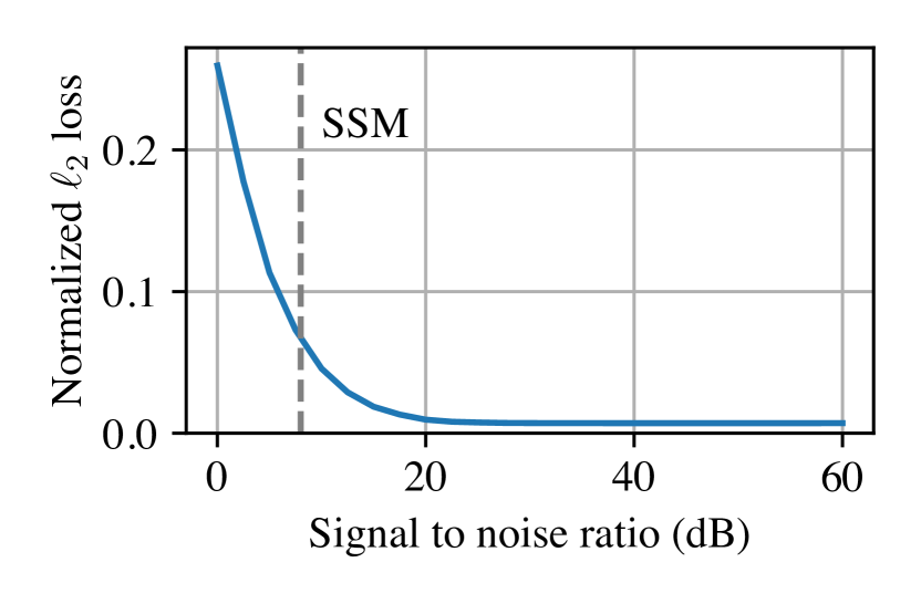
(a) Normalized $\ell_{2}$ loss versus SNR

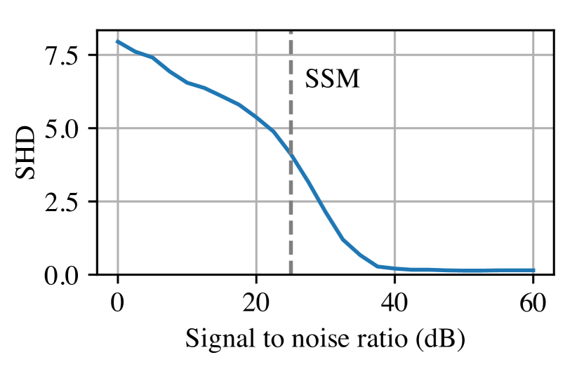
(b) SHD versus SNR

Figure 3: The performance of LSCALE-I under noisy scores with varying SNR for $n=5$ and $d=25$. The dashed vertical lines correspond to SNR values that correspond to the performance attained by SSM-VR.

8 Concluding Remarks

In this paper, we have proposed a score function-based CRL framework that uses stochastic interventions to learn latent causal representations and the latent causal graph underlying them. In this framework, by uncovering novel connections between score functions and CRL, we have established identifiability results for linear and general transformations without restricting the latent causal models, and designed LSCALE-I and GSCALE-I algorithms that achieve these identifiability guarantees.

There are several exciting directions for future work. Currently, we consider atomic interventions in which exactly one causal mechanism is altered in each interventional environment. Establishing the necessary and sufficient conditions for a set of multi-target interventional environments to suffice for perfect or partial identifiability is an important direction with practical implications. Next, we note that our LSCALE-I algorithm for linear transformations is agnostic to the intervention type and latent causal model, meaning that it can be used for both soft and hard interventions and different causal models. Designing similar universal CRL algorithms that can handle general transformations under different sizes and types of interventional environments is the ultimate goal for studying the identifiability of CRL from interventions. Finally, a missing component of existing CRL literature is the finite-sample analysis. Probabilistic identifiability results for a given number of interventional data samples can be useful, especially in applications where performing interventions is costly. Hence, it is an exciting future direction to infer partial causal information from a limited number of samples and knowledge about unseen interventions from available interventions.

Appendix

Table 6: Notation.

	$[n]$	:	$\{1,\dots,n\}$
	$\mathds{1}$	:	indicator function
ground-truth variables:	$\mathcal{G}$	:	latent causal graph over $Z$
	$\mathcal{G}_{\rm tc}$	:	transitive closure of $\mathcal{G}$
	$\mathcal{G}_{\rm tr}$	:	transitive reduction of $\mathcal{G}$
	${\rm{pa}}(i)$	:	parents of node $i$ in $\mathcal{G}$
	${\rm{ch}}(i)$	:	children of node $i$ in $\mathcal{G}$
	${\rm{an}}(i)$	:	ancestors of node $i$ in $\mathcal{G}$
	${\rm{de}}(i)$	:	descendants of node $i$ in $\mathcal{G}$
	$X$	:	$[X_{1},\dots,X_{d}]^{\top}$    observed random variables
	$Z$	:	$[Z_{1},\dots,Z_{n}]^{\top}$    latent random variables
	$Z_{{\rm{pa}}(i)}$	:	vector formed by $Z_{i}$ for all $i\in{\rm{pa}}(i)$
	$g$	:	true decoder
	$h$	:	a valid encoder
	$\mathcal{H}$	:	the set of valid encoders $h$
	$\mathbf{G}$	:	true linear decoder
	$\mathbf{H}$	:	a valid linear encoder
intervention notations:	$\mathcal{E}^{0}$	:	observational environment
	$\mathcal{E}$	:	$(\mathcal{E}^{1},\dots,\mathcal{E}^{n})$   first interventional environments
	$\tilde{\mathcal{E}}$	:	$(\tilde{\mathcal{E}}^{1},\dots,\tilde{\mathcal{E}}^{n})$   second interventional environments
	$I^{m}$	:	the intervened nodes in $\mathcal{E}^{m}$
	$\tilde{I}^{m}$	:	the intervened nodes in $\tilde{\mathcal{E}}^{m}$
	$\mathcal{I}$	:	the set of intervened nodes $(I^{1},\dots,I^{n})$
	$\tilde{\mathcal{I}}$	:	the set of intervened nodes $(\tilde{I}^{1},\dots,\tilde{I}^{n})$
statistical models:	$\hat{Z}(X)$	:	generic estimator of $Z$ given $X$
	$\hat{Z}(X;h)$	:	an auxiliary estimator of $Z$ given $X$ and encoder $h$
	$\hat{\mathcal{G}}$	:	estimate of $\mathcal{G}$
	$p,p^{m},\tilde{p}^{m}$	:	pdfs of $Z$ in $\mathcal{E}^{0}$, $\mathcal{E}^{m}$, and $\tilde{\mathcal{E}}^{m}$
	$p_{X},p_{X}^{m},\tilde{p}_{X}^{m}$	:	pdfs of $X$ in $\mathcal{E}^{0}$, $\mathcal{E}^{m}$, and $\tilde{\mathcal{E}}^{m}$
	$s,s^{m},\tilde{s}^{m}$	:	score functions of $Z$ in $\mathcal{E}^{0}$, $\mathcal{E}^{m}$, and $\tilde{\mathcal{E}}^{m}$
	$s_{X},s_{X}^{m},\tilde{s}_{X}^{m}$	:	score functions of $X$ in $\mathcal{E}^{0}$, $\mathcal{E}^{m}$, and $\tilde{\mathcal{E}}^{m}$
	$s_{\hat{Z}},s_{\hat{Z}}^{m},\tilde{s}_{\hat{Z}}^{m}$	:	score functions of $\hat{Z}$ in $\mathcal{E}^{0}$, $\mathcal{E}^{m}$, and $\tilde{\mathcal{E}}^{m}$ for encoder $h$
	$\hat{\rm{pa}}(i)$	:	parents of node $i$ in $\hat{\mathcal{G}}$
matrix notations:	$\mathbf{A}^{{\dagger}}$	:	Pseudo-inverse of matrix $\mathbf{A}$
	$\mathbf{A}_{i}$	:	row $i$ of matrix $\mathbf{A}$
	$\mathbf{A}_{i,j}$	:	entry of matrix $\mathbf{A}$ at row $i$ and column $j$
	$\mathbf{P}_{\pi}$	:	Permutation matrix associated with permutation $\pi$ of $[n]$
	$\mathcal{R}(f)$	:	$\dim(\operatorname{im}(f))$ for a function $f$
	$\mathcal{R}(\mathcal{F})$	:	$\dim(\operatorname{im}(\mathcal{F}))$ for a set of functions $\mathcal{F}$
	$\mathbf{D},\tilde{\mathbf{D}},\mathbf{D}_{\rm t}$	:	True score change matrices
	$\mathbf{D}(h),\tilde{\mathbf{D}}(h),\mathbf{D}_{\rm t}(h)$	:	Score change matrices under encoder $h$

Appendix A Proofs of Score Function Properties and Transformations

We start by providing the following facts that will be used repeatedly in the proofs.

Proposition 2

Consider two continuous functions $f,g:{\mathbb{R}}^{n}\to{\mathbb{R}}$. Then, for any $\alpha>0$,

$$\exists z\in{\mathbb{R}}^{n}\;\;f(z)\neq g(z)\quad\iff\quad{\mathbb{E}}\Big{[}\big{|}f(Z)-g(Z)\big{|}^{\alpha}\Big{]}\neq 0\ .$$ (73)

Specifically, for $\alpha=1$, we have

$$\exists z\in{\mathbb{R}}^{n}\;\;f(z)\neq g(z)\quad\iff\quad{\mathbb{E}}\Big{[}\big{|}f(Z)-g(Z)\big{|}\Big{]}\neq 0\ .$$ (74)

Proof: If there exists $z\in{\mathbb{R}}^{n}$ such that $f(z)\neq g(z)$, then $f(z)-g(z)$ is non-zero over a non-zero-measure set due to continuity. Then, ${\mathbb{E}}\big{[}|f(Z)-g(Z)|^{\alpha}\big{]}\neq 0$ since $p$ (pdf of $Z$) has full support. On the other direction, if $f(z)=g(z)$ for all $z\in{\mathbb{R}}^{n}$, then ${\mathbb{E}}\big{[}|f(Z)-g(Z)|^{\alpha}\big{]}=0$. This means that ${\mathbb{E}}\big{[}|f(Z)-g(Z)|^{\alpha}\big{]}\neq 0$ implies that there exists $z\in{\mathbb{R}}^{n}$ such that $f(z)\neq g(z)$.

A.1 Proof of Lemma 3

Our score-based methodology builds on the changes in score functions under interventions. For proving Lemma 3, we use the following intermediate result which formalizes the weakest possible requirement for a meaningful intervention and shows that it is a property of (i) hard interventions under any causal model, and (ii) additive noise model under either soft or hard interventions.

Lemma 14 (Interventional Regularity)

Causal mechanisms $p_{i}$ and $q_{i}$ of node $i$ are said to satisfy interventional regularity if

$$\exists z\in{\mathbb{R}}^{n}\;\;\mbox{such that}\quad\frac{\partial}{\partial z_{k}}\frac{q_{i}(z_{i}\mid z_{{\rm{pa}}(i)})}{p_{i}(z_{i}\mid z_{{\rm{pa}}(i)})}\neq 0\ ,\qquad\forall k\in{\rm{pa}}(i)\ .$$ (75)

Then, $p_{i}$ and $q_{i}$ satisfy interventional regularity if at least one of the following conditions is true:

1. The intervention is hard, i.e., $q_{i}(z_{i}\;|\;z_{{\rm{pa}}(i)})=q_{i}(z_{i})$.

2. The causal model is an additive noise model in which the pdfs of the noise variables are analytic.

Proof: See Appendix A.3.

Case (i) and Case (ii).

We give the proof for soft interventions on additive noise models, Case (i). We will use interventional regularity since Lemma 14 shows that it is satisfied for additive noise models. The proof for hard interventions, Case (ii), follows from similar arguments since interventional regularity is also satisfied for hard interventions by Lemma 14.

Proof of ${\mathbb{E}}\Big{[}\big{|}[s(Z)-s^{m}(Z)]_{i}\big{|}\Big{]}\neq 0\implies i\in\overline{{\rm{pa}}}(I^{m})$:

Let $\ell$ denote the node intervened in $\mathcal{E}^{m}$, i.e. $I^{m}=\ell$. Following (4) and (15), the latent scores $s(z)$ and $s^{m}(z)$ are decomposed as

$$s(z) =\nabla_{z}\log p_{\ell}(z_{\ell}\;|\;z_{{\rm{pa}}(\ell)})+\sum_{i\neq\ell}\nabla_{z}\log p_{i}(z_{i}\;|\;z_{{\rm{pa}}(i)})\ ,$$ (76)

$$\mbox{and}\quad s^{m}(z) =\nabla_{z}\log q_{\ell}(z_{\ell}\;|\;z_{{\rm{pa}}(\ell)})+\sum_{i\neq\ell}\nabla_{z}\log p_{i}(z_{i}\;|\;z_{{\rm{pa}}(i)})\ .$$ (77)

Hence, $s(z)$ and $s^{m}(z)$ differ in only the causal mechanism of node $\ell$. Next, we check the derivatives of $p_{\ell}(z_{\ell}\;|\;z_{{\rm{pa}}(\ell)})$ and $q_{\ell}(z_{\ell}\;|\;z_{{\rm{pa}}(\ell)})$ in their $i$-th coordinates. Note that these two depend on $Z$ only through $\{Z_{j}:\;j\in\overline{{\rm{pa}}}(\ell)\}$. Therefore, if $i\notin\overline{{\rm{pa}}}(\ell)$,

$$\partialderivative{z_{i}}\log p_{\ell}(z_{\ell}\;|\;z_{{\rm{pa}}(\ell)})=\partialderivative{z_{i}}\log q_{\ell}(z_{\ell}\;|\;z_{{\rm{pa}}(\ell)})=0\ ,$$ (78)

which indicates that if $i\notin\overline{{\rm{pa}}}(\ell)$, then $[s(z)]_{i}=[s^{m}(z)]_{i}$ for all $z$. This, equivalently, means that if ${\mathbb{E}}\big{[}\big{|}[s(Z)-s^{m}(Z)]_{i}\big{|}\big{]}\neq 0$, then $i\in\overline{{\rm{pa}}}({\ell})$.

Proof of $i\in\overline{{{\rm{pa}}}}(I^{m})\implies{\mathbb{E}}\Big{[}\big{|}[s(Z)-s^{m}(Z)]_{i}\big{|}\Big{]}\neq 0$:

Note that the two score functions $s$ and $s^{m}$ are equal in their coordinate $i\in\overline{\rm pa}(\ell)$ only if

$$0 =\frac{\partial\log q_{\ell}(z_{\ell}\mid z_{{\rm{pa}}(\ell)})}{\partial z_{i}}-\frac{\partial\log p_{\ell}(z_{\ell}\mid z_{{\rm pa}(\ell)})}{\partial z_{i}}=\frac{\partial}{\partial z_{i}}\log\frac{q_{\ell}(z_{\ell}\mid z_{{\rm{pa}}(i)})}{p_{\ell}(z_{\ell}\mid z_{{\rm{pa}}(\ell)})}\ .$$ (79)

However, (79) contradicts with interventional regularity. Therefore, if $i\in\overline{{\rm pa}}(\ell)$, $[s(z)_{i}]$ and $[s^{m}(z)]_{i}$ are not identical and by Proposition 2, ${\mathbb{E}}\big{[}\big{|}[s(Z)-s^{m}(Z)]_{i}\big{|}\big{]}\neq 0$.

Case (iii) Coupled environments.

Suppose that $I^{m}=\tilde{I}^{m}=\ell$. Following (16), we have

$$s^{m}(z) =\nabla_{z}\log q_{\ell}(z_{\ell})+\sum_{i\neq\ell}\nabla_{z}\log p_{i}(z_{i}\;|\;z_{{\rm{pa}}(i)})\ ,$$ (80)

$$\mbox{and}\quad\tilde{s}^{m}(z) =\nabla_{z}\log\tilde{q}_{\ell}(z_{\ell})+\sum_{i\neq\ell}\nabla_{z}\log p_{i}(z_{i}\;|\;z_{{\rm{pa}}(i)})\ .$$ (81)

Then, subtracting (81) from (80) and looking at $i$-th coordinate, we have

$$\big{[}s^{m}(z)-\tilde{s}^{m}(z)\big{]}_{i} =\dfrac{\partial\log q_{\ell}(z_{\ell})}{\partial z_{i}}-\dfrac{\partial\log\tilde{q}_{\ell}(z_{\ell})}{\partial z_{i}}\ .$$ (82)

If $i\neq\ell$, the right-hand side is zero and we have $\big{[}s^{m}(z)-\tilde{s}^{m}(z)\big{]}_{i}=0$ for all $z$. On the other hand, if $i=\ell$, since $q_{\ell}(z_{\ell})$ and $\tilde{q}_{\ell}(z_{\ell})$ are distinct, there exists $z\in{\mathbb{R}}^{n}$ such that $q_{\ell}(z_{\ell})\neq\tilde{q}_{\ell}(z_{\ell})$. Subsequently, by Proposition 2, we have ${\mathbb{E}}\big{[}\big{|}[s^{m}(Z)-\tilde{s}^{m}(Z)]_{i}\big{|}\big{]}\neq 0$.

Case (iv) Uncoupled environments.

Suppose that $I^{m}=\ell$ and $\tilde{I}^{m}=j$, and $\ell\neq j$. Following (16), we have

$$s^{m}(z) =\nabla_{z}\log q_{\ell}(z_{\ell})+\nabla_{z}\log p_{j}(z_{j}\;|\;z_{{\rm{pa}}(j)})+\sum_{k\in[n]\setminus\{\ell,j\}}\nabla_{z}\log p_{k}(z_{k}\;|\;z_{{\rm{pa}}(k})\ ,$$ (83)

$$\mbox{and}\quad\tilde{s}^{m}(z) =\nabla_{z}\log q_{j}(z_{j})+\nabla_{z}\log p_{\ell}(z_{\ell}\;|\;z_{{\rm{pa}}(\ell)})+\sum_{k\in[n]\setminus\{\ell,j\}}\nabla_{z}\log p_{k}(z_{k}\;|\;z_{{\rm{pa}}(k)})\ .$$ (84)

Then, subtracting (84) from (83) we have

$$s^{m}(z)-\tilde{s}^{m}(z) =\;\nabla_{z}\log q_{\ell}(z_{\ell})+\nabla_{z}\log p_{j}(z_{j}\;|\;z_{{\rm{pa}}(j)})-\nabla_{z}\log q_{j}(z_{j})-\nabla_{z}\log p_{\ell}(z_{\ell}\;|\;z_{{\rm{pa}}(\ell)})\ .$$ (85)

Scrutinizing the $i$-th coordinate, we have

$$\big{[}s^{m}(z)-\tilde{s}^{m}(z)\big{]}_{i} =\dfrac{\partial\log q_{\ell}(z_{\ell})}{\partial z_{i}}+\dfrac{\partial\log p_{j}(z_{j}\;|\;z_{{\rm{pa}}(j)})}{\partial z_{i}}-\dfrac{\partial\log q_{j}(z_{j})}{\partial z_{i}}-\dfrac{\partial\log p_{\ell}(z_{\ell}\;|\;z_{{\rm{pa}}(\ell)})}{\partial z_{i}}\ .$$ (86)

Proof of ${\mathbb{E}}\Big{[}\big{|}[s^{m}(Z)-\tilde{s}^{m}(Z)\big{]}_{i}\big{|}\Big{]}\neq 0\ \implies i\in\overline{{{\rm{pa}}}}(\ell,j)$:

Suppose that $i\notin\overline{{\rm{pa}}}({\ell},j)$. Then, none of the terms in the RHS of (86) is a function of $z_{i}$. Therefore, all the terms in the RHS of (86) are zero, and we have $\big{[}s^{m}(z)-\tilde{s}^{m}(z)\big{]}_{i}=0$ for all $z$. By Proposition 2, ${\mathbb{E}}\big{[}\big{|}[s^{m}(Z)-\tilde{s}^{m}(Z)]_{i}\big{|}\big{]}=0$. This, equivalently, means that if ${\mathbb{E}}\big{[}\big{|}[s^{m}(Z)-\tilde{s}^{m}(Z)]_{i}\big{|}\big{]}\neq 0$, then $i\in\overline{{\rm{pa}}}({\ell},j)$.

Proof of ${\mathbb{E}}\Big{[}\big{|}[s^{m}(Z)-\tilde{s}^{m}(Z)]_{i}\big{|}\Big{]}\neq 0\impliedby i\in\overline{{{\rm{pa}}}}(\ell,j)$:

We prove it by contradiction. Assume that $\big{[}s^{m}(z)-\tilde{s}^{m}(z)\big{]}_{i}=0$ for all $z$. Without loss of generality, let $\ell\notin\overline{{\rm{pa}}}(j)$.

 If $i=\ell$.

In this case, (86) is simplified to

$$0=\big{[}s^{m}(z)-\tilde{s}^{m}(z)\big{]}_{\ell}=\dfrac{\partial\log q_{\ell}(z_{\ell})}{\partial z_{\ell}}-\dfrac{\partial\log p_{\ell}(z_{\ell}\;|\;z_{{\rm{pa}}(\ell)})}{\partial z_{\ell}}\ .$$ (87)

If $\ell$ is a root node, i.e., ${\rm{pa}}(\ell)=\emptyset$, (87) implies that $(\log q_{\ell})^{\prime}(z_{\ell})=(\log p_{\ell})^{\prime}(z_{\ell})$ for all $z_{\ell}$. Integrating, we get $p_{\ell}(z_{\ell})=\alpha q_{\ell}(z_{\ell})$ for some constant $\alpha$. Since both $p_{\ell}$ and $q_{\ell}$ are pdfs, they both integrate to one, implying $\alpha=1$ and $p_{\ell}(z_{\ell})=q_{\ell}(z_{\ell})$, which contradicts the premise that observational and interventional mechanisms are distinct. If $\ell$ is not a root node, consider some $k\in{\rm{pa}}(\ell)$. Then, taking the derivative of (87) with respect to $z_{k}$, we have

$$0=\dfrac{\partial^{2}\log p_{\ell}(z_{\ell}\;|\;z_{{\rm{pa}}(\ell)})}{\partial z_{\ell}\partial z_{k}}\ .$$ (88)

Recall the equation $Z_{\ell}=f_{\ell}(Z_{{\rm{pa}}(\ell)})+N_{\ell}$ for additive noise models specified in (7). Denote the pdf of the noise term $N_{\ell}$ by $p_{N}$. Then, the conditional pdf $p_{\ell}(z_{\ell}\;|\;z_{{\rm{pa}}(\ell)})$ is given by $p_{\ell}(z_{\ell}\;|\;z_{{\rm{pa}}(\ell)})=p_{N}(z_{\ell}-f_{\ell}(z_{{\rm{pa}}(\ell)}))$. Denoting the score function of $p_{N}$ by $r_{p}$,

$$r_{p}(u)\triangleq\dfrac{\rm d}{{\rm d}u}\log p_{N}(u)\ ,$$ (89)

we have

$$\dfrac{\partial\log p_{\ell}(z_{\ell}\;|\;z_{{\rm{pa}}(\ell)})}{\partial z_{\ell}}=\dfrac{\partial\log p_{N}(z_{\ell}-f_{\ell}(z_{{\rm{pa}}(\ell)}))}{\partial z_{\ell}}=r_{p}(z_{\ell}-f_{\ell}(z_{{\rm{pa}}(\ell)}))\ .$$ (90)

Substituting this into (88), we obtain

$$0 =\dfrac{\partial r_{p}\big{(}z_{\ell}-f_{\ell}(z_{{\rm{pa}}(\ell)})\big{)}}{\partial z_{k}}=-\dfrac{\partial f_{\ell}(z_{{\rm{pa}}(\ell)})}{\partial z_{k}}\cdot r_{p}^{\prime}\big{(}z_{\ell}-f_{\ell}(z_{{\rm{pa}}(\ell)})\big{)}\ ,\quad\forall z\in{\mathbb{R}}^{n}\ .$$ (91)

Since $k$ is a parent of $\ell$, there exists a fixed $Z_{{\rm{pa}}(\ell)}=z_{{\rm{pa}}(\ell)}^{*}$ realization for which $\partial f_{\ell}(z_{{\rm{pa}}(\ell)}^{*})/\partial z_{k}$ is non-zero. Otherwise, $f_{\ell}(z_{{\rm{pa}}(\ell)})$ would not be sensitive to $z_{k}$ which is contradictory to $k$ being a parent of $\ell$. Note that $Z_{\ell}$ can vary freely after fixing $Z_{{\rm{pa}}(\ell)}$. Therefore, for (91) to hold, the derivative of $r_{p}$ must always be zero. However, the score function of a valid pdf with full support cannot be constant. Therefore, $\big{[}s^{m}(z)_{i}-\tilde{s}^{m}(z)\big{]}_{i}$ is not always zero, and we have ${\mathbb{E}}\big{[}\big{|}[s^{m}(Z)-\tilde{s}^{m}(Z)]_{i}\big{|}\big{]}\neq 0$.

 If $i\neq\ell$

. In this case, (86) is simplified to

$$0=\big{[}s^{m}(z)-\tilde{s}^{m}(z)\big{]}_{i}=\dfrac{\partial\log p_{j}(z_{j}\;|\;z_{{\rm{pa}}(j)})}{\partial z_{i}}-\dfrac{\partial\log q_{j}(z_{j})}{\partial z_{i}}-\dfrac{\partial\log p_{\ell}(z_{\ell}\;|\;z_{{\rm{pa}}(\ell)})}{\partial z_{i}}\ .$$ (92)

We investigate case by case and reach a contradiction for each case. First, suppose that $i\notin{\rm{pa}}({\ell})$. Then, we have $i\in\overline{{\rm{pa}}}(j)$, and (92) becomes

$$0=\big{[}s^{m}(z)-[\tilde{s}^{m}(z)\big{]}_{i}=\dfrac{\partial\log p_{j}(z_{j}\;|\;z_{{\rm{pa}}(j)})}{\partial z_{i}}-\dfrac{\partial\log q_{j}(z_{j})}{\partial z_{i}}\ .$$ (93)

If $i=j$, the impossibility of (93) directly follows from the impossibility of (87). The remaining case is $i\in{\rm{pa}}(j)$. In this case, taking the derivative of the right-hand side of (93) with respect to $z_{j}$, we obtain

$$0=\dfrac{\partial^{2}\log p_{j}(z_{j}\;|\;z_{{\rm{pa}}(j)})}{\partial z_{i}\partial z_{j}}\ ,$$ (94)

which is a realization of (88) for $i\in{\rm{pa}}(j)$ and $j$ in place of $k\in{\rm{pa}}(\ell)$ and $\ell$, which we proved to be impossible in $i=\ell$ case. Therefore, $i\notin{\rm{pa}}(\ell)$ is not viable. Finally, suppose that $i\in{\rm{pa}}({\ell})$. Then, taking the derivative of the right-hand side of (92) with respect to $z_{\ell}$, we obtain

$$0=\dfrac{\partial^{2}\log p_{\ell}(z_{\ell}\;|\;z_{{\rm{pa}}(\ell)})}{\partial z_{i}\partial z_{\ell}}\ ,$$ (95)

which is again a realization of (88) for $k=i$, which we proved to be impossible.

Hence, we showed that $\big{[}s^{m}(z)-\tilde{s}^{m}(z)\big{]}_{i}$ cannot be zero for all $z$ values. Then, by Proposition 2 we have ${\mathbb{E}}\big{[}\big{|}[s^{m}(Z)-\tilde{s}^{m}(Z)]_{i}\big{|}\big{]}\neq 0$, and the proof is concluded.

A.2 Proof of Lemma 4

Let us recall the setting. Consider random vectors $Y_{1},Y_{2}\in{\mathbb{R}}^{r}$ and $W_{1}$, $W_{2}\in{\mathbb{R}}^{s}$ that are related through $Y_{1}=f(W_{1})$ and $Y_{2}=f(W_{2})$ such that $r\geq s$, probability measures of $W_{1},W_{2}$ are absolutely continuous with respect to the $s$-dimensional Lebesgue measure and $f:{\mathbb{R}}^{s}\to{\mathbb{R}}^{r}$ is an injective and continuously differentiable function.

In this setting, the realizations of $W_{1}$ and $Y_{1}$, and that of $W_{2}$ and $Y_{2}$, are related through $y=f(w)$. Since $f$ is injective and continuously differentiable, volume element ${\rm d}w$ in ${\mathbb{R}}^{s}$ gets mapped to $\left|\det([J_{f}(w)]^{\top}\cdot J_{f}(w))\right|^{1/2}\ {\rm d}w$ on $\operatorname{im}(f)$. Since $W_{1}$ has density $p_{W_{1}}$ absolutely continuous with respect to the $s$-dimensional Lebesgue measure, using the area formula (Boothby, 2003), we can define a density for $Y_{1}$, denoted by $p_{Y_{1}}$, supported only on manifold $\mathcal{M}\triangleq\operatorname{im}(f)$ which is absolutely continuous with respect to the $s$-dimensional Hausdorff measure:

$$p_{Y_{1}}(y)=p_{W_{1}}(w)\cdot\left|\det([J_{f}(w)]^{\top}\cdot J_{f}(w))\right|^{-1/2}\ ,\quad\mbox{where}\quad y=f(w)\ .$$ (96)

Densities $p_{Y_{2}}$ and $p_{W_{2}}$ of $Y_{2}$ and $W_{2}$ are related similarly. Subsequently, score functions of $\{W_{1},W_{2}\}$ and $\{Y_{1},Y_{2}\}$ are specified similarly to (9) and (14), respectively. Denote the Jacobian matrix of $f$ at point $w\in{\mathbb{R}}^{s}$ by $J_{f}(w)$, which is an $r\times s$ matrix with entries given by

$$\big{[}J_{f}(w)\big{]}_{i,j}=\partialderivative{\big{[}f(w)\big{]}_{i}}{w_{j}}=\partialderivative{y_{i}}{w_{j}}\ ,\quad\forall i\in[r]\;,j\in[s]\ .$$ (97)

Next, consider a function $\phi\colon\mathcal{M}\to{\mathbb{R}}$. Since the domain of $\phi$ is a manifold, its differential, denoted by $D\phi$, is defined according to (12). By noting $y=f(w)$, we can also differentiate $\phi$ with respect to $w\in{\mathbb{R}}^{s}$ as (Simon, 2014, p. 57)

$$\nabla_{w}\phi(y)=\nabla_{w}(\phi\circ f)(w)=\big{[}J_{f}(w)\big{]}^{\top}\cdot D\phi(y)\ .$$ (98)

Next, given the identities in (96) and (98), we find the relationship between score functions of $W_{1}$ and $Y_{1}$ as follows.

$$s_{W_{1}}(w) =\nabla_{w}\log p_{W_{1}}(w)$$ (99)

$${=}\nabla_{w}\log p_{Y_{1}}(y)+\nabla_{w}\log\left|\det([J_{f}(w)]^{\top}\cdot J_{g}(w))\right|^{1/2}$$ (100)

$${=}\big{[}J_{f}(w)\big{]}^{\top}\cdot D\log p_{Y_{1}}(y)+\nabla_{w}\log\left|\det([J_{f}(w)]^{\top}\cdot J_{f}(w))\right|^{1/2}$$ (101)

$$=\big{[}J_{f}(w)\big{]}^{\top}\cdot s_{Y_{1}}(y)+\nabla_{w}\log\left|\det([J_{f}(w)]^{\top}\cdot J_{f}(w))\right|^{1/2}\ .$$ (102)

Following the similar steps that led to (102) for $W_{2}$ and $Y_{2}$, we obtain

$$s_{W_{2}}(w) =\big{[}J_{f}(w)\big{]}^{\top}\cdot s_{Y_{2}}(y)+\nabla_{w}\log\left|\det([J_{f}(w)]^{\top}\cdot J_{f}(w))\right|^{1/2}\ .$$ (103)

Subtracting (103) from (102), we obtain the desired result

$$s_{W_{1}}(w)-s_{W_{2}}(w)=\big{[}J_{f}(w)\big{]}^{\top}\cdot\big{[}s_{Y_{1}}(y)-s_{Y_{2}}(y)\big{]}\ .$$ (104)

Corollary 1

In Lemma 4, if $f$ is a linear transform, that is $Y=\mathbf{F}\cdot W$ for a full-rank matrix $\mathbf{F}\in{\mathbb{R}}^{r\times s}$, then the score functions of $Y$ and $W$ are related through $s_{W}(w)=\mathbf{F}^{\top}\cdot s_{Y}(y)$, where $y=\mathbf{F}\cdot w$.

Proof: For the given linear transform, we have $J_{f}(w)=\mathbf{F}$, which is independent of $w$. Then, in the proof of Lemma 4, (102) reduces to $s_{W}(w)=\mathbf{F}^{\top}\cdot s_{Y}(y)$. Finally, we note that the score difference of $Y$ can be similarly written in terms of the score difference of $W$.

Corollary 2

Under the same setting and the assumptions as Lemma 4, we have

$$s_{Y_{1}}(y)-s_{Y_{2}}(y)=\Big{[}\big{[}J_{f}(w)\big{]}^{{\dagger}}\Big{]}^{\top}\cdot\big{[}s_{W_{1}}(w)-s_{W_{2}}(w)\big{]}\ ,\quad\mbox{where}\;\;y=f(w)\ .$$ (105)

Proof: Multiplying (104) from left with $\big{[}[J_{f}(w)]^{{\dagger}}\big{]}^{\top}$, we obtain

$$\Big{[}\big{[}J_{f}(w)\big{]}^{{\dagger}}\Big{]}^{\top}\cdot\big{[}s_{W_{1}}(w)-s_{W_{2}}(w)\big{]}=\Big{[}\big{[}J_{f}(w)\big{]}^{{\dagger}}\Big{]}^{\top}\cdot\big{[}J_{f}(w)\big{]}^{\top}\cdot\big{[}s_{Y_{1}}(y)-s_{Y_{2}}(y)\big{]}\ .$$ (106)

Note that

$$\Big{[}\big{[}J_{f}(w)\big{]}^{{\dagger}}\Big{]}^{\top}\cdot\big{[}J_{f}(w)\big{]}^{\top}=J_{f}(w)\cdot\big{[}J_{f}(w)\big{]}^{{\dagger}}\ .$$ (107)

Note that, by properties of the Moore-Penrose inverse, for any matrix $\mathbf{A}$, we have $\mathbf{A}\cdot\mathbf{A}^{{\dagger}}\cdot\mathbf{A}=\mathbf{A}$. This means that $\mathbf{A}\cdot\mathbf{A}^{{\dagger}}$ acts as a left identity for vectors in the column space of $\mathbf{A}$. By definition, $s_{Y_{1}}$ and $s_{Y_{2}}$ have values in $T_{w}\operatorname{im}(f)$, the tangent space of the image manifold $f$ at point $w$. This space is equal to the column space of matrix $J_{f}(w)$. Therefore, $J_{f}(w)\cdot[J_{f}(w)]^{{\dagger}}$ acts as a left identity for $s_{Y_{1}}(y)$ and $s_{Y_{2}}(y)$, and we have

$$J_{f}(w)\cdot\big{[}J_{f}(w)\big{]}^{{\dagger}}\cdot\big{[}s_{Y_{1}}(y)-s_{Y_{2}}(y)\big{]}=s_{Y_{1}}(y)-s_{Y_{2}}(y)\ .$$ (108)

Substituting (107) and (108) into (106) completes the proof.

A.3 Proof of Lemma 14

We will prove that causal mechanisms $p_{i}$ and $q_{i}$ satisfy interventional regularity for (i) hard interventions and (ii) additive noise models. To this end, we first define

$$\psi(z_{i},z_{{\rm{pa}}(i)})\triangleq\frac{q_{i}(z_{i}\mid z_{{\rm{pa}}(i)})}{p_{i}(z_{i}\mid z_{{\rm{pa}}(i)})}\ .$$ (109)

We start by showing that $\psi(z_{i},z_{{\rm{pa}}(i)})$ varies with $z_{i}$. We prove it by contradiction. Assume the contrary, i.e., let $\psi(z_{i},z_{{\rm{pa}}(i)})=\psi(z_{{\rm{pa}}(i)})$. By rearranging (109) we have

$$q_{i}(z_{i}\mid z_{{\rm{pa}}(i)})=\psi(z_{{\rm{pa}}(i)})\,p_{i}(z_{i}\mid z_{{\rm{pa}}(i)})\ .$$ (110)

Fix a realization of $z_{{\rm{pa}}(i)}=z_{{\rm{pa}}(i)}^{*}$ and integrate both sides of (110) with respect to $z_{i}$. Since both $p_{i}$ and $q_{i}$ are pdfs, we have

$$1 =\int_{{\mathbb{R}}}q_{i}(z_{i}\mid z_{{\rm{pa}}(i)}^{*})\,\differential z_{i}=\int_{{\mathbb{R}}}\psi(z_{{\rm{pa}}(i)}^{*})\,p_{i}(z_{i}\mid z_{{\rm{pa}}(i)}^{*})\mathrm{d}{z_{i}}\differential z_{i}$$ (111)

$$=\psi(z_{{\rm{pa}}(i)}^{*})\int_{{\mathbb{R}}}p_{i}(z_{i}\mid z_{{\rm{pa}}(i)}^{*})\differential z_{i}$$ (112)

$$=\psi(z_{{\rm{pa}}(i)}^{*})\ .$$ (113)

This identity implies that $p_{i}(z_{i}\mid z_{{\rm{pa}}(i)}^{*})=q_{i}(z_{i}\mid z_{{\rm{pa}}(i)}^{*})$ for any arbitrary realization $z_{{\rm{pa}}(i)}^{*}$. This contradicts the premise that observational and interventional distributions are distinct. As a result, to check if a model satisfies interventional regularity for node $i$, it suffices to investigate whether the function $\psi$ is not invariant with respect to $z_{k}$ for $k\in{\rm{pa}}(i)$. To this end, from (109) we know that $\psi(z_{i},z_{{\rm{pa}}(i)})$ varies with $z_{k}$ if and only if

$$\frac{\partial}{\partial z_{i}}\log\psi(z_{i},z_{{\rm{pa}}(i)})=\frac{\partial q_{i}(z_{i}\mid z_{{\rm{pa}}(i)})}{\partial z_{i}}\cdot\frac{1}{q_{i}(z_{i}\mid z_{{\rm{pa}}(i)})}-\frac{\partial p_{i}(z_{i}\mid z_{{\rm{pa}}(i)})}{\partial z_{i}}\cdot\frac{1}{p_{i}(z_{i}\mid z_{{\rm{pa}}(i)})}\neq 0\ .$$ (114)

Next, we investigate the sufficient conditions listed in the Lemma 14.

A.3.1 Hard Interventions

Under hard interventions, note that for any $k\in{\rm{pa}}(i)$,

$$\frac{\partial}{\partial z_{k}}p_{i}(z_{i}\mid z_{{\rm{pa}}(i)})\neq 0\ ,\quad\mbox{and}\quad\frac{\partial}{\partial z_{k}}q_{i}(z_{i})=0\ .$$ (115)

Then, it follows directly from (114) that

$$\frac{\partial}{\partial z_{k}}\log\psi(z_{i},z_{{\rm{pa}}(i)}) =\underset{=\,0}{\underbrace{\frac{\partial q_{i}(z_{i})}{\partial z_{k}}}}\cdot\frac{1}{q_{i}(z_{i})}-\underset{\neq\,0}{\underbrace{\frac{\partial p_{i}(z_{i}\mid z_{{\rm{pa}}(i)})}{\partial z_{k}}}}\cdot\frac{1}{p_{i}(z_{i}\mid z_{{\rm{pa}}(i)})}\neq 0\ .$$ (116)

Thus, hard interventions on any latent causal model satisfy interventional regularity.

A.3.2 Additive Noise Models

The additive noise model for node $i$ is given by

$$Z_{i} =f_{i}(Z_{{\rm{pa}}(i)})+N_{i}\ ,$$ (117)

as specified in (7). When node $i$ is soft intervened, $Z_{i}$ is generated according to

$$Z_{i} =\bar{f}_{i}(Z_{{\rm{pa}}(i)})+\bar{N}_{i}\ ,$$ (118)

in which $\bar{f}_{i}$ and $\bar{N}_{i}$ specify the interventional mechanism for node $i$. Then, denoting the pdfs of $N_{i}$ and $\bar{N}_{i}$ by $p_{N}$ and $q_{N}$, respectively, (117) and (118) imply that

$$p_{i}(z_{i}\mid z_{{\rm{pa}}(i)})=p_{N}\big{(}z_{i}-f_{i}(z_{{\rm{pa}}(i)})\big{)}\ ,\quad\mbox{and}\quad q_{i}(z_{i}\mid z_{{\rm{pa}}(i)})=q_{N}\big{(}z_{i}-\bar{f}_{i}(z_{{\rm{pa}}(i)})\big{)}\ .$$ (119)

Denote the score functions associated with $p_{N}$ and $q_{N}$ by

$$r_{p}(u)\triangleq\frac{{\rm d}}{{\rm d}u}\log p_{N}(u)=\frac{p_{N}^{\prime}(u)}{p_{N}(u)}\ ,\quad\mbox{and}\quad r_{q}(u)\triangleq\frac{{\rm d}}{{\rm d}u}\log q_{N}(u)=\frac{q_{N}^{\prime}(u)}{q_{N}(u)}\ .$$ (120)

We will prove that (114) holds by contradiction. Assume the contrary and let

$$\frac{\partial q_{i}(z_{i}\mid z_{{\rm{pa}}(i)})}{\partial z_{k}}\cdot\frac{1}{q_{i}(z_{i}\mid z_{{\rm{pa}}(i)})}=\frac{\partial p_{i}(z_{i}\mid z_{{\rm{pa}}(i)})}{\partial z_{k}}\cdot\frac{1}{p_{i}(z_{i}\mid z_{{\rm{pa}}(i)})}\ .$$ (121)

From (119) and (120), for the numerators in (121) we have,

$$\frac{\partial p_{i}(z_{i}\mid z_{{\rm{pa}}(i)})}{\partial z_{k}} =-\frac{\partial f_{i}(z_{{\rm{pa}}(i)})}{\partial z_{k}}\cdot p_{N}^{\prime}\big{(}z_{i}-f_{i}(z_{{\rm{pa}}(i)})\big{)}\ ,$$ (122)

$$\mbox{and}\quad\frac{\partial q_{i}(z_{i}\mid z_{{\rm{pa}}(i)})}{\partial z_{k}} =-\frac{\partial\bar{f}_{i}(z_{{\rm{pa}}(i)})}{\partial z_{k}}\cdot q_{N}^{\prime}\big{(}z_{i}-\bar{f}_{i}(z_{{\rm{pa}}(i)})\big{)}\ .$$ (123)

Hence, the identity in (121) can be written as

$$\frac{\partial f_{i}(z_{{\rm{pa}}(i)})}{\partial z_{k}}\cdot r_{p}\big{(}z_{i}-f_{i}(z_{{\rm{pa}}(i)})\big{)} =\frac{\partial\bar{f}_{i}(z_{{\rm{pa}}(i)})}{\partial z_{k}}\cdot r_{q}\big{(}z_{i}-\bar{f}_{i}(z_{{\rm{pa}}(i)})\big{)}\ .$$ (124)

Define $n_{i}$ and $\bar{n}_{i}$ as the realizations of $N_{i}$ and $\bar{N}_{i}$ when $Z_{i}=z_{i}$ and $Z_{{\rm{pa}}(i)}=z_{{\rm{pa}}(i)}$. By defining $\delta(z_{{\rm{pa}}(i)})\triangleq f_{i}(z_{{\rm{pa}}(i)})-\bar{f}_{i}(z_{{\rm{pa}}(i)})$, we have $\bar{n}_{i}=n_{i}+\delta(z_{{\rm{pa}}(i)})$. Then, (124) can rewritten as

$$\frac{\partial f_{i}(z_{{\rm{pa}}(i)})}{\partial z_{k}}\cdot r_{p}(n_{i}) =\frac{\partial\bar{f}_{i}(z_{{\rm{pa}}(i)})}{\partial z_{k}}\cdot r_{q}(n_{i}+\delta(z_{{\rm{pa}}(i)}))\ .$$ (125)

Note that $\frac{\partial f_{i}(z_{{\rm{pa}}(i)})}{\partial z_{k}}$ is a non-zero continuous function. Hence, there exists an interval $\Phi\subseteq{\mathbb{R}}^{|{\rm{pa}}(i)|}$ over which $\frac{\partial f_{i}(z_{{\rm{pa}}(i)})}{\partial z_{k}}\neq 0$. Likewise, $r_{p}(n_{i})$ cannot be constantly zero over all possible intervals $\Omega\subseteq{\mathbb{R}}$. This is because otherwise, it would have to necessarily be a constant zero function (since it is analytic), which is an invalid score function. Hence, there exists an open interval $\Omega\subseteq\mathbb{R}$ over which $r_{p}(n_{i})$ is non-zero for all $n_{i}\in\Omega$. Then, we can rearrange (125) as

$$\frac{r_{p}(n_{i})}{r_{q}(n_{i}+\delta(z_{{\rm{pa}}(i)}))} =\frac{\frac{\partial\bar{f}_{i}(z_{{\rm{pa}}(i)})}{\partial z_{k}}}{\frac{\partial f_{i}(z_{{\rm{pa}}(i)})}{\partial z_{k}}}\ ,\quad\forall(n_{i},z_{{\rm{pa}}(i)})\in\Omega\times\Phi\ .$$ (126)

Note that the RHS of (126) is not a function of $n_{i}$. Then, taking the derivative of both sides with respect to $n_{i}$, we get

$$\frac{r_{p}^{\prime}(n_{i})}{r_{p}(n_{i})} =\frac{r_{q}^{\prime}(n_{i}+\delta(z_{{\rm{pa}}(i)}))}{r_{q}(n_{i}+\delta(z_{{\rm{pa}}(i)}))}\ .$$ (127)

In the next step, we show that $\delta$ is not a constant function. We prove this by contradiction. Suppose that $\delta(z_{{\rm{pa}}(i)})=\delta^{*}$ is a constant function. Then, the gradients of $f_{i}$ and $\bar{f}_{i}$ are equal. From (126), this implies that

$$r_{p}(n_{i}) =r_{q}(n_{i}+\delta^{*})\ ,\quad\forall n_{i}\in\Omega\ .$$ (128)

Since $r_{p}(n_{i})$ and $r_{q}(n_{i}+\delta^{*})$ are analytic functions that agree on an open interval of ${\mathbb{R}}$, they are equal for all $n_{i}\in{\mathbb{R}}$. This implies that $p_{N}(n_{i})=\eta q_{N}(n_{i}+\delta^{*})$ for some constant $\eta\in{\mathbb{R}}$. Since $p_{N}$ and $q_{N}$ are pdfs, $\eta=1$ is the only choice that maintains $p_{N}$ and $q_{N}$ are pdfs. Therefore, $p_{N}(n_{i})=q_{N}(n_{i}+\delta^{*})$. However, using (119), this implies that $p_{i}(z_{i}\mid z_{{\rm{pa}}(i)})=q_{i}(z_{i}\mid z_{{\rm{pa}}(i)})$, which contradicts the premise that an intervention changes the causal mechanism of target node $i$. Therefore $\delta$ is a continuous, non-constant function, and its image over $z_{{\rm{pa}}(i)}\in\Phi$ includes an open interval $\Theta\subseteq{\mathbb{R}}$. With this result in mind, we return to (127). Consider a fixed realization $n_{i}=n_{i}^{*}$ and denote the value of the left-hand side (LHS) for $n_{i}^{*}$ by $\alpha$. By defining $u\triangleq\delta(z_{{\rm{pa}}(i)})$, we get

$$\alpha =\frac{r_{q}^{\prime}(n_{i}^{*}+u)}{r_{q}(n_{i}^{*}+u)}\ ,\qquad\forall u\in\Theta\ .$$ (129)

This is only possible if $r_{q}$ is an exponential function, i.e., $r_{q}(u)=k_{1}\exp(\alpha u)$ over interval $u\in\Theta$. Since $r_{q}$ is an analytic function, it is, therefore, exponential over entire ${\mathbb{R}}$. Then, the associated pdf must have the form $q_{N}(u)=k_{2}\exp((k_{1}/\alpha)\exp(\alpha u))$. However, the integral of this function over the entire domain ${\mathbb{R}}$ diverges. Hence, it is not a valid pdf, rendering a contradiction. Hence, the additive noise model satisfies interventional regularity.

Appendix B Proofs of the Results for Linear Transformations

B.1 Proof of Lemma 5

Consider environment $\mathcal{E}^{m}$ and denote the intervened node by $\ell=I^{m}$. Lemma 3(i) and Lemma 3(ii) imply that, for any $m\in[n]$, the image of the function $(s-s^{m})$ contains a vector $z\in{\mathbb{R}}^{n}$ for which $z_{\ell}\neq 0$ and $z_{j}=0$ for $j\notin\overline{{\rm{pa}}}(\ell)$. Since $(Z_{1},\dots,Z_{n})$ are topologically ordered, this implies $z_{j}=0$ for $j\geq(\ell+1)$. Then, for different values of $m$, these specified vectors are linearly independent. Hence, $\operatorname{im}(\{s-s^{m}:m\in\mathcal{A}\})$ contains at least $|\mathcal{A}|$ linearly independent vectors and we have

$$\mathcal{R}\big{(}\{s-s^{m}:m\in\mathcal{A}\}\big{)}\geq|\mathcal{A}|\ .$$ (130)

On the other hand, using Lemma 3, the term $s(Z)-s^{m}(Z)$ can have non-zero entries only at the coordinates $\overline{{\rm{pa}}}(\ell)$. Therefore, in any vector in $\operatorname{im}(\{s-s^{m}:m\in\mathcal{A}\})$, the $j$-th coordinate is zero if $j\notin\overline{{\rm{pa}}}\big{(}I^{\mathcal{A}}\big{)}$. Subsequently, we have

$$\mathcal{R}\big{(}\{s-s^{m}:m\in\mathcal{A}\}\big{)}\leq\big{|}\overline{{\rm{pa}}}\big{(}I^{\mathcal{A}}\big{)}\big{|}\ .$$ (131)

Finally, if $I^{\mathcal{A}}$ is ancestrally closed, we have $\overline{{\rm{pa}}}\big{(}I^{\mathcal{A}}\big{)}=I^{\mathcal{A}}$. This implies that the inequalities in (130) and (131) hold with equality and we have

$$\mathcal{R}\big{(}\{s-s^{m}:m\in\mathcal{A}\}\big{)}=|\mathcal{A}|=\big{|}\overline{{\rm{pa}}}\big{(}I^{\mathcal{A}}\big{)}\big{|}\ .$$ (132)

B.2 Proof of Lemma 6

We consider a set $\mathcal{A}$ for which $I^{\mathcal{A}}$ is ancestrally closed, i.e., ${\rm{an}}(I^{\mathcal{A}})\subseteq I^{\mathcal{A}}$, and consider the score function differences $\big{\{}s-s^{m}:m\in\mathcal{A}\setminus\{k\}\big{\}}$ for some $k\in\mathcal{A}$. First, we use Lemma 5 to show that the rank of the image of these functions is either $|\mathcal{A}|$ or $|\mathcal{A}|-1$. Note that $\overline{{\rm{pa}}}\big{(}I^{\mathcal{A}}\big{)}=\overline{{\rm{pa}}}(I^{\mathcal{A}\setminus\{k\}})\cup\overline{{\rm{pa}}}(I^{k})$. Subsequently, since $I^{\mathcal{A}}$ is ancestrally closed, we have

$$\big{|}\overline{{\rm{pa}}}\big{(}I^{\mathcal{A}\setminus\{k\}}\big{)}\big{|}\leq\big{|}\overline{{\rm{pa}}}\big{(}I^{\mathcal{A}}\big{)}\big{|}=\big{|}I^{\mathcal{A}}\big{|}=|\mathcal{A}|\ .$$ (133)

Then, using Lemma 5, we have

$$|\mathcal{A}|\geq\mathcal{R}\Big{(}\big{\{}s-s^{m}:m\in\mathcal{A}\setminus\{k\}\big{\}}\Big{)}\geq|\mathcal{A}|-1\ .$$ (134)

Next, consider two cases as follows.

Case (i): $I^{k}$ does not have a child in $I^{\mathcal{A}}$.

In this case, $I^{\mathcal{A}\setminus\{k\}}$ is ancestrally closed, which implies

$$\big{|}\overline{{\rm{pa}}}\big{(}I^{\mathcal{A}\setminus\{k\}}\big{)}\big{|}=\big{|}I^{\mathcal{A}\setminus\{k\}}\big{|}=|\mathcal{A}|-1\ .$$ (135)

Then, using Lemma 5 and (134), we have

$$\mathcal{R}\Big{(}\big{\{}s-s^{m}:m\in\mathcal{A}\setminus\{k\}\big{\}}\Big{)}=|\mathcal{A}|-1\ .$$ (136)

Case (ii): $I^{k}$ has a child in $I^{\mathcal{A}}$.

Suppose that $I^{j}$ is the eldest child of $I^{k}$ in $I^{\mathcal{A}}$. This means that ancestors of $I^{j}$ and children of $I^{k}$ do not intersect, ${\rm{an}}(I^{j})\cap{\rm{ch}}(I^{k})=\emptyset$. Let $\gamma$ be a permutation of the nodes in $\mathcal{A}$ such that $\{I^{\gamma_{1}},\dots,I^{\gamma_{|\mathcal{A}|}}\}$ are topologically ordered. This implies that

$$I^{\gamma_{j}}<I^{\gamma_{\ell}}\ ,\quad\forall\ell\in{\rm{ch}}(k)\setminus\{j\}\ .$$ (137)

Denote the index of $k$ and $j$ in $\gamma$ by $u$ and $v$, i.e., $\gamma_{u}=k$ and $\gamma_{v}=j$. Consider the set

$$\mathcal{M}=\{\gamma_{1},\dots,\gamma_{u-1},\gamma_{u+1},\dots,\gamma_{v-1}\}\ .$$ (138)

Since $I^{j}$ is the eldest child of $I^{k}$ in $\mathcal{A}$, we know that $I^{\mathcal{M}}$ is ancestrally closed. Then, using Lemma 5, we have

$$\mathcal{R}\big{(}\{s-s^{m}:m\in\mathcal{M}\}\big{)}=|\mathcal{M}|\ .$$ (139)

Note that the vectors in $\operatorname{im}(\{s-s^{m}:m\in\mathcal{M}\})$ have zeros in coordinates $I^{k}$ and $I^{j}$ since $I^{\mathcal{M}}$ does not contain any children of $I^{k}$ or $I^{j}$. Since $I^{k}\in{\rm{pa}}(I^{j})$, Assumption 1 implies that $\operatorname{im}(s-s^{j})$ contains two linearly independent vectors $a,b\in{\mathbb{R}}^{n}$ such that

$$\exists\;a,b\in\operatorname{im}(s-s^{j}):\quad a_{I^{k}}\neq 0\quad\mbox{and}\quad b_{I^{j}}\neq 0\ .$$ (140)

Since ${\rm{pa}}(I^{j})\setminus\{I^{k}\}\subseteq\mathcal{M}$, the set $\operatorname{im}\big{(}\{s-s^{m}:m\in\mathcal{M}\cup\{j\}\}\big{)}$ contains $|\mathcal{M}|+2$ linearly independent vectors. Finally, we use the same argument as in the proof of Lemma 5 as follows. For each $m\in\mathcal{A}\setminus(\mathcal{M}\cup\{k,j\})$, we have

$$\exists z\in\operatorname{im}(s-s^{m}):\quad z_{I^{m}}\neq 0\quad\mbox{and}\quad z_{j}=0\ ,\quad\forall j\geq(I^{m}+1)\ .$$ (141)

Then, these specified vectors are linearly independent and are not contained in $\operatorname{im}\big{(}\{s-s^{m}:m\in\mathcal{M}\cup\{j\}\}\big{)}$. Therefore, $\operatorname{im}\big{(}\{s-s^{m}:m\in\mathcal{A}\setminus\{k\}\}\big{)}$ contains at least $|\mathcal{A}|$ linearly independent vectors – two vectors from $\operatorname{im}(s-s^{j})$ and one vector from $\operatorname{im}(s-s^{m})$ for each $m\in\mathcal{A}\setminus\{k,j\}$, and the proof is complete.

B.3 Proofs of Lemma 7 and Lemma 8

First, we provide a linear algebraic property, which will be used in the proofs.

Lemma 15

Consider the latent causal graph $\mathcal{G}$, and a matrix $\mathbf{L}\in{\mathbb{R}}^{n\times n}$.

1. Let $\mathbf{L}_{{\rm{an}}}$ be a binary matrix that denotes the ancestral relationships in $\mathcal{G}$, i.e.,

   $$[\mathbf{L}_{{\rm{an}}}]_{i,j} \triangleq\begin{cases}1\ ,&\textnormal{if}\quad i\in\overline{{\rm{an}}}(j)\ ,\\ 0\ ,&\textnormal{otherwise}\end{cases}\ .$$ (142)

   Then, if $\mathbf{I}_{n\times n}\preccurlyeq\mathds{1}(\mathbf{L})\preccurlyeq\mathbf{L}_{{\rm{an}}}$, we also have $\mathbf{I}_{n\times n}\preccurlyeq\mathds{1}(\mathbf{L}^{-1})\preccurlyeq\mathbf{L}_{{\rm{an}}}$.

2. Let $\mathbf{L}_{\operatorname{sur}}$ be a binary matrix that denotes the surrounding relationships in $\mathcal{G}$, i.e.,

   $$[\mathbf{L}_{\operatorname{sur}}]_{i,j} \triangleq\begin{cases}1\ ,&\textnormal{if}\quad i=j\ ,\\ 1\ ,&\textnormal{if}\quad\overline{{\rm{ch}}}(j)\subseteq{\rm{ch}}(i)\ ,\\ 0\ ,&\textnormal{otherwise}\end{cases}\ .$$ (143)

   Then, if $\mathbf{I}_{n\times n}\preccurlyeq\mathds{1}(\mathbf{L})\preccurlyeq\mathbf{L}_{\operatorname{sur}}$, we also have $\mathbf{I}_{n\times n}\preccurlyeq\mathds{1}(\mathbf{L}^{-1})\preccurlyeq\mathbf{L}_{\operatorname{sur}}$.

Proof: See Appendix B.6.

Reducing to equivalent optimization problems.

We investigate the optimization problems in Algorithms 2 and 3. Note that if $a\in\operatorname{im}(\mathbf{G})$, there exists some $b\in{\mathbb{R}}^{n}$ such that $a=\mathbf{G}\cdot b$. Also, recall (53) that

$$s(Z)-s^{m}(Z)=\mathbf{G}^{\top}\cdot\big{[}s_{X}(X)-s_{X}^{m}(X)\big{]}\ ,\quad\forall m\in[n]\ ,\;\mbox{where }X=\mathbf{G}\cdot Z\ ,$$ (144)

which implies that, by pre-multiplying both sides by $b$, we have

$$b^{\top}\cdot\big{[}s(Z)-s^{m}(Z)\big{]}=(\mathbf{G}\cdot b)^{\top}\cdot\big{[}s_{X}(X)-s_{X}^{m}(X)\big{]}=a^{\top}\cdot\big{[}s_{X}(X)-s_{X}^{m}(X)\big{]}\ .$$ (145)

Then, by defining $\mathbf{B}_{\pi_{j}}=\mathbf{A}_{\pi_{j}}\cdot(\mathbf{G}^{{\dagger}})^{\top}$ for all $j\in\{t+1,\dots,n\}$ at step $t$ of Algorithm 2, the feasible set $\mathcal{F}_{t}$ corresponds to $\tilde{\mathcal{F}}_{t}\triangleq{\mathbb{R}}^{n}\setminus\operatorname{span}(\mathbf{B}_{\pi_{t+1}}^{\top},\dots,\mathbf{B}_{\pi_{n}}^{\top})$. Hence, for any set $\mathcal{M}\subseteq[n]$,

$$\min_{a\;\in\;\mathcal{F}_{t}}\sum_{m\;\in\;\mathcal{M}}{\mathbb{E}}\bigg{[}\Big{|}a^{\top}\cdot\big{[}s_{X}(X)-s_{X}^{m}(X)\big{]}\Big{|}\bigg{]}\$$ (146)

is equivalent to the optimization problem

$$\min_{b\;\in\;\tilde{\mathcal{F}}_{t}}\sum_{m\;\in\;\mathcal{M}}{\mathbb{E}}\bigg{[}\Big{|}b^{\top}\cdot\big{[}s(Z)-s^{m}(Z)\big{]}\Big{|}\bigg{]}\ .$$ (147)

Furthermore, in the algorithm steps, we are only interested in whether the optimal value of the optimization problems in (146) and (147) are zero. Next, using Proposition 2, for any $b\in{\mathbb{R}}^{n}$ and $m\in[n]$, we have

$$\exists z^{*}\in{\mathbb{R}}^{n}:\;b^{\top}\cdot\big{[}s(z^{*})-s^{m}(z^{*})\big{]}\neq 0\quad\iff\quad{\mathbb{E}}\bigg{[}\Big{|}b^{\top}\cdot\big{[}s(z^{*})-s^{m}(z^{*})\big{]}\Big{|}\bigg{]}>0\ .$$ (148)

Therefore, for any $\mathcal{M}\subseteq[n]$, the terms in (146) and (147) are zero if and only if

$$\exists b\in\tilde{\mathcal{F}}_{t}\;:\;b^{\top}\cdot\big{[}s(z)-s^{m}(z)\big{]}=0\ ,\quad\forall z\in{\mathbb{R}}^{n},\;\forall m\in\mathcal{M}\ .$$ (149)

B.3.1 Proof of Lemma 7

We use the equivalency relationships in (147) and (149) to prove the statements in Lemma 7. Recall that $\mathcal{V}_{t}$ denotes the set of unordered nodes in step $t$ of Algorithm 2. Setting $\mathcal{M}=\mathcal{V}_{t}\setminus\{k\}$, we know that the optimal value of the problem specified in (32) is zero if and only if

$$\exists b\in\tilde{\mathcal{F}}_{t}\;:\;b^{\top}\cdot\big{[}s(z)-s^{m}(z)\big{]}=0\ ,\quad\forall z\in{\mathbb{R}}^{n},\;\forall m\in\mathcal{V}_{t}\setminus\{k\}\ .$$ (150)

First, note that the lemma statement, $I^{\pi}=(I^{\pi_{1}},\dots,I^{\pi_{n}})$ is a valid causal order, is equivalent to the statement

$${\rm{de}}(I^{\pi_{t}})\subseteq\{I^{\pi_{i+1}},\dots,I^{\pi_{n}}\}\ ,\quad\forall t\in[n]\ ,$$ (151)

in which ${\rm{de}}(i)$ denotes the descendants of node $i$ as specified in (5). We prove the statement in (151) by induction. As an auxiliary result, we also define and prove the following statement:

$$\Big{[}\mathds{1}\big{\{}\mathbf{A}\cdot(\mathbf{G}^{{\dagger}})^{\top}\big{\}}\Big{]}_{\pi_{t},I^{\pi_{j}}}=\mathds{1}\big{\{}\mathbf{B}_{\pi_{t},I^{\pi_{j}}}\big{\}} =\begin{cases}0\ ,&\quad t>j\\ 1\ ,&\quad t=j\end{cases}\ ,\quad\forall\;t,j\in[n]\ .$$ (152)

At the base case $t=n$, consider some $k\in[n]$. Note that $\mathcal{V}_{n}=I^{\mathcal{V}_{n}}=\{1,\dots,n\}$. Hence, $I^{\mathcal{V}_{n}}$ is an ancestrally closed set, based on which we can use Lemma 6 as follows. If $I^{k}$ has a child in $[n]\setminus\{I^{k}\}$, then

$$\mathcal{R}\Big{(}\big{\{}s-s^{m}:m\in\mathcal{V}_{n}\setminus\{k\}\big{\}}\Big{)}=n\ .$$ (153)

Since $\tilde{\mathcal{F}}_{n}={\mathbb{R}}^{n}\setminus\operatorname{span}(\emptyset)$, (153) implies that (150) does not hold, and solving (32) does not yield a zero value. On the other hand, if $I^{k}$ does not have a child in $[n]\setminus\{I^{k}\}$, then

$$\mathcal{R}\Big{(}\big{\{}s-s^{m}:m\in\mathcal{V}_{n}\setminus\{k\}\big{\}}\Big{)}=n-1\ ,$$ (154)

which implies that (150) has a unique solution $b^{*}$ (up to scaling) that has zeros in all coordinates except $I^{k}$. Since $b^{*}$ contains at least one non-zero element, $b^{*}_{I^{k}}\neq 0$. Next, as the induction hypothesis, assume that for $u\in\{t+1,\dots,n\}$, we have

$${\rm{de}}(I^{\pi_{u}})\subseteq\{I^{\pi_{u+1}},\dots,I^{\pi_{n}}\}\ ,\quad\mbox{and}\quad\mathds{1}\big{\{}\mathbf{B}_{\pi_{u},I^{k}}\big{\}}=\begin{cases}0\ ,&k\in\mathcal{V}_{u}\setminus\{\pi_{u}\}\\ 1\ ,&k=\pi_{u}\\ \mbox{free,}&\mbox{otherwise}\end{cases}\ .$$ (155)

We will show that $u=t$ also satisfies these conditions, and by induction, (155) will be satisfied for all $u\in[n]$, which implies that (151) and (152) are satisfied. To show this, note that $I^{\mathcal{V}_{t}}$ is ancestrally closed since (155) holds for all $u\in\{t+1,\dots,n\}$. This is because any $k\in I^{\mathcal{V}_{t}}$ cannot be a descendant of a node in $\{I^{\pi_{u+1}},\dots,I^{\pi_{n}}\}$. Then, we use Lemma 6 as follows. If $I^{k}$ has a child in $I^{\mathcal{V}_{t}}$, we have

$$\mathcal{R}\Big{(}\big{\{}s-s^{m}:m\in\mathcal{V}_{t}\setminus\{k\}\big{\}}\Big{)}=t\ .$$ (156)

Also note that, since $I^{\mathcal{V}_{t}}$ is ancestrally closed, by Lemma 3,

$$\big{[}s(Z)-s^{m}(Z)\big{]}_{\ell}=0\ ,\quad\forall\ell\notin I^{\mathcal{V}_{t}}\ .$$ (157)

Then, any vector in $\operatorname{im}\big{(}\{s-s^{m}:m\in\mathcal{V}_{t}\setminus\{k\}\}\big{)}$ can contain non-zeros only in the coordinates $I^{\mathcal{V}_{t}}$. Since the dimension of this image is $t$, and $|I^{\mathcal{V}_{t}}|=t$, a solution of (150) must have zeros in coordinates $I^{\mathcal{V}_{t}}$. However, such a vector falls into $\operatorname{span}(\mathbf{B}_{\pi_{t+1}}^{\top},\dots,\mathbf{B}_{\pi_{n}}^{\top})$ due to the induction hypothesis that (155) holds for $u\in\{t+1,\dots,n\}$. Therefore, it is not in the feasible set $\tilde{\mathcal{F}}_{t}$. Hence, (150) does not hold, which means that solving (32) does not yield a zero value. Next, if $I^{k}$ does not have a child in $I^{\mathcal{V}_{t}}$,

$$\mathcal{R}\Big{(}\big{\{}s-s^{m}:m\in\mathcal{V}_{t}\setminus\{k\}\big{\}}\Big{)}=t-1\ .$$ (158)

Since $I^{\mathcal{V}_{t}\setminus\{k\}}$ is ancestrally closed, any vector in $\operatorname{im}\big{(}\{s-s^{m}:m\in\mathcal{V}_{t}\setminus\{k\}\}\big{)}$ can contain non-zeros only in the coordinates $I^{\mathcal{V}_{t}\setminus\{k\}}$, and a solution of (150) must have zeros in coordinates $I^{\mathcal{V}_{t}\setminus\{k\}}$. Therefore, any solution $b^{*}$ to (150) satisfies that $b^{*}_{\ell}=0$ for $\ell\in I^{\mathcal{V}_{t}\setminus\{k\}}$ and $b^{*}_{I^{k}}\neq 0$. Note that (150) is valid since there is a solution $b^{*}$ for which

$$b^{*}_{\ell}=\begin{cases}1&\mbox{if }\ell=k\ ,\\ 0&\mbox{otherwise}\end{cases}\ .$$ (159)

Subsequently, for $\pi_{t}=k$, (155) is satisfied for $u=t$. Therefore, by induction, (155) is correct for all $u\in\{1,\dots,n\}$, which completes the proof of (151) and (152), and concludes the lemma.

B.3.2 Proof of Lemma 8

We use the equivalency relationships in (147) and (149) to prove the statements in Lemma 8. Recall that $\mathcal{M}_{t,j}$ is defined as $\mathcal{V}_{j}\setminus\{{\hat{\rm{de}}}(\pi_{t})\cup\{\pi_{t}\}\}$ in Algorithm 3. Setting $\mathcal{M}=\mathcal{M}_{t,j}$, we know that the optimal value of the problem specified in (33) is zero if and only if

$$\exists b\in\tilde{\mathcal{F}}_{t}\;:\;b^{\top}\cdot\big{[}s(z)-s^{m}(z)\big{]}=0\ ,\quad\forall z\in{\mathbb{R}}^{n},\;\forall m\in\mathcal{M}_{t,j}\ .$$ (160)

First, note that the transitive closures of two graphs are the same if and only if their transitive reductions are the same. Then, (C1) in Lemma 8 is equivalent to

$$\pi_{t}\in{\hat{\rm{pa}}}_{\rm tr}(\pi_{j})\;\;\iff\;\;I^{\pi_{t}}\in{\rm{pa}}_{\rm tr}(I^{\pi_{j}})\ , \quad\forall t,j\in[n]\ ,$$ (161)

in which $\hat{\rm{pa}}_{\rm tr}$ and ${\rm{pa}}_{\rm tr}$ denotes the parents in transitive reduction graphs $\hat{\mathcal{G}}_{\rm tr}$ and $\mathcal{G}_{\rm tr}$ respectively. We also give the following statement, which we will show is equivalent to (C2) in Lemma 8.

$$\Big{[}\mathds{1}\big{\{}\mathbf{A}\cdot(\mathbf{G}^{{\dagger}})^{\top}\big{\}}\Big{]}_{\pi_{t},I^{\pi_{j}}}=\mathds{1}\big{\{}\mathbf{B}_{\pi_{t},I^{\pi_{j}}}\big{\}}=\begin{cases}0\ ,&\quad I^{\pi_{t}}\notin{\rm{an}}(I^{\pi_{j}})\\ 1\ ,&\quad t=j\end{cases}\ , \quad\forall t,j\in[n].$$ (162)

We prove the desired results (161) and (162) by induction. At the base step, consider $t=n-1$, and $j=n$. Then, we minimize the score variations over the set

$$\mathcal{M}_{n-1,n}=\mathcal{V}_{n}\setminus\{\pi_{n-1}\}=[n]\setminus\{\pi_{n-1}\}\ .$$ (163)

Since $(I^{\pi_{1}},\dots,I^{\pi_{n}})$ is a valid causal order, the only possible path from $I^{\pi_{n-1}}$ to $I^{\pi_{n}}$ is the possible edge between them. Note that $I^{\mathcal{V}_{n}}$ is an ancestrally closed set. Therefore, we can use Lemma 6 as follows. If $I^{\pi_{n-1}}\in{\rm{pa}}(I^{\pi_{n}})$,

$$\mathcal{R}\big{(}\{s-s^{m}:m\in\mathcal{M}_{n-1,n}\}\big{)}=n\ .$$ (164)

Subsequently, (160) does not hold, which means that solving (33) does not yield a zero value. On the other hand, if $I^{\pi_{n-1}}\notin{\rm{pa}}(I^{\pi_{n}})$, by Lemma 6,

$$\mathcal{R}\big{(}\{s-s^{m}:m\in\mathcal{M}_{n-1,n}\}\big{)}=n-1\ ,$$ (165)

which implies that (160) has a unique solution $b^{*}$ (up to scaling) that has zeros in all coordinates except $I^{\pi_{n-1}}$. Next, as the induction hypothesis, assume that for all $v\in\{t+1,\dots,n\}$, and $j\in\{v+1,\dots,n\}$, the identified edges and minimizers satisfy

$$\pi_{v}\in{\hat{\rm{pa}}}_{\rm tr}(\pi_{j})\iff I^{\pi_{v}}\in{\rm{pa}}_{\rm tr}(I^{\pi_{j}})\ ,\quad\mbox{and}\quad\mathds{1}\{\mathbf{B}_{\pi_{v},I^{\pi_{k}}}\}=\begin{cases}0\ ,&\;\;I^{\pi_{v}}\notin{\rm{an}}(I^{\pi_{k}})\\ 1\ ,&\;\;v=k\end{cases}\ .$$ (166)

We will show that $v=t$ and $j\in\{t+1,\dots,n\}$ also satisfy these conditions, and by induction, (166) will be satisfied for all $t\in[n]$ and $j\in\{t+1,\dots,n\}$, which implies that (161) and (162) are satisfied.

Now, we prove that (166) is satisfied for $v=t$ and $j\in\{t+1,\dots,n\}$ by induction as follows. At the base step, consider $j=t+1$. Since $\{I^{\pi_{1}},\dots,I^{\pi_{n}}\}$ is a valid causal order, we have $I^{\pi_{t}}\in{\rm{pa}}_{\rm tr}(I^{\pi_{t+1}})$ if and only if $I^{\pi_{t}}\in{\rm{pa}}(I^{\pi_{t+1}})$. Algorithm 3 has not assigned any children to $\pi_{t}$ in $\hat{\mathcal{G}}$ yet. Hence, $\mathcal{M}_{t,t+1}=V_{t+1}\setminus\{\pi_{t}\}$. Since $I^{\mathcal{V}_{t+1}}$ is ancestrally closed, we use Lemma 6 as follows. If $I^{\pi_{t}}\in{\rm{pa}}(I^{\pi_{t+1}})$,

$$\mathcal{R}\big{(}\{s-s^{m}:m\in\mathcal{M}_{t,t+1}\}\big{)}=|\mathcal{V}_{t+1}|=t+1\ .$$ (167)

Also note that, since $I^{\mathcal{V}_{t+1}}$ is ancestrally closed, by Lemma 3,

$$\big{[}s(Z)-s^{m}(Z)\big{]}_{\ell}=0\ ,\quad\forall\ell\notin I^{\mathcal{V}_{t+1}}\ .$$ (168)

Then, any vector in $\operatorname{im}(\{s-s^{m}:m\in\mathcal{M}_{t,t+1}\})$ can contain non-zeros only in the coordinates $I^{\mathcal{V}_{t+1}}$. Since the dimension of this image is $t+1$ and $|I^{\mathcal{V}_{t+1}}|=t+1$, the solution of (160) must have zeros in coordinates $I^{\mathcal{V}_{t+1}}$. However, such a vector falls into $\operatorname{span}(\mathbf{B}_{\pi_{t+1}}^{\top},\dots,\mathbf{B}_{\pi_{n}}^{\top})$ due to the induction hypothesis that (166) holds for $v\in\{t+1,\dots,t\}$. Therefore, it is not in the feasible set $\tilde{\mathcal{F}}_{t}$. Hence, (160) does not hold, which means that solving (33) does not yield a zero value. On the other hand, if $I^{\pi_{t}}\notin{\rm{pa}}(I^{\pi_{t+1}})$, by Lemma 6, we have

$$\mathcal{R}\big{(}\{s-s^{m}:m\in\mathcal{M}_{t,t+1}\}\big{)}=t\ .$$ (169)

(169) implies that (160) has a unique solution $b^{*}$ (up to scaling) that has zeros in $I^{\mathcal{M}_{t,t+1}}$ coordinates. Note that $b^{*}$ must have at least one non-zero element in coordinates $I^{\mathcal{V}_{t}}$ to be in the feasible set $\tilde{\mathcal{F}}_{t}$. Since $\pi_{t}$ is the only node in $V_{t}\setminus\mathcal{M}_{t,t+1}$, we have $b^{*}_{I^{\pi_{t}}}\neq 0$, which concludes the base step.

Next, as the induction hypothesis, assume that (166) holds for $v=t$ and $j\in\{t+1,\dots,u-1\}$ such that, if $I^{\pi_{t}}\in{\rm{pa}}_{\rm tr}(I^{\pi_{j}})$, then we have $\pi_{t}\in{\hat{\rm{pa}}}(\pi_{j})$. Note that by the induction hypothesis and using the fact that all ancestral relationships can be read off from $\mathcal{G}_{\rm tr}$, we have identified all descendants of $I^{\pi_{t}}$ in $\{I^{\pi_{t+1}},\dots,I^{\pi_{u-1}}\}$. Then, we use Lemma 6 to prove that (166) holds for $v=t$ and $j=u$ as follows. If $I^{\pi_{t}}\in{\rm{pa}}_{\rm tr}(I^{\pi_{u}})$, then there is no other causal path from $I^{\pi_{t}}$ to $I^{\pi_{u}}$ in $\mathcal{G}$. Hence, we have

$${\rm{de}}(I^{\pi_{t}})\cap{\rm{an}}(I^{\pi_{u}})=\emptyset\ ,\quad\mbox{and}\quad{\rm{an}}(I^{\pi_{t}})\subseteq I^{\mathcal{M}_{t,u}}\ ,$$ (170)

which implies that $I^{\mathcal{M}_{t,u}}\cup I^{\pi_{t}}$ is ancestrally closed. Since $I^{\pi_{t}}$ has a children in $I^{\mathcal{M}_{t,u}}$, using Lemma 6 we have

$$\mathcal{R}\big{(}\{s-s^{m}:m\in\mathcal{M}_{t,u}\}\big{)}=|\mathcal{M}_{t,u}|+1\ ,$$ (171)

which implies that the solution of (160) has zeros in coordinates $I^{\mathcal{M}_{t,u}}\cup I^{\pi_{t}}$. However, this is not a feasible solution since such a vector falls into $\operatorname{span}(B_{\pi_{t+1}}^{\top},\dots,B_{\pi_{n}}^{\top})$. Therefore, if $I^{\pi_{t}}\in{\rm{pa}}_{\rm tr}(I^{\pi_{u}})$, solving (33) does not yield a zero value and Algorithm 3 adds $\pi_{t}\rightarrow\pi_{u}$ to $\hat{\mathcal{G}}$. This completes the induction step and we have concluded that the condition (161) is satisfied for all $t\in[n]$. That is, if $I^{\pi_{j}}\in{\rm{pa}}_{\rm tr}(I^{\pi_{t}})$, then $\pi_{j}\in{\hat{\rm{pa}}}(\pi_{t})$. Next, if $I^{\pi_{t}}\notin{\rm{an}}(I^{\pi_{u}})$, we know that $I^{\mathcal{M}_{t,u}}\cup I^{\pi_{u}}$ is ancestrally closed. Since $I^{\pi_{t}}$ has no child in $I^{\mathcal{M}_{t,u}}$, using Lemma 6 we have

$$\mathcal{R}\big{(}\{s-s^{m}:m\in\mathcal{M}_{t,u}\}\big{)}=|\mathcal{M}_{t,u}|\ .$$ (172)

This implies that there exists a solution $b^{*}$ to (160) and it satisfies $b^{*}_{\ell}=0$ for $\ell\in I^{\mathcal{M}_{t,u}}$ and $b^{*}_{I^{\pi_{t}}}\neq 0$. This concludes that the condition (162) is satisfied for all $t,j$. Note that Algorithm 3 does not add an edge to $\hat{\mathcal{G}}$ in this case.

To summarize, we have shown that (i) if $I^{\pi_{t}}\notin{\rm{an}}(I^{\pi_{j}})$, i.e., $I^{\pi_{t}}\notin{\rm{pa}}_{\rm tc}(I^{\pi_{j}})$, Algorithm 3 does not add the edge $\pi_{t}\rightarrow\pi_{j}$ to $\hat{\mathcal{G}}$, and (ii) if $I^{\pi_{t}}\in{\rm{pa}}_{\rm tr}(I^{\pi_{j}})$, the algorithm adds the edge $\pi_{t}\rightarrow\pi_{j}$ to $\hat{\mathcal{G}}$. Therefore, the transitive reductions (or closures) of $\mathcal{G}$ and $\hat{\mathcal{G}}$ are related by permutation $\mathcal{I}$. Finally, note that (162) implies that

$$A\cdot\big{(}\mathbf{G}^{{\dagger}}\big{)}^{\top}=\mathbf{P}_{\mathcal{I}}\cdot\mathbf{U}\ ,$$ (173)

for some upper triangular matrix $\mathbf{U}$ such that its diagonal entries are non-zero and for all $i\notin{\rm{an}}(j)$ we have $\mathbf{U}_{i,j}=0$. Subsequently, taking the inverse transpose of both sides and substituting $\mathbf{H}^{*}=(\mathbf{A}^{\top})^{{\dagger}}$, we obtain

$$\mathbf{H}^{*}\cdot G=\mathbf{P}_{\mathcal{I}}\cdot\mathbf{L}\ ,$$ (174)

for some lower triangular matrix $\mathbf{L}$. Note that, using Lemma 15, diagonal entries of $\mathbf{L}$ are non-zero and $j\notin{\rm{an}}(i)$ also implies $\mathbf{L}_{i,j}=0$. Hence, $\mathbf{H}^{*}$ satisfies mixing consistency up to ancestors since

$$\hat{Z}(X;\mathbf{H}^{*})=\mathbf{H}^{*}\cdot\mathbf{G}\cdot Z=\mathbf{P}_{\mathcal{I}}\cdot\mathbf{L}\cdot Z\ ,$$ (175)

in which $\mathbf{L}$ satisfies the properties of the matrix $\mathbf{C}_{\rm an}$ in Lemma 8.

B.4 Proof of Lemma 9

Recall that $\mathcal{M}_{t,j}$ is defined as $\mathcal{V}_{j}\setminus\{{\hat{\rm{ch}}}(\pi_{t})\cup\{\pi_{t}\}\}$ in Algorithm 3. Using (149), we know that solving (33) yields a zero value if and only if

$$\exists b\in\tilde{\mathcal{F}}_{t}\;:\;b^{\top}\cdot\big{[}s(z)-s^{m}(z)\big{]}=0\ ,\quad\forall z\in{\mathbb{R}}^{n},\;\forall m\in\mathcal{M}_{t,j}\ .$$ (176)

Next, consider some $m\in\mathcal{M}_{t,j}$. By Lemma 3,

$$\big{[}s(Z)-s^{m}(Z)\big{]}_{\ell}=0\ ,\quad\forall\ell\in\overline{{\rm{pa}}}(I^{m})\ .$$ (177)

This means that, for all $m\in\mathcal{M}_{t,j}$,

$$b^{\top}\cdot\big{[}s(z)-s^{m}(z)\big{]}=0\iff\sum_{\ell\in\overline{{\rm{pa}}}(I^{m})}b_{\ell}\cdot\big{[}s(z)-s^{m}(z)\big{]}_{\ell}=0\ ,\quad\forall z\in{\mathbb{R}}^{n}\ .$$ (178)

Next, Assumption 2 ensures that image of $(s-s^{m})$ contains $|\overline{{\rm{pa}}}(I^{m})|$ linearly independent vectors. Therefore, for the right-hand side (RHS) of (178) to hold for all $m\in\mathcal{M}_{t,j}$, we must have

$$b_{\ell}=0\ ,\quad\forall\ell\in\overline{{\rm{pa}}}(I^{\mathcal{M}_{t,j}})\ .$$ (179)

We will investigate whether such a vector $b$ is in the feasible set $\tilde{\mathcal{F}}_{t}$, and prove the desired result by induction. First, note that the statement (C3) in Lemma 9 is equivalent to

$$\pi_{t}\in{\hat{\rm{pa}}}(\pi_{j})\;\;\iff\;\;I^{\pi_{t}}\in{\rm{pa}}(I^{\pi_{j}})\ , \quad\forall t,j\in[n]\ ,$$ (180)

and the statement (C4) in Lemma 9 is equivalent to

$$\Big{[}\mathds{1}\big{\{}\mathbf{A}\cdot(\mathbf{G}^{{\dagger}})^{\top}\big{\}}\Big{]}_{\pi_{t},I^{\pi_{j}}}=\mathds{1}\big{\{}\mathbf{B}_{\pi_{t},I^{\pi_{j}}}\big{\}}=\begin{cases}0\ ,&\quad I^{\pi_{t}}\notin\operatorname{sur}(I^{\pi_{j}})\\ 1\ ,&\quad i=j\end{cases}\ , \quad\forall\,t,j\in[n]\ ,$$ (181)

except for the Markov property claim which we will prove in the end. We prove (180) and (181) by induction as follows. At the base case, consider $t=n-1$ and $j=n$. Then, we minimize the score variations over the set

$$\mathcal{M}_{n-1,n}=\mathcal{V}_{n}\setminus\{\pi_{n-1}\}=[n]\setminus\{\pi_{n-1}\}\ .$$ (182)

If $I^{\pi_{n-1}}\in{\rm{pa}}(I^{\pi_{n}})$, using Lemma 6, we have

$$\mathcal{R}\big{(}\{s-s^{m}:m\in\mathcal{M}_{n-1,n}\}\big{)}=n\ .$$ (183)

Subsequently, (176) does not hold, which means that solving (33) does not yield a zero value. On the other hand, if $I^{\pi_{n-1}}\notin{\rm{pa}}(I^{\pi_{n}})$,

$$\mathcal{R}\big{(}\{s-s^{m}:m\in\mathcal{M}_{n-1,n}\}\big{)}=n-1\ ,$$ (184)

which implies that (160) has a unique solution $b^{*}$ (up to scaling) that has zeros in all coordinates except $I^{\pi_{n-1}}$. In this case, since $I^{\pi_{n}}$ is a leaf node in $\mathcal{G}$, we have $I^{\pi_{n-1}}\in\operatorname{sur}(I^{\pi_{n}})$. Next, as the induction hypothesis, assume that for all $v\in\{t+1,\dots,n\}$, and $j\in\{v+1,\dots,n\}$, the identified edges and minimizers satisfy

$$\pi_{v}\in{\hat{\rm{pa}}}(\pi_{j})\;\iff\;I^{\pi_{v}}\in{\rm{pa}}(I^{\pi_{j}})\ ,\;\;\mbox{and}\;\;\mathds{1}\big{\{}\mathbf{B}_{\pi_{v},I^{\pi_{k}}}\big{\}}=\begin{cases}0\ ,&\quad I^{\pi_{v}}\notin\operatorname{sur}(I^{\pi_{k}})\\ 1\ ,&\quad v=k\end{cases}\ .$$ (185)

(185) implies that any vector $b\in\tilde{\mathcal{F}}_{t}$ has at least one non-zero entry in coordinates $\{I^{\pi_{1}},\dots,I^{\pi_{t}}\}$. Otherwise, $b$ falls into $\operatorname{span}(\mathbf{B}_{\pi_{t+1}}^{\top},\dots,\mathbf{B}_{\pi_{n}}^{\top})$, which is excluded from the feasible set. We will show that $v=t$ and $j\in\{t+1,\dots,n\}$ also satisfy the conditions in (185), and by induction, (185) will be satisfied for all $t\in[n]$ and $j\in\{t+1,\dots,n\}$, which implies that (180) and (181) are satisfied.

Now, we prove that (185) is satisfied for $v=t$ and $j\in\{t+1,\dots,n\}$ by induction as follows. At the base step, consider $j=t+1$. Algorithm 3 has not assigned any children to $\pi_{t}$ in $\hat{\mathcal{G}}$ yet. Hence, $\mathcal{M}_{t,t+1}=\mathcal{V}_{t+1}\setminus\pi_{t}$. If $I^{\pi_{t}}\in{\rm{pa}}(I^{\pi_{t+1}})$, we have

$$\overline{{\rm{pa}}}(I^{\mathcal{M}_{t,t+1}})=I^{\mathcal{V}_{t+1}}\ .$$ (186)

This means that a solution of (176) must satisfy

$$b_{\ell}=0\ ,\quad\forall\ell\in\overline{{\rm{pa}}}(I^{\mathcal{V}_{t+1}})\ .$$ (187)

However, such a vector falls into $\operatorname{span}(\mathbf{B}_{\pi_{t+1}}^{\top},\dots,\mathbf{B}_{\pi_{n}}^{\top})$ due to the induction hypothesis that (185) holds for $v\in\{t+1,\dots,t\}$. Therefore, it is not in the feasible set $\tilde{\mathcal{F}}_{t}$. Hence, (176) does not hold, which means that solving (33) does not yield a zero value and we correctly have $\pi_{t}\rightarrow\pi_{t+1}$ in $\hat{\mathcal{G}}$. On the other hand, if $I^{\pi_{t}}\notin{\rm{pa}}(I^{t+1})$, we have

$$\overline{{\rm{pa}}}(I^{\mathcal{M}_{t,t+1}})=I^{\mathcal{V}_{t+1}\setminus\{\pi_{t}\}}\ .$$ (188)

This means that a solution of (176) exists and it satisfies

$$b_{I^{\pi_{t}}}\neq 0\ ,\quad\mbox{and}\quad b_{\ell}=0\ ,\quad\forall\ell\in I^{\mathcal{V}_{t+1}\setminus\{\pi_{t}\}}\ .$$ (189)

Next, as the induction hypothesis, assume that (185) holds for $v=t$ and $j\in\{t+1,\dots,u-1\}$ such that, if $I^{\pi_{t}}\in{\rm{pa}}(I^{\pi_{j}})$, then we have $\pi_{t}\in{\hat{\rm{pa}}}(\pi_{j})$. We determine whether $I^{\pi_{t}}\in{\rm{pa}}(I^{\pi_{u}})$ as follows. Note that $I^{\mathcal{M}_{t,u}}$ contains $\{I^{\pi_{1}},\dots,I^{\pi_{t-1}}\}$ by the definition of $\mathcal{M}_{t,u}$. If $I^{\pi_{t}}\in{\rm{pa}}(I^{\pi_{u}})$, we have

$$I^{\pi_{t}}\in\overline{{\rm{pa}}}(I^{\mathcal{M}_{t,t+1}})\ ,$$ (190)

which implies that (176) does not hold. Hence, solving (33) does not yield a zero value and we correctly have $\pi_{t}\rightarrow\pi_{u}$ in $\hat{\mathcal{G}}$. On the other hand, if $I^{\pi_{t}}\notin{\rm{pa}}(I^{\pi_{u}})$, then $I^{\pi_{t}}$ is not contained in $\overline{{\rm{pa}}}(I^{\mathcal{M}_{t,u}})$. Hence, a solution of (176) exists and it satisfies

$$b_{I^{\pi_{t}}}\neq 0\ ,\quad\mbox{and}\quad b_{\ell}=0\ ,\quad\forall\ell\in I^{\mathcal{M}_{t,u}}\ .$$ (191)

Note that Algorithm 3 does not add an edge to $\hat{\mathcal{G}}$ in this case. To summarize, we have shown that (i) if $I^{\pi_{t}}\notin{\rm{pa}}(I^{\pi_{j}})$, the algorithm does not add the edge $\pi_{t}\rightarrow\pi_{j}$ to $\hat{\mathcal{G}}$, and (ii) if $I^{\pi_{t}}\in{\rm{pa}}(I^{\pi_{j}})$, the algorithm adds the edge $\pi_{t}\rightarrow\pi_{j}$ to $\hat{\mathcal{G}}$. Therefore, $\mathcal{G}$ and $\hat{\mathcal{G}}$ are related through a graph isomorphism by permutation $\mathcal{I}$, hence (C3) in Lemma 9 is satisfied.

Finally, we prove (181) to complete the induction step. Denote the youngest non-children of $\pi_{t}$ in $\hat{\mathcal{G}}$ by $\pi_{k}$. Since $I^{\pi}$ is a valid causal order, this implies that

$$I^{\pi_{t}}\in{\rm{pa}}(I^{\pi_{j}})\ ,\quad\forall j\in\{k+1,\dots,n\}\ .$$ (192)

Note that $\mathbf{A}_{\pi_{t}}$, or equivalently $\mathbf{B}_{\pi_{t}}$, is finalized in the step of $j=k$ of Algorithm 3. Note that $\overline{{\rm{pa}}}(\mathcal{M}_{t,k})$ contains all non-children of $I^{\pi_{t}}$ in $\mathcal{G}$. Furthermore, if $I^{\pi_{t}}\in{\rm{pa}}(I^{\pi_{j}})$ but $I^{\pi_{t}}\notin\operatorname{sur}(I^{\pi_{j}})$, then there exists some $\ell\in[n]$ for which $I^{\pi_{\ell}}\in{\rm{ch}}(I^{\pi_{j}})$ and $I^{\pi_{\ell}}\notin{\rm{ch}}(I^{\pi_{t}})$. In this case, $I^{\pi_{j}}\in I^{\overline{{\rm{pa}}}(\mathcal{M}_{t,k})}$, and we have $\mathbf{B}_{\pi_{t},I^{\pi_{j}}}=0$, which completes the proof of (181). Note that (181) implies

$$A\cdot\big{(}\mathbf{G}^{{\dagger}}\big{)}^{\top}=\mathbf{P}_{\mathcal{I}}\cdot\mathbf{U}\ ,$$ (193)

for some upper triangular matrix $\mathbf{U}$ that has non-zero diagonal entries and for all $i\notin\operatorname{sur}(j)$ we have $\mathbf{U}_{i,j}=0$. Subsequently, taking the inverse transpose of both sides and substituting $\mathbf{H}^{*}=(\mathbf{A}^{\top})^{{\dagger}}$, we obtain

$$\mathbf{H}^{*}\cdot G=\mathbf{P}_{\mathcal{I}}\cdot\mathbf{L}\ ,$$ (194)

for some lower triangular matrix $\mathbf{L}$. Note that, using Lemma 15, diagonal entries of $\mathbf{L}$ are non-zero and $j\notin\operatorname{sur}(i)$ implies $\mathbf{L}_{i,j}=0$. Hence, $\mathbf{H}^{*}$ satisfies mixing consistency up to surrounding parents since

$$\hat{Z}(X;\mathbf{H}^{*})=\mathbf{H}^{*}\cdot\mathbf{G}\cdot Z=\mathbf{P}_{\mathcal{I}}\cdot\mathbf{L}\cdot Z\ ,$$ (195)

in which $\mathbf{L}$ satisfies the properties of $\mathbf{C}_{\operatorname{sur}}$ in Lemma 9.

Markov property of the mixing with surrounding parents.

We investigate the properties of the mixing consistency up to surrounding parents further to prove that $\hat{Z}$ is Markov with respect to $\hat{\mathcal{G}}$. Let $\rho$ be the permutation that maps $\{1,\dots,n\}$ to $\mathcal{I}$, i.e., $I^{\rho_{i}}=i$ for all $i\in[n]$. Then, by pre-multiplying both sides of (195) by $\mathbf{P}_{\mathcal{I}}^{\top}=\mathbf{P}_{\rho}$, and plugging $\mathbf{C}_{\operatorname{sur}}$ for $\mathbf{L}$, we obtain

$$\mathbf{P}_{\rho}\cdot\hat{Z} =\mathbf{C}_{\operatorname{sur}}\cdot Z\ .$$ (196)

Recall the following SCM specified in (6)

$$Z_{i}=f_{i}(Z_{{\rm{pa}}(i)},N_{i})\ .$$ (197)

Since $\operatorname{sur}(i)\subseteq{\rm{pa}}(i)$, for each $i\in[n]$, we have

$$\hat{Z}_{\rho_{i}} =[\mathbf{C}_{\operatorname{sur}}]_{i,i}\cdot Z_{i}+\sum_{j\in\operatorname{sur}(i)}\cdot[\mathbf{C}_{\operatorname{sur}}]_{i,j}Z_{j}$$ (198)

$$=[\mathbf{C}_{\operatorname{sur}}]_{i,i}\cdot f_{i}(Z_{{\rm{pa}}(i)},N_{i})+\sum_{j\in\operatorname{sur}(i)}[\mathbf{C}_{\operatorname{sur}}]_{i,j}\cdot Z_{j}\ ,$$ (199)

which is a function of $Z_{{\rm{pa}}(i)}$ and $N_{i}$. We need to specify $Z_{\rho_{i}}$ in terms of $\hat{Z}_{{\hat{\rm{pa}}}(\rho_{i})}$ to prove Markov property. To prove this, it suffices to show that for any $k\in{\rm{pa}}(i)$, $Z_{k}$ is a function of $\hat{Z}_{{\hat{\rm{pa}}}(\rho_{i})}$. Using (196), we have

$$Z =\mathbf{C}_{\operatorname{sur}}^{-1}\cdot\mathbf{P}_{\rho}\cdot\hat{Z}\ .$$ (200)

By Lemma 15, we know that $[\mathbf{C}_{\operatorname{sur}}^{-1}]_{i,j}=0$ if $i\notin\operatorname{sur}(j)$ for distinct $i$ and $j$. Subsequently, as counterpart of (198), we have

$$Z_{k}=[\mathbf{C}_{\operatorname{sur}}^{-1}]_{k,k}\cdot\hat{Z}_{\rho_{k}}+\sum_{j\in\operatorname{sur}(k)}[\mathbf{C}_{\operatorname{sur}}^{-1}]_{k,j}\cdot\hat{Z}_{\rho_{j}}\ .$$ (201)

Since $k\in{\rm{pa}}(i)$, we have $\rho_{k}\in{\rm{pa}}(\rho_{i})$ and $\hat{Z}_{\rho_{k}}$ is in $\hat{Z}_{{\hat{\rm{pa}}}(\rho_{i})}$. Note that if $j\in\operatorname{sur}(k)$, $j$ is also in ${\rm{pa}}(i)$. Therefore, every term in the RHS of (201) belongs to $\hat{Z}_{{\hat{\rm{pa}}}(\rho_{i})}$ and $Z_{k}$ is a function of $\hat{Z}_{{\hat{\rm{pa}}}(\rho_{i})}$. Then, using (199), we know that $\hat{Z}_{\rho_{i}}$ is a function of only $\hat{Z}_{{\hat{\rm{pa}}}(\rho_{i})}$ and $N_{i}$, which concludes the proof that $\hat{Z}$ is Markov with respect to $\hat{\mathcal{G}}$.

B.5 Proof of Lemma 10

Proof of the scaling consistency.

First, note that for the output of Algorithm 3, we have

$$\hat{Z}(X;\mathbf{H}^{*})=\mathbf{P}_{\mathcal{I}}\cdot\mathbf{L}\cdot Z\ ,$$ (202)

for some lower triangular matrix $\mathbf{L}$ such that the diagonal entries of $\mathbf{L}$ are non-zero and $j\notin{\rm{an}}(i)$ implies $\mathbf{L}_{i,j}=0$. Our goal is to find an unmixing matrix $\mathbf{V}$ such that

$$\hat{Z}(\mathbf{V}\cdot\mathbf{H}^{*})=\mathbf{V}\cdot\mathbf{P}_{\mathcal{I}}\cdot\mathbf{L}\cdot Z$$ (203)

satisfies the scaling consistency. To this end, our goal is to construct $\mathbf{V}$ that satisfies

$$\mathds{1}\{\mathbf{V}\cdot\mathbf{P}_{\mathcal{I}}\cdot\mathbf{L}\}=\mathbf{P}_{\mathcal{I}}\ .$$ (204)

Note that $\mathbf{V}=\mathbf{P}_{\mathcal{I}}\cdot\mathbf{L}^{-1}\cdot\mathbf{P}_{\mathcal{I}}^{\top}$ satisfies (204). Furthermore, since $I^{\pi}$ is a valid causal order, we know that the desired matrix $\mathbf{V}$ should have non-zero diagonal entries and satisfy $\mathbf{V}_{\pi_{i},\pi_{j}}=0$ for $i<j$. We will prove that Algorithm 4 achieves this solution up to scaling, and subsequently, Lemma 10 holds. For this purpose, we use the properties of hard interventions as follows. We know that, under hard interventions, in environment $\mathcal{E}^{m}$ we have

$$Z^{m}_{I^{m}}\perp\!\!\!\perp Z^{m}_{j}\ ,\quad\forall j\in\operatorname{nd}(I^{m})\ ,$$ (205)

in which $\operatorname{nd}(I^{m})$ denotes the set of non-descendants of $I^{m}$. Also recall that $(I^{\pi_{1}},\dots,I^{\pi_{n}})$ is a valid causal order which implies that $\operatorname{nd}(I^{\pi_{k}})$ contains $\{I^{\pi_{1}},\dots,I^{\pi_{k-1}}\}$. Hence, for $\mathbf{V}$ to satisfy $\mathds{1}\{\mathbf{V}\cdot\mathbf{P}_{\mathcal{I}}\cdot\mathbf{L}\}=\mathbf{P}_{\mathcal{I}}$, the term $\tilde{Z}\triangleq\hat{Z}(\mathbf{V}\cdot\mathbf{H}^{*})$ needs to satisfy

$$\tilde{Z}^{\pi_{k}}_{\pi_{k}}\perp\!\!\!\perp\tilde{Z}^{\pi_{k}}_{\pi_{j}},\quad\forall j\in\{1,\dots,k-1\}\ .$$ (206)

This independence relation implies that

$$\operatorname{Cov}\big{(}\tilde{Z}^{\pi_{k}}_{\pi_{k}},\tilde{Z}^{\pi_{k}}_{\pi_{j}}\big{)}=0\ ,\quad\forall j\in[k-1]\ .$$ (207)

We leverage this property and use the covariance as a surrogate of independence. Specifically, at each step of the algorithm, we enforce the $(k-1)$-dimensional covariance vector corresponding to node $\pi_{k}$ and its nondescendants to be zero. In the rest of the proof, we show that this procedure eliminates mixing and achieves scaling consistency.

Since we know that our target $\mathbf{V}$ has non-zero diagonal entries and satisfies $\mathbf{V}_{\pi_{i},\pi_{j}}=0$ for $i<j$, we start with the initialization $\mathbf{V}=\mathbf{I}_{n\times n}$. When learning the row vector $\mathbf{V}_{\pi_{k}}$, we are effectively estimating only entries $\mathbf{V}_{\pi_{k},j}$ for $j\in\{\pi_{1},\dots,\pi_{k-1}\}$. First, consider $k=1$. Using the fact that $I^{\pi_{1}}$ is a root node, the initialization $\mathbf{V}=\mathbf{I}_{n\times n}$ yields

$$\big{[}\mathds{1}\{\mathbf{V}\cdot\mathbf{P}_{\mathcal{I}}\cdot\mathbf{L}\}\big{]}_{\pi_{1},j}=\begin{cases}1&\mbox{if}\quad j=I^{\pi_{1}}\ ,\\ 0&\mbox{otherwise}\end{cases}\ .$$ (208)

Next, assume that for all $\ell\in\{1,\dots,k-1\}$, we have

$$\big{[}\mathds{1}\{\mathbf{V}\cdot\mathbf{P}_{\mathcal{I}}\cdot\mathbf{L}\}\big{]}_{\pi_{\ell},j}=\begin{cases}1&\mbox{if}\quad j=I^{\pi_{\ell}}\ ,\\ 0&\mbox{otherwise}\end{cases}\ .$$ (209)

We will prove that (209) also holds for $\ell=k$. Consider step $k$ of Algorithm 4, in which we update row vector $\mathbf{V}_{\pi_{k}}$ while keeping the previously learned row vectors $\mathbf{V}_{\pi_{1}},\dots,\mathbf{V}_{\pi_{k-1}}$ fixed. Then, for any column vector $v\in{\mathbb{R}}^{n\times 1}$, we have

$$\operatorname{Cov}\Big{(}v^{\top}\cdot\hat{Z}^{\pi_{k}},\tilde{Z}_{\pi_{j}}\Big{)} =\underset{\triangleq\mathbf{B}_{j}}{\underbrace{\mathbf{V}_{\pi_{j}}\cdot\mathbf{P}_{\mathcal{I}}\cdot\mathbf{L}\cdot\operatorname{Cov}(Z^{\pi_{k}})\cdot\mathbf{L}^{\top}\cdot\mathbf{P}_{\mathcal{I}}^{\top}}}\cdot v\ ,\quad\forall j\in\{1,\dots,k-1\}\ ,$$ (210)

in which $\mathbf{B}_{j}\in{\mathbb{R}}^{1\times n}$ is a row vector. Then, using (210) and concatenating the vectors $\{\mathbf{B}_{j}:j\in[k-1]\}$ to form matrix $\mathbf{B}\in{\mathbb{R}}^{(k-1)\times n}$, we obtain

$$\operatorname{Cov}\Big{(}v^{\top}\cdot\hat{Z}^{\pi_{k}},\big{[}\tilde{Z}_{\pi_{1}},\dots,\tilde{Z}_{\pi_{k-1}}\big{]}\Big{)} =\mathbf{B}\cdot v\ .$$ (211)

We are searching for a vector $v$ that makes $\mathbf{B}\cdot v$ a zero vector. Note that $\operatorname{Cov}(Z^{\pi_{k}})$ is a full-rank matrix since causal relationships are not deterministic. Also, by construction,

$$\exists i\;\in[k-1]:\;\mathbf{V}_{\pi_{i},j}\neq 0\quad\iff\quad j\in\{\pi_{1},\dots,\pi_{k-1}\}\ .$$ (212)

Therefore, $\mathbf{B}\in{\mathbb{R}}^{(k-1)\times n}$ is an unknown full-rank matrix. Note that we can obtain entries of $\mathbf{B}$ by computing

$$\mathbf{B}_{j,\ell}=\operatorname{Cov}\big{(}\hat{Z}^{\pi_{k}}_{\pi_{j}},\tilde{Z}_{\pi_{\ell}}\big{)}\ ,\qquad\forall j,\;\ell\in[k-1]\ .$$ (213)

This procedure corresponds to the inner for loop in Algorithm 4 for which

$$\mathbf{A}_{j,\ell}=\mathbf{B}_{j,\pi_{\ell}}\ ,\quad\forall j,\ell\in[k-1]\ .$$ (214)

Then, $\mathbf{A}$ is also a full-rank matrix, since it is a principal submatrix of the following symmetric positive semidefinite matrix

$$\mathbf{V}\cdot(\mathbf{P}_{\mathcal{I}}\cdot\mathbf{L})\cdot\operatorname{Cov}(Z^{\pi_{k}})\cdot(\mathbf{P}_{\mathcal{I}}\cdot\mathbf{L})^{\top}\cdot\mathbf{V}^{\top}\ .$$ (215)

We also obtain $\pi_{k}$-th column of $\mathbf{B}$, denoted by $b$ in Algorithm 4, as follows

$$b\triangleq\operatorname{Cov}\big{(}\hat{Z}^{\pi_{k}}_{\pi_{k}},[\tilde{Z}_{\pi_{1}},\dots,\tilde{Z}_{\pi_{k-1}}]\big{)}\ .$$ (216)

Recall that we are searching for a vector $v\in{\mathbb{R}}^{n\times 1}$ with the properties $v_{\pi_{k}}\neq 0$, and $v_{\pi_{j}}=0$ for all $j>k$ such that $\mathbf{B}\cdot v$ becomes a zero vector. These conditions require that

$$\mathbf{B}\cdot v=\begin{bmatrix}\mathbf{A}\;\;b\end{bmatrix}\cdot\begin{bmatrix}v_{\pi_{1}}\\ \vdots\\ v_{\pi_{k}}\end{bmatrix}=\mathbf{0}^{(k-1)\times 1}\ .$$ (217)

The identity in (217) has a unique solution up to scaling. That is, by fixing $v_{\pi_{k}}=1$, we have

$$\begin{bmatrix}v_{\pi_{1}}\\ \vdots\\ v_{\pi_{k-1}}\end{bmatrix}=-\mathbf{A}^{-1}\cdot b\ .$$ (218)

Note that Algorithm 4 sets

$$\mathbf{V}_{\pi_{k},\pi_{j}}=-\mathbf{A}^{-1}\cdot b=v_{\pi_{j}}\ ,\quad\forall j\in[k-1]\ .$$ (219)

Hence, the algorithm has found a unique solution (up to scaling)

$$\mathbf{V}_{\pi_{k}}=\big{[}\mathbf{P}_{\mathcal{I}}\cdot\mathbf{L}^{-1}\cdot\mathbf{P}_{\mathcal{I}}^{\top}\big{]}_{\pi_{k}}\ .$$ (220)

Therefore, by induction, we have

$$\mathbf{V}=\mathbf{P}_{\mathcal{I}}\cdot\mathbf{L}^{-1}\cdot\mathbf{P}_{\mathcal{I}}^{\top}\ ,$$ (221)

which satisfies $\mathds{1}\{\mathbf{V}\cdot\mathbf{P}_{\mathcal{I}}\cdot\mathbf{L}\}=\mathbf{P}_{\mathcal{I}}$. Finally, using $\mathds{1}\{\mathbf{V}\cdot\mathbf{P}_{\mathcal{I}}\cdot\mathbf{L}\}=\mathbf{P}_{\mathcal{I}}$ in (203), we obtain

$$\hat{Z}(\mathbf{V}\cdot\mathbf{H}^{*})=\mathbf{C}_{\rm s}\cdot\mathbf{P}_{\mathcal{I}}\cdot Z\ ,$$ (222)

in which $\mathbf{C}_{\rm s}$ is a diagonal matrix, and the proof is complete.

Proof of the perfect DAG recovery.

We show that the graph construction process in (34) achieves perfect DAG recovery as follows. First, using Lemma 4 and (222), we have

$$s_{\hat{Z}}(\hat{Z};h)-s_{\hat{Z}}^{m}(\hat{Z};h)=(\mathbf{C}_{\rm s}\cdot\mathbf{P}_{\mathcal{I}})^{-\top}\cdot\big{[}s(Z)-s^{m}(Z)\big{]}\ .$$ (223)

Subsequently, using the fact that $\mathbf{C}_{\rm s}$ is a diagonal matrix, we obtain

$$\big{[}s_{\hat{Z}}(\hat{Z};h)-s_{\hat{Z}}^{m}(\hat{Z};h)\big{]}_{i}\neq 0\;\;\iff\;\;\big{[}s(Z)-s^{m}(Z)\big{]}_{I^{i}}\neq 0\ .$$ (224)

Then, using Lemma 3, we have

$$I^{i}\in\overline{{\rm{pa}}}(I^{m})\;\; \iff\;\;{\mathbb{E}}\bigg{[}\Big{|}\big{[}s(Z)-s^{m}(Z)\big{]}_{\rho_{i}}\Big{|}\bigg{]}\neq 0$$ (225)

$$\iff\;\;\big{[}s_{\hat{Z}}(\hat{Z};h)-s_{\hat{Z}}^{m}(\hat{Z};h)\big{]}_{i}\neq 0$$ (226)

$$\iff\;\;i\in\hat{{\rm{pa}}}(m)\cup\{m\}\ ,$$ (227)

which concludes the proof that $\hat{\mathcal{G}}$ and $\mathcal{G}$ are related through a graph isomorphism by permutation $\mathcal{I}$, which denotes the intervention order.

B.6 Proof of Lemma 15

First, note that $\mathbf{L}_{\operatorname{sur}}\preccurlyeq\mathbf{L}_{{\rm{an}}}$. Hence, we start with considering a generic lower triangular matrix $\mathbf{L}$ such that $\mathbf{I}_{n\times n}\preccurlyeq\mathds{1}(\mathbf{L})\preccurlyeq\mathbf{L}_{{\rm{an}}}$. Matrix $\mathbf{L}$ can be decomposed as

$$\mathbf{L}=\mathbf{E}\cdot(\mathbf{I}_{n\times n}+\Lambda)\ ,$$ (228)

in which $\mathbf{E}$ is a diagonal matrix and $\Lambda$ is a strictly upper triangular matrix that satisfies $\mathds{1}(\Lambda)\preccurlyeq\mathds{1}(\mathbf{L}_{{\rm{an}}})$. Subsequently, since $\mathbf{E}$ is a diagonal matrix, we have

$$\mathbf{L}^{-1} =(\mathbf{I}_{n\times n}+\Lambda)^{-1}\cdot\mathbf{E}^{-1}\ ,\quad\mbox{and}\quad\mathds{1}\{\mathbf{L}^{-1}\}=\mathds{1}\big{\{}(\mathbf{I}_{n\times n}+\Lambda)^{-1}\big{\}}\ .$$ (229)

Note that $\Lambda$ is a strictly upper triangular $n\times n$ matrix, which implies that $\Lambda^{n}$ is a zero matrix. Therefore, the inverse of $(\mathbf{I}_{n\times n}+\Lambda)$ can be expanded as

$$(\mathbf{I}_{n\times n}+\Lambda)^{-1}=\mathbf{I}_{n\times n}-\Lambda+\Lambda^{2}-\dots+(-1)^{n-1}\Lambda^{n-1}\ .$$ (230)

If $\big{[}\mathbf{I}_{n\times n}+\Lambda\big{]}^{-1}_{i,j}\neq 0$ for some $i,j\in[n]$ with $i<j$, by (230) we have $[\Lambda^{k}]_{i,j}\neq 0$ for some $k\in[n-1]$. Expanding matrix $\Lambda^{k}$ yields that $[\Lambda^{k}]_{i,j}$ is equal to the sum of the products with $k$ terms, i.e.,

$$[\Lambda^{k}]_{i,j}=\sum_{i<a_{1}<\dots<a_{k-1}<j}[\Lambda]_{i,a_{1}}[\Lambda]_{a_{1},a_{2}}\dots[\Lambda]_{a_{k-1},j}\ .$$ (231)

Therefore, if $[\Lambda^{k}]_{i,j}\neq 0$, there exists a sequence of entries $\big{(}[\Lambda]_{i,a_{1}},[\Lambda]_{a_{1},a_{2}},\dots,[\Lambda]_{a_{k-1},j}\big{)}$ in which all terms are non-zero. Next, we prove the two cases as follows.

Case 1:

Since $\mathds{1}(\Lambda)\preccurlyeq\mathds{1}(\mathbf{L}_{{\rm{an}}})$, we have $[\mathbf{L}_{{\rm{an}}}]_{i,a_{1}}=[\mathbf{L}_{{\rm{an}}}]_{a_{1},a_{2}}=\dots=[\mathbf{L}_{{\rm{an}}}]_{a_{k-1},j}=1$. By the definition of $\mathbf{L}_{{\rm{an}}}$, this means that

$$\overline{{\rm{de}}}(j)\subseteq{\rm{de}}(a_{k-1})\subset\dots\subset{\rm{de}}(a_{1})\subset{\rm{de}}(i)\ ,$$ (232)

which also implies that $[\mathbf{L}_{{\rm{an}}}]_{i,j}=1$. Therefore, we conclude that

$$\big{[}(\mathbf{I}_{n\times n}+\Lambda)^{-1}\big{]}_{i,j}\neq 0\quad\implies\quad[\mathbf{L}_{{\rm{an}}}]_{i,j}=1\ .$$ (233)

Hence, $\mathbf{I}_{n\times n}\preccurlyeq\mathds{1}(\mathbf{L}^{-1})\preccurlyeq\mathbf{L}_{{\rm{an}}}$.

Case 2:

Since $\mathds{1}(\Lambda)\preccurlyeq\mathds{1}(\mathbf{L}_{\operatorname{sur}})$, we have $[\mathbf{L}_{\operatorname{sur}}]_{i,a_{1}}=[\mathbf{L}_{\operatorname{sur}}]_{a_{1},a_{2}}=\dots=[\mathbf{L}_{\operatorname{sur}}]_{a_{k-1},j}=1$. By the definition of $\mathbf{L}_{\operatorname{sur}}$, this means that

$$\overline{{\rm{ch}}}(j)\subseteq{\rm{ch}}(a_{k-1})\subset\dots\subset{\rm{ch}}(a_{1})\subset{\rm{ch}}(i)\ ,$$ (234)

which also implies $[\mathbf{L}_{\operatorname{sur}}]_{i,j}=1$ since $\overline{{\rm{ch}}}(j)\subseteq{\rm{ch}}(i)$. Therefore, we conclude that if

$$\big{[}(\mathbf{I}_{n\times n}+\Lambda)^{-1}\big{]}_{i,j}\neq 0\quad\implies\quad[\mathbf{L}_{\operatorname{sur}}]_{i,j}=1\ .$$ (235)

Hence, $\mathbf{I}_{n\times n}\preccurlyeq\mathds{1}(\mathbf{L}^{-1})\preccurlyeq\mathbf{L}_{\operatorname{sur}}$.

B.7 Proof of Theorems 1, 2, and 3

Proof of Theorem 1.

Note that under Assumption 1, Lemmas 7 and 8 hold for both soft and hard interventions. Continuing from the guarantees of Theorem 2, Lemma 10 shows that Algorithm 4 outputs satisfy perfect DAG recovery and scaling consistency. Hence, Algorithm 1 achieves Identifiability guarantees for hard interventions stated in Theorem 1.

Proof of Theorem 2.

Under Assumption 1 for linear transformations, Lemma 7 shows that Algorithm 2 returns a permutation $\pi$ such that $I^{\pi}$ is a causal order. Given such $\pi$, Lemma 8 shows that Algorithm 3 outputs satisfy transitive closure recovery and mixing consistency up to ancestors. Hence, Algorithm 1 achieves the identifiability guarantees for soft interventions stated in Theorem 2.

Proof of Theorem 3.

Under Assumption 1 for linear transformations, Lemma 7 shows that Algorithm 2 returns a permutation $\pi$ such that $I^{\pi}$ is a causal order. Given such $\pi$, Lemma 9 shows that Algorithm 3 outputs satisfy perfect DAG recovery and mixing consistency up to surrounding parents. Hence, Algorithm 1 achieves the identifiability guarantees for soft interventions stated in Theorem 3.

Appendix C Proofs of the Results for General Transformations

In this section, we first prove identifiability in the coupled environments along with the observational environment case (Theorem 5). Then, we show that the result can be extended to coupled environments without observational environment (Theorem 6) and uncoupled environments (Theorem 4).

For convenience, we recall the following equations from the main paper. For each $h\in\mathcal{H}$ we define $\phi_{h}\triangleq h\circ g$. Then, $\hat{Z}(X;h)$ and $Z$ are related as

$$\hat{Z}(X;h)=h(X)=(h\circ g)(Z)=\phi_{h}(Z)\ .$$ (236)

Then, by setting $f=\phi_{h}^{-1}$, Lemma 4 yields

$$\mbox{between }\mathcal{E}^{0}\mbox{ and }\mathcal{E}^{m}:\quad s_{\hat{Z}}(\hat{z};h)-s^{m}_{\hat{Z}}(\hat{z};h) =\big{[}J_{\phi_{h}}(z)\big{]}^{-\top}\cdot\big{[}s(z)-s^{m}(z)\big{]}\ ,$$ (237)

$$\mbox{between }\mathcal{E}^{0}\mbox{ and }\tilde{\mathcal{E}}^{m}:\quad s_{\hat{Z}}(\hat{z};h)-\tilde{s}^{m}_{\hat{Z}}(\hat{z};h) =\big{[}J_{\phi_{h}}(z)\big{]}^{-\top}\cdot\big{[}s(z)-\tilde{s}^{m}(z)\big{]}\ ,$$ (238)

$$\mbox{between }\mathcal{E}^{m}\mbox{ and }\tilde{\mathcal{E}}^{m}:\quad s^{m}_{\hat{Z}}(\hat{z};h)-\tilde{s}^{m}_{\hat{Z}}(\hat{z};h) =\big{[}J_{\phi_{h}}(z)\big{]}^{-\top}\cdot\big{[}s^{m}(z)-\tilde{s}^{m}(z)\big{]}\ .$$ (239)

C.1 Proof of Theorem 5

First, we investigate the perfect recovery of latent variables.

Recovering the latent variables.

We recover the latent variables using only the coupled interventional environments $\{(\mathcal{E}^{m},\tilde{\mathcal{E}}^{m}):m\in[n]\}$. Let $\rho$ be the permutation that maps $\{1,\dots,n\}$ to $\mathcal{I}$, i.e., $I^{\rho_{i}}=i$ for all $i\in[n]$ and $\mathbf{P}_{\rho}$ to denote the permutation matrix that corresponds to $\rho$, i.e.,

$$[\mathbf{P}_{\rho}]_{i,m}=\begin{cases}1\ ,&m=\rho_{i}\ ,\\ 0\ ,&\text{else}\ .\end{cases}$$ (240)

Since we consider coupled atomic interventions, the only varying causal mechanism between $\mathcal{E}^{\rho_{i}}$ and $\tilde{\mathcal{E}}^{\rho_{i}}$ is that of the intervened node in $I^{\rho_{i}}=\tilde{I}^{\rho_{i}}=i$. Then, by Lemma 3(iii), we have

$${\mathbb{E}}\bigg{[}\Big{|}\big{[}s^{m}(Z)-\tilde{s}^{m}(Z)\big{]}_{k}\Big{|}\bigg{]}\neq 0\quad\iff\quad k=i\ .$$ (241)

We recall the definition of true score change matrix $\mathbf{D}_{\rm t}$ in (61) with entries for all $i,m\in[n]$,

$$\big{[}\mathbf{D}_{\rm t}\big{]}_{i,m}\triangleq{\mathbb{E}}\bigg{[}\Big{|}\big{[}s^{m}(Z)-\tilde{s}^{m}(Z)\big{]}_{i}\Big{|}\bigg{]}\ .$$ (242)

Then, using (241), we have

$$\mathds{1}\{\mathbf{D}_{\rm t}\}=\mathbf{P}_{\rho}=\mathbf{P}_{\mathcal{I}}^{\top}\ .$$ (243)

Next, we show that the number of variations between the score estimates $s_{\hat{Z}}^{m}(\hat{z};h)$ and $\tilde{s}_{\hat{Z}}^{m}(\hat{z};h)$ cannot be less than the number of variations under the true encoder $g^{-1}$, that is $n=\norm{\mathbf{D}_{\rm t}}_{0}$. First, we provide the following linear algebraic property.

Proposition 3

If $\mathbf{A}\in{\mathbb{R}}^{n\times n}$ is a full-rank matrix, then there exists a permutation matrix $\mathbf{P}$ such that the diagonal elements of $\,\mathbf{P}\cdot\mathbf{A}\,$ are non-zero.

Proof: See Appendix C.6.

See 11

Proof: Recall the definition of score change matrix $\mathbf{D}_{\rm t}(h)$ in (35). Using (239), we can write entries of $\mathbf{D}_{\rm t}(h)$ equivalently as

$$\big{[}\mathbf{D}_{\rm t}(h)\big{]}_{i,m}={\mathbb{E}}\bigg{[}\Big{|}\big{[}J_{\phi_{h}}^{-\top}(Z)\big{]}_{i}\cdot\big{[}s^{m}(Z)-\tilde{s}^{m}(Z)\big{]}\Big{|}\bigg{]}\ ,\quad\forall\;i,m\in[n]\ .$$ (244)

Since $\phi_{h}=h\circ g$ is a diffeomorphism, $\big{[}J_{\phi_{h}}^{-\top}(z)\big{]}$ is full-rank for all $(h,z)\in\mathcal{H}\times{\mathbb{R}}^{n}$. Using Proposition 3, for all $(h,z)$, there exists a permutation $\pi(h,z)$ of $[n]$ with permutation matrix $\mathbf{P}_{1}(h,z)$ such that

$$\Big{[}\mathbf{P}_{1}(h,z)\cdot J_{\phi_{h}}^{-\top}(z)\Big{]}_{i,i}\neq 0\ ,\quad\forall i\in[n]\ ,\quad\mbox{where}\quad\mathbf{P}_{1}(h,z)\triangleq\mathbf{P}_{\pi(h,z)}\ .$$ (245)

Next, recall that interventional discrepancy means that, for each $i\in[n]$, there exists a null set $\mathcal{T}_{i}\subset{\mathbb{R}}$ such that $[s^{\rho_{i}}(z)]_{i}\neq[\tilde{s}^{\rho_{i}}(z)]_{i}$ for all $z_{i}\in\mathcal{K}\setminus\mathcal{T}_{i}$ (regardless of the value of other coordinates of $z$). Then, there exists a null set $\mathcal{T}\subset{\mathbb{R}}^{n}$ such that $[s^{\rho_{i}}(z)]_{i}\neq[\tilde{s}^{\rho_{i}}(z)]_{i}$ for all $i\in[n]$ for all $z\in{\mathbb{R}}^{n}\setminus\mathcal{T}$. We denote this set ${\mathbb{R}}^{n}\setminus\mathcal{T}$ by $\mathcal{Z}$ as follows:

$$\mathcal{Z}\triangleq\{z\in{\mathbb{R}}^{n}:\;\;\big{[}s^{\rho_{i}}(z)\big{]}_{i}\neq\big{[}\tilde{s}^{\rho_{i}}(z)\big{]}_{i}\ ,\quad\forall i\in[n]\}\ .$$ (246)

Then, for all $z\in\mathcal{Z}$, $h\in\mathcal{H}$, and $i\in[n]$, we have

$$\big{[}\mathbf{D}_{\rm t}(h)\big{]}_{\pi_{i}(h,z),\rho_{i}} ={\mathbb{E}}\bigg{[}\Big{|}\big{[}J_{\phi_{h}}^{-\top}(Z)\big{]}_{\pi_{i}(h,z)}\cdot\big{[}s^{\rho_{i}}(Z)-\tilde{s}^{\rho_{i}}(Z)\big{]}\Big{|}\bigg{]}$$ (247)

$$={\mathbb{E}}\bigg{[}\Big{|}\big{[}J_{\phi_{h}}^{-\top}(Z)]_{\pi_{i}(h,z),i}\cdot\big{[}s^{\rho_{i}}(Z)_{i}-\tilde{s}^{\rho_{i}}(Z)\big{]}_{i}\Big{|}\bigg{]}\ ,$$ (248)

in which $\pi_{i}(h,z)$ denotes the $i$-th element of the permutation $\pi(h,z)$. By the definition of $\pi(h,z)$, for any $z\in\mathcal{Z}$, we know that $\big{[}J_{\phi_{h}}^{-\top}(z)\big{]}_{\pi_{i}(h,z),i}\neq 0$. Furthermore, by the definition of $\mathcal{Z}$, we have $\big{[}s^{\rho_{i}}(z)-\tilde{s}^{\rho_{i}}(z)\big{]}_{i}\neq 0$ for $z\in\mathcal{Z}$. Then, we have $\big{[}\mathbf{D}_{\rm t}(h)\big{]}_{\pi_{i}(h,z),\rho_{i}}\neq 0$, which implies

$$\mathds{1}\big{\{}\mathbf{D}_{\rm t}(h)\big{\}}\succcurlyeq\mathbf{P}_{1}^{\top}(h,z)\cdot\mathbf{P}_{\rho}\ ,\quad\forall h\in\mathcal{H},\;\;\forall z\in\mathcal{Z}\ .$$ (249)

Therefore, $\norm{\mathbf{D}_{\rm t}(h)}_{0}\geq\norm{\mathbf{P}_{\rho}}_{0}=n$ for any $h\in\mathcal{H}$, and the proof is concluded since we have $\mathds{1}\{\mathbf{D}_{\rm t}\}=\mathbf{P}_{\rho}$.   

The lower bound for $\ell_{0}$ norm is achieved if and only if $\mathds{1}\{\mathbf{D}_{\rm t}(h)\}=\mathbf{P}_{\rho}$, which is an unknown permutation matrix. Since the only diagonal permutation matrix is $\mathbf{I}_{n\times n}$, the solution set of the constrained optimization problem in (38) is given by

$$\mathcal{H}_{1}\triangleq\big{\{}h\in\mathcal{H}:\mathds{1}\{\mathbf{D}_{\rm t}(h)\}=\mathbf{I}_{n\times n}\big{\}}\ .$$ (250)

Next, consider some fixed solution $h^{*}\in\mathcal{H}_{1}$. Due to (249), we have

$$\mathds{1}\{\mathbf{D}_{\rm t}(h^{*})\}=\mathbf{I}_{n\times n}\succcurlyeq\mathbf{P}_{1}^{\top}(h^{*},z)\cdot\mathbf{P}_{\rho}\ ,$$ (251)

which implies that we must have $\mathbf{P}_{1}(h^{*},z)=\mathbf{P}_{\rho}$ for all $z\in\mathcal{Z}$. Then, $\pi_{i}(h^{*},z)=\rho_{i}$ for all $i\in[n]$. We will show that for all $i\neq j$, we have

$$\big{[}J_{\phi_{h^{*}}}^{-1}(z)\big{]}_{j,\rho_{i}}=0\ ,\quad\forall z\in{\mathbb{R}}^{n}$$ (252)

To show (252), first consider $i\neq j$, which implies $[\mathbf{D}_{\rm t}(h^{*})]_{\rho_{i},\rho_{j}}=0$ since $\mathds{1}\{\mathbf{D}_{\rm t}(h^{*})\}=\mathbf{I}_{n\times n}$. Then, using (244), $\mathds{1}\{\mathbf{D}_{\rm t}(h^{*})\}=\mathbf{I}_{n\times n}$ and Lemma 3(ii), we have

$$\big{[}\mathbf{D}_{\rm t}(h^{*})\big{]}_{\rho_{i},\rho_{j}} ={\mathbb{E}}\bigg{[}\Big{|}\big{[}J_{\phi_{h^{*}}}^{-\top}(Z)\big{]}_{\rho_{i}}\cdot\big{[}s^{\rho_{j}}(Z)-\tilde{s}^{\rho_{j}}(Z)\big{]}\Big{|}\bigg{]}$$ (253)

$$={\mathbb{E}}\bigg{[}\Big{|}\big{[}J_{\phi_{h^{*}}}^{-1}(Z)\big{]}_{j,\rho_{i}}\cdot\big{[}s^{\rho_{j}}(Z)-\tilde{s}^{\rho_{j}}(Z)\big{]}_{j}\Big{|}\bigg{]}$$ (254)

$$=0\ .$$ (255)

Note that $[s^{\rho_{j}}(z)-\tilde{s}^{\rho_{j}}(z)]_{j}\neq 0$ for all $z\in\mathcal{Z}$. Hence, if $[J_{\phi_{h^{*}}}^{-1}(z)]_{j,\rho_{i}}$ is non-zero over a non-zero-measure set within $\mathcal{Z}$, then $[\mathbf{D}_{\rm t}(h^{*})]_{\rho_{i},\rho_{j}}$ would not be zero. Therefore, $\big{[}J_{\phi_{h^{*}}}^{-1}(z)\big{]}_{j,\rho_{i}}=0$ on a set of measure $1$. Since $J_{\phi_{h^{*}}}^{-1}$ is a continuous function, this implies that

$$\big{[}J_{\phi_{h^{*}}}^{-1}(z)\big{]}_{j,\rho_{i}}=0\ ,\quad z\in{\mathbb{R}}^{n}\ .$$ (256)

To see this, suppose that $[J_{\phi_{h^{*}}}^{-1}(z^{*})]_{j,\rho_{i}}>0$ for some $z^{*}\in\mathcal{Z}$. Due to continuity, there exists an open set including $z^{*}$ for which $[J_{\phi_{h^{*}}}^{-1}(z^{*})]_{j,\rho_{i}}>0$, and since open sets have non-zero measure, we reach a contradiction. Therefore, if $i\neq j$, $[J_{\phi_{h^{*}}}^{-1}(z)]_{j,\rho_{i}}=0$ for all $z\in{\mathbb{R}}^{n}$. Since $J_{\phi_{h^{*}}}^{-1}(z)$ must be full-rank for all $z\in{\mathbb{R}}^{n}$, we have

$$[J_{\phi_{h^{*}}}^{-1}(z)]_{i,\rho_{i}}\neq 0\ ,\quad\forall z\in{\mathbb{R}}^{n}\ ,\forall i\in[n]\ .$$ (257)

Then, for any $h^{*}\in\mathcal{H}_{1}$, $[\hat{Z}(X;h^{*})]_{\rho_{i}}=[\phi_{h^{*}}(Z)]_{\rho_{i}}$ is a function of only $Z_{i}$, and we have

$$[\hat{Z}(X;h^{*})]_{\rho_{i}}=\phi_{h^{*}}(Z_{i})\ ,\quad\forall i\in[n]\ ,$$ (258)

which concludes the proof.

Recovering the latent graph

Consider the selected solution $h^{*}\in\mathcal{H}_{1}$. We construct the graph $\hat{\mathcal{G}}$ as follows. We create $n$ nodes and assign the non-zero coordinates of $\rho_{j}$-th column of $\mathbf{D}(h^{*})$ as the parents of node $\rho_{j}$ in $\hat{\mathcal{G}}$, i.e.,

$$\hat{{\rm{pa}}}(\rho_{j}) \triangleq\big{\{}\rho_{i}\neq\rho_{j}:[\mathbf{D}(h^{*})]_{\rho_{i},\rho_{j}}\neq 0\big{\}}\ ,\quad\forall j\in[n]\ .$$ (259)

Using (36) and (237), we have

$$\hat{{\rm{pa}}}(\rho_{j}) {=}\left\{\rho_{i}\neq\rho_{j}:{\mathbb{E}}\bigg{[}\Big{|}\big{[}s_{\hat{Z}}(\hat{Z};h^{*})-s_{\hat{Z}}^{\rho_{j}}(\hat{Z};h^{*})\big{]}_{\rho_{i}}\Big{|}\bigg{]}\neq 0\right\}$$ (260)

$${=}\left\{\rho_{i}\neq\rho_{j}:{\mathbb{E}}\bigg{[}\Big{|}\big{[}J_{\phi_{h^{*}}}^{-\top}(Z)\big{]}_{\rho_{i}}\cdot\big{[}s(Z)-\tilde{s}^{\rho_{j}}(Z)\big{]}\Big{|}\bigg{]}\neq 0\right\}$$ (261)

$$=\left\{\rho_{i}\neq\rho_{j}:{\mathbb{E}}\bigg{[}\Big{|}\big{[}J_{\phi_{h^{*}}}^{-\top}(Z)\big{]}_{\rho_{i},i}\cdot\big{[}s(Z)-\tilde{s}^{\rho_{j}}(Z)\big{]}_{i}\Big{|}\bigg{]}\neq 0\right\}\ .$$ (262)

Since $[J_{\phi_{h^{*}}}^{-\top}(z)]_{\rho_{i},i}\neq 0$ for all $z\in{\mathbb{R}}^{n}$, we have

$$\hat{{\rm{pa}}}(\rho_{j})=\bigg{\{}\rho_{i}\neq\rho_{j}:{\mathbb{E}}\bigg{[}\Big{|}\big{[}s(Z)-\tilde{s}^{\rho_{j}}(Z)\big{]}_{i}\Big{|}\bigg{]}\neq 0\bigg{\}}\ .$$ (263)

From Lemma 3(i), ${\mathbb{E}}\big{[}\big{|}[s(Z)-\tilde{s}^{\rho_{j}}(Z)]_{i}\big{|}\big{]}\neq 0$ if and only if $i\in\overline{{\rm{pa}}}(j)$. Therefore, (259) implies that $\rho_{i}\in\hat{{\rm{pa}}}(\rho_{j})$ if and only if $i\in{\rm{pa}}(j)$, which shows that $\mathcal{G}$ and $\hat{\mathcal{G}}$ are related through a graph isomorphism by permutation $\rho$, which was defined as $\mathcal{I}^{-1}$.

C.2 Proof of Theorem 6

In the proof of Theorem 5, we showed that coupled hard interventions (without using observational environment) are sufficient for recovering the latent variables. Then, in this proof, we just focus on recovering the latent graph. Specifically, we will show that if $p$ (pdf of $Z$) is adjacency-faithful to $\mathcal{G}$ and the latent causal model is an additive noise model, then we can recover $\mathcal{G}$ without having access to observational environment $\mathcal{E}^{0}$. By Lemma 3(iv), true latent score changes across $\{\mathcal{E}^{\rho_{i}},\tilde{\mathcal{E}}^{\rho_{j}}\}$ gives us $\overline{{\rm{pa}}}(i,j)$ for $i\neq j$. First, we use the perfect latent recovery result to show that Lemma 3(iv) also applies to estimated latent score changes. Specifically, using $\eqref{eq:score-difference-z-zhat-proof}$ and $\mathds{1}\{J_{\phi_{h^{*}}}^{-1}\}=\mathbf{P}_{\rho}$, we have

$$\big{[}s_{\hat{Z}}^{\rho_{i}}(\hat{z};h^{*})-\tilde{s}_{\hat{Z}}^{\rho_{j}}(\hat{z};h^{*})\big{]}_{\rho_{k}} =\big{[}J_{\phi_{h^{*}}}^{-\top}(z)\big{]}_{\rho_{k}}\cdot\big{[}s^{\rho_{i}}(z)-\tilde{s}^{\rho_{j}}(z)\big{]}$$ (264)

$$=\big{[}J_{\phi_{h^{*}}}^{-\top}(z)\big{]}_{\rho_{k},k}\cdot\big{[}s^{\rho_{i}}(z)-\tilde{s}^{\rho_{j}}(z)\big{]}_{k}\ .$$ (265)

Recall that we have found $\big{[}J_{\phi_{h^{*}}}^{-\top}(z)\big{]}_{\rho_{k},k}\neq 0$ for all $z\in{\mathbb{R}}^{n}$ in (257). Then, we have

$${\mathbb{E}}\bigg{[}\Big{|}\big{[}s_{\hat{Z}}^{\rho_{i}}(\hat{Z};h^{*})-\tilde{s}_{\hat{Z}}^{\rho_{j}}(\hat{Z};h^{*})\big{]}_{\rho_{k}}\Big{|}\bigg{]}\neq 0\quad\iff\quad{\mathbb{E}}\bigg{[}\Big{|}\big{[}s^{\rho_{i}}(Z)-\tilde{s}^{\rho_{j}}(Z)\big{]}_{k}\Big{|}\bigg{]}\neq 0\ .$$ (266)

Hence, by Lemma 3(iv),

$${\mathbb{E}}\bigg{[}\Big{|}\big{[}s_{\hat{Z}}^{\rho_{i}}(\hat{Z};h^{*})-\tilde{s}_{\hat{Z}}^{\rho_{j}}(\hat{Z};h^{*})\big{]}_{\rho_{k}}\Big{|}\bigg{]}\neq 0\quad\iff\quad k\in\overline{{\rm{pa}}}(i,j)\ .$$ (267)

Let us denote the graph $\mathcal{G}_{\rho}$ that is related to $\mathcal{G}$ by permutation $\rho$, i.e., $i\in{\rm{pa}}(j)$ if and only if $\rho_{i}\in{\rm{pa}}_{\rho}(\rho_{j})$ for which ${\rm{pa}}_{\rho}(\rho_{j})$ denotes the parents of node $\rho_{j}$ in $\mathcal{G}_{\rho}$. Using (267), we have

$${\mathbb{E}}\bigg{[}\Big{|}\big{[}s_{\hat{Z}}^{\rho_{i}}(\hat{Z};h^{*})-\tilde{s}_{\hat{Z}}^{\rho_{j}}(\hat{Z};h^{*})\big{]}_{\rho_{k}}\Big{|}\bigg{]}\neq 0\quad\iff\quad\rho_{k}\in\overline{{\rm{pa}}}_{\rho}(\rho_{i},\rho_{j})\ .$$ (268)

In the rest of the proof, we will show how to obtain $\{{\rm{pa}}_{\rho}(i):i\in[n]\}$ using $\{\overline{{\rm{pa}}}_{\rho}(i,j):i,j\in[n],\;i\neq j\}$. Since $\mathcal{G}_{\rho}$ is a graph isomorphism of $\mathcal{G}$, this problem is equivalent to obtaining $\{{\rm{pa}}(i):i\in[n]\}$ using $\{\overline{{\rm{pa}}}(i,j):i,j\in[n],\;i\neq j\}$. Note that $\hat{Z}_{i}$ (which corresponds to node $i$ in $\mathcal{G}_{\rho}$) is intervened in environments $\mathcal{E}^{i}$ and $\tilde{\mathcal{E}}^{i}$. We denote the set of root nodes by

$$\mathcal{K}\triangleq\{i\in[n]:{\rm{pa}}(i)=\emptyset\}\ ,$$ (269)

and also define

$$\mathcal{B}_{i}\triangleq\,\bigcap_{j\neq i}\overline{{\rm{pa}}}(i,j)\ ,\quad\forall i\in[n]\ ,\quad\mbox{and}\quad\mathcal{B}\triangleq\{i:|\mathcal{B}_{i}|=1\}\ .$$ (270)

Note that $\overline{{\rm{pa}}}(i)\subseteq\mathcal{B}_{i}$. Hence, $|\mathcal{B}_{i}|=1$ implies that $i$ is a root node. We investigate the graph recovery in three cases.

1. $|\mathcal{B}|\geq 3$: For any node $i\in[n]$, we have

   $$\overline{{\rm{pa}}}(i)\subseteq\mathcal{B}_{i}\subseteq\bigcap_{j\in\mathcal{K}\setminus\{i\}}\overline{{\rm{pa}}}(i,j)=\overline{{\rm{pa}}}(i)\cup\Big{\{}\bigcap_{j\in\mathcal{K}\setminus\{i\}}\{j\}\Big{\}}=\overline{{\rm{pa}}}(i)\ .$$ (271)

   Note that, the last equality is due to $\cap_{j\in\mathcal{K}\setminus\{i\}}\{j\}=\emptyset$ since there are at least two root nodes excluding $i$. Then, $\mathcal{B}_{i}=\overline{{\rm{pa}}}(i)$ for all $i\in[n]$ and we are done.

2. $|\mathcal{B}|=2$: The two nodes in $\mathcal{B}$ are root nodes. If there were at least three root nodes, we would have at least three nodes in $\mathcal{B}$. Hence, the two nodes in $\mathcal{B}$ are the only root nodes. Subsequently, every $i\notin\mathcal{B}$ is also not in $\mathcal{K}$ and we have

   $$\overline{{\rm{pa}}}(i)\subseteq\mathcal{B}_{i}\subseteq\bigcap_{j\in\mathcal{K}}\overline{{\rm{pa}}}(i,j)=\overline{{\rm{pa}}}(i)\cup\Big{\{}\bigcap_{j\in\mathcal{K}}\{j\}\Big{\}}=\overline{{\rm{pa}}}(i)\ .$$ (272)

   Hence, $\mathcal{B}_{i}=\overline{{\rm{pa}}}(i)$ for every non-root node $i$ and we already have the two root nodes in $\mathcal{B}$, which completes the graph recovery.

3. $|\mathcal{B}|\leq 1$: First, consider all $(i,j)$ pairs such that $|\overline{{\rm{pa}}}(i,j)|=2$. For such an $(i,j)$ pair, at least one of the nodes is a root node, otherwise $\overline{{\rm{pa}}}(i,j)$ would contain a third node. Using these pairs, we identify all root nodes as follows. Note that a hard intervention on node $i$ makes $Z_{i}$ independent of all of its non-descendants, and all conditional independence relations are preserved under element-wise diffeomorphisms such as $\phi_{h^{*}}$. Then, using the adjacency-faithfulness assumption, we infer that

   • if $\hat{Z}_{i}\perp\!\!\!\perp\hat{Z}_{j}$ in $\mathcal{E}^{i}$ and $\hat{Z}_{i}\perp\!\!\!\perp\hat{Z}_{j}$ in $\tilde{\mathcal{E}}^{j}$, then both $i$ and $j$ are root nodes.

   • if $\hat{Z}_{i}\centernot\perp\!\!\!\perp\hat{Z}_{j}$ in $\mathcal{E}^{i}$, then $i\rightarrow j$ and $i$ is a root node.

   • if $\hat{Z}_{i}\centernot\perp\!\!\!\perp\hat{Z}_{j}$ in $\tilde{\mathcal{E}}^{j}$, then $j\rightarrow i$ and $j$ is a root node.

   This implies that by using at most two independence tests, we can determine whether $i$ and $j$ nodes are root nodes. Hence, by at most $n$ independence tests, we identify all root nodes. We also know that there are at most two root nodes. If we have two root nodes, then $\mathcal{B}_{i}=\overline{{\rm{pa}}}(i)$ for all non-root nodes, and the graph is recovered. If we have only one root node $i$, then for any $j\neq i$ we have

   $$\overline{{\rm{pa}}}(j)\subseteq\mathcal{B}_{j}\subseteq\overline{{\rm{pa}}}(i,j)=\overline{{\rm{pa}}}(j)\cup\{i\}\ .$$ (273)

   Finally, if $\hat{Z}_{j}\perp\!\!\!\perp\hat{Z}_{i}\mid\{\hat{Z}_{\ell}:\ell\in\mathcal{B}_{j}\setminus\{i\}\}$ in $\tilde{\mathcal{E}}^{j}$, we have $i\notin\overline{{\rm{pa}}}(j)$ due to adjacency-faithfulness. Otherwise, we conclude that $i\in\overline{{\rm{pa}}}(j)$. Hence, an additional $(n-1)$ conditional independence tests ensure the recovery of all $\overline{{\rm{pa}}}(j)$ sets, and the graph recovery is complete.

C.3 Proof of Lemma 12

We will prove it by contradiction. Suppose that $h^{*}$ is a solution to the optimization problem $\mathcal{P}_{2}$ specified in (39). Using the fact that $[J_{\phi_{h^{*}}}^{-\top}(z)]$ is full-rank for all $z\in{\mathbb{R}}^{n}$, and the score difference vector $[s^{\rho_{i}}(z)-\tilde{s}^{\rho_{i}}(z)]$ is not identically zero, (244) and Proposition 2 imply that $\mathbf{D}_{\rm t}(h^{*})$ does not have any zero columns. Subsequently, $\norm{\mathbf{D}_{\rm t}(h^{*})}_{0}\geq n$, and since $\mathbf{D}_{\rm t}(h^{*})$ is diagonal, we have $\mathds{1}\{\mathbf{D}_{\rm t}(h^{*})\}=\mathbf{I}_{n\times n}$. We use $J^{*}\triangleq J_{\phi_{h^{*}}}^{-\top}$ as shorthand. If $\rho_{i}=\tilde{\rho}_{i}$ for some $i\in[n]$, using $\mathbf{D}_{\rm t}(h^{*})=\mathbf{I}_{n\times n}$ and Lemma 3(iii), for $j\neq i$, we have

$$0 =\big{[}\mathbf{D}_{\rm t}(h^{*})\big{]}_{\rho_{j},\rho_{i}}$$ (274)

$$={\mathbb{E}}\bigg{[}\Big{|}\big{[}J^{*}(Z)]_{\rho_{j}}\cdot\big{[}s^{\rho_{i}}(Z)-\tilde{s}^{\rho_{i}}(Z)\big{]}\Big{|}\bigg{]}$$ (275)

$$={\mathbb{E}}\bigg{[}\Big{|}\big{[}J^{*}(Z)]_{\rho_{j},i}\cdot\big{[}s^{\rho_{i}}(Z)-\tilde{s}^{\rho_{i}}(Z)\big{]}_{i}\Big{|}\bigg{]}\ .$$ (276)

Recall that, by interventional discrepancy, $[s^{\rho_{i}}(z)-\tilde{s}^{\rho_{i}}(z)]_{i}\neq 0$ except for a null set. Then, (274) implies that we have $[J^{*}(z)]_{\rho_{j},i}=0$ except for a null set. Since $J^{*}$ is continuous, this implies that $[J^{*}(z)]_{\rho_{j},i}=0$ for all $z\in{\mathbb{R}}^{n}$. Furthermore, since $J^{*}(z)$ is invertible for all $z$, none of its columns can be a zero vector. Hence, for all $z\in{\mathbb{R}}^{n}$, $[J^{*}(z)]_{\rho_{i},i}=0$. To summarize, if $\rho_{i}=\tilde{\rho}_{i}$, we have

$$\forall z\in{\mathbb{R}}^{n}\;\;\big{[}J^{*}(z)\big{]}_{j,i}\neq 0\quad\iff\quad j=\rho_{i}\ .$$ (277)

Now, consider the set of mismatched nodes

$$\mathcal{A}\triangleq\{i\in[n]:\rho_{i}\neq\tilde{\rho}_{i}\}\ .$$ (278)

Let $a\in\mathcal{A}$ be a non-descendant of all the other nodes in $\mathcal{A}$. There exist nodes $b,c\in\mathcal{A}$, not necessarily distinct, such that

$$\rho_{a}=\tilde{\rho}_{b}\ ,\quad\mbox{and}\quad\rho_{c}=\tilde{\rho}_{a}\ .$$ (279)

In four steps, we will show that $\mathbf{D}(h^{*})_{\rho_{a},\rho_{c}}\neq 0$ and $\mathbf{D}(h^{*})_{\rho_{c},\rho_{a}}\neq 0$, which violates the constraint $\mathds{1}\{\mathbf{D}(h)\}\odot\mathds{1}\{\mathbf{D}^{\top}(h)\}=\mathbf{I}_{n\times n}$ and will conclude the proof by contradiction. Before giving the steps, we provide the following argument which we repeatedly use in the rest of the proof. For any continuous function $f:{\mathbb{R}}^{n}\to{\mathbb{R}}$, we have

$${\mathbb{E}}\Big{[}\big{|}f(Z)\big{|}\Big{]}\neq 0\;\; \iff\;\;{\mathbb{E}}\bigg{[}\Big{|}f(Z)\cdot\big{[}s(Z)-s^{\rho_{a}}(Z)\big{]}_{a}\Big{|}\bigg{]}\neq 0\ ,$$ (280)

$$\mbox{and}\quad{\mathbb{E}}\Big{[}\big{|}f(Z)\big{|}\Big{]}\neq 0\;\; \iff\;\;{\mathbb{E}}\bigg{[}\Big{|}f(Z)\cdot\big{[}s(Z)-\tilde{s}^{\rho_{c}}(Z)\big{]}_{a}\Big{|}\bigg{]}\neq 0\ .$$ (281)

First, suppose that ${\mathbb{E}}\big{[}|f(Z)|\big{]}\neq 0$. Then, there exists an open set $\Psi\subseteq{\mathbb{R}}^{n}$ for which $f(z)\neq 0$ for all $z\in\Psi$. Due to interventional discrepancy between the pdfs $p_{a}(z_{a})$ and $q_{a}(z_{a})$, there exists an open set within $\Psi$ for which $[s^{\rho_{a}}(Z)-s(Z)]_{a}\neq 0$. This implies that

$${\mathbb{E}}\bigg{[}\Big{|}f(Z)\cdot\big{[}s(Z)-s^{\rho_{a}}(Z)\big{]}_{a}\Big{|}\bigg{]}\neq 0\ .$$ (282)

For the other direction, suppose that ${\mathbb{E}}\big{[}\big{|}f(Z)\cdot[s^{\rho_{a}}(Z)-s(Z)]_{a}\big{|}\big{]}\neq 0$, which implies that there exists an open set $\Psi$ for which both $f(z)$ and $[s^{\rho_{a}}(z)-s(z)]_{a}$ are non-zero. Then, ${\mathbb{E}}\big{[}|f(Z)|\big{]}\neq 0$, and we have (280). Similarly, due to $\rho_{c}=\tilde{\rho}_{a}$ and interventional discrepancy between $p_{a}$ and $\tilde{q}_{a}$, we obtain (281).

Step 1: Show that ${\mathbb{E}}\Big{[}\big{|}[J^{*}(Z)]_{\rho_{a},a}\big{|}\Big{]}\neq 0$.

First, using (244) and Lemma 3(i), we have

$$\big{[}\mathbf{D}(h^{*})\big{]}_{\rho_{a},\rho_{a}} ={\mathbb{E}}\bigg{[}\Big{|}\big{[}J^{*}(Z)\big{]}_{\rho_{a}}\cdot\big{[}s(Z)-s^{\rho_{a}}(Z)\big{]}\Big{|}\bigg{]}$$ (283)

$$={\mathbb{E}}\bigg{[}\Big{|}\sum_{j\in\overline{{\rm{pa}}}(a)}\big{[}J^{*}(Z)\big{]}_{\rho_{a},j}\cdot\big{[}s(Z)-s^{\rho_{a}}(Z)\big{]}_{j}\Big{|}\bigg{]}\ .$$ (284)

Note that $\overline{{\rm{pa}}}(a)\cap\mathcal{A}=\{a\}$ since $a$ is non-descendant of the other nodes in $\mathcal{A}$. Consider $j\in{\rm{pa}}(a)$, which implies that $j\notin\mathcal{A}$ and $\rho_{j}=\tilde{\rho}_{j}$. By (277), we have $[J^{*}(Z)]_{\rho_{a},j}=0$. Then, (284) becomes

$$\big{[}\mathbf{D}(h^{*})\big{]}_{\rho_{a},\rho_{a}}={\mathbb{E}}\bigg{[}\Big{|}\big{[}J^{*}(Z)\big{]}_{\rho_{a},a}\cdot\big{[}s(Z)-s^{\rho_{a}}(Z)\big{]}_{a}\Big{|}\bigg{]}\neq 0\ ,$$ (285)

since diagonal entries of $\mathbf{D}(h^{*})$ are non-zero due to the last constraint in (39). Then, (280) implies that ${\mathbb{E}}\big{[}\big{|}[J^{*}(Z)]_{\rho_{a},a}\big{|}\big{]}\neq 0$.

Step 2: Show that $\big{[}\tilde{\mathbf{D}}(h^{*})\big{]}_{\rho_{a},\rho_{c}}\neq 0$.

Next, we use $\rho_{c}=\tilde{\rho}_{a}$ and Lemma 3(i) to obtain

$$\big{[}\tilde{\mathbf{D}}(h^{*})\big{]}_{\rho_{a},\rho_{c}} ={\mathbb{E}}\bigg{[}\Big{|}\big{[}J^{*}(Z)\big{]}_{\rho_{a}}\cdot\big{[}s(Z)-\tilde{s}^{\rho_{c}}(Z)\big{]}\Big{|}\bigg{]}$$ (286)

$$={\mathbb{E}}\bigg{[}\Big{|}\sum_{j\in\overline{{\rm{pa}}}(a)}\big{[}J^{*}(Z)\big{]}_{\rho_{a},j}\cdot\big{[}s(Z)-\tilde{s}^{\rho_{c}}(Z)\big{]}_{j}\Big{|}\bigg{]}$$ (287)

$$={\mathbb{E}}\bigg{[}\Big{|}\big{[}J^{*}(Z)\big{]}_{\rho_{a},a}\cdot\big{[}s(Z)-\tilde{s}^{\rho_{c}}(Z)\big{]}_{a}\Big{|}\bigg{]}\ .$$ (288)

Using (281) and Step 1 result, we have $\big{[}\tilde{\mathbf{D}}(h^{*})\big{]}_{\rho_{a},\rho_{c}}\neq 0$.

Step 3: Show that ${\mathbb{E}}\Big{[}\big{|}[J^{*}(Z)]_{\rho_{c},a}\big{|}\Big{]}\neq 0$.

Using (244) and Lemma 3(i), we have

$$\big{[}\tilde{\mathbf{D}}(h^{*})\big{]}_{\rho_{c},\rho_{c}} ={\mathbb{E}}\bigg{[}\Big{|}\big{[}J^{*}(Z)\big{]}_{\rho_{c}}\cdot\big{[}s(Z)-\tilde{s}^{\rho_{c}}(Z)\big{]}\Big{|}\bigg{]}$$ (289)

$$={\mathbb{E}}\bigg{[}\Big{|}\sum_{j\in\overline{{\rm{pa}}}(a)}\big{[}J^{*}(Z)\big{]}_{\rho_{c},j}\cdot\big{[}s(Z)-\tilde{s}^{\rho_{c}}(Z)\big{]}_{j}\Big{|}\bigg{]}$$ (290)

$$={\mathbb{E}}\bigg{[}\Big{|}\big{[}J^{*}(Z)]_{\rho_{c},a}\cdot\big{[}s(Z)-\tilde{s}^{\rho_{c}}(Z)\big{]}_{a}\Big{|}\bigg{]}\ .$$ (291)

Since $\mathds{1}\{\mathbf{D}(h^{*})\}=\mathds{1}\{\tilde{\mathbf{D}}(h^{*})\}$, the diagonal entry $\big{[}\tilde{\mathbf{D}}(h^{*})\big{]}_{\rho_{c},\rho_{c}}$ is non-zero. Then, using (281) we have ${\mathbb{E}}\big{[}|[J^{*}(Z)]_{\rho_{c},a}|\big{]}\neq 0$.

Step 4: Show that $\big{[}\mathbf{D}(h^{*})\big{]}_{\rho_{c},\rho_{a}}\neq 0$.

Next, we use $\rho_{c}=\tilde{\rho}_{a}$ and Lemma 3(i) to obtain

$$\big{[}\tilde{\mathbf{D}}(h^{*})\big{]}_{\rho_{c},\rho_{a}} ={\mathbb{E}}\bigg{[}\Big{|}\big{[}J^{*}(Z)\big{]}_{\rho_{c}}\cdot\big{[}s(Z)-s^{\rho_{a}}(Z)\big{]}\Big{|}\bigg{]}$$ (292)

$$={\mathbb{E}}\bigg{[}\Big{|}\sum_{j\in\overline{{\rm{pa}}}(a)}\big{[}J^{*}(Z)\big{]}_{\rho_{c},j}\cdot\big{[}s(Z)-s^{\rho_{a}}(Z)\big{]}_{j}\Big{|}\bigg{]}$$ (293)

$$={\mathbb{E}}\bigg{[}\Big{|}\big{[}J^{*}(Z)\big{]}_{\rho_{c},a}\cdot\big{[}s(Z)-s^{\rho_{a}}(Z)\big{]}_{a}\Big{|}\bigg{]}\ .$$ (294)

Using (280) and Step 3 result, we have $[\mathbf{D}(h^{*})]_{\rho_{c},\rho_{a}}\neq 0$.

However, using the constraint $\mathds{1}\{\mathbf{D}(h^{*})\}=\mathds{1}\{\tilde{\mathbf{D}}(h^{*})\}$, we have $[\mathbf{D}(h^{*})]_{\rho_{a},\rho_{c}}\neq 0$. Then, $[\mathbf{D}(h^{*})\odot\mathbf{D}^{\top}(h^{*})]_{\rho_{a},\rho_{c}}\neq 0$, which violates the last constraint in (39). Therefore, if the coupling is incorrect, optimization problem $\mathcal{P}_{2}$ has no feasible solution.

C.4 Proof of Lemma 13

We consider the true encoder $g^{-1}$ under the permutation $\rho^{-1}$, that is $h=\rho^{-1}\circ g^{-1}$, and show that it is a solution to $\mathcal{P}_{2}$ specified in (39). First, note that $\phi_{h}=\rho^{-1}\circ g^{-1}\circ g=\rho^{-1}$, which is just a permutation. Hence, $J_{\phi_{h}}^{-\top}$ becomes the permutation matrix $\mathbf{P}_{\rho}^{\top}$. Then, for all $i,m\in[n]$ we have

$$\big{[}\mathbf{D}_{\rm t}(h)\big{]}_{\rho_{i},m} ={\mathbb{E}}\bigg{[}\Big{|}\big{[}\mathbf{P}_{\rho}^{\top}\big{]}_{\rho_{i}}\cdot\big{[}s^{m}(Z)-\tilde{s}^{m}(Z)\big{]}\Big{|}\bigg{]}={\mathbb{E}}\bigg{[}\Big{|}\big{[}s^{m}(Z)-\tilde{s}^{m}(Z)\big{]}_{i}\Big{|}\bigg{]}\ .$$ (295)

Then, by Lemma 3(ii), we have $[\mathbf{D}_{\rm t}(h)]_{\rho_{i},m}\neq 0$ if and only if $i=I^{m}$, which means $m=\rho_{i}$ and $\mathbf{D}_{\rm t}(h)$ is a diagonal matrix. Hence, $h$ satisfies the first constraint. Next, consider $\mathbf{D}(h)$. For all $i,j\in[n]$, we have

$$\big{[}\mathbf{D}_{\rm t}(h)\big{]}_{\rho_{i},\rho_{j}} ={\mathbb{E}}\bigg{[}\Big{|}\big{[}\mathbf{P}_{\rho}^{\top}\big{]}_{\rho_{i}}\cdot\big{[}s(Z)-s^{\rho_{j}}(Z)\big{]}\Big{|}\bigg{]}={\mathbb{E}}\bigg{[}\Big{|}\big{[}s^{\rho_{j}}(Z)-\tilde{s}^{\rho_{j}}(Z)\big{]}_{i}\Big{|}\bigg{]}\ .$$ (296)

By Lemma 3(i), we have $[\mathbf{D}(h)]_{\rho_{i},\rho_{j}}\neq 0$ if and only if $i=\overline{{\rm{pa}}}(j)$. Since $\rho=\tilde{\rho}$, similarly, we have $[\tilde{D}(h_{\rho})]_{\rho_{i},\rho_{j}}\neq 0$ if and only if $i\in\overline{{\rm{pa}}}(j)$. Therefore, we have $\mathds{1}\{\mathbf{D}(h)\}=\mathds{1}\{\tilde{\mathbf{D}}(h)\}$, $\mathbf{D}(h)$ has full diagonal and it does not have non-zero values in symmetric entries. Hence, $h$ satisfies the second and third constraints. Therefore, $h$ is a solution to $\mathcal{P}_{2}$ since it satisfies all constraints and the diagonal matrix $\mathbf{D}_{\rm t}(h)$ has $\norm{\mathbf{D}_{\rm t}(h)}_{0}=n$, which is the lower bound established.

C.5 Proof of Theorem 4

Recall that $\tilde{\mathcal{I}}=\{\tilde{I}^{1},\dots,\tilde{I}^{n}\}$ is the permutation of intervened nodes in $\tilde{\mathcal{E}}$, so coupling $\pi$ considered in (39) is just equal to $\tilde{\mathcal{I}}$. Similarly to the definition of $\rho$ for $\mathcal{I}$ in the proof of Theorem 5, let $\tilde{\rho}$ be the permutation that maps $\{1,\dots,n\}$ to $\tilde{\mathcal{I}}$, i.e., $I^{\tilde{\rho}_{i}}=i$ for all $i\in[n]$. Then, $\mathbf{P}_{\tilde{\rho}}$ denotes the permutation matrix for the intervention order of the environments $\{\tilde{\mathcal{E}}^{1},\dots,\tilde{\mathcal{E}}^{n}\}$, i.e.,

$$\big{[}\mathbf{P}_{\tilde{\rho}}\big{]}_{i,j}=\begin{cases}1\ ,&j=\tilde{\rho}_{i}\ ,\\ 0\ ,&\text{else}\ .\end{cases}$$ (297)

Lemma 12 shows that if the coupling is incorrect, i.e., $\pi\neq\mathcal{I}$ or equivalently $\rho\neq\tilde{\rho}$, the optimization problem in (39) does not have a feasible solution. Next, Lemma 13 shows that if the coupling is correct, i.e., $\rho=\tilde{\rho}$, there exists a solution to $\mathcal{P}_{2}$. Lemmas 12 and 13 collectively prove identifiability as follows. We can search over the permutations of $[n]$ until $\mathcal{P}_{2}$ admits a solution $h^{*}$. By Lemma 12, the existence of this solution means that coupling is correct. Note that when the coupling is correct, the constraint set of $\mathcal{P}_{1}$ is a subset of the constraints in $\mathcal{P}_{2}$. Furthermore, the minimum value of $\norm{\mathbf{D}_{\rm t}(h)}_{0}$ is lower bounded by $n$ (Lemma 11), which is achieved by the solution $h^{*}$ (Lemma 13). Hence, $h^{*}$ is also a solution to $\mathcal{P}_{1}$, and by Theorem 5, it satisfies perfect recovery of the latent DAG and the latent variables.

C.6 Proof of Proposition 3

Denote the set of all permutations of $[n]$ by $\mathcal{S}_{n}$. From Leibniz formula for matrix determinants, for a matrix $\mathbf{A}\in{\mathbb{R}}^{n\times n}$ we have

$$\det(\mathbf{A}) =\sum_{\pi\in\mathcal{S}_{n}}\operatorname{sgn}(\pi)\cdot\prod_{i=1}^{n}\mathbf{A}_{i,\pi_{i}}$$ (298)

where $\operatorname{sgn}(\pi)$ for a permutation $\pi$ of $[n]$ is $+1$ and $-1$ for even and odd permutations, respectively. $\mathbf{A}$ is invertible if and only if $\det(\mathbf{A})\neq 0$, which implies that

$$\exists\pi\in\mathcal{S}_{n}\;:\;\;\operatorname{sgn}(\pi)\cdot\prod_{i=1}^{n}\mathbf{A}_{i,\pi_{i}}\neq 0\ .$$ (299)

By the definition of $\mathbf{P}_{\pi}$, we have $[\mathbf{P}_{\pi}\cdot\mathbf{A}]_{i,i}=\mathbf{A}_{i,\pi_{i}}$. Then,

$$\exists\pi\in\mathcal{S}_{n}\;:\;\;\operatorname{sgn}(\pi)\cdot\prod_{i=1}^{n}[\mathbf{P}_{\pi}\cdot\mathbf{A}]_{i,i}\neq 0\ ,$$ (300)

which holds if and only if $[\mathbf{P}_{\pi}\cdot\mathbf{A}]_{i,i}\neq 0$ for all $i\in[n]$.

Appendix D Analysis of the Assumptions

D.1 Analysis of Assumption 1

In this subsection, we prove Lemma 1 statement, i.e., Assumption 1 is satisfied for additive noise models under hard interventions, as follows.

Score decomposition.

Consider a hard interventional environment $\mathcal{E}^{m}$ and let $I^{m}=i$ be the intervened node. Following (4) and (16), the latent scores $s(z)$ and $s^{m}(z)$ are decomposed as

$$s(z) =\nabla_{z}\log p_{i}(z_{i}\;|\;z_{{\rm{pa}}(i)})+\sum_{j\neq i}\nabla_{z}\log p_{j}(z_{j}\;|\;z_{{\rm{pa}}(j)})\ ,$$ (301)

$$\text{and}\quad s^{m}(z) =\nabla_{z}\log q_{i}(z_{i})+\sum_{j\neq i}\nabla_{z}\log p_{j}(z_{j}\;|\;z_{{\rm{pa}}(j)})\ .$$ (302)

Hence, $s(z)$ and $s^{m}(z)$ differ in only the causal mechanism of node $i$. Subsequently, we have

$$s(z)-s^{m}(z)=\nabla_{z}\log p_{i}(z_{i}\;|\;z_{{\rm{pa}}(i)})-\nabla_{z}\log q_{i}(z_{i})\ .$$ (303)

Focusing on the relevant two entries of the score difference, intervened node $i$ and a parent $k\in{\rm{pa}}(i)$,

$$\begin{bmatrix}[s-s^{m}]_{k}\\[8.61108pt] [s-s^{m}]_{i}\end{bmatrix}=\begin{bmatrix}[\nabla_{z}\log p(z_{i}\mid z_{{\rm{pa}}(i)})]_{k}\\[8.61108pt] [\nabla_{z}\log p(z_{i}\mid z_{{\rm{pa}}(i)})]_{i}-[\nabla_{z}\log q(z_{i})]_{i}\end{bmatrix}\ .$$ (304)

Additive noise model.

The additive noise model for node $i$ is given by

$$Z_{i} =f_{i}(Z_{{\rm{pa}}(i)})+N_{i}\ ,$$ (305)

as specified in (7). When node $i$ is hard intervened, $Z_{i}$ is generated according to

$$Z_{i} =\bar{N}_{i}\ ,$$ (306)

in which $\bar{N}_{i}$ denotes the exogenous noise term for the interventional model. Then, denoting the pdfs of $N_{i}$ and $\bar{N}_{i}$ by $p_{N}$ and $q_{N}$, respectively, (305) and (306) imply that

$$p_{i}(z_{i}\mid z_{{\rm{pa}}(i)})=p_{N}(z_{i}-f_{i}(z_{{\rm{pa}}(i)}))\ ,\quad\mbox{and}\quad q_{i}(z_{i})=q_{N}(z_{i})\ .$$ (307)

Denote the score functions associated with $p_{N}$ and $q_{N}$ by

$$r_{p}(u)\triangleq\frac{{\rm d}}{{\rm d}u}\log p_{N}(u)=\frac{p_{N}^{\prime}(u)}{p_{N}(u)}\ ,\quad\mbox{and}\quad r_{q}(u)\triangleq\frac{{\rm d}}{{\rm d}u}\log q_{N}(u)=\frac{q_{N}^{\prime}(u)}{q_{N}(u)}\ .$$ (308)

Define $n_{i}$ and $\bar{n}_{i}$ as the realizations of $N_{i}$ and $\bar{N}_{i}$ when $Z_{i}=z_{i}$ and $Z_{{\rm{pa}}(i)}=z_{{\rm{pa}}(i)}$. Then, we have $\bar{n}_{i}=n_{i}+f_{i}(z_{{\rm{pa}}(i)})$. Using (307) and (308), we can express (304) as

$$\begin{bmatrix}[s-s^{m}]_{k}\\[8.61108pt] [s-s^{m}]_{i}\end{bmatrix}=\begin{bmatrix}-\partialderivative{f_{i}(z_{{\rm{pa}}(i)})}{z_{k}}\cdot r_{p}(n_{i})\\[8.61108pt] r_{p}(n_{i})-r_{q}(n_{i}+f_{i}(z_{{\rm{pa}}(i)}))\end{bmatrix}\ .$$ (309)

Proof by contradiction.

We will prove the desired result by contradiction. Assume that

$$\mathcal{R}\left(\begin{bmatrix}[s-s^{m}]_{k}\\[4.30554pt] [s-s^{m}]_{i}\end{bmatrix}\right)<2\ ,$$ (310)

which implies that there exists a constant $\kappa\in{\mathbb{R}}$ such that

$$\kappa\cdot\big{[}s(z)-s^{m}(z)\big{]}_{i}=\big{[}s(z)-s^{m}(z)\big{]}_{k}\ ,\quad\forall z\in{\mathbb{R}}^{n}\ .$$ (311)

Then, using (309), we have

$$\kappa\cdot\frac{\partial f_{i}(z_{{\rm{pa}}(i)})}{\partial z_{k}}+1=\frac{r_{q}(n_{i}+f_{i}(z_{{\rm{pa}}(i)}))}{r_{p}(n_{i})}\ .$$ (312)

We scrutinize (312) in two cases.

Case 1: $\frac{\partial f_{i}(z_{{\rm{pa}}(i)})}{\partial z_{k}}$ is constant.

In this case, let $\eta=\frac{\partial f_{i}(z_{{\rm{pa}}(i)})}{\partial z_{k}}$ for some $\eta\in{\mathbb{R}}$ for all $z_{{\rm{pa}}(i)}\in{\mathbb{R}}^{|{\rm{pa}}(i)|}$. Then, the RHS of (312) is also constant for all $z_{{\rm{pa}}(i)}\in{\mathbb{R}}^{|{\rm{pa}}(i)|}$ and $n_{i}\in{\mathbb{R}}$. Fix a realization $n_{i}=n_{i}^{*}$ and note that $f_{i}(z_{{\rm{pa}}(i)})$ needs to be constant, denoted by $\delta^{*}$, for all $z_{{\rm{pa}}(i)}\in{\mathbb{R}}^{|{\rm{pa}}(i)|}$. However, this implies that $\frac{\partial f_{i}(z_{{\rm{pa}}(i)})}{\partial z_{k}}=0$, and we have $r_{q}(n_{i}+\delta^{*})=r_{p}(n_{i})$ for all $n_{i}\in{\mathbb{R}}$. This implies that $p_{N}(n_{i})=\eta^{*}q_{N}(n_{i}+\delta^{*})$ for some constant $\eta^{*}$. Since $p_{N}$ and $q_{N}$ are pdfs, the only choice is $\eta^{*}=1$ and $p_{N}(n_{i})=q_{N}(n_{i}+\delta^{*})$, then $p_{i}(z_{i}\mid z_{{\rm{pa}}(i)})=q_{i}(z_{i})$, which contradicts the premise that an intervention changes the causal mechanism of the target node $i$.

Case 2: $\frac{\partial f_{i}(z_{{\rm{pa}}(i)})}{\partial z_{k}}$ is not constant.

In this case, note that LHS of (312) is not a function of $n_{i}$. Then, taking the derivative of both sides with respect to $n_{i}$ and rearranging, we obtain

$$\frac{r_{p}^{\prime}(n_{i})}{r_{p}(n_{i})} =\frac{r_{q}^{\prime}(n_{i}+f_{i}(z_{{\rm{pa}}(i)}))}{r_{q}(n_{i}+f_{i}(z_{{\rm{pa}}(i)}))}\ ,\quad\forall(n_{i},z_{{\rm{pa}}(i)})\in{\mathbb{R}}\times{\mathbb{R}}^{|{\rm{pa}}(i)|}\ .$$ (313)

Next, consider a fixed realization $n_{i}=n_{i}^{*}$, and denote the value of LHS by $\alpha$. Since $f_{i}(z_{{\rm{pa}}(i)})$ is continuous and not constant, its image contains an open interval $\Theta\subseteq\mathbb{R}$. Denoting $u\triangleq f_{i}(z_{{\rm{pa}}(i)})$, we have

$$\alpha=\frac{r_{q}^{\prime}(n_{i}^{*}+u)}{r_{q}(n_{i}^{*}+u)}\ ,\quad\forall u\in\Theta\ .$$ (314)

The only solution to this equality is that $r_{q}(n_{i}^{*}+u)$ is an exponential function, $r_{q}(u)=k_{1}\exp(\alpha u)$ over interval $u\in\Theta$. Since $r_{q}$ is an analytic function that equals to an exponential function over an interval, it is exponential over entire $\mathbb{R}$. This implies that the pdf $q_{N}(u)$ is of the form $q_{N}(u)=k_{2}\exp((k_{1}/\alpha)\exp(\alpha u))$. However, this cannot be a valid pdf since its integral over ${\mathbb{R}}$ diverges. Then, (310) cannot be true and we have

$$\mathcal{R}\left(\begin{bmatrix}[s-s^{m}]_{k}\\[4.30554pt] [s-s^{m}]_{i}\end{bmatrix}\right)=2\ ,\qquad\mbox{where}\quad i=I_{m}\ .$$ (315)

D.2 Analysis of Assumption 2

In this section, we establish the necessary and sufficient conditions under which Assumption 2 holds for additive models. Furthermore, we show that a large class of non-linear models in the latent space satisfy these conditions, including the two-layer neural networks. We have focused on such NNs since they effectively approximate continuous functions (Cybenko, 1989). Readily, the necessary and sufficient conditions can be investigated for other choices of non-linear functions.

D.2.1 Interpreting Assumption 2

The implication of Assumption 2 is that the effect of an intervention is not lost in any linear combination of the varying coordinates of the scores. To formalize this, for each node $i\in[n]$, we define

$$\mathcal{C}_{i}\triangleq\{c\in{\mathbb{R}}^{n}\;:\;\exists j\in\overline{{\rm{pa}}}(i)\;\;\mbox{such that }\;c_{j}\neq 0\}\ ,$$ (316)

and provide the following equivalent condition which will simplify the subsequent analysis.

Assumption 3

Consider an atomic environment set $\mathcal{E}$. Then, for all $c\in\mathcal{C}_{\ell}$, we have

$${\mathbb{E}}\bigg{[}\Big{|}c^{\top}\cdot\big{[}s(Z)-s^{m}(Z)\big{]}\Big{|}\bigg{]}\neq 0\ ,\quad\mbox{where}\quad\ell=I^{m}\ .$$ (317)

Lemma 16

Assumption 2 and Assumption 3 are equivalent.

Proof: First, note that for a random variable $X$, ${\mathbb{E}}\big{[}|X|\big{]}=0$ if and only if ${\mathbb{E}}[X^{2}]=0$ if and only if $X=0$ almost surely. Consider environment $\mathcal{E}^{m}$ and let $I^{m}=\ell$. Then, (317) holds if and only if

$${\mathbb{E}}\bigg{[}\Big{(}c^{\top}\cdot\big{[}s(Z)-s^{m}(Z)\big{]}\Big{)}^{2}\bigg{]}\neq 0\ .$$ (318)

Next, note that $\mathcal{R}(s-s^{m})$ is equal to the rank of the covariance matrix

$$\mathbf{E}^{m}\triangleq{\mathbb{E}}\Big{[}\big{[}s(Z)-s^{m}(Z)\big{]}\cdot\big{[}s(Z)-s^{m}(Z)\big{]}^{\top}\Big{]}\ .$$ (319)

By Lemma 3, the only nonzero entries of $\mathbf{E}^{m}$ lie in the submatrix with row and columns indices $\overline{{\rm{pa}}}(i)$. Since $\mathbf{E}^{m}$ is a covariance matrix, it is symmetric and positive-semidefinite. Then, there exists a matrix $\mathbf{F}^{m}$ such that $\mathbf{E}^{m}=[\mathbf{F}^{m}]^{\top}\cdot\mathbf{F}^{m}$ and $j$-th column of $\mathbf{F}^{m}$ is a zero vector for all $j\notin\overline{{\rm{pa}}}(i)$. Then, for any $c\in{\mathbb{R}}^{n}$, $\mathbf{F}^{m}\cdot c$ is a linear combination of the nonzero columns of $\mathbf{F}^{m}$ with the coefficients $\{c_{j}:j\in\overline{{\rm{pa}}}(i)\}$. Subsequently, we have

$$\mathbf{F}^{m}\cdot c\neq\boldsymbol{0}\ ,\quad\forall c\in\mathcal{C}_{i}\;\;\iff\;\;\mathbf{E}^{m}\cdot c\neq\boldsymbol{0}\ ,\quad\forall c\in\mathcal{C}_{i}\;\;\iff\;\;\rank(\mathbf{E}^{m})=|\overline{{\rm{pa}}}(i)|\ ,$$ (320)

which concludes the proof of Lemma 16.

Necessary and sufficient conditions.

Consider the additive noise model for node $i$

$$Z_{i} =f_{i}(Z_{{\rm{pa}}(i)})+N_{i}\ ,$$ (321)

as specified in (7). When node $i$ is soft intervened, $Z_{i}$ is generated according to

$$Z_{i} =\bar{f}_{i}(Z_{{\rm{pa}}(i)})+\bar{N}_{i}\ ,$$ (322)

in which $\bar{f}_{i}$ and $\bar{N}_{i}$ specify the interventional mechanism for node $i$. The following lemma characterizes the necessary and sufficient conditions under which Assumption 3 is satisfied. In this subsection, we use $\varphi$ as the shorthand for $z_{{\rm{pa}}(i)}$.

Lemma 17

For each node $i\in[n]$ consider the following two set of equations for $c\in{\mathbb{R}}^{n}$:

$$\left\{\begin{array}[]{l}c_{i}-c^{\top}\cdot\nabla_{z}f_{i}(\varphi)=0\\ \\ c_{i}-c^{\top}\cdot\nabla_{z}\bar{f}_{i}(\varphi)=0\end{array}\right.\ ,\qquad\qquad\forall\varphi\in{\mathbb{R}}^{|{\rm{pa}}(i)|}\ .$$ (326)

Assumption 3 holds if and only if the only all solutions $c$ to (326) satisfy $c\notin\mathcal{C}_{i}$, or based on (316), equivalently

$$\forall j\in\overline{{\rm{pa}}}(i):\quad c_{j}=0\ .$$ (327)

Proof: See Appendix D.2.2.

To provide some intuition about the conditions in Lemma 17, we consider a node $i\in[n]$ and discuss the conditions in the context of a few examples. Note that by sweeping $\varphi\in{\mathbb{R}}^{|{\rm{pa}}(i)|}$ we generate a continuum of linear equations of the form:

$$c_{i}-c^{\top}\cdot\nabla_{z}f_{i}(\varphi)=0\ ,\qquad\mbox{and}\qquad c_{i}-c^{\top}\cdot\nabla_{z}\bar{f}_{i}(\varphi)=0\ .$$ (328)

Note that for all $j\not\in{\rm{pa}}(i)$ we have $[\nabla_{z}f_{i}(\varphi)]_{j}=[\nabla_{z}\bar{f}_{i}(\varphi)]_{j}=0$. Hence, in finding the solutions to (328) only the coordinates $\{j\in\overline{{\rm{pa}}}(i)\}$ of $c$ are relevant. Let us define

$$u(\varphi)\triangleq\nabla_{\varphi}f_{i}(\varphi)\ ,\quad\mbox{and}\quad\bar{u}(\varphi)\triangleq\nabla_{\varphi}\bar{f}_{i}(\varphi)\ ,$$ (329)

which are the gradients of $f_{i}$ and $f_{i}$ by considering only the coordinates of $z$ in $\{j\in{{\rm{pa}}}(i)\}$. Accordingly, we also define $b$ by concatenating only the coordinates of $c$ with their indices in $\{j\in{{\rm{pa}}}(i)\}$. Next, consider $w$ distinct choices of $\varphi$ and denote them by $\{\varphi^{t}\in{\mathbb{R}}^{|{\rm{pa}}(i)|}:t\in[w]\}$. By concatenating the two equations in (329) specialized to these realizations, we get the following linear system with $2w$ equations and $|{\rm{pa}}(i)|+1$ unknown variables.

$$\underset{\triangleq\,\mathbf{V}\,\in\,{\mathbb{R}}^{2w\times(|{\rm{pa}}(i)|+1)}}{\underbrace{\begin{bmatrix}[u(\varphi^{1})]^{\top}&-1\\ [\bar{u}(\varphi^{1})]^{\top}&-1\\ \vdots&\vdots\\ [u(\varphi^{w})]^{\top}&-1\\ [\bar{u}(\varphi^{w})]^{\top}&-1\\ \end{bmatrix}}}\begin{bmatrix}b\\ c_{i}\end{bmatrix}=\boldsymbol{0}_{2w}\ .$$ (330)

When $\mathbf{V}$ is full-rank, i.e., $\rank(\mathbf{V})=|{\rm{pa}}(i)|+1$, the system has only the trivial solutions $c_{i}=0$ and $b=\boldsymbol{0}$. Then, we make the following observations.

1. If $f_{i}$ and $\bar{f}_{i}$ are linear functions, the vector spaces generated by $u$ and $\bar{u}$ have dimensions 1. Subsequently, we always have $\rank(\mathbf{V})\leq 2$, rendering an underdetermined system when $|{\rm{pa}}(i)|\geq 2$. Hence, when the maximum degree of $\mathcal{G}$ is at least 2, a linear causal model does not satisfy Assumption 3.

2. If $f_{i}$ and $\bar{f}_{i}$ are quadratic with full-rank matrices, i.e., $f_{i}(\varphi)=\varphi^{\top}\mathbf{A}\varphi$ and $\bar{f}_{i}(\varphi)=\varphi^{\top}\bar{\mathbf{A}}\varphi$ where $\rank(\mathbf{A})=\rank(\bar{\mathbf{A}})=|{\rm{pa}}(i)|$, there is a choice of $w\geq|{\rm{pa}}(i)|+1$ and realizations $\{\varphi^{t}\in{\mathbb{R}}^{|{\rm{pa}}(i)|}:t\in[w]\}$ for which $\rank(\mathbf{V})=|{\rm{pa}}(i)|+1$ and the system in (328) admits only the trivial solutions $a_{i}=0$ and $b=\boldsymbol{0}$. Hence, quadratic causal models satisfy Assumption 2.

3. If $f_{i}$ and $\bar{f}_{i}$ are two-layer NNs with a sufficiently large number of hidden neurons, they also render a fully determined system, and as a result, they satisfy Assumption 3.

We investigate the last example in detail as follows. Assume that $f_{i}$ and $\bar{f}_{i}$ are two-layer NNs with $|{\rm{pa}}(i)|$ inputs, $w_{i}$ and $\bar{w}_{i}$ hidden nodes, respectively, and with sigmoid activation functions. Denote the weight matrices between input and hidden layers in $f_{i}$ and $\bar{f}_{i}$ by $\mathbf{W}^{i}\in{\mathbb{R}}^{w_{i}\times|{\rm{pa}}(i)|}$ and $\bar{\mathbf{W}}^{i}\in{\mathbb{R}}^{\bar{w}_{i}\times|{\rm{pa}}(i)|}$, respectively. Furthermore, define $\nu\in{\mathbb{R}}^{w_{i}}$ and $\bar{\nu}\in{\mathbb{R}}^{w_{i}}$ as the weights between the hidden layer and output in $f_{i}$ and $\bar{f}_{i}$, respectively. Finally, define $\nu_{0}$ and $\bar{\nu}_{0}$ as the bias terms. Hence, we have

$$f_{i}(\varphi) =\nu^{\top}\cdot\sigma(\mathbf{W}^{i}\cdot\varphi)+\nu_{0}=\sum_{j=1}^{w_{i}}\nu_{j}\cdot\sigma(\mathbf{W}^{i}_{j}\cdot\varphi)+\nu_{0}\ ,$$ (331)

$$\mbox{and}\quad\bar{f}_{i}(\varphi) =\bar{\nu}^{\top}\cdot\sigma(\bar{\mathbf{W}}^{i}\cdot\varphi)+\nu_{0}=\sum_{j=1}^{\bar{w}_{i}}\bar{\nu}_{j}\cdot\sigma(\bar{\mathbf{W}}^{i}_{j}\cdot\varphi)+\bar{\nu}_{0}\ ,$$ (332)

in which activation function $\sigma$ is applied element-wise.

Lemma 2

Consider NNs $f_{i}$ and $\bar{f}_{i}$ specified in (331) and (332). If for all $i\in[n]$ we have

$$\max\{\rank(\mathbf{W}^{i})\;,\;\rank(\bar{\mathbf{W}}^{i})\}=|{\rm{pa}}(i)|\ ,$$ (333)

then Assumption 3 holds.

Proof: See Appendix D.2.3.

D.2.2 Proof of Lemma 17

We show that for each node $i\in[n]$, the condition

$${\mathbb{E}}\bigg{[}\Big{|}c^{\top}\cdot\big{[}s(Z)-s^{m}(Z)\big{]}\Big{|}\bigg{]}\neq 0\ ,\;\;\forall c\in\mathcal{C}_{i}\ ,$$ (334)

holds if and only if the following continuum of equations admit their solutions $c$ in ${\mathbb{R}}^{n}\setminus\mathcal{C}_{i}$.

$$\left\{\begin{array}[]{l}c_{i}-c^{\top}\cdot\nabla_{z}f_{i}(\varphi)=0\\ \\ c_{i}-c^{\top}\cdot\nabla_{z}\bar{f}_{i}(\varphi)=0\end{array}\right.\ ,\qquad\qquad\forall\varphi\in{\mathbb{R}}^{|{\rm{pa}}(i)|}\ ,$$ (338)

in which shorthand $\varphi$ is used for $z_{{\rm{pa}}(i)}$. Let $\mathcal{E}^{m}$ be the environment in which node $i$ is intervened. We first note that the condition in (334) can be equivalently stated as follows. Using (77), for all $c\in\mathcal{C}_{i}$ we have

$${\mathbb{E}}\bigg{[}\Big{|}c^{\top}\cdot\big{[}\nabla_{z}\log p_{i}(Z_{i}\mid Z_{{\rm{pa}}(i)})-\nabla_{z}\log q_{i}(Z_{i}\mid Z_{{\rm{pa}}(i)})\big{]}\Big{|}\bigg{]}\neq 0\ .$$ (339)

This can be readily verified by noting that

$$c^{\top}\cdot\Big{[}s(z)-s^{m}(z)\Big{]} {=}c^{\top}\cdot\Big{[}\nabla_{z}\log p(z_{i}\mid z_{{\rm{pa}}(i)})-\nabla_{z}\log q_{i}(z_{i}\mid z_{{\rm{pa}}(i)})\Big{]}\ .$$ (340)

Also, using Proposition 2, (339) is equivalent to

$$\forall c\in\mathcal{C}_{i},\;\;\exists z:\quad c^{\top}\cdot\nabla_{z}\log p_{i}(z_{i}\mid z_{{\rm{pa}}(i)})\neq c^{\top}\cdot\nabla_{z}\log q_{i}(z_{i}\mid z_{{\rm{pa}}(i)})\ .$$ (341)

The additive noise model for node $i$ is given by

$$Z_{i} =f_{i}(Z_{{\rm{pa}}(i)})+N_{i}\ ,$$ (342)

as specified in (7). When node $i$ is soft intervened, $Z_{i}$ is generated according to

$$Z_{i} =\bar{f}_{i}(Z_{{\rm{pa}}(i)})+\bar{N}_{i}\ ,$$ (343)

in which $\bar{f}_{i}$ and $\bar{N}_{i}$ specify the interventional mechanism for node $i$. Then, denoting the pdfs of $N_{i}$ and $\bar{N}_{i}$ by $p_{N}$ and $q_{N}$, respectively, (342) and (342) imply that

$$p_{i}(z_{i}\mid z_{{\rm{pa}}(i)})=p_{N}\big{(}z_{i}-f_{i}(z_{{\rm{pa}}(i)})\big{)}\ ,\quad\mbox{and}\quad q_{i}(z_{i}\mid z_{{\rm{pa}}(i)})=q_{N}\big{(}z_{i}-\bar{f}_{i}(z_{{\rm{pa}}(i)})\big{)}\ .$$ (344)

Denote the score functions associated with $p_{N}$ and $q_{N}$ by

$$r_{p}(u)\triangleq\frac{{\rm d}}{{\rm d}u}\log p_{N}(u)=\frac{p_{N}^{\prime}(u)}{p_{N}(u)}\ ,\quad\mbox{and}\quad r_{q}(u)\triangleq\frac{{\rm d}}{{\rm d}u}\log q_{N}(u)=\frac{q_{N}^{\prime}(u)}{q_{N}(u)}\ .$$ (345)

Define $n_{i}$ and $\bar{n}_{i}$ as the realizations of $N_{i}$ and $\bar{N}_{i}$ when $Z_{i}=z_{i}$ and $Z_{{\rm{pa}}(i)}=z_{{\rm{pa}}(i)}$. By defining $\delta(z_{{\rm{pa}}(i)})\triangleq f_{i}(z_{{\rm{pa}}(i)})-\bar{f}_{i}(z_{{\rm{pa}}(i)})$, we have $\bar{n}_{i}=n_{i}+\delta(z_{{\rm{pa}}(i)})$. Using (345) and (344), we can express the relevant entries of $\nabla_{z}\log p_{i}(z_{i}\mid z_{{\rm{pa}}(i)})$ and $\nabla_{z}\log q_{i}(z_{i}\mid z_{{\rm{pa}}(i)})$ as

$$\big{[}\nabla_{z}\log p(z_{i}\mid z_{{\rm{pa}}(i)})\big{]}_{j} =\begin{cases}r_{p}(n_{i})\ ,&j=i\ ,\\ -\partialderivative{f_{i}(z_{{\rm{pa}}(i)})}{z_{j}}r_{p}(n_{i})\ ,&j\in{\rm{pa}}(i)\ ,\\ 0\ ,&j\notin\overline{{\rm{pa}}}(i)\ ,\end{cases}$$ (346)

$$\mbox{and}\quad\big{[}\nabla_{z}\log q_{i}(z_{i}\mid z_{{\rm{pa}}(i)})\big{]}_{j} =\begin{cases}r_{q}(\bar{n}_{i})\ ,&j=i\ ,\\ -\partialderivative{\bar{f}_{i}(z_{{\rm{pa}}(i)})}{z_{j}}r_{q}(\bar{n}_{i})\ ,&j\in{\rm{pa}}(i)\ ,\\ 0\ ,&j\notin\overline{{\rm{pa}}}(i)\ .\end{cases}$$ (347)

By substituting (346)–(347) in (341) and rearranging the terms, the statement in (341) becomes equivalent to following statement. For all $c\in\mathcal{C}_{i}$, there exist $n_{i}\in{\mathbb{R}}$ and $z_{{\rm{pa}}(i)}\in{\mathbb{R}}^{|{\rm{pa}}(i)|}$ such that

$$r_{p}(n_{i})\cdot\bigg{(}c_{i}-\sum_{j\in{{\rm{pa}}}(i)}c_{j}\cdot\partialderivative{f_{i}(z_{{\rm{pa}}(i)})}{z_{j}}\bigg{)}\neq r_{q}(n_{i}+\delta(z_{{\rm{pa}}(i)}))\cdot\bigg{(}c_{i}-\sum_{j\in{{\rm{pa}}}(i)}c_{j}\cdot\partialderivative{\bar{f}_{i}(z_{{\rm{pa}}(i)})}{z_{j}}\bigg{)}\ ,$$ (348)

which by using the shorthand $\varphi$ for $z_{{\rm{pa}}(i)}$ can be compactly presented as follows. For all $c\in\mathcal{C}_{i}$, there exists $n_{i}\in{\mathbb{R}}$ and $\varphi\in{\mathbb{R}}^{|{\rm{pa}}(i)|}$ such that

$$r_{p}(n_{i})\cdot\left[c_{i}-c^{\top}\cdot\nabla_{z}f_{i}(\varphi)\right]\neq r_{q}\big{(}n_{i}+\delta(\varphi)\big{)}\cdot\left[c_{i}-c^{\top}\cdot\nabla_{z}\bar{f}_{i}(\varphi)\right]\ .$$ (349)

Hence, Assumption 3 is equivalent to the statement in (349), which we use for the rest of the proof.

Sufficient condition.

We show that if (338) admit solutions $c$ only in ${\mathbb{R}}^{n}\setminus\mathcal{C}_{i}$, then the statement in (349) holds. By contradiction, assume that there exists $c^{*}\in\mathcal{C}_{i}$ such that for all $n_{i}\in{\mathbb{R}}$ and $\varphi\in{\mathbb{R}}^{|{\rm{pa}}(i)|}$,

$$r_{p}(n_{i})\cdot\left[c^{*}_{i}-(c^{*})^{\top}\cdot\nabla_{z}f_{i}(\varphi)\right]=r_{q}\big{(}n_{i}+\delta(\varphi)\big{)}\cdot\left[c^{*}_{i}-(c^{*})^{\top}\cdot\nabla_{z}\bar{f}_{i}(\varphi)\right]\ .$$ (350)

We show that $c^{*}\in\mathcal{C}_{i}$ is also a solution to (338), contradicting the premise. In order to show that $c^{*}\in\mathcal{C}_{i}$ is also a solution to (338), suppose, by contradiction, that (350) holds, and there exists $\varphi^{*}\in{\mathbb{R}}^{|{\rm{pa}}(i)|}$ corresponding to which

$$(c^{*})^{\top}\cdot\nabla_{z}\bar{f}_{i}(\varphi^{*})-c^{*}_{i}\neq 0\ .$$ (351)

Note that $f_{i}$ is a continuously differentiable function and also a function of $z_{j}$ for all $j\in{\rm{pa}}(i)$. Hence, there exists an open set $\Phi\subseteq\mathbb{R}^{|{\rm{pa}}(i)|}$ for $\varphi$ for which $(c^{*})^{\top}\cdot\nabla_{z}f_{i}(\varphi^{*})-c^{*}_{i}$ is non-zero everywhere in $\Phi$. Likewise, $r_{p}$ cannot constantly be zero over all possible intervals $\Omega$. This is because otherwise, it would have to necessarily be a constant zero function (since it is analytic), which is an invalid score function. Hence, there exists an open interval $\Omega\subseteq\mathbb{R}$ over which $r_{p}(n_{i})$ is non-zero for all $n_{i}\in\Omega$. Subsequently, the left-hand side of (350) is non-zero over the Cartesian product $(n_{i},\varphi)\in\Omega\times\Phi$. This means that if (350) is true, then both functions on its right-hand side must be also non-zero over $\Omega\times\Phi$. Hence, by rearranging the terms in (350) we have

$$\frac{r_{q}\big{(}n_{i}+\delta(\varphi)\big{)}}{r_{p}(n_{i})}=\frac{c^{*}_{i}-(c^{*})^{\top}\cdot\nabla_{z}f_{i}(\varphi)}{c^{*}_{i}-(c^{*})^{\top}\cdot\nabla_{z}\bar{f}_{i}(\varphi)}\ ,\qquad\forall(n_{i},\varphi)\in\Omega\times\Phi\ .$$ (352)

In two steps, we show that (352) cannot be valid.

Step 1. First, we show that function $\delta$ cannot be a constant over $\Phi$ (interval specified above). Suppose the contrary and assume that $\delta(\varphi)=\delta^{*}$ for all $\varphi\in\Phi$. Hence, the gradient of $\delta$ is zero. Using the definition of $\delta$, this implies that

$$\nabla_{z}f_{i}(\varphi)=\nabla_{z}\bar{f}_{i}(\varphi)\ ,\quad\forall\varphi\in\Phi\ .$$ (353)

Then, by leveraging (352), we conclude that $r_{p}(n_{i})=r_{q}(n_{i}+\delta^{*})$ for all $n_{i}\in\Omega$. Since $r_{p}(n_{i})$ and $r_{q}(n_{i}+\delta^{*})$ are analytic functions that agree on an open interval of $\mathbb{R}$, they are equal for all $n_{i}\in\mathbb{R}$ as well. This implies that $p_{N}(n_{i})=\eta\cdot q_{N}(n_{i}+\delta^{*})$ for some constant $\eta$. Since $p_{N}$ and $q_{N}$ are pdfs, the only choice is $\eta=1$ and $p_{N}(n_{i})=q_{N}(n_{i}+\delta^{*})$, then $p_{i}(z_{i}\mid z_{{\rm{pa}}(i)})=q_{i}(z_{i}\mid z_{{\rm{pa}}(i)})$, which contradicts the premise.

Step 2. Finally, we will show that (352) cannot be true when $\delta$ is not a constant function over $\Phi$. Note that the right-hand side of (352) is not a function of $n_{i}$. Then, taking the derivative of both sides with respect to $n_{i}$ and rearranging, we obtain

$$\frac{r_{p}^{\prime}(n_{i})}{r_{p}(n_{i})} =\frac{r_{q}^{\prime}(n_{i}+\delta(\varphi))}{r_{q}(n_{i}+\delta(\varphi))}\ ,\quad\forall(n_{i},\varphi)\in\Omega\times\Phi\ .$$ (354)

Next, consider a fixed realization $n_{i}=n_{i}^{*}$, and denote the value of LHS by $\alpha$. Since $\delta$ is continuous and not constant over $\Phi$, its image contains an open interval $\Theta\subseteq\mathbb{R}$. Denoting $u\triangleq\delta(\varphi)$, we get

$$\alpha=\frac{r_{q}^{\prime}(n_{i}^{*}+u)}{r_{q}(n_{i}^{*}+u)}\ ,\quad\forall u\in\Theta\ .$$ (355)

The only solution to this equality is that $r_{q}(n_{i}^{*}+u)$ is an exponential function, $r_{q}(u)=k_{1}\exp(\alpha u)$ over interval $u\in\Theta$. Since $r_{q}$ is an analytic function that equals to an exponential function over an interval, it is exponential over entire $\mathbb{R}$. This implies that the pdf $q_{N}(u)$ is of the form $q_{N}(u)=k_{2}\exp((k_{1}/\alpha)\exp(\alpha u))$. However, this cannot be a valid pdf since its integral over ${\mathbb{R}}$ diverges. Hence, (352) is not true, and the premise that there exists $c^{*}\in\mathcal{C}_{i}$ and $\varphi\in{\mathbb{R}}^{|{\rm{pa}}(i)|}$ corresponding to which (351) holds is invalid, concluding that for all $\varphi\in{\mathbb{R}}^{|{\rm{pa}}(i)|}$ we have $c^{\top}\cdot\nabla_{z}\bar{f}_{i}(\varphi)=c_{i}$. Proving the counterpart identity $c^{\top}\cdot\nabla_{z}f_{i}(\varphi)=c_{i}$ follows similarly. Therefore, (350) implies

$$\left\{\begin{array}[]{l}c^{*}_{i}-(c^{*})^{\top}\cdot\nabla_{z}f_{i}(\varphi)=0\\ \\ c^{*}_{i}-(c^{*})^{\top}\cdot\nabla_{z}\bar{f}_{i}(\varphi)=0\end{array}\right.\ ,\qquad\qquad\forall\varphi\in{\mathbb{R}}^{|{\rm{pa}}(i)|}\ ,$$ (359)

which means that we have found a solution to (338) that is not in ${\mathbb{R}}^{n}\setminus\mathcal{C}_{i}$, contradicting the premise.

Necessary condition.

Assume that Assumption 3, and equivalently, the statement in (349) holds but (338) has a solution $c^{*}$ in $\mathcal{C}_{i}$. Hence,

$$c^{*}_{i}-(c^{*})^{\top}\cdot\nabla_{z}f_{i}(\varphi)=c^{*}_{i}-(c^{*})^{\top}\cdot\nabla_{z}\bar{f}_{i}(\varphi)=0\ ,\quad\forall\varphi\in{\mathbb{R}}^{|{\rm{pa}}(i)|}\ .$$ (360)

Then, multiplying left side by $r_{p}(n_{i})$ and right side by $r_{q}(n_{i}+\delta(\varphi))$, we obtain that for all $n_{i}\in{\mathbb{R}}$ and $\varphi\in{\mathbb{R}}^{|{\rm{pa}}(i)|}$

$$r_{p}(n_{i})\cdot\left[c^{*}_{i}-(c^{*})^{\top}\cdot\nabla_{z}f_{i}(\varphi)\right]=r_{q}(n_{i}+\delta(\varphi))\cdot\left[c^{*}_{i}-(c^{*})^{\top}\cdot\nabla_{z}\bar{f}_{i}(\varphi)\right]=0\ ,$$ (361)

which implies that for all $c\in\mathcal{C}_{i}$, $n_{i}\in{\mathbb{R}}$ and $\varphi\in{\mathbb{R}}^{|{\rm{pa}}(i)|}$

$$r_{p}(n_{i})\cdot\left[c_{i}-c^{\top}\cdot\nabla_{z}f_{i}(\varphi)\right]=r_{q}(n_{i}+\delta(\varphi))\cdot\left[c_{i}-c^{\top}\cdot\nabla_{z}\bar{f}_{i}(\varphi)\right]\ .$$ (362)

This contradicts Assumption 3. Hence, the proof is complete.

D.2.3 Proof of Lemma 2

Approach.

We will use the same argument as at the beginning of the proof of Lemma 17. Specifically, we will show that for any node $i$ and two-layer NNs $f_{i}$ and $\bar{f}_{i}$ with weight matrices $\mathbf{W}^{i}$ and $\bar{\mathbf{W}}^{i}$, the following continuum of equations admit their solutions $c$ in ${\mathbb{R}}^{n}\setminus\mathcal{C}_{i}$.

$$\left\{\begin{array}[]{l}c_{i}-c^{\top}\cdot\nabla_{z}\bar{f}_{i}(\varphi)=0\\ \\ c_{i}-c^{\top}\cdot\nabla_{z}f_{i}(\varphi)=0\end{array}\right.\ ,\qquad\qquad\forall\varphi\in{\mathbb{R}}^{|{\rm{pa}}(i)|}\ ,$$ (366)

in which shorthand $\varphi$ is used for $z_{{\rm{pa}}(i)}$. Hence, by invoking Lemma 17, Assumption 3 holds.

Definitions.

Define $d_{i}\triangleq|{\rm{pa}}(i)|$. Since $\max\{\rank(\mathbf{W}^{i}),\rank(\bar{\mathbf{W}}^{i})\}=d_{i}$, without loss of generality, suppose that $\mathbf{W}^{i}\in{\mathbb{R}}^{w_{i}\times d_{i}}$ has rank $d_{i}$. The rest of the proof follows similarly for the case of $\rank(\bar{\mathbf{W}}^{i})=d_{i}$. We use shorthand $\{\mathbf{W},w\}$ for $\{\mathbf{W}^{i},w_{i}\}$ when it is obvious from context.

Parameterization.

Note that $f_{i}$ can be represented by different parameterizations, some containing more hidden nodes than others. Without loss of generality, let $w$ be the fewest number of nodes that can represent $f_{i}$. This implies that the entries of $\nu$ are non-zero. Otherwise, if $\nu_{i}=0$, we can remove $i$-th hidden node and still have the same $f_{i}$. Similarly, the rows of $\mathbf{W}$ are distinct. Otherwise, if there exist rows $\mathbf{W}_{i}=\mathbf{W}_{j}$ for distinct $i,j\in[w]$, removing $j$-th hidden node and using $(\nu_{i}+\nu_{j})$ in place of $\nu_{i}$ results the same function as $f_{i}$ with $(w-1)$ hidden nodes. Similarly, we have $\mathbf{W}_{i}\neq\boldsymbol{0}$ for all $i\in[w]$. Otherwise, we have

$$\nu_{i}\cdot\sigma(\mathbf{W}_{i}\cdot\varphi)+\nu_{0}=(\nu_{0}+\frac{\nu_{i}}{2})\ ,$$ (367)

and by removing $i$-th hidden node and using $(\nu_{0}+\frac{\nu_{i}}{2})$ instead of $\nu_{0}$, we reach the same function as $f_{i}$ with $(w-1)$ hidden nodes. Finally, we have $\mathbf{W}_{i}+\mathbf{W}_{j}\neq\boldsymbol{0}$. Otherwise, we have

$$\nu_{i}\cdot\sigma(\mathbf{W}_{i}\varphi)+\nu_{j}\sigma(\mathbf{W}_{j}\cdot\varphi)+\nu_{0}=(\nu_{i}-\nu_{j})\cdot\sigma(\mathbf{W}_{i}\cdot\varphi)+(\nu_{0}+\nu_{j})\ ,$$ (368)

and by removing $j$-th hidden node and using $(\nu_{i}-\nu_{j})$ instead of $\nu_{i}$ and $(\nu_{0}+\nu_{j})$ instead of $\nu_{0}$, we reach the same function as $f_{i}$ with $(w-1)$ hidden nodes. In summary, we have

$$\mathbf{W}_{i}\neq\boldsymbol{0}\ ,\;\;\nu_{i}\neq 0\ ,\quad\forall i\in[w]\ ,\quad\mbox{and}\quad\mathbf{W}_{i}\pm\mathbf{W}_{j}\neq\boldsymbol{0}\ ,\quad\forall i,j\in[w]:i\neq j\ .$$ (369)

We will show that there does not exist $c\in\mathcal{C}_{i}$ such that $c^{\top}\cdot\nabla_{z}f_{i}(\varphi)=c_{i}$ for all $\varphi\in{\mathbb{R}}^{d_{i}}$. Assume the contrary, and assume there exists $c^{*}\in\mathcal{C}_{i}$ such that

$$(c^{*})^{\top}\cdot\nabla_{z}f_{i}(\varphi)=c^{*}_{i}\ ,\quad\forall\varphi\in{\mathbb{R}}^{d_{i}}\ .$$ (370)

This is equivalent to showing that there exists non-zero $b^{*}\in{\mathbb{R}}^{d_{i}}$ such that

$$(b^{*})^{\top}\cdot\nabla_{\varphi}f_{i}(\phi)=c_{i}^{*}\ ,\quad\forall\varphi\in{\mathbb{R}}^{d_{i}}\ .$$ (371)

Based on (331), the gradient of $f_{i}(\varphi)$ is

$$\nabla_{\varphi}f_{i}(\varphi)=\mathbf{W}^{\top}\cdot{\rm diag}(\nu)\cdot\dot{\sigma}(W\cdot\varphi)\ ,$$ (372)

where ${\rm diag}(\nu)$ is the diagonal matrix with $\nu$ as its diagonal elements, and $\dot{\sigma}$ is the derivative of the sigmoid function, applied element-wise to its argument. Hence, based on (370), the contradiction premise is equivalent to having a non-zero $b^{*}\in{\mathbb{R}}^{d_{i}}$ such that

$$\big{[}\dot{\sigma}(\mathbf{W}\cdot\varphi)\big{]}^{\top}\cdot{\rm diag}(\nu)\cdot\mathbf{W}\cdot b^{*}=c_{i}\ ,\quad\forall\varphi\in{\mathbb{R}}^{d_{i}}\ .$$ (373)

We note that since $\mathbf{W}$ is full-rank and $\nu_{i}$ is non-zero for all $i\in[w]$, the matrix ${\rm diag}(\nu)\cdot\mathbf{W}$ is full-rank as well and it has a trivial null space. Subsequently, $b^{*}\in{\mathbb{R}}^{d_{i}}$ is non-zero if and only if $({\rm diag}(\nu)\cdot\mathbf{W}\cdot b^{*})\in{\mathbb{R}}^{w}$ is non-zero. We will use the following lemma to show that (373) cannot be true. This establishes that the contradiction premise is not correct, and completes the proof.

Lemma 18

Let $u\in{\mathbb{R}}^{p}$ have non-zero entries with distinct absolute values, i.e., $u_{i}\neq 0$ and $|u_{i}|\neq|u_{j}|$ for all $i\neq j$, and $a\in{\mathbb{R}}$ be a constant. Then, for every non-zero vector $c\in{\mathbb{R}}^{p}$, there exists $\alpha\in{\mathbb{R}}$ such that $[\dot{\sigma}(\alpha u)]^{\top}\cdot c\neq a$.

Proof: See Appendix D.2.4.

Let us define $\xi\triangleq\mathbf{W}\cdot\varphi$. We will show that there exists $\varphi^{*}\in{\mathbb{R}}^{d_{i}}$ such that $\xi=\mathbf{W}\cdot\varphi^{*}$ satisfies the conditions in Lemma 18. Then, using Lemma 18 with the choice of $u=\mathbf{W}\cdot\varphi^{*}$, $d={\rm diag}(\nu)\cdot\mathbf{W}\cdot b^{*}$, and $a=c_{i}$, we find that there exists $\alpha\in{\mathbb{R}}$ such that

$$\big{[}\dot{\sigma}(\alpha\cdot\mathbf{W}\cdot\varphi^{*})\big{]}^{\top}\cdot{\rm diag}(\nu)\cdot\mathbf{W}\cdot b^{*}\neq c_{i}\ .$$ (374)

Hence, (373) is false since it is violated for $\varphi=\alpha\varphi^{*}$ and the proof is completed. We show the existence of such $\varphi^{*}$ as follows. We first construct the set of $\varphi$ values for which conditions of Lemma 18 on $w$ are not satisfied. The set in question is the union of the following cases: (i) $\xi_{i}=\mathbf{W}_{i}\cdot\varphi=0$ for some $i\in[w]$, (ii) $|\xi_{i}|=|\xi_{j}|$ for some distinct $i,j\in[w]$, or equivalently, $(\mathbf{W}_{i}\pm\mathbf{W}_{j})\varphi=0$. Note that $\mathbf{W}_{i}\neq\boldsymbol{0}$ and $\mathbf{W}_{i}\pm\mathbf{W}_{j}\neq\boldsymbol{0}$ by (369). For a non-zero vector $y\in{\mathbb{R}}^{d_{i}}$, the set $\{\varphi\in{\mathbb{R}}^{d_{i}}\ :\ y^{\top}\varphi=0\}$ is a $(d_{i}-1)$-dimensional subspace of ${\mathbb{R}}^{d_{i}}$. Then, there is $w$ number of $(d_{i}-1)$-dimensional subspaces that fall under case (i), and $w(w-1)$ number of $(d_{i}-1)$-dimensional subspaces that fall under case (ii). Therefore, there are $w^{2}$ lower-dimensional subspaces for which the conditions of Lemma 18 do not hold. However, ${\mathbb{R}}^{d_{i}}$ cannot be covered by a finite number of lower-dimensional subspaces of itself. Therefore, there exists $\varphi^{*}\in{\mathbb{R}}^{d_{i}}$ such that $\xi=\mathbf{W}\cdot\varphi^{*}$ satisfies the conditions of Lemma 18, and the proof is completed.

D.2.4 Proof of Lemma 18

Assume the contrary and suppose that there exists a non-zero $d$ and $a$ for a given $u$. Define the function $g_{u}(\alpha)\triangleq c^{\top}\cdot\dot{\sigma}(\alpha u)$. Note that

$$\dot{\sigma}(x)=\frac{1}{1+e^{-x}+e^{x}}$$ (375)

is an even analytic function, and its Taylor series expansion at $0$ has the domain of convergence $\{x\in{\mathbb{R}}:|x|<\frac{\pi}{2}\}$. Thus, for all $\alpha\in(-\frac{\pi}{2\max_{i}|u_{i}|},\frac{\pi}{2\max_{i}|u_{i}|})$,

$$a=g_{u}(\alpha) =\sum_{j=1}^{p}c_{j}\cdot\dot{\sigma}(\alpha u_{j})=\sum_{i=0}^{\infty}\gamma_{i}\sum_{j=1}^{p}c_{j}(\alpha u_{j})^{2i}=\sum_{i=0}^{\infty}(\gamma_{i}\sum_{j=1}^{p}c_{j}u_{j}^{2i})\alpha^{2i}\ .$$ (376)

Note that $g_{u}(\alpha)$ is a constant function of $\alpha\in(-\frac{\pi}{2\max_{i}|u_{i}|},\frac{\pi}{2\max_{i}|u_{i}|})$. Thus, its Taylor coefficients, i.e., $(\gamma_{i}\sum_{j=1}^{p}c_{j}u_{j}^{2i})$, are zero for all $i\in{\mathbb{N}}^{+}$. However, the coefficients of even powers in Taylor expansion of $\dot{\sigma}$, i.e., $\gamma_{i}$’s, are non-zero (Weisstein, 2002). Therefore, we have $\sum_{i=1}^{p}(c_{j}u_{j}^{2i})=0$ for all $i\in{\mathbb{N}}^{+}$. Next, construct the following system of linear equations,

$$\begin{bmatrix}u_{1}^{2}&u_{1}^{4}&\dots&u_{1}^{2w}\\ \vdots&\vdots&\dots&\vdots\\ u_{p}^{2}&u_{p}^{4}&\dots&u_{p}^{2w}\end{bmatrix}\begin{bmatrix}c_{1}\\ \vdots\\ c_{p}\end{bmatrix}=\boldsymbol{0}\ .$$ (377)

This is equivalent to

$${\rm diag}\big{(}[u_{1}^{2},\dots,u_{p}^{2}]^{\top}\big{)}\cdot\underset{{\rm Vandermonde}}{\underbrace{\begin{bmatrix}1&u_{1}^{2}&\dots&u_{1}^{2(p-1)}\\ \vdots&\vdots&\dots&\vdots\\ 1&u_{p}^{2}&\dots&u_{p}^{2(p-1)}\end{bmatrix}}}\cdot\begin{bmatrix}c_{1}\\ \vdots\\ c_{p}\end{bmatrix}=\boldsymbol{0}\ .$$ (378)

Note that the Vandermonde matrix in (378) has determinant $\prod_{1\leq i\leq j<p}(u_{i}^{2}-u_{j}^{2})$, which is non-zero since $|u_{i}|\neq|u_{j}|$ for $i\neq j$. Multiplying an invertible matrix with a diagonal invertible matrix generates another invertible matrix, and $c$ must be a zero vector which is a contradiction. Hence, there does not exist such $c$ for which $c^{\top}\cdot\dot{\sigma}(\alpha u)$ is constant for every $\alpha\in{\mathbb{R}}$.

Appendix E Empirical Evaluations: Details and Additional Results

E.1 Implementation Details of LSCALE-I Algorithm

Score function of the linear Gaussian model.

For a Gaussian random vector $Y\sim\mathcal{N}(\mu,\Sigma)$, the score function of $Y$ is given by

$$s_{Y}(y)=-\Sigma^{-1}\cdot(y-\mu)\ .$$ (379)

Using the linear model specified in (65), in environment $\mathcal{E}^{0}$,

$$Z=(\mathbf{I}_{n}-\mathbf{A})^{-1}\cdot N_{i}\ .$$ (380)

Since $N_{i}$ is a zero mean Gaussian random vector and $(\mathbf{I}_{n}-\mathbf{A})^{-1}$ is a full rank matrix, $Z$ is a zero mean Gaussian random vector. Hence,

$$s(z)=-\big{[}\operatorname{Cov}(Z)\big{]}^{-1}\cdot z\ .$$ (381)

Note that the covariance of $Z$ has the following form

$$\operatorname{Cov}(Z)=(\mathbf{I}_{n}-\mathbf{A})^{-1}\cdot{\rm diag}\big{(}[\sigma_{1}^{2},\dots,\sigma_{n}^{2}]^{\top}\big{)}\cdot\big{(}(\mathbf{I}_{n}-\mathbf{A})^{-1}\big{)}^{\top}\ .$$ (382)

Similarly, the score function of $Z$ in $\mathcal{E}^{m}$ is given by

$$s^{m}(z)=-\big{[}\operatorname{Cov}(Z^{m})\big{]}^{-1}\cdot z\ ,\qquad\forall m\in[n]\ ,$$ (383)

in which $Z^{m}$ denotes the latent variables $Z$ in environment $\mathcal{E}^{m}$. Finally, by setting $f=\mathbf{G}$, Corollary 2 specifies the score differences of $X$ in terms of $Z$ under different environment pairs as

$$s_{X}(x)-s_{X}^{m}(x)=\big{(}\mathbf{G}^{{\dagger}}\big{)}^{\top}\cdot\big{[}s(z)-s^{m}(z)\big{]}\ .$$ (384)

Score estimation for a linear Gaussian model.

For all environments $\mathcal{E}^{m}\in\mathcal{E}$, given $n_{\rm s}$ i.i.d. samples of $X$, we first compute the sample covariance matrix denoted by $\hat{\Sigma}^{m}$. Then, we compute the sample precision matrix as

$$\hat{\Theta}^{m}\triangleq(\hat{\Sigma}^{m})^{{\dagger}}\ ,$$ (385)

which leads to the score function estimate given by

$$\hat{s}_{X}^{m}(x)\triangleq-\hat{\Theta}^{m}\cdot x\ .$$ (386)

Preprocessing: Dimensionality reduction.

Since $X=\mathbf{G}\cdot Z$, we can compute $\operatorname{im}(\mathbf{G})$ using $n$ random samples of $X$ almost surely. Specifically, $\operatorname{im}(\mathbf{G})$ equals the column space of the sample covariance matrix of $n$ samples of $X$. In LSCALE-I, as a preprocessing step, we compute this subspace and express samples of $X$ and $s_{X}$ in this basis. This procedure effectively reduces the dimension of $X$ and $s_{X}$ from $d$ to $n$. Then, we perform steps of LSCALE-I using this $n$ dimensional observed data. Next, we solve the optimization problems in (32) of Algorithm 2 and (33) of Algorithm 3 by investigating certain null spaces as follows.

Implementation of Algorithm 2 (Step L2).

For each $t\in[n]$ and $k\in\mathcal{V}_{t}$, we consider the set of $a\in\operatorname{im}(\mathbf{G})$ which results in $c=0$ in (32)

$$\operatorname{null}(\mathcal{V}_{t,k})\triangleq\bigg{\{}a\in\operatorname{im}(\mathbf{G})\;:\;\sum_{m\in\mathcal{V}_{t}\setminus\{k\}}{\mathbb{E}}\bigg{[}\Big{|}a^{\top}\cdot\big{[}s_{X}(X)-s_{X}^{m}(X)\big{]}\Big{|}\bigg{]}=0\bigg{\}}\ ,$$ (387)

which we will shortly show that is a null space. In Algorithm 2, we check whether $\operatorname{null}(\mathcal{V}_{t,k})$ intersects with the feasible set

$$\mathcal{F}_{t}=\operatorname{im}(\mathbf{G})\setminus\operatorname{span}(\mathbf{A}_{\pi_{t+1}}^{\top},\dots,\mathbf{A}_{\pi_{n}}^{\top})\ .$$ (388)

Using Proposition 2, we can write $\operatorname{null}(\mathcal{V}_{t,k})$ as

$$\operatorname{null}(\mathcal{V}_{t,k}) =\Big{\{}a\in\operatorname{im}(\mathbf{G})\;:\;\forall m\in\mathcal{V}_{t}\setminus\{k\}\quad a^{\top}\cdot\operatorname{Cor}\big{(}s_{X}(X)-s_{X}^{m}(X)\big{)}\cdot a=0\Big{\}}$$ (389)

$$=\Big{\{}a\in\operatorname{im}(\mathbf{G})\;:\;a^{\top}\cdot\bigg{(}\sum_{m\in\mathcal{V}_{t}\setminus\{k\}}\operatorname{Cor}\big{(}s_{X}(X)-s_{X}^{m}(X)\big{)}\bigg{)}\cdot a=0\Big{\}}\ ,$$ (390)

where $\operatorname{Cor}(Y)\triangleq{\mathbb{E}}(Y\cdot Y^{\top})$ denotes the correlation matrix of a random vector $Y$. By noting that $\operatorname{Cor}\big{(}s_{X}(X)-s_{X}^{m}(X)\big{)}$ is a symmetric matrix for all $m\in[n]$, (390) shows that $\operatorname{null}(\mathcal{V}_{t,k})$ is a null space. Specifically,

$$\operatorname{null}(\mathcal{V}_{t,k})=\operatorname{im}(\mathbf{G})\,\cap\,\operatorname{null}\bigg{(}\sum_{m\in\mathcal{V}_{t}\setminus\{k\}}\operatorname{Cor}\big{(}s_{X}(X)-s_{X}^{m}(X)\big{)}\bigg{)}\ .$$ (391)

The optimization problem in (32) has solution $c=0$ if and only if $\mathcal{F}_{t}\cap\operatorname{null}(\mathcal{V}_{t,k})$ is not empty. Then, using (388) and (391), (32) has solution $c=0$ if and only if

$$\operatorname{null}(\mathcal{V}_{t,k})=\operatorname{im}(\mathbf{G})\,\cap\,\operatorname{null}\bigg{(}\sum_{m\in\mathcal{V}_{t}\setminus\{k\}}\operatorname{Cor}\big{(}s_{X}(X)-s_{X}^{m}(X)\big{)}\bigg{)}\not\subseteq\operatorname{span}(\mathbf{A}_{\pi_{t+1}}^{\top},\dots,\mathbf{A}_{\pi_{n}}^{\top})\ .$$ (392)

Note that both the left and right-hand sides of this relation are subspaces of ${\mathbb{R}}^{d}$. Therefore, (392) holds if and only if

$$\dim\Big{(}\operatorname{null}(\mathcal{V}_{t,k})\,\cap\,\big{(}\operatorname{span}(A_{\pi_{t+1}}^{\top},\dots,A_{\pi_{n}}^{\top})\big{)}^{\perp}\Big{)}\neq 0\ .$$ (393)

Implementation of Algorithm 3 (Step L3).

First, we define

$$\operatorname{null}(\mathcal{M}_{t,j})\triangleq\bigg{\{}a\in\operatorname{im}(\mathbf{G})\;:\;\sum_{m\in\mathcal{M}_{t,j}}{\mathbb{E}}\bigg{[}\Big{|}a^{\top}\cdot\big{[}s_{X}(X)-s_{X}^{m}(X)\big{]}\Big{|}\bigg{]}=0\bigg{\}}\ .$$ (394)

Using the same arguments as for Algorithm 2, we have

$$\operatorname{null}(\mathcal{M}_{t,j})=\operatorname{im}(\mathbf{G})\,\cap\,\operatorname{null}\bigg{(}\sum_{m\in\mathcal{M}_{t,j}}\operatorname{Cor}\big{(}s_{X}(X)-s_{X}^{m}(X)\big{)}\bigg{)}\ ,$$ (395)

which is a subspace of ${\mathbb{R}}^{d}$. Then, the optimization problem (33) has solution $c=0$ if and only if

$$\mathcal{F}_{t}\,\cap\,\operatorname{null}(\mathcal{V}_{t,k})\neq\emptyset$$ (396)

$$\iff\quad \operatorname{null}(\mathcal{V}_{t,k})\not\subseteq\operatorname{span}(\mathbf{A}_{\pi_{t+1}}^{\top},\dots,\mathbf{A}_{\pi_{n}}^{\top})$$ (397)

$$\iff\quad \dim\Big{(}\operatorname{null}(\mathcal{M}_{t,j})\,\cap\,\big{(}\operatorname{span}(A_{\pi_{t+1}}^{\top},\dots,A_{\pi_{n}}^{\top})\big{)}^{\perp}\Big{)}\neq 0\ .$$ (398)

E.2 Additional Results for LSCALE-I

In this section, we extend the simulation settings in Section 7.1 and investigate the performance of LSCALE-I under a larger graph size and quadratic latent causal models.

Increasing latent dimension $n$.

We repeat the experiments in Section 7.1 for $n=8$ and report the results for hard and soft interventions in Tables 7 and 8. The main observations are similar to those from Tables 3 and 4. Specifically, LSCALE-I achieves close to perfect performance using perfect scores for both hard and soft intervention settings. For the case of noisy scores, given enough samples, LSCALE-I demonstrates strong performance at recovering both $Z$ and $\mathcal{G}$. We note that the overall performance under $n=5$ variables is slightly stronger than that of under $n=8$ variables, which is expected due to the increasing problem complexity with $n$.

Table 7: LSCALE-I for a linear causal model with one hard intervention per node ($n=8$).

			perfect scores		noisy scores
$n$	$d$	$n_{\rm s}$ samples	$\ell(Z,\hat{Z})$	${\rm SHD}(\mathcal{G},\hat{\mathcal{G}})$	$\ell(Z,\hat{Z})$	${\rm SHD}(\mathcal{G},\hat{\mathcal{G}})$
$8$	$8$	$5\times 10^{3}$	0.02	0.73	0.04	3.79
$8$	$25$	$5\times 10^{3}$	0.02	0.83	0.04	3.73
$8$	$100$	$5\times 10^{3}$	0.02	0.70	0.04	4.24
$8$	$8$	$10^{4}$	0.01	0.43	0.03	2.15
$8$	$25$	$10^{4}$	0.01	0.47	0.03	1.99
$8$	$100$	$10^{4}$	0.01	0.39	0.03	2.31
$8$	$8$	$5\times 10^{4}$	0.01	0.20	0.01	0.40
$8$	$25$	$5\times 10^{4}$	0.01	0.16	0.01	0.41
$8$	$100$	$5\times 10^{4}$	0.01	0.20	0.01	0.36

Table 8: LSCALE-I for a linear causal model with one soft intervention per node ($n=8$).

			perfect scores		noisy scores
$n$	$d$	$n_{\rm s}$ samples	incorrect mix.	${\rm SHD}(\mathcal{G}_{\rm tc},\hat{\mathcal{G}}_{\rm tc})$	incorrect mix.	${\rm SHD}(\mathcal{G}_{\rm tc},\hat{\mathcal{G}}_{\rm tc})$
$8$	$8$	$5\times 10^{3}$	0	0	3.84	7.29
$8$	$25$	$5\times 10^{3}$	0	0.02	3.60	7.65
$8$	$100$	$5\times 10^{3}$	0	0.05	4.01	7.62
$8$	$8$	$10^{4}$	0	0.04	2.28	5.07
$8$	$25$	$10^{4}$	0	0.03	2.17	4.73
$8$	$100$	$10^{4}$	0	0.02	2.22	4.91
$8$	$8$	$5\times 10^{4}$	0	0	0.36	0.97
$8$	$25$	$5\times 10^{4}$	0	0.01	0.21	0.72
$8$	$100$	$5\times 10^{4}$	0	0.03	0.37	0.93

Quadratic latent causal models.

Next, we replace the linear latent model in Section 7.1 with a quadratic latent model. Specifically, we use the model specified in (69)

$$Z_{i}=\sqrt{Z_{{\rm{pa}}(i)}^{\top}\cdot\mathbf{A}_{i}\cdot Z_{{\rm{pa}}(i)}}+N_{i}\ ,$$ (399)

where $\{\mathbf{A}_{i}:i\in[n]\}$ are positive-definite matrices, and the noise terms are zero-mean Gaussian variables with variances $\sigma_{i}^{2}$ sampled randomly from ${\rm Unif}([0.5,1.5])$. For a hard intervention on node $i$, we set

$$Z_{i}=\bar{N}_{i}\ ,$$ (400)

where $\bar{N}_{i}\sim\mathcal{N}(0,\frac{\sigma_{i}^{2}}{4})$. For a soft intervention on node $i$, we set

$$Z_{i}=\frac{1}{2}\cdot\sqrt{Z_{{\rm{pa}}(i)}^{\top}\cdot\mathbf{A}_{i}\cdot Z_{{\rm{pa}}(i)}}\cdot Z+\bar{N}_{i}\ .$$ (401)

This latent model satisfies Assumption 2. Therefore, we use it to empirically evaluate the guarantees of Theorem 3. Another difference of this setting compared to Section 7.1 is that we estimate the score functions of the observed variables using SSM-VR since $p_{X}$ is not amenable to parameter estimation.

• For hard interventions, Table 9 shows that by using perfect scores, LSCALE-I performs nearly perfectly. This result agrees with our observations in the linear causal model setting in Tables 3 and 7. Similarly, for soft interventions, Table 10 shows that by using perfect scores, LSCALE-I recovers the latent graph and ensures mixing consistency almost perfectly, verifying the results of Theorem 3.

• When using scores estimated by SSM-VR, Tables 9 and 10 show that LSCALE-I demonstrates a mixed performance. For the recovery of latent variables, it performs strongly for hard interventions, as indicated by a normalized $\ell_{2}$ loss less than $0.1$. For soft interventions, the total number of entries in an effective mixing matrix is $25$. Therefore, Table 10 indicates a strong performance since the mean incorrect mixing components is less than $6$. On the other hand, the performance at the graph recovery is relatively weaker. This result corroborates the observations in Section 7.2 on the discrepancy between using a parametric score estimation for linear models and a nonparametric score estimation (SSM-VR) for quadratic models.

Table 9: LSCALE-I for a quadratic causal model with one hard intervention per node ($n=5$).

			perfect scores		noisy scores
$n$	$d$	$n_{\rm s}$ samples	$\ell(Z,\hat{Z})$	${\rm SHD}(\mathcal{G},\hat{\mathcal{G}})$	$\ell(Z,\hat{Z})$	${\rm SHD}(\mathcal{G},\hat{\mathcal{G}})$
$5$	$5$	$5\times 10^{3}$	0.01	0.08	0.11	4.5
$5$	$25$	$5\times 10^{3}$	0.01	0.08	0.11	5.6
$5$	$100$	$5\times 10^{3}$	0.01	0.08	0.08	5.2
$5$	$5$	$10^{4}$	0.01	0.09	0.08	4.20
$5$	$25$	$10^{4}$	0.01	0.12	0.07	4.25
$5$	$100$	$10^{4}$	0.01	0.08	0.07	5.6
$5$	$5$	$5\times 10^{4}$	0.01	0.15	0.05	3.45
$5$	$25$	$5\times 10^{4}$	0.01	0.09	0.06	3.9
$5$	$100$	$5\times 10^{4}$	0.01	0.12	0.06	4.4

Table 10: LSCALE-I for a quadratic causal model with one soft intervention per node ($n=5$).

			perfect scores		noisy scores
$n$	$d$	$n_{\rm s}$ samples	incorrect mix.	${\rm SHD}(\mathcal{G},\hat{\mathcal{G}})$	incorrect mix.	${\rm SHD}(\mathcal{G},\hat{\mathcal{G}})$
$5$	$5$	$5\times 10^{3}$	0.06	0.08	6.55	6.80
$5$	$25$	$5\times 10^{3}$	0.04	0.08	6.50	6.70
$5$	$100$	$5\times 10^{3}$	0.07	0.09	6.30	7.35
$5$	$5$	$10^{4}$	0.01	0.08	6.05	6.70
$5$	$25$	$10^{4}$	0.03	0.10	6.05	7.25
$5$	$100$	$10^{4}$	0.03	0.07	5.55	6.05
$5$	$5$	$5\times 10^{4}$	0.03	0.05	5.75	6.5
$5$	$25$	$5\times 10^{4}$	0.01	0.03	5.20	6.15
$5$	$100$	$5\times 10^{4}$	0.02	0.04	4.9	6.25

E.3 Implementation Details of GSCALE-I Algorithm

We perform experiments for the coupled interventions setting and use a regularized, $\ell_{1}$-relaxed version of the optimization problem in (38). Specifically, in Step G2 of GSCALE-I, we solve the following optimization problem:

$$\min_{h\in\mathcal{H}}\|\mathbf{D}_{\rm t}(h)\|_{1,1}+\lambda_{1}{\mathbb{E}}\Big{[}\big{\|}h^{-1}(h(X))-X\big{\|}_{2}^{2}\Big{]}+\lambda_{2}{\mathbb{E}}\Big{[}\big{\|}h(X)\big{\|}_{2}^{2}\Big{]}\ .$$ (402)

In this section, we describe the computation of the ground truth score differences for $X$, justification of the optimization problem in (402), and other implementation details.

Score function of the quadratic model.

Following (16), score functions $s^{m}$ and $\tilde{s}^{m}$ are decomposed as follows.

$$s^{m}(z) =\nabla_{z}\log q_{\ell}(z_{\ell})+\sum_{i\neq\ell}\nabla_{z}\log p_{i}(z_{i}\;|\;z_{{\rm{pa}}(i)})\ ,$$ (403)

$$\mbox{and}\quad\tilde{s}^{m}(z) =\nabla_{z}\log\tilde{q}_{\ell}(z_{\ell})+\sum_{i\neq\ell}\nabla_{z}\log p_{i}(z_{i}\;|\;z_{{\rm{pa}}(i)})\ .$$ (404)

For additive noise models, the terms in (403) and (404) have closed-form expressions. Specifically, using (90) and denoting the score functions of the noise terms $\{N_{i}:i\in[n]\}$ by $\{r_{i}:i\in[n]\}$, we have

$$[s(z)]_{i} =r_{i}(n_{i})-\sum_{j\in{\rm{ch}}(i)}\frac{\partial f_{i}(z_{{\rm{pa}}(j)})}{\partial z_{i}}\cdot r_{j}(n_{j})\ .$$ (405)

Recall that we consider a quadratic latent model in Section 7.2 with

$$f_{i}(z_{{\rm{pa}}(i)})=\sqrt{z_{{\rm{pa}}(i)}^{\top}\cdot\mathbf{A}_{i}\cdot z_{{\rm{pa}}(i)}}\ ,\quad\mbox{and}\quad N_{i} \sim\mathcal{N}(0,\sigma_{i}^{2})\ ,$$ (406)

which implies

$$\frac{\partial f_{j}(z_{{\rm{pa}}(j)})}{\partial z_{i}}=\frac{[\mathbf{A}_{j}]_{i}\cdot z_{{\rm{pa}}(j)}}{\sqrt{z_{{\rm{pa}}(j)}^{\top}\cdot\mathbf{A}_{j}\cdot z_{{\rm{pa}}(j)}}}\ ,\quad\mbox{and}\quad r_{i}(n_{i})=-\frac{n_{i}}{\sigma_{i}^{2}}\ ,\quad\forall i\in[n]\ .$$ (407)

Components of the score functions $s^{m}$ and $\tilde{s}^{m}$ can be computed similarly. Subsequently, using Corollary 2 of Lemma 4, we can compute the score differences of observed variables as follows.

$$s_{X}(x)-s_{X}^{m}(x) =\Big{[}\big{[}J_{g}(z)\big{]}^{{\dagger}}\Big{]}^{\top}\cdot\big{[}s(z)-s^{m}(z)\big{]}\ ,$$ (408)

$$s_{X}(x)-\tilde{s}_{X}^{m}(x) =\Big{[}\big{[}J_{g}(z)\big{]}^{{\dagger}}\Big{]}^{\top}\cdot\big{[}s(z)-\tilde{s}^{m}(z)\big{]}\ ,$$ (409)

$$s_{X}^{m}(x)-\tilde{s}_{X}^{m}(x) =\Big{[}\big{[}J_{g}(z)\big{]}^{{\dagger}}\Big{]}^{\top}\cdot\big{[}s^{m}(z)-\tilde{s}^{m}(z)\big{]}\ .$$ (410)

Implementation and evaluation steps.

Leveraging (70), we parameterize valid encoders $h$ with parameter $\mathbf{H}\in{\mathbb{R}}^{n\times d}$.

$$\hat{Z}(X;h) =h(X)=\mathbf{H}\cdot\operatorname*{arctanh}(X)\ ,$$ (411)

$$\hat{X} =h^{-1}(\hat{Z}(X;h))=\tanh(\mathbf{H}^{{\dagger}}\cdot\hat{Z}(X;h))\ ,$$ (412)

Note that given this parameterization, the function $\phi_{h}(z)=(h\circ g)(z)$ is given by

$$\hat{Z}=\phi_{h}(Z)=\mathbf{H}\cdot\mathbf{G}\cdot Z\ .$$ (413)

Subsequently, the only element-wise diffeomorphism between $Z$ and $\hat{Z}$ is an element-wise scaling. Hence, we can evaluate the estimated latent variables against the scaling consistency metric. To this end, we use normalized $\ell_{2}$ loss specified in (64).

We use $n_{\rm s}$ samples from the observational environment to compute empirical expectations. Since encoder $h$ is parameterized by $\mathbf{H}$, we use gradient descent to learn this matrix. To do so, we relax $\ell_{0}$ norm in (38) and instead minimize element-wise $\ell_{1,1}$ norm $\|\mathbf{D}_{\rm t}(h)\|_{1,1}$. Note that, scaling up $\hat{Z}(h)$ by a constant factor scales down the score differences by the same factor. Hence, to prevent the vanishing of the score difference loss trivially, we add the following regularization term to the optimization objective.

$${\mathbb{E}}\Big{[}\big{\|}\hat{Z}(h)\|_{2}^{2}\Big{]}={\mathbb{E}}\Big{[}\big{\|}h(X)\big{\|}_{2}^{2}\Big{]}\ .$$ (414)

We also add the following reconstruction loss to ensure that $h$ is an invertible transform.

$${\mathbb{E}}\Big{[}\big{\|}h^{-1}(h(X))-X\big{\|}_{2}^{2}\Big{]}\ .$$ (415)

In the end, we minimize the objective function

$$\|\mathbf{D}_{\rm t}(h)\|_{1,1}+\lambda_{1}{\mathbb{E}}\Big{[}\big{\|}h^{-1}(h(X))-X\big{\|}_{2}^{2}\Big{]}+\lambda_{2}{\mathbb{E}}\Big{[}\big{\|}h(X)\big{\|}_{2}^{2}\Big{]}\ .$$ (416)

We denote the final parameter estimate by $\mathbf{H}^{*}$ and the encoder parameterized by $\mathbf{H}^{*}$ by $h^{*}$. Note that we do not enforce the diagonality constraint upon $\mathbf{D}_{\rm t}(h)$. Since we learn the latent variables up to permutation, we change this constraint to a post-processing step. Specifically, we permute the rows of $\mathbf{H}^{*}$ to make $\mathbf{D}_{\rm t}(h^{*})$ as close to as diagonal, i.e., $\|{\rm diag}(\mathbf{D}_{\rm t}(h^{*})\odot\mathbf{I}_{n})\|_{1}$ is maximized.

In the simulation results reported in Section 7.2, we set $\lambda_{1}=10^{-4}$ and $\lambda_{2}=1$, and solve (402) using RMSprop optimizer with learning rate $10^{-3}$ for $3\times 10^{4}$ steps for $n=5$ and $4\times 10^{4}$ steps for $n=8$. Recall that the latent graph estimate $\hat{\mathcal{G}}$ is constructed using $\mathds{1}\{\mathbf{D}(h^{*})\}$. We use a threshold $\lambda_{\mathcal{G}}$ to obtain the graph from the upper triangular part of $\mathbf{D}(h^{*})$ as follows.

$$\hat{\rm{pa}}(i)=\{j:j<i\quad\mbox{and}\quad[\mathbf{D}(h^{*})]_{j,i}\geq\lambda_{\mathcal{G}}\}\ ,\qquad\forall i\in[n]\ .$$ (417)

We set $\lambda_{\mathcal{G}}=0.1$ for $n=5$ and $\lambda_{\mathcal{G}}=0.2$ for $n=8$.

E.4 Additional Results for GSCALE-I

Increasing latent dimension $n$.

We repeat the experiments in Section 7.2 for $n=8$ and report the results in Table 11. The main observations are similar to those from Table 5. We note that $\mathcal{G}$ with $n=8$ nodes and density $0.5$ has an expected number of 14 edges. Hence, having an average SHD of approximately 1.5 indicates that GSCALE-I yields a high performance at recovering latent causal relationships even when the transformation estimate is reasonable but not perfect.

Table 11: GSCALE-I for a quadratic causal model with two coupled hard interventions per node ($n=8$).

			perfect scores		noisy scores
$n$	$d$	$n_{\rm s}$	$\ell(Z,\hat{Z})$	${\rm SHD}(\mathcal{G},\hat{\mathcal{G}})$	$\ell(Z,\hat{Z})$	${\rm SHD}(\mathcal{G},\hat{\mathcal{G}})$
$8$	$8$	$3\times 10^{4}$	0.16	1.56	0.81	11.9
$8$	$25$	$3\times 10^{4}$	0.20	1.55	0.69	10.5
$8$	$100$	$3\times 10^{4}$	0.24	1.50	0.77	11.9

References

- Ahuja et al. (2022a) K. Ahuja, J. S. Hartford, and Y. Bengio. Properties from mechanisms: An equivariance perspective on identifiable representation learning. In Proc. International Conference on Learning Representations, virtual, April 2022a.
- Ahuja et al. (2022b) K. Ahuja, J. S. Hartford, and Y. Bengio. Weakly supervised representation learning with sparse perturbations. In Proc. Advances in Neural Information Processing Systems, New Orleans LA, December 2022b.
- Ahuja et al. (2023a) K. Ahuja, D. Mahajan, Y. Wang, and Y. Bengio. Interventional causal representation learning. In Proc. International Conference on Machine Learning, Honolulu, Hawaii, July 2023a.
- Ahuja et al. (2023b) K. Ahuja, A. Mansouri, and Y. Wang. Multi-domain causal representation learning via weak distributional invariances. arXiv:2310.02854, 2023b.
- Bing et al. (2023) S. Bing, U. Ninad, J. Wahl, and J. Runge. Identifying linearly-mixed causal representations from multi-node interventions. arXiv:2311.02695, 2023.
- Boothby (2003) W. M. Boothby. An introduction to differentiable manifolds and Riemannian geometry, Revised, volume 120. Gulf Professional Publishing, 2003.
- Brehmer et al. (2022) J. Brehmer, P. De Haan, P. Lippe, and T. S. Cohen. Weakly supervised causal representation learning. In Proc. Advances in Neural Information Processing Systems, New Orleans, LA, December 2022.
- Buchholz et al. (2023) S. Buchholz, G. Rajendran, E. Rosenfeld, B. Aragam, B. Schölkopf, and P. Ravikumar. Learning linear causal representations from interventions under general nonlinear mixing. In Proc. Advances in Neural Information Processing Systems, New Orleans, LA, December 2023.
- Cybenko (1989) G. Cybenko. Approximation by superpositions of a sigmoidal function. Mathematics of control, signals and systems, 2(4):303–314, 1989.
- Hälvä and Hyvärinen (2020) H. Hälvä and A. Hyvärinen. Hidden Markov nonlinear ICA: Unsupervised learning from nonstationary time series. In Proc. Conference on Uncertainty in Artificial Intelligence, virtual, August 2020.
- Hyvärinen and Morioka (2017) A. Hyvärinen and H. Morioka. Nonlinear ICA of temporally dependent stationary sources. In Proc. International Conference on Artificial Intelligence and Statistics, Ft. Lauderdale, FL, April 2017.
- Hyvärinen and Pajunen (1999) A. Hyvärinen and P. Pajunen. Nonlinear independent component analysis: Existence and uniqueness results. Neural Networks, 12(3):429–439, April 1999.
- Hyvärinen et al. (2019) A. Hyvärinen, H. Sasaki, and R. Turner. Nonlinear ICA using auxiliary variables and generalized contrastive learning. In Proc. International Conference on Artificial Intelligence and Statistics, Naha, Japan, April 2019.
- Jiang and Aragam (2023) Y. Jiang and B. Aragam. Learning nonparametric latent causal graphs with unknown interventions. In Proc. Advances in Neural Information Processing Systems, New Orleans, LA, December 2023.
- Jin and Syrgkanis (2023) J. Jin and V. Syrgkanis. Learning causal representations from general environments: Identifiability and intrinsic ambiguity. arXiv:2311.12267, 2023.
- Khemakhem et al. (2020a) I. Khemakhem, D. Kingma, R. Monti, and A. Hyvärinen. Variational autoencoders and nonlinear ICA: A unifying framework. In Proc. International Conference on Artificial Intelligence and Statistics, virtual, August 2020a.
- Khemakhem et al. (2020b) I. Khemakhem, R. Monti, D. Kingma, and A. Hyvärinen. Ice-beem: Identifiable conditional energy-based deep models based on nonlinear ICA. In Proc. Advances in Neural Information Processing Systems, virtual, December 2020b.
- Kivva et al. (2022) B. Kivva, G. Rajendran, P. Ravikumar, and B. Aragam. Identifiability of deep generative models under mixture priors without auxiliary information. In Proc. Advances in Neural Information Processing Systems, New Orleans, LA, December 2022.
- Lachapelle et al. (2022) S. Lachapelle, P. Rodriguez, Y. Sharma, K. E. Everett, R. Le Priol, A. Lacoste, and S. Lacoste-Julien. Disentanglement via mechanism sparsity regularization: A new principle for nonlinear ICA. In Proc. Conference on Causal Learning and Reasoning, Eureka, CA, April 2022.
- Lee et al. (2021) T. E. Lee, J. A. Zhao, A. S. Sawhney, S. Girdhar, and O. Kroemer. Causal reasoning in simulation for structure and transfer learning of robot manipulation policies. In Proc. IEEE International Conference on Robotics and Automation, Xi’an, China, May 2021.
- Liang et al. (2023) W. Liang, A. Kekić, J. von Kügelgen, S. Buchholz, M. Besserve, L. Gresele, and B. Schölkopf. Causal component analysis. In Proc. Advances in Neural Information Processing Systems, New Orleans, LA, December 2023.
- Lippe et al. (2023) P. Lippe, S. Magliacane, S. Löwe, Y. M. Asano, T. Cohen, and E. Gavves. Causal representation learning for instantaneous and temporal effects in interactive systems. In Proc. International Conference on Learning Representations, Kigali, Rwanda, May 2023.
- Locatello et al. (2019) F. Locatello, S. Bauer, M. Lucic, G. Raetsch, S. Gelly, B. Schölkopf, and O. Bachem. Challenging common assumptions in the unsupervised learning of disentangled representations. In Proc. International Conference on Machine Learning, Long Beach, CA, June 2019.
- Locatello et al. (2020) F. Locatello, B. Poole, G. Rätsch, B. Schölkopf, O. Bachem, and M. Tschannen. Weakly-supervised disentanglement without compromises. In Proc. International Conference on Machine Learning, virtual, April 2020.
- Montagna et al. (2023a) F. Montagna, A. A. Mastakouri, E. Eulig, N. Noceti, L. Rosasco, D. Janzing, B. Aragam, and F. Locatello. Assumption violations in causal discovery and the robustness of score matching. In Proc. Advances in Neural Information Processing Systems, New Orleans, LA, December 2023a.
- Montagna et al. (2023b) F. Montagna, N. Noceti, L. Rosasco, K. Zhang, and F. Locatello. Scalable causal discovery with score matching. In Proc. Conference on Causal Learning and Reasoning, Tübingen, Germany, April 2023b.
- Morioka and Hyvärinen (2023) H. Morioka and A. Hyvärinen. Causal representation learning made identifiable by grouping of observational variables. arXiv:2310.15709, 2023.
- Pearl (2009) J. Pearl. Causality. Cambridge University Press, Cambridge, UK, 2009.
- Ramsey et al. (2012) J. Ramsey, J. Zhang, and P. L. Spirtes. Adjacency-faithfulness and conservative causal inference. arXiv:1206.6843, 2012.
- Rolland et al. (2022) P. Rolland, V. Cevher, M. Kleindessner, C. Russell, D. Janzing, B. Schölkopf, and F. Locatello. Score matching enables causal discovery of nonlinear additive noise models. In Proc. International Conference on Machine Learning, Baltimore, MD, July 2022.
- Saengkyongam et al. (2023) S. Saengkyongam, E. Rosenfeld, P. Ravikumar, N. Pfister, and J. Peters. Identifying representations for intervention extrapolation. arXiv:2310.04295, 2023.
- Schölkopf et al. (2021) B. Schölkopf, F. Locatello, S. Bauer, N. R. Ke, N. Kalchbrenner, A. Goyal, and Y. Bengio. Toward causal representation learning. Proceedings of the IEEE, 109(5):612–634, May 2021.
- Shen et al. (2022) X. Shen, F. Liu, H. Dong, Q. Lian, Z. Chen, and T. Zhang. Weakly supervised disentangled generative causal representation learning. Journal of Machine Learning Research, 23(1):10994–11048, 2022.
- Shu et al. (2020) R. Shu, Y. Chen, A. Kumar, S. Ermon, and B. Poole. Weakly supervised disentanglement with guarantees. In Proc. International Conference on Learning Representations, virtual, May 2020.
- Simon (2014) L. Simon. Introduction to geometric measure theory. Tsinghua Lectures, 2014.
- Song et al. (2020) Y. Song, S. Garg, J. Shi, and S. Ermon. Sliced score matching: A scalable approach to density and score estimation. In Proc. Uncertainty in Artificial Intelligence, virtual, August 2020.
- Squires et al. (2023) C. Squires, A. Seigal, S. S. Bhate, and C. Uhler. Linear causal disentanglement via interventions. In Proc. International Conference on Machine Learning, Honolulu, Hawaii, July 2023.
- Tejada-Lapuerta et al. (2023) A. Tejada-Lapuerta, P. Bertin, S. Bauer, H. Aliee, Y. Bengio, and F. J. Theis. Causal machine learning for single-cell genomics. arXiv:2310.14935, 2023.
- Varıcı et al. (2023) B. Varıcı, E. Acartürk, K. Shanmugam, A. Kumar, and A. Tajer. Score-based causal representation learning with interventions. arXiv:2301.08230, 2023.
- von Kügelgen et al. (2021) J. von Kügelgen, Y. Sharma, L. Gresele, W. Brendel, B. Schölkopf, M. Besserve, and F. Locatello. Self-supervised learning with data augmentations provably isolates content from style. In Proc. Advances in Neural Information Processing Systems, virtual, December 2021.
- von Kügelgen et al. (2023) J. von Kügelgen, M. Besserve, W. Liang, L. Gresele, A. Kekić, E. Bareinboim, D. M. Blei, and B. Schölkopf. Nonparametric identifiability of causal representations from unknown interventions. In Proc. Advances in Neural Information Processing Systems, New Orleans, LA, December 2023.
- Weisstein (2002) E. W. Weisstein. Sigmoid function. https://mathworld. wolfram. com/, 2002.
- Yang et al. (2021) M. Yang, F. Liu, Z. Chen, X. Shen, J. Hao, and J. Wang. CausalVAE: Disentangled representation learning via neural structural causal models. In Proc. IEEE/CVF Conference on Computer Vision and Pattern Recognition, virtual, June 2021.
- Yao et al. (2023) D. Yao, D. Xu, S. Lachapelle, S. Magliacane, P. Taslakian, G. Martius, J. von Kügelgen, and F. Locatello. Multi-view causal representation learning with partial observability. arXiv:2311.04056, 2023.
- Yao et al. (2022) W. Yao, Y. Sun, A. Ho, C. Sun, and K. Zhang. Learning temporally causal latent processes from general temporal data. In Proc. International Conference on Learning Representations, virtual, April 2022.
- Zhang et al. (2023) J. Zhang, C. Squires, K. Greenewald, A. Srivastava, K. Shanmugam, and C. Uhler. Identifiability guarantees for causal disentanglement from soft interventions. In Proc. Advances in Neural Information Processing Systems, New Orleans, LA, December 2023.
- Zhu et al. (2023) Z. Zhu, F. Locatello, and V. Cevher. Sample complexity bounds for score-matching: Causal discovery and generative modeling. In Proc. Advances in Neural Information Processing Systems, New Orleans, LA, December 2023.