Unveiling nonequilibrium from multifilar events

Abstract

Closely related to the laws of thermodynamics, the detection and quantification of disequilibria are crucial in unraveling the complexities of nature, particularly those beneath observable layers. Theoretical developments in nonequilibrium thermodynamics employ coarse-graining methods to consider a diversity of partial information scenarios that mimic experimental limitations, allowing the inference of properties such as the entropy production rate. A ubiquitous but rather unexplored scenario involves observing events that can possibly arise from many transitions in the underlying Markov process–which we dub multifilar events–as in the cases of exchanges measured at particle reservoirs, hidden Markov models, mixed chemical and mechanical transformations in biological function, composite systems, and more. We relax one of the main assumptions in a previously developed framework, based on first-passage problems, to assess the non-Markovian statistics of mutifilar events. By using the asymmetry of event distributions and their waiting-times, we put forward model-free tools to detect nonequilibrium behavior and estimate entropy production, while discussing their suitability for different classes of systems and regimes where they provide no new information, evidence of nonequilibrium, a lower bound for entropy production, or even its exact value. The results are illustrated in reference models through analytics and numerics.

I Introduction

Built upon firm phenomenological roots, the celebrated theory of thermodynamics describes energy exchanges between systems, finding applications across a plethora of fields, from the scales of single particles to that of black holes. In contrast to statistical mechanics, it finds its merit in coarse-graining microscopic degrees of freedom, which leads to macroscopic descriptions that require the monitoring of promptly accessible quantities.

Developed in the past 30 years, stochastic thermodynamics applies a thermodynamic interpretation to Markov processes, energetically characterizing jumps between mesostates. While “traditional” thermodynamics works at thermal equilibrium, formalized by the detailed balance condition, the stochastic version distinguishably does not. A thermodynamic treatment of nonequilibrium systems is much needed to understand nature since living systems constantly dissipate energetical resources to generate order, and technological applications leverage them to output work. Detecting disequilibria is revealing; witnessing broken detailed balance becomes evidence for energy dissipation, which possibly points out the consumption of resources, production of waste, constant exchanges of matter, and might unfold in thermodynamic implications regarding control, optimization, presence of hidden pathways, adaptation, and more. It probes the intricacies of internal arrangements and force balances, and thus is the focal point of many theoretical and experimental developments Fang et al. (2019); Gnesotto et al. (2018); Zoller et al. (2022); Hartich et al. (2015); Yang et al. (2021).

Entropy production rate (EPR), a paramount quantity of nonequilibrium thermodynamics, does precisely the detection and quantification of distance to equilibrium, and is present in stochastic thermodynamics’ own prominent results: fluctuation theorems Jarzynski (1997); Crooks (1999); Evans et al. (1993), thermodynamic uncertainty relations Barato and Seifert (2015); Horowitz and Gingrich (2020), speed limits Falasco and Esposito (2020); Shiraishi et al. (2018), nonequilibrium responses Owen et al. (2020); Basu and Maes (2015), to name but a few. Beyond the violation of fluctuation-dissipation relations, measuring a nonzero EPR is clear evidence of nonequilibrium. Notably, the nonnegativity of the mean EPR generalizes the second law, lifting it to a status similar to that of entropy in traditional thermodynamics.

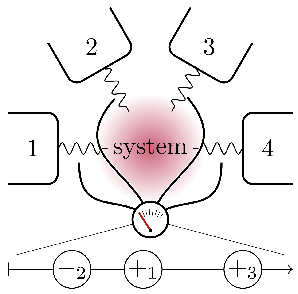
Figure 1: Exchanges between a system and reservoirs are monitored rather than the internal transitions of the system itself, yielding a trajectory that still carries thermodynamic information about the system. The squiggly arrows represent the monitored interactions that provide a trajectory comprised of multifilar events, represented as circles on a timeline.

More akin to statistical mechanics than to traditional thermodynamics, stochastic thermodynamics struggles when the said mesoscopic states are coarse-grained; for instance, there is no obvious path to EPR when measurements are not performed at the level of individual edges. Resolving individual edges and requiring visibility of all of them is a major setback for the application of stochastic thermodynamics to systems beyond toy models or specifically tailored experiments. Very recently, different methods have been explored to infer its value in a variety of scenarios, usually providing lower bounds. Some methods involve: an integral fluctuation theorem for hidden EPR due to variable separation Kawaguchi and Nakayama (2013); Herpich et al. (2020), thermodynamic uncertainty relations for current precision Manikandan et al. (2020); Busiello and Pigolotti (2019); Li et al. (2019); Van Vu et al. (2020), numerically solving an optimization problem Skinner and Dunkel (2021) or establishing masked dynamics Shiraishi and Sagawa (2015); Bisker et al. (2017); Ehrich (2021); Blom et al. (2023), which can involve quantifying asymmetries in forward and backward waiting-times distributions Roldán and Parrondo (2010); Martínez et al. (2019), time-scale separation Esposito (2012); Bo and Celani (2014); Rahav and Jarzynski (2007), the statistics of transitions when states are hidden Harunari et al. (2022); van der Meer et al. (2022, 2023); Harunari et al. (2023); Garilli et al. (2023), and others Maes (2017); Berezhkovskii and Makarov (2019); Cristadoro et al. (2023); Singh and Proesmans (2023); Ferri-Cortés et al. (2023); Liang and Pigolotti (2023); Ertel and Seifert (2023); Degünther et al. (2023); Yu et al. (2021); Baiesi et al. (2023); Hartich and Godec (2021); Lucente et al. (2023); Gnesotto et al. (2020); Lynn et al. (2022); Tan et al. (2021). See also a more detailed overview of recent approaches to nonequilibrium detection in Ref. Lucente et al. (2022).

Although the dynamics of mesoscopic systems is typically observed through changes in the environment, many of the mentioned methods fall short in this case since not necessarily a configuration change is uniquely associated with a change in the environment. As a paradigmatic example, consider a system in contact with many reservoirs that drive it away from equilibrium through the exchange of physical quantities; some examples are transport problems Walldorf et al. (2018); Landi (2021); Cuetara and Esposito (2015), photon detections Viisanen et al. (2015), Maxwell demons Sánchez et al. (2019); Freitas and Esposito (2021) and chemical reaction networks Rao and Esposito (2018a). Also, consider that the experimenter does not directly monitor the system, since it might be beyond the experimental limitations or too sensitive to perturbations. See Fig. 1 for an illustration. The measurements open the possibility of inferring system properties, such as the distance to equilibrium, but they pose additional challenges. Several distinct transitions between system mesostates usually give rise to the same event in a reservoir, and thus we dub them multifilar, rendering the trajectories non-Markovian. In this case, some of the previously known results do not apply, and the problem quickly becomes numerically expensive. Some other examples are a molecular motor with more than one configuration change leading to the observable step along a filament and a composite system that has two indistinguishable processes occurring at the same time.

In this contribution, we extend the framework for the statistics of a partial set of visible transitions Harunari et al. (2022); van der Meer et al. (2022) to the case of multifilar events and develop paths to detect and quantify nonequilibrium behavior in distinct scenarios using minimal assumptions. We start by formalizing the mathematical framework, obtaining analytical expressions for sequences of multifilar events and waiting-times based on first-passage problems, both in the semi-Markov approach and the fully non-Markovian case. We proceed by showing that the probabilities of each individual event compared to its time reverse bounds the EPR from below, this can be done with no prior knowledge of the system itself and can be applied to situations where the physical characteristics of the system and reservoirs are unknown or inaccessible. Second, we still do not require prior knowledge and turn to conditional probabilities, discussing a semi-Markov approach that is proven to not provide a lower bound; however, it forms a detector of nonequilibrium behavior from the event sequences and waiting-time distributions, and its estimation tends to be more feasible compared to higher-order approaches. Third, if prior knowledge of the system topology is present, which can come in the form of, e.g. possible chemical reactions or physical structure of a device, we put forward a simple method that measures the affinity and consequently provides the exact EPR bypassing the need for establishing a model and its transition rates. We describe scenarios to decide the suitability of each estimator and the conditions that hinder their relevance. The results are illustrated in relevant models, and we conclude by discussing the results and open questions.

II Framework for multifilar events

We consider a continuous-time Markov chain defined over an irreducible state space whose dynamics is captured by time-independent transition rates, establishing a master equation

$$d_{t}\mathbf{p}(t)=\mathbf{R}\mathbf{p}(t),$$ (1)

here $\mathbf{R}$ is the rate matrix with entries $R_{ij}$ being the transition rate from state $j$ to $i$ if $i\neq j$, or minus the exit rate $R_{ii}=-\sum_{j}R_{ji}$ otherwise. A pair of states $i\neq j$ can be connected by more than one transition, rendering the state space a multigraph, which can be expressed as

$$R_{ij}=\sum_{\ell}r_{\ell}\delta_{i,\mathsf{t}(\ell)}\delta_{j,\mathsf{s}(\ell)},$$ (2)

with the sum spanning over all transitions. In our notation, $\ell$ is a transition from source state $\mathsf{s}(\ell)$ to target state $\mathsf{t}(\ell)$, and its rate is rate $r_{\ell}$. The probability distribution will reach a unique stationary value at long times that will be, for simplicity, referred to as $\mathbf{p}$ since hereafter we assume stationarity.

From the set of all possible transitions between states, we consider that a subset $\mathcal{L}$ yields observable measurements. We assume “observable microreversibility”, the notion that all observable transitions $\ell\in\mathcal{L}$ can be performed in the opposite direction and produce an observable that can be distinguished from the original, i.e., $\bar{\ell}\in\mathcal{L}$ and $\ell\neq\bar{\ell}$. This ensures the thermodynamic consistency of observables.

A crucial step for this work is accounting for multifilar events: events that immediately emerge from the occurrence of more than one transition. As yet another example, consider a three-level system that exchanges matter with a lead; when an electron is transferred to the system, a jump can occur from the ground to the first excited state, or from the first to the second excited state, but the same increment is observed in the current system-lead in both cases. If energy exchanges are monitored, the multifilar character is present if the energy gaps between the three states are the same, otherwise it would be possible to distinguish the internal transitions. See Fig. 2.

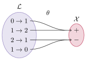
Figure 2: Example of multifilar events: Whenever a three-level system exchanges electrons with a metallic lead, a pair of transitions from space $\mathcal{L}$ is involved with a single event observed on the lead in $\mathcal{X}$. The map $\theta$ relating both is non-injective.

The relation between observable transitions and their respective multifilar events is given by the map $\theta:\mathcal{L}\to\mathcal{X}$, supported by the subset of all observable transitions. This map is non-injective; otherwise, it would not establish multifilar events. We also assume that each transition is associated with at most one multifilar event; otherwise, $\theta$ would not be a map. Since the reverse of an observable transition is also observable, the reverse of an element $x\in\mathcal{X}$ is also a multifilar event $\bar{x}\in\mathcal{X}$. As should, the coarse-graining map commutes with time reversal: $\theta\bar{\ell}=\bar{x}$ for $\theta\ell=x$. If the timeseries of observable transitions is

$$\ell_{0}\xrightarrow{t_{1}}\ell_{1}\xrightarrow{t_{2}}\cdots\xrightarrow{t_{n}}\ell_{n},$$ (3)

then the observation of multifilar events yields

$$\theta\ell_{0}\xrightarrow{t_{1}}\theta\ell_{1}\xrightarrow{t_{2}}\cdots\xrightarrow{t_{n}}\theta\ell_{n}.$$ (4)

In principle, a multifilar event is a label given to one or more observable transitions produced by the Markov process.

II.1 Semi-Markov

Even though the sequence of events is non-Markovian, a semi-Markov treatment is relevant for practical purposes. Empirical estimation of the statistics of more than two events often becomes computationally challenging or requires the acquisition of a lot of data. For this reason, we start exploring the statistics between a pair of events, which can be later used to probe collected data or to evaluate quantities under the semi-Markov assumption.

Immediately after a multifilar event $x$, the probability distribution in the state space is a statistical mixture of all possible targets of transitions in the subset $\theta^{-1}x\subset\mathcal{L}$. The non-delta distribution after an event breaks the renewal property, introducing non-Markovianity in the sequence of multifilar events. By comparing the rates at which transitions occur, this distribution can be expressed as

$$\mathbf{p}_{|x}=\bm{\Gamma}_{x}\mathbf{p},$$ (5)

where we define the event-propagating matrix

$$\bm{\Gamma}_{x}\coloneqq\frac{1}{\mathcal{K}_{x}}\sum_{\ell\in\theta^{-1}x}r_{\ell}\bm{\Delta}_{\ell}.$$ (6)

We also define $\bm{\Delta}_{\ell}$ as a square matrix of size equals to the cardinality of the state space and whose elements are zeros but for 1 in the element of row $\mathsf{t}(\ell)$ and column $\mathsf{s}(\ell)$ , and $\mathcal{K}_{x}\coloneqq\sum_{\ell\in\theta^{-1}x}r_{\ell}p_{\mathsf{s}(\ell)}$ as the traffic rate of event $x$ (also known as its dynamical activity, a time-symmetric observable). The observable traffic rate, which measures the number of all events per unit time, is then $\mathcal{K}\coloneqq\sum_{x}\mathcal{K}_{x}$.

The state space propagation between two observable multifilar events can be obtained by solving a first-passage problem in an auxiliary dynamics Harunari et al. (2022); Sekimoto (2021). Let $\mathbf{S}\coloneqq\mathbf{R}-\sum_{\ell\in\mathcal{L}}r_{\ell}\bm{\Delta}_{\ell}$ be the survival propagator, then $\exp(t\mathbf{S})$ propagates the probability distribution for a duration $t$ conditioned on the absence of observable transitions and $r_{\ell}[\exp(t\mathbf{S})\mathbf{p}]_{\mathsf{s}(\ell)}$ is the probability of performing transition $\ell$ after time $t$ starting from any $\mathbf{p}$. The survival matrix can also be expressed in terms of Eq. (6):

$$\mathbf{S}=\mathbf{R}-\sum_{x\in\mathcal{X}}\mathcal{K}_{x}\bm{\Gamma}_{x}.$$ (7)

At the level of observable transitions, we can now obtain the probability of transition $\ell$ occurring after time $t$ has passed since the multifilar event $x$,

$$P(\ell,t|x)=r_{\ell}\left[e^{t\mathbf{S}}\bm{\Gamma}_{x}\mathbf{p}\right]_{\mathsf{s}(\ell)}.$$ (8)

Finally, the probability of another event occurring after time $t$ can be obtained by another usage of the matrix $\bm{\Gamma}$,

$$P(x\raise 1.72218pt\hbox{$\scriptstyle\prime$},t|x)=\mathcal{K}_{x\raise 1.20552pt\hbox{$\scriptstyle\prime$}}\bm{1}\bm{\Gamma}_{x\raise 1.20552pt\hbox{$\scriptstyle\prime$}}e^{t\mathbf{S}}\bm{\Gamma}_{x}\mathbf{p},$$ (9)

with $\bm{1}$ being a row vector of ones. See App. A for a proof.

As proven in Harunari et al. (2023) and with an alternative approach in App. B, the survival matrix is invertible. Therefore, marginalizing the waiting-time leads to the probability of one event $x\raise 1.72218pt\hbox{$\scriptstyle\prime$}$ conditioned on the previous event $x$:

$$P(x\raise 1.72218pt\hbox{$\scriptstyle\prime$}|x)=-\mathcal{K}_{x\raise 1.20552pt\hbox{$\scriptstyle\prime$}}\bm{1}\bm{\Gamma}_{x\raise 1.20552pt\hbox{$\scriptstyle\prime$}}\mathbf{S}^{-1}\bm{\Gamma}_{x}\mathbf{p}.$$ (10)

Although this equation is only conditioned on the last multifilar event $x$, it does not mean the process is Markovian. The probability of a long sequence of events cannot be expressed by the multiplication of probabilities similar to Eq. (10).

Equations (9) and (10) represent the statistics of pairs of multifilar events that will be used for thermodynamic inference in the following sections. They can be empirically estimated from experiments or numerical simulations. The transition-based coarse-graining framework is recovered from these equations by choosing an injective map $\theta$. In this case, all matrices $\Gamma$ are single-entry, $\mathbf{p}_{x}$ has only a single entry 1, and the renewal property is recovered, leading to Markovian sequences of observable transitions.

II.2 Non-Markov

The more general non-Markovian probability of a sequence of multifilar events can also be estimated using the introduced tools. The sequence of transitions and intertransition times, which is Markovian, is obtained by the path probability

$$P\left(\vec{\ell},\vec{t}\,\right)=P(\ell_{0})\prod_{i=1}^{n}P(\ell_{i},t_{i}|\ell_{i-1}),$$ (11)

for $\vec{\ell}=\{\ell_{0},\ldots,\ell_{n}\}$ and $\vec{t}=\{t_{1},\ldots,t_{n}\}$. An expression analogous to Eq. (11) for $\vec{x}$ would represent the semi-Markov approximation. The path probability of multifilar events can be obtained from all possible sequences of observable transitions that map onto the sequence of events, i.e.,

$$P\left(\vec{x},\vec{t}\,\right)=\sum_{\vec{\ell}\in\mathcal{L}^{n+1}}P\left(\vec{\ell},\vec{t}\,\right)\prod_{i=0}^{n}\delta_{\theta\ell_{i},x_{i}},$$ (12)

where $\delta$ is the Kronecker delta function.

Using the event-propagating matrix $\bm{\Gamma}_{x}$ defined in Eq. (6), this probability can be obtained by

$$P\left(\vec{x},\vec{t}\,|x_{0}\right)=\left(\prod_{i=1}^{n}\mathcal{K}_{x_{i}}\right)\mathbf{1}\left(\prod_{i=n}^{1}\bm{\Gamma}_{x_{i}}e^{t_{i}\mathbf{S}}\right)\bm{\Gamma}_{x_{0}}\mathbf{p},$$ (13)

where the product $\prod_{i=n}^{1}$ is ordered with larger $i$ on the left, i.e., $\bm{\Gamma}_{x_{n}}\exp(t_{n}\mathbf{S})\bm{\Gamma}_{x_{n-1}}\exp(t_{n-1}\mathbf{S})\cdots$. This equation provides the joint probability density of a non-Markovian sequence of events $\vec{x}$ and their waiting-times $\vec{t}$. As in the previous case, this probability can be marginalized by integration of all waiting-times and the matrix exponentials will be replaced by $-\mathbf{S}^{-1}$.

Equation (13) captures the path probability of each individual sequence of transitions that is compatible with the considered sequence of events. Intuitively, $\exp(t\mathbf{S})$ captures the propagation through hidden pathways interspersed by multifilar events captured by $\mathbf{\Gamma}$.

Loosely speaking, the multiplication by $\mathbf{1}$ from the left, or taking the trace, pinpoints the level of Markovianity assumed. Multiplying several values of Eq. (9) to form the semi-Markov probability of a larger sequence will display $\mathbf{1}$ at every two matrices $\bm{\Gamma}$.

III Detecting and quantifying nonequilibrium

The EPR of a continuous-time Markov chain is

$$\sigma=\sum_{ij}R_{ji}p_{i}\ln\frac{R_{ji}p_{i}}{R_{ij}p_{j}}$$ (14)

in units of the Boltzmann constant Schnakenberg (1976). The quantities involved are transition rates and probability mass functions, and measuring EPR requires a method for their inference. Establishing a model involves the definition of the possible states and the transition rates between them, thus solving the master equation yields the probabilities and EPR is obtained. If no model is available, but all states can be observed, transition rates can be empirically obtained by the frequencies of each transition and probabilities are obtained from residence times. If there is a model but missing information, such as some inaccessible transition rates due to hidden states, many of the methods mentioned in Sec. I can be used to estimate the EPR. Alternatively, it is also possible to devise model-free estimators that make no assumptions regarding the topology, existence of hidden states and their number, values of some transition rates, or more. These model-free estimators are invaluable for applying nonequilibrium thermodynamic methods to assess energetic interchanges, physical limitations, and the arrow of time in natural systems. When a model-free estimator is employed, its result is not conditioned on the validity of model assumptions. In the context of observing multifilar events, we discuss two model-free estimators and one that uses topological information to assess the distance to equilibrium.

In this section, we will assume that all transitions of the system are visible through multifilar events, i.e., $\mathcal{L}$ is the complete set of transitions of the Markov process. For each case, we will discuss the implications of hidden transitions, without loss of generality, by assuming that their associated event is itself hidden a posteriori.

III.1 Zero-knowledge

The first model-free estimator considers the (unconditioned) probability of each event,

$$P(x)=\sum_{\ell\in\theta^{-1}x}P(\ell)=\sum_{\ell\in\theta^{-1}x}\frac{r_{\ell}p_{\mathrm{s}(\ell)}}{\mathcal{K}},$$ (15)

which can also be empirically obtained from frequencies. With no requirements beyond the already announced assumptions, the log-sum inequality applied to Eq. (14) establishes the lower bound

$$\sigma_{\text{zk}}\coloneqq\mathcal{K}\sum_{x\in\mathcal{X}}P(x)\ln\frac{P(x)}{P(\bar{x})}\leq\sigma.$$ (16)

If the multifilar events are associated with currents, it can be convenient to define $j_{x}\coloneqq\mathcal{K}[P(x)-P(\bar{x})]$ and

$$\sigma_{\text{zk}}=\frac{1}{2}\sum_{x\in\mathcal{X}}j_{x}\ln\frac{P(x)}{P(\bar{x})},$$ (17)

where $\ln P(x)/P(\bar{x})$ acts as the effective affinity of each multifilar event.

Recall that the value of $\mathcal{K}$ is context-dependent, it is the traffic rate of all visible multifilar events. Therefore, it can always be measured by counting their number and dividing by the time span. The occurrence of hidden transitions does not contribute to its value.

With the estimator in Eq. (16), it is possible to bound the EPR from below using the statistics of each event in the absence of any knowledge about the exchanged quantities, the system topology, or physical characteristics such as the chemical potentials or temperatures of reservoirs. As will be illustrated, the bound can be tight even in the presence of $\theta^{-1}x$ with infinite cardinality, as in chemical reaction networks.

Each individual term in Eq. (16) is non-negative and thus it still constitutes a lower bound if some events are hidden.

III.2 Waiting-times

When all transitions in a process are visible and distinguishable, waiting-time distributions generally do not play a role in entropy production Harunari et al. (2022); van der Meer et al. (2022), since all are Poisson distributions of respective exit rates. The same is not valid for events due to their multifilar nature; thus, waiting-time distributions can entail additional thermodynamic information. Therefore, a very natural extension lies in considering the statistics of pairs of transitions, in which a semi-Markov approximation would be performed on the non-Markovian trajectories of events. Since it constitutes an approximation, the expressions can overestimate the real EPR, which is fundamentally a problem when the goal is to estimate thermodynamic costs and limits of a given process. Similarly, it has recently been suggested that waiting-times have to be disregarded in the semi-Markov approach Blom et al. (2023). Also, if a condition known as “transition-preserving” Ertel and Seifert (2023) is satisfied, both the sequence of events (referred to as blurred transitions in Ref. Ertel and Seifert (2023)) and their waiting-times constitute a lower bound for the EPR. However, in the present work we do not explore this direction since it requires some knowledge of the internal topology that we assume is not available.

If all system transitions $\mathcal{L}$ are distinguishable, the expression in Ref. Harunari et al. (2022) for the EPR in the transition-based framework is

$$\sigma=\mathcal{K}\sum_{\ell^{\prime},\ell\in\mathcal{L}}\int_{0}^{\infty}\mathrm{d}tP(\ell,\ell^{\prime},t)\ln\frac{P(\ell^{\prime},t|\ell)}{P(\overline{\ell},t|\overline{\ell^{\prime}})},$$ (18)

where $P(\ell,\ell^{\prime},t)$ is the joint probability density function for the occurrence of two consecutive transitions $\ell$ and $\ell^{\prime}$ separated by a time interval $t$. If the log-sum inequality is applied to make sums of multifilar events pop out, the result is

$$\sigma \geq\mathcal{K}\sum_{x,x\raise 1.20552pt\hbox{$\scriptstyle\prime$}\in\mathcal{X}}\int_{0}^{\infty}\mathrm{d}tP(x,x\raise 1.72218pt\hbox{$\scriptstyle\prime$},t)\ln\frac{P(x\raise 1.72218pt\hbox{$\scriptstyle\prime$},t|x)}{P(\overline{x},t|\overline{x\raise 1.72218pt\hbox{$\scriptstyle\prime$}})}$$

$$\phantom{\geq\ }+\mathcal{K}\sum_{x\in\mathcal{X}}P(x)\ln\frac{P(x)}{P(\overline{x})}-\mathcal{K}\sum_{\ell\in\mathcal{L}}P(\ell)\ln\frac{P(\ell)}{P(\overline{\ell})},$$ (19)

where the first term is $\expectationvalue{\hat{\sigma}_{\text{BT}}}$ from Ref. Ertel and Seifert (2023), the second is the entropy difference between forward and backward statistics of events, while the last is the same but for transitions. The sum of the last two is nonpositive, thus the first term cannot form a lower bound, at least in the general case. More specifically, the last term itself is also nonpositive, which otherwise would be very useful since it is the only one that depends on the internal details of the system, beyond multifilar events.

In equilibrium, the first term of Eq. (III.2) vanishes. Notice that, since all transitions are observed–even if indistinguishably–the survival matrix $\mathbf{S}$ is diagonal with entries equivalent to minus exit rates $\mathrm{exit}(\bullet)\coloneqq-R_{\bullet,\bullet}$. Therefore,

$$P(\ell,\ell^{\prime},t)=r_{\ell^{\prime}}\exp\{t\,\mathrm{exit}(\mathsf{s}(\ell^{\prime}))\}\frac{r_{\ell}p_{\mathsf{s}(\ell)}}{\mathcal{K}}\delta_{\mathsf{s}(\ell^{\prime}),\mathsf{t}(\ell)}.$$ (20)

Also, since equilibrium is considered, the detailed balance condition, $r_{\ell}p_{\mathrm{s}(\ell)}^{\text{eq}}=r_{\overline{\ell}}p_{\mathrm{s}(\overline{\ell})}^{\text{eq}}$ ensures

$$P_{\text{eq}}(\ell,\ell^{\prime},t)=P_{\text{eq}}(\overline{\ell^{\prime}},\overline{\ell},t),$$ (21)

where we used $\mathrm{s}(\ell^{\prime})=\mathrm{t}(\ell)=\mathrm{s}(\overline{\ell})$, which we stress is valid under the assumption that all transitions are observable. Marginalizing the waiting-times provides $P_{\text{eq}}(\ell,\ell^{\prime})=P_{\text{eq}}(\overline{\ell^{\prime}},\overline{\ell})$.

Back to multifilar events $x\in\mathcal{X}$, we can sum the results above and obtain

$$P_{\text{eq}}(x,x\raise 1.72218pt\hbox{$\scriptstyle\prime$})=P_{\text{eq}}(\overline{x\raise 1.72218pt\hbox{$\scriptstyle\prime$}},\overline{x}),$$ (22)

$$P_{\text{eq}}(t|x,x\raise 1.72218pt\hbox{$\scriptstyle\prime$})=P_{\text{eq}}(t|\overline{x\raise 1.72218pt\hbox{$\scriptstyle\prime$}},\overline{x\raise 1.72218pt\hbox{$\scriptstyle\prime$}}),$$ (23)

which shows that the sequences of events and their waiting-times are symmetric under time-reversal when at equilibrium, as expected.

Although the sum of the first and second terms of Eq. (III.2), the event-exclusive terms, does not establish a lower bound for the EPR in general, it vanishes at equilibrium and is nonnegative. This sum can be split into two terms,

$$D_{x}\coloneqq\sum_{x,x\raise 1.20552pt\hbox{$\scriptstyle\prime$}\in\mathcal{X}}P(x,x\raise 1.72218pt\hbox{$\scriptstyle\prime$})\ln\frac{P(x,x\raise 1.72218pt\hbox{$\scriptstyle\prime$})}{P(\overline{x\raise 1.72218pt\hbox{$\scriptstyle\prime$}},\overline{x})}$$ (24)

and

$$D_{t}\coloneqq\sum_{x,x\raise 1.20552pt\hbox{$\scriptstyle\prime$}\in\mathcal{X}}P(x,x\raise 1.72218pt\hbox{$\scriptstyle\prime$})D_{\text{KL}}[P(t|x,x\raise 1.72218pt\hbox{$\scriptstyle\prime$})||P(t|\overline{x\raise 1.72218pt\hbox{$\scriptstyle\prime$}},\overline{x})],$$ (25)

where we denote as $D_{\text{KL}}[P(t)||Q(t)]$ the Kullback-Leibler divergence for continuous variables (see  for practical considerations) between $P(t)$ and $Q(t)$, which is the relative entropy of both distributions, and vanishes if and only if the distributions are the same. Equations (24) and (25) are relative entropies between a pair of events and its time-reversal, the former accounts for pairs of multifilar events and the latter for their waiting-times. Both are nonnegative and vanish at equilibrium, satisfying minimal conditions to be used as indicators of nonequilibrium behavior.

Importantly, the values of Eq. (24) and (25) are nonnegative for any choice of $\mathcal{X}$, and therefore are nonequilibrium detectors even if some events are hidden or there exist transitions not associated with events. Once again, we recall that if $x\in\mathcal{X}$ then $\bar{x}\in\mathcal{X}$. In summary, a positive value of $D_{x}$ or $D_{t}$ for any set of visible multifilar events $\mathcal{X}$ is enough evidence for an underlying nonequilibrium process.

The irreversibility in $D_{x}$ and $D_{t}$ is captured by comparing statistics and waiting-times of a pair of events and its time reversal. If the only observables are one event and its reverse, $\mathcal{X}=\{x,\bar{x}\}$, irreversibility can be detected by comparing $(x,x)$ and $(\bar{x},\bar{x})$, while the contribution from alternated terms $(x,\bar{x})$ and $(\bar{x},x)$ vanish. Therefore, even if $P(x)=P(\bar{x})$, which represents apparent equilibrium due to a stalled observable current, irreversibility can still be detected.

III.3 Topology-informed

Additional information opens the possibility of analyzing the event statistics through a more informed lens and obtaining better bounds or estimators. We consider the case of knowledge about the state space topology, which is generally not enough to measure the EPR since it requires dynamical information in the form of transition rates.

A few classes of systems present a particular symmetry in the state space: more than one cycle with the same affinity, potentially an infinite number of them. In these cases, usually, the same sequence of observables occurs each time one of such cycles is performed. In chemical reactions, this usually happens because the affinity might depend only on the propensities and chemostatted concentrations, thus being independent of local configurations. In systems satisfying local detailed balance (LDB), which is a condition for thermodynamic consistency Esposito (2012); Falasco and Esposito (2021), the affinity reduces to a sum over the entropy fluxes generated by each transition along the cycle. The result of this sum usually involves physical properties such as temperatures, energy exchanges, and chemical potentials, but not local state probabilities , and can result in the same value for families of cycles since conserved quantities cancel Polettini et al. (2016); Rao and Esposito (2018b). Notice that these are common mechanisms giving rise to said symmetry, but not necessary conditions.

For the next estimator, we assume the following: There exists a finite number of families of cycles of the same affinity and, for each family, there is a unique minimal sequence of events $\vec{x}_{\alpha}$ univocally defining the completion of a cycle $\vec{\mathcal{C}}_{\alpha}$ from this family [see Section V for examples].

Network theory Schnakenberg (1976); Avanzini et al. (2023) says that the affinity of a cycle is given by the product of the rates of all edges involved, according to their convention orientation,

$$A_{\alpha}=\ln\frac{\prod_{\ell\in\vec{\mathcal{C}}_{\alpha}}r_{\ell}}{\prod_{\ell\in{\mathchoice{\vbox{\offinterlineskip\halign{#\cr\reflectbox{$\displaystyle\vec{}\mkern 4.0mu$}\cr\kern-3.01389pt\cr$\displaystyle\mathcal{C}$\cr}}}{\vbox{\offinterlineskip\halign{#\cr\reflectbox{$\textstyle\vec{}\mkern 4.0mu$}\cr\kern-3.01389pt\cr$\textstyle\mathcal{C}$\cr}}}{\vbox{\offinterlineskip\halign{#\cr\reflectbox{$\scriptstyle\vec{}\mkern 4.0mu$}\cr\kern-2.10971pt\cr$\scriptstyle\mathcal{C}$\cr}}}{\vbox{\offinterlineskip\halign{#\cr\reflectbox{$\scriptscriptstyle\vec{}\mkern 4.0mu$}\cr\kern-1.50694pt\cr$\scriptscriptstyle\mathcal{C}$\cr}}}}_{\alpha}}r_{\ell}}.$$ (26)

Next, we turn to the probability of observing a sequence $\vec{x}_{\alpha}$. It is given by the sum of probabilities of all transition sequences associated with $\vec{x}_{\alpha}$:

$$P(\vec{x}_{\alpha})=\sum_{\vec{\ell}:\theta\vec{\ell}=\vec{x}_{\alpha}}P(\vec{\ell}\,)=\sum\frac{r_{\ell_{0}}p_{\mathsf{s}(\ell_{0})}}{\mathcal{K}}\prod_{i}\frac{r_{\ell_{i}}}{\mathrm{exit}(\mathsf{s}(\ell_{i}))},$$ (27)

which can be obtained from Eq. (13). Since we assumed a one-to-one connection between a family of same-affinity cycles $\vec{\mathcal{C}}_{\alpha}$ and a sequence of transitions $\vec{x}_{\alpha}$, Eq. (26) can be plugged in the right-hand side of Eq. (27), making the factor $\exp(A_{\alpha})$ appear, and the log-ratio with the time-reversed sequence simplifies to

$$\ln\frac{P(\vec{x}_{\alpha})}{P({\mathchoice{\vbox{\offinterlineskip\halign{#\cr\reflectbox{$\displaystyle\vec{}\mkern 4.0mu$}\cr\kern-4.30554pt\cr$\displaystyle x$\cr}}}{\vbox{\offinterlineskip\halign{#\cr\reflectbox{$\textstyle\vec{}\mkern 4.0mu$}\cr\kern-4.30554pt\cr$\textstyle x$\cr}}}{\vbox{\offinterlineskip\halign{#\cr\reflectbox{$\scriptstyle\vec{}\mkern 4.0mu$}\cr\kern-3.01389pt\cr$\scriptstyle x$\cr}}}{\vbox{\offinterlineskip\halign{#\cr\reflectbox{$\scriptscriptstyle\vec{}\mkern 4.0mu$}\cr\kern-2.15277pt\cr$\scriptscriptstyle x$\cr}}}}_{\alpha})}=A_{\alpha}.$$ (28)

${\mathchoice{\vbox{\offinterlineskip\halign{#\cr\reflectbox{$\displaystyle\vec{}\mkern 4.0mu$}\cr\kern-4.30554pt\cr$\displaystyle x$\cr}}}{\vbox{\offinterlineskip\halign{#\cr\reflectbox{$\textstyle\vec{}\mkern 4.0mu$}\cr\kern-4.30554pt\cr$\textstyle x$\cr}}}{\vbox{\offinterlineskip\halign{#\cr\reflectbox{$\scriptstyle\vec{}\mkern 4.0mu$}\cr\kern-3.01389pt\cr$\scriptstyle x$\cr}}}{\vbox{\offinterlineskip\halign{#\cr\reflectbox{$\scriptscriptstyle\vec{}\mkern 4.0mu$}\cr\kern-2.15277pt\cr$\scriptscriptstyle x$\cr}}}}_{\alpha}$ is defined as the time-reversal of the original sequence and can be obtained by reversing the order of the sequence and the direction of each individual event: $x\leftrightarrow\overline{x}$. This time-reversal is nothing but the result of coarse-graining the time-reversed state space trajectory. For clarity, if $\vec{x}_{\alpha}=\{x_{0},\ldots,x_{n}\}$, then ${\mathchoice{\vbox{\offinterlineskip\halign{#\cr\reflectbox{$\displaystyle\vec{}\mkern 4.0mu$}\cr\kern-4.30554pt\cr$\displaystyle x$\cr}}}{\vbox{\offinterlineskip\halign{#\cr\reflectbox{$\textstyle\vec{}\mkern 4.0mu$}\cr\kern-4.30554pt\cr$\textstyle x$\cr}}}{\vbox{\offinterlineskip\halign{#\cr\reflectbox{$\scriptstyle\vec{}\mkern 4.0mu$}\cr\kern-3.01389pt\cr$\scriptstyle x$\cr}}}{\vbox{\offinterlineskip\halign{#\cr\reflectbox{$\scriptscriptstyle\vec{}\mkern 4.0mu$}\cr\kern-2.15277pt\cr$\scriptscriptstyle x$\cr}}}}_{\alpha}=\{\bar{x}_{n},\ldots,\bar{x}_{0}\}$.

Having estimated affinities, it is a matter of finding the cycle currents $j_{\alpha}$. Depending on the model, they can be obtained from reservoir fluxes or by the flux over chords (edges removed from the network to define a spanning tree that forms the cycle in question when reintroduced). Given that the topology is known, defining this flux is most likely immediate. Bringing all together, we have the topology-informed estimator

$$\sigma_{\text{ti}}\coloneqq\sum_{\alpha}j_{\alpha}\ln\frac{P(\vec{x}_{\alpha})}{P({\mathchoice{\vbox{\offinterlineskip\halign{#\cr\reflectbox{$\displaystyle\vec{}\mkern 4.0mu$}\cr\kern-4.30554pt\cr$\displaystyle x$\cr}}}{\vbox{\offinterlineskip\halign{#\cr\reflectbox{$\textstyle\vec{}\mkern 4.0mu$}\cr\kern-4.30554pt\cr$\textstyle x$\cr}}}{\vbox{\offinterlineskip\halign{#\cr\reflectbox{$\scriptstyle\vec{}\mkern 4.0mu$}\cr\kern-3.01389pt\cr$\scriptstyle x$\cr}}}{\vbox{\offinterlineskip\halign{#\cr\reflectbox{$\scriptscriptstyle\vec{}\mkern 4.0mu$}\cr\kern-2.15277pt\cr$\scriptscriptstyle x$\cr}}}}_{\alpha})}=\sigma,$$ (29)

which is exactly the EPR. It is important to note that there exists some freedom in the definition of cycles, hence if the family of cycles that meet the requirements is not known, the following recipe can be followed for systems with finite state space: (i) choose a spanning tree (cf. Schnakenberg (1976)), (ii) identify cycles that share the same affinity and can be univocally defined by a sequence $\vec{x}_{\alpha}$, (iii) measure the current at the chords of these cycles and the affinity using Eq. (28). The method does not necessarily satisfy the assumption for every choice of spanning tree, so it might need to be repeated. For infinite state spaces, such as the concentration space of chemical reaction networks, the definition of a same-affinity cycle family usually comes from the list of reactions and chemostatted species.

We recall that the sequence of multifilar events is non-Markovian, the probabilities $P(\vec{x}_{\alpha})$ can be empirically obtained or calculated by the path probability of events, Eq. (13). However, if a semi-Markov approximation is performed, the estimator can be employed to obtain an approximated value of the EPR that might be more feasible, since assessing the statistics of long sequences often becomes challenging.

For the topology-informed estimator $\sigma_{\text{ti}}$, a partial sum of Eq. (29) will not lead to an EPR lower bound since some terms might be negative, which is usually the case in heat engines, for example. Therefore, all families of cycles must be considered. However, it is possible that the assumption of $\sigma_{\text{ti}}$ still holds in the presence of hidden transitions since some might belong to zero-affinity cycles or to cycles that do not contribute to the EPR due to conservation laws. In other words, hidden transitions do not immediately rule out the assumption herein.

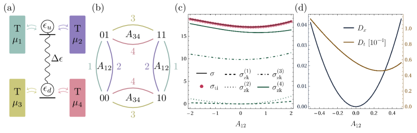
Figure 3: (a) Scheme of the double quantum-dot with four reservoirs and Coulomb repulsion; (b) state space with degenerate affinities $A_{12}$ and $A_{34}$ and the label/color of each edge represents the reservoir mediating the transitions and, therefore, its associated multifilar event observed from the reservoirs; (c) In terms of affinity $A_{12}$, EPR, topology-informed estimator, and zero-knowledge estimators for the observation of 1, 2, 3 and all reservoirs. (d) Nonequilibrium detectors evaluated with the statistics of reservoir 1. More details in the main text.

IV The case of reservoirs: a cautionary tale

A quintessential problem in nonequilibrium thermodynamics consists of a system placed in contact with more than one reservoir with which it can exchange energy and/or matter. This is used to model electronic devices between leads, quantum transport problems, chemostatted chemical reactions, and the historical problem of a heat engine working between a hot and a cold reservoir. The events occurring at the reservoirs are usually multifilar and can be used to obtain entropy production through integrated currents if the physical quantities of all reservoirs are known. Let $\mathbf{F}$ denote the fundamental forces, a set of nonconservative forces obtained by combining the physical properties of reservoirs and conservation laws Polettini et al. (2016); Rao and Esposito (2018b), the EPR is

$$\sigma=\mathbf{j}\cdot\mathbf{F}$$ (30)

in the long-time limit and in units of the Boltzmann constant, where $\mathbf{j}$ are physical currents associated with each force. Therefore, if fundamental forces are known, it is only required to measure values of currents, ruling out the need for inference schemes that employ, e.g. waiting-times analysis or semi-Markov approximations. It is worth pointing out that conservation laws might render some reservoirs futile, thus the number of fundamental forces can be smaller than the number of reservoirs, and the currents from futile reservoirs need not be monitored.

Fundamental forces are composed of quantities such as temperature, energy gaps, charges, and chemical potentials, but they may not be known or measurable with the desired accuracy. In these situations, specialized estimators provide tools to assess EPR or the presence of nonequilibrium behavior. The inverse problem is also relevant; once the EPR is estimated and the currents are known, something can be said about the fundamental forces. Now, we discuss how the results of previous sections can contribute to the case of observing events in reservoirs without knowing the thermodynamic forces.

In the case of reservoirs, the multifilar events are often increments $\pm 1$ of a counter that monitors the number of exchanged quantities. If energy exchanges can be monitored and sufficiently resolved, it might be possible to monitor individual transitions or increase the space of multifilar events, improving the estimations. Without loss of generality, we assume that all transitions between states are mediated by reservoirs. If some transitions are hidden, we imagine an extra reservoir mediating all of these transitions, so this scenario is always covered by the case of hidden reservoirs. The quantities $\sigma_{\text{zk}}$, $D_{x}$ and $D_{t}$ are obtained as a sum of nonnegative terms, hence they can be used even when some reservoirs are hidden. Their values increase with the number of monitored reservoirs, thus the bound due to $\sigma_{\text{zk}}$ gets tighter, and it becomes increasingly easier to determine that $D_{x}$ or $D_{t}$ are nonzero from finite data. Lastly, the estimator $\sigma_{\text{ti}}$ requires visibility of all the reservoirs involved in the completion of cycles $\vec{\mathcal{C}}_{\alpha}$, which does not necessarily include all reservoirs.

The relation between fundamental forces and affinities, if the local detailed balance condition is satisfied, is given by a “$M$-matrix” Polettini et al. (2016) that captures the state space topology and the physical exchanges with each reservoir along all transitions. In some problems, it might be possible to relate the independent left-null vectors of this matrix and establish a direct connection between the affinity estimator in Eq. (28) and fundamental forces. However, we recall that, if the $M$-matrix is known, it is possible to obtain forces and currents analytically.

V Illustrations

V.1 Double quantum-dot

Motivated by Borrelli et al. (2015); Cuetara and Esposito (2015); Freitas and Esposito (2021), we consider a model for two quantum-dots (two-level systems), each coupled to two reservoirs, whose interaction occurs by Coulomb repulsion. See Fig. 3(a) for the model scheme. We assume that all four reservoirs have the same temperature $T=\beta^{-1}$ but different chemical potentials $\mu_{\nu}$, the quantum-dots when occupied have energies $\epsilon_{\text{u}}$ and $\epsilon_{\text{d}}$, and the interaction between occupied dots carries energy $\Delta\epsilon$. Transition rates satisfy LDB and thus the same affinity is present in distinct cycles as in Fig. 3(b).

If $\mu_{1}\neq\mu_{2}$ and $\mu_{3}\neq\mu_{4}$, the system is out of equilibrium and currents are established between each pair of reservoirs, passing through the quantum-dot between them. If $\Delta\epsilon\neq 0$, both quantum-dots interact, and the currents are the result of every parameter of the system. Let $\nu$ be the index representing each reservoir, we consider transition rates for $\nu=\{1,2\}$

$$R_{01,00}^{(\nu)} =\Gamma_{\nu}f(\epsilon_{\text{u}}-\mu_{\nu}),$$

$$R_{00,01}^{(\nu)} =\Gamma_{\nu}[1-f(\epsilon_{\text{u}}-\mu_{\nu})],$$

$$R_{11,10}^{(\nu)} =\Gamma_{\nu}f(\epsilon_{\text{u}}+\Delta\epsilon-\mu_{\nu}),$$

$$R_{10,11}^{(\nu)} =\Gamma_{\nu}[1-f(\epsilon_{\text{u}}+\Delta\epsilon-\mu_{\nu})],$$ (31)

where $\Gamma_{\nu}$ is the coupling strength to the reservoir and $f(\epsilon)=[1+\exp(\beta\epsilon)]^{-1}$ is the Fermi-Dirac distribution. For $\nu=\{3,4\}$ they are

$$R_{10,00}^{(\nu)} =\Gamma_{\nu}f(\epsilon_{\text{d}}-\mu_{\nu}),$$

$$R_{00,10}^{(\nu)} =\Gamma_{\nu}[1-f(\epsilon_{\text{d}}-\mu_{\nu})],$$

$$R_{11,01}^{(\nu)} =\Gamma_{\nu}f(\epsilon_{\text{d}}+\Delta\epsilon-\mu_{\nu}),$$

$$R_{01,11}^{(\nu)} =\Gamma_{\nu}[1-f(\epsilon_{\text{d}}+\Delta\epsilon-\mu_{\nu})].$$ (32)

In the plots of Fig. 3, their values are: $\{\Gamma_{1},\Gamma_{2},\Gamma_{3},\Gamma_{4}\}=\{11,5,7,13\}$, $\{\mu_{1},\mu_{3},\mu_{4}\}=\{5,6,1\}$, $\mu_{2}$ takes values in $[3,7]$ in panel (c) and $[4.5,5.5]$ in (d), $\beta=1$ and $\{\epsilon_{\text{u}},\epsilon_{\text{d}},\Delta\epsilon\}=\{2,1,3\}$.

The state space presents five cycles, and two pairs share the same affinity due to LDB and isothermality. An analysis of the fundamental forces Polettini et al. (2016); Rao and Esposito (2018b) reveals that only two affinities contribute to the EPR:

$$\sigma=\beta(\mu_{1}-\mu_{2})J_{1}+\beta(\mu_{3}-\mu_{4})J_{3}=A_{12}J_{1}+A_{34}J_{2},$$ (33)

where $J_{1}\coloneqq R_{01,00}^{(1)}p_{00}-R_{00,01}^{(1)}p_{01}+R_{11,10}^{(1)}p_{10}-R_{10,11}^{(1)}p_{11}$ is the flux from reservoir 1 t the system, and $J_{3}\coloneqq R_{10,00}^{(3)}p_{00}-R_{00,10}^{(3)}p_{10}+R_{11,01}^{(3)}p_{01}-R_{01,11}^{(3)}p_{11}$.

We consider electrons hopping into each reservoir as the observable multifilar events, which can be caused by distinct transitions and detected as increments in the voltage or a monitored current. For example, when a particle is provided by the first reservoir, we observe $+_{1}$, and it can be similarly associated to either $00\xrightarrow{1}01$ or $10\xrightarrow{1}11$.

For the estimator $\sigma_{\text{zk}}$, we do not need to use any of the above analyses, as it is a model-free estimator. Its values are shown in Fig. 3(c) for four cases, representing different amounts of information collected at the reservoirs. $\sigma_{\text{zk}}^{(1)}$ stands for the observation of reservoir 1, $\sigma_{\text{zk}}^{(2)}$ for reservoirs 1 and 2, $\sigma_{\text{zk}}^{(3)}$ for 1 to 3, and $\sigma_{\text{zk}}^{(4)}$ for all reservoirs. As expected, the bound tightens with the number of observable reservoirs.

The nonequilibrium detectors $D_{x}$ and $D_{t}$ evaluated at reservoir 1 are shown in panel (d), with a positive value indicating the nonequilibrium character of the underlying process in state space. Notice that for $A_{12}=0$, the affinity between reservoirs 1 and 2 vanishes and their currents stall since no particles are exchanged between the two quantum-dots; hence the statistics of sequences of multifilar events collected at reservoir 1 is of apparent equilibrium. The estimators blind to reservoirs 3 and 4, $\sigma_{\text{zk}}^{(1)}$ and $\sigma_{\text{zk}}^{(2)}$, vanish, and also $D_{x}$ fails at detecting nonequilibrium. However, due to the repulsive interaction and the non-zero affinity $A_{34}$, the waiting-time distributions become asymmetric and $D_{t}$ is able to reveal nonequilibrium using only the statistics of reservoir 1.

Notice that this model satisfies the condition of sequences of transitions univocally defining a family of cycles with the same affinity, they are $\{+_{1},-_{2}\}$ and $\{+_{3},-_{4}\}$, and the affinities are obtained by $A_{12}=\ln[P(+_{1},-_{2})/P(+_{2},-_{1})]=\beta(\mu_{1}-\mu_{2})$ and $A_{34}=\ln[P(+_{3},-_{4})/P(+_{4},-_{3})]=\beta(\mu_{3}-\mu_{4})$, hence the topology-informed method can be carried out to obtain these affinities and, consequently, the EPR even when the chemical potentials and temperature are not known. The currents are evaluated by $J_{1}=\mathcal{K}[P(+_{1})-P(-_{1})]$ and similarly for reservoir 3. The value of $\sigma_{\text{ti}}$ is shown in Fig. 3(c), exactly obtaining the EPR from the statistics of events collected from the reservoirs.

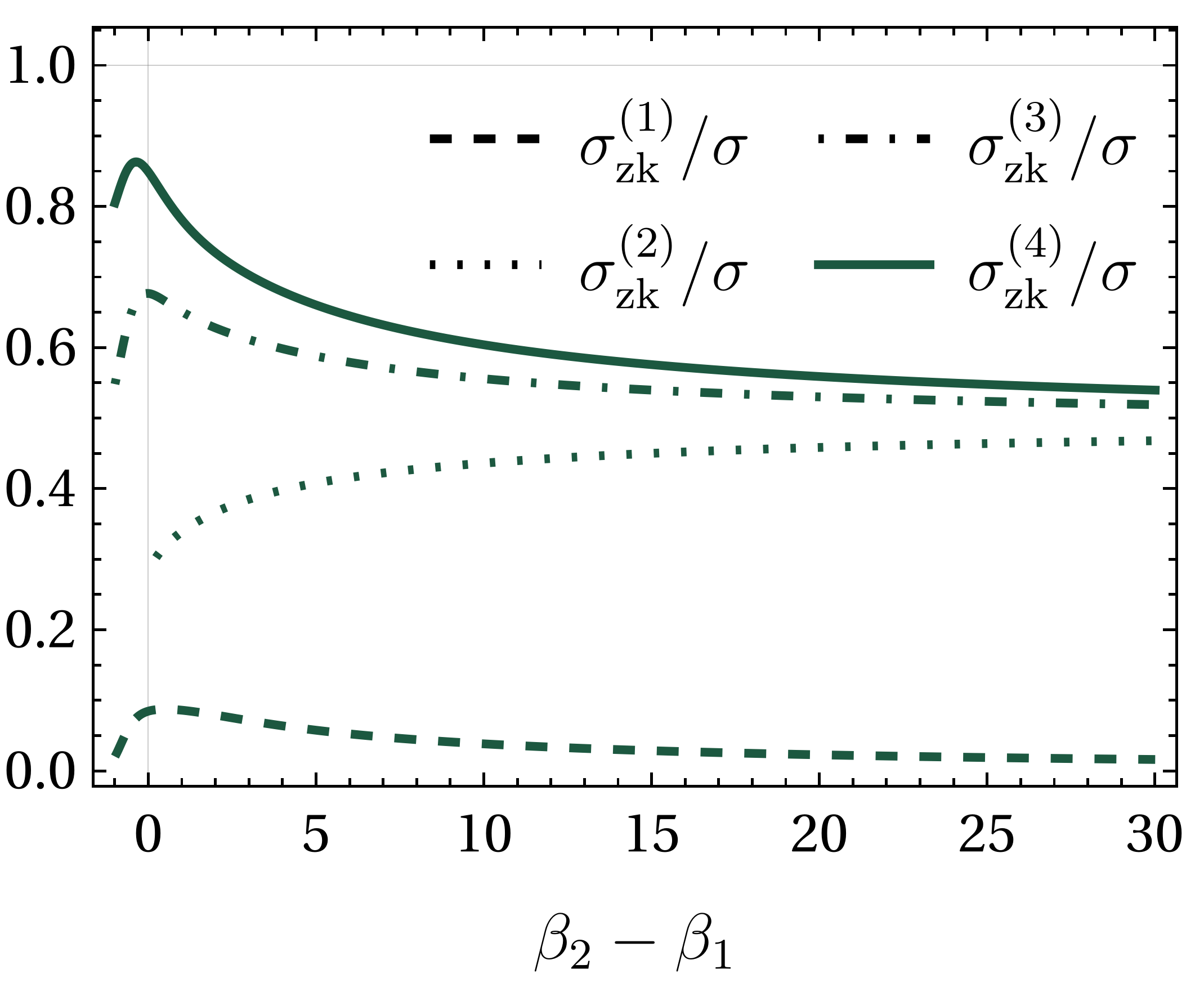
Figure 4: The EPR estimators based on $\sigma_{\text{zk}}$ with $\beta_{2}\in[0,31]$, all other parameters are equal to those of Fig. 3.

In the case of reservoirs with different temperatures, the non-isothermal scenario, the affinities will not be the same throughout the distinct cycles and the method of $\sigma_{\text{ti}}$ does not apply. For instance, the cycle between 00 and 01 will have affinity $\epsilon_{u}(\beta_{2}-\beta_{1})+\beta_{1}\mu_{1}-\beta_{2}\mu_{2}$, while between 10 and 11 it is $(\epsilon_{u}+\Delta\epsilon)(\beta_{2}-\beta_{1})+\beta_{1}\mu_{1}-\beta_{2}\mu_{2}$. It is evident that the same affinity case is recovered when $\beta_{1}=\beta_{2}$. Each affinity cannot be measured since the occurrence of individual cycles cannot be resolved from the multifilar events of particle exchanges, although it would be possible if energy transfers were also monitored. Also, there is an affinity $\Delta\epsilon(\beta_{1}-\beta_{3})$ related to the cycle $00\xrightarrow{1}01\xrightarrow{3}11\xrightarrow{1}10\xrightarrow{3}00$ that contributes to the EPR and cannot be obtained from multifilar events. Figure 4 shows the EPR lower bound using the zero-knowledge estimator with the same convention as in Fig. 3. Changing one of the temperatures has a nontrivial influence on the estimators, but the main features are preserved: It is still a lower bound and the addition of reservoirs makes it tighter. $D_{x}$ and $D_{t}$ are able to detect nonequilibrium behavior in this case.

In the presence of transitions not mediated by any of the reservoirs, such as a possible electron hops between quantum-dots $01\leftrightarrow 10$, the estimator $\sigma_{\text{zk}}$ would still provide a lower bound, and the detectors $D_{x}$ and $D_{t}$ would still be nonnegative and vanish at equilibrium. The sequence of some particular events would still measure the affinities using Eq. (28), however the currents will change and there will be an additional contribution to the EPR, and not only $\sigma_{\text{ti}}$ no longer provides the exact EPR, but it can also overestimate it.

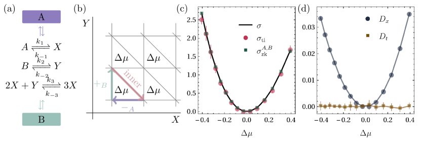
Figure 5: (a) Reactions of the considered Brusselator model and reservoirs chemostating species $A$ and $B$; (b) state space with degenerate affinities $\Delta\mu$ and highlighted multifilar events that can be observed from the chemostats and the internal event; (c) In terms of affinity $\Delta\mu$, EPR, topology-informed estimator, and zero-knowledge estimators for the observation of both reservoirs; (d) Nonequilibrium detectors evaluated with the statistics of reservoirs $A$ and $B$. More details in the main text.

V.2 Brusselator

The second model considered is composed of three chemical reactions, two fluctuating chemical species $X$ and $Y$, and two species whose concentrations are fixed by chemostats [see Fig. 5(a)]. It is a simplified version of the Brusselator model  Fritz et al. (2020); Nicolis and Prigogine (1977); Qian et al. (2002) that is largely studied due to its nontrivial behavior, such as the presence of a limit cycle and chemical oscillations emerging through a phase transition Qian et al. (2002); Nguyen et al. (2018). The state space is the infinite 2D lattice of concentrations of $X$ and $Y$ with reactions translating into horizontal ($k_{\pm 1}$), vertical ($k_{\pm 2}$), and diagonal ($k_{\pm 3}$) transitions. The affinity is given by $\Delta\mu=\ln([B]k_{2}k_{-1}k_{3}/[A]k_{-2}k_{1}k_{-3})$ and the entropy production is $\sigma=J\Delta\mu$, with $J$ being the current from one of the chemostats to the reservoir. For the numerical simulations of this model, we adopt the following parameters: $k_{1}=3$, $k_{-1}=2$, $k_{2}=2$, $k_{-2}=3$, $k_{3}=3$, $k_{-3}=1$, $[B]=10$, $V=2$ and $[A]$ is changed from 9 to 20. The propensities $k_{\pm\rho}$ translate into transition rates according to the rule of mass-action kinetics:

$$r_{1}=k_{1}[A] \qquad r_{-1}=k_{-1}[X]$$

$$r_{2}=k_{2}[B] \qquad r_{-2}=k_{-2}[Y]$$

$$r_{3}=k_{3}\frac{[X][X-1][Y]}{V^{2}} \qquad r_{-3}=k_{-3}\frac{[X][X-1][X-2]}{V^{2}}$$ (34)

where $V$ is the volume of the vessel where reactions take place.

As seen in Fig. 5(b), the state space has an infinite number of cycles, all with affinity $\Delta\mu$ that can be univocally related to the sequence of reactions $\{-_{1},+_{2},+_{3}\}$. The first two types of reactions give rise to multifilar events that can be monitored as exchanges of chemostatted species between system and reservoir. If we assume that the internal reactions $k_{\pm 3}$ are also monitored, then the affinity can be empirically estimated by $\ln P(-_{A},+_{B},+_{I})/P(-_{I},-_{B},+_{A})$; then the EPR is obtained by multiplying the estimated affinity by the current from one of the reservoirs to the system. This result is shown in Fig. 5(c) through numerical simulations and agrees with the exact EPR. However, in general, the internal transitions do not give rise to an observable event, thus we now turn to the other estimators.

When the only observables are changes in the chemostats, the zero-knowledge estimator $\sigma_{\text{zk}}$ can be used to bound the EPR from below. Figure 5(c) shows the bound $\sigma_{\text{zk}}^{A,B}$ when both chemostats are monitored. As a proof of concept, this lower bound is tight for the studied parameters, in contrast to other estimators that can be orders of magnitude loose. We remind that they require no knowledge about propensities $k_{\pm\rho}$ or the chemostatted concentrations $[A]$ and $[B]$, and they also do not involve assessment of the affinity $\Delta\mu$, these bounds only concern the promptly accessible statistics of changes in the chemostats and directly measure the irreversibility of individual multifilar events.

Since $\Delta\mu$ is the only affinity of the model, the system is in equilibrium when it vanishes and all estimators/detectors should vanish for $\Delta\mu=0$. Lastly, Fig. 5(d) shows the nonequilibrium detectors $D_{x}$ and $D_{t}$ evaluated from the statistics of both chemostats. The values of $D_{x}$ indicate the presence of nonequilibrium behavior when $\Delta\mu\neq 0$ and vanish otherwise. Its waiting-times counterpart, $D_{t}$, fails in detecting nonequilibrium behavior even in the presence of a nonzero affinity.

VI Discussion

In summary, we extend the framework of transition-based coarse-graining to the case of multifilar events, which represent a large class of systems and is commonplace in experiments. We present methods to detect and quantify nonequilibrium from the available information: an EPR lower bound $\sigma_{\text{zk}}$, detectors of nonequilibrium behavior based on sequences of events $D_{x}$ and waiting-times $D_{t}$, and an EPR estimator $\sigma_{\text{ti}}$ that benefits from previously known topological information. Contrary to textbook approaches, these quantities deal with minimal information from the systems: $\sigma_{\text{zk}}$, $D_{x}$ and $D_{t}$ are model-free, and $\sigma_{\text{ti}}$ only uses topological information, bypassing the need to estimate transition rates. Therefore, they are relevant for bridging experiments, where partial information is the rule, to the toolbox of nonequilibrium thermodynamics. Similarly, they can be used to validate proposed models.

It is possible to bound the EPR from below through the probabilities of individual events, and although a semi-Markov-type estimator that uses conditional probabilities is useful for detecting nonequilibrium, it is shown to not establish a lower bound (unless the system falls in a given class Ertel and Seifert (2023)). It would be important to devise estimators that benefit from conditional probabilities since they can entail more information and account for waiting-time distributions. Beyond them, inferring EPR from non-Markovian trajectories becomes computationally expensive and available techniques can be intricate. It would be relevant to specialize non-Markovian methods for the case of multifilar events, possibly constraining to physical scenarios such as the exchange of particles and energies with reservoirs.

We have seen that $D_{t}$ can detect nonequilibrium behavior through asymmetries in waiting-time distributions even when the current of the monitored reservoir vanishes, at the same time this estimator is always compatible with zero for the simplified Brusselator model. It would be interesting to understand the mechanisms behind its behavior and the classes of systems in which $D_{t}$ becomes ineffective.

As illustrated by the double quantum-dot model, only two reservoir currents must be monitored if the affinities are known, but $\sigma_{\text{zk}}$ gets tighter when all four reservoirs are monitored. This is due to the lack of physical information in this bound. Another possible extension of the present results is to account for possible physical symmetries owing to known conservation laws. Also, to move from the detection of cycle affinities to thermodynamic forces, to understand the role of conserved quantities in identifying detectable families of cycles, and to explore the case of continuous multifilar events where energy exchanges are detected under limited resolution.

Further examples of setups where the present results can be relevant include pulling experiments involving more than one DNA hairpin in series, detection of ligand binding while distinct receptors cannot be resolved, emission of photons without detecting which atoms are in the excited state, observed RNA elongation from unresolved transcription loci, molecular motors with many mechanisms driving the mechanical steps, more convoluted chemical reaction networks, and an unknown electronic device between two monitored leads. Also, in setups where there is no assumed Markov model or the model is under question, employing the developed model-free estimators can reveal otherwise hidden properties of the system from experimentally accessible data.

VII Data Availability Statement

The codes and data used to generate the analytical and numerical results of the present work are available and described in the repository Harunari (2024).

VIII Acknowledgments

We thank Massimiliano Esposito for useful discussions. This research was supported by the project INTER/FNRS/20/15074473 funded by F.R.S.-FNRS (Belgium) and FNR (Luxembourg).

Appendix A Auxiliary process with multifilarity

The joint probability density of the next multifilar event and its waiting-time, conditioned on the previous event, can be obtained by solving a first-transition time problem. The solution is a simple extension of the proof in Appendix A of Ref. Harunari et al. (2022), but the matrix $\mathbf{L}$ defined therein now has the contribution of more than one transition per element. The proof sketch is similar, and we present it here for consistency.

For a Markov process with generator $\mathbf{R}$, we define multifilar events $x$ that immediately occur when a transition $\ell\in\theta^{-1}x$ is performed. The auxiliary process is established by the introduction of an absorbing state for each event, and all transitions that generate these events are redirected towards its respective absorbing state Sekimoto (2021). The generator of the auxiliary process is the block matrix

$$\mathbf{R}_{\text{aux}}=\left(\begin{array}[]{c@{}|c@{}}\mathbf{S}&0\\ \hline\cr\mathbf{L}&0\\ \end{array}\right),$$ (35)

where $\mathbf{S}$ is the survival matrix in Eq. (7) and

$$[\mathbf{L}]_{x,j}\coloneqq\sum_{\ell\in\theta^{-1}x}r_{\ell}\delta_{j,\mathsf{s}(\ell)}$$ (36)

with each row $x$ representing one of the events. Notice that their order is not relevant. The formal solution of the master equation, $\mathbf{p}(t)=\exp(t\mathbf{R})\mathbf{p}(0)$, requires the matrix exponential of the generator, the propagator, that for the auxiliary dynamics reads

$$\exp(t\mathbf{R}_{\text{aux}})=\left(\begin{array}[]{c@{}|c@{}}\exp(t\mathbf{S})&0\\ \hline\cr\mathbf{L}\mathbf{S}^{-1}[\exp(t\mathbf{S}-1)]&0\\ \end{array}\right).$$ (37)

The probability that the process evolves during time $t$ without reaching a particular absorbing state associated with $x$ is known as its survival probability. Conditioning on a particular initial distribution $\mathbf{p}_{\text{aux}}^{0}$, the survival probability is

$$\mathbb{S}(t,x|\mathbf{p}_{\text{aux}}^{0})=1-[\exp(t\mathbf{R}_{\text{aux}})\mathbf{p}_{\text{aux}}^{0}]_{x}.$$ (38)

Assuming that the initial distribution has entries zero in the rows associated with sinks, which is the relevant case here, it is a vector with first entries $\mathbf{p}^{0}$ that is a valid distribution in the original state space. Hence, the only elements that will be relevant come from the bottom-left block of Eq. (37). The first-passage time is obtained as minus the time derivative of the survival probability, and the joint probability we aim at is precisely the first-passage time, therefore

$$P(x,t|\mathbf{p}_{\text{aux}}^{0})=\sum_{\ell\in\theta^{-1}x}r_{\ell}[\exp(t\mathbf{S})\mathbf{p}^{0}]_{\mathsf{s}(\ell)}.$$ (39)

Now, if the process is conditioned on the previous multifilar event, $\mathbf{p}^{0}\to\mathbf{p}_{|x}$. Finally, the joint probability density to perform an event $x\raise 1.72218pt\hbox{$\scriptstyle\prime$}$ after waiting-time $t$ becomes equivalent to Eq. (9).

Appendix B Invertibility and convergence of the auxiliary process

Here, we prove that the propagator of the survival process $\exp(t\mathbf{S})$ is finite at long times, and that $\mathbf{S}^{-1}$ exists. First, we note that, since probabilities have to be preserved, $\mathbf{1}\cdot\mathbf{p}=1$, the columns of a continuous-time Markov chain generator $\mathbf{R}$ sum to zero. It can be seen as a property of the master equation’s formal solution; consider a small enough $\delta t$, then

$$\mathbf{1}\cdot\left[\mathbf{p}(t+\delta t)\right] =\mathbf{1}\cdot\left[e^{(t+\delta t)\mathbf{R}}\mathbf{p}(t)\right]$$

$$=\mathbf{1}\cdot\left[\left(\mathbf{I}+\delta t\mathbf{R}+\mathcal{O}[\delta t^{2}]\right)\mathbf{p}(t)\right]$$

$$=1+\delta t\left(\mathbf{1}\cdot\mathbf{R}\right)\mathbf{p}(t)=1,$$ (40)

where we dropped the higher-order contributions. Second, if the process is supported by an irreducible network, the generator $\mathbf{R}$ has a non-degenerate eigenvalue equal to zero, and its respective eigenvector has non-zero entries describing the stationary distribution. This is a consequence of applying the Perron-Frobenius theorem to a discretized version of the Markov chain.

The Gershgorin circle theorem Gershgorin (1931) states that all eigenvalues $\lambda$ of a matrix $\mathbf{R}$ lie within at least one disc $D_{i}(\mathbf{R})\subseteq\mathbb{C}$ in the complex plane, where each disk is centered at the diagonal element $R_{ii}$ and has a radius equal to the sum of the non-diagonal elements $\sum_{j\neq i}R_{ji}$. Since every diagonal element of a generator is equal to minus the sum of non-diagonal entries in its column, every $D_{i}(\mathbf{R})$ is contained in the non-positive side of the real axis. Therefore, the real part of all eigenvalues is non-positive, in agreement with Perron-Frobenius.

By construction, matrices $\mathbf{R}$ and $\mathbf{S}$ share the same diagonal elements (exit rates), but the columns of $\mathbf{S}$ will sum to a value smaller than or equal to the sum of those of $\mathbf{R}$. Therefore, one or more of the Gershgorin discs $D_{i}(\mathbf{S})$ are shrunk versions of $D_{i}(\mathbf{R})$, see Fig. 6. Hence the real part of all eigenvalues of $\mathbf{S}$ are also non-negative.

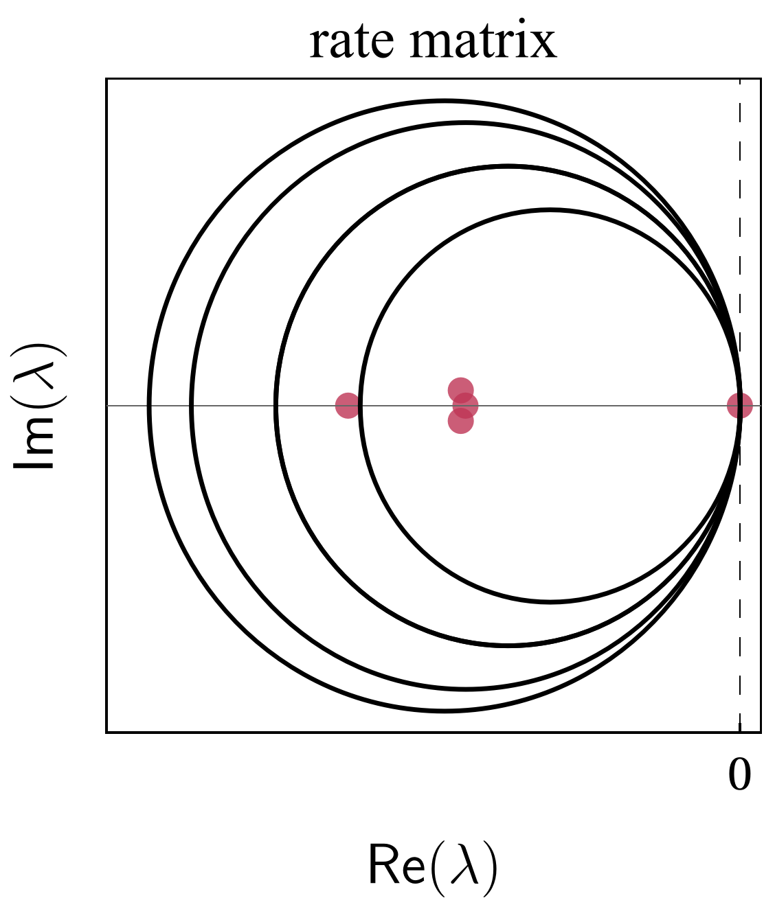
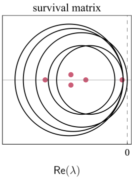
Figure 6: Gershgorin discs (black) and eigenvalues (red dots) for the rate matrix $\mathbf{R}$ (left) and the survival matrix $\mathbf{S}$ (right). The state space has 5 states and is fully connected, to construct $\mathbf{S}$ we consider two visible transitions.

Notice that the eigenvalues are functions of the matrix elements. The process of constructing $\mathbf{S}$ from $\mathbf{R}$ involves reducing some of its values and therefore changing the eigenvalues. Since the new eigenvalues have to fall in one of the Gershgorin discs, which are all in the non-positive side, the eigenvalue with the largest real part will acquire a negative real part, which is a sufficient condition for the invertibility. It is worth commenting that there are characteristic polynomial-preserving transformations, such as swapping rows or columns, which are not involved in the survival matrix. In addition, similarity transformations would leave the eigenvalues unchanged, so if there exists an invertible $\mathbf{P}$ such that $\mathbf{S}=\mathbf{P}^{-1}\mathbf{R}\mathbf{P}$, then $\mathbf{S}$ will not be invertible. However, it would require a very particular symmetry to achieve such a similarity relation, which is unlikely to be possible under the condition of irreducibility.

Finally, Sylvester’s formula states that for a diagonalizable matrix $\mathbf{S}$

$$\lim_{t\to\infty}e^{t\mathbf{S}}=\lim_{t\to\infty}\sum_{k}A_{k}e^{t\lambda_{k}}=\lim_{t\to\infty}A_{\tilde{k}}e^{t\lambda_{\tilde{k}}},$$ (41)

where the sum spans through all eigenvalues and $\tilde{k}$ indexes the eigenvalue with largest real part. When the largest eigenvalue of $\mathbf{S}$ is negative, Eq. (41) vanishes. In contrast, if the largest eigenvalue is zero, $e^{t\mathbf{S}}\to A_{\tilde{k}}$, which means that the propagation through hidden pathways does not leak all its probability and the system can get stuck in a hidden part, never performing a new visible transition.

References

- Fang et al. (2019) Xiaona Fang, Karsten Kruse, Ting Lu, and Jin Wang, “Nonequilibrium physics in biology,” Reviews of Modern Physics 91, 045004 (2019).
- Gnesotto et al. (2018) F. S. Gnesotto, F. Mura, J. Gladrow, and C. P. Broedersz, “Broken detailed balance and non-equilibrium dynamics in living systems: A review,” Reports on Progress in Physics 81, 066601 (2018).
- Zoller et al. (2022) Benjamin Zoller, Thomas Gregor, and Gašper Tkačik, “Eukaryotic gene regulation at equilibrium, or non?” Current Opinion in Systems Biology 31, 100435 (2022).
- Hartich et al. (2015) David Hartich, Andre C. Barato, and Udo Seifert, “Nonequilibrium sensing and its analogy to kinetic proofreading,” New Journal of Physics 17, 055026 (2015).
- Yang et al. (2021) Xingbo Yang, Matthias Heinemann, Jonathon Howard, Greg Huber, Srividya Iyer-Biswas, Guillaume Le Treut, Michael Lynch, Kristi L. Montooth, Daniel J. Needleman, Simone Pigolotti, Jonathan Rodenfels, Pierre Ronceray, Sadasivan Shankar, Iman Tavassoly, Shashi Thutupalli, Denis V. Titov, Jin Wang, and Peter J. Foster, “Physical bioenergetics: Energy fluxes, budgets, and constraints in cells,” Proceedings of the National Academy of Sciences 118, e2026786118 (2021).
- Jarzynski (1997) C. Jarzynski, “Nonequilibrium equality for free energy differences,” Phys. Rev. Lett. 78, 2690–2693 (1997).
- Crooks (1999) Gavin E. Crooks, “Entropy production fluctuation theorem and the nonequilibrium work relation for free energy differences,” Phys. Rev. E 60, 2721–2726 (1999).
- Evans et al. (1993) Denis J. Evans, E. G. D. Cohen, and G. P. Morriss, “Probability of second law violations in shearing steady states,” Phys. Rev. Lett. 71, 2401–2404 (1993).
- Barato and Seifert (2015) Andre C. Barato and Udo Seifert, “Thermodynamic uncertainty relation for biomolecular processes,” Phys. Rev. Lett. 114, 158101 (2015).
- Horowitz and Gingrich (2020) Jordan M Horowitz and Todd R Gingrich, “Thermodynamic uncertainty relations constrain non-equilibrium fluctuations,” Nature Physics 16, 15–20 (2020).
- Falasco and Esposito (2020) Gianmaria Falasco and Massimiliano Esposito, “Dissipation-time uncertainty relation,” Phys. Rev. Lett. 125, 120604 (2020).
- Shiraishi et al. (2018) Naoto Shiraishi, Ken Funo, and Keiji Saito, “Speed limit for classical stochastic processes,” Phys. Rev. Lett. 121, 070601 (2018).
- Owen et al. (2020) Jeremy A. Owen, Todd R. Gingrich, and Jordan M. Horowitz, “Universal thermodynamic bounds on nonequilibrium response with biochemical applications,” Phys. Rev. X 10, 011066 (2020).
- Basu and Maes (2015) Urna Basu and Christian Maes, “Nonequilibrium response and frenesy,” Journal of Physics: Conference Series 638, 012001 (2015).
- Kawaguchi and Nakayama (2013) Kyogo Kawaguchi and Yohei Nakayama, “Fluctuation theorem for hidden entropy production,” Phys. Rev. E 88, 022147 (2013).
- Herpich et al. (2020) Tim Herpich, Kamran Shayanfard, and Massimiliano Esposito, “Effective thermodynamics of two interacting underdamped Brownian particles,” Physical Review E 101, 022116 (2020).
- Manikandan et al. (2020) Sreekanth K. Manikandan, Deepak Gupta, and Supriya Krishnamurthy, “Inferring entropy production from short experiments,” Phys. Rev. Lett. 124, 120603 (2020).
- Busiello and Pigolotti (2019) Daniel Maria Busiello and Simone Pigolotti, “Hyperaccurate currents in stochastic thermodynamics,” Phys. Rev. E 100, 060102 (2019).
- Li et al. (2019) Junang Li, Jordan M Horowitz, Todd R Gingrich, and Nikta Fakhri, “Quantifying dissipation using fluctuating currents,” Nature communications 10, 1666 (2019).
- Van Vu et al. (2020) Tan Van Vu, Van Tuan Vo, and Yoshihiko Hasegawa, “Entropy production estimation with optimal current,” Phys. Rev. E 101, 042138 (2020).
- Skinner and Dunkel (2021) Dominic J Skinner and Jörn Dunkel, “Improved bounds on entropy production in living systems,” Proceedings of the National Academy of Sciences 118, e2024300118 (2021).
- Shiraishi and Sagawa (2015) Naoto Shiraishi and Takahiro Sagawa, “Fluctuation theorem for partially masked nonequilibrium dynamics,” Phys. Rev. E 91, 012130 (2015).
- Bisker et al. (2017) Gili Bisker, Matteo Polettini, Todd R Gingrich, and Jordan M Horowitz, “Hierarchical bounds on entropy production inferred from partial information,” Journal of Statistical Mechanics: Theory and Experiment 2017, 093210 (2017).
- Ehrich (2021) Jannik Ehrich, “Tightest bound on hidden entropy production from partially observed dynamics,” Journal of Statistical Mechanics: Theory and Experiment 2021, 083214 (2021).
- Blom et al. (2023) Kristian Blom, Kevin Song, Etienne Vouga, Aljaž Godec, and Dmitrii E. Makarov, “Milestoning estimators of dissipation in systems observed at a coarse resolution: When ignorance is truly bliss,” (2023), arXiv:2310.06833 [cond-mat.stat-mech] .
- Roldán and Parrondo (2010) Édgar Roldán and Juan M. R. Parrondo, “Estimating dissipation from single stationary trajectories,” Phys. Rev. Lett. 105, 150607 (2010).
- Martínez et al. (2019) Ignacio A Martínez, Gili Bisker, Jordan M Horowitz, and Juan MR Parrondo, “Inferring broken detailed balance in the absence of observable currents,” Nature communications 10, 3542 (2019).
- Esposito (2012) Massimiliano Esposito, “Stochastic thermodynamics under coarse graining,” Phys. Rev. E 85, 041125 (2012).
- Bo and Celani (2014) Stefano Bo and Antonio Celani, “Entropy Production in Stochastic Systems with Fast and Slow Time-Scales,” Journal of Statistical Physics 154, 1325–1351 (2014).
- Rahav and Jarzynski (2007) Saar Rahav and Christopher Jarzynski, “Fluctuation relations and coarse-graining,” Journal of Statistical Mechanics: Theory and Experiment 2007, P09012 (2007).
- Harunari et al. (2022) Pedro E. Harunari, Annwesha Dutta, Matteo Polettini, and Édgar Roldán, “What to learn from a few visible transitions’ statistics?” Phys. Rev. X 12, 041026 (2022).
- van der Meer et al. (2022) Jann van der Meer, Benjamin Ertel, and Udo Seifert, “Thermodynamic inference in partially accessible markov networks: A unifying perspective from transition-based waiting time distributions,” Phys. Rev. X 12, 031025 (2022).
- van der Meer et al. (2023) Jann van der Meer, Julius Degünther, and Udo Seifert, “Time-resolved statistics of snippets as general framework for model-free entropy estimators,” Phys. Rev. Lett. 130, 257101 (2023).
- Harunari et al. (2023) Pedro E. Harunari, Alberto Garilli, and Matteo Polettini, “Beat of a current,” Phys. Rev. E 107, L042105 (2023).
- Garilli et al. (2023) Alberto Garilli, Pedro E. Harunari, and Matteo Polettini, “Fluctuation relations for a few observable currents at their own beat,” (2023), arXiv:2312.07505 [cond-mat.stat-mech] .
- Maes (2017) Christian Maes, “Frenetic Bounds on the Entropy Production,” Physical Review Letters 119, 160601 (2017).
- Berezhkovskii and Makarov (2019) Alexander M. Berezhkovskii and Dmitrii E. Makarov, “On the forward/backward symmetry of transition path time distributions in nonequilibrium systems,” The Journal of Chemical Physics 151, 065102 (2019).
- Cristadoro et al. (2023) Giampaolo Cristadoro, Mirko Degli Esposti, Vojkan Jakšić, and Renaud Raquépas, “Recurrence times, waiting times and universal entropy production estimators,” Letters in Mathematical Physics 113, 19 (2023).
- Singh and Proesmans (2023) Prashant Singh and Karel Proesmans, “Inferring entropy production from time-dependent moments,” (2023), arXiv:2310.16627 [cond-mat.stat-mech] .
- Ferri-Cortés et al. (2023) Mar Ferri-Cortés, Jose A. Almanza-Marrero, Rosa López, Roberta Zambrini, and Gonzalo Manzano, “Entropy production and fluctuation theorems for monitored quantum systems under imperfect detection,” (2023), arXiv:2308.08491 [quant-ph] .
- Liang and Pigolotti (2023) Shiling Liang and Simone Pigolotti, “Thermodynamic bounds on time-reversal asymmetry,” (2023), arXiv:2308.14497 [cond-mat].
- Ertel and Seifert (2023) Benjamin Ertel and Udo Seifert, “An estimator of entropy production for partially accessible markov networks based on the observation of blurred transitions,” (2023), arXiv:2312.08246 [cond-mat.stat-mech] .
- Degünther et al. (2023) Julius Degünther, Jann van der Meer, and Udo Seifert, “Fluctuating entropy production on the coarse-grained level: Inference and localization of irreversibility,” arXiv preprint arXiv:2309.07665 (2023), https://doi.org/10.48550/arXiv.2309.07665.
- Yu et al. (2021) Qiwei Yu, Dongliang Zhang, and Yuhai Tu, “Inverse Power Law Scaling of Energy Dissipation Rate in Nonequilibrium Reaction Networks,” Physical Review Letters 126, 080601 (2021).
- Baiesi et al. (2023) Marco Baiesi, Gianmaria Falasco, and Tomohiro Nishiyama, “Effective estimation of entropy production with lacking data,” (2023), arxiv:2305.04657 [cond-mat] .
- Hartich and Godec (2021) David Hartich and Aljaž Godec, “Emergent Memory and Kinetic Hysteresis in Strongly Driven Networks,” Physical Review X 11, 041047 (2021).
- Lucente et al. (2023) D. Lucente, M. Viale, A. Gnoli, A. Puglisi, and A. Vulpiani, “Revealing the Nonequilibrium Nature of a Granular Intruder: The Crucial Role of Non-Gaussian Behavior,” Physical Review Letters 131, 078201 (2023).
- Gnesotto et al. (2020) Federico S. Gnesotto, Grzegorz Gradziuk, Pierre Ronceray, and Chase P. Broedersz, “Learning the non-equilibrium dynamics of Brownian movies,” Nature Communications 11, 5378 (2020).
- Lynn et al. (2022) Christopher W. Lynn, Caroline M. Holmes, William Bialek, and David J. Schwab, “Decomposing the Local Arrow of Time in Interacting Systems,” Physical Review Letters 129, 118101 (2022).
- Tan et al. (2021) Tzer Han Tan, Garrett A. Watson, Yu-Chen Chao, Junang Li, Todd R. Gingrich, Jordan M. Horowitz, and Nikta Fakhri, “Scale-dependent irreversibility in living matter,” (2021), arxiv:2107.05701 [cond-mat, physics:physics] .
- Lucente et al. (2022) D. Lucente, A. Baldassarri, A. Puglisi, A. Vulpiani, and M. Viale, “Inference of time irreversibility from incomplete information: Linear systems and its pitfalls,” Physical Review Research 4, 043103 (2022).
- Walldorf et al. (2018) Nicklas Walldorf, Ciprian Padurariu, Antti-Pekka Jauho, and Christian Flindt, “Electron waiting times of a cooper pair splitter,” Phys. Rev. Lett. 120, 087701 (2018).
- Landi (2021) Gabriel T. Landi, “Waiting time statistics in boundary-driven free fermion chains,” Phys. Rev. B 104, 195408 (2021).
- Cuetara and Esposito (2015) Gregory Bulnes Cuetara and Massimiliano Esposito, “Double quantum dot coupled to a quantum point contact: a stochastic thermodynamics approach,” New Journal of Physics 17, 095005 (2015).
- Viisanen et al. (2015) Klaara L Viisanen, Samu Suomela, Simone Gasparinetti, Olli-Pentti Saira, Joachim Ankerhold, and Jukka P Pekola, “Incomplete measurement of work in a dissipative two level system,” New Journal of Physics 17, 055014 (2015).
- Sánchez et al. (2019) Rafael Sánchez, Janine Splettstoesser, and Robert S. Whitney, “Nonequilibrium system as a demon,” Phys. Rev. Lett. 123, 216801 (2019).
- Freitas and Esposito (2021) Nahuel Freitas and Massimiliano Esposito, “Characterizing autonomous maxwell demons,” Phys. Rev. E 103, 032118 (2021).
- Rao and Esposito (2018a) Riccardo Rao and Massimiliano Esposito, “Conservation laws and work fluctuation relations in chemical reaction networks,” The Journal of chemical physics 149 (2018a), https://doi.org/10.1063/1.5042253.
- Note (1) Connecting to the notation of Ref. Harunari et al. (2022), can be expressed as .
- Sekimoto (2021) Ken Sekimoto, “Derivation of the first passage time distribution for markovian process on discrete network,” (2021), arXiv:2110.02216 [cond-mat.stat-mech] .
- Schnakenberg (1976) J. Schnakenberg, “Network theory of microscopic and macroscopic behavior of master equation systems,” Rev. Mod. Phys. 48, 571–585 (1976).
- Note (2) Empirical estimation of the divergence of continuous variables presents convergence problems, the reader may refer to the code in Harunari and Yssou (2022) for an unbiased estimator.
- Falasco and Esposito (2021) Gianmaria Falasco and Massimiliano Esposito, “Local detailed balance across scales: From diffusions to jump processes and beyond,” Physical Review E 103, 042114 (2021).
- Note (3) Local detailed balance for a given transition reads , with the entropy flux generated by , and the affinity of a cycle becomes .
- Polettini et al. (2016) Matteo Polettini, Gregory Bulnes-Cuetara, and Massimiliano Esposito, “Conservation laws and symmetries in stochastic thermodynamics,” Physical Review E 94, 052117 (2016).
- Rao and Esposito (2018b) Riccardo Rao and Massimiliano Esposito, “Conservation laws shape dissipation,” New Journal of Physics 20, 023007 (2018b).
- Avanzini et al. (2023) Francesco Avanzini, Massimo Bilancioni, Vasco Cavina, Sara Dal Cengio, Massimiliano Esposito, Gianmaria Falasco, Danilo Forastiere, Nahuel Freitas, Alberto Garilli, Pedro E. Harunari, Vivien Lecomte, Alexandre Lazarescu, Shesha G. Marehalli Srinivas, Charles Moslonka, Izaak Neri, Emanuele Penocchio, William D. Piñeros, Matteo Polettini, Adarsh Raghu, Paul Raux, Ken Sekimoto, and Ariane Soret, “Methods and Conversations in (Post)Modern Thermodynamics,” (2023), arXiv:2311.01250 [cond-mat].
- Borrelli et al. (2015) Massimo Borrelli, Jonne V. Koski, Sabrina Maniscalco, and Jukka P. Pekola, “Fluctuation relations for driven coupled classical two-level systems with incomplete measurements,” Phys. Rev. E 91, 012145 (2015).
- Fritz et al. (2020) Jonas H. Fritz, Basile Nguyen, and Udo Seifert, “Stochastic thermodynamics of chemical reactions coupled to finite reservoirs: A case study for the Brusselator,” J. Chem. Phys. 152, 235101 (2020).
- Nicolis and Prigogine (1977) G. Nicolis and I. Prigogine, Self-Organization in Nonequilibrium Systems: From Dissipative Structures to Order Through Fluctuations, A Wiley-Interscience publication (Wiley, 1977).
- Qian et al. (2002) Hong Qian, Saveez Saffarian, and Elliot L Elson, “Concentration fluctuations in a mesoscopic oscillating chemical reaction system,” Proceedings of the National Academy of Sciences 99, 10376–10381 (2002).
- Nguyen et al. (2018) Basile Nguyen, Udo Seifert, and Andre C Barato, “Phase transition in thermodynamically consistent biochemical oscillators,” The Journal of Chemical Physics 149 (2018).
- Harunari (2024) Pedro E. Harunari, “Multifilarevents,” https://github.com/pedroharunari/MultifilarEvents (2024).
- Gershgorin (1931) S. Gershgorin, “über die abgrenzung der eigenwerte einer matrix,” Bull. Acad. Sci. URSS , 749–754 (1931).
- Harunari and Yssou (2022) Pedro E. Harunari and Ariel Yssou, “Kullback-leibler divergence estimation algorithm and inter-transition times application,” https://github.com/pedroharunari/KLD_estimation (2022).