Linear optics and the problem of Bell-like state discrimination

Abstract

A linear optics-based scheme to implement various quantum information processing tasks is of paramount importance due to ease of implementation and low noise. Many information-theoretic tasks depend on the successful discrimination of Bell states. A no-go theorem has been proved in literature which tells that it is not possible to perfectly discriminate among the four Bell states by restricting measurement apparatus to linear optical elements. The success probability is only $50\%$. Through using extra resources such as hyper entanglement, ancillary entanglement, and even a minimum amount of non-linearity complete Bell-state discrimination can be achieved. The success probability for Bell-like state discrimination is only $25\%$. We find that this can be boosted up to $50\%$ using hyperentanglement in polarization, momentum, or OAM degrees of freedom of the photons which is in contrast to the Bell-state discrimination scenario where $100\%$ can be achieved. Furthermore, we find that by using correlation in time of the photons all four Bell states can be distinguished with $100\%$ success probability while for the Bell-like state discrimination, it strictly lies between $25\%$ and $50\%$ depending on the state parameter with only three Bell-like states being distinguishable. We also observe a similar contrast when we use ancillary entangled photons. While the success probability for all four Bell-state discrimination increases as $1-\frac{1}{2^{N}}$ where N is the number of ancillary photons for Bell-like states it depends again on the state parameters and can be less than $25\%$ in some cases. Also adding further ancillary photons decreases the success probability. We then show that using non-linear gadgets namely SFG $100\%$ success probability can be achieved even for Bell-like state discrimination.

I Introduction

Linear optics-based schemes are very promising candidates for building devices for computation[2] and communication[3] purposes. Photons are very robust to noise. They have large coherence times. It is also known that KLM scheme offers a universal model of quantum computing just using linear-optical elements[4, 5, 6]. Any N-port unitary operation can be implemented using an array of $\frac{N(N-1)}{2}$ beam splitters[7, 8]. This number grows only quadratically with N, thus giving a realistic hope for implementing various quantum operations using linear optical elements. But there are fundamental limitations on what kind of operations are possible to implement deterministically if we stick to linear optics only[9, 10, 11, 12]. A very simple but important example of the inadequacy of the linear optical-based schemes is that it is unable to distinguish among maximally entangled Bell states if no ancillary photons and resources are not allowed[1]. By relaxing the constraints of perfect Bell state discrimination by allowing it to fail with some probability it can be proved that the maximum success probability of this scheme is $50\%$ given that there are zero auxiliary photons and no conditional measurements[13]. Thus linear optics-based schemes are restrictive in that sense. But various information-theoretic tasks namely quantum teleportation[14], entanglement swapping[15, 16], super-dense coding[17, 18], etc. depend on the successful discrimination of Bell states. Hence it is important to look for ways of increasing the probability of successful Bell state discrimination from $50\%$. As it turns it can be increased by using extra ancillary photons[19], hyperentanglement[20, 21, 17], or some minimal amount of non-linearity[22, 23]. All these methods can boost the success probability to $100\%$.

A more general version of this problem is distinguishing among the Bell-like states unambiguously. On the same lines as the treatment in [13] it was shown in [24] that the optimal success probability for discrimination of Bell-like states without using any ancillary photons and conditional measurements is $25\%$. In practical scenarios, one might not be provided with Bell states. Instead, a weaker resource, namely non-maximally entangled states, might be present. Thus it is important to distinguish among non-maximally entangled states. Also it is recently shown that in order to prepare the state with the highest teleportation fidelity through entanglement swapping sometimes non-maximally entangled measurements are required instead of Bell measurements[25]. Thus it is important to distinguish among non-maximally entangled states.

In this work, we try to devise methods to enhance the success probability of unambiguous Bell-like state discrimination using extra resources on the same lines as done in the case of Bell-state discrimination. We for the time being are not concerned about the specific preparation procedure (that is, using linear optical or otherwise) of these states. We should also mention here that throughout the work we are using the dual-rail encoding for the photons and while distinguishing the two-photon entangled states, no restriction is going to be imposed on the accessibility of both the photons: they can be either in one lab or in spatially separated labs. The brief outline of the paper is as follows:

In Sec. (II) ancillary entanglement in the polarization basis of photons is used as a resource in the form of hyperentanglement while system qubits are represented by their momentum DOF. In Sec. (III) and (IV) similar thing is done for ancillary entanglement in momentum DOF and entanglement in OAM degrees of freedom respectively with system qubits in polarisation basis in both the cases. In Sec. (V) correlations in time are used to assist in distinguishing Bell-like states. Sec. (VI) includes the effect of ancillary entangled physical qubits on the success probability of unambiguous discrimination of Bell-like states while Sec. (VII) deals with the effect of using a non-linear resource called SFG in the context of distinguishing bell-like states. Finally, we conclude and try to give some future directions in Sec. (VIII). All results are compared with the corresponding scenario of the Bell-state discrimination.

II Ancillary entanglement in polarisation degrees of freedom

We are given the following four mutually orthogonal Bell-like states:

$$|\psi_{1}\rangle=(\sin(\theta)\hat{a}^{{\dagger}}_{1}\hat{a}^{{\dagger}}_{2}+\cos(\theta)\hat{b}^{{\dagger}}_{1}\hat{b}^{{\dagger}}_{2})\ket{0}$$ (1)

$$|\psi_{2}\rangle=(\cos(\theta)\hat{a}^{{\dagger}}_{1}\hat{a}^{{\dagger}}_{2}-\sin(\theta)\hat{b}^{{\dagger}}_{1}\hat{b}^{{\dagger}}_{2})\ket{0}$$ (2)

$$|\psi_{3}\rangle=(\sin(\theta)\hat{a}^{{\dagger}}_{1}\hat{b}^{{\dagger}}_{2}+\cos(\theta)\hat{b}^{{\dagger}}_{1}\hat{a}^{{\dagger}}_{2})\ket{0}$$ (3)

$$|\psi_{4}\rangle=(\cos(\theta)\hat{a}^{{\dagger}}_{1}\hat{b}^{{\dagger}}_{2}-\sin(\theta)\hat{b}^{{\dagger}}_{1}\hat{a}^{{\dagger}}_{2})\ket{0}$$ (4)

where $\{\hat{a}^{{\dagger}}_{1(2)},\hat{b}^{{\dagger}}_{1(2)}\}$ are the creation operators for the first (second) photon. These states can be produced experimentally using the process of SPDC[20]. Our job is to distinguish between them unambiguously using passive linear optical elements like beam splitters, wave plates etc.. It has been shown in [24] that by confining ourselves to the regime of linear optics, we can distinguish only between two Bell-like states $|\psi_{1}\rangle$ and $|\psi_{2}\rangle$ (or $|\psi_{3}\rangle$ and $|\psi_{4}\rangle$) with a success probability of $25\%$. This is half compared to the optimal success probability for Bell states[13] which is $50\%$ under the same settings. For Bell states it is known that by using ancillary pair of entangled photons this success probability can be boosted to $75\%$[19]. Besides this, using extra entanglement in other degrees of freedom of the same photon pair like momentum [20], time [26, 21], orbital angular momentum[17] etc. it is known that this can be boosted to $100\%$. A similar kind of approach is used here also. Momentum degrees of freedom are chosen as system degrees of freedom while polarisation degrees of freedom are used for ancillary entanglement. We will follow the procedure described in [20] very closely. The joint state entangled in both momentum and polarization degrees of freedom is written as

$$|\Theta_{1}\rangle=(\sin(\theta)\hat{a}^{{\dagger}}_{1}\hat{a}^{{\dagger}}_{2}+\cos(\theta)\hat{b}^{{\dagger}}_{1}\hat{b}^{{\dagger}}_{2})\otimes\frac{(\hat{h}^{{\dagger}}_{1}\hat{v}^{{\dagger}}_{2}+\hat{v}^{{\dagger}}_{1}\hat{h}^{{\dagger}}_{2})}{\sqrt{2}}\ket{0}$$ (5)

$$|\Theta_{2}\rangle=(\cos(\theta)\hat{a}^{{\dagger}}_{1}\hat{a}^{{\dagger}}_{2}-\sin(\theta)\hat{b}^{{\dagger}}_{1}\hat{b}^{{\dagger}}_{2})\otimes\frac{(\hat{h}^{{\dagger}}_{1}\hat{v}^{{\dagger}}_{2}+\hat{v}^{{\dagger}}_{1}\hat{h}^{{\dagger}}_{2})}{\sqrt{2}}\ket{0}$$ (6)

$$|\Theta_{3}\rangle=(\sin(\theta)\hat{a}^{{\dagger}}_{1}\hat{b}^{{\dagger}}_{2}+\cos(\theta)\hat{b}^{{\dagger}}_{1}\hat{a}^{{\dagger}}_{2})\otimes\frac{(\hat{h}^{{\dagger}}_{1}\hat{v}^{{\dagger}}_{2}+\hat{v}^{{\dagger}}_{1}\hat{h}^{{\dagger}}_{2})}{\sqrt{2}}\ket{0}$$ (7)

$$|\Theta_{4}\rangle=(\cos(\theta)\hat{a}^{{\dagger}}_{1}\hat{b}^{{\dagger}}_{2}-\sin(\theta)\hat{b}^{{\dagger}}_{1}\hat{a}^{{\dagger}}_{2})\otimes\frac{(\hat{h}^{{\dagger}}_{1}\hat{v}^{{\dagger}}_{2}+\hat{v}^{{\dagger}}_{1}\hat{h}^{{\dagger}}_{2})}{\sqrt{2}}\ket{0}$$ (8)

Thus, we have here the task of distinguishing – in a linear optical setup – the four non-maximally entangled states of two photons, given in Eqns. (1) – (4) (but, this time, entangled in momentum degrees of freedom instead of polarization), assisted with a fixed maximally entangled (in polarization) state of the same two photons. We pass them through the circuit in Fig.1. The circuit closely resembles the one used in [20]. Two half-wave plates mounted at an incidence angle of $45^{\circ}$ are placed in paths $b_{1}$ and $b_{2}$. This scheme differs from the one in [20] as instead of using balanced beam splitters in paths of both $(a_{1},b_{1})$ and $(a_{2},b_{2})$ here we use a balanced beam splitter while the beam splitter used in the path of $(a_{2},b_{2})$ is unbalanced having transmission coefficient $\cos^{2}(\theta)$. Then a polarising beam splitter is used and single photon detectors are placed at both of its ends.

In Fig. (1) HWP acts as a CNOT gate where momentum DOFs act as control qubits and polarisation DOFs act as target qubits. The action of this operation can be summarised mathematically through the following transformations:

$$\hat{a}^{{\dagger}}_{1}\hat{h}^{{\dagger}}_{1}\ket{0}\longrightarrow\hat{a}^{{\dagger}}_{1}\hat{h}^{{\dagger}}_{1}\ket{0}$$ (9)

$$\hat{a}^{{\dagger}}_{1}\hat{v}^{{\dagger}}_{1}\ket{0}\longrightarrow\hat{a}^{{\dagger}}_{1}\hat{v}^{{\dagger}}_{1}\ket{0}$$ (10)

$$\hat{a}^{{\dagger}}_{2}\hat{h}^{{\dagger}}_{2}\ket{0}\longrightarrow\hat{a}^{{\dagger}}_{2}\hat{h}^{{\dagger}}_{2}\ket{0}$$ (11)

$$\hat{a}^{{\dagger}}_{2}\hat{v}^{{\dagger}}_{2}\ket{0}\longrightarrow\hat{a}^{{\dagger}}_{2}\hat{v}^{{\dagger}}_{2}\ket{0}$$ (12)

$$\hat{b}^{{\dagger}}_{1}\hat{h}^{{\dagger}}_{1}\ket{0}\longrightarrow\hat{b}^{{\dagger}}_{1}\hat{v}^{{\dagger}}_{1}\ket{0}$$ (13)

$$\hat{b}^{{\dagger}}_{1}\hat{v}^{{\dagger}}_{1}\ket{0}\longrightarrow\hat{b}^{{\dagger}}_{1}\hat{h}^{{\dagger}}_{1}\ket{0}$$ (14)

$$\hat{b}^{{\dagger}}_{2}\hat{h}^{{\dagger}}_{2}\ket{0}\longrightarrow\hat{b}^{{\dagger}}_{2}\hat{v}^{{\dagger}}_{2}\ket{0}$$ (15)

$$\hat{b}^{{\dagger}}_{2}\hat{v}^{{\dagger}}_{2}\ket{0}\longrightarrow\hat{b}^{{\dagger}}_{2}\hat{h}^{{\dagger}}_{2}\ket{0}$$ (16)

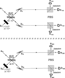
Figure 1: Circuit for the hyper-entangled Bell-like state analyzer where momentum DOF act as system qubits while polarisation DOF act as control qubits.

The action of the balanced beam splitter is given as:

$$\hat{a}^{{\dagger}}_{1}\ket{0}\longrightarrow\frac{(\hat{a}^{{\dagger}}_{1}+\hat{b}^{{\dagger}}_{1})}{\sqrt{2}}\ket{0}$$ (17)

$$\hat{b}^{{\dagger}}_{1}\ket{0}\longrightarrow\frac{(\hat{a}^{{\dagger}}_{1}-\hat{b}^{{\dagger}}_{1})}{\sqrt{2}}\ket{0}$$ (18)

Similarly, the action of an unbalanced beam splitter can be written as:

$$\hat{a}^{{\dagger}}_{2}\ket{0}\longrightarrow(\cos(\theta)\hat{a}^{{\dagger}}_{2}+\sin(\theta)\hat{b}^{{\dagger}}_{2})\ket{0}$$ (19)

$$\hat{b}^{{\dagger}}_{2}\ket{0}\longrightarrow(\sin(\theta)\hat{a}^{{\dagger}}_{2}-\cos(\theta)\hat{b}^{{\dagger}}_{2})\ket{0}$$ (20)

Finally, the action of PBS is mathematically represented as:

$$\hat{a}^{{\dagger}}_{1}\hat{h}^{{\dagger}}_{1}\ket{0}\longrightarrow\hat{a}^{{\dagger}}_{1H}\hat{h}^{{\dagger}}_{1}\ket{0}$$ (21)

$$\hat{a}^{{\dagger}}_{1}\hat{v}^{{\dagger}}_{1}\ket{0}\longrightarrow\hat{a}^{{\dagger}}_{1V}\hat{v}^{{\dagger}}_{1}\ket{0}$$ (22)

$$\hat{a}^{{\dagger}}_{2}\hat{h}^{{\dagger}}_{2}\ket{0}\longrightarrow\hat{a}^{{\dagger}}_{2H}\hat{h}^{{\dagger}}_{2}\ket{0}$$ (23)

$$\hat{a}^{{\dagger}}_{2}\hat{v}^{{\dagger}}_{2}\ket{0}\longrightarrow\hat{a}^{{\dagger}}_{2V}\hat{v}^{{\dagger}}_{2}\ket{0}$$ (24)

$$\hat{b}^{{\dagger}}_{1}\hat{h}^{{\dagger}}_{1}\ket{0}\longrightarrow\hat{b}^{{\dagger}}_{1H}\hat{h}^{{\dagger}}_{1}\ket{0}$$ (25)

$$\hat{b}^{{\dagger}}_{1}\hat{v}^{{\dagger}}_{1}\ket{0}\longrightarrow\hat{b}^{{\dagger}}_{1V}\hat{v}^{{\dagger}}_{1}\ket{0}$$ (26)

$$\hat{b}^{{\dagger}}_{2}\hat{h}^{{\dagger}}_{2}\ket{0}\longrightarrow\hat{b}^{{\dagger}}_{2H}\hat{h}^{{\dagger}}_{2}\ket{0}$$ (27)

$$\hat{b}^{{\dagger}}_{2}\hat{v}^{{\dagger}}_{2}\ket{0}\longrightarrow\hat{b}^{{\dagger}}_{2V}\hat{v}^{{\dagger}}_{2}\ket{0}$$ (28)

Being equipped with all the necessary transformations we can now analyze what will happen to the state in Eqn.(LABEL:Belllikehyperm) when they are passed through the circuit in Fig.1. We can easily verify that after passing through the circuit before entering the PBS for detection

$$|\Theta_{1}\rangle\longrightarrow\Big{(} \frac{1}{2}\hat{a}^{{\dagger}}_{1}\hat{a}^{{\dagger}}_{2}\hat{h}^{{\dagger}}_{1}\hat{v}^{{\dagger}}_{2}\sin\left(2\theta\right)+\frac{1}{2}\hat{a}^{{\dagger}}_{1}\hat{a}^{{\dagger}}_{2}\hat{h}^{{\dagger}}_{2}\hat{v}^{{\dagger}}_{1}\sin\left(2\theta\right)$$

$$-\frac{1}{2}\hat{a}^{{\dagger}}_{1}\hat{b}^{{\dagger}}_{2}\hat{h}^{{\dagger}}_{1}\hat{v}^{{\dagger}}_{2}\cos\left(2\theta\right)-\frac{1}{2}\hat{a}^{{\dagger}}_{1}\hat{b}^{{\dagger}}_{2}\hat{h}^{{\dagger}}_{2}\hat{v}^{{\dagger}}_{1}\cos\left(2\theta\right)$$

$$+\frac{1}{2}\hat{b}^{{\dagger}}_{1}\hat{b}^{{\dagger}}_{2}\hat{h}^{{\dagger}}_{1}\hat{v}^{{\dagger}}_{2}+\frac{1}{2}\hat{b}^{{\dagger}}_{1}\hat{b}^{{\dagger}}_{2}\hat{h}^{{\dagger}}_{2}\hat{v}^{{\dagger}}_{1}\Big{)}\ket{0}$$ (29)

$$|\Theta_{2}\rangle\longrightarrow\Big{(} \frac{1}{2}\hat{a}^{{\dagger}}_{1}\hat{a}^{{\dagger}}_{2}\hat{h}^{{\dagger}}_{1}\hat{v}^{{\dagger}}_{2}\cos\left(2\theta\right)+\frac{1}{2}\hat{a}^{{\dagger}}_{1}\hat{a}^{{\dagger}}_{2}\hat{h}^{{\dagger}}_{2}\hat{v}^{{\dagger}}_{1}\cos\left(2\theta\right)$$

$$+\frac{1}{2}\hat{a}^{{\dagger}}_{1}\hat{b}^{{\dagger}}_{2}\hat{h}^{{\dagger}}_{1}\hat{v}^{{\dagger}}_{2}\sin\left(2\theta\right)+\frac{1}{2}\hat{a}^{{\dagger}}_{1}\hat{b}^{{\dagger}}_{2}\hat{h}^{{\dagger}}_{2}\hat{v}^{{\dagger}}_{1}\sin\left(2\theta\right)$$

$$+\frac{1}{2}\hat{a}^{{\dagger}}_{2}\hat{b}^{{\dagger}}_{1}\hat{h}^{{\dagger}}_{1}\hat{v}^{{\dagger}}_{2}+\frac{1}{2}\hat{a}^{{\dagger}}_{2}\hat{b}^{{\dagger}}_{1}\hat{h}^{{\dagger}}_{2}\hat{v}^{{\dagger}}_{1}\Big{)}\ket{0}$$ (30)

$$|\Theta_{3}\rangle\longrightarrow\Big{(} \frac{1}{2}\hat{a}^{{\dagger}}_{1}\hat{a}^{{\dagger}}_{2}\hat{h}^{{\dagger}}_{1}\hat{h}^{{\dagger}}_{2}+\frac{1}{2}\hat{a}^{{\dagger}}_{1}\hat{a}^{{\dagger}}_{2}\hat{v}^{{\dagger}}_{1}\hat{v}^{{\dagger}}_{2}$$

$$-\frac{1}{2}\hat{a}^{{\dagger}}_{2}\hat{b}^{{\dagger}}_{1}\hat{h}^{{\dagger}}_{1}\hat{h}^{{\dagger}}_{2}\cos\left(2\theta\right)-\frac{1}{2}\hat{a}^{{\dagger}}_{2}\hat{b}^{{\dagger}}_{1}\hat{v}^{{\dagger}}_{1}\hat{v}^{{\dagger}}_{2}\cos\left(2\theta\right)$$

$$-\frac{1}{2}\hat{b}^{{\dagger}}_{1}\hat{b}^{{\dagger}}_{2}\hat{h}^{{\dagger}}_{1}\hat{h}^{{\dagger}}_{2}\sin\left(2\theta\right)-\frac{1}{2}\hat{b}^{{\dagger}}_{1}\hat{b}^{{\dagger}}_{2}\hat{v}^{{\dagger}}_{1}\hat{v}^{{\dagger}}_{2}\sin\left(2\theta\right)\Big{)}\ket{0}$$ (31)

$$|\Theta_{4}\rangle\longrightarrow\Big{(} -\frac{1}{2}\hat{a}^{{\dagger}}_{1}\hat{b}^{{\dagger}}_{2}\hat{h}^{{\dagger}}_{1}\hat{h}^{{\dagger}}_{2}-\frac{1}{2}\hat{a}^{{\dagger}}_{1}\hat{b}^{{\dagger}}_{2}\hat{v}^{{\dagger}}_{1}\hat{v}^{{\dagger}}_{2}$$

$$+\frac{1}{2}\hat{a}^{{\dagger}}_{2}\hat{b}^{{\dagger}}_{1}\hat{h}^{{\dagger}}_{1}\hat{h}^{{\dagger}}_{2}\sin\left(2\theta\right)+\frac{1}{2}\hat{a}^{{\dagger}}_{2}\hat{b}^{{\dagger}}_{1}\hat{v}^{{\dagger}}_{1}\hat{v}^{{\dagger}}_{2}\sin\left(2\theta\right)$$

$$-\frac{1}{2}\hat{b}^{{\dagger}}_{1}\hat{b}^{{\dagger}}_{2}\hat{h}^{{\dagger}}_{1}\hat{h}^{{\dagger}}_{2}\cos\left(2\theta\right)-\frac{1}{2}\hat{b}^{{\dagger}}_{1}\hat{b}^{{\dagger}}_{2}\hat{v}^{{\dagger}}_{1}\hat{v}^{{\dagger}}_{2}\cos\left(2\theta\right)\Big{)}\ket{0}$$ (32)

Photons in these states then pass through PBS and are detected by single photon detectors. We here make two observations:

• For states $|\Theta_{1}\rangle$ and $|\Theta_{2}\rangle$ both the photons are always detected in detectors oriented in directions perpendicular to each other. Furthermore,in this case, we have the following observation:

  1. The terms $\{\hat{b}^{{\dagger}}_{1}\hat{b}^{{\dagger}}_{2}\hat{h}^{{\dagger}}_{2}\hat{v}^{{\dagger}}_{1},\hat{b}^{{\dagger}}_{1}\hat{b}^{{\dagger}}_{2}\hat{h}^{{\dagger}}_{1}\hat{v}^{{\dagger}}_{2}\}$ are uniquely present in $|\Theta_{1}\rangle$. Thus clicking of detectors $\hat{b}^{{\dagger}}_{1V}$ and $\hat{b}^{{\dagger}}_{2H}$ or $\hat{b}^{{\dagger}}_{1H}$ and $\hat{b}^{{\dagger}}_{2V}$ indicates unambiguous detection of this state.

  2. The erms $\{\hat{b}^{{\dagger}}_{1}\hat{a}^{{\dagger}}_{2}\hat{h}^{{\dagger}}_{2}\hat{v}^{{\dagger}}_{1},\hat{b}^{{\dagger}}_{1}\hat{a}^{{\dagger}}_{2}\hat{h}^{{\dagger}}_{1}\hat{v}^{{\dagger}}_{2}\}$ are uniquely present in $|\Theta_{2}\rangle$. Thus clicking of detectors $\hat{b}^{{\dagger}}_{1V}$ and $\hat{a}^{{\dagger}}_{2H}$ or $\hat{b}^{{\dagger}}_{1H}$ and $\hat{a}^{{\dagger}}_{2V}$ indicates unambiguous detection of this state.

• For states $|\Theta_{3}\rangle$ and $|\Theta_{4}\rangle$ both the photons are always detected in detectors oriented in directions parallel to each other. Furthermore, we have, in this case, the following observation:

  1. Terms $\{\hat{a}^{{\dagger}}_{1}\hat{a}^{{\dagger}}_{2}\hat{h}^{{\dagger}}_{2}\hat{h}^{{\dagger}}_{1},\hat{a}^{{\dagger}}_{1}\hat{a}^{{\dagger}}_{2}\hat{v}^{{\dagger}}_{1}\hat{v}^{{\dagger}}_{2}\}$ are uniquely present in $|\Theta_{3}\rangle$. Thus clicking of detectors $\hat{a}^{{\dagger}}_{1H}$ and $\hat{a}^{{\dagger}}_{2H}$ or $\hat{a}^{{\dagger}}_{1V}$ and $\hat{a}^{{\dagger}}_{2V}$ indicates unambiguous detection of this state.

  2. Terms $\{\hat{a}^{{\dagger}}_{1}\hat{b}^{{\dagger}}_{2}\hat{h}^{{\dagger}}_{2}\hat{h}^{{\dagger}}_{1},\hat{a}^{{\dagger}}_{1}\hat{b}^{{\dagger}}_{2}\hat{v}^{{\dagger}}_{1}\hat{v}^{{\dagger}}_{2}\}$ are uniquely present in $|\Theta_{4}\rangle$. Thus clicking of detectors $\hat{a}^{{\dagger}}_{1H}$ and $\hat{b}^{{\dagger}}_{2H}$ or $\hat{a}^{{\dagger}}_{1V}$ and $\hat{b}^{{\dagger}}_{2V}$ indicates unambiguous detection of this state.

There will be detection events where some ambiguity will be there about which state is present. Thus success probability is necessarily not $100\%$. If we consider that all four states are provided to us with equal probability then the success probability is:

$$P_{succ} =\frac{1}{4}\Big{(}\frac{1}{4}+\frac{1}{4}\Big{)}+\frac{1}{4}\Big{(}\frac{1}{4}+\frac{1}{4}\Big{)}+\frac{1}{4}\Big{(}\frac{1}{4}+\frac{1}{4}\Big{)}+\frac{1}{4}\Big{(}\frac{1}{4}+\frac{1}{4}\Big{)}$$

$$=\frac{1}{2}$$ (33)

Thus success probability of unambiguous state discrimination is $50\%$. Comparing it with [24] we note that not only success probability is boosted from $25\%$, but also all four Bell-like states can be distinguished as there, only two of them at a time ($|\psi_{3}\rangle$ and $|\psi_{4}\rangle)$ or $(|\psi_{1}\rangle$ and $|\psi_{2}\rangle$) can be distinguished. Thus hyperentanglement acts as a resource in order to discriminate among them just like it happens in Bell state analysis(BSA) although success probability doesn’t reach $100\%$ as it reaches for Bell states. It is, of course, important to mention here that the optimal success probability in the case of unambiguous discrimination of the four Bell-like states (supplied with equal apriori probabilities) of two photons in their momenta degrees of freedom while the two photons are also maximally entangled in their polarization degrees of freedom – as given in Eqns. (5) - (8) – may turn out to be more than $50\%$.

III Ancillary entanglement in momentum degrees of freedom

We can also consider polarisation degrees of freedom as system qubits while momentum degrees of freedom serve as a source of ancillary entanglement. Similar to the previous section joint state of four Bell-like states in polarisation basis and ancillary qubits in the momentum basis can be written as

$$|\Xi_{1}\rangle=(\sin(\theta)\hat{h}^{{\dagger}}_{1}\hat{h}^{{\dagger}}_{2}+\cos(\theta)\hat{v}^{{\dagger}}_{1}\hat{v}^{{\dagger}}_{2})\otimes\frac{(\hat{a}^{{\dagger}}_{1}\hat{b}^{{\dagger}}_{2}+\hat{b}^{{\dagger}}_{1}\hat{a}^{{\dagger}}_{2})}{\sqrt{2}}\ket{0}$$ (34)

$$|\Xi_{2}\rangle=(\cos(\theta)\hat{h}^{{\dagger}}_{1}\hat{h}^{{\dagger}}_{2}-\sin(\theta)\hat{v}^{{\dagger}}_{1}\hat{v}^{{\dagger}}_{2})\otimes\frac{(\hat{a}^{{\dagger}}_{1}\hat{b}^{{\dagger}}_{2}+\hat{b}^{{\dagger}}_{1}\hat{a}^{{\dagger}}_{2})}{\sqrt{2}}\ket{0}$$ (35)

$$|\Xi_{3}\rangle=(\sin(\theta)\hat{h}^{{\dagger}}_{1}\hat{v}^{{\dagger}}_{2}+\cos(\theta)\hat{v}^{{\dagger}}_{1}\hat{h}^{{\dagger}}_{2})\otimes\frac{(\hat{a}^{{\dagger}}_{1}\hat{b}^{{\dagger}}_{2}+\hat{b}^{{\dagger}}_{1}\hat{a}^{{\dagger}}_{2})}{\sqrt{2}}\ket{0}$$ (36)

$$|\Xi_{4}\rangle=(\cos(\theta)\hat{h}^{{\dagger}}_{1}\hat{v}^{{\dagger}}_{2}-\sin(\theta)\hat{v}^{{\dagger}}_{1}\hat{h}^{{\dagger}}_{2})\otimes\frac{(\hat{a}^{{\dagger}}_{1}\hat{b}^{{\dagger}}_{2}+\hat{b}^{{\dagger}}_{1}\hat{a}^{{\dagger}}_{2})}{\sqrt{2}}\ket{0}$$ (37)

The circuit used for state discrimination is shown in Fig.2. Here first, photons pass through PBS which acts as a CNOT operation with polarisation DOF as the system qubit while momentum DOF as the control qubit. The transformation relations are given as:

$$\hat{h}^{{\dagger}}_{1}\hat{a}^{{\dagger}}_{1}\ket{0}\longrightarrow\hat{h}^{{\dagger}}_{1}\hat{a}^{{\dagger}}_{1}\ket{0}$$ (38)

$$\hat{h}^{{\dagger}}_{1}\hat{b}^{{\dagger}}_{1}\ket{0}\longrightarrow\hat{h}^{{\dagger}}_{1}\hat{b}^{{\dagger}}_{1}\ket{0}$$ (39)

$$\hat{h}^{{\dagger}}_{2}\hat{a}^{{\dagger}}_{2}\ket{0}\longrightarrow\hat{h}^{{\dagger}}_{2}\hat{a}^{{\dagger}}_{2}\ket{0}$$ (40)

$$\hat{h}^{{\dagger}}_{2}\hat{b}^{{\dagger}}_{2}\ket{0}\longrightarrow\hat{h}^{{\dagger}}_{2}\hat{b}^{{\dagger}}_{2}\ket{0}$$ (41)

$$\hat{v}^{{\dagger}}_{1}\hat{a}^{{\dagger}}_{1}\ket{0}\longrightarrow\hat{v}^{{\dagger}}_{1}\hat{b}^{{\dagger}}_{1}\ket{0}$$ (42)

$$\hat{v}^{{\dagger}}_{1}\hat{b}^{{\dagger}}_{1}\ket{0}\longrightarrow\hat{v}^{{\dagger}}_{1}\hat{a}^{{\dagger}}_{1}\ket{0}$$ (43)

$$\hat{v}^{{\dagger}}_{2}\hat{a}^{{\dagger}}_{2}\ket{0}\longrightarrow\hat{v}^{{\dagger}}_{2}\hat{b}^{{\dagger}}_{2}\ket{0}$$ (44)

$$\hat{v}^{{\dagger}}_{2}\hat{b}^{{\dagger}}_{2}\ket{0}\longrightarrow\hat{v}^{{\dagger}}_{2}\hat{a}^{{\dagger}}_{2}\ket{0}$$ (45)

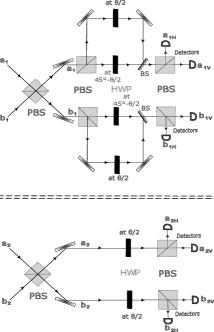
Figure 2: Circuit for the hyper-entangled Bell-like state analyzer where polarisation DOF act as system qubits while momentum DOF act as control qubits.

After that, another PBS is used in the circuit involving modes $\hat{a}^{{\dagger}}_{1}$ and $\hat{b}^{{\dagger}}_{1}$. It is used so that HWP mounted at angle $\frac{\theta}{2}$ acts on mode $\hat{h}^{{\dagger}}_{1}$ while HWP mounted at angle $45^{\circ}-\frac{\theta}{2}$ acts on mode $\hat{h}^{{\dagger}}_{2}$. This kind of asymmetry is necessary for certain cancellations which render Bell-like states unambiguously distinguishable. In the circuit involving modes $\hat{a}^{{\dagger}}_{2}$ and $\hat{b}^{{\dagger}}_{2}$ both are passed through HWP mounted at an angle $\frac{\theta}{2}$. The transformation rules for a modes $\hat{h}^{{\dagger}}_{2}$ and $\hat{v}^{{\dagger}}_{2}$are

$$\hat{h}^{{\dagger}}_{2}\ket{0}\longrightarrow(\cos(\theta)\hat{h}^{{\dagger}}_{2}+\sin(\theta)\hat{v}^{{\dagger}}_{2})\ket{0}$$ (46)

$$\hat{v}^{{\dagger}}_{2}\ket{0}\longrightarrow(\sin(\theta)\hat{h}^{{\dagger}}_{2}-\cos(\theta)\hat{v}^{{\dagger}}_{2})\ket{0}$$ (47)

While modes $\hat{h}^{{\dagger}}_{1}$ and $\hat{v}^{{\dagger}}_{1}$ transform as

$$\hat{h}^{{\dagger}}_{1}\ket{0}\longrightarrow(\cos(\theta)\hat{h}^{{\dagger}}_{1}+\sin(\theta)\hat{v}^{{\dagger}}_{1})\ket{0}$$ (48)

$$\hat{v}^{{\dagger}}_{1}\ket{0}\longrightarrow(\cos(\theta)\hat{h}^{{\dagger}}_{1}-\sin(\theta)\hat{v}^{{\dagger}}_{1})\ket{0}$$ (49)

A beam splitter is used to then merge the splitted modes $\hat{h}^{{\dagger}}_{1}$ and $\hat{v}^{{\dagger}}_{1}$ after HWPs act on them. The output is recorded from only one arm of the beam splitter resulting in the $50\%$ loss. It is worth mentioning that collecting output from either arm of the beam splitter is equivalent from the state discrimination point of view. After passing through the circuit the states from Eqn. (34)— (37) just before entering PBS are given as:

$$|\Xi_{1}\rangle\longrightarrow\Big{(} \frac{\hat{a}^{{\dagger}}_{1}\hat{b}^{{\dagger}}_{2}\hat{h}^{{\dagger}}_{1}\hat{h}^{{\dagger}}_{2}\sin\left(\theta\right)}{\sqrt{2}}+\frac{\hat{a}^{{\dagger}}_{1}\hat{b}^{{\dagger}}_{2}\hat{h}^{{\dagger}}_{1}\hat{h}^{{\dagger}}_{2}\sin\left(\theta\right)\cos\left(2\theta\right)}{\sqrt{2}}$$

$$-\frac{\hat{a}^{{\dagger}}_{1}\hat{b}^{{\dagger}}_{2}\hat{h}^{{\dagger}}_{1}\hat{v}^{{\dagger}}_{2}\cos\left(\theta\right)}{2\sqrt{2}}-\frac{\hat{a}^{{\dagger}}_{1}\hat{b}^{{\dagger}}_{2}\hat{h}^{{\dagger}}_{1}\hat{v}^{{\dagger}}_{2}\cos\left(3\theta\right)}{2\sqrt{2}}$$

$$+\frac{\hat{a}^{{\dagger}}_{1}\hat{b}^{{\dagger}}_{2}\hat{v}^{{\dagger}}_{1}\hat{v}^{{\dagger}}_{2}\sin\left(\theta\right)}{\sqrt{2}}+\frac{\hat{a}^{{\dagger}}_{2}\hat{b}^{{\dagger}}_{1}\hat{h}^{{\dagger}}_{1}\hat{h}^{{\dagger}}_{2}\sin\left(\theta\right)}{\sqrt{2}}$$

$$+\frac{\hat{a}^{{\dagger}}_{2}\hat{b}^{{\dagger}}_{1}\hat{h}^{{\dagger}}_{1}\hat{h}^{{\dagger}}_{2}\sin\left(\theta\right)\cos\left(2\theta\right)}{\sqrt{2}}-\frac{\hat{a}^{{\dagger}}_{2}\hat{b}^{{\dagger}}_{1}\hat{h}^{{\dagger}}_{1}\hat{v}^{{\dagger}}_{2}\cos\left(\theta\right)}{2\sqrt{2}}$$

$$-\frac{\hat{a}^{{\dagger}}_{2}\hat{b}^{{\dagger}}_{1}\hat{h}^{{\dagger}}_{1}\hat{v}^{{\dagger}}_{2}\cos\left(3\theta\right)}{2\sqrt{2}}+\frac{\hat{a}^{{\dagger}}_{2}\hat{b}^{{\dagger}}_{1}\hat{v}^{{\dagger}}_{1}\hat{v}^{{\dagger}}_{2}\sin\left(\theta\right)}{\sqrt{2}}\Big{)}\ket{0}$$ (50)

$$|\Xi_{2}\rangle\longrightarrow\Big{(} \frac{\hat{a}^{{\dagger}}_{1}\hat{b}^{{\dagger}}_{2}\hat{h}^{{\dagger}}_{1}\hat{h}^{{\dagger}}_{2}\cos\left(\theta\right)}{2\sqrt{2}}+\frac{\hat{a}^{{\dagger}}_{1}\hat{b}^{{\dagger}}_{2}\hat{h}^{{\dagger}}_{1}\hat{h}^{{\dagger}}_{2}\cos\left(3\theta\right)}{2\sqrt{2}}$$

$$+\frac{\hat{a}^{{\dagger}}_{1}\hat{b}^{{\dagger}}_{2}\hat{h}^{{\dagger}}_{1}\hat{v}^{{\dagger}}_{2}\sin\left(\theta\right)}{\sqrt{2}}+\frac{\hat{a}^{{\dagger}}_{1}\hat{b}^{{\dagger}}_{2}\hat{h}^{{\dagger}}_{1}\hat{v}^{{\dagger}}_{2}\sin\left(\theta\right)\cos\left(2\theta\right)}{\sqrt{2}}$$

$$+\frac{\hat{a}^{{\dagger}}_{1}\hat{b}^{{\dagger}}_{2}\hat{h}^{{\dagger}}_{2}\hat{v}^{{\dagger}}_{1}\sin\left(\theta\right)}{\sqrt{2}}+\frac{\hat{a}^{{\dagger}}_{2}\hat{b}^{{\dagger}}_{1}\hat{h}^{{\dagger}}_{1}\hat{h}^{{\dagger}}_{2}\cos\left(\theta\right)}{2\sqrt{2}}$$

$$+\frac{\hat{a}^{{\dagger}}_{2}\hat{b}^{{\dagger}}_{1}\hat{h}^{{\dagger}}_{1}\hat{h}^{{\dagger}}_{2}\cos\left(3\theta\right)}{2\sqrt{2}}+\frac{\hat{a}^{{\dagger}}_{2}\hat{b}^{{\dagger}}_{1}\hat{h}^{{\dagger}}_{1}\hat{v}^{{\dagger}}_{2}\sin\left(\theta\right)}{\sqrt{2}}$$

$$+\frac{\hat{a}^{{\dagger}}_{2}\hat{b}^{{\dagger}}_{1}\hat{h}^{{\dagger}}_{1}\hat{v}^{{\dagger}}_{2}\sin\left(\theta\right)\cos\left(2\theta\right)}{\sqrt{2}}+\frac{\hat{a}^{{\dagger}}_{2}\hat{b}^{{\dagger}}_{1}\hat{h}^{{\dagger}}_{2}\hat{v}^{{\dagger}}_{1}\sin\left(\theta\right)}{\sqrt{2}}\Big{)}\ket{0}$$ (51)

$$|\Xi_{3}\rangle\longrightarrow\Big{(} \frac{\hat{a}^{{\dagger}}_{1}\hat{a}^{{\dagger}}_{2}\hat{h}^{{\dagger}}_{1}\hat{h}^{{\dagger}}_{2}\cos\left(\theta\right)}{\sqrt{2}}+\frac{\hat{a}^{{\dagger}}_{1}\hat{a}^{{\dagger}}_{2}\hat{h}^{{\dagger}}_{2}\hat{v}^{{\dagger}}_{1}\sin\left(\theta\right)}{2\sqrt{2}}$$

$$-\frac{\hat{a}^{{\dagger}}_{1}\hat{a}^{{\dagger}}_{2}\hat{h}^{{\dagger}}_{2}\hat{v}^{{\dagger}}_{1}\sin\left(3\theta\right)}{2\sqrt{2}}-\frac{\hat{a}^{{\dagger}}_{1}\hat{a}^{{\dagger}}_{2}\hat{v}^{{\dagger}}_{1}\hat{v}^{{\dagger}}_{2}\cos\left(\theta_{1}\right)}{2\sqrt{2}}$$

$$+\frac{\hat{a}^{{\dagger}}_{1}\hat{a}^{{\dagger}}_{2}\hat{v}^{{\dagger}}_{1}\hat{v}^{{\dagger}}_{2}\cos\left(3\theta\right)}{2\sqrt{2}}+\frac{\hat{b}^{{\dagger}}_{1}\hat{b}^{{\dagger}}_{2}\hat{h}^{{\dagger}}_{1}\hat{h}^{{\dagger}}_{2}\cos\left(\theta\right)}{\sqrt{2}}$$

$$+\frac{\hat{b}^{{\dagger}}_{1}\hat{b}^{{\dagger}}_{2}\hat{h}^{{\dagger}}_{2}\hat{v}^{{\dagger}}_{1}\sin\left(\theta\right)}{2\sqrt{2}}-\frac{\hat{b}^{{\dagger}}_{1}\hat{b}^{{\dagger}}_{2}\hat{h}^{{\dagger}}_{2}\hat{v}^{{\dagger}}_{1}\sin\left(3\theta\right)}{2\sqrt{2}}$$

$$-\frac{\hat{b}^{{\dagger}}_{1}\hat{b}^{{\dagger}}_{2}\hat{v}^{{\dagger}}_{1}\hat{v}^{{\dagger}}_{2}\cos\left(\theta\right)}{2\sqrt{2}}+\frac{\hat{b}^{{\dagger}}_{1}\hat{b}^{{\dagger}}_{2}\hat{v}^{{\dagger}}_{1}\hat{v}^{{\dagger}}_{2}\cos\left(3\theta\right)}{2\sqrt{2}}\Big{)}\ket{0}$$ (52)

$$|\Xi_{4}\rangle\longrightarrow\Big{(} -\frac{\hat{a}^{{\dagger}}_{1}\hat{a}^{{\dagger}}_{2}\hat{h}^{{\dagger}}_{1}\hat{v}^{{\dagger}}_{2}\cos\left(\theta\right)}{\sqrt{2}}+\frac{\hat{a}^{{\dagger}}_{1}\hat{a}^{{\dagger}}_{2}\hat{h}^{{\dagger}}_{2}\hat{v}^{{\dagger}}_{1}\cos\left(\theta\right)}{2\sqrt{2}}$$

$$-\frac{\hat{a}^{{\dagger}}_{1}\hat{a}^{{\dagger}}_{2}\hat{h}^{{\dagger}}_{2}\hat{v}^{{\dagger}}_{1}\cos\left(3\theta\right)}{2\sqrt{2}}+\frac{\hat{a}^{{\dagger}}_{1}\hat{a}^{{\dagger}}_{2}\hat{v}^{{\dagger}}_{1}\hat{v}^{{\dagger}}_{2}\sin\left(\theta_{1}\right)}{2\sqrt{2}}$$

$$-\frac{\hat{a}^{{\dagger}}_{1}\hat{a}^{{\dagger}}_{2}\hat{v}^{{\dagger}}_{1}\hat{v}^{{\dagger}}_{2}\sin\left(3\theta\right)}{2\sqrt{2}}-\frac{\hat{b}^{{\dagger}}_{1}\hat{b}^{{\dagger}}_{2}\hat{h}^{{\dagger}}_{1}\hat{v}^{{\dagger}}_{2}\cos\left(\theta\right)}{\sqrt{2}}$$

$$+\frac{\hat{b}^{{\dagger}}_{1}\hat{b}^{{\dagger}}_{2}\hat{h}^{{\dagger}}_{2}\hat{v}^{{\dagger}}_{1}\cos\left(\theta\right)}{2\sqrt{2}}-\frac{\hat{b}^{{\dagger}}_{1}\hat{b}^{{\dagger}}_{2}\hat{h}^{{\dagger}}_{2}\hat{v}^{{\dagger}}_{1}\cos\left(3\theta\right)}{2\sqrt{2}}$$

$$+\frac{\hat{b}^{{\dagger}}_{1}\hat{b}^{{\dagger}}_{2}\hat{v}^{{\dagger}}_{1}\hat{v}^{{\dagger}}_{2}\sin\left(\theta\right)}{2\sqrt{2}}-\frac{\hat{b}^{{\dagger}}_{1}\hat{b}^{{\dagger}}_{2}\hat{v}^{{\dagger}}_{1}\hat{v}^{{\dagger}}_{2}\sin\left(3\theta\right)}{2\sqrt{2}}\Big{)}\ket{0}$$ (54)

We make the following observations

• For states $|\Xi_{1}\rangle$ and $|\Xi_{2}\rangle$ both the photons are always detected as coincidence detections in modes $\{\hat{a}^{{\dagger}}_{1},\hat{b}^{{\dagger}}_{2}\}$ or $\{\hat{b}^{{\dagger}}_{1},\hat{a}^{{\dagger}}_{2}\}$. Furthermore between them

  1. Terms $\{\hat{b}^{{\dagger}}_{1}\hat{a}^{{\dagger}}_{2}\hat{v}^{{\dagger}}_{2}\hat{v}^{{\dagger}}_{1},\hat{a}^{{\dagger}}_{1}\hat{b}^{{\dagger}}_{2}\hat{v}^{{\dagger}}_{1}\hat{v}^{{\dagger}}_{2}\}$ are uniquely present in $|\Xi_{1}\rangle$. Thus clicking of detectors $\hat{b}^{{\dagger}}_{1V}$ and $\hat{a}^{{\dagger}}_{2V}$ or $\hat{a}^{{\dagger}}_{1V}$ and $\hat{b}^{{\dagger}}_{2V}$ indicates unambiguous detection of this state.

  2. Terms $\{\hat{b}^{{\dagger}}_{1}\hat{a}^{{\dagger}}_{2}\hat{h}^{{\dagger}}_{2}\hat{v}^{{\dagger}}_{1},\hat{a}^{{\dagger}}_{1}\hat{b}^{{\dagger}}_{2}\hat{h}^{{\dagger}}_{1}\hat{v}^{{\dagger}}_{2}\}$ are uniquely present in $|\Xi_{2}\rangle$. Thus clicking of detectors $\hat{a}^{{\dagger}}_{1V}$ and $\hat{b}^{{\dagger}}_{2H}$ or $\hat{b}^{{\dagger}}_{1H}$ and $\hat{a}^{{\dagger}}_{2V}$ indicates unambiguous detection of this state.

• For states $|\Xi_{3}\rangle$ and $|\Xi_{4}\rangle$ both the photons are always detected as coincidence detections in modes $\{\hat{a}^{{\dagger}}_{1},\hat{a}^{{\dagger}}_{2}\}$ or $\{\hat{b}^{{\dagger}}_{1},\hat{b}^{{\dagger}}_{2}\}$.

  1. Terms $\{\hat{a}^{{\dagger}}_{1}\hat{a}^{{\dagger}}_{2}\hat{h}^{{\dagger}}_{2}\hat{h}^{{\dagger}}_{1},\hat{b}^{{\dagger}}_{1}\hat{b}^{{\dagger}}_{2}\hat{h}^{{\dagger}}_{1}\hat{h}^{{\dagger}}_{2}\}$ are uniquely present in $|\Xi_{3}\rangle$. Thus clicking of detectors $\hat{a}^{{\dagger}}_{1H}$ and $\hat{a}^{{\dagger}}_{2H}$ or $\hat{b}^{{\dagger}}_{1V}$ and $\hat{b}^{{\dagger}}_{2V}$ indicates unambiguous detection of this state.

  2. Terms $\{\hat{a}^{{\dagger}}_{1}\hat{a}^{{\dagger}}_{2}\hat{v}^{{\dagger}}_{2}\hat{h}^{{\dagger}}_{1},\hat{b}^{{\dagger}}_{1}\hat{b}^{{\dagger}}_{2}\hat{h}^{{\dagger}}_{1}\hat{v}^{{\dagger}}_{2}\}$ are uniquely present in $|\Xi_{4}\rangle$. Thus clicking of detectors $\hat{a}^{{\dagger}}_{1H}$ and $\hat{a}^{{\dagger}}_{2V}$ or $\hat{b}^{{\dagger}}_{1H}$ and $\hat{b}^{{\dagger}}_{2V}$ indicates unambiguous detection of this state.

Again there will be some detection that will render the discrimination of these states ambiguous. Thus the success probability again won’t be $100\%$. The success probability can be calculated in a similar way as the previous section. It comes out to be

$$P_{succ} =\frac{1}{4}(\frac{\sin^{2}(\theta)}{2}+\frac{\sin^{2}(\theta)}{2})+\frac{1}{4}(\frac{\sin^{2}(\theta)}{2}+\frac{\sin^{2}(\theta)}{2})$$

$$+\frac{1}{4}(\frac{\cos^{2}(\theta)}{2}+\frac{\cos^{2}(\theta)}{2})+\frac{1}{4}(\frac{\cos^{2}(\theta)}{2}+\frac{\cos^{2}(\theta)}{2})$$

$$=\frac{1}{2}$$ (55)

Thus, in this case, we see that the success probability of unambiguous state discrimination is again $50\%$.

IV Ancillary entanglement in OAM degrees of freedom

Till now we have discussed how momentum DOF act as system qubit while polarisation DOF acts as ancillary qubits to assist in the unambiguous discrimination of Bell-like states. But photons have orbital angular momentum (OAM) DOF also. They can act as maximally entangled ancillary qubits also while polarisation DOF bein the system qubits. Such a scheme has been adopted by Kwiat et.al. in [17] to implement super-dense coding. The circuit presented here is on the same lines. It is shown in Fig. (3)

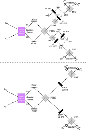
Figure 3: Circuit for the hyper-entangled Bell-like state analyzer where polarisation DOF act as system qubits while OAM DOF act as ancillary qubits.

The joint states of the system and ancillary qubits are given as:

$$|\Pi_{1}\rangle=(\sin(\theta)\hat{h}^{{\dagger}}_{1}\hat{h}^{{\dagger}}_{2}+\cos(\theta)\hat{v}^{{\dagger}}_{1}\hat{v}^{{\dagger}}_{2})\otimes\frac{(\hat{p}^{{\dagger}}_{1}\hat{m}^{{\dagger}}_{2}+\hat{m}^{{\dagger}}_{1}\hat{p}^{{\dagger}}_{2})}{\sqrt{2}}\ket{0}$$ (56)

$$|\Pi_{2}\rangle=(\cos(\theta)\hat{h}^{{\dagger}}_{1}\hat{h}^{{\dagger}}_{2}-\sin(\theta)\hat{v}^{{\dagger}}_{1}\hat{v}^{{\dagger}}_{2})\otimes\frac{(\hat{p}^{{\dagger}}_{1}\hat{m}^{{\dagger}}_{2}+\hat{m}^{{\dagger}}_{1}\hat{p}^{{\dagger}}_{2})}{\sqrt{2}}\ket{0}$$ (57)

$$|\Pi_{3}\rangle=(\sin(\theta)\hat{h}^{{\dagger}}_{1}\hat{v}^{{\dagger}}_{2}+\cos(\theta)\hat{v}^{{\dagger}}_{1}\hat{h}^{{\dagger}}_{2})\otimes\frac{(\hat{p}^{{\dagger}}_{1}\hat{m}^{{\dagger}}_{2}+\hat{m}^{{\dagger}}_{1}\hat{p}^{{\dagger}}_{2})}{\sqrt{2}}\ket{0}$$ (58)

$$|\Pi_{4}\rangle=(\cos(\theta)\hat{h}^{{\dagger}}_{1}\hat{v}^{{\dagger}}_{2}-\sin(\theta)\hat{v}^{{\dagger}}_{1}\hat{h}^{{\dagger}}_{2})\otimes\frac{(\hat{p}^{{\dagger}}_{1}\hat{m}^{{\dagger}}_{2}+\hat{m}^{{\dagger}}_{1}\hat{p}^{{\dagger}}_{2})}{\sqrt{2}}\ket{0}$$ (59)

where $\hat{p}^{{\dagger}}$ represent creation operator for OAM mode $+1$ while $\hat{m}^{{\dagger}}$ represent creation operator for OAM mode $-1$. Photons fall on a forked binary hologram and according to the OAM values $+1$ or $-1$ they will split into two beams marked by $(u_{1},d_{1})$ and $(u_{2},d_{2})$ for the first and second photon respectively. Then they pass through an assembly of PBSs and HWPs and are finally detected. To discriminate among Bell-like states it is necessary that HWPs act differently on both horizontally and vertically polarised first photon. Hence a PBS is used to split these two and then merge again by only recording output from one arm of a balanced beam splitter. This costs us a $50\%$ loss in the beam. The action of the forked binary hologram is given as:

$$\hat{h}^{{\dagger}}_{i}\hat{p}^{{\dagger}}_{i}\longrightarrow\hat{h}^{{\dagger}u_{i}}_{i}\hat{g}^{{\dagger}}_{i}$$

$$\hat{h}^{{\dagger}}_{i}\hat{m}^{{\dagger}}_{i}\longrightarrow\hat{h}^{{\dagger}d_{i}}_{i}\hat{g}^{{\dagger}}_{i}$$

$$\hat{v}^{{\dagger}}_{i}\hat{p}^{{\dagger}}_{i}\longrightarrow\hat{v}^{{\dagger}u_{i}}_{i}\hat{g}^{{\dagger}}_{i}$$

$$\hat{v}^{{\dagger}}_{i}\hat{m}^{{\dagger}}_{i}\longrightarrow\hat{v}^{{\dagger}d_{i}}_{i}\hat{g}^{{\dagger}}_{i}$$ (60)

where $\hat{g}^{{\dagger}}_{i}$ represent creation operator for $0$ OAM mode of ith particle. Thus the final states just before the final detection at PBS becomes

$$|\Pi_{1}\rangle\longrightarrow\Big{(} \frac{\hat{h}^{{\dagger}d_{1}}_{1}\hat{h}^{{\dagger}d_{2}}_{2}\cos\left(\theta\right)}{\sqrt{2}}+\frac{\hat{h}^{{\dagger}u_{1}}_{1}\hat{h}^{{\dagger}u_{2}}_{2}\cos\left(\theta\right)}{\sqrt{2}}$$

$$+\frac{\hat{h}^{{\dagger}d_{2}}_{2}\hat{v}^{{\dagger}d_{1}}_{1}\sin\left(\theta\right)}{2\sqrt{2}}-\frac{\hat{h}^{{\dagger}d_{2}}_{2}\hat{v}^{{\dagger}d_{1}}_{1}\sin\left(3\theta\right)}{2\sqrt{2}}$$

$$+\frac{\hat{h}^{{\dagger}u_{2}}_{2}\hat{v}^{{\dagger}u_{1}}_{1}\sin\left(\theta\right)}{2\sqrt{2}}-\frac{\hat{h}^{{\dagger}u_{2}}_{2}\hat{v}^{{\dagger}u_{1}}_{1}\sin\left(3\theta\right)}{2\sqrt{2}}$$

$$-\frac{\hat{v}^{{\dagger}d_{1}}_{1}\hat{v}^{{\dagger}d_{2}}_{2}\cos\left(\theta\right)}{2\sqrt{2}}+\frac{\hat{v}^{{\dagger}d_{1}}_{1}\hat{v}^{{\dagger}d_{2}}_{2}\cos\left(3\theta\right)}{2\sqrt{2}}$$

$$-\frac{\hat{v}^{{\dagger}u_{1}}_{1}\hat{v}^{{\dagger}u_{2}}_{2}\cos\left(\theta\right)}{2\sqrt{2}}+\frac{\hat{v}^{{\dagger}u_{1}}_{1}\hat{v}^{{\dagger}u_{2}}_{2}\cos\left(3\theta\right)}{2\sqrt{2}}\Big{)}\otimes\hat{g}^{{\dagger}}_{1}\hat{g}^{{\dagger}}_{2}\ket{0}$$ (61)

$$|\Pi_{2}\rangle\longrightarrow\Big{(} -\frac{\hat{h}^{{\dagger}d_{1}}_{1}\hat{v}^{{\dagger}d_{2}}_{2}\cos\left(\theta\right)}{\sqrt{2}}-\frac{\hat{h}^{{\dagger}u_{1}}_{1}\hat{v}^{{\dagger}u_{2}}_{2}\cos\left(\theta\right)}{\sqrt{2}}$$

$$+\frac{\hat{h}^{{\dagger}d_{2}}_{2}\hat{v}^{{\dagger}d_{1}}_{1}\cos\left(\theta\right)}{2\sqrt{2}}-\frac{\hat{h}^{{\dagger}d_{2}}_{2}\hat{v}^{{\dagger}d_{1}}_{1}\cos\left(3\theta\right)}{2\sqrt{2}}$$

$$+\frac{\hat{h}^{{\dagger}u_{2}}_{2}\hat{v}^{{\dagger}u_{1}}_{1}\cos\left(\theta\right)}{2\sqrt{2}}-\frac{\hat{h}^{{\dagger}u_{2}}_{2}\hat{v}^{{\dagger}u_{1}}_{1}\cos\left(3\theta\right)}{2\sqrt{2}}$$

$$+\frac{\hat{v}^{{\dagger}d_{1}}_{1}\hat{v}^{{\dagger}d_{2}}_{2}\sin\left(\theta\right)}{2\sqrt{2}}-\frac{\hat{v}^{{\dagger}d_{1}}_{1}\hat{v}^{{\dagger}d_{2}}_{2}\sin\left(3\theta\right)}{2\sqrt{2}}$$

$$+\frac{\hat{v}^{{\dagger}u_{1}}_{1}\hat{v}^{{\dagger}u_{2}}_{2}\sin\left(\theta\right)}{2\sqrt{2}}-\frac{\hat{v}^{{\dagger}u_{1}}_{1}\hat{v}^{{\dagger}u_{2}}_{2}\sin\left(3\theta\right)}{2\sqrt{2}}\Big{)}\otimes\hat{g}^{{\dagger}}_{1}\hat{g}^{{\dagger}}_{2}\ket{0}$$ (62)

$$|\Pi_{3}\rangle\longrightarrow\Big{(} \frac{\hat{h}^{{\dagger}d_{1}}_{1}\hat{h}^{{\dagger}u_{2}}_{2}\sin\left(\theta\right)}{\sqrt{2}}+\frac{\hat{h}^{{\dagger}d_{1}}_{1}\hat{h}^{{\dagger}u_{2}}_{2}\sin\left(\theta\right)\cos\left(2\theta_{1}\right)}{\sqrt{2}}$$

$$-\frac{\hat{h}^{{\dagger}d_{1}}_{1}\hat{v}^{{\dagger}u_{2}}_{2}\cos\left(\theta\right)}{2\sqrt{2}}-\frac{\hat{h}^{{\dagger}d_{1}}_{1}\hat{v}^{{\dagger}u_{2}}_{2}\cos\left(3\theta\right)}{2\sqrt{2}}$$

$$+\frac{\hat{h}^{{\dagger}u_{1}}_{1}\hat{h}^{{\dagger}d_{2}}_{2}\sin\left(\theta\right)}{\sqrt{2}}+\frac{\hat{h}^{{\dagger}u_{1}}_{1}\hat{h}^{{\dagger}d_{2}}_{2}\sin\left(\theta\right)\cos\left(2\theta_{1}\right)}{\sqrt{2}}$$

$$-\frac{\hat{h}^{{\dagger}u_{1}}_{1}\hat{v}^{{\dagger}d_{2}}_{2}\cos\left(\theta\right)}{2\sqrt{2}}-\frac{\hat{h}^{{\dagger}u_{1}}_{1}\hat{v}^{{\dagger}d_{2}}_{2}\cos\left(3\theta\right)}{2\sqrt{2}}$$

$$+\frac{\hat{v}^{{\dagger}d_{1}}_{1}\hat{v}^{{\dagger}u_{2}}_{2}\sin\left(\theta\right)}{\sqrt{2}}+\frac{\hat{v}^{{\dagger}u_{1}}_{1}\hat{v}^{{\dagger}d_{2}}_{2}\sin\left(\theta\right)}{\sqrt{2}}\Big{)}\otimes\hat{g}^{{\dagger}}_{1}\hat{g}^{{\dagger}}_{2}\ket{0}$$ (64)

$$|\Pi_{4}\rangle\longrightarrow\Big{(} \frac{\hat{h}^{{\dagger}d_{1}}_{1}\hat{h}^{{\dagger}u_{2}}_{2}\cos\left(\theta\right)}{2\sqrt{2}}+\frac{\hat{h}^{{\dagger}d_{1}}_{1}\hat{h}^{{\dagger}u_{2}}_{2}\cos\left(3\theta\right)}{2\sqrt{2}}$$

$$+\frac{\hat{h}^{{\dagger}d_{1}}_{1}\hat{v}^{{\dagger}u_{2}}_{2}\sin\left(\theta\right)}{2\sqrt{2}}+\frac{\hat{h}^{{\dagger}d_{1}}_{1}\hat{v}^{{\dagger}u_{2}}_{2}\sin\left(3\theta\right)}{2\sqrt{2}}$$

$$+\frac{\hat{h}^{{\dagger}u_{1}}_{1}\hat{h}^{{\dagger}d_{2}}_{2}\cos\left(\theta_{1}\right)}{2\sqrt{2}}+\frac{\hat{h}^{{\dagger}u_{1}}_{1}\hat{h}^{{\dagger}d_{2}}_{2}\cos\left(3\theta\right)}{2\sqrt{2}}$$

$$+\frac{\hat{h}^{{\dagger}u_{1}}_{1}\hat{v}^{{\dagger}d_{2}}_{2}\sin\left(\theta\right)}{2\sqrt{2}}+\frac{\hat{h}^{{\dagger}u_{1}}_{1}\hat{v}^{{\dagger}d_{2}}_{2}\sin\left(3\theta\right)}{2\sqrt{2}}$$

$$+\frac{\hat{h}^{{\dagger}d_{2}}_{2}\hat{v}^{{\dagger}u_{1}}_{1}\sin\left(\theta\right)}{\sqrt{2}}+\frac{\hat{h}^{{\dagger}u_{2}}_{2}\hat{v}^{{\dagger}d_{1}}_{1}\sin\left(\theta\right)}{\sqrt{2}}\Big{)}\otimes\hat{g}^{{\dagger}}_{1}\hat{g}^{{\dagger}}_{2}\ket{0}$$ (65)

We make the following observations

• For states $|\Pi_{1}\rangle$ and $|\Pi_{2}\rangle$ both the photons are always detected as coincidence detections in either path $(u_{1},u_{2})$ or paths $(d_{1},d_{2})$. Furthermore between them

  1. Terms $\{\hat{h}^{{\dagger}u_{1}}_{1}\hat{h}^{{\dagger}u_{2}}_{2},\hat{h}^{{\dagger}d_{1}}_{1}\hat{h}^{{\dagger}d_{2}}_{2}\}$ are uniquely present in $|\Pi_{1}\rangle$. Thus both the photons being horizontally polarised in paths $u_{1}(d_{1})$ and $u_{2}(d_{2})$ indicates unambiguous detection of this state.

  2. Terms $\{\hat{h}^{{\dagger}u_{1}}_{1}\hat{v}^{{\dagger}u_{2}}_{2},\hat{h}^{{\dagger}d_{1}}_{1}\hat{v}^{{\dagger}d_{2}}_{2}\}$ are uniquely present in $|\Pi_{2}\rangle$. Thus horizontally polarised first photon in paths $u_{1}(d_{1})$ and vertically polarised second photon in paths $u_{2}(d_{2})$ indicates unambiguous detection of this state.

• For states $|\Pi_{3}\rangle$ and $|\Pi_{4}\rangle$ both the photons are always simultaneously detected in both the paths u and d. Furthermore

  1. Terms $\{\hat{v}^{{\dagger}u_{1}}_{1}\hat{v}^{{\dagger}d_{2}}_{2},\hat{v}^{{\dagger}d_{1}}_{1}\hat{v}^{{\dagger}u_{2}}_{2}\}$ are uniquely present in $|\Pi_{3}\rangle$. Thus both the photons being vertically polarised in paths $u_{1}(d_{1})$ and $d_{2}(u_{2})$ indicates unambiguous detection of this state.

  2. Terms $\{\hat{v}^{{\dagger}u_{1}}_{1}\hat{h}^{{\dagger}d_{2}}_{2},\hat{v}^{{\dagger}d_{1}}_{1}\hat{h}^{{\dagger}u_{2}}_{2}\}$ are uniquely present in $|\Pi_{4}\rangle$. Thus vertically polarised first photon in paths $u_{1}(d_{1})$ and horizontally polarised second photon in paths $d_{2}(u_{2})$ indicates unambiguous detection of this state.

There will also be some detection events that will render the discrimination of the Bell-like states ambiguous. Thus success probability, unlike Bell state discrimination, will not be $100\%$. If all Bell-like states are provided with equal probability then success probability can be calculated as

$$P_{succ} =\frac{1}{4}(\frac{\sin^{2}(\theta)}{2}+\frac{\sin^{2}(\theta)}{2})+\frac{1}{4}(\frac{\sin^{2}(\theta)}{2}+\frac{\sin^{2}(\theta)}{2})$$

$$+\frac{1}{4}(\frac{\cos^{2}(\theta)}{2}+\frac{\cos^{2}(\theta)}{2})+\frac{1}{4}(\frac{\cos^{2}(\theta)}{2}+\frac{\cos^{2}(\theta)}{2})$$

$$=\frac{1}{2}$$ (66)

Thus success probability of unambiguous discrimination is essentially $50\%$. We would again like to stress the point that the aforesaid protocol may not be the optimal one.

V Using correlation in time DOF for Bell-like state analysis

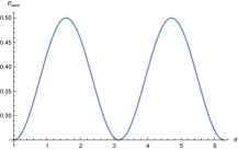
Figure 5: Variation of the success probability of state discrimination w.r.t. the state parameter $\theta$.

It is well known that the photon pair coming out of a spontaneous down conversion source is strongly correlated in time. This correlation can be used to distinguish Bell-like states. It was first proposed by Kwiat and Weinfurter [26] for Bell state analysis. The circuit is shown in Fig.(5)

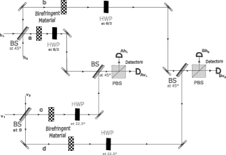
Figure 4: This is the circuit for a Bell-like state analyzer where correlation in time DOF of photon pair is used.

An entangled photon pair is generated by passing a pump photon beam through non-linear crystals where it undergoes the SPDC process. Horizontally polarised photons are passed through a balanced beam splitter while vertically polarised photons are passed through an unbalanced beam splitter. The output of both beam splitters is then passed through birefringent crystals. These crystals introduce the delay in the passing photon depending on their polarization. Horizontally polarised photon picks up a delay of, say, time $t_{h}$ while the vertically polarised photon is delayed by time $t_{v}$. Mathematically it can be written as:

$$\hat{h}^{{\dagger}}_{1}\longrightarrow\hat{h}^{{\dagger}}_{1}(t_{h})$$

$$\hat{h}^{{\dagger}}_{2}\longrightarrow\hat{h}^{{\dagger}}_{2}(t_{h})$$

$$\hat{v}^{{\dagger}}_{1}\longrightarrow\hat{v}^{{\dagger}}_{1}(t_{v})$$

$$\hat{v}^{{\dagger}}_{2}\longrightarrow\hat{v}^{{\dagger}}_{2}(t_{v})$$ (67)

The amount of delay depends on the length of the crystal. We have to bear two things in mind while introducing this delay:

• Both the delay times $t_{h}$ and $t_{v}$ should be greater than the coherence time of the entangled photon pair. This ensures that both the photons (horizontally and vertically polarised) can be distinguished by their arrival times $t_{h}$ and $t_{v}$ at the detectors.

• Both of these delay times should be less than the coherence time of the pump photon. this ensures that the photon pair as a whole cannot be distinguished by their times of creation i.e. terms like $\hat{x}^{{\dagger}}_{1}(t_{h})\hat{x}^{{\dagger}}_{2}(t_{h})$ and $\hat{x}^{{\dagger}}_{1}(t_{v})\hat{x}^{{\dagger}}_{2}(t_{v})$ are indistinguishable from each other hence will be replaced by $\hat{x}^{{\dagger}}_{1}\hat{x}^{{\dagger}}_{2}$ where $\hat{x}^{{\dagger}}\in\{\hat{h}^{{\dagger}},\hat{v}^{{\dagger}}\}$.

The horizontally polarised photons then pass through an HWP aligned at an angle $\frac{\theta}{2}$ while vertically polarised photons are passed through an HWP aligned at the angle of $22.5^{\circ}$. After merging two photons at the beam splitter the Bell-like states transform as

$$|\psi_{1}\rangle= (\sin(\theta)\hat{h}^{{\dagger}}_{1}\hat{v}^{{\dagger}}_{2}+\cos(\theta)\hat{v}^{{\dagger}}_{1}\hat{h}^{{\dagger}}_{2})\ket{0}$$

$$\longrightarrow \Big{(}\frac{\cos(\theta)}{2}\hat{h}^{{\dagger}}_{1}(t_{h})\hat{h}^{{\dagger}}_{1}(t_{v})-\frac{\cos(\theta)}{2}\hat{h}^{{\dagger}}_{1}(t_{h})\hat{v}^{{\dagger}}_{1}(t_{v})$$

$$+\frac{\sin(\theta)}{2}\hat{v}^{{\dagger}}_{1}(t_{h})\hat{h}^{{\dagger}}_{1}(t_{v})-\frac{\sin(\theta)}{2}\hat{v}^{{\dagger}}_{1}(t_{h})\hat{v}^{{\dagger}}_{1}(t_{v})$$

$$-\frac{\cos(\theta)\cos(2\theta)}{2}\hat{h}^{{\dagger}}_{2}(t_{h})\hat{h}^{{\dagger}}_{1}(t_{v})+\frac{\cos(\theta)\cos(2\theta)}{2}\hat{h}^{{\dagger}}_{2}(t_{h})\hat{v}^{{\dagger}}_{1}(t_{v})$$

$$-\frac{\sin(\theta)\cos(2\theta)}{2}\hat{v}^{{\dagger}}_{2}(t_{h})\hat{h}^{{\dagger}}_{1}(t_{v})+\frac{\sin(\theta)\cos(2\theta)}{2}\hat{v}^{{\dagger}}_{2}(t_{h})\hat{v}^{{\dagger}}_{1}(t_{v})$$

$$-\cos^{2}(\theta)\sin(\theta)\hat{h}^{{\dagger}}_{2}(t_{h})\hat{h}^{{\dagger}}_{2}(t_{v})+\cos^{2}(\theta)\sin(\theta)\hat{h}^{{\dagger}}_{2}(t_{h})\hat{v}^{{\dagger}}_{2}(t_{v})$$

$$-\sin^{2}(\theta)\cos(\theta)\hat{v}^{{\dagger}}_{2}(t_{h})\hat{h}^{{\dagger}}_{2}(t_{v})+\sin^{2}(\theta)\cos(\theta)\hat{v}^{{\dagger}}_{2}(t_{h})\hat{v}^{{\dagger}}_{2}(t_{v})\Big{)}\ket{0}$$ (68)

$$|\psi_{2}\rangle= (\cos(\theta)\hat{h}^{{\dagger}}_{1}\hat{v}^{{\dagger}}_{2}-\sin(\theta)\hat{v}^{{\dagger}}_{1}\hat{h}^{{\dagger}}_{2})\ket{0}$$

$$\longrightarrow -\Big{(}\frac{\cos(\theta)}{2}\hat{h}^{{\dagger}}_{1}(t_{h})\hat{h}^{{\dagger}}_{2}(t_{v})+\frac{\cos(\theta)}{2}\hat{h}^{{\dagger}}_{1}(t_{h})\hat{v}^{{\dagger}}_{2}(t_{v})$$

$$-\frac{\sin(\theta)}{2}\hat{v}^{{\dagger}}_{1}(t_{h})\hat{h}^{{\dagger}}_{2}(t_{v})+\frac{\sin(\theta)}{2}\hat{v}^{{\dagger}}_{1}(t_{h})\hat{v}^{{\dagger}}_{2}(t_{v})$$

$$-\frac{\cos(\theta)\cos(2\theta)}{2}\hat{h}^{{\dagger}}_{2}(t_{h})\hat{h}^{{\dagger}}_{2}(t_{v})+\frac{\cos(\theta)\cos(2\theta)}{2}\hat{h}^{{\dagger}}_{2}(t_{h})\hat{v}^{{\dagger}}_{2}(t_{v})$$

$$-\frac{\sin(\theta)\cos(2\theta)}{2}\hat{v}^{{\dagger}}_{2}(t_{h})\hat{h}^{{\dagger}}_{2}(t_{v})+\frac{\sin(\theta)\cos(2\theta)}{2}\hat{v}^{{\dagger}}_{2}(t_{h})\hat{v}^{{\dagger}}_{2}(t_{v})$$

$$+\cos^{2}(\theta)\sin(\theta)\hat{h}^{{\dagger}}_{2}(t_{h})\hat{h}^{{\dagger}}_{1}(t_{v})-\cos^{2}(\theta)\sin(\theta)\hat{h}^{{\dagger}}_{2}(t_{h})\hat{v}^{{\dagger}}_{1}(t_{v})$$

$$+\sin^{2}(\theta)\cos(\theta)\hat{v}^{{\dagger}}_{2}(t_{h})\hat{h}^{{\dagger}}_{1}(t_{v})-\sin^{2}(\theta)\cos(\theta)\hat{v}^{{\dagger}}_{2}(t_{h})\hat{v}^{{\dagger}}_{1}(t_{v})\Big{)}\ket{0}$$ (69)

$$|\psi_{3}\rangle= (\sin(\theta)\hat{h}^{{\dagger}}_{1}\hat{h}^{{\dagger}}_{2}+\cos(\theta)\hat{v}^{{\dagger}}_{1}\hat{v}^{{\dagger}}_{2})\ket{0}$$

$$\longrightarrow \Big{(}\sin(\theta)\cos^{2}(\theta))\hat{h}^{{\dagger}2}_{1}-\sin(\theta)\cos^{2}(\theta))\hat{h}^{{\dagger}2}_{2}+\frac{\sin(\theta)}{2}\hat{v}^{{\dagger}2}_{1}$$

$$-\frac{\sin(\theta)}{2}\hat{v}^{{\dagger}2}_{2}+\big{(}\sin^{2}(\theta)\cos(\theta)-\cos^{2}(\theta)\sin(\theta)\big{)}\hat{h}^{{\dagger}}_{1}\hat{v}^{{\dagger}}_{1}$$

$$-\big{(}\sin^{2}(\theta)\cos(\theta)-\cos^{2}(\theta)\sin(\theta)\big{)}\hat{h}^{{\dagger}}_{2}\hat{v}^{{\dagger}}_{2}$$

$$-\frac{\cos(\theta)\cos(2\theta)}{2}\hat{h}^{{\dagger}}_{1}\hat{h}^{{\dagger}}_{2}+\frac{\cos(\theta)\cos(2\theta)}{2}\hat{h}^{{\dagger}}_{1}\hat{v}^{{\dagger}}_{2}$$

$$+\frac{\cos(\theta)\cos(2\theta)}{2}\hat{v}^{{\dagger}}_{1}\hat{h}^{{\dagger}}_{2}-\frac{\cos(\theta)\cos(2\theta)}{2}\hat{v}^{{\dagger}}_{1}\hat{v}^{{\dagger}}_{2}\Big{)}\ket{0}$$ (71)

$$|\psi_{4}\rangle= (\cos(\theta)\hat{h}^{{\dagger}}_{1}\hat{h}^{{\dagger}}_{2}-\sin(\theta)\hat{v}^{{\dagger}}_{1}\hat{v}^{{\dagger}}_{2})\ket{0}$$

$$\longrightarrow \Big{(}\frac{\cos(\theta)\cos(2\theta)}{2}\hat{h}^{{\dagger}2}_{1}-\frac{\cos(\theta)\cos(2\theta)}{2}\hat{h}^{{\dagger}2}_{2}$$

$$+\big{(}\sin^{2}(\theta)\cos(\theta)+\cos^{2}(\theta)\sin(\theta)\big{)}\hat{h}^{{\dagger}}_{1}\hat{v}^{{\dagger}}_{1}$$

$$-\big{(}\sin^{2}(\theta)\cos(\theta)+\cos^{2}(\theta)\sin(\theta)\big{)}\hat{h}^{{\dagger}}_{2}\hat{v}^{{\dagger}}_{2}$$

$$+\frac{\sin(\theta)\cos(2\theta)}{2}\hat{h}^{{\dagger}}_{1}\hat{h}^{{\dagger}}_{2}-\frac{\sin(\theta)\cos(2\theta)}{2}\hat{h}^{{\dagger}}_{1}\hat{v}^{{\dagger}}_{2}$$

$$-\frac{\sin(\theta)\cos(2\theta)}{2}\hat{v}^{{\dagger}}_{1}\hat{h}^{{\dagger}}_{2}+\frac{\sin(\theta)\cos(2\theta)}{2}\hat{v}^{{\dagger}}_{1}\hat{v}^{{\dagger}}_{2}\Big{)}\ket{0}$$ (72)

We make the following observations:

1. Terms $\{\hat{h}^{{\dagger}}_{1}(t_{h})\hat{h}^{{\dagger}}_{1}(t_{v}),\hat{h}^{{\dagger}}_{1}(t_{h})\hat{v}^{{\dagger}}_{1}(t_{v}),\hat{v}^{{\dagger}}_{1}(t_{h})\hat{h}^{{\dagger}}_{1}(t_{v}),\hat{v}^{{\dagger}}_{1}(t_{h})\hat{v}^{{\dagger}}_{1}(t_{v})\}$ are uniquely present in $|\psi_{1}\rangle$. Thus detection of both the photon in detector $A(Ah_{1},Av_{1})$ with the delay of $|t_{h}-t_{v}|$ between them indicates the presence of this state.

2. Terms $\{\hat{h}^{{\dagger}}_{1}(t_{h})\hat{h}^{{\dagger}}_{2}(t_{v}),\hat{h}^{{\dagger}}_{1}(t_{h})\hat{v}^{{\dagger}}_{2}(t_{v}),\hat{v}^{{\dagger}}_{1}(t_{h})\hat{h}^{{\dagger}}_{2}(t_{v}),\hat{v}^{{\dagger}}_{1}(t_{h})\hat{v}^{{\dagger}}_{2}(t_{v})\}$ are uniquely present in $|\psi_{2}\rangle$.Thus detection of the first photon in detector $A(Ah_{1},Av_{1})$ and the second photon in detector $B(Bh_{2},Bv_{2})$ with the delay of $|t_{h}-t_{v}|$ between them indicates the presence of this state.

3. Terms $\hat{v}^{{\dagger}2}_{1},\hat{v}^{{\dagger}2}_{2}$ are uniquely present in $|\psi_{3}\rangle$. Thus if both photons are detected simultaneously without any delay in any of the detectors $Av_{1},Bv_{2}$ the presence of this state is confirmed.

Evidently, the present scheme does not provide an unambiguous discrimination of all the four Bell-Like states. In particular, if $\hat{h}^{{\dagger}2}_{1}$ or $\hat{h}^{{\dagger}2}_{2}$ clicks, it can happen for both $|{\psi}3\rangle$ as well as $|\psi_{4}\rangle$.

The success probability is necessarily not $100\%$. If we consider that all four states are provided to us with equal probability then the success probability is:

$$P_{succ} =\frac{1}{4}\Big{(}\frac{\sin^{2}(\theta)}{4}+\frac{\sin^{2}(\theta)}{4}+\frac{\cos^{2}(\theta)}{4}+\frac{\cos^{2}(\theta)}{4}\Big{)}$$

$$+\frac{1}{4}\Big{(}\frac{\sin^{2}(\theta)}{4}+\frac{\sin^{2}(\theta)}{4}+\frac{\cos^{2}(\theta)}{4}+\frac{\cos^{2}(\theta)}{4}\Big{)}$$

$$+\frac{1}{4}\Big{(}\frac{\sin^{2}(\theta)}{2}+\frac{\sin^{2}(\theta)}{2}\Big{)}+\frac{1}{4}(0)$$

$$=\frac{(1+\sin^{2}(\theta))}{4}$$ (73)

Interestingly success probability depends on the state parameter $\theta$ of the given Bell-like states which we want to discriminate. The expression success probability in Eqn. (V) is valid for $\theta\neq\frac{\pi}{4}$ and $0<\theta<\frac{\pi}{2}$.

Thus we observe that in case correlations in time are used to assist in the discrimination of four bell-like states the success probability although higher than $25\%$ unlike previous cases never reaches $50\%$ let alone $100\%$. Another interesting observation is that here, even ambiguously, we can only discriminate among three Bell-like states $\psi_{1},\psi_{2}$ and $\psi_{3}$. The state $\psi_{4}$ doesn’t have a unique detection signature. This is in stark contrast to Bell-state discrimination where we can discriminate among all 4 Bell states with $100\%$ success probability.

VI Bell-like state analysis using Ancillary qubits

Aside from using hyperentanglement extra ancillary photons can come to our aid for Bell-like state analysis. Grice found out that by using two ancillary maximally entangled photons [19] the success probability for Bell state discrimination can be enhanced to $75\%$ from $50\%$. Only two bell states ($\psi^{+}$ and $\psi^{-}$) are distinguishable without using any resource in a linear optical setting. The introduction of ancillary entangled qubits renders the remaining two ($\phi^{+}$ and $\phi^{-}$) also distinguishable (not unambiguously as there will be some detection signatures that will be common for both states). Thus success probability of Bell state discrimination increases from $50\%$ (two states are distinguishable without any ambiguity) to $75\%$ (all four can be distinguished with some ambiguity in ($\phi^{+}$ and $\phi^{-}$) ). We try to do a similar kind of thing here. The Bell-like states with ancillary photons are given as

$$|\Gamma_{1}\rangle= \left(\hat{a}^{{\dagger}}_{1}\hat{a}^{{\dagger}}_{4}\sin\left(\theta_{2}\right)+\hat{a}^{{\dagger}}_{2}\hat{a}^{{\dagger}}_{3}\cos\left(\theta_{2}\right)\right)$$

$$\qquad\qquad\qquad\otimes\left(\hat{a}^{{\dagger}}_{5}\hat{a}^{{\dagger}}_{7}\sin\left(\theta_{1}\right)+\hat{a}^{{\dagger}}_{6}\hat{a}^{{\dagger}}_{8}\cos\left(\theta_{1}\right)\right)\ket{0}$$ (74)

$$|\Gamma_{2}\rangle= \left(\hat{a}^{{\dagger}}_{1}\hat{a}^{{\dagger}}_{4}\cos\left(\theta_{2}\right)-\hat{a}^{{\dagger}}_{2}\hat{a}^{{\dagger}}_{3}\sin\left(\theta_{2}\right)\right)$$

$$\qquad\qquad\qquad\otimes\left(\hat{a}^{{\dagger}}_{5}\hat{a}^{{\dagger}}_{7}\sin\left(\theta_{1}\right)+\hat{a}^{{\dagger}}_{6}\hat{a}^{{\dagger}}_{8}\cos\left(\theta_{1}\right)\right)\ket{0}$$ (75)

$$|\Gamma_{3}\rangle= \left(\hat{a}^{{\dagger}}_{1}\hat{a}^{{\dagger}}_{3}\sin\left(\theta_{1}\right)+\hat{a}^{{\dagger}}_{2}\hat{a}^{{\dagger}}_{4}\cos\left(\theta_{1}\right)\right)$$

$$\qquad\qquad\qquad\otimes\left(\hat{a}^{{\dagger}}_{5}\hat{a}^{{\dagger}}_{7}\sin\left(\theta_{1}\right)+\hat{a}^{{\dagger}}_{6}\hat{a}^{{\dagger}}_{8}\cos\left(\theta_{1}\right)\right)\ket{0}$$ (76)

$$|\Gamma_{4}\rangle= \left(\hat{a}^{{\dagger}}_{1}\hat{a}^{{\dagger}}_{3}\cos\left(\theta_{1}\right)-\hat{a}^{{\dagger}}_{2}\hat{a}^{{\dagger}}_{4}\sin\left(\theta_{1}\right)\right)$$

$$\qquad\qquad\qquad\otimes\left(\hat{a}^{{\dagger}}_{5}\hat{a}^{{\dagger}}_{7}\sin\left(\theta_{1}\right)+\hat{a}^{{\dagger}}_{6}\hat{a}^{{\dagger}}_{8}\cos\left(\theta_{1}\right)\right)\ket{0}$$ (77)

$\theta_{1}$ and $\theta_{2}$ are the state parameters. The circuit for Bell-like state analysis is given in Fig.(6).

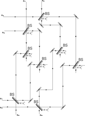
Figure 6: Circuit for the Bell-like state analyzer using ancillary qubits for assistance.

Here $\phi_{1}^{o}=\phi_{2}^{o}=\phi_{3}^{o}=\phi_{4}^{o}=\frac{\pi}{4}$ and $\phi_{1}^{e}=\phi_{2}^{e}=\phi_{3}^{e}=\phi_{4}^{e}=\theta_{2}$. It turns out that we can discriminate among $|\Gamma_{1}\rangle,|\Gamma_{2}\rangle$ and $|\Gamma_{4}\rangle$ with the success probability of

$$P_{succ}=\frac{1}{32}\left(-2\cos\left(4\theta_{2}\right)-\cos\left(2\theta_{1}\right)\left(\cos\left(4\theta_{2}\right)+3\right)+6\right)$$ (78)

Detection signatures can be summarised as:

• If output modes $\{\hat{a}^{{\dagger}}_{1}\hat{a}^{{\dagger}}_{3}\hat{a}^{{\dagger}}_{5}\hat{a}^{{\dagger}}_{7}\}$ and $\{\hat{a}^{{\dagger}}_{2}\hat{a}^{{\dagger}}_{4}\hat{a}^{{\dagger}}_{6}\hat{a}^{{\dagger}}_{8}\}$ have odd number of photons in total, states $|\Gamma_{1}\rangle$ and $|\Gamma_{2}\rangle$ are present.

  1. If $\{\hat{a}^{{\dagger}}_{1}\hat{a}^{{\dagger}}_{2}\hat{a}^{{\dagger}}_{5}\hat{a}^{{\dagger}}_{6}\}$ have even no. of photons, we can unambiguously detect $|\Gamma_{1}\rangle$.

  2. If $\{\hat{a}^{{\dagger}}_{1}\hat{a}^{{\dagger}}_{2}\hat{a}^{{\dagger}}_{5}\hat{a}^{{\dagger}}_{6}\}$ have odd no. of photons we can unambiguously detect $|\Gamma_{2}\rangle$.

• If $\{\hat{a}^{{\dagger}}_{1}\hat{a}^{{\dagger}}_{3}\hat{a}^{{\dagger}}_{5}\hat{a}^{{\dagger}}_{7}\}$ and $\{\hat{a}^{{\dagger}}_{2}\hat{a}^{{\dagger}}_{4}\hat{a}^{{\dagger}}_{6}\hat{a}^{{\dagger}}_{8}\}$ have even number of photons, states $|\Gamma_{3}\rangle$ and $|\Gamma_{4}\rangle$ are present.

  1. Furthermore if two creation operators are from the set $\{\hat{a}^{{\dagger}}_{1},\hat{a}^{{\dagger}}_{3},\hat{a}^{{\dagger}}_{5},\hat{a}^{{\dagger}}_{7}\}$ and the other two are from the set $\{\hat{a}^{{\dagger}}_{2},\hat{a}^{{\dagger}}_{4},\hat{a}^{{\dagger}}_{6},\hat{a}^{{\dagger}}_{8}\}$ only then we can uniquely detect $|\Gamma_{4}\rangle$

  2. $\{\hat{a}^{{\dagger}}_{1}\hat{a}^{{\dagger}}_{2}\hat{a}^{{\dagger}}_{3}\hat{a}^{{\dagger}}_{4}\}$ has odd photons and presence of exactly two photons in any one of the $\{\hat{a}^{{\dagger}}_{1},\hat{a}^{{\dagger}}_{3},\hat{a}^{{\dagger}}_{5},\hat{a}^{{\dagger}}_{7}\}$ is the signature for unambiguous detection for this state.

A similar thing can be done if we add another 4 extra ancillary entangled photons of the form $\big{(}\hat{a}^{{\dagger}}_{9}\hat{a}^{{\dagger}}_{11}\hat{a}^{{\dagger}}_{13}\hat{a}^{{\dagger}}_{15}\sin\left(\theta_{1}\right)+\hat{a}^{{\dagger}}_{10}\hat{a}^{{\dagger}}_{12}\hat{a}^{{\dagger}}_{14}\hat{a}^{{\dagger}}_{16}\cos\left(\theta_{1}\right)\Big{)}\ket{0}$. The variation of success probability with state parameters $\theta_{1}$ and $\theta_{2}$ is given in Fig.(7)

Figure 7: Variation of success probability of Bell-like state discrimination against state parameters – in the context of using ancilliary photon pairs in entangled states.

We observe two things:

• The success probability goes beyond $25\%$ for certain values of state parameters $\theta_{1}$ and $\theta_{2}$.

• Counterintuitively, as we increase the number of ancillary photons the success probability decreases for given values of state parameters $\theta_{1}$ and $\theta_{2}$. It still goes beyond $25\%$ in certain state parameter regimes.

If we take $\theta_{1}=\theta_{2}$ then we can unambiguously discriminate all four Bell-like states. The detection signatures remain exactly the same with extra addition being

• $\{\hat{a}^{{\dagger}}_{1}\hat{a}^{{\dagger}}_{2}\hat{a}^{{\dagger}}_{3}\hat{a}^{{\dagger}}_{4}\}$ has even photons and presence of exactly two photons in any one of the modes $\{\hat{a}^{{\dagger}}_{1},\hat{a}^{{\dagger}}_{3},\hat{a}^{{\dagger}}_{5},\hat{a}^{{\dagger}}_{7}\}$ is the signature for unambiguous detection for $|\Gamma_{3}\rangle$.

The success probability of the Bell-like state discrimination using 2 ancillary entangled photons can be calculated as

$$P_{succ}=\frac{1}{16}\sin^{2}\left(\theta_{2}\right)\left(7\cos\left(2\theta_{2}\right)+\cos\left(4\theta_{2}\right)+10\right)$$ (79)

Just like we did previously, we can add extra ancillary entangled photons of the same form for assistance and calculate the success probability. these are plotted in the Fig.(8)

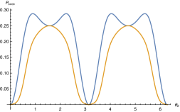
Figure 8: Variation of success probability of Bell-like state discrimination against state parameter

We again observe that for a certain value of state parameter success probability can go beyond $25\%$. Also as we increase the number of ancillary photons the success probability for a given value of the state parameter decreases. The only difference being that in latter case we can discriminate all four Bell-like states.

VII Bell-like state analysis using Non-linear elements

Besides using hyperentanglement or extra ancillary photons we can take the aid of non-linear gadgets in an aim to completely discriminate among Bell states. Four Bell-like states in a polarization basis are given as

$$|\psi_{1}\rangle=(\sin(\theta_{1})\hat{h}^{{\dagger}}_{1}\hat{h}^{{\dagger}}_{2}+\cos(\theta_{1})\hat{v}^{{\dagger}}_{1}\hat{v}^{{\dagger}}_{2})\ket{0}$$ (80)

$$|\psi_{2}\rangle=(\cos(\theta_{1})\hat{h}^{{\dagger}}_{1}\hat{h}^{{\dagger}}_{2}-\sin(\theta_{1})\hat{v}^{{\dagger}}_{1}\hat{v}^{{\dagger}}_{2})\ket{0}$$ (81)

$$|\psi_{3}\rangle=(\sin(\theta_{2})\hat{h}^{{\dagger}}_{1}\hat{v}^{{\dagger}}_{2}+\cos(\theta_{2})\hat{v}^{{\dagger}}_{1}\hat{h}^{{\dagger}}_{2})\ket{0}$$ (82)

$$|\psi_{4}\rangle=(\cos(\theta_{2})\hat{h}^{{\dagger}}_{1}\hat{v}^{{\dagger}}_{2}-\sin(\theta_{2})\hat{v}^{{\dagger}}_{1}\hat{h}^{{\dagger}}_{2})\ket{0}$$ (83)

Using Sum Frequency Generation

A non-linear process known as sum-frequency generation(SFG) is used in [22] to implement complete Bell-state analysis and then used to implement quantum teleportation with $100\%$ efficiency. A similar scheme is used here. The circuit looks like Fig.(9)

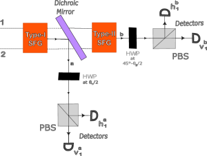
Figure 9: Circuit for the Bell-like state analyzer where non-linear processes like SFG are used to assist.

The photon pair is first passed through a non-linear crystal where it undergoes type-I SFG. Basically, pair of photons is converted into a single photon with double the frequency. Mathematically it enables the following transformation

$$\hat{h}^{{\dagger}}_{1}\hat{h}^{{\dagger}}_{2}\longrightarrow\hat{v}^{{\dagger}}_{3}$$ (84)

$$\hat{v}^{{\dagger}}_{1}\hat{v}^{{\dagger}}_{2}\longrightarrow\hat{h}^{{\dagger}}_{3}$$ (85)

This means it will only act on $|\psi_{1}\rangle$ and $|\psi_{2}\rangle$ and leave the remaining two states unchanged. The transformed states are

$$|\psi_{1}\rangle\longrightarrow(\sin(\theta_{1})\hat{v}^{{\dagger}}_{3}+\cos(\theta_{1})\hat{h}^{{\dagger}}_{3})\ket{0}$$ (86)

$$|\psi_{2}\rangle\longrightarrow(\cos(\theta_{1})\hat{v}^{{\dagger}}_{3}-\sin(\theta_{1})\hat{h}^{{\dagger}}_{3})\ket{0}$$ (87)

An important thing to note is that these states have double the frequency of the original photons. Then a dichoric mirror reflects this frequency in direction ”a” while all other frequencies are transmitted on path ”b”. On path ”a” the photon is passed through an HWP at an angle $\frac{\theta_{1}}{2}$. The final transformation looks like

$$|\psi_{1}\rangle\longrightarrow\hat{h}^{{\dagger}a}_{3}\ket{0}$$ (88)

$$|\psi_{2}\rangle\longrightarrow\hat{v}^{{\dagger}a}_{3}\ket{0}$$ (89)

Similarly in path ”b” $|\psi_{3}\rangle$ and $|\psi_{4}\rangle$ undergo type-II SFG which can be mathematically written as

$$\hat{v}^{{\dagger}}_{1}\hat{h}^{{\dagger}}_{2}\longrightarrow\hat{v}^{{\dagger}}_{3}$$ (90)

$$\hat{h}^{{\dagger}}_{1}\hat{v}^{{\dagger}}_{2}\longrightarrow\hat{h}^{{\dagger}}_{3}$$ (91)

Then the beam is allowed to fall on an HWP at an angle $45^{\circ}-\frac{\theta_{3}}{2}$. The states thus transform as

$$|\psi_{3}\rangle\longrightarrow\hat{h}^{{\dagger}b}_{3}\ket{0}$$ (92)

$$|\psi_{4}\rangle\longrightarrow\hat{v}^{{\dagger}b}_{3}\ket{0}$$ (93)

Thus we have complete Bell-like state discrimination. The signature is:

• The state is $|\psi_{1}\rangle$ if detector $h_{1}^{a}$ clicks.

• The state is $|\psi_{2}\rangle$ if detector $v_{1}^{a}$ clicks.

• The state is $|\psi_{3}\rangle$ if detector $h_{1}^{b}$ clicks.

• The state is $|\psi_{4}\rangle$ if detector $v_{1}^{b}$ clicks.

Thus we have $100\%$ success probability as compared to a scheme involving hyperentanglement where success probability is only $50\%$. Here we want to point out that the circuit used in [22] and above only differ in the orientations of the half-wave plates. Thus without the use of any extra resource in comparison to the Bell state discrimination, we can distinguish Bell-like states.

All these results can be summarised in the form of the following table:

Discrimination prtocol		Success Probability
Using Hyperentanglement
System qubits	Ancillary qubits	Bell states	Bell-like states
Polarisation DOF	Spatial DOF	$100\%$	$50\%$
Spatial DOF	Polarisation DOF	$100\%$	$50\%$
Polarisation DOF	OAM DOF	$100\%$	$50\%$
Polarisation DOF	Time DOF	$100\%$	$>25\%$ but $<50\%$
			(depends on $\theta$)
Using extra ancillary		$75\%$	$>25\%$
photon pair			(depends on $\theta_{1},\theta_{2}$)
Using SFG		$100\%$	$100\%$

VIII Conclusion and Outlook:

In this work, we explored various methods of increasing the success probability of discrimination of Bell-like states using extra resources such as hyperentanglement (entanglement in other DOF of photons), correlation in time, and ancillary entangled qubits in the backdrop of linear optics. Besides that, we have also considered the minimum amount of non-linear resources required to increase this success probability (particularly SFG).

In the case where momentum (or spatial) DOF of photons act as system qubits while polarisation DOF acts as ancillary qubits, we have seen that the success probability of Bell-like state discrimination increases from $25\%$ to $50\%$. Also, all four Bell-like states can be distinguished from each other. Comparing it to the case where we have Bell states instead we observe there also all four Bell states can be distinguished from one another. The only difference is that it is a perfect discrimination i.e. the success probability is $100\%$. Instead of the above scenario if we have polarisation DOF as system qubits and momentum DOF as system qubits we obtain the similar result. The success probability is $50\%$. Using OAM degrees of freedom as ancillary qubits while keeping polarisation DOF fixed as system qubits leads to the same observation. In all three cases, the success probability of unambiguous Bell-like state discrimination becomes $50\%$. Here, it is important to reiterate the point that the results obtained above are yet to be shown to be optimal. The optimal fidelity may be higher than $50\%$ but we guess that it is not the case. The results obtained in this paper are indeed optimal.

We have also tried to tackle the problem of Bell-like state discrimination by introducing the correlations in time DOF of two photons through the use of birefringent materials. here we obtain an interesting result. In the case of Bell state discrimination, $100\%$ success probability can be achieved through this method which automatically implies that all four Bell states can be perfectly distinguished. What we have observed is that in case of Bell-like states only three of them can be distinguished from one another. Furthermore, the success probability, although greater than $25\%$, is less than even $50\%$. Another interesting observation arises when we use ancillary qubits to distinguish between Bell-like states. In the Bell state scenario by adding two ancillary photons the optimal success probability reaches $75\%$ from $50\%$ and further increases with the number of ancillary photons. However, this is not the case with Bell-like states. firstly just by using two ancillary photons the success probability can be higher or lower than $25\%$ depending upon the state parameters $\theta_{1}$ and $\theta_{2}$. Secondly, by adding more number of ancillary photons, instead of increasing, in stark contrast to Bell states scenario, it decreases.

From the above discussion, one can conclude that discrimination of Bell-like states requires more resources as compared to discrimination of Bell states in the linear optical setting. However, we have found that when we use a non-linear element (namely SFG) for Bell-like state discrimination it can be accomplished in the same amount of resources as required for Bell state discrimination. The only difference indeed, between both setups is the orientation of the half-wave plates.

It has been shown that in a generalized three-party entanglement-swapping scenario between Alice, Bob, and Charlie where the aim is to create the state having the highest teleportation fidelity between Alice and Charlie, in some cases, it is preferable for Bob to do non-maximally entangled measurements (namely Bell-like measurements) instead of Bell measurements or any maximally entangled measurement[25]. The experimental realization of such measurements can be done with higher efficiency using the results mentioned in this paper. Also as mentioned above the optimality of the given results has still not been analyzed rigorously which can be another worthwhile direction to explore in order to understand the limitations posed by linear optical schemes in the implementation of various information-theoretical tasks.

References

• Lütkenhaus et al. [1999] N. Lütkenhaus, J. Calsamiglia, and K.-A. Suominen, Physical Review A 59, 3295 (1999).
• Kok et al. [2007] P. Kok, W. J. Munro, K. Nemoto, T. C. Ralph, J. P. Dowling, and G. J. Milburn, Rev. Mod. Phys. 79, 135 (2007).
• Azuma et al. [2015] K. Azuma, K. Tamaki, and H.-K. Lo, Nature communications 6, 6787 (2015).
• Knill et al. [2001] E. Knill, R. Laflamme, and G. J. Milburn, nature 409, 46 (2001).
• Takeda and Furusawa [2019] S. Takeda and A. Furusawa, APL Photonics 4 (2019).
• Carolan et al. [2015] J. Carolan, C. Harrold, C. Sparrow, E. Martín-López, N. J. Russell, J. W. Silverstone, P. J. Shadbolt, N. Matsuda, M. Oguma, M. Itoh, et al., Science 349, 711 (2015).
• Reck et al. [1994] M. Reck, A. Zeilinger, H. J. Bernstein, and P. Bertani, Physical review letters 73, 58 (1994).
• Tischler et al. [2018] N. Tischler, C. Rockstuhl, and K. Słowik, Phys. Rev. X 8, 021017 (2018).
• van Loock and Lütkenhaus [2004] P. van Loock and N. Lütkenhaus, Phys. Rev. A 69, 012302 (2004).
• van Loock et al. [2006] P. van Loock, K. Nemoto, W. J. Munro, P. Raynal, and N. Lütkenhaus, Phys. Rev. A 73, 062320 (2006).
• Garcia-Escartin et al. [2023] J. C. Garcia-Escartin, V. Gimeno, and J. J. Moyano-Fernández, Phys. Rev. A 108, 049901 (2023).
• Moyano-Fernández and Garcia-Escartin [2017] J. J. Moyano-Fernández and J. C. Garcia-Escartin, Optics Communications 382, 237 (2017).
• Calsamiglia and Lütkenhaus [2001] J. Calsamiglia and N. Lütkenhaus, Applied Physics B 72, 67 (2001).
• Bouwmeester et al. [1997] D. Bouwmeester, J.-W. Pan, K. Mattle, M. Eibl, H. Weinfurter, and A. Zeilinger, Nature 390, 575 (1997).
• Zhang et al. [2017] Y. Zhang, M. Agnew, T. Roger, F. S. Roux, T. Konrad, D. Faccio, J. Leach, and A. Forbes, Nature communications 8, 632 (2017).
• Schmid et al. [2009] C. Schmid, N. Kiesel, U. K. Weber, R. Ursin, A. Zeilinger, and H. Weinfurter, New Journal of Physics 11, 033008 (2009).
• Barreiro et al. [2008] J. T. Barreiro, T.-C. Wei, and P. G. Kwiat, Nature physics 4, 282 (2008).
• Williams et al. [2017a] B. P. Williams, R. J. Sadlier, and T. S. Humble, Physical review letters 118, 050501 (2017a).
• Grice [2011] W. P. Grice, Phys. Rev. A 84, 042331 (2011).
• Walborn et al. [2003] S. P. Walborn, S. Pádua, and C. H. Monken, Phys. Rev. A 68, 042313 (2003).
• Williams et al. [2017b] B. P. Williams, R. J. Sadlier, and T. S. Humble, Phys. Rev. Lett. 118, 050501 (2017b).
• Kim et al. [2001] Y.-H. Kim, S. P. Kulik, and Y. Shih, Phys. Rev. Lett. 86, 1370 (2001).
• Zaidi and van Loock [2013] H. A. Zaidi and P. van Loock, Phys. Rev. Lett. 110, 260501 (2013).
• Fields et al. [2022] D. Fields, J. A. Bergou, M. Hillery, S. Santra, and V. S. Malinovsky, Phys. Rev. A 106, 023706 (2022).
• Ghoshal et al. [2024] A. Ghoshal, J. Ghai, T. Saha, M. Alimuddin, and S. Ghosh, arXiv preprint arXiv:2401.17201  (2024).
• Kwiat and Weinfurter [1998] P. G. Kwiat and H. Weinfurter, Phys. Rev. A 58, R2623 (1998).