Skew-elliptical copula based mixed models for non-Gaussian longitudinal data with application to HIV-AIDS study

Abstract

This work has been motivated by a longitudinal data set on HIV CD4 T⁺ cell counts from Livingstone district, Zambia. The corresponding histogram plots indicate lack of symmetry in the marginal distributions and the pairwise scatter plots show non-elliptical dependence patterns. The standard linear mixed model for longitudinal data fails to capture these features. Thus it seems appropriate to consider a more general framework for modeling such data. In this article, we consider generalized linear mixed models (GLMM) for the marginals (e.g. Gamma mixed model), and temporal dependency of the repeated measurements is modeled by the copula corresponding to some skew-elliptical distributions (like skew-normal/skew-$t$). Our proposed class of copula based mixed models simultaneously takes into account asymmetry, between-subject variability and non-standard temporal dependence, and hence can be considered extensions to the standard linear mixed model based on multivariate normality. We estimate the model parameters using the IFM (inference function of margins) method, and also describe how to obtain standard errors of the parameter estimates. We investigate the finite sample performance of our procedure with extensive simulation studies involving skewed and symmetric marginal distributions and several choices of the copula. We finally apply our models to the HIV data set and report the findings.

Keywords: GLMM; longitudinal measurements; skew-elliptical distributions; copula; IFM estimation; HIV-AIDS; CD4 T⁺ cell; model selection.

1 Introduction

Biomedical studies often give rise to data where predictors and response variables are recorded at several time points. These constitute study of longitudinal data. Linear mixed models (LMMs) are the most popular class for modeling univariate longitudinal data. Normal linear mixed model was introduced in a seminal paper by Laird & Ware (1982), which extends classical linear models by introducing a subject-specific random effects to the fixed effects. This has used later extensively by statisticians in many situations (see, Verbeke & Molenberghs (1997) or Fitzmaurice et al. (2008)).

We suppose there are $m$ individuals who constitute the set of subjects. For the $i$-th ($i=1,\dots,m$) individual, repeated measurements and predictors, are recorded at $n_{i}$ time points. For each of the $n_{i}$ time points, the corresponding set of predictors are presented in a row vector of dimension $1\times p$, thus giving rise to an $n_{i}\times p$ matrix of predictors $\mathbf{X}_{i}$ and a $p\times 1$ vector of fixed effects $\mathbf{\beta}$. The $j$-th row of $\mathbf{X}_{i}$ is denoted by $\mathbf{x}_{ij}$. The set of $n_{i}$ responses is presented in an $n_{i}\times 1$ column vector denoted by $\mathbf{Y}_{i}$. Also, let us denote $\mathbf{D}_{i}$ ($n_{i}\times q$), the design matrix corresponding to the random effects, $\mathbf{b}_{i}$ of dimension $q$. Therefore, the standard linear mixed model is given by

$$\mathbf{Y}_{i}=\mathbf{X}_{i}\mathbf{\beta}+\mathbf{D}_{i}\mathbf{b}_{i}+\mathbf{\epsilon}_{i},\quad i=1,\dots,m,$$ (1.1)

where $\mathbf{\epsilon}_{i}$ ($n_{i}\times q$) is the error term. To ensure identifiability of the model, it is assumed that the collections $\{\mathbf{b}_{i}:i=1,\ldots,m\}$ and $\{\mathbf{\epsilon}_{i}:i=1,\ldots,m\}$ are independent. In the simplest setup, we assume multivariate normality of the random effects and the error terms as follows -

$$\mathbf{b}_{i}\sim N_{q}(\mathbf{0},\mathbf{\Omega}_{b}),\quad\mathbf{\epsilon}_{i}\sim N_{n_{i}}(\mathbf{0},\mathbf{\Psi}_{i}),$$ (1.2)

where $\mathbf{\Omega}_{b}$ and $\mathbf{\Psi}_{i}$ are the associated dispersion matrices that capture between-subject and within-subject variability. In many situations, it is evident from exploratory data analysis (e.g., histograms or pair-wise scatter plots) that the normality assumptions of (1.2) may not be appropriate. Generalized linear mixed models allow for different types of response distributions from the exponential family. But these models are based on conditional independence assumption of the response variables given the random effects (McCulloch (2003)).

Copulas are becoming increasingly popular tools in the literature of multivariate analysis since they allow to model and estimate joint dependence structure and the marginal distributions separately providing greater flexibility to the approach. Lambert & Vandenhende (2002) developed a Gaussian copula-based model for multivariate longitudinal data. Masarotto & Varin (2012) developed Gaussian copula based regression models for non-normal dependent observations. In recent times Killiches & Czado (2018) used D-vine copulas to model dependence between the repeated measurements for unbalanced longitudinal data. Kürüm et al. (2018) proposed a Gaussian copula based model for mixed longitudinal responses where all model parameters vary with time. In several biomedical data sets, where pair-wise scatter plots (or, normal score plots) depict asymmetric shapes, the use of standard elliptic copulas such as Gaussian or Student-$t$ are not preferable since they can not capture dependency among the time points accurately. Since any multivariate distribution can be used to construct a copula, skew-elliptical distributions (Azzalini (2013)) are appealing to introduce a flexible dependence structure into the model. Moreover, these multivariate copulas describe a general dependence structure of the model and can capture reflection, permutation asymmetry and tail dependence, if exist in the data (Chang & Joe (2020)). Das et al. (2016) previously used skew-normal copula to describe temporal dependence of univariate longitudinal data while allowing GLMMs as marginals.

Motivated from a recent HIV-AIDS CD4 count data from Livingstone district, Zambia, in this work we propose a copula based longitudinal model that accounts for temporal dependence through skew-elliptical copulas. We extend multivariate normal linear mixed model as in 1.1 in the sense that we allow GLMMs as marginals, while describing the dependence structure through some skew-elliptical distributions. Rest of the paper is organized as follows. In Section 2, we describe the data set in details which we analyzed in this paper. We describe our modeling framework in Section 3, and provide an overview of skew-elliptical distributions and their associated copulas in Section 4. In Section 5, the estimation of the model parameters using IFM method and the corresponding asymptotic normality are discussed. In Section 7, we conduct some simulation studies to monitor the parameter estimation of the proposed class of models using both skewed and symmetric marginal mixed models with different sample sizes. Section 9 concludes this article with a general discussion.

2 HIV CD4 positive T cell count data

The human immune virus (HIV) is a viral infection that slowly destroys the immune system resulting acquired immunodeficiency syndrome (AIDS). Unfortunately there is no clinically proven vaccine for this virus till today, so people rely on available antiviral drugs which slow down the viral reproduction. Most important markers for evaluating antiviral therapies are HIV-$1$ RNA copies and CD4 T⁺ cell counts. Due to the skewed nature of these two markers researchers prefer modeling these data with skew-elliptical distributions. Lin & Wang (2013) used multivariate skew-normal mixed model in ACTG $315$ study to model these markers. Bandyopadhyay et al. (2012) also considered a skew-normal based linear mixed model in a HIV viral load study.

The motivating data set analysed in this article was found in Mendeley about a recent HIV-CD4 study from Livingstone district, Zambia (2016). The data were collected during a survey of antiretroviral (ARV) combination in the treatment of HIV, as part of the work for the PhD thesis of Urban N. Haankuku at the University of South Africa and latter made publicly available. They have studied the performance of ARV combinations on HIV naive patients using several different models. According to WHO, HIV-AIDS is a major cause of death in Zambia, with about a million deaths attributed to HIV-AIDS related causes. If the disease left untreated, it can reduce the cluster of CD4 T⁺ cells and increase the HIV viral load. With non permanent cure available till today, the only option is to use antiretroviral drugs to reduce the immune suppression. The CD4 counts of $261$ HIV naive patients were measured every twelve weeks from the initial diagnosis for $48$ weeks. Three different ARV combinations were given to the patients at first baseline regimen (FBR). Covariates such as gender, age and initial weight of each patient were also reported. In Figure 1, the evolution of CD4⁺ T cell counts over time is shown. Though the mean structure is nearly linear but it reveals substantial variability between-subject responses. In Figure 2 we plot the histograms of each time point in the diagonals and pair-wise scatter plots in the off diagonals of the panel. Based on the initial diagnosis, the marginals are skewed with positive real support and the scatter plots reveals non-elliptical dependence patterns. The same thing can be observed with the normal scores, which suggests reflection and permutation asymmetry and stronger dependence than Gaussian in the joint upper and lower tails. Thus one would require more flexible dependence structure than Gaussian to model the temporal dependence. However due to the skewed nature of the CD4 counts marker with positive real support, we consider Gamma mixed model for the marginals. For comparison, we also use normal mixed model as the marginals.

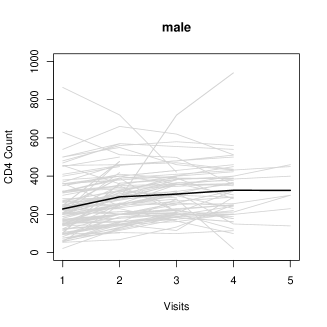
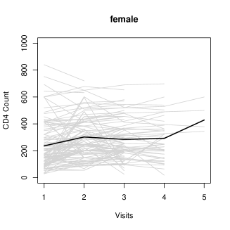
Figure 1: Individual and average profiles for male (left panel) and female (right panel) patients over time starting from initial. Black lines represent the mean profiles.

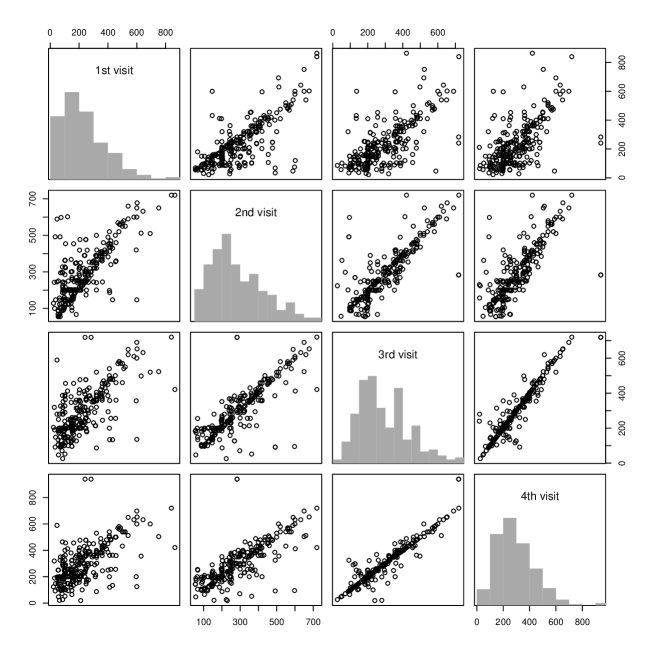
Figure 2: Pairwise scatter plots of the CD4 counts of the patients for first 4 visits.

3 A copula based longitudinal model

Let the response variables $\mathbf{Y}_{i}=(Y_{i1},\dots,Y_{in_{i}})^{\intercal},i=1,\dots,m,$ follow an $n_{i}$-variate distribution with predefined mean and dispersion matrix. Suppose observations from different individuals are independent, and to account for subject’s individual effects we consider the distribution of $\mathbf{Y}_{i}$ conditional on $\mathbf{b}_{i}$ as

$$\mathbf{Y}_{i}|\mathbf{b}_{i}\sim F_{n_{i}}(\eta(\mathbf{X}_{i}\mathbf{\beta}+\mathbf{D}_{i}\mathbf{b}_{i}),\mathbf{\Sigma}(\xi_{i},\mathbf{t}_{i}))$$ (3.1)

where $\mathbf{\xi}_{i}$ is the auto-regressive time variant parameter with respect to the time points, $\mathbf{t}_{i}=(t_{i1},\dots,t_{in_{i}})^{\intercal}$ and $\eta(.)$ is a known link function. $F_{n}(\eta,\mathbf{\Sigma})$ is an $n$-variate distribution function with mean $\eta$ and covariance $\mathbf{\Sigma}$. Furthermore, $\mathbf{X}_{i}:n_{i}\times p$ and $\mathbf{D}_{i}:n_{i}\times q$ are the known design matrices as described earlier. We assume the marginal densities of $Y_{ij}|\mathbf{b}_{i}$ are from the exponential family and functions of $\{\mathbf{x}_{ij},\mathbf{\beta},t_{ij},\mathbf{d}_{ij},\mathbf{b}_{i}\}$ via the same known link $\mathbf{\eta}(.)$. In this article we assume the random effects are independent and normally distributed, i.e. $\mathbf{b}_{i}\sim N_{q}(0,\mathbf{\Omega}_{b})$. We attempt to model such distribution using a copula based GLMM as

$$F_{n_{i}}(\mathbf{y}_{i}|\mathbf{b}_{i},\mathbf{\theta}^{*}_{i})=C_{n_{i}}(F(y_{i1}|\mathbf{b}_{i},\theta_{i1}),\dots,F(y_{in_{i}}|\mathbf{b}_{i},\theta_{in_{i}})|\mathbf{\phi}_{i})$$ (3.2)

where $\mathbf{\theta}^{*}_{i}=(\mathbf{\theta}_{i}^{\intercal},\mathbf{\phi}_{i}^{\intercal})^{\intercal}$ is the set of all vector valued parameters in the conditional model. $\mathbf{\theta}_{i}$ accounts for all the parameters present in the marginals and $\mathbf{\phi}_{i}$ accounts for the dependence parameters. Then the corresponding density function is given by

$$f_{n_{i}}(\mathbf{y}_{i}|\mathbf{b}_{i},\mathbf{\theta}^{*}_{i})=c_{n_{i}}(F(y_{i1}|\mathbf{b}_{i},\theta_{i1}),\dots,F(y_{in_{i}}|\mathbf{b}_{i},\theta_{in_{i}})|\mathbf{\phi}_{i})\prod_{j=1}^{n_{i}}f(y_{ij}|\mathbf{b}_{i},\theta_{ij}).$$ (3.3)

Copula based models are very flexible to analyze temporal dependence of longitudinal data since the responses at each point of time have a predefined marginal distribution. That is, a copula can be viewed as an association function which describes the dependence between separately specified marginals. When the marginals are fixed, many different multivariate models can be obtained from considering different copula functions. The random effects $\mathbf{b}_{i}$ are interpreted as the unobserved regression parameters for the $i$-th subject which explains variability between the subjects. The next section describes a class of multivariate copulas, which have desirable dependence properties and can be used for our models in 3.2.

4 Skew-elliptical distributions and related copulas

Multivariate skew-normal and related family of distributions proposed by Azzalini (2013) have been applied in several bio-medical studies to model non-Gaussian data. Copulas generated from skew-elliptical class of distributions can provide various flexible dependence structures. These multivariate copulas are reflection as well as permutation asymmetric and can be used to describe a general dependence structure of the model.

Definition 4.1

A random variable $\mathbf{Z}\in\mathcal{R}^{d}$ is said to have a mean zero skew-normal distribution, denoted as $\mathbf{Z}\sim SN_{d}(0,\mathbf{\Sigma,\lambda})$, if is continuous with the probability density function,

$$sn_{d}(\mathbf{z|\Sigma,\lambda})=2\phi_{d}(\mathbf{z|\Sigma})\Phi_{1}\Big{(}\mathbf{\lambda}^{\intercal}\mathbf{\Sigma}^{-1/2}\mathbf{z}\Big{)}$$ (4.1)

for $\mathbf{\lambda}\in\mathcal{R}^{d}$ and $\mathbf{\Sigma}$ be a $d\times d$ positive definite matrix. For the univariate case

$$sn_{1}(z|\sigma^{2},\lambda)=2\phi_{1}(z|\sigma^{2})\Phi_{1}\big{(}\frac{\lambda z}{\sigma}\big{)}$$ (4.2)

where $\phi_{d}(.)$ and $\Phi_{d}(.)$ are the PDF and CDF of a $d$-dimensional standard multivariate normal variable, respectively.

Skew-normal copula is obtained from the multivariate skew-normal distribution and the corresponding univariate quantiles using the probability integral transformation method. Wei et al. (2016) studied a class of copulas generated from skew-normal distribution.

Definition 4.2

A $d$-dimensional copula is said to be a skew-normal copula if

$$C_{d,SN}(\mathbf{u}|\mathbf{\Sigma,\lambda})=SN_{d}(SN_{1}^{-1}(u_{1}|1,\lambda^{*}_{1}),\dots,SN_{1}^{-1}(u_{d}|1,\lambda^{*}_{d})|\mathbf{\Sigma,\lambda})$$ (4.3)

where $SN_{1}^{-1}(u_{j}|1,\lambda^{*}_{j})$ denotes the inverse of the CDF of $Z_{j}\sim SN_{1}(1,\lambda^{*}_{j})$ distribution for $j=1,\dots,d$. The corresponding skew-normal copula density is given by

$$c_{d,SN}(\mathbf{u}|\mathbf{\Sigma,\lambda})=\frac{sn_{d}(SN_{1}^{-1}(u_{1}|1,\lambda^{*}_{1}),\dots,SN_{1}^{-1}(u_{d}|1,\lambda^{*}_{d})|\mathbf{\Sigma,\lambda})}{\prod_{j=1}^{d}sn_{1}(SN_{1}^{-1}(u_{j}|1,\lambda^{*}_{j}))}.$$ (4.4)

Here the skewness parameters ($\lambda^{*}_{j}$) of the univariate quantiles can be obtained from the multivariate parameters $\mathbf{\Sigma,\lambda}$ by

$$\lambda^{*}_{j}=\frac{\delta^{*}_{j}}{\sqrt{1-\delta^{*2}_{j}}},\;\;\text{where}\;\;\mathbf{\delta}^{*}=\mathbf{\Sigma}^{1/2}\frac{\mathbf{\lambda}}{\sqrt{1+\mathbf{\lambda}^{\intercal}\mathbf{\lambda}}}.$$ (4.5)

For more details regarding this, one can go through Azzalini & Capitanio (2003). Skew-normal copula is exchangeable or permutation symmetric if and only if $\lambda_{j}=\lambda$ for all $j=1,\dots,d$, and all off-diagonal elements of the correlation matrix $\mathbf{\Sigma}$ are equal. Note that Gaussian copula is nested to the skew-normal copula when $\lambda_{j}=0$ for all $j=1,\dots,d$.

Multivariate skew-$t$ distribution is a member of the skew-elliptical family of distribution which is defined as a scale mixture of skew-normal distribution. Gupta (2003) and Sahu et al. (2003) discussed the theoretical properties of this distribution.

Definition 4.3

Let $\mathbf{Z}\in\mathcal{R}^{d}$ be a mean zero skew-normal variable and $\mathbf{V}$ be another variable independent with $\mathbf{Z}$ such that, $\mathbf{V}\sim\mathbf{\chi}^{2}_{\mathbf{\nu}}/\mathbf{\nu}$. Then $\mathbf{T}=\mathbf{V}^{-1/2}\mathbf{Z}$ follows a mean zero skew-$t$ distribution with the probability density function,

$$st_{d}(\mathbf{t}|\mathbf{\Sigma,\lambda,\nu})=2t_{d}(\mathbf{t}|\mathbf{\Sigma,\nu})T_{1}\Bigg{(}\mathbf{\lambda}^{\intercal}\mathbf{\Sigma}^{-1/2}\mathbf{t}\sqrt{\frac{\mathbf{\nu}+d}{\mathbf{Q_{t}}+\mathbf{\nu}}}\Big{|}\mathbf{\nu}+d\Bigg{)}$$ (4.6)

where $\mathbf{Q_{t}}=\mathbf{t}^{\intercal}\mathbf{\Sigma}^{-1}\mathbf{t}$, $\mathbf{\lambda}\in\mathcal{R}^{d}$ and $\mathbf{\Sigma}$ be a $d\times d$ positive definite matrix. For the univariate case

$$st_{1}(t|\sigma^{2},\lambda,\nu)=2t_{1}(t|\sigma^{2},\nu)T_{1}\Big{(}\frac{\lambda t}{\sigma}\sqrt{\frac{\nu+1}{Q_{t}+\nu}}\Big{|}\nu+1\Big{)}$$ (4.7)

where $t_{d}(.)$ and $T_{d}(.)$ are the PDF and CDF of a $d$-dimensional standard Student-$t$ variable, respectively.

Multivariate skew-$t$ copula can be similarly obtained using the above distribution as -

Definition 4.4

A $d$-dimensional copula is said to be a skew-$t$ copula if

$$C_{d,ST}(\mathbf{u}|\mathbf{\Sigma,\lambda,\nu})=ST_{d}(ST_{1}^{-1}(u_{1}|1,\lambda^{*}_{1},\nu),\dots,ST_{1}^{-1}(u_{d}|1,\lambda^{*}_{d},\nu)|\mathbf{\Sigma,\lambda,\nu})$$ (4.8)

where $ST_{1}^{-1}(u_{j}|1,\lambda^{*}_{j},\nu)$ denotes the inverse of the CDF of $T_{j}\sim ST_{1}(1,\lambda^{*}_{j},\nu)$ distribution. The corresponding skew-t copula density is given by

$$c_{d,ST}(\mathbf{u}|\mathbf{\Sigma,\lambda,\nu})=\frac{st_{d}(ST_{1}^{-1}(u_{1}|1,\lambda^{*}_{1},\nu),\dots,ST_{1}^{-1}(u_{d}|1,\lambda^{*}_{d},\nu)|\mathbf{\Sigma,\lambda,\nu})}{\prod_{j=1}^{d}st_{1}(ST_{1}^{-1}(u_{j}|1,\lambda^{*}_{j},\nu))}.$$ (4.9)

The skew-normal copula in Definition (4.2) captures the non-exchangeable dependence between the variables of interest, with the correlation matrix $\mathbf{\Sigma}$ accounting for association between unobservable or latent variables $Z_{j}$ in (4.3) and $\mathbf{\lambda}=(\lambda_{1},\dots,\lambda_{d})^{\intercal}$ accounting for the differential skewness of the variables involved. Comparing with the skew-normal copula skew-$t$ copula in Definition (4.4) has an extra parameter known as the degrees of freedom, which accounts for possible tail dependence in the data. Yoshiba (2018) discussed the applications and maximum likelihood estimation of the skew-$t$ copula while Smith et al. (2012) discussed its Bayesian estimation. Note that for $\mathbf{\nu}\to\infty$ we have the skew-normal copula. Gaussian and Student-$t$ copula are also nested in the skew-$t$ copula. To provide some visual representations, we plot the contours of the joint densities of skew-$t$, Student-$t$, skew-normal and normal copula, using standard normal margins in Figure 3.

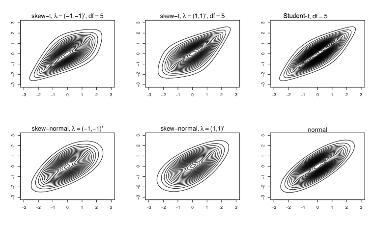
Figure 3: Contour plots of bivariate distributions using skew-$t$ copula (on the upper row) (with $\nu=5$ and $\lambda=\{(-1,-1),(1,1),(0,0)\}$) with corresponding skew-normal copula (on the lower row); the common correlation parameter $\rho=0.77$ and common marginals are standard normal.

5 Parameter estimation

In Section 3 we described a class of copula based longitudinal models. However for such models which involves complex non-exchangeable multivariate copulas as described in Section 4, parameter estimation is not often evident, especially in moderate to high-dimensional situations. Furthermore, direct maximum likelihood estimation is not always feasible, because of the time consuming computation of the quantiles of the skew-elliptical copulas. Hence we employ a fully parametric estimation method known as Inference Function for Margins (IFM) to estimate the parameters for the class of models in (3.2). When the likelihood function of the data analytic model is computationally difficult to work with, Joe & Xu (1996) introduced this two stage maximum likelihood estimation method in which all parameters present in the model are estimated in two steps. Joe (2005) discussed asymptotic efficiency of this method where the univariate parameters are estimated from separate univariate likelihoods at the first stage, and then the multivariate parameters are estimated from the multivariate likelihood with the univariate parameters given the values from the first stage.

For the class of models in (3.2) we implement the IFM method to estimate the model parameters and their standard errors using the corresponding asymptotic covariance matrix. Since the response variables $\mathbf{Y}_{i}$ are conditionally independent, the joint density of the $i$-th response is

$$f_{n_{i}}(\mathbf{y}_{i},\mathbf{b}_{i}|\mathbf{\theta}^{*}_{i})=f_{n_{i}}(\mathbf{y}_{i}|\mathbf{b}_{i},\mathbf{\theta}^{*}_{i})g(\mathbf{b}_{i}).$$ (5.1)

In the presence of unobserved random effects, in the first stage we consider each marginal responses $y_{ij}|\mathbf{b}_{i}$ are conditionally independent. Therefore, we construct the inference functions as

$$l^{*}_{i}(\mathbf{\theta}_{i}|\mathbf{y}_{i}) =\log\int\prod_{j=1}^{n_{i}}f(y_{ij}|\mathbf{b}_{i},\theta_{ij})g(\mathbf{b}_{i})d\mathbf{b}_{i},$$

$$l^{*}_{i}(\mathbf{\theta}^{*}_{i}|\mathbf{y}_{i}) =\log\int c_{n_{i}}(F(y_{i1}|\mathbf{b}_{i},\theta_{i1}),\dots,F(y_{in_{i}}|\mathbf{b}_{i},\theta_{in_{i}})|\mathbf{\phi}_{i})\prod_{j=1}^{n_{i}}f(y_{ij}|\mathbf{b}_{i},\theta_{ij})g(\mathbf{b}_{i})d\mathbf{b}_{i}.$$ (5.2)

Now to obtain the IFM estimates based on $m$ independent observations we assume, $\mathbf{\theta}^{*}_{i}=(\mathbf{\theta}_{i}^{\intercal},\mathbf{\phi}_{i}^{\intercal})^{\intercal}$ are all functions of $\mathbf{\theta}^{*}=(\mathbf{\theta}^{\intercal},\mathbf{\phi}^{\intercal})^{\intercal}$ for $i=1,\dots,m$. For notational simplicity, we assume that the parameters of the random effects distribution is included in $\mathbf{\theta}$ and $\mathbf{\phi}$ includes the dependence parameters as in (3.3). The IFM method estimates the model parameters by

$$\hat{\mathbf{\theta}} =\arg\underset{\mathbf{\theta}}{\max}\sum_{i=1}^{m}l^{*}_{i}(\mathbf{\theta}_{i}|\mathbf{y}_{i}),$$

$$\hat{\mathbf{\phi}} =\arg\underset{\mathbf{\phi}}{\max}\sum_{i=1}^{m}l^{*}_{i}(\hat{\mathbf{\theta}_{i}},\mathbf{\phi}_{i}|\mathbf{y}_{i})$$ (5.3)

and the estimating equations for $\mathbf{\theta}$ and $\mathbf{\phi}$ based on IFM are

$$\Psi_{1m}(\mathbf{\theta})=\sum_{i=1}^{m}\Psi_{i1m}(\mathbf{\theta}) =\sum_{i=1}^{m}\frac{\partial}{\partial\mathbf{\theta}}l^{*}_{i}(\mathbf{\theta}_{i}|\mathbf{y}_{i})=\mathbf{0},$$

$$\Psi_{2m}(\mathbf{\phi})=\sum_{i=1}^{m}\Psi_{i2m}(\mathbf{\phi}) =\sum_{i=1}^{m}\frac{\partial}{\partial\mathbf{\phi}}l^{*}_{i}(\hat{\mathbf{\theta}_{i}},\mathbf{\phi}_{i}|\mathbf{y}_{i})=\mathbf{0}$$ (5.4)

provided the derivatives exist. The IFM estimates are obtained either by numerically maximizing (5) or by solving the system of non-linear equations as in (5).

5.1 Asymptotic normality

Here we show under some regularity conditions, the IFM estimators for the class of models in (3.2) are consistent and asymptotically normal. We also present the theoretical analysis for independent and non-identically distributed (i.n.i.d) observations including random effects. Let us denote the true value of the parameters $\mathbf{\theta^{*}}=(\mathbf{\theta}^{\intercal},\mathbf{\phi}^{\intercal})^{\intercal}$ by $\mathbf{\theta}^{*}_{0}=(\mathbf{\theta}_{0}^{\intercal},\mathbf{\phi}_{0}^{\intercal})^{\intercal}$ and let $\Psi^{*}_{im}=(\Psi_{i1m}^{\intercal},\Psi_{i2m}^{\intercal})^{\intercal}$ be the stack of the vector valued inference function for the $i$-th response. To establish the consistency and asymptotic normality, we need the set of assumptions in Appendix A, which make $\Psi^{*}_{m}=\sum_{i=1}^{m}\Psi^{*}_{im}$ a regular inference function vector and consequently we have the following theorem.

Theorem 5.1

Consider the model (3.2) and let $\hat{\mathbf{\theta}}^{*}=(\hat{\mathbf{\theta}}^{\intercal},\hat{\mathbf{\phi}}^{\intercal})^{\intercal}$ denote the IFME of $\mathbf{\theta^{*}}$ corresponding to IFM (5). Under the assumptions in Appendix A, $\hat{\mathbf{\theta}}^{*}$ is a consistent estimator of $\mathbf{\theta^{*}}$. Furthermore, as $m\rightarrow\infty$, we have asymptotic normality as

$$\sqrt{m}(\hat{\mathbf{\theta}}^{*}-\mathbf{\theta}^{*}_{0})\;\;\overset{d}{\rightarrow}N(\mathbf{0},J_{\Psi}(\mathbf{\theta}^{*}_{0})^{-1}),\;\;\text{where}\;\;J_{\Psi}(\mathbf{\theta}^{*}_{0})=D_{\Psi}(\mathbf{\theta}^{*}_{0})^{\intercal}M_{\Psi}(\mathbf{\theta}^{*}_{0})^{-1}D_{\Psi}(\mathbf{\theta}^{*}_{0}),$$

$$M_{\Psi}(\mathbf{\theta}^{*}_{0})=\lim_{m\rightarrow\infty}\frac{1}{m}\sum_{i=1}^{m}E[\Psi_{im}(\mathbf{\theta}^{*}_{0})\Psi_{im}(\mathbf{\theta}^{*}_{0})^{\intercal}]\;\;\text{and}\;\;D_{\Psi}(\mathbf{\theta}^{*}_{0})=\lim_{m\rightarrow\infty}\frac{1}{m}\sum_{i=1}^{m}E\Big{[}\frac{\partial}{\partial\mathbf{\theta}^{*}}\Psi_{im}(\mathbf{\theta^{*}})\Big{|}_{\mathbf{\theta}^{*}_{0}}\Big{]}.$$

Based on the general discussions in Xu (1996), we also provide a simplified proof of the above theorem in Appendix A. Verification of the regularity assumptions for the class of considered models is difficult and beyond the scope of this paper. Note that, here $M_{\Psi}(\mathbf{\theta}^{*}_{0})$ and $D_{\Psi}(\mathbf{\theta}^{*}_{0})$ both depends on the distribution of the random effects $\mathbf{b}_{i}$. The asymptotic covariance matrix in (5.1) is known as Godambe information matrix in the literature. The observed version of this matrix can be numerically obtained by

$$M_{\Psi}(\hat{\mathbf{\theta}}^{*}) =\frac{1}{m}\sum_{i=1}^{m}\Psi_{im}(\mathbf{\theta^{*}})\Big{|}_{\hat{\mathbf{\theta}}^{*}}\Psi_{im}(\mathbf{\theta^{*}})^{\intercal}\Big{|}_{\hat{\mathbf{\theta}}^{*}},$$

$$D_{\Psi}(\hat{\mathbf{\theta}}^{*}) =\frac{1}{m}\sum_{i=1}^{m}\left(\begin{array}[]{cc}\frac{\partial}{\partial\mathbf{\theta}}\Psi_{i1m}(\mathbf{\theta})\Big{|}_{\hat{\mathbf{\theta}}}&\mathbf{0}\\ \mathbf{0}&\frac{\partial}{\partial\mathbf{\phi}}\Psi_{i2m}(\mathbf{\phi})\Big{|}_{\hat{\mathbf{\phi}}}\end{array}\right),$$ (5.7)

which leads to a straightforward calculation of the standard errors for the parameter estimates based on IFM (5), using the square-roots of the diagonals of $J_{\Psi}(\hat{\mathbf{\theta}}^{*})^{-1}$. We employed numerical derivative methods to obtain the matrices in (5.1).

5.2 Numerical implementation

As we described in Section 3, we consider generalized linear mixed models for the marginals of the class of models in (3.2). Gamma distribution with $\log$ link is a good candidate, when the response distributions are seen to be asymmetric with positive real support. The Gamma distributed response variable $Y_{ij}$ with shape parameter $\kappa$ and mean $\eta_{ij}$ has the density

$$f(y_{ij}|\eta_{ij},\kappa)=\Gamma^{-1}(\kappa)\Big{(}\frac{\eta_{ij}}{\kappa}\Big{)}^{-1}y_{ij}^{-k}\exp\Big{(}-\frac{y_{ij}\kappa}{\eta_{ij}}\Big{)}.$$ (5.8)

For comparison, we also consider a symmetric marginal distribution such as normal with mean $\eta_{ij}$ and variance $\sigma^{2}$, having the density

$$f(y_{ij}|\eta_{ij},\sigma^{2})=\frac{1}{\sqrt{2\pi}\sigma}\exp\Big{(}-\frac{1}{2}\Big{(}\frac{y_{ij}-\eta_{ij}}{\sigma}\Big{)}^{2}\Big{)}.$$ (5.9)

To evaluate the integrations in (5), we use standard Gauss-Hermite quadrature rule with $15$ quadrature points. The matrices in (5.1) are obtained similarly, to compute the standard errors of the parameter estimates.

The serial correlation of the repeated measurements is characterized in the correlation matrix of the skew-elliptical copulas. $\mathbf{\Sigma}$ present in (3.1) is taken as a function of time and dispersion parameter $\mathbf{\xi}$ (time-varying serial dependence). Corresponding to the estimating model in (3.2), we assume homogeneous variance ($\sigma^{2}$ or $1/\kappa)$ within units and consider AR-1 structure for the correlation matrix $\mathbf{\Sigma}$ in the skew-elliptical copulas. This correlation structure is used when the observations are equally spaced. Here we implement exponential autocorrelation function defined as

$$Corr(Y_{ij},Y_{ik})=\exp\left(-\mathbf{\xi}|t_{ij}-t_{ik}|\right),\quad\mathbf{\xi}\geq 0,$$ (5.10)

to construct the correlation matrix $\mathbf{\Sigma}(\xi,\mathbf{t}_{i})$ of the class of skew-elliptical copulas. This structural assumption is made based on the sample correlation matrix of our data. Similarly one can adopt an exchangeable correlation matrix depending upon the data. IFM method estimates the model parameters in two stages but it is not efficient as direct maximum likelihood estimation. As shown by Kim et al. (2007), a slight bias from the first stage of IFM estimation can introduce significant disturbance in the copula parameter estimation in the second stage. In our case we have seen that leaving the skewness parameter of the skew-normal and skew-$t$ copula unrestricted, results in either heavily biased estimation of that parameter or not finding the optimal solution. Since for longitudinal data, same sample is observed across time, we assume same value for the skewness parameter $\mathbf{\lambda}$ for each dimension (equi-skewness). These structures not only reduce the number of estimable parameters from the model but also ensure the positive definiteness of the correlation matrices during the estimation process. For the numerical optimizations we use optim function in R with L-BFGS-B method. In the following section we discuss the comparison between different fitted models to the data.

6 Model comparison

A problem intrinsic to analysis of longitudinal data is model choice, or determining the number of components that is most appropriate for a specific data set. For the class of models in (3.2) one need to choose appropriate marginal distributions along with the multivariate copula. For this purpose the log-likelihood based measures such as AIC (Akaike information criterion) and BIC (Bayesian information criterion), which penalize large number of parameters, are frequently applied. AIC and BIC are defined by

$$AIC=-2l(\hat{\mathbf{\theta}}^{*})+2\dim(\hat{\mathbf{\theta}}^{*}),\;\;BIC=-2l(\hat{\mathbf{\theta}}^{*})+\log(m)\dim(\hat{\mathbf{\theta}}^{*})$$ (6.1)

where $\hat{\mathbf{\theta}}^{*}$ is the maximum likelihood estimates of the model parameters and $m$ is the sample size. Whereas the penalty of the AIC only depends on the number of parameters in the model, that of BIC also depends on the sample size. However when we employ two stage maximum likelihood estimation for the class of models these information criteria are modified accordingly in the literature (Jordanger & Tjøstheim (2014)). Here we assume that the true data generating model is included in the set of candidate models. Ko & Hjort (2019) showed that if the marginals and the copula family are correctly specified, then the two-stage AIC coincides with the original. Similar justifications are discussed in Killiches & Czado (2018) (Remark 1). Based on that, in our approach we use these as close approximations of the true AIC and BIC by plugging in the two-stage estimates in the actual likelihood functions evaluated by numerical quadrature integration.

7 Simulation design and analysis

Simulation studies are conducted to illustrate the performance of IFM estimation for the proposed class of multivariate models in (3.2). The goal of this study is to monitor the parameter inference using IFM estimation with different combinations of copulas and marginal distributions. We have used two different sample sizes, $m=\{200,500\}$ and fixed the dimension of each response vectors to $n_{i}=4$. Since the true parameters are known, to generate the response variable $\mathbf{Y}_{i}|\mathbf{b}_{i}$, we first sample from the multivariate copulas discussed in section 4 with similar values of the dependence parameters, $(\mathbf{\xi,\lambda,\nu})^{\intercal}$. Then we use probability integral transformation to generate per-unit multivariate response $\mathbf{Y}_{i}|\mathbf{b}_{i}$. We assume the distribution of the random effects to be normal for all the cases. Mainly due to increase in computation time, we restrict with random intercept structure in the linear predictor of the models. Note that, in (5), we use a straight forward GLMM estimation at the first stage, which makes the considered models comparable. While keeping the marginal distributions fixed, we compare the parameter estimates with $4$ choices of the multivariate copulas. To obtain the initial estimates of the marginal parameters we use nlme package in R, and then the initial values of the dependence parameters are obtained from fitting the rescaled empirical CDF (uniform data) to the copulas. Furthermore, for the skew-$t$ and Student-$t$ copulas we used fixed integer valued degrees of freedom parameter $\mathbf{\nu}$.

The following class of models investigates the parameter estimation under both binary and categorical variables present as covariates, in order to mimic the real data discussed in the following section. We denote the general structure of the models with both fixed and random effects with time-varying dependence as

$$\mathbf{Y}_{i}|\mathbf{b}_{i} \sim F_{n_{i}}(\eta(\mathbf{X}_{i}\mathbf{\beta}+\mathbf{D}_{i}\mathbf{b}_{i}),\mathbf{\Sigma}(\xi,\mathbf{t}_{i}))$$

$$\text{with}\;\;x_{ij}\mathbf{\beta}+d_{ij}\mathbf{b}_{i} =\beta_{0}+x_{1i}\beta_{1}+x_{2i}\beta_{2}+t_{ij}\beta_{3}+b_{i},$$ (7.1)

where $F_{n_{i}}$ is a multivariate distribution with link function $\eta$ as described in (3.1). We set here $\beta_{0}=1.5$, $\beta_{1}=0.5$, $\beta_{2}=0.5$ and $\beta_{3}=1.0$ for the fixed effect parameters. Here $x_{1i}=1*I(i\leq m/2)+2*I(i>m/2)$, and $x_{2i}=0$ or $1$ assigned randomly ($m$ is the sample size). The random effects are set as $b_{i}\sim N(0,1)$ and the time points $t_{ij}=j-2.5$ for $j=1,\dots,n_{i}$. In one scenario we use Gamma distribution with log-link and shape parameter $\kappa=3$ for the marginals. In the other scenario we use normal distribution with standard deviation $\sigma=1$. For the correlation matrix in all the multivariate copulas we set the time difference per observation within each response vector to unity. Hence the off-diagonal entries of the matrix $\mathbf{\Sigma(\xi)}$ are

$$\mathbf{\rho}(t_{ij},t_{ik})=\exp(-\mathbf{\xi}|j-k|),\quad 1\leq j<k\leq n_{i}.$$ (7.2)

Here we consider skew-$t$ and skew-normal copula along with their symmetric counterparts for the dependence structure of the models. We set $\mathbf{\xi}=0.25$ for all the copulas. For the skew-elliptical ones we set $\bar{\mathbf{\lambda}}=1$ under equi-skewness, and fixed values for the degrees of freedom parameter as $\mathbf{\nu}=\{3,8,15\}$. For each simulation we generate $N=500$ Monte Carlo samples and then estimate the parameters and their associated standard errors.

	Parameters	$\beta_{0}$	$\beta_{1}$	$\beta_{2}$	$\beta_{3}$	$V[b]$	$\kappa$	$\mathbf{\xi}$	$\bar{\mathbf{\lambda}}$
	True Value	1.5	0.5	0.5	1.0	1.0	3.0	0.25	1.0
Copula	Skew-t,$\mathbf{\nu}=3$
m = 200	Mean	1.4917	0.5054	0.4967	1.0001	0.9890	3.3965	0.3171	0.6465
	Bias	-0.0083	0.0054	-0.0033	0.0001	-0.0110	0.3965	0.0671	-0.3535
	SD	0.2598	0.1542	0.1525	0.0208	0.1820	1.1862	0.1192	0.3294
	SE	0.2800	0.1850	0.1971	0.0317	0.2002	1.9486	0.0423	0.2934
	RMSE	0.2599	0.1543	0.1525	0.0208	0.1823	1.2507	0.1368	0.4832
m = 500	Mean	1.4921	0.5068	0.4953	0.9999	0.9929	3.2168	0.2848	0.7376
	Bias	-0.0079	0.0068	-0.0047	-0.0001	-0.0071	0.2168	0.0348	-0.2624
	SD	0.1712	0.1003	0.1025	0.0117	0.1211	0.7187	0.0738	0.2283
	SE	0.1680	0.0934	0.1107	0.0158	0.1064	0.6521	0.0249	0.2426
	RMSE	0.1714	0.1005	0.1026	0.0117	0.1213	0.7507	0.0816	0.3478
Copula	Skew-t,$\mathbf{\nu}=8$
m = 200	Mean	1.5115	0.4933	0.5020	1.0024	0.9678	3.3293	0.3307	0.6405
	Bias	0.0115	-0.0067	0.0020	0.0024	-0.0322	0.3293	0.0807	-0.3595
	SD	0.2687	0.1610	0.1574	0.0188	0.1849	1.2072	0.1410	0.3908
	SE	0.2829	0.1336	0.1754	0.0310	0.1458	1.5335	0.0416	0.3185
	RMSE	0.2689	0.1611	0.1575	0.0189	0.1878	1.2513	0.1625	0.5310
m = 500	Mean	1.4945	0.5025	0.4978	1.0008	1.0003	3.2085	0.3087	0.6910
	Bias	-0.0055	0.0025	-0.0022	0.0008	0.0003	0.2085	0.0587	-0.3090
	SD	0.1700	0.1014	0.1003	0.0124	0.1282	0.7294	0.0886	0.2289
	SE	0.1621	0.0773	0.1069	0.0178	0.0804	0.8080	0.0251	0.2005
	RMSE	0.1700	0.1014	0.1004	0.0125	0.1282	0.7587	0.1063	0.3845
Copula	Skew-t,$\mathbf{\nu}=15$
m = 200	Mean	1.5158	0.4904	0.4935	0.9989	0.9712	3.3751	0.3432	0.6272
	Bias	0.0158	-0.0096	-0.0065	-0.0011	-0.0288	0.3751	0.0932	-0.3728
	SD	0.2655	0.1546	0.1517	0.0198	0.1884	1.2154	0.1563	0.4076
	SE	0.2718	0.1504	0.1751	0.0310	0.1509	1.7044	0.0426	0.3271
	RMSE	0.2659	0.1549	0.1519	0.0198	0.1906	1.2719	0.1810	0.5524
m = 500	Mean	1.4984	0.5003	0.5015	0.9997	0.9994	3.1865	0.3086	0.6926
	Bias	-0.0016	0.0003	0.0015	-0.0003	-0.0006	0.1865	0.0586	-0.3074
	SD	0.1711	0.0981	0.0982	0.0128	0.1272	0.6829	0.0873	0.2690
	SE	0.1573	0.0742	0.1000	0.0158	0.0785	0.6281	0.0248	0.2171
	RMSE	0.1711	0.0981	0.0982	0.0128	0.1272	0.7080	0.1052	0.4085
Copula	Skew-normal
m = 200	Mean	1.4854	0.5080	0.5098	1.0024	0.9750	3.3101	0.3554	0.5956
	Bias	-0.0146	0.0080	0.0098	0.0024	-0.0250	0.3101	0.1054	-0.4044
	SD	0.2629	0.1546	0.1563	0.0210	0.1843	1.1463	0.1621	0.3980
	SE	0.2920	0.1406	0.2132	0.0387	0.1661	1.5973	0.0472	0.3602
	RMSE	0.2633	0.1548	0.1565	0.0212	0.1860	1.1876	0.1933	0.5674
m = 500	Mean	1.4891	0.5039	0.5017	1.0001	0.9884	3.1932	0.3211	0.6771
	Bias	-0.0109	0.0039	0.0017	0.0001	-0.0116	0.1932	0.0711	-0.3229
	SD	0.1765	0.1009	0.0948	0.0121	0.1249	0.7273	0.1005	0.2788
	SE	0.1576	0.0735	0.0990	0.0157	0.0791	0.7316	0.0258	0.2033
	RMSE	0.1768	0.1009	0.0949	0.0121	0.1255	0.7525	0.1231	0.4266

Table 1: Parameter estimation using IFM method when the marginals are distributed as Gamma. Performance for $500$ replications with skew-$t$ and skew-normal copula.

	Parameters	$\beta_{0}$	$\beta_{1}$	$\beta_{2}$	$\beta_{3}$	$V[b]$	$\kappa$	$\mathbf{\xi}$	$\bar{\mathbf{\lambda}}$
	True Value	1.5	0.5	0.5	1.0	1.0	3.0	0.25	-
Copula	Student-t,$\mathbf{\nu}=3$
m = 200	Mean	1.4864	0.5049	0.5004	1.0002	0.9782	3.5281	0.2811	-
	Bias	-0.0136	0.0049	0.0004	0.0002	-0.0218	0.5281	0.0311	-
	SD	0.2704	0.1567	0.1644	0.0169	0.1831	1.4162	0.1049	-
	SE	0.2963	0.2271	0.2142	0.0441	0.2264	2.1010	0.0243	-
	RMSE	0.2708	0.1568	0.1644	0.0169	0.1844	1.5114	0.1094	-
m = 500	Mean	1.4922	0.4982	0.5029	0.9999	1.0026	3.3119	0.2702	-
	Bias	-0.0078	-0.0018	0.0029	-0.0001	0.0026	0.3119	0.0202	-
	SD	0.1725	0.0997	0.1014	0.0098	0.1354	0.8041	0.0646	-
	SE	0.1945	0.0791	0.1323	0.0144	0.0895	1.3090	0.0153	-
	RMSE	0.1727	0.0997	0.1015	0.0098	0.1355	0.8625	0.0677	-
Copula	Student-t,$\mathbf{\nu}=8$
m = 200	Mean	1.5173	0.4930	0.4892	0.9996	0.9842	3.4324	0.2822	-
	Bias	0.0173	-0.0070	-0.0108	-0.0004	-0.0158	0.4324	0.0322	-
	SD	0.2819	0.1692	0.1582	0.0160	0.1904	1.2955	0.1074	-
	SE	0.3126	0.1634	0.2097	0.0320	0.1812	2.1569	0.0223	-
	RMSE	0.2824	0.1694	0.1585	0.0160	0.1911	1.3658	0.1122	-
m = 500	Mean	1.5118	0.4953	0.4958	0.9998	0.9939	3.1866	0.2636	-
	Bias	0.0118	-0.0047	-0.0042	-0.0002	-0.0061	0.1866	0.0137	-
	SD	0.1730	0.0979	0.1017	0.0105	0.1411	0.7289	0.0670	-
	SE	0.1649	0.0773	0.1035	0.0138	0.1118	0.6927	0.0135	-
	RMSE	0.1734	0.0980	0.1017	0.0106	0.1413	0.7524	0.0683	-
Copula	Student-t,$\mathbf{\nu}=15$
m = 200	Mean	1.4785	0.5077	0.5058	1.0004	0.9943	3.5381	0.2953	-
	Bias	-0.0215	0.0077	0.0058	0.0004	-0.0057	0.5381	0.0453	-
	SD	0.2665	0.1613	0.1647	0.0171	0.1843	1.2716	0.1122	-
	SE	0.2860	0.1512	0.1967	0.0343	0.1752	2.2277	0.0223	-
	RMSE	0.2673	0.1615	0.1648	0.0171	0.1844	1.3808	0.1210	-
m = 500	Mean	1.4941	0.5032	0.4931	0.9999	0.9930	3.2570	0.2716	-
	Bias	-0.0059	0.0032	-0.0069	-0.0001	-0.0070	0.2570	0.0216	-
	SD	0.1788	0.1029	0.1065	0.0102	0.1330	0.7906	0.0715	-
	SE	0.1683	0.0818	0.1083	0.0142	0.0837	0.7635	0.0132	-
	RMSE	0.1789	0.1029	0.1067	0.0102	0.1332	0.8313	0.0748	-
Copula	Gaussian
m = 200	Mean	1.4976	0.4988	0.4987	0.9999	0.9722	3.4854	0.2925	-
	Bias	-0.0024	-0.0012	-0.0013	-0.0001	-0.0278	0.4854	0.0425	-
	SD	0.2643	0.1597	0.1660	0.0163	0.1953	1.3667	0.1264	-
	SE	0.2879	0.1429	0.2174	0.0337	0.1844	1.7209	0.0209	-
	RMSE	0.2643	0.1597	0.1660	0.0163	0.1973	1.4504	0.1333	-
m = 500	Mean	1.4985	0.5006	0.4991	1.0000	0.4937	3.2284	0.2725	-
	Bias	-0.0015	0.0006	-0.0009	0.0000	-0.0063	0.2284	0.0225	-
	SD	0.1780	0.1039	0.1025	0.0096	0.1320	0.7880	0.0778	-
	SE	0.1616	0.0766	0.1030	0.0142	0.0812	0.6222	0.0125	-
	RMSE	0.1781	0.1040	0.1025	0.0096	0.1321	0.8204	0.0809	-

Table 2: Parameter estimation using IFM method when the marginals are distributed as Gamma. Performance for $500$ replications with Student-$t$ and Gaussian copula.

	Parameters	$\beta_{0}$	$\beta_{1}$	$\beta_{2}$	$\beta_{3}$	$V[b]$	$\sigma$	$\mathbf{\xi}$	$\bar{\mathbf{\lambda}}$
	True Value	1.5	0.5	0.5	1.0	1.0	1.0	0.25	1.0
Copula	Skew-t,$\mathbf{\nu}=3$
m = 200	Mean	1.4713	0.5115	0.5102	1.0002	1.0388	0.9768	0.2753	0.6528
	Bias	-0.0287	0.0115	0.0102	0.0002	0.0388	-0.0232	0.0253	-0.3472
	SD	0.3010	0.1882	0.1765	0.0307	0.1674	0.1411	0.0965	0.2841
	SE	0.2722	0.1300	0.1744	0.0308	0.2206	0.1874	0.0694	0.2932
	RMSE	0.3113	0.1886	0.1768	0.0307	0.1736	0.1430	0.1000	0.4486
m = 500	Mean	1.4886	0.5039	0.5071	0.9990	1.0370	0.9771	0.2744	0.6586
	Bias	-0.0114	0.0039	0.0071	-0.0010	0.0374	-0.0229	0.0244	-0.3414
	SD	0.1929	0.1174	0.1139	0.0210	0.1055	0.0756	0.0656	0.1700
	SE	0.1694	0.0818	0.1106	0.0196	0.0947	0.0677	0.0447	0.1784
	RMSE	0.1933	0.1174	0.1141	0.0210	0.1120	0.0720	0.0700	0.3901
Copula	Skew-t,$\mathbf{\nu}=8$
m = 200	Mean	1.4944	0.5033	0.5101	0.9990	1.0370	0.9771	0.2771	0.6282
	Bias	-0.0056	0.0033	0.0101	-0.0010	0.0370	-0.0229	0.0271	-0.3718
	SD	0.2751	0.1728	0.1711	0.0311	0.1583	0.1320	0.0920	0.3209
	SE	0.2697	0.1278	0.1714	0.0307	0.2076	0.1965	0.0720	0.3146
	RMSE	0.2752	0.1729	0.1714	0.0311	0.1626	0.1340	0.0959	0.4911
m = 500	Mean	1.5046	0.4976	0.5020	1.0002	1.0349	0.9784	0.2764	0.6915
	Bias	0.0046	-0.0024	0.0020	0.0002	0.0349	-0.0216	0.0264	-0.3085
	SD	0.1859	0.1120	0.1107	0.0189	0.1059	0.0989	0.0520	0.1556
	SE	0.1689	0.0812	0.1094	0.0195	0.0943	0.0762	0.0382	0.1449
	RMSE	0.1860	0.1120	0.1107	0.0189	0.1115	0.1012	0.0583	0.3455
Copula	Skew-t,$\mathbf{\nu}=15$
m = 200	Mean	1.5035	0.4960	0.5011	1.0018	1.0370	0.9773	0.2767	0.6409
	Bias	0.0035	-0.0040	0.0011	0.0018	0.0370	-0.0227	0.0267	-0.3591
	SD	0.2921	0.1747	0.1734	0.0292	0.1594	0.1292	0.0801	0.2943
	SE	0.2663	0.1274	0.1721	0.0311	0.2256	0.1952	0.0670	0.2516
	RMSE	0.2922	0.1747	0.1734	0.0293	0.1636	0.1312	0.0844	0.4643
m = 500	Mean	1.4981	0.5037	0.5009	1.0018	1.0367	0.9775	0.2767	0.6887
	Bias	-0.0019	0.0037	0.0009	0.0010	0.0367	-0.0225	0.0267	-0.3113
	SD	0.1835	0.1102	0.1057	0.0200	0.1042	0.0887	0.0513	0.1672
	SE	0.1695	0.0815	0.1097	0.0195	0.0927	0.0723	0.0363	0.1457
	RMSE	0.1845	0.1105	0.1057	0.0200	0.1105	0.0915	0.0578	0.3534
Copula	Skew-normal
m = 200	Mean	1.4982	0.4987	0.5097	0.9986	1.0386	0.9775	0.2768	0.6307
	Bias	-0.0018	-0.0013	0.0097	-0.0014	0.0386	-0.0225	0.0268	-0.3693
	SD	0.2889	0.1750	0.1821	0.0319	0.1587	0.1275	0.0791	0.3435
	SE	0.2704	0.1292	0.1723	0.0309	0.2309	0.2162	0.0650	0.2810
	RMSE	0.2889	0.1750	0.1824	0.0319	0.1633	0.1295	0.0835	0.5044
m = 500	Mean	1.4984	0.4990	0.5021	0.9997	1.0381	0.9977	0.2764	0.6963
	Bias	-0.0016	-0.0010	0.0021	-0.0003	0.0381	-0.0223	0.0264	-0.3037
	SD	0.1911	0.1156	0.1109	0.0196	0.0981	0.0859	0.0451	0.1563
	SE	0.1708	0.0839	0.1099	0.0195	0.0818	0.0745	0.0332	0.1509
	RMSE	0.1911	0.1156	0.1109	0.0196	0.1052	0.0887	0.0523	0.3416

Table 3: Parameter estimation using IFM method when the marginals are distributed as normal. Performance for $500$ replications with skew-$t$ and skew-normal copula.

	Parameters	$\beta_{0}$	$\beta_{1}$	$\beta_{2}$	$\beta_{3}$	$V[b]$	$\sigma$	$\mathbf{\xi}$	$\bar{\mathbf{\lambda}}$
	True Value	1.5	0.5	0.5	1.0	1.0	1.0	0.25	-
Copula	Student-t,$\mathbf{\nu}=3$
m = 200	Mean	1.4715	0.5208	0.4996	1.0014	1.0560	0.9627	0.2855	-
	Bias	-0.0285	0.0208	-0.0004	0.0014	0.0560	-0.0373	0.0355	-
	SD	0.3126	0.1852	0.1884	0.0258	0.1862	0.1124	0.1471	-
	SE	0.3352	0.2044	0.2088	0.0621	0.2129	0.0998	0.0887	-
	RMSE	0.3139	0.1864	0.1884	0.0258	0.1944	0.1184	0.1513	-
m = 500	Mean	1.5017	0.4986	0.4995	0.9989	1.0584	0.9635	0.2837	-
	Bias	0.0017	-0.0014	-0.0005	-0.0011	0.0584	-0.0365	0.0337	-
	SD	0.2007	0.1200	0.1176	0.0158	0.1242	0.0804	0.1020	-
	SE	0.1982	0.0968	0.1307	0.0229	0.1476	0.0507	0.0487	-
	RMSE	0.2007	0.1200	0.1176	0.0158	0.1372	0.0883	0.1074	-
Copula	Student-t,$\mathbf{\nu}=8$
m = 200	Mean	1.4872	0.5041	0.5054	0.9991	1.0557	0.9630	0.2909	-
	Bias	-0.0128	0.0041	0.0054	-0.0009	0.0557	-0.0370	0.0409	-
	SD	0.3053	0.1881	0.1871	0.0256	0.1716	0.1125	0.1427	-
	SE	0.3361	0.2035	0.2067	0.0608	0.2111	0.1333	0.0888	-
	RMSE	0.3056	0.1881	0.1872	0.0256	0.1804	0.1184	0.1484	-
m = 500	Mean	1.5067	0.4963	0.5041	0.9994	1.0495	0.9633	0.2861	-
	Bias	0.0115	-0.0027	0.0041	-0.0006	0.0495	-0.0361	0.0361	-
	SD	0.1918	0.1211	0.1211	0.0154	0.1214	0.0816	0.0978	-
	SE	0.1985	0.0951	0.1273	0.0241	0.1126	0.0549	0.0427	-
	RMSE	0.1923	0.1212	0.1212	0.0156	0.1311	0.0892	0.1042	-
Copula	Student-t,$\mathbf{\nu}=15$
m = 200	Mean	1.5067	0.5052	0.4917	0.9998	1.0026	0.9814	0.2643	-
	Bias	0.0067	0.0052	-0.0083	-0.0002	0.0026	-0.0186	0.0143	-
	SD	0.3109	0.1900	0.1893	0.0238	0.1568	0.1200	0.1414	-
	SE	0.3356	0.1810	0.1921	0.0256	0.1869	0.1312	0.0799	-
	RMSE	0.3109	0.1901	0.1895	0.0238	0.1570	0.1214	0.1429	-
m = 500	Mean	1.4939	0.5044	0.5021	0.9998	1.0022	0.9908	0.2567	-
	Bias	-0.0061	0.0044	0.0021	-0.0002	0.0022	-0.0092	0.0067	-
	SD	0.1937	0.1203	0.1146	0.0153	0.1076	0.0784	0.0955	-
	SE	0.1748	0.0843	0.1134	0.0154	0.0889	0.0561	0.0433	-
	RMSE	0.1938	0.1203	0.1147	0.0153	0.1078	0.0786	0.0957	-
Copula	Gaussian
m = 200	Mean	1.4982	0.5082	0.4927	0.9993	1.0066	0.9836	0.2633	-
	Bias	-0.0018	0.0082	-0.0073	-0.0007	0.0066	-0.0164	0.0133	-
	SD	0.3053	0.1885	0.1860	0.0233	0.1512	0.1102	0.1377	-
	SE	0.3153	0.1315	0.1775	0.0293	0.1732	0.1242	0.0751	-
	RMSE	0.3053	0.1885	0.1861	0.0233	0.1514	0.1114	0.1383	-
m = 500	Mean	1.4988	0.5070	0.5038	1.0010	1.0060	0.9928	0.2557	-
	Bias	-0.0012	0.0070	0.0038	0.0010	0.0060	-0.0072	0.0057	-
	SD	0.2047	0.1255	0.1210	0.0160	0.1037	0.0777	0.0951	-
	SE	0.1754	0.0842	0.1135	0.0153	0.0843	0.0543	0.0447	-
	RMSE	0.2051	0.1256	0.1210	0.0160	0.1039	0.0780	0.0953	-

Table 4: Parameter estimation using IFM method when the marginals are distributed as normal. Performance for $500$ replications with Student-$t$ and Gaussian copula.

Table 1 and 2 show parameter estimations of the class of models in (7) using skew-elliptical and elliptical copulas and gamma marginals with Gaussian random effects. We present the mean, the biases [$\frac{1}{N}\sum_{i=1}^{N}(\hat{\theta}^{*}_{j}-\theta^{*})$], roots of mean square errors [$\sqrt{\frac{1}{N}\sum_{i=1}^{N}(\hat{\theta}^{*}_{j}-\theta^{*})^{2}}$], empirical standard errors (denoted as SD) and the standard errors obtained from the asymptotic covariance matrices (denoted as SE), where $\hat{\theta}^{*}_{j}$ is the parameter estimates for the $j$-th sample. In Table 3 and 4, we provide additional simulation results using normal marginals as well. The results show that parameter estimations tend to have higher accuracies based on larger sample size $m$ with smaller Bias, SE and RMSE. However, there is systematic bias in the estimation of the skewness parameter $\bar{\mathbf{\lambda}}$ for all the models, and the shape parameter $\kappa$ for the Gamma based models. We notice that using IFM method does not change the precision of estimation of the marginal parameters very much. Overall, the estimation of parameters are accurate and SE and SD are relatively close to each other, which shows this estimating approach is viable for drawing inference from real data set.

8 Data analysis

Due to the skewed nature of the CD4 count marker with positive real support, we intend to model the marginals using Gamma mixed model and the temporal dependence using skewed multivariate copulas to assess the disease progression. Our model investigates the change in CD4 counts across time within patients. We have seen that the $\log$ or square root transformation doesn’t take away the skewness completely. We make a scale transformation of the CD4⁺ T cell counts by $100$ for easier estimation and interpretation of the coefficients. Only a few entries were seen in the $5$-th visit column, hence we omit it from our analysis. Some entries were missing in the $4$-th visit column and we imputed those entries using carry forward method (Suresh et al. (2021)). We take the predictors as age, gender, first baseline regimen and initial weight of each patient. Gender indicators $0$ is used for female and $1$ for a male patient respectively. First base regimen (FBR) of ARV combination is indicated as $1,2$ and $5$. Therefore, referring to the models in (3.1) we consider -

$$x_{ij}\beta+d_{ij}\mathbf{b}_{i}=\beta_{0}+\mathrm{gender}_{i}\beta_{1}+\mathrm{age}_{i}\beta_{2}+\mathrm{fbr}_{i}\beta_{3}+\mathrm{weight}_{i}\beta_{4}+t_{ij}\beta_{5}+b_{i},$$ (8.1)

and $Y_{ij}$ is the CD4 count at $j$-th time point for the $i$-th patient (normalized by $100$). The time variable is rescaled as $t_{ij}=(\mathrm{week}-18)/12$. We have considered random intercept structure in the models. Based on the sample correlation matrix of this data set, AR(1) structure for the correlation matrices for the multivariate copulas seems to be appropriate. After the rescaling of the time points, the entries of the correlation matrix $\mathbf{\Sigma_{i}}$, are equivalent to $\mathbf{\rho}(t_{ij},t_{ik})=\exp(-\mathbf{\xi}|j-k|),\;\;1\leq k<j\leq n_{i}$. Considering two marginal mixed models with four multivariate copulas, we estimate the parameters using the method described in Section 5. Since we use fixed integer valued $\mathbf{\nu}$ in the skew-$t$ and Student-$t$ copula, we select the value with in the set $\{3,\dots,30\}$ based on the maximum value of the log-likelihood.

	Gamma marginals		Normal marginals
Parameters	Est.	SE	Est.	SE
$\beta_{0}$	0.2533	0.1558	1.3204	0.4558
$\beta_{1}$	0.0959	0.0539	0.1264	0.1454
$\beta_{2}$	0.0025	0.0019	0.0011	0.0049
$\beta_{3}$	0.0114	0.0154	0.0201	0.0408
$\beta_{4}$	0.0113	0.0015	0.0273	0.0042
$\beta_{5}$	0.0907	0.0103	0.2022	0.0269
$V[b]$	0.0700	0.0258	1.2140	0.3390
$\kappa$	5.0979	1.9562	-	-
$\sigma$	-	-	0.8890	0.1394

Table 5: Marginal parameter estimation of HIV CD4⁺ T cell count data with model (8.1) using Gamma and normal mixed model.

Gamma marginals
Copula	degrees of freedom ($\mathbf{\nu}$)	3	4	5	6
Skew-$t$	Log-likelihood	-1250.84	-1261.45	-1272.17	-1281.84
Student-$t$	Log-likelihood	-1288.30	-1304.63	-1338.77	-1347.63
Normal marginals
Copula	degrees of freedom ($\mathbf{\nu}$)	3	4	5	6
Skew-$t$	Log-likelihood	-1256.88	-1271.31	-1285.62	-1296.17
Student-$t$	Log-likelihood	-1257.02	-1271.50	-1285.89	-1297.65

Table 6: Estimation of the degrees of freedom parameter for the skew-$t$ and Student-$t$ copula based on the maximum log-likelihood.

Model	Copula	Parameters	Est.	SE	Log-likelihood	AIC	BIC
Gamma	Skew-$t$,$\mathbf{\nu}=3$	$\mathbf{\xi}$	0.1781	0.0190	-1250.84	2521.67	2557.32
		$\bar{\mathbf{\lambda}}$	1.2765	0.5373
	Skew-normal	$\mathbf{\xi}$	0.1904	0.0329	-1422.96	2863.92	2895.99
		$\bar{\mathbf{\lambda}}$	1.8547	0.4033
	Student-$t$,$\mathbf{\nu}=3$	$\mathbf{\xi}$	0.2052	0.0256	-1288.30	2594.60	2626.68
	Gaussian	$\mathbf{\xi}$	0.4525	0.0810	-1468.57	2953.14	2981.65
Normal	Skew-$t$,$\mathbf{\nu}=3$	$\mathbf{\xi}$	0.2611	0.0285	-1256.88	2535.77	2594.98
		$\bar{\mathbf{\lambda}}$	-0.0156	0.0650
	Skew-normal	$\mathbf{\xi}$	0.3084	0.0481	-1429.61	2879.21	2914.86
		$\bar{\mathbf{\lambda}}$	-0.5016	0.0850
	Student-$t$,$\mathbf{\nu}=3$	$\mathbf{\xi}$	0.2612	0.0285	-1257.02	2534.04	2569.68
	Gaussian	$\mathbf{\xi}$	0.5358	0.1113	-1480.53	2979.05	3011.13

Table 7: Dependence parameter estimation of HIV CD4⁺ T cell count data with model (8.1). Maximum log-likelihood value, AIC and BIC for the skew-$t$, skew-normal, Student-$t$ and Gaussian copula respectively.

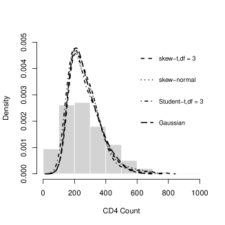
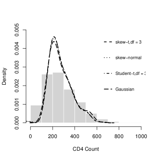
Figure 4: Fitting of HIV CD4⁺ T cell count data with model (8.1) using Gamma marginals (left panel) and normal marginals (right panel). The histograms show the frequency distribution of observed CD4 counts with different dotted lines representing the fitted models.

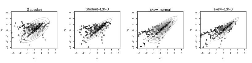
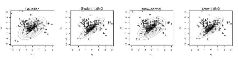
Figure 5: Fitting of the copula data (transformed to standard normal margins) using Gamma (upper panel) and normal mixed model (lower panel) of the first two time points, including the contour lines of the fitted skew and elliptical copulas, respectively.

Since with the IFM estimation method, the marginal parameter estimates are eventually same for all the multivariate copula based models, therefore in Table 5, we summarise the marginal parameter estimates and the corresponding standard errors for the mixed model (8.1) with Gamma and normal marginals when the copula is Gaussian. In Table 6 we show the estimation of the fixed degrees of freedom parameter for the skew-$t$ and Student-$t$ copula based on maximum log-likelihood. Finally in Table 7, we present the dependence parameter estimates, the corresponding standard errors with the log-likelihood (of the full model), AIC and BIC, for the skew-$t$, skew-normal, Student-$t$ and Gaussian copula, respectively. We estimate the random effects from the posterior modes, for each subject under different multivariate models. This enables us to plot the models graphically when the unobserved random effects are estimated. Figure 4 shows the histograms of the CD4 counts of $261$ HIV patients and the dotted lines are the fitted models with two marginals and four multivariate copulas respectively. Similarly, using the estimated random effects, we transform the data into normal scores using the cumulative distribution functions of the marginals ($F(.)$). In Figure 5 we provide the contour plots of the fitted skew and elliptical copulas to the data of the first two time points using two different marginal distributions.

From this analysis, we can see that the estimates of $\beta_{2}$ are close to zero under both marginal models. That implies age has minor impact on the disease progression. On other hand based on the estimate of $\beta_{1}$, gender has a much significant effect on the HIV progression, which is previously indicated in the profile plots in 1. The effect of time as a covariate is significant as shown by the estimate of $\beta_{5}$. Based on the selection criteria, we see that skew-$t$ copula based Gamma mixed model provide with the best fit to the data, among the eight candidate models. Smaller value of the degrees of freedom parameter implies stronger tail dependence across time in the data. The estimates of the skewness parameter indicates reflection and permutation asymmetry when the marginals are assumed to be Gamma. But with the normal marginals these estimates are lower with negative values. This may be caused due to the fact that when marginals are modeled with some symmetric distributions, it undermines the asymmetry in both the marginals and the dependence structure. Therefore, with the copula based modeling, one should prioritize for proper choice of the marginals with computational tractability. Overall, the considered class of copula based mixed models performs reasonably well since we are able to estimate $13$ coefficients for $261$ observations quite accurately.

9 Conclusion and summary

In this paper, we studied an extension of classical linear mixed model based on multivariate normality. Motivated from a real world HIV data set, we developed skew-elliptical copula based generalized linear mixed models to analyze the data. The standard linear mixed model is treated as a special case in our construction. When the data set violates normality, our proposed class of models provide with better fit while capturing reflection, permutation asymmetry and tail dependence, if present in the data. We apply our methods to model the disease progression using CD4 T⁺ cell counts of the HIV data set. Our considered class of models have a general dependence structure as of the skew-elliptical distributions which makes easier interpretation of the dependence parameters. In our analysis, we saw that use of skew-$t$ copula based Gamma mixed model provides the best fit out of eight candidate models.

We obtain the standard errors of the parameter estimates using the corresponding asymptotic covariance matrix (Godambe information matrix) of IFM estimation. Our simulation study illustrates the performance of IFM estimation of model parameters with various choices of multivariate copulas and marginal distributions. However, even with IFM estimation, skew-$t$ and skew-normal copula based models takes significantly more computation time than Student-$t$ and Gaussian copula based models. Gauss-Hermite quadrature rule is applied to carry out the numerical integrations, but the computational burden increases exponentially with the dimension of the random effects. In future studies we want to investigate some other estimation methods for the proposed class of models, which can provide one step estimation of the model parameters. Bayesian methods might be useful in this context, for which one can assess the effect of copula in the estimation of the regression coefficients. We are also interested in incorporating missing data mechanism for the class of models to make them more general and versatile.

Appendix A Appendix

Assumptions for Theorem 5.1:

1. The support of $\mathbf{Z}=(\mathbf{Y}^{\intercal},\mathbf{b}^{\intercal})^{\intercal}$, $\mathcal{Z}$ does not depend on any $\mathbf{\theta^{*}}\in\mathbf{\Theta^{*}}$.

2. The partial derivatives $\partial\Psi^{*}_{m}/\partial\mathbf{\theta^{*}}$ exist for almost every $\mathbf{z}\in\mathcal{Z}$.

3. (a) For all $\mathbf{\theta^{*}}\in\mathbf{\Theta^{*}}$,

   $$\frac{1}{m}\sum_{i=1}^{m}\Psi_{i1m}(\mathbf{\theta}) \overset{p}{\rightarrow}\lim_{m\rightarrow\infty}\frac{1}{m}\sum_{i=1}^{m}E[\Psi_{i1m}(\mathbf{\theta})]=\mathbf{0},$$

   $$\frac{1}{m}\sum_{i=1}^{m}\Psi_{i2m}(\mathbf{\phi}) \overset{p}{\rightarrow}\lim_{m\rightarrow\infty}\frac{1}{m}\sum_{i=1}^{m}E[\Psi_{i2m}(\mathbf{\phi})]=\mathbf{0}.$$

   (b) For all $\mathbf{\theta^{*}}\in\mathbf{\Theta^{*}}$,

   $$E[\Psi_{im}(\mathbf{\theta^{*}})\Psi_{im}(\mathbf{\theta^{*}})^{\intercal}]\;\;\text{and}\;\;\lim_{m\rightarrow\infty}\frac{1}{m}\sum_{i=1}^{m}E[\Psi_{im}(\mathbf{\theta^{*}})\Psi_{im}(\mathbf{\theta^{*}})^{\intercal}]\;\;\text{exist},$$

   and $$\frac{1}{m}\sum_{i=1}^{m}\Psi_{im}(\mathbf{\theta^{*}})\Psi_{im}(\mathbf{\theta^{*}})^{\intercal}\overset{p}{\rightarrow}\lim_{m\rightarrow\infty}\frac{1}{m}\sum_{i=1}^{m}E[\Psi_{im}(\mathbf{\theta^{*}})\Psi_{im}(\mathbf{\theta^{*}})^{\intercal}]=M_{\Psi}(\mathbf{\theta^{*}})$$

   where $M_{\Psi}(\mathbf{\theta^{*}})$ is a positive definite matrix.

   $$E\Big{[}\frac{\partial}{\partial\mathbf{\theta^{*}}}\Psi_{im}(\mathbf{\theta^{*}})\Big{]}\;\;\text{exists},\;\text{and}\;\;\frac{1}{m}\sum_{i=1}^{m}\frac{\partial}{\partial\mathbf{\theta^{*}}}\Psi_{im}(\mathbf{\theta^{*}})\overset{p}{\rightarrow}\lim_{m\rightarrow\infty}\frac{1}{m}\sum_{i=1}^{m}E\Big{[}\frac{\partial}{\partial\mathbf{\theta^{*}}}\Psi_{im}(\mathbf{\theta^{*}})\Big{]}=D_{\Psi}(\mathbf{\theta^{*}})$$

   where $D_{\Psi}(\mathbf{\theta^{*}})$ is a non-singular matrix.

4. The order of integration and difference can be interchanged as follows

   $$\frac{\partial}{\partial\mathbf{\theta^{*}}}\int_{\mathcal{Z}}f^{*}(z,\mathbf{\theta^{*}})dz=\int_{\mathcal{Z}}\frac{\partial}{\partial\mathbf{\theta^{*}}}f^{*}(z,\mathbf{\theta^{*}})dz.$$

5. For all $\epsilon>0$ and for any fixed vector $\mathbf{u},(||\mathbf{u}||\neq 0)$, the following condition is satisfied.

   $$\lim_{m\rightarrow\infty}\frac{1}{m}\sum_{i=1}^{m}E\Big{[}(\mathbf{u}^{\intercal}\Psi_{im}(\mathbf{\theta}^{*}_{0}))^{2}I\Big{\{}|\mathbf{u}^{\intercal}\Psi_{im}(\mathbf{\theta}^{*}_{0})|\geq\epsilon\sqrt{m}\Big{\}}\Big{]}=0.$$

Proof of Thorem 5.1: Using Taylor’s (Lagrange) expansion to the first order, we have

$$\Psi_{1m}(\hat{\mathbf{\theta}}) =\Psi_{1m}(\mathbf{\theta}_{0})+(\hat{\mathbf{\theta}}-\mathbf{\theta}_{0})\frac{\partial}{\partial\mathbf{\theta}}\Psi_{1m}(\mathbf{\theta})\Big{|}_{\mathbf{\theta}_{1}},$$

$$\Psi_{2m}(\hat{\mathbf{\phi}}) =\Psi_{2m}(\mathbf{\phi}_{0})+(\hat{\mathbf{\phi}}-\mathbf{\phi}_{0})\frac{\partial}{\partial\mathbf{\phi}}\Psi_{2m}(\mathbf{\phi})\Big{|}_{\mathbf{\phi}_{1}}$$ (A.1)

where $\mathbf{\theta}_{1}$ is some vector value between $\mathbf{\theta}_{0}$ and $\hat{\mathbf{\theta}}$, and $\mathbf{\phi}_{1}$ is some vector value between $\mathbf{\phi}_{0}$ and $\hat{\mathbf{\phi}}$, respectively. Note that $\Psi_{2m}(\hat{\mathbf{\phi}})$ also depends on the value $\hat{\mathbf{\theta}}$. Assumption $3$(a) implies

$$E\Big{[}\frac{\partial}{\partial\mathbf{\theta}}\log\int\prod_{j=1}^{n_{i}}f(y_{ij}|\mathbf{b_{i}},\theta_{ij})g(\mathbf{b_{i}})d\mathbf{b_{i}}\Big{]}$$

exists and naught for all $i=1,\dots,m$. Thus we have

$$\frac{1}{m}\Psi_{1m}(\mathbf{\theta}_{0})\overset{p}{\rightarrow}\mathbf{0},\;\;\frac{1}{m}\Psi_{2m}(\mathbf{\phi}_{0})\overset{p}{\rightarrow}\mathbf{0}.$$

Also from assumption $3$(b), the expectations of

$$\frac{1}{m}\frac{\partial}{\partial\mathbf{\theta}}\Psi_{1m}(\mathbf{\theta})\;\;\text{and}\;\;\frac{1}{m}\frac{\partial}{\partial\mathbf{\phi}}\Psi_{2m}(\mathbf{\phi})$$

converges to non-zero real vectors almost surely. Since all terms on the right hand side converges to zero, when $\hat{\mathbf{\theta}}$ and $\hat{\mathbf{\phi}}$ are the solutions of 5. Hence we must have

$$\hat{\mathbf{\theta}}\overset{p}{\rightarrow}\mathbf{\theta}_{0}\;\;\text{and}\;\;\hat{\mathbf{\phi}}\overset{p}{\rightarrow}\mathbf{\phi}_{0}.$$

To derive the asymptotic normality let

$$H_{m}(\mathbf{\theta^{*}})=\left(\begin{array}[]{cc}\frac{\partial}{\partial\mathbf{\theta}}\Psi_{1m}(\mathbf{\theta})&\mathbf{0}\\ \\ \mathbf{0}&\frac{\partial}{\partial\mathbf{\phi}}\Psi_{2m}(\mathbf{\phi})\end{array}\right)\;\;\text{and}\;\;H_{m}^{1}=\left(\begin{array}[]{cc}\frac{\partial}{\partial\mathbf{\theta}}\Psi_{1m}(\mathbf{\theta})\Big{|}_{\mathbf{\theta}_{1}}&\mathbf{0}\\ \\ \mathbf{0}&\frac{\partial}{\partial\mathbf{\phi}}\Psi_{2m}(\mathbf{\phi})\Big{|}_{\mathbf{\phi}}\end{array}\right)$$

We rewrite the expression in A as

$$\sqrt{m}(\hat{\mathbf{\theta}}^{*}-\mathbf{\theta}^{*}_{0})=\Big{[}\frac{1}{m}H_{m}^{1}\Big{]}^{-1}\frac{1}{\sqrt{m}}[-\Psi_{m}(\mathbf{\theta}^{*}_{0})].$$ (A.2)

Since $\hat{\mathbf{\theta}}^{*}$ is a consistent estimator of $\mathbf{\theta}^{*}_{0}$, from the convergence in probability we have

$$\frac{1}{m}[H_{m}(\hat{\mathbf{\theta}}^{*})-H_{m}(\mathbf{\theta}^{*}_{0})]\overset{p}{\rightarrow}\mathbf{0}.$$

Now from assumption $3$(b) we have,

$$\frac{1}{m}H_{m}(\mathbf{\theta}^{*}_{0})=\left(\begin{array}[]{cc}\frac{1}{m}\sum_{i=1}^{m}\frac{\partial}{\partial\mathbf{\theta}}\Psi_{i1m}(\mathbf{\theta})\Big{|}_{\mathbf{\theta}_{0}}&\mathbf{0}\\ \\ \mathbf{0}&\frac{1}{m}\sum_{i=1}^{m}\frac{\partial}{\partial\mathbf{\phi}}\Psi_{i2m}(\mathbf{\phi})\Big{|}_{\mathbf{\phi}}\end{array}\right)\;\;\overset{p}{\rightarrow}D_{\Psi}(\mathbf{\theta}^{*}_{0}).$$

Thereafter using assumption $3$(b) and $4$ we get,

$$\frac{1}{m^{2}}Cov[H_{m}(\mathbf{\theta}^{*}_{0})] =\frac{1}{m^{2}}\sum_{i=1}^{m}Cov\Big{[}\frac{\partial}{\partial\mathbf{\theta^{*}}}\Psi_{im}(\mathbf{\theta^{*}})\Big{|}_{\mathbf{\theta}^{*}_{0}}$$

$$=\frac{1}{m}\Big{[}\frac{1}{m}\sum_{i=1}^{m}E\Big{[}\frac{\partial}{\partial\mathbf{\theta^{*}}}\Psi_{im}(\mathbf{\theta^{*}})\Big{|}_{\mathbf{\theta}^{*}_{0}}\frac{\partial}{\partial\mathbf{\theta^{*}}^{\intercal}}\Psi_{im}(\mathbf{\theta^{*}})^{\intercal}\Big{|}_{\mathbf{\theta}^{*}_{0}}\Big{]}$$

$$=\frac{1}{m}\Big{[}\frac{1}{m}\sum_{i=1}^{m}\frac{\partial^{2}}{\partial\mathbf{\theta^{*}}\partial\mathbf{\theta^{*}}^{\intercal}}E\Big{[}\Psi_{im}(\mathbf{\theta^{*}})\Big{|}_{\mathbf{\theta}^{*}_{0}}\Psi_{im}(\mathbf{\theta^{*}})^{\intercal}\Big{|}_{\mathbf{\theta}^{*}_{0}}\Big{]}\;\;\rightarrow\mathbf{0}\;\;\text{as}\;\;m\rightarrow\infty.$$

Now $\mathbf{\theta}^{*}_{1}$ lies in between $\hat{\mathbf{\theta}}^{*}$ and $\mathbf{\theta}^{*}_{0}$, thus by weak law of large number

$$\frac{1}{m}H_{m}^{1}-D_{\Psi}(\mathbf{\theta}^{*}_{0})\;\;\overset{p}{\rightarrow}\mathbf{0}.$$

The final term of the expression A.2, $\Psi_{m}(\mathbf{\theta}^{*}_{0})$ involves sum of independent terms, which have expectation $\mathbf{0}$ and covariance matrix $Cov[\Psi_{im}(\mathbf{\theta}^{*}_{0})]=E[\Psi_{im}(\mathbf{\theta}^{*}_{0})\Psi_{im}(\mathbf{\theta}^{*}_{0})^{\intercal}]$ for $i=1,\dots,m$. Hence from assumption $5$, with direct application of Lindeberg-Feller central limit theorem, for any fixed vector $\mathbf{u}$ we have,

$$\mathbf{u}^{\intercal}\Big{(}\frac{\Psi_{m}(\mathbf{\theta}^{*}_{0})}{\sqrt{m}}\Big{)}\;\;\overset{d}{\rightarrow}N(0,\mathbf{u}^{\intercal}M_{\Psi}(\mathbf{\theta}^{*}_{0})\mathbf{u})$$

Combining everything and using Slutsky’s theorem we finally have,

$$\sqrt{m}(\hat{\mathbf{\theta}}^{*}-\mathbf{\theta}^{*}_{0})\;\;\overset{d}{\rightarrow}N(\mathbf{0},J_{\Psi}(\mathbf{\theta}^{*}_{0})^{-1}),\;\;\text{where}\;\;J_{\Psi}(\mathbf{\theta}^{*}_{0})=D_{\Psi}(\mathbf{\theta}^{*}_{0})^{\intercal}M_{\Psi}(\mathbf{\theta}^{*}_{0})^{-1}D_{\Psi}(\mathbf{\theta}^{*}_{0}),$$

and that completes the proof.

References

- (1)
- Azzalini (2013) Azzalini, A. (2013), The skew-normal and related families (IMS Monographs), Vol. 3, Cambridge University Press.
- Azzalini & Capitanio (2003) Azzalini, A. & Capitanio, A. (2003), ‘Distributions generated by perturbation of symmetry with emphasis on a multivariate skew t-distribution’, Journal of the Royal Statistical Society: Series B (Statistical Methodology) 65(2), 367–389.
- Bandyopadhyay et al. (2012) Bandyopadhyay, D., Lachos, V. H., Castro, L. M. & Dey, D. K. (2012), ‘Skew-normal/independent linear mixed models for censored responses with applications to hiv viral loads’, Biometrical Journal 54(3), 405–425.
- Chang & Joe (2020) Chang, B. & Joe, H. (2020), ‘Copula diagnostics for asymmetries and conditional dependence’, Journal of Applied Statistics 47(9), 1587–1615.
- Das et al. (2016) Das, K., Elmasri, M. & Sen, A. (2016), ‘A skew-normal copula-driven glmm’, Statistica Neerlandica 70(4), 396–413.
- Fitzmaurice et al. (2008) Fitzmaurice, G., Davidian, M., Verbeke, G. & Molenberghs, G. (2008), Longitudinal Data Analysis (Handbook), Vol. 1, Chapman and Hall/CRC press.
- Gupta (2003) Gupta, A. (2003), ‘Multivariate skew t-distribution’, Statistics: A Journal of Theoretical and Applied Statistics 37(4), 359–363.
- Joe (2005) Joe, H. (2005), ‘Asymptotic efficiency of the two-stage estimation method for copula-based models’, Journal of Multivariate Analysis 94(2), 401–419.
- Joe & Xu (1996) Joe, H. & Xu, J. J. (1996), ‘The estimation method of inference functions for margins for multivariate models’, Technical Report, University of British Columbia 166, 22.
- Jordanger & Tjøstheim (2014) Jordanger, L. A. & Tjøstheim, D. (2014), ‘Model selection of copulas: Aic versus a cross validation copula information criterion’, Statistics & Probability Letters 92, 249–255.
- Killiches & Czado (2018) Killiches, M. & Czado, C. (2018), ‘A d-vine copula-based model for repeated measurements extending linear mixed models with homogeneous correlation structure’, Biometrics 74(3), 997–1005.
- Kim et al. (2007) Kim, G., Silvapulle, M. J. & Silvapulle, P. (2007), ‘Comparison of semiparametric and parametric methods for estimating copulas’, Computational Statistics & Data Analysis 51(6), 2836–2850.
- Ko & Hjort (2019) Ko, V. & Hjort, N. L. (2019), ‘Copula information criterion for model selection with two-stage maximum likelihood estimation’, Econometrics and Statistics 12, 167–180.
- Kürüm et al. (2018) Kürüm, E., Hughes, J., Li, R. & Shiffman, S. (2018), ‘Time-varying copula models for longitudinal data’, Statistics and its Interface 11(2), 203–221.
- Laird & Ware (1982) Laird, N. M. & Ware, J. H. (1982), ‘Random-effects models for longitudinal data’, Biometrics 38, 963–974.
- Lambert & Vandenhende (2002) Lambert, P. & Vandenhende, F. (2002), ‘A copula-based model for multivariate non-normal longitudinal data: analysis of a dose titration safety study on a new antidepressant’, Statistics in Medicine 21(21), 3197–3217.
- Lin & Wang (2013) Lin, T.-I. & Wang, W.-L. (2013), ‘Multivariate skew-normal at linear mixed models for multi-outcome longitudinal data’, Statistical Modelling 13(3), 199–221.
- Masarotto & Varin (2012) Masarotto, G. & Varin, C. (2012), ‘Gaussian copula marginal regression’, Electronic Journal of Statistics 6, 1517–1549.
- McCulloch (2003) McCulloch, C. E. (2003), ‘Generalized linear mixed models’, NSF-CBMS Regional Conference Series in Probability and Statistics 7, 84.
- Sahu et al. (2003) Sahu, S. K., Dey, D. K. & Branco, M. D. (2003), ‘A new class of multivariate skew distributions with applications to bayesian regression models’, Canadian Journal of Statistics 31(2), 129–150.
- Smith et al. (2012) Smith, M. S., Gan, Q. & Kohn, R. J. (2012), ‘Modelling dependence using skew t copulas: Bayesian inference and applications’, Journal of Applied Econometrics 27(3), 500–522.
- Suresh et al. (2021) Suresh, K., Taylor, J. M. & Tsodikov, A. (2021), ‘A gaussian copula approach for dynamic prediction of survival with a longitudinal biomarker’, Biostatistics 22(3), 504–521.
- Verbeke & Molenberghs (1997) Verbeke, G. & Molenberghs, G. (1997), Linear Mixed Models for Longitudinal Data, Vol. 1, Springer, New York.
- Wei et al. (2016) Wei, Z., Kim, S. & Kim, D. (2016), ‘Multivariate skew normal copula for non-exchangeable dependence’, Procedia Computer Science 91, 141–150.
- Xu (1996) Xu, J. J. (1996), Statistical modelling and inference for multivariate and longitudinal discrete response data, PhD thesis, University of British Columbia.
- Yoshiba (2018) Yoshiba, T. (2018), ‘Maximum likelihood estimation of skew-t copulas with its applications to stock returns’, Journal of Statistical Computation and Simulation 88(13), 2489–2506.