Recasting Regional Lighting for Shadow Removal

Abstract

Removing shadows requires an understanding of both lighting conditions and object textures in a scene. Existing methods typically learn pixel-level color mappings between shadow and non-shadow images, in which the joint modeling of lighting and object textures is implicit and inadequate. We observe that in a shadow region, the degradation degree of object textures depends on the local illumination, while simply enhancing the local illumination cannot fully recover the attenuated textures. Based on this observation, we propose to condition the restoration of attenuated textures on the corrected local lighting in the shadow region. Specifically, We first design a shadow-aware decomposition network to estimate the illumination and reflectance layers of shadow regions explicitly. We then propose a novel bilateral correction network to recast the lighting of shadow regions in the illumination layer via a novel local lighting correction module, and to restore the textures conditioned on the corrected illumination layer via a novel illumination-guided texture restoration module. We further annotate pixel-wise shadow masks for the SRD dataset, which originally contains only image pairs. Experiments on three benchmarks show that our method outperforms existing SOTA shadow removal methods.

Introduction

Shadows manifest on surfaces where light is partially or entirely blocked, resulting in image areas with reduced intensity, darker colors, and diminished textures. These shadows can create recognition ambiguities in existing visual models, such as text recognition (Brown and Tsoi 2006), remote traffic monitoring (Zhang et al. 2020b), and object localization (Mei et al. 2021; Liu et al. 2023a). Consequently, the study of shadow removal becomes crucial.

There are a number of shadow removal methods proposed. Previous non-deep learning-based methods (Finlayson, Hordley, and Drew 2002; Guo, Dai, and Hoiem 2012; Gryka, Terry, and Brostow 2015; Finlayson, Drew, and Lu 2009; Finlayson and Drew 2001; Finlayson et al. 2005; Yang, Tan, and Ahuja 2012; Zhang, Zhang, and Xiao 2015) typically use hand-crafted priors and/or leverage user interactions to remove shadows, which often fail in complex real-world scenes (Khan et al. 2015).

(a) Shadow	(b) AEF	(c) DCGAN	(d) BMNet
(e) SGNet	(f) Ours-R	(g) Ours-L	(h) Ours

Figure 1: Comparison of shadow removal results. Existing methods (b-e) may fail to completely remove the shadow in the homogenous region and to recover the details in the textured region. Our method explicitly estimates the reflectance (f) and illumination (g) of the shadow image, based on which we recast the lighting and correct the texture in the shadow region, resulting in a more visually pleasing prediction (h).

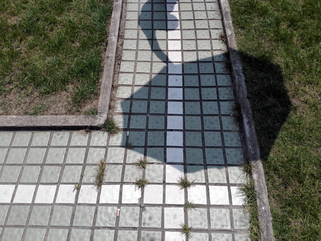
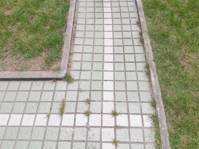
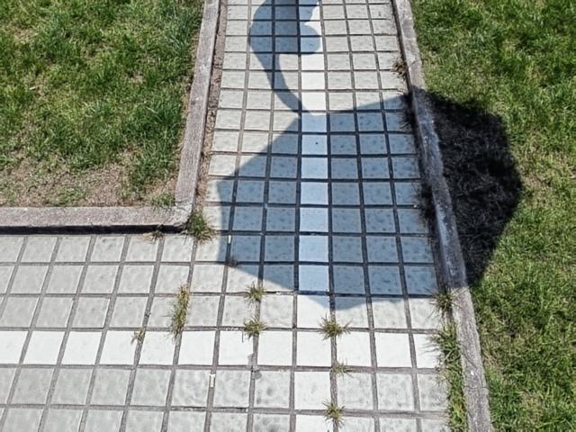
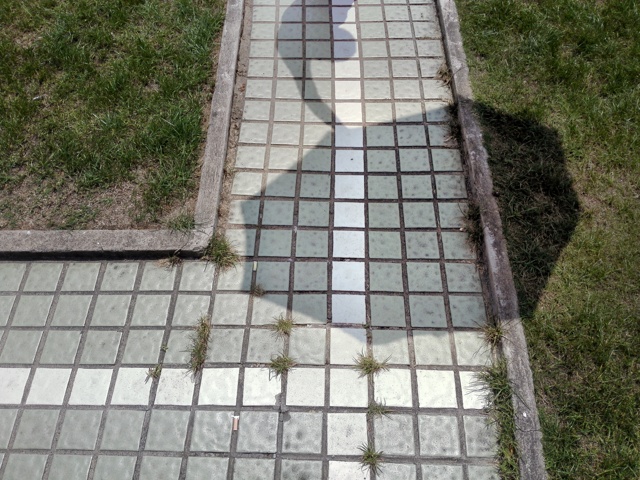
Deep learning-based shadow removal methods can learn the mapping between shadow and shadow-free images from large-scale training data. They are typically based on different network structures and learning strategies (e.g., directional convolution (Hu et al. 2019a), coarse-to-fine strategy (Ding et al. 2019; Wan et al. 2022), GANs (Wang, Li, and Yang 2018; Ding et al. 2019; Cun, Pun, and Shi 2020), and multi-exposure fusion (Fu et al. 2021)) to learn color mapping directly, which may produce color-shifted artifacts (Zhu et al. 2022a). Recent methods (Chen et al. 2021; Jin, Sharma, and Tan 2021; Zhu et al. 2022a) propose to model shadow-invariant color priors by, e.g., averaging the color of the whole image (Chen et al. 2021), using hand-crafted statistics (Jin, Sharma, and Tan 2021), and training an auxiliary network (Zhu et al. 2022a). Nonetheless, as shown in Fig. 1(b-e), although these existing methods may be able to recover the lighting of shadow regions to some extent, they fail to remove shadow remnants in the homogeneous region and to recover the details in the texture region.

In this work, we observe that in a shadow region, the degradation degree of object textures depends on the local illumination, and enhancing only the local illumination alone would not be able to fully recover the attenuated textures. There are two reasons for this. First, shadows may have sharp boundaries that are mixed with object textures and are difficult to be completely recovered simply by enhancing the lighting alone. Second, object textures may appear differently under different illuminations (Serrano et al. 2021). Hence, unlike existing methods that attempt to directly recover the contents of the shadow regions, in this paper, we propose to address this problem in two steps. First, we learn a color-to-illumination mapping, which helps regenerate the lighting in shadow regions. Second, we use the regenerated lighting to guide the texture recovery.

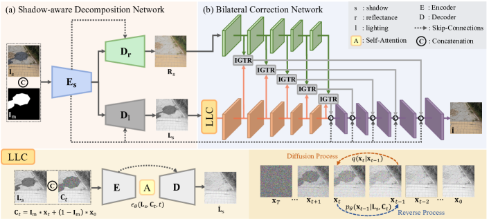
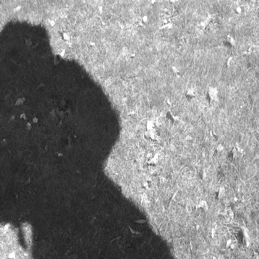
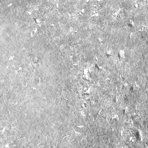
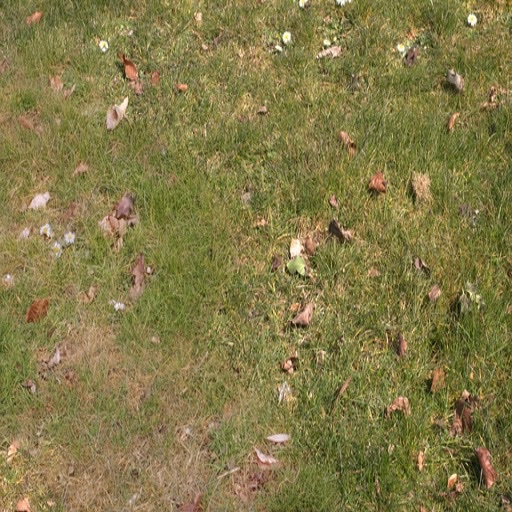
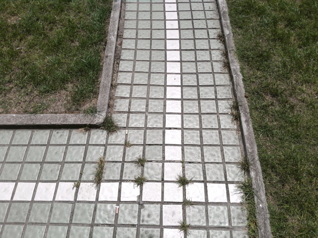
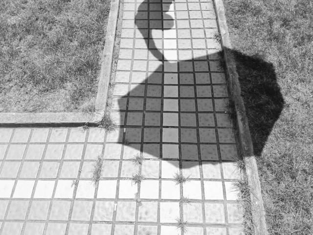
Based on this idea, we propose a novel shadow removal method, which has two parts: (1) a shadow-aware decomposition network that explicitly estimates the illumination and reflectance layers for shadow images; and (2) a novel bilateral correction network that first generates the homogeneous lighting and then recovers the textures in shadow regions conditioned on the generated lighting. We follow the retinex theory (Land 1977) to optimize the shadow-aware decomposition network to ensure a physically-correct illumination estimation (see Fig. 1(f,g), where the shadows are learned to be captured by in the illumination layer only.) Our bilateral correction network has two novel designs: a local lighting correction (LLC) module and an illumination-guided texture restoration (IGTR) module. The former iteratively corrects the local lighting of shadow regions by local conditional denoising, while the latter restores local textures by scale-adaptive feature consistency enhancement. As shown in Fig. 1(h), our method can remove the shadow and produce a more accurate image. In addition, as the widely used Shadow Removal Dataset (SRD) (Qu et al. 2017) does not provide shadow masks, existing removal methods have to use shadow masks of different detection methods. For fair evaluations, we manually annotate the shadow masks for it.

To sum up, we have the following key contributions:

• To remove shadows, we propose to correct degraded textures in shadow regions conditioned on recovered illumination. Our method includes a shadow-aware decomposition network and a novel bilateral correction network.

• We introduce two novel modules for the bilateral correction network: (1) a local lighting correction module that recasts shadow region lighting via local conditional denoising, and (2) an illumination-guided texture restoration module that employs scale-adaptive features to enhance local textures, conditioned on recovered lighting.

• We manually annotate accurate shadow masks for the SRD dataset, to ensure fair evaluation with existing methods, and propel the advancement of this field.

• Extensive experiments on three shadow removal benchmarks demonstrate that (1) our method achieves state-of-the-art performances, and (2) our shadow-aware decomposition method can reduce the input requirement from a pixel-wise mask to a coarse bounding box.

Figure 2: Method Overview. Given a shadow image $\mathbf{I}_{\text{s}}$ and a shadow mask $\mathbf{I}_{\text{m}}$ as input, the proposed method first decomposes the shadow image into a reflectance layer $\mathbf{R}_{\text{s}}$ and an illumination layer $\mathbf{L}_{\text{s}}$ via the shadow-aware decomposition network. $\mathbf{R}_{\text{s}}$, $\mathbf{L}_{\text{s}}$, and image features through skip-connections are then fed into the bilateral correction network for lighting correction via the Local Lighting Correction (LLC) module to generate the shadow-free lighting $\hat{\mathbf{L}}_{\text{s}}$, and texture restoration via the Illumination-Guided Texture Restoration (IGTR) module, and output the prediction $\mathbf{\hat{I}}$. In LLC, t is the time step, $\mathbf{x}_{0}$ is $\mathbf{L}_{\text{s}}$ during inference.

Related Work

Deep Shadow Removal Methods take advantages of large-scale datasets (Qu et al. 2017; Wang, Li, and Yang 2018; Le and Samaras 2021). Some methods focus on designing different network structures, e.g., contexts (Qu et al. 2017; Cun, Pun, and Shi 2020), directions (Hu et al. 2019a), exposures (Fu et al. 2021; Sun et al. 2023), residuals (Zhang et al. 2020a) and structures (Liu et al. 2023b), for shadow removal. Another group of works (Hu et al. 2019b; Le and Samaras 2020; Liu et al. 2021b; Jin, Sharma, and Tan 2021; Liu et al. 2021a; He et al. 2021) propose a variety of learning strategies to train shadow removal networks using unpaired images. Recently, several methods are proposed to model shadow-variant, e.g., SP+M+I (Le and Samaras 2021) and EMNet (Zhu et al. 2022b), and shadow-invariant, e.g., CANet (Chen et al. 2021), DCGAN (Jin, Sharma, and Tan 2021) and BMNet (Zhu et al. 2022a), information to guide the shadow removal process. SP+M+I proposes to estimate a group of linear parameters to represent the illumination information for shadow removal. EMNet further introduces non-linearity into the shadow formation model to predict a pixel-wise shadow degradation map. CANet removes shadows using a shadow-invariant color map obtained by averaging shadow image colors and transferring features between shadow and non-shadow regions. DCGAN uses the shadow-invariant chromaticity map from traditional methods (Drew, Finlayson, and Hordley 2003; Finlayson, Drew, and Lu 2009) as pseudo labels for training. Instead, BMNet directly trains a network to predict a shadow-invariant color map with the supervision of color maps averaged from shadow-free images and uses it to guide the removal process. Unlike existing methods that implicitly process lighting and textures simultaneously, we introduce a two-step approach to estimate and rectify the illumination in shadow regions first, followed by the restoration of degraded textures in these regions, conditioned on the recovered illumination.

Retinex Models (Land 1977), which decompose an image into a reflectance image and an illumination image, provide a theoretical foundation for image formation and decomposition and have been widely used for image intrinsic decomposition (Baslamisli, Le, and Gevers 2018) and low-light enhancement (Wei et al. 2018; Zhang et al. 2021) tasks. They typically design different network structures to estimate both reflection and illumination images, while Wang et al. (Wang et al. 2019) assumes that the reflection image is the normal-light image and focuses on estimating only the enhanced illumination image. However, these methods often fail to model illumination changes between shadow and non-shadow regions as they assume spatially consistent lighting. In our work, we leverage various spatially-variant physical regularizations for modeling the lack of lighting in shadow regions during image decomposition.

Diffusion Models are generative models (Sohl-Dickstein et al. 2015) that learn data distributions by the Gaussian noise blurring process and the reverse denoising process. They have been applied to various tasks, e.g., image super-resolution (Saharia et al. 2022b), image generation (Ho, Jain, and Abbeel 2020; Dhariwal and Nichol 2021) and color harmonization (Xu, Hancke, and Lau 2023). Some works (Rombach et al. 2022; Saharia et al. 2022a; Zhang and Agrawala 2023) propose to use additional inputs, e.g., texts, depth and sketch, as conditions to enable global image generation or editing. In this work, we introduce the diffusion model into shadow removal and exploit its strong generative ability to recast the local lighting of shadow regions conditioned on the global lighting of shadow image.

Proposed Method

Recent deep shadow removal methods typically formulate the task as $\mathbf{\hat{I}}=\phi(\mathbf{I}_{\text{s}}|\mathbf{P})$, where $\phi(\cdot)$ is a pixel-to-pixel color mapping between a shadow image $\mathbf{I}_{\text{s}}$ and a shadow-free image $\mathbf{\hat{I}}$. $\mathbf{P}$ represents the shadow position hints $\mathbf{I}_{\text{m}}$ (e.g., quadmap (Wu et al. 2007) and mask (Le and Samaras 2019)), which may additionally include the shadow invariant color map $\mathbf{I}_{\text{c}}$ (e.g., in (Chen et al. 2021) and (Jin, Sharma, and Tan 2021)). However, such a formulation is not able to recover the degradation of lighting and textures in shadow regions separately. Although often less notable, shadows often have clear boundaries that may disrupt the original textures, and recovering the textures requires correcting the local lighting first. Hence, instead of directly applying the above formula for shadow removal, in this paper, we propose to remove shadows by recasting the local lighting in shadow regions and correcting the textures conditionally.

Our method, depicted in Fig. 2, comprises two primary stages. In the first stage, we present a shadow-aware decomposition network for accurate reflectance-illumination separation. The second stage introduces a bilateral correction network that initially corrects degraded lighting in shadow areas using a local lighting correction module, followed by a progressive recovery of degraded texture details via an illumination-guided texture restoration module, conditioned on the corrected lighting.

Shadow-aware Decomposition Network

Network Architecture. As shown in Fig. 2 (a), the proposed shadow-aware decomposition network consists of a shared encoder ($\mathbf{E}_{\text{s}}$) to extract shadow image features and two functionally distinct decoders ($\mathbf{D}_{\text{r}}$ and $\mathbf{D}_{\text{l}}$) to handle domain-specific reflectance and illumination features. The encoder has five convolutional layers, each of which employs the kernel size, stride, and padding of 4 and 2, and 1, respectively, and is followed by an InstanceNorm and a Leaky-ReLU layer. The decoder contains five transposed convolution layers with the same hyper-parameter settings as the convolutional layer in the encoder, each followed by an InstanceNorm and a ReLU. By default, skip connections are applied to all convolutional layers, where encoder and decoder features are concatenated.  The decomposed reflectance $\mathbf{R}_{\text{s}}$ and illumination $\mathbf{L}_{\text{s}}$ are then normalized to a range of $[0,1]$.

Shadow-aware Decomposition. Optimizing $\mathbf{R}_{\text{s}}$ and $\mathbf{L}_{\text{s}}$ simultaneously is not straightforward, since there are no ground-truth reflectance and illumination in shadow removal. To this end, we design a new self-supervised learning strategy. Specifically, we leverage another network of the same architecture to the shadow-aware decomposition network to predict the reflectance $\mathbf{R}_{\text{sf}}$ and illumination $\mathbf{L}_{\text{sf}}$ of the shadow-free image. We train the two networks jointly with three physically correct self-supervised regularizations to guide the shadow-aware decomposition process.

1) Maintaining Image Fidelity. We first apply a $\mathit{L}_{1}$ loss to ensure that the decomposed layers can be reverted to the original input (either shadow $\mathbf{I}_{\text{s}}$ or shadow-free $\mathbf{I}_{\text{sf}}$):

$$\mathcal{L}_{\text{fid }}=\sum_{i\in\text{\{s,sf\} }}\left\|\mathbf{R}_{i}*\mathbf{L}_{i}-\mathbf{I}_{i}\right\|_{1}\text{. }$$ (1)

2) Pulling Illumination Layers. Although shadows may degrade both illumination and reflectance layers, the major difference between a shadow image and a shadow-free image should be preserved in their illumination layers. Note that ground truth annotations for $\mathbf{R}$ and $\mathbf{L}$ are not available. Hence, we incorporate the Retinex theory (Land 1977) into the illumination separation process by assuming consistent reflectance of shadow/non-shadow images:

$$\mathcal{L}_{\text{ill }}=\left\|\mathbf{R}_{\text{s }}-\mathbf{R}_{\text{sf }}\right\|_{1}+\sum_{i,j\in\text{\{s,sf\} }\text{,}i\neq j}\left\|\mathbf{R}_{i}*\mathbf{L}_{j}-\mathbf{I}_{j}\right\|_{1}\text{, }$$ (2)

where the first term minimizes the differences between the reflectance layers of shadow and shadow-free images (i.e., $\mathbf{R}_{\text{s}}$ and $\mathbf{R}_{\text{sf}}$), and the second term implicitly minimizes the illumination difference of non-shadow regions between the shadow and shadow-free images (i.e., $\mathbf{L}_{\text{s}}$ and $\mathbf{L}_{\text{sf}}$).

3) Constraints on Reflectance Layers. Last, we apply the gradient constraints (Meka et al. 2021) on the reflectance layers to ensure texture preservation and color correction:

$$\mathcal{L}_{\text{ref }}=\sum_{i\in\text{ \{s,sf\} }}\left\|\nabla\mathbf{L}_{\text{sf}}*\exp\left(\lambda_{n}\nabla\mathbf{R}_{i}\right)\right\|_{1}\text{,}$$ (3)

$$\mathit{s.t.}\quad 0\leq\mathbf{R}_{i}<\mathbf{L}_{\text{sf}}\leq 1$$

where $\lambda_{\text{n}}$ is a hyper-parameter to adjust the weight of the gradients of reflectance layers and is set to $-20$. Note that we do not involve $\mathbf{L}_{\text{s}}$ in Eq. 3, to avoid the illumination layer degrading into a shadow matte (Qu et al. 2017) and the reflectance layer being identical to the input shadow image.

The whole shadow-aware decomposition process is supervised by the following loss function:

$$\mathcal{L}_{\text{de}}=\mathcal{L}_{\text{fid}}+\mathcal{L}_{\text{ill}}+w_{\text{r}}\mathcal{L}_{\text{ref}}\text{, }$$ (4)

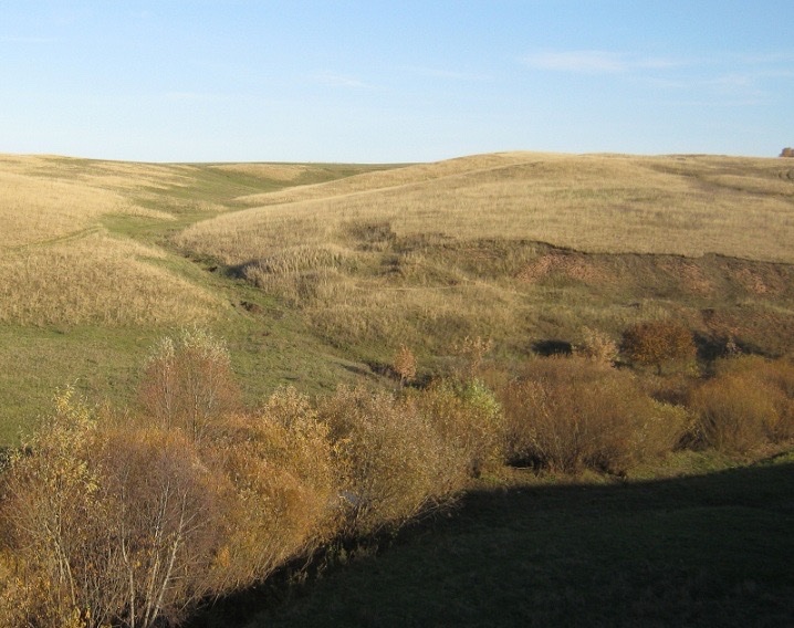
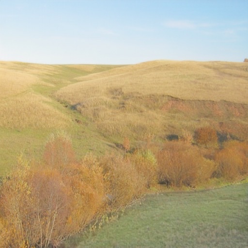
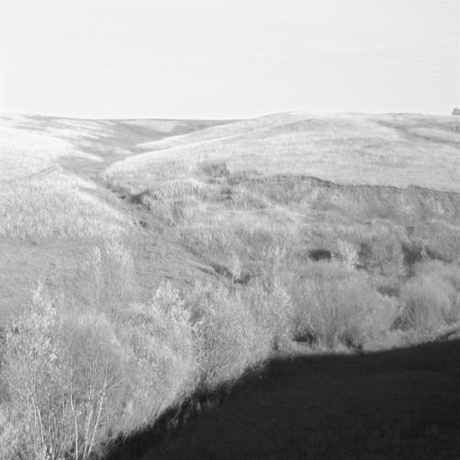
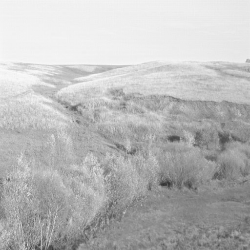
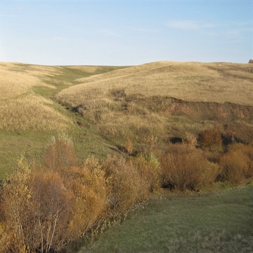
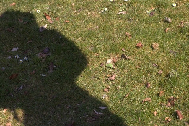
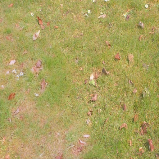
where $w_{\text{r}}$ is balancing parameter and empirically set to 0.1. See Fig. 3 for our shadow-aware decomposition illustration.

(a) $\mathbf{I}_{\text{s}}$	(b) $\mathbf{R}_{\text{s}}$	(c) $\mathbf{L}_{\text{s}}$	(d) $\hat{\mathbf{L}}_{\text{s}}$	(e) $\hat{\mathbf{I}}_{\text{s}}$

Figure 3: Two examples of our shadow-aware decomposition and final prediction results in real-world samples.

Bilateral Correction Network

With decomposed illumination $\mathbf{L}_{\text{s}}$ and reflectance $\mathbf{R}_{\text{s}}$, we first recast regional lighting via the proposed local lighting correction (LLC) module to produce a homogeneous illumination layer. We then extract cross-level features of the reflectance and re-casted illumination via an encoder, and apply the proposed illumination-guided texture restoration (IGTR) module at multiple scales to enhance their feature consistency and progressively restore local textures.

Local Lighting Correction. Since local illumination of an image is sample-specific and spatially non-uniform (Zhu et al. 2022b), learning a fixed set of parameters for all samples through a regression-based network is typically insufficient and inaccurate. To solve such a problem, we consider local lighting correction as a generation problem and resort to the diffusion model to recast the lighting iteratively.

However, we note that DDPM is essentially a global denoising process, which is not able to focus on the local shadow regions of our task. Hence, we formulate our local lighting correction module based on the DDPM with two conditions: the independent shadow lighting condition $\mathbf{L}_{s}$ and the time-embedded non-shadow lighting condition $\mathbf{C}_{t}$. The former focuses our module on the local lighting of shadow regions, while the latter provides globally-consistent lighting guidance for the local light generation:

$$\mathbf{C}_{t}=\mathbf{I}_{\text{m}}*\mathbf{x}_{t}+\left(\mathbf{1}-\mathbf{I}_{\text{m}}\right)*\mathbf{x}_{0}\text{,}$$ (5)

where $t$ is the time step, $\mathbf{x}_{t}=\left(\sqrt{\bar{\alpha}_{t}}\mathbf{x}_{0}+\sqrt{1-\bar{\alpha}_{t}}\boldsymbol{\epsilon}_{t}\right)$ in which $\bar{\alpha}$ is the variance schedule, and $\boldsymbol{\epsilon}$ is the randomly sampled gaussian noise. $\mathbf{1}$ is a mask filled with 1. During training, we set $\mathbf{x}_{0}$ to $\mathbf{L}_{\text{sf}}$ and feed the conditions and $t$ to the noise prediction network $\boldsymbol{\epsilon}_{\theta}\left(\cdot\right)$ to conduct local conditional noise prediction and update its parameters. During testing, we set $\mathbf{x}_{0}$ to $\mathbf{L}_{\text{s}}$ and perform the iterative local conditional denoising to generate the $\hat{\mathbf{L}}_{\text{s}}$. We adopt an improved UNet (Dhariwal and Nichol 2021) as our noise prediction network $\boldsymbol{\epsilon}_{\theta}(\cdot)$, and train it using the MSE denoising loss within the shadow regions, as:

$$\mathcal{L}_{\mathrm{denoise}}=\mathbb{E}_{\boldsymbol{\epsilon}\sim\mathcal{N}(\mathbf{0},\mathbf{I})}\left[\mathbf{I}_{\text{m}}*\left\|\boldsymbol{\epsilon}-\boldsymbol{\epsilon}_{\theta}\left(\mathbf{C}_{t}\text{,}\;\mathbf{L}_{\text{s}}\text{,}\;t\right)\right\|_{2}^{2}\right]\text{.}$$ (6)

In this way, the diffusion model can focus on the shadow regions conveniently and exploit the correct illumination of the non-shadow regions. Refer to the comparison between the 3rd and 4th columns in Fig. 3 for an visual illustration.

Figure 4: Overview of the proposed Illumination-Guided Texture Restoration (IGTR) module. It aims to correct the textures with the guidance of the recovered local lighting.

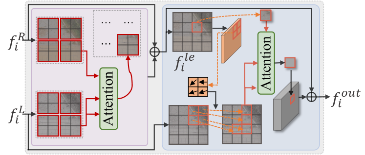
Illumination-Guided Texture Restoration. With the re-generated illumination $\hat{\mathbf{L}}_{\text{S}}$, we propose to condition the local texture restoration on the recovered local lighting, with two kinds of lighting-to-texture correspondences being modeled for texture fidelity. We first correct each local region of the reflectance layer according to the lighting of the corresponding local region in the illumination layer. Then, we enhance the texture consistency by learning the correspondence between each local reflectance token and adjacent regions in the illumination layer.

Fig. 4 shows the overview of the proposed IGTR module. Formally, given the features of reflectance and corrected illumination at scale $i\in\{1\text{,}2\text{,}\cdots\text{,}5\}$ as $f^{\text{R}}_{i}\in R^{H_{i}\times W_{i}\times C_{i}}$ and $f^{\text{L}}_{i}\in R^{H_{i}\times W_{i}\times C_{i}}$ (where $H$, $W$ and $C$ represent height, width, and channel), we first divide them into local regions of size $K_{i}\times K_{i}$. We then compute the local lighting-to-texture correspondence between each corresponding region in $f^{\text{R}}_{i}$ and $f^{\text{L}}_{i}$ via co-attention (CoA) (Vaswani et al. 2017):

$$\text{CoA}(f^{\text{R}}_{i}\text{, }f^{\text{L}}_{i})=\mathcal{S}\left((\text{W}_{q}f^{\text{R}}_{i})(\text{W}_{k}{f^{\text{L}}_{i}})^{T}/\sqrt{\text{d}}\right)(\text{W}_{v}f^{\text{L}}_{i})\text{,}$$ (7)

where d and $\mathcal{S}$ are the scaling factor and SoftMax operation, and $\text{W}_{j}\text{, }j\in\{\text{q}\text{, }\text{k}\text{, }\text{v}\}$ is projection function (conv. layer) to reduce the feature dimension by half. We then obtain the enhanced texture features $f^{\text{le}}_{i}=\text{CoA}(f^{\text{R}}_{i}\text{, }f^{\text{L}}_{i})+f^{\text{R}}_{i}$.

We further build the non-local lighting-to-texture correspondence between each token in $f^{\text{R}}_{i}$ and the neighbouring regions in $f^{\text{L}}_{i}$, where the adjacent regions in $f^{\text{L}}_{i}$ are adaptively searched based on enhanced texture features $f^{\text{le}}_{i}$:

$$\hat{f}^{\text{L}}_{i}=\mathcal{B}(f^{\text{L}}_{i}\text{,}\;\mathbf{Shift}(f^{\text{le}}_{i}))\text{,}$$ (8)

where $\mathbf{Shift}$ is a shifting network (Xia et al. 2022) to learn offsets for each location in the local region, and $\mathcal{B}(\cdot)$ is the bilinear interpolation for feature-resampling. We then obtain the final enhanced texture feature: $f^{\text{out}}_{i}=\text{CoA}(f^{\text{le}}_{i}\text{,}\hat{f}^{\text{L}}_{i})+f^{\text{le}}_{i}$.

Loss Functions. We adopt the L1 loss and the perceptual loss (Johnson, Alahi, and Fei-Fei 2016) for training the texture restoration process, as:

$$\mathcal{L}_{\text{re }}=\left\|\mathbf{\hat{I}}\text{, }\mathbf{I}_{\text{sf}}\right\|_{1}+\lambda_{\text{vgg}}*\left\|\text{VGG}(\mathbf{\hat{I}})\text{, }\text{VGG}(\mathbf{I}_{\text{sf}})\right\|_{1}\text{. }$$ (9)

where $\lambda_{\text{vgg}}$ is empirically set to 0.1 to maintain the same gradient magnitude of the two loss items.

Ground Truth Labeling on SRD

SRD (Qu et al. 2017), the inaugural large-scale dataset for shadow removal, doesn’t offer ground truth shadow masks. Hence, extant removal techniques employ various methods like shadow detector (Zhu et al. 2022a), Otsu’s algorithm and morphology (Fu et al. 2021), or shadow matting with threshholding (Cun, Pun, and Shi 2020) to generate shadow masks. Table 1 assesses the accuracy of these shadow masks against our labeled masks as ground truth, using shadow detection metrics (PER and BER (Zhu et al. 2021)). It uncovers considerable quality variations, often rendering evaluations of shadow removal methods on the SRD biased and potentially impacting removal performance (Zhu et al. 2022a). Thus, to ensure a fair evaluation on this dataset, we manually annotate the pixel-wise shadow masks for the SRD dataset.

Metrics	MTMT	DHAN	FDR	AEF
PER $\downarrow$	20.35	20.80	15.03	12.03
BER $\downarrow$	11.81	10.87	10.19	6.49

Table 1: Existing shadow mask quality varies significantly when assessed against our labeled masks as ground truth, with lower PER and BER values indicating higher quality.

Experiments

Implementation Details. Our method is implemented via the PyTorch Toolbox on a single NVIDIA TESLA V100 GPU with 32G memory, is optimized using the Adam (Kingma and Ba 2015) optimizer. The initial learning rate, $\beta_{1}$, $\beta_{2}$, and batch size being set to 0.0002, 0.9, 0.999, and 12. Learning rate adjustment utilizes a warmup and cosine decay strategy. For the local diffusion process, we set the times steps $T$, initial and end variance scheduler $\beta_{\text{t}}$ to $\{1000\text{,}0.0001\text{,}0.02\}$ and $\{50\text{,}0.0001\text{,}0.5\}$ for training and testing. Data is augmented by random flipping and cropping, and resized to 256$\times$256 for training. Shadow-aware decomposition and bilateral correction networks are trained for 100k and 200k iterations, respectively.

Datasets. We conduct experiments on three shadow removal datasets, i.e., SRD (Qu et al. 2017), ISTD (Wang, Li, and Yang 2018), and ISTD+ (Le and Samaras 2021). SRD consists of 3,088 paired shadow and shadow-free images, which are split into 2680 for training and 408 for testing. ISTD contains 1,870 shadow images, shadow masks, and shadow-free image triplets, of which 1,330 are used for training and 540 for testing. ISTD+ further corrects the color inconsistency problem of images from the ISTD.

Evaluation Metrics. We follow (Le and Samaras 2021) to compute the root mean square error (RMSE) between the results and ground truth shadow-free images in the LAB color space, and report the peak signal-to-noise ratio (PSNR) and structural similarity (SSIM) for comparisons. All metrics are computed based on the 256 resolution.

Methods	RMSE $\downarrow$			PSNR $\uparrow$			SSIM $\uparrow$
	S	NS	All	S	NS	All	S	NS	All
DSC	17.25	16.58	16.76	26.71	24.70	21.63	0.914	0.756	0.657
DHAN	7.53	3.55	4.61	33.81	35.02	30.74	0.979	0.982	0.958
AEF	8.13	5.57	6.25	33.26	30.39	27.96	0.970	0.938	0.902
DCGAN	8.03	3.82	4.94	33.36	34.87	30.56	0.973	0.980	0.947
EMNet	9.55	6.67	7.43	30.24	26.32	24.16	0.940	0.851	0.779
BMNet	7.11	3.11	4.18	34.82	36.54	31.97	0.981	0.986	0.965
SGNet	7.45	3.05	4.23	33.76	36.48	31.39	0.979	0.984	0.960
Ours	5.49	3.00	3.66	36.51	37.71	33.48	0.983	0.986	0.967

Table 2: Quantitative comparisons with state-of-the-art shadow removal methods on the SRD dataset. All methods are tested using our manually annotated shadow masks. The best results are marked in bold. S, NS, and ALL indicate the shadow regions, non-shadow regions, and the whole image.

Methods	RMSE $\downarrow$			PSNR $\uparrow$			SSIM $\uparrow$
	S	NS	All	S	NS	All	S	NS	All
ST	9.99	6.05	6.65	33.74	29.51	27.44	0.981	0.958	0.929
DSC	8.72	5.04	5.59	34.64	31.26	29.00	0.984	0.969	0.944
DHAN	8.26	5.56	6.37	34.65	29.81	28.15	0.983	0.937	0.913
DCGAN	11.43	5.81	6.57	31.69	28.99	26.38	0.976	0.958	0.922
G2R	10.72	7.55	7.85	31.63	26.19	24.72	0.975	0.967	0.932
AEF	7.91	5.51	5.88	34.71	28.61	27.19	0.975	0.880	0.945
EMNet	7.78	4.72	5.22	36.27	31.85	29.98	0.986	0.965	0.944
BMNet	7.60	4.59	5.02	35.61	32.80	30.28	0.988	0.976	0.959
Ours	6.54	3.40	3.91	36.61	35.75	32.42	0.988	0.979	0.961

Table 3: Quantitative comparisons with state-of-the-art shadow removal methods on the ISTD dataset.

Methods	RMSE $\downarrow$			PSNR $\uparrow$			SSIM $\uparrow$
	S	NS	All	S	NS	All	S	NS	All
P+M+D	9.67	2.82	3.94	33.09	35.35	30.15	0.983	0.978	0.951
DCGAN	10.41	3.63	4.74	32.00	33.56	28.77	0.976	0.968	0.932
G2R	7.35	2.91	3.64	35.78	35.64	31.93	0.987	0.977	0.957
AEF	6.55	3.77	4.22	36.04	31.16	29.45	0.978	0.892	0.861
SP+M+I	5.91	2.99	3.46	37.60	36.02	32.94	0.990	0.976	0.962
BMNet	6.10	2.90	3.50	37.30	37.93	33.95	0.990	0.981	0.965
SGNet	5.93	2.92	3.41	36.79	35.57	32.45	0.990	0.977	0.962
Ours	5.69	2.31	2.87	38.04	39.15	34.96	0.990	0.984	0.968

Table 4: Quantitative comparison with state-of-the-art shadow removal methods on the ISTD+ dataset.

Input Shadow	DC-GAN	DHAN	AEF	G2R	SGNet	BMNet	Ours

Figure 5: Visual comparisons with state-of-the-art shadow removal methods on real-world samples.

Comparing to State-of-the-arts

We compare our method with twelve shadow removal methods: ST-CGAN (Wang, Li, and Yang 2018), DSC (Hu et al. 2019a), DHAN (Cun, Pun, and Shi 2020), P+M+D (Le and Samaras 2020), DCGAN (Jin, Sharma, and Tan 2021), SP+M+I (Le and Samaras 2021), G2R (Liu et al. 2021b), AEF (Fu et al. 2021), EMNet (Zhu et al. 2022b), BMNet (Zhu et al. 2022a) and SGNet (Wan et al. 2022).

For SRD (Table 2), our method considerably surpasses other methods, even beating the latest color mapping-based method SGNet (Wan et al. 2022) and shadow-invariant map-based method BMNet (Zhu et al. 2022a) by 26.3$\%$ and 22.8$\%$ in RMSE for shadow regions, respectively. When assessed on ISTD and ISTD+ (Table 3 and 4), our method again outperforms, achieving a 13.9$\%$ and 6.7$\%$ decrease in RMSE for shadow regions compared to BMNet (Zhu et al. 2022a). As shown in Fig. 5, visual comparisons on real-world samples also illustrate our method’s proficiency in reducing shadow ghosting (row-1), maintaining color consistency (row-2), and correcting textures (row-3 and 4) after shadow removal, particularly in challenging scenarios with homogenous colors or textured scenes.

Internal Analysis

In & GT	Ours	EMNet	RetinexNet	DeepUPE

Figure 6: Visual comparisons of decomposition results among our method, shadow removal method EMNet, and two retinex-based low-light enhancement methods RetinexNet (Wei et al. 2018) and DeepUPE (Wang et al. 2019) re-trained using shadow masks as additional input.

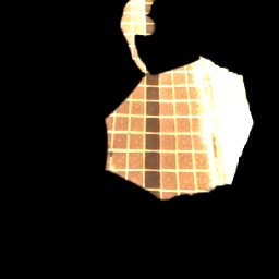
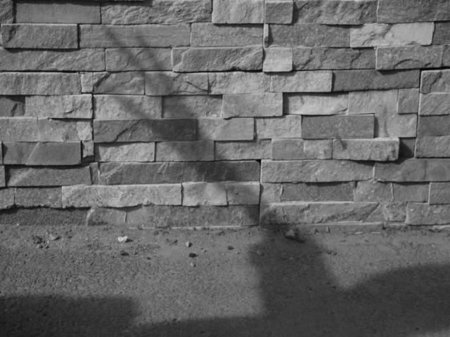
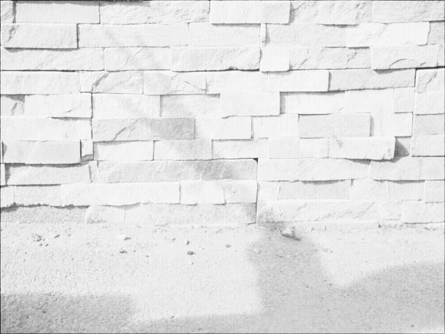
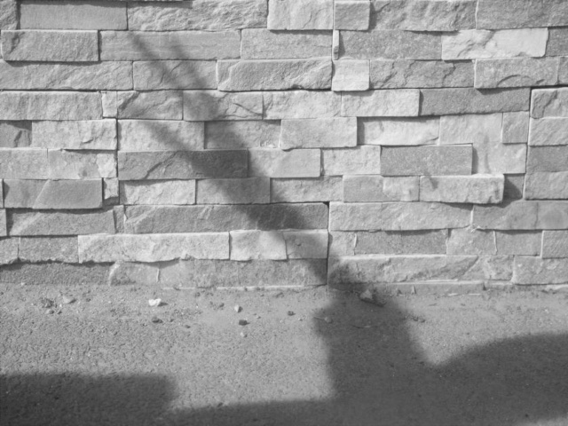
Shadow-aware Decomposition Evaluation. We illustrate the correctness of our shadow-aware decomposition by visually comparing it to related methods, as there is no ground truth for quantitative evaluation. Fig. 6 compares ours to the shadow formation-based EMNet and two retinex-based methods, DeepUPE (Wang et al. 2019) and RetinexNet (Wei et al. 2018). The degradation map of EMNet jointly models the lighting and reflectance, resulting in the pinkish remnants in their shadow-free image. On the other hand, the two retinex-based methods fail to separate the reflectance and illumination layers due to their spatially invariant property. In contrast, our spatially-variant regularizations ensure the physically correct shadow decomposition.

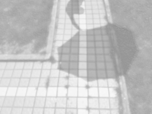
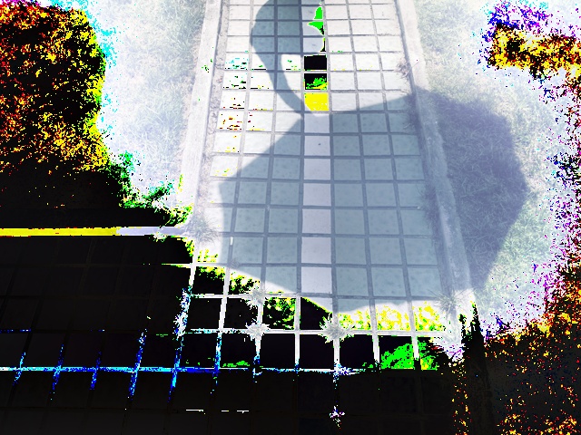
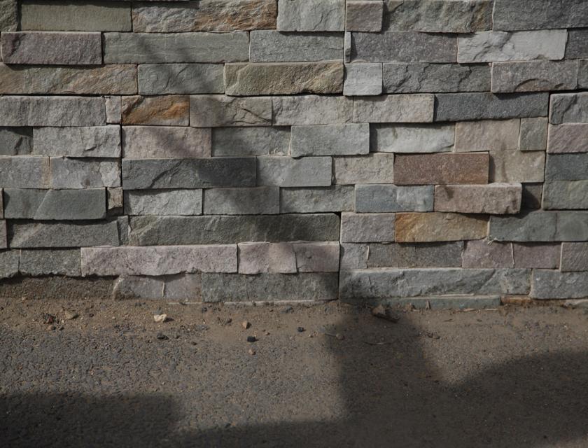
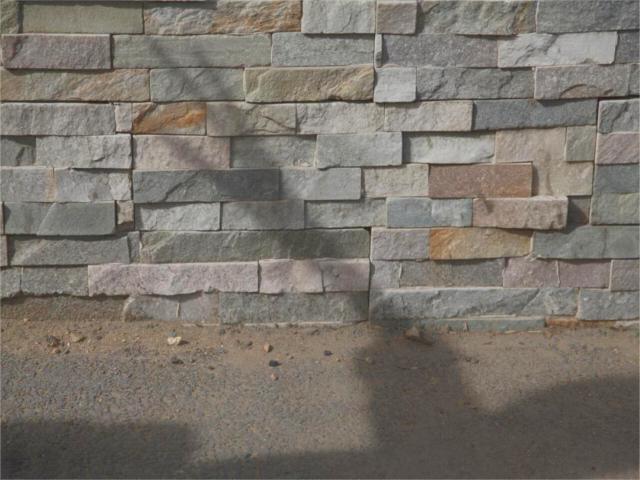
Fig. 7 shows visual comparisons of various regularizations. Shadows persist in both $\mathbf{R}_{\text{s}}$ and $\mathbf{L}_{\text{s}}$ when relying solely on $\mathcal{L}_{\text{fid}}$. Despite the separation of $\mathbf{R}_{\text{s}}$ and $\mathbf{L}_{\text{s}}$ when $\mathcal{L}_{\text{ill}}$ is added to $\mathcal{L}_{\text{fid}}$, $\mathbf{R}_{\text{s}}$ shows poor color quality due to inadequate regularization. Combining $\mathcal{L}_{\text{fid}}$ and $\mathcal{L}_{\text{ref}}$ produces similar results to those of $\mathcal{L}_{\text{fid}}$. Finally, the $\mathcal{L}_{\text{de}}$ demonstrates the indispensability of all regularizations to the final decomposition.

Input $\&$ GT	$\mathcal{L}_{\text{fid}}$	$\mathcal{L}_{\text{fid}}+\mathcal{L}_{\text{ill}}$	$\mathcal{L}_{\text{fid}}+\mathcal{L}_{\text{ref}}$	$\mathcal{L}_{\text{de}}$

Figure 7: Visual comparisons of shadow decomposition of our method with different regularizations.

	Type of condition			Range of denoising		S
	[$\mathbf{L}_{\text{s}}$]	[$\mathbf{L}_{\text{s}}\text{,}\mathbf{I}_{\text{m}}$]	[$\mathbf{L}_{\text{s}}\text{,}\mathbf{C}_{t}$]	Local	Global	RMSE $\downarrow$	PSNR $\uparrow$
(a)	✓				✓	10.43	31.55
(b)	✓			✓		9.40	32.44
(c)		✓			✓	10.19	31.92
(d)		✓		✓		8.57	33.62
Ours			✓	✓		6.54	36.61

Table 5: Ablation study of the proposed LLC on the ISTD dataset. Local and Global refer to the mask regions and whole image. For simplicity, we omit the time step $t$ in [$\cdot$].

Local Lighting Correction Evaluation. In Table 5, we compare our LLC with four variants to evaluate its effectiveness. In (a) and (b), we train global and local diffusion process with only $\mathbf{L}_{s}$ as conditional input, respectively. In (c) and (d), we add the $\mathbf{I}_{\text{m}}$ as another input condition to indicate the shadow regions. The results demonstrate that: (1) conducting denoising process locally rather than globally can achieve better performance (see (a)/(b) or (c)/(d)), as the spatially uniform noise distribution assumed by the global diffusion may not handle differences of intensity distributions between shadow and non-shadow regions; (2) the comparisons of Ours to (b) and (d) prove that the lighting prior from non-shadow regions is crucial for shadow region illumination correction, as it uses global lighting information to efficiently constrain the sampling space in diffusion process; (3) explicitly using the lighting prior from non-shadow regions as a time-embedded condition provides further significant performance improvement (see (d) and Ours).

Illumination-guided texture restoration Evaluation. We further evaluate our IGTR module with six variants in Table 6. First, we directly composing $\mathbf{R}_{\text{s}}$ and $\hat{\mathbf{L}}_{\text{s}}$ via element-wise multiplication, referred to as “$\mathbf{R}_{\text{s}}\times\hat{\mathbf{L}}_{\text{s}}$”. Second, we exclude IGTR and concatenate $\mathbf{R}_{\text{s}}$ and $\hat{\mathbf{L}}_{\text{s}}$, or their corresponding features, resulting in two baselines: “Cat (i)” and “Cat (f)”. Next, we substitute IGTR with the standard self-attention (Vaswani et al. 2017), labeled as “SA”. Finally, we remove the local and non-local lighting-to-texture correspondence modeling in the IGTR, separately, yielding “IGTR (L)” and “IGTR (G)”.

Table 6 indicates that omitting IGTR compromises shadow removal efficacy, with our IGTR outperforming the standard self-attention. It also demonstrates that both local and non-local lighting-to-texture correspondence modeling aids in restoring shadow region textures, and their combination optimizes results. Further, comparing Cat(i) and Cat(f), SA and/or IGTR(G) with IGTR(L) highlights the superior utility of local-based features over global-based ones.

S	$\mathbf{R}_{\text{s}}\times\hat{\mathbf{L}}_{\text{s}}$	Cat (i)	Cat (f)	SA	IGTR (G)	IGTR (L)	Ours
RMSE $\downarrow$	7.37	7.30	7.20	7.32	7.27	7.00	6.54

Table 6: Ablation study of the proposed IGTR on the ISTD dataset. Cat (i) and (f) mean that the $\mathbf{R}_{\text{s}}$ and $\hat{\mathbf{L}}_{\text{s}}$ are concatenated at the input and feature-level. SA denotes the standard self-attention. IGTR (G) and (L) refer to the non-local and local lighting-to-texture corresponding.

Datasets	Bounding boxes		Dilation masks		GT masks
	RMSE$\downarrow$	PSNR$\uparrow$	RMSE$\downarrow$	PSNR$\uparrow$	RMSE$\downarrow$	PSNR$\uparrow$
SRD	5.69	36.39	5.49	36.51	5.40	36.79
ISTD	6.70	35.97	6.54	36.61	5.98	37.65
ISTD+	5.82	37.77	5.69	38.04	5.63	38.34

Table 7: Our method is robust to different types of shadow annotations. Metrics are evaluated in the shadow regions.

Methods	G2R	AEF	SP+M+I	SGNet	Ours
Params. (MB)	27.75	143.01	195.6	6.2	171.87
Time (s)	0.32	0.14	0.15	0.25	1.70

Table 8: Comparisons of parameters and inference time.

Robustness to Shadow Annotations. In Table 7, we compare the shadow removal results using our method with bounding boxes, dilated (Fu et al. 2021), and ground truth masks. Benefiting from the proposed shadow-aware decomposition that constrains shadows to illumination layer, our method is robust to the accuracy of shadow masks. Notably, our method using bounding box outperforms the BMNet using shadow mask with 11.8% RMSE reduction in the shadow regions on the ISTD dataset.

Conclusion

In this paper, we have proposed a novel method for shadow removal, which includes a shadow-aware decomposition network to derive the shadow reflectance and illumination layers. A novel bilateral correction network is proposed with a novel LLC module and a novel IGTR module, to re-cast the degraded lighting and restore the degraded textures in shadow regions conditionally. We have also annotated the shadow masks for the SRD benchmark, for a fair evaluation with existing shadow removal methods. We conduct extensive experiments on three shadow removal benchmarks, to demonstrate the superior performance of our method.

Despite its efficacy, our method has limitations, including slightly larger parameters and extended inference times due to the use of diffusion, as shown in Tab 8. For instance, our method requires 1.7 seconds to process a 640 $\times$ 480 image.

References

- Baslamisli, Le, and Gevers (2018) Baslamisli, A. S.; Le, H.-A.; and Gevers, T. 2018. CNN based learning using reflection and retinex models for intrinsic image decomposition. In CVPR.
- Brown and Tsoi (2006) Brown, M. S.; and Tsoi, Y.-C. 2006. Geometric and shading correction for images of printed materials using boundary. IEEE TIP.
- Chen et al. (2021) Chen, Z.; Long, C.; Zhang, L.; and Xiao, C. 2021. CANet: A Context-Aware Network for Shadow Removal. In ICCV.
- Cun, Pun, and Shi (2020) Cun, X.; Pun, C.-M.; and Shi, C. 2020. Towards ghost-free shadow removal via dual hierarchical aggregation network and shadow matting GAN. In AAAI.
- Dhariwal and Nichol (2021) Dhariwal, P.; and Nichol, A. 2021. Diffusion models beat gans on image synthesis. In NeurIPS.
- Ding et al. (2019) Ding, B.; Long, C.; Zhang, L.; and Xiao, C. 2019. Argan: Attentive recurrent generative adversarial network for shadow detection and removal. In ICCV.
- Drew, Finlayson, and Hordley (2003) Drew, M. S.; Finlayson, G. D.; and Hordley, S. D. 2003. Recovery of chromaticity image free from shadows via illumination invariance. In ICCVW.
- Finlayson and Drew (2001) Finlayson, G. D.; and Drew, M. S. 2001. 4-sensor camera calibration for image representation invariant to shading, shadows, lighting, and specularities. In ICCV.
- Finlayson, Drew, and Lu (2009) Finlayson, G. D.; Drew, M. S.; and Lu, C. 2009. Entropy minimization for shadow removal. IJCV.
- Finlayson, Hordley, and Drew (2002) Finlayson, G. D.; Hordley, S. D.; and Drew, M. S. 2002. Removing shadows from images using retinex. In CI.
- Finlayson et al. (2005) Finlayson, G. D.; Hordley, S. D.; Lu, C.; and Drew, M. S. 2005. On the removal of shadows from images. IEEE TPAMI.
- Fu et al. (2021) Fu, L.; Zhou, C.; Guo, Q.; Juefei-Xu, F.; Yu, H.; Feng, W.; Liu, Y.; and Wang, S. 2021. Auto-exposure fusion for single-image shadow removal. In CVPR.
- Gryka, Terry, and Brostow (2015) Gryka, M.; Terry, M.; and Brostow, G. J. 2015. Learning to remove soft shadows. ACM TOG.
- Guo, Dai, and Hoiem (2012) Guo, R.; Dai, Q.; and Hoiem, D. 2012. Paired regions for shadow detection and removal. IEEE TPAMI.
- He et al. (2021) He, Y.; Xing, Y.; Zhang, T.; and Chen, Q. 2021. Unsupervised Portrait Shadow Removal via Generative Priors. In ACM MM.
- Ho, Jain, and Abbeel (2020) Ho, J.; Jain, A.; and Abbeel, P. 2020. Denoising diffusion probabilistic models. In NeurIPS.
- Hu et al. (2019a) Hu, X.; Fu, C.-W.; Zhu, L.; Qin, J.; and Heng, P.-A. 2019a. Direction-aware spatial context features for shadow detection and removal. IEEE TPAMI.
- Hu et al. (2019b) Hu, X.; Jiang, Y.; Fu, C.-W.; and Heng, P.-A. 2019b. Mask-ShadowGAN: Learning to remove shadows from unpaired data. In ICCV.
- Jin, Sharma, and Tan (2021) Jin, Y.; Sharma, A.; and Tan, R. T. 2021. DC-ShadowNet: Single-Image Hard and Soft Shadow Removal Using Unsupervised Domain-Classifier Guided Network. In ICCV.
- Johnson, Alahi, and Fei-Fei (2016) Johnson, J.; Alahi, A.; and Fei-Fei, L. 2016. Perceptual losses for real-time style transfer and super-resolution. In ECCV.
- Khan et al. (2015) Khan, S. H.; Bennamoun, M.; Sohel, F.; and Togneri, R. 2015. Automatic shadow detection and removal from a single image. IEEE TPAMI.
- Kingma and Ba (2015) Kingma, D. P.; and Ba, J. 2015. Adam: A Method for Stochastic Optimization. In ICLR.
- Land (1977) Land, E. H. 1977. The retinex theory of color vision. Scientific American.
- Le and Samaras (2019) Le, H.; and Samaras, D. 2019. Shadow removal via shadow image decomposition. In ICCV.
- Le and Samaras (2020) Le, H.; and Samaras, D. 2020. From shadow segmentation to shadow removal. In ECCV.
- Le and Samaras (2021) Le, H.; and Samaras, D. 2021. Physics-based shadow image decomposition for shadow removal. IEEE TPAMI.
- Liu et al. (2023a) Liu, F.; Liu, Y.; Kong, Y.; Xu, K.; Zhang, L.; Yin, B.; Hancke, G.; and Lau, R. 2023a. Referring image segmentation using text supervision. In ICCV, 22124–22134.
- Liu et al. (2023b) Liu, Y.; Guo, Q.; Fu, L.; Ke, Z.; Xu, K.; Feng, W.; Tsang, I. W.; and Lau, R. W. 2023b. Structure-Informed Shadow Removal Networks. IEEE TIP.
- Liu et al. (2021a) Liu, Z.; Yin, H.; Mi, Y.; Pu, M.; and Wang, S. 2021a. Shadow removal by a lightness-guided network with training on unpaired data. IEEE TIP.
- Liu et al. (2021b) Liu, Z.; Yin, H.; Wu, X.; Wu, Z.; Mi, Y.; and Wang, S. 2021b. From Shadow Generation to Shadow Removal. In CVPR.
- Mei et al. (2021) Mei, H.; Ji, G.-P.; Wei, Z.; Yang, X.; Wei, X.; and Fan, D.-P. 2021. Camouflaged object segmentation with distraction mining. In CVPR.
- Meka et al. (2021) Meka, A.; Shafiei, M.; Zollhöfer, M.; Richardt, C.; and Theobalt, C. 2021. Real-time global illumination decomposition of videos. ACM TOG.
- Qu et al. (2017) Qu, L.; Tian, J.; He, S.; Tang, Y.; and Lau, R. W. 2017. Deshadownet: A multi-context embedding deep network for shadow removal. In CVPR.
- Rombach et al. (2022) Rombach, R.; Blattmann, A.; Lorenz, D.; Esser, P.; and Ommer, B. 2022. High-resolution image synthesis with latent diffusion models. In CVPR.
- Saharia et al. (2022a) Saharia, C.; Chan, W.; Chang, H.; Lee, C.; Ho, J.; Salimans, T.; Fleet, D.; and Norouzi, M. 2022a. Palette: Image-to-image diffusion models. In SIGGRAPH.
- Saharia et al. (2022b) Saharia, C.; Ho, J.; Chan, W.; Salimans, T.; Fleet, D. J.; and Norouzi, M. 2022b. Image super-resolution via iterative refinement. IEEE TPAMI.
- Serrano et al. (2021) Serrano, A.; Chen, B.; Wang, C.; Piovarči, M.; Seidel, H.-P.; Didyk, P.; and Myszkowski, K. 2021. The effect of shape and illumination on material perception: model and applications. ACM TOG.
- Sohl-Dickstein et al. (2015) Sohl-Dickstein, J.; Weiss, E.; Maheswaranathan, N.; and Ganguli, S. 2015. Deep unsupervised learning using nonequilibrium thermodynamics. In ICML.
- Sun et al. (2023) Sun, J.; Xu, K.; Pang, Y.; Zhang, L.; Lu, H.; Hancke, G.; and Lau, R. 2023. Adaptive Illumination Mapping for Shadow Detection in Raw Images. In ICCV.
- Vaswani et al. (2017) Vaswani, A.; Shazeer, N.; Parmar, N.; Uszkoreit, J.; Jones, L.; Gomez, A. N.; Kaiser, Ł.; and Polosukhin, I. 2017. Attention is all you need. In NeurIPS.
- Wan et al. (2022) Wan, J.; Yin, H.; Wu, Z.; Wu, X.; Liu, Y.; and Wang, S. 2022. Style-Guided Shadow Removal. In ECCV.
- Wang, Li, and Yang (2018) Wang, J.; Li, X.; and Yang, J. 2018. Stacked conditional generative adversarial networks for jointly learning shadow detection and shadow removal. In CVPR.
- Wang et al. (2019) Wang, R.; Zhang, Q.; Fu, C.-W.; Shen, X.; Zheng, W.-S.; and Jia, J. 2019. Underexposed photo enhancement using deep illumination estimation. In CVPR.
- Wei et al. (2018) Wei, C.; Wang, W.; Yang, W.; and Liu, J. 2018. Deep retinex decomposition for low-light enhancement. In BMVC.
- Wu et al. (2007) Wu, T.-P.; Tang, C.-K.; Brown, M. S.; and Shum, H.-Y. 2007. Natural shadow matting. ACM TOG.
- Xia et al. (2022) Xia, Z.; Pan, X.; Song, S.; Li, L. E.; and Huang, G. 2022. Vision transformer with deformable attention. In CVPR.
- Xu, Hancke, and Lau (2023) Xu, K.; Hancke, G. P.; and Lau, R. W. 2023. Learning Image Harmonization in the Linear Color Space. In ICCV.
- Yang, Tan, and Ahuja (2012) Yang, Q.; Tan, K.-H.; and Ahuja, N. 2012. Shadow removal using bilateral filtering. IEEE TIP.
- Zhang and Agrawala (2023) Zhang, L.; and Agrawala, M. 2023. Adding Conditional Control to Text-to-Image Diffusion Models. arXiv preprint arXiv:2302.05543.
- Zhang et al. (2020a) Zhang, L.; Long, C.; Zhang, X.; and Xiao, C. 2020a. Ris-gan: Explore residual and illumination with generative adversarial networks for shadow removal. In AAAI.
- Zhang, Zhang, and Xiao (2015) Zhang, L.; Zhang, Q.; and Xiao, C. 2015. Shadow remover: Image shadow removal based on illumination recovering optimization. IEEE TIP.
- Zhang et al. (2020b) Zhang, M.; Zhao, W.; Li, X.; and Wang, D. 2020b. Shadow detection of moving objects in traffic monitoring video. In ITAIC.
- Zhang et al. (2021) Zhang, Y.; Guo, X.; Ma, J.; Liu, W.; and Zhang, J. 2021. Beyond brightening low-light images. IJCV.
- Zhu et al. (2021) Zhu, L.; Xu, K.; Ke, Z.; and Lau, R. W. 2021. Mitigating Intensity Bias in Shadow Detection via Feature Decomposition and Reweighting. In ICCV.
- Zhu et al. (2022a) Zhu, Y.; Huang, J.; Fu, X.; Zhao, F.; Sun, Q.; and Zha, Z.-J. 2022a. Bijective Mapping Network for Shadow Removal. In CVPR.
- Zhu et al. (2022b) Zhu, Y.; Xiao, Z.; Fang, Y.; Fu, X.; Xiong, Z.; and Zha, Z.-J. 2022b. Efficient Model-Driven Network for Shadow Removal. In AAAI.