A Tuning-Free Primal-Dual Splitting Algorithm for Large-Scale Semidefinite Programming

Abstract

This paper proposes and analyzes a tuning-free variant of Primal-Dual Hybrid Gradient (PDHG), and investigates its effectiveness for solving large-scale semidefinite programming (SDP). The core idea is based on the combination of two seemingly unrelated results: (1) the equivalence of PDHG and Douglas-Rachford splitting (DRS) [18]; (2) the asymptotic convergence of non-stationary DRS [16]. This combination provides a unified approach to analyze the convergence of generic adaptive PDHG, including the proposed tuning-free algorithm and various existing ones. Numerical experiments are conducted to show the performance of our algorithm, highlighting its superior convergence speed and robustness in the context of SDP.

1   Introduction

Semidefinite programming (SDP) is an effective framework for convex optimization, incorporating a wide range of important classes such as linear programming (LP), convex quadratic programming, and second-order cone programming. Aside from its recognized applications in mathematical modeling and constructing convex relaxations of NP-hard problems, SDP is notably effective in resolving various machine learning problems. They include but are not limited to maximum variance unfolding [14], sparse principal component analysis [7], matrix completion [21], graphical model inference [9], community detection [3], $k$-mean clustering [20], neural network verification [1], etc.

The wide adoption of SDP is facilitated by efficient and robust algorithms. Interior-point methods (IPMs), which can provably solve SDP to arbitrary precision in polynomial time, serve as foundational approaches in traditional SDP solvers [13]. However, their computational costs are typically high due to the procedure of adopting Newton’s method to approximately solve a Karush-Kuhn-Tucker (KKT) system in each iteration. Consequently, first order methods, such as Alternating Directions Method of Multipliers (ADMM) [4] and Primal-Dual Hybrid Gradient (PDHG) [5, 6], have much lower complexity, and thus, have gained much popularity in recent years. Each iteration of PDHG is free from solving a linear system, in contrast to ADMM, which requires solving a linear system in every iteration. However, while ADMM has been the method of choice for several popular SDP solvers [24, 28, 10, 19, 23, 27], PDHG for SDP has gained few attentions [22].

To effectively implement PDHG in practice, a key challenge is the tuning of its primal and dual stepsizes. The values of these two stepsizes significantly influence its convergence speed. Relying on manual tuning is not only computationally intensive – requiring tests across various values – but also lacks robustness, as the stepsizes that lead to fast convergence in one scenario may not be a good choice for another. Several stepsize-adjusting strategies have been proposed to address this challenge. The primal-dual balancing technique, proposed by [12, 11], aims to dynamically adjust the ratio between the primal and dual stepsizes, keeping the primal and dual residuals approximately equal. The idea of balancing primal and dual residuals has been further extended by [25, 26] to take into account the local variation of gradient directions. Moreover, a linesearch technique has been proposed in [17], adjusting stepsizes by repeated extrapolation and backtracking. Recently, [2] focused on PDHG for LP and proposed a stepsize-adjusting heuristics by combining the ideas of both balancing and linesearch. Although these stepsize-adjusting strategies [12, 11, 25, 26] can speed up convergence, they introduce some additional hyperparameters. These new hyperparameters still need to be carefully tuned, and as verified in our numerical experiments, manually tuning them suffers from issues similar to those encountered when tuning the original stepsizes.

The goal of this paper is to develop a variant of PDHG for SDP that is totally tuning-free. We first consider a generic PDHG variant (Algorithm 1) that allows to dynamically adjust its stepsizes in each iteration, and study its convergence (Theorem 2.1). Motivated by the connection [18] between PDHG and Douglas-Rachford splitting (DRS) [8, 15], we treat Algorithm 1 as DRS solving a specific class of monotone inclusion problem, and employ the convergence results from [16] to prove its asymptotic convergence. Note that the class of monotone inclusion problem is only assumed to be maximally monotone. Thus, the asymptotic convergence is a fairly standard result, since no inequality from convexity can be exploited to prove a $\mathcal{O}(\frac{1}{k})$ convergence rate, where $k$ is the number of iteration. It is worth noting that although the theoretical results are presented in the context of SDP, they can be easily extended to the setting of $f(x)+g(Ax)$, where $f$ and $g$ are convex, closed, proper, and potentially nonsmooth. As a by-product, we show that various adaptive variants, such as balancing primal-dual residuals [12, 11] and aligning local variation of gradient directions [25, 26] are special cases of Algorithm 1, and prove their convergence in an unified manner (Theorem 2.2). For the tuning-free algorithm develpoment, the stepsize-adjusting strategy for DRS proposed in [16] enables us to develop a tuning-free variant of PDHG (Algorithm 5), which is also a special case of Algorithm 1 (Theorem 2.3). Finally, we conduct numerical experiments and show that Algorithm 5 exhibits compelling performances on both convergence speed and robustness of incorporating low-rank rounding.

2   Algorithms and Convergence

2.1   Notation

Define the resolvent of an operator $A$ to be $J_{A}\coloneqq(\mathbb{I}+A)^{-1}$. Note that if $A=\partial f$, then $J_{\partial f}=\text{Prox}_{f}$. Given $A,B\in\mathbb{R}^{n\times n}$, define operation $\langle A,B\rangle\coloneqq\sum_{i=1}^{n}\sum_{j=1}^{n}A_{ij}B_{ij}$. Define a linear mapping $\mathcal{A}\colon\mathbb{S}^{n\times n}\to\mathbb{R}^{m}$ as $\mathcal{A}(X)=\begin{pmatrix}\langle A_{1},X\rangle\\ \langle A_{2},X\rangle\\ \vdots\\ \langle A_{m},X\rangle\\ \end{pmatrix}$, where $A_{1},A_{2},\dots,A_{m}\in\mathbb{S}^{n\times n}$ are $m$ symmetric matrices. Its adjoint mapping $\mathcal{A}^{T}\colon\mathbb{R}^{m}\to\mathbb{S}^{n\times n}$ is defined as $\mathcal{A}^{T}(y)=\sum_{i=1}^{m}y_{i}A_{i}$. SDP aims to minimize a linear objective function of $X\in\mathbb{R}^{n\times n}$ subject to $m$ linear equality constraints, and is defined as

$$\min_{X\in\mathbb{R}^{n\times n}} \langle C,X\rangle$$ (1)

s.t. $$\mathcal{A}(X)=b$$

$$X\in\mathbb{S}_{+}^{n\times n}$$

Given $\mathbb{I}_{\mathbb{S}_{+}^{n\times n}}\left(X\right)=0$ if $X\in\mathbb{S}_{+}^{n\times n}$ and $=\infty$ otherwise, and $\mathbb{I}_{=b}\left(y\right)=0$ if $y=b$ and $=\infty$ otherwise, (1) can be rewritten as the following nonsmooth problem:

$$\min_{X}\quad\underbrace{\langle C,X\rangle+\mathbb{I}_{\mathbb{S}_{+}^{n\times n}}(X)}_{f\left(\cdot\right)}+\underbrace{\mathbb{I}_{=b}\left(\mathcal{A}(X)\right)}_{g\left(\cdot\right)}$$ (2)

2.2   Tuning-Free PDHG for SDP

We consider a generic variant of PDHG for SDP (Algorithm 1) that allows to dynamically adjust its stepsizes at each iteration. When $\theta_{k}$ is fixed to be $1$ for $\forall k$, it is reduced to

$$X^{k+1}\leftarrow\text{Proj}_{\mathbb{S}_{+}^{n\times n}}\Big{(}X^{k}-\alpha_{k}\big{(}\mathcal{A}^{T}(y^{k})+C\big{)}\Big{)}$$

$$y^{k+1}\leftarrow y^{k}+\beta_{k}\mathcal{A}\left(2X^{k+1}-X^{k}\right)-\beta_{k}b,$$

which is first presented in [22] and can be seen as PDHG solving (2). We develop Theorem 2.1 to guide Algorithm 1 to adjust its stepsizes at each iteration. The idea comes from the connection [18] between PDHG and DRS. By introducing a new variable $\hat{X}$, this connection allows us to treat PDHG as DRS

$$\begin{pmatrix}X^{k+1}\\ \hat{X}^{k+1}\end{pmatrix}=J_{\alpha A}\left(2J_{\alpha B}\left(\begin{pmatrix}X^{k}\\ \hat{X}^{k}\end{pmatrix}\right)-\begin{pmatrix}X^{k}\\ \hat{X}^{k}\end{pmatrix}\right)+\begin{pmatrix}X^{k}\\ \hat{X}^{k}\end{pmatrix}-J_{\alpha B}\left(\begin{pmatrix}X^{k}\\ \hat{X}^{k}\end{pmatrix}\right)$$

solving the following monotone inclusion problem:

$$\text{Find}\ \begin{pmatrix}X\\ \hat{X}\end{pmatrix}\quad\text{s.t.}\quad 0\in\underbrace{\begin{pmatrix}C\\ 0\end{pmatrix}+\begin{pmatrix}\partial_{X}\mathbb{I}_{\mathbb{S}_{+}^{n\times n}}(X)\\ 0\end{pmatrix}+\begin{pmatrix}0\\ \partial_{\hat{X}}\mathbb{I}_{=0}(\hat{X})\end{pmatrix}}_{B=\partial f(X,\hat{X})}+\underbrace{\begin{pmatrix}\partial_{X}\mathbb{I}_{=b}(\mathcal{A}(X)+\mathcal{T}(\hat{X}))\\ \partial_{\hat{X}}\mathbb{I}_{=b}(\mathcal{A}(X)+\mathcal{T}(\hat{X}))\end{pmatrix}}_{A=\partial g(X,\hat{X})},$$

where $f(X,\hat{X})=\langle C,X\rangle+\mathbb{I}_{\mathbb{S}_{+}^{n\times n}}(X)+\mathbb{I}_{=0}(\hat{X})$, $g(X,\hat{X})=\mathbb{I}_{=b}\left(\mathcal{A}(X)+\mathcal{T}(\hat{X})\right)$, and $\mathcal{T}\colon\mathbb{S}^{n\times n}\to\mathbb{R}^{m}$ is a certain linear operator that will be specified in the proof. We then can leverage the convergence result of non-stationary DRS (Theorem 3.2. in [16]) to develop the convergence theory for Algorithm 1. The details of proof are presented in Appendix.

  Input: $X^{0},y^{0}$

  for $k=0,1,2,\dots$ do

     $\alpha_{k},\theta_{k},\beta_{k}$ are adjusted following Theorem 2.1

     $X^{k+1}\leftarrow\text{Proj}_{\mathbb{S}_{+}^{n\times n}}\Big{(}X^{k}-\alpha_{k}\big{(}\mathcal{A}^{T}(y^{k})+C\big{)}\Big{)}$

     $y^{k+1}\leftarrow y^{k}+\beta_{k}\mathcal{A}(X^{k+1}+\theta_{k}(X^{k+1}-X^{k}))-\beta_{k}b$

  end for

Algorithm 1 Generic Adaptive PDHG for SDP

Theorem 2.1.

If the adjustment of $\left\{\big{(}\alpha_{k},\theta_{k},\beta_{k}\big{)}\right\}_{k}$ in Algorithm 1 follows that

$$\alpha_{k}\in\left(\alpha_{\min},\alpha_{\max}\right),\quad\sum_{k=1}^{\infty}\left|\alpha_{k+1}-\alpha_{k}\right|<\infty,\quad\theta_{k}=\frac{\alpha_{k}}{\alpha_{k-1}},\quad\alpha_{k}\beta_{k}=R,$$

where $0<\alpha_{\min}\leq\alpha_{\max}<\infty$ and $R<\frac{1}{\lambda_{\max}(\mathcal{A}^{T}\mathcal{A})}$. Then Algorithm 1 weakly converges to $(X^{*},y^{*})$ such that $0\in C+\partial_{X}\mathbb{I}_{\mathbb{S}_{+}^{n\times n}}(X^{*})+\partial_{X}\mathbb{I}_{=b}(\mathcal{A}(X^{*}))$.

Theorem 2.1 provides an unified approach to analyze the convergence of PDHG with adaptive stepsizes. We show that various existing variants, such as Algorithm 2 and 3, are special cases of Algorithm 1, and thus justify their convergence (Theorem 2.2).

  Input: $X^{0}\in\mathbb{R}^{n\times n},y^{0}\in\mathbb{R}^{m},\alpha_{0}\beta_{0}<\frac{1}{\lambda_{\max}(\mathcal{A}^{T}\mathcal{A})},(\epsilon_{0},\eta)\in(0,1)^{2}$

  for $k=0,1,2,\dots$ do

     $X^{k+1}=\text{Proj}_{\mathcal{S}^{n}_{+}}\Big{(}X^{k}-\alpha_{k}\big{(}\mathcal{A}^{T}(y^{k})-C\big{)}\Big{)}$

     $y^{k+1}=y^{k}+\beta_{k}\bigg{(}\mathcal{A}\Big{(}X^{k+1}+\theta_{k}\big{(}X^{k+1}-X^{k}\big{)}\Big{)}-b\bigg{)}$

     $p^{k+1}=\left\lVert\,\frac{X^{k}-X^{k+1}}{\alpha_{k}}-\mathcal{A}^{T}(y^{k}-y^{k+1})\,\right\rVert$

     $d^{k+1}=\left\lVert\,\frac{y^{k}-y^{k+1}}{\beta_{k}}-\mathcal{A}\big{(}X^{k}-X^{k+1}\big{)}\,\right\rVert$

     if $p^{k+1}>2d^{k+1}\Delta$ then

        $\alpha_{k+1}=\frac{\alpha_{k}}{1-\epsilon_{k}},\ \beta_{k+1}=\beta_{k}(1-\epsilon_{k}),\ \theta_{k+1}=\frac{1}{1-\epsilon_{k}}$

     else if $\frac{1}{2}d^{k+1}\leq p^{k+1}\leq 2d^{k+1}$ then

        $\alpha_{k+1}=\alpha_{k},\ \beta_{k+1}=\beta_{k},\ \theta_{k+1}=1$

     else

        $\alpha_{k+1}=\alpha_{k}(1-\epsilon_{k}),\ \beta_{k+1}=\frac{\beta_{k}}{1-\epsilon_{k}},\ \theta_{k+1}=1-\epsilon_{k}$

     end if

     $\epsilon_{k+1}=\epsilon_{k}\eta$

  end for

Algorithm 2 Balancing Primal and Dual Residuals (B-PDR) [12, 11]

  Input: $X^{0}\in\mathbb{R}^{n\times n},y^{0}\in\mathbb{R}^{m},\alpha_{0}\beta_{0}<\frac{1}{\lambda_{\max}(\mathcal{A}^{T}\mathcal{A})},(\epsilon_{0},\eta)\in(0,1)^{2}$

  for $k=0,1,2,\dots$ do

     $X^{k+1}=\text{Proj}_{\mathcal{S}^{n}_{+}}\Big{(}X^{k}-\alpha_{k}\big{(}\mathcal{A}^{T}(y^{k})-C\big{)}\Big{)}$

     $y^{k+1}=y^{k}+\beta_{k}\bigg{(}\mathcal{A}\Big{(}X^{k+1}+\theta_{k}\big{(}X^{k+1}-X^{k}\big{)}\Big{)}-b\bigg{)}$

     $p^{k+1}=\frac{1}{\alpha_{k}}(X^{k}-X^{k+1})-\mathcal{A}^{T}(y^{k}-y^{k+1})$ or $\frac{1}{\alpha_{k}}(X^{k}-X^{k+1})-\mathcal{A}^{T}(y^{k})$

     $w_{p}^{k+1}=\frac{\langle X^{k}-X^{k+1},p^{k+1}\rangle}{\left\lVert\,X^{k}-X^{k+1}\,\right\rVert_{\mathcal{F}}\left\lVert\,p^{k+1}\,\right\rVert_{\mathcal{F}}}$

     if $w^{k+1}_{p}>0.99$ then

        $\alpha_{k+1}=\frac{\alpha_{k}}{1-\epsilon_{k}},\ \beta_{k+1}=\beta_{k}(1-\epsilon_{k}),\ \theta_{k+1}=\frac{1}{1-\epsilon_{k}}$

     else if $0\leq w^{k+1}_{p}\leq 0.99$ then

        $\alpha_{k+1}=\alpha_{k},\ \beta_{k+1}=\beta_{k},\ \theta_{k+1}=1$

     else

        $\alpha_{k+1}=\alpha_{k}(1-\epsilon_{k}),\ \beta_{k+1}=\frac{\beta_{k}}{1-\epsilon_{k}},\ \theta_{k+1}=1-\epsilon_{k}$

     end if

     $\epsilon_{k+1}=\epsilon_{k}\eta$

  end for

Algorithm 3 Aligning Local Variation of Gradient Directions (A-LV) [25, 26]

  Input: $X^{0},y^{1},\alpha_{0}>0,s\in\mathbb{R}$

  for $k=1,2,\dots$ do

     $X^{k}\leftarrow\text{Proj}_{\mathbb{S}_{+}^{n\times n}}\Big{(}X^{k-1}-\alpha_{k-1}\big{(}\mathcal{A}^{T}(y^{k})+C\big{)}\Big{)}$

     $\alpha_{k}\in[\alpha_{k-1},\alpha_{k-1}\sqrt{1+\theta_{k-1}}]$, $\beta_{k}=s\alpha_{k}$ and $\theta_{k}\leftarrow\frac{\alpha_{k}}{\alpha_{k-1}}$

     $y^{k+1}\leftarrow y^{k}+\beta_{k}\big{(}\mathcal{A}(X^{k}-\theta_{k}(X^{k}-X^{k-1}))-b\big{)}$

     while $\left\lVert\,\mathcal{A}^{T}(y^{k+1})-\mathcal{A}^{T}(y^{k})\,\right\rVert>\frac{1}{\sqrt{s}\alpha_{k}}\left\lVert\,y^{k+1}-y^{k}\,\right\rVert$ do

        $\alpha_{k}\leftarrow\alpha_{k}\mu$, $\beta_{k}=s\alpha_{k}$ and $\theta_{k}\leftarrow\frac{\alpha_{k}}{\alpha_{k-1}}$

        $y^{k+1}\leftarrow y^{k}+\beta_{k}\big{(}\mathcal{A}(X^{k}-\theta_{k}(X^{k}-X^{k-1}))-b\big{)}$

     end while

  end for

Algorithm 4 Linesearch (LS) [17]

Theorem 2.2.

Algorithm 2 and 3 converge to $(X^{*},y^{*})$ such that $0\in C+\partial_{X}\mathbb{I}_{\mathbb{S}_{+}^{n\times n}}(X^{*})+\partial_{X}\mathbb{I}_{=b}(\mathcal{A}(X^{*}))$.

It is worth noting that Algorithm 2 and 3, as well as the linesearch strategy (Algorithm 4), enable adaptive stepsize adjustment, but they are not tuning-free. They introduce some additional hyperparameters that still need to be carefully tuned. As verified in our numerical experiments, the hyperparameters that lead to fast convergence in one scenario may not be a good choice for another. And manually tuning them is a tedious and disturbing process. To address this challenge, we develop a stepsize-adjusting strategy for PDHG (Algorithm 5) that is totally tuning-free. This strategy is originally designed for DRS [16]. We adapt it to the PDHG scenario based on the connection [18] between PDHG and DRS. We prove its convergence by showing that it is a special case of Algorithm 1 (Theorem 2.3).

  Input: $X^{0},y^{1},\epsilon\geq\lambda_{\max}(\mathcal{A}^{T}\mathcal{A}),\theta_{\min}=10^{-5},\theta_{\max}=10^{5},\alpha_{0}=1,\{\omega_{k}\}_{k}=\{2^{-\frac{k}{100}}\}_{k}$.

  for $k=1,2,\dots$ do

     $X^{k}\leftarrow\text{Proj}_{\mathbb{S}_{+}^{n\times n}}\Big{(}X^{k-1}-\alpha_{k-1}\big{(}\mathcal{A}^{T}(y^{k})+C\big{)}\Big{)}$

     $\theta_{k}\leftarrow\text{Proj}_{[\theta_{\min},\theta_{\max}]}\Big{(}\frac{\left\lVert\,X^{k}\,\right\rVert}{\left\lVert\,X^{k}-X^{k-1}+\alpha_{k-1}\mathcal{A}^{T}(y^{k})\,\right\rVert}\Big{)}$, $\alpha_{k}\leftarrow(1-\omega_{k}+\omega_{k}\theta_{k})\alpha_{k-1}$, and $\beta_{k}\leftarrow\frac{1}{\epsilon\alpha_{k}}$

     $y^{k+1}\leftarrow y^{k}+\beta_{k}\mathcal{A}(X^{k}+\theta_{k}(X^{k}-X^{k-1}))-\beta_{k}b$

  end for

Algorithm 5 Tuning-Free PDHG for SDP

Theorem 2.3.

Algorithm 5 converges to $(X^{*},y^{*})$ such that $0\in C+\partial_{X}\mathbb{I}_{\mathbb{S}_{+}^{n\times n}}(X^{*})+\partial_{X}\mathbb{I}_{=b}(\mathcal{A}(X^{*}))$.

3   Numerical Experiments

We compare the performances of Algorithm 5 with three existing adaptive alternatives: balancing primal dual residuals (B-PDR, Algorithm 2) [12], aligning local variation of gradient directions (A-LV, Algorithm 3) [25], and linesearch (LS, Algorithm 4) [17]. We test them on:

1. Random generation (RG): $C,\mathcal{A},b$ of (1) is randomly generated, while feasibility is ensured. In the simulations, we set $m=50$ and $n=50$.

2. Maximum cut (MC): Given an undircted graph $G=(V,E)$ comprising a vertex set $V=\{1,\dots,n\}$ and a set $E$ of $m$ edges, an SDP relaxation for solving maximum cut is

   $$\min_{x} \quad\langle L,X\rangle$$

   s.t. $$\quad\text{diag}(X)=1$$

   $$\quad X\succeq 0.$$

   where $L\coloneqq\sum_{\{i,j\}\in E}(e_{i}-e_{j})(e_{i}-e_{j})^{T}\in\mathbb{R}^{n\times n}$. In the simulations, we set $m=100$ and $n=100$.

3. Sensor network localization (SNL): Given anchors $\{a_{1},a_{2},\dots,a_{m}\}\subset\mathbb{R}^{p}$, distance information $d_{ij},\ (i,j)\in\mathcal{N}_{x}\coloneqq\Big{\{}(i,j):i<j,\ d_{ij}\ \text{is specified}\Big{\}}$, and $\hat{d}_{kj},\ (k,j)\in\mathcal{N}_{a}\coloneqq\Big{\{}(k,j):\hat{d}_{kj}\ \text{is specified}\Big{\}}$, sensor network localization finds $\{x_{1},x_{2},\dots,x_{n}\}\subset\mathbb{R}^{p}$ for all $i$ such that

   $$\left\lVert\,x_{i}-x_{j}\,\right\rVert^{2}=d_{ij}^{2},\quad\forall\ (i,j)\in\mathcal{N}_{x},$$

   $$\left\lVert\,a_{k}-x_{j}\,\right\rVert^{2}=\hat{d}_{kj}^{2},\quad\forall\ (k,j)\in\mathcal{N}_{a}.$$

   Let $X=\big{[}x_{1}\ x_{2}\ \cdots\ x_{n}\big{]}\in\mathbb{R}^{p\times n}$. Then an SDP relaxation for solving this problem is finding a symmetric matrix $Z\in\mathbb{S}^{(p+n)\times(p+n)}$ such that

   $$\min_{Z} \quad 0$$

   s.t. $$\quad(e_{i}-e_{j})(e_{i}-e_{j})^{T}\bullet Y=d_{ij}^{2},\ \forall(i,j)\in\mathcal{N}_{x}$$

   $$\quad\begin{pmatrix}a_{k}\\ -e_{j}\end{pmatrix}{\begin{pmatrix}a_{k}\\ -e_{j}\end{pmatrix}}^{T}\bullet\begin{pmatrix}I_{p\times p}&X\\ X^{T}&Y\end{pmatrix}=\hat{d}_{kj}^{2},\ \forall(k,j)\in\mathcal{N}_{a}$$

   $$\quad Z\coloneqq\begin{pmatrix}I_{p\times p}&X\\ X^{T}&Y\end{pmatrix}\succeq 0.$$

   In the simulations, we set $m=10,n=50,\texttt{radius}=0.3,\texttt{degree}=5$. Different from random generation and maximum cut, here $m$ refers to the number of anchors and $n$ refers to the total number of sensors.

3.1   Settings and parameter configurations

The computational bottleneck of applying PDHG to solve large-scale SDP is the need for full eigenvalue decomposition at each iteration when projecting onto the positive semidefinite cone. To address this, practitioners usually adopt a rounding heuristics, updating the primal variables $X^{k}$ by an approximate projection onto $\mathbb{S}_{+}^{n\times n}$:

$$X^{k}\leftarrow\text{A-Proj}^{r}_{\mathbb{S}_{+}^{n\times n}}\Big{(}\underbrace{X^{k-1}-\alpha_{k-1}\big{(}\mathcal{A}^{T}(y^{k})+C\big{)}}_{\hat{X}^{k-1}}\Big{)}=\sum_{i=1}^{r}\max\{0,\lambda_{i}\}u_{i}u_{i}^{T}\in\mathbb{S}_{+}^{n\times n},$$

where $\lambda_{1}\geq\lambda_{2}\geq\dots\geq\lambda_{r}$ are the first $r$ eigenvalues of $\hat{X}^{k-1}$, and $u_{1},u_{2},\dots,u_{r}$ are the associated eigenvectors. This approximation can be efficiently computed by iterative algorithms, such as the Lanczos algorithm, which only requires matrix-vector products. We set $r$ to be $\log(n)$ in the simulations.

For B-PDR (Algorithm 2) and A-LV (Algorithm 3), we set $\epsilon_{0}=0.5$ and perform a grid search on $\eta\in\left\{0.9,0.925,0.95,0.975,0.99\right\}$. We test each set of configurations on $33$ random generation, $34$ maximum cut, and $33$ sensor network localization with different random seeds, resulting in $100$ different structures of $C,\mathcal{A},b$ (See the code for details of the generation). $\eta$ is finally set to be $0.95$, as B-PDR and A-LV with such configuration solves $86\%$ and $83\%$ of the simulated problems with the fastest convergence speed. For LS (Algorithm 4), we set $s\in\{\frac{1}{10},\frac{1}{5},1,10\}$.

For the stopping criteria, the algorithms are terminated once $\left\lVert\,p^{k}\,\right\rVert^{2}+\left\lVert\,d^{k}\,\right\rVert^{2}<{10}^{-6}$, where

$$p^{k+1}=\frac{1}{\alpha_{k}}(x^{k}-x^{k+1})-A^{T}(y^{k}-y^{k+1})\in\partial f(x^{k+1})+A^{T}y^{k+1}=p(x^{k+1},y^{k+1}),$$

$$d^{k+1}=\frac{1}{\beta_{k}}(y^{k}-y^{k+1})-A(x^{k}-x^{k+1})\in\partial g(y^{k+1})+Ax^{k+1}=d(x^{k+1},y^{k+1}).$$

3.2   Results and discussion

For each problem in {RG, MC, SNL}, we run $100$ times with different random seeds, resulting in $100$ different structures of $C,\mathcal{A},b$. Table 1 records the percent of the solved problems within a certain number of iterations for each algorithm. For example, the entry $\left(2,2\right)$ in Table 1 means the proposed tuning-free algorithm solves $38\%$ of the simulated RG problems within $5000$ iterations. Figure 1 plots the $\left\{\log(\left\lVert\,p^{k}\,\right\rVert^{2}+\left\lVert\,d^{k}\,\right\rVert^{2})-\texttt{iteration}\right\}$-curve with respect to $\texttt{rng(1)},\texttt{rng(2)},\texttt{rng(3)},\texttt{rng(4)}$.

The proposed tuning-free algorithm shows superior convergence speed and robustness, outperforming other baselines. Moreover, linesearch does not have a one-size-fit-all choice of $s$. Indeed, its performances highly depends on problems and settings. For example, in the second row of Figure 1, linesearch with $s=\frac{1}{5}$ achieves the fastest convergence speed for rng(3), achieves a mediocre convergence speed for rng(1), and diverges in the rest.

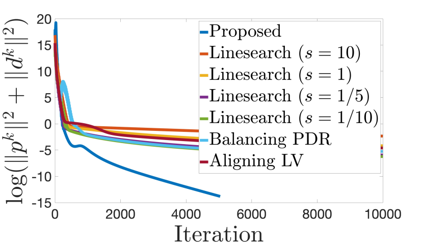
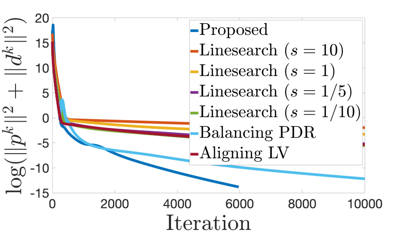
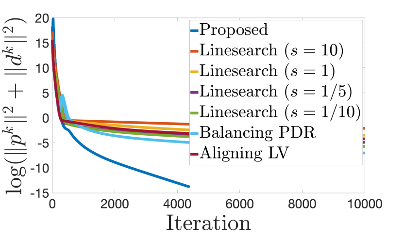
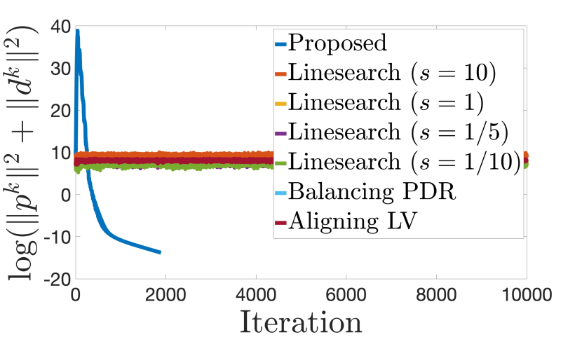
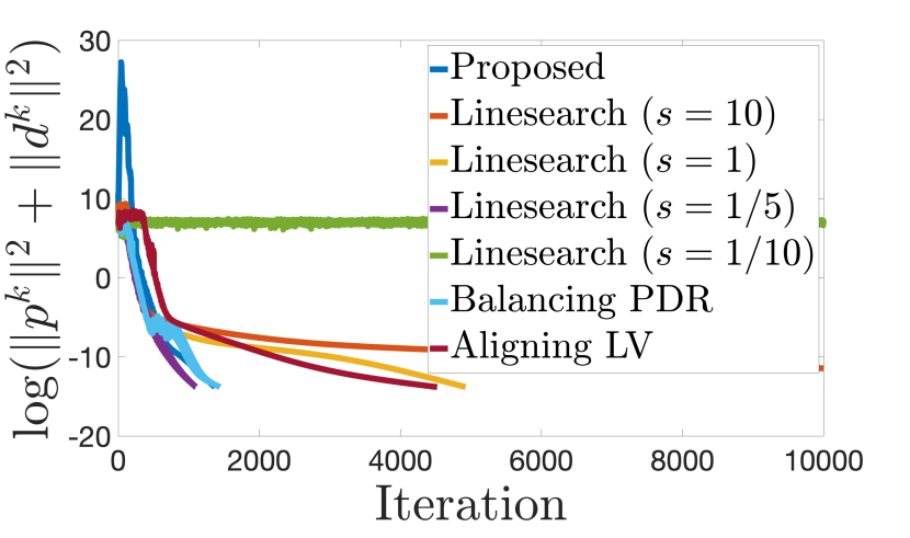
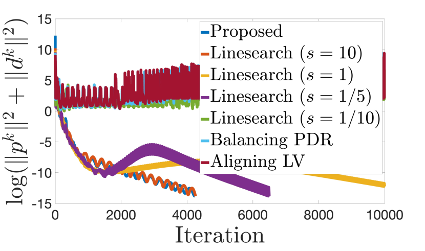
Figure 1: The rows from top to bottom are the results of RG, MC, and SNL. The columns from left to right are the results of rng(1), rng(2), rng(3), and rng(4).

RG	Proposed	LS $(s=10)$	LS $(s=1)$	LS $(s=1/5)$	LS $(s=1/10)$	B-PDR	A-LV
$<5000$	$38\%$	$5\%$	$0\%$	$1\%$	$3\%$	$8\%$	$3\%$
$<10000$	$55\%$	$21\%$	$22\%$	$17\%$	$18\%$	$34\%$	$41\%$
$<25000$	$89\%$	$78\%$	$62\%$	$75\%$	$80\%$	$73\%$	$76\%$
MC	Proposed	LS $(s=10)$	LS $(s=1)$	LS $(s=1/5)$	LS $(s=1/10)$	B-PDR	A-LV
$<2500$	$70\%$	$0\%$	$7\%$	$23\%$	$20\%$	$45\%$	$33\%$
$<5000$	$87\%$	$25\%$	$19\%$	$26\%$	$35\%$	$69\%$	$36\%$
$<10000$	$91\%$	$63\%$	$80\%$	$73\%$	$69\%$	$88\%$	$66\%$
SNL	Proposed	LS $(s=10)$	LS $(s=1)$	LS $(s=1/5)$	LS $(s=1/10)$	B-PDR	A-LV
$<7500$	$24\%$	$22\%$	$0\%$	$10\%$	$5\%$	$11\%$	$1\%$
$<15000$	$60\%$	$30\%$	$27\%$	$25\%$	$16\%$	$34\%$	$41\%$
$<30000$	$73\%$	$54\%$	$33\%$	$59\%$	$40\%$	$62\%$	$62\%$

Table 1: The blocks from top to bottom are the results of RG, MC, and SNL.

Appendix A Appendix

A.1   Proof of Theorem 2.1

See 2.1

Proof.

The core idea of the proof comes from Section 4 of [18], which shows that PDHG can be viewed as a special case of DRS. It allows us to translate known convergence results from [16] on non-stationary DRS to Algorithm 1.

We first show that Algorithm 1 is a instance of non-stationary DRS, which is extensively studied in [16],

$$z^{k+1}=J_{\alpha_{k}A}\left(J_{\alpha_{k-1}B}(z^{k})+\frac{\alpha_{k}}{\alpha_{k-1}}\Big{(}J_{\alpha_{k-1}B}(z^{k})-z^{k}\Big{)}\right)+\frac{\alpha_{k}}{\alpha_{k-1}}\left(z^{k}-J_{\alpha_{k-1}B}(z^{k})\right),$$

where $A$ and $B$ are two maximally monotone operators. Note that if the stepsize is fixed, non-stationary DRS is reduced to the vanilla one

$$z^{k+1}=J_{\alpha A}\left(2J_{\alpha B}(z^{k})-z^{k}\right)+z^{k}-J_{\alpha B}(z^{k}).$$

Similar to [18], we introduce a linear operator $\mathcal{T}\colon\mathbb{S}^{n\times n}\to\mathbb{R}^{m}$ and then reformulate the primal form of SDP (1) as

$$\min_{X}\quad\langle C,X\rangle+\mathbb{I}_{\mathbb{S}_{+}^{n\times n}}(X)+\mathbb{I}_{=0}(\hat{X})+\mathbb{I}_{=b}\left(\mathcal{A}(X)+\mathcal{T}(\hat{X})\right),$$

which is equivalent to the following monotone inclusion problem:

$$\text{Find}\ \begin{pmatrix}X\\ \hat{X}\end{pmatrix}\quad\text{s.t.}\quad 0\in\underbrace{\begin{pmatrix}C\\ 0\end{pmatrix}+\begin{pmatrix}\partial_{X}\mathbb{I}_{\mathbb{S}_{+}^{n\times n}}(X)\\ 0\end{pmatrix}+\begin{pmatrix}0\\ \partial_{\hat{X}}\mathbb{I}_{=0}(\hat{X})\end{pmatrix}}_{B=\partial f(X,\hat{X})}+\underbrace{\begin{pmatrix}\partial_{X}\mathbb{I}_{=b}(\mathcal{A}(X)+\mathcal{T}(\hat{X}))\\ \partial_{\hat{X}}\mathbb{I}_{=b}(\mathcal{A}(X)+\mathcal{T}(\hat{X}))\end{pmatrix}}_{A=\partial g(X,\hat{X})},$$ (3)

where $\partial f(X,\hat{X})$ and $\partial g(X,\hat{X})$ are maximally monotone. Applying non-stationary DRS to (3) with $z=\begin{pmatrix}X\\ \hat{X}\end{pmatrix}$, we get the following fixed-point iteration:

$$\begin{pmatrix}X^{k}\\ \hat{X}^{k}\end{pmatrix}=J_{\alpha_{k-1}\partial f}\Bigg{(}\begin{pmatrix}Z^{k}\\ \hat{Z}^{k}\end{pmatrix}\Bigg{)}$$ (4)

$$\begin{pmatrix}X^{k+\frac{1}{2}}\\ \hat{X}^{k+\frac{1}{2}}\end{pmatrix}=J_{\alpha_{k}\partial g}\Bigg{(}\begin{pmatrix}X^{k}\\ \hat{X}^{k}\end{pmatrix}+\theta_{k}\bigg{(}\begin{pmatrix}X^{k}\\ \hat{X}^{k}\end{pmatrix}-\begin{pmatrix}Z^{k}\\ \hat{Z}^{k}\end{pmatrix}\bigg{)}\Bigg{)}$$ (5)

$$\begin{pmatrix}Z^{k+1}\\ \hat{Z}^{k+1}\end{pmatrix}=\begin{pmatrix}X^{k+\frac{1}{2}}\\ \hat{X}^{k+\frac{1}{2}}\end{pmatrix}+\theta_{k}\Bigg{(}\begin{pmatrix}Z^{k}\\ \hat{Z}^{k}\end{pmatrix}-\begin{pmatrix}X^{k}\\ \hat{X}^{k}\end{pmatrix}\Bigg{)}.$$ (6)

(4) can be simplified to

$$X^{k} =\operatorname*{arg\,min}_{X}\Big{\{}\langle C,X\rangle+\mathbb{I}_{\mathbb{S}_{+}^{n\times n}}(X)+\frac{1}{2\alpha_{k-1}}\left\lVert\,X-Z^{k}\,\right\rVert^{2}\Big{\}}$$ (7)

$$\hat{X}^{k} =0$$

(5) can be simplified to

$$\begin{pmatrix}X^{k+\frac{1}{2}}\\ \hat{X}^{k+\frac{1}{2}}\end{pmatrix} =J_{\alpha_{k}\partial g}\Bigg{(}\begin{pmatrix}X^{k}\\ \hat{X}^{k}\end{pmatrix}+\theta_{k}\bigg{(}\begin{pmatrix}X^{k}\\ \hat{X}^{k}\end{pmatrix}-\begin{pmatrix}Z^{k}\\ \hat{Z}^{k}\end{pmatrix}\bigg{)}\Bigg{)}{}$$

$$=\Bigg{(}1+\alpha_{k}\partial g\Bigg{)}^{-1}\Bigg{(}\begin{pmatrix}X^{k}\\ \hat{X}^{k}\end{pmatrix}+\theta_{k}\bigg{(}\begin{pmatrix}X^{k}\\ \hat{X}^{k}\end{pmatrix}-\begin{pmatrix}Z^{k}\\ \hat{Z}^{k}\end{pmatrix}\bigg{)}\Bigg{)}{}$$

$$\Longleftrightarrow{}$$

$$\begin{pmatrix}X^{k}+\theta_{k}(X^{k}-Z^{k})\\ -\theta_{k}\hat{Z}^{k}\end{pmatrix}\in\begin{pmatrix}X^{k+\frac{1}{2}}\\ \hat{X}^{k+\frac{1}{2}}\end{pmatrix}+\alpha_{k}\mathcal{A}^{T}\bigg{(}\partial\mathbb{I}_{=b}\Big{(}\mathcal{A}\big{(}X^{k+\frac{1}{2}})+\mathcal{T}\big{(}\hat{X}^{k+\frac{1}{2}})\Big{)}\bigg{)}{}$$

$$\Longleftrightarrow{}$$

$$y^{k+1}\in\partial\mathbb{I}_{=b}\Big{(}\mathcal{A}\big{(}X^{k+\frac{1}{2}})+\mathcal{T}\big{(}\hat{X}^{k+\frac{1}{2}})\Big{)}{}$$

$$X^{k+\frac{1}{2}}+\alpha_{k}\mathcal{A}^{T}(y^{k+1})=X^{k}+\theta_{k}(X^{k}-Z^{k}){}$$

$$\hat{X}^{k+\frac{1}{2}}+\alpha_{k}\mathcal{T}^{T}(y^{k+1})=-\theta_{k}\hat{Z}^{k}{}$$

$$\Longleftrightarrow{}$$

$$\mathcal{A}\big{(}X^{k+\frac{1}{2}})+\mathcal{T}\big{(}\hat{X}^{k+\frac{1}{2}})\in\partial_{y}\mathbb{I}^{*}_{=b}(y^{k+1}){}$$

$$X^{k+\frac{1}{2}}=X^{k}+\theta_{k}(X^{k}-Z^{k})-\alpha_{k}\mathcal{A}^{T}(y^{k+1}){}$$

$$\hat{X}^{k+\frac{1}{2}}=-\theta_{k}\hat{Z}^{k}-\alpha_{k}\mathcal{T}^{T}(y^{k+1}){}$$

$$\Longleftrightarrow{}$$

$$\mathcal{A}\big{(}X^{k}+\theta_{k}(X^{k}-Z^{k})\big{)}-\theta_{k}\mathcal{T}\big{(}\hat{Z}^{k}\big{)}-\alpha_{k}\mathcal{A}\big{(}\mathcal{A}^{T}(y^{k+1})\big{)}-\alpha_{k}\mathcal{T}\big{(}\mathcal{T}^{T}(y^{k+1})\big{)}\in\partial_{y}\mathbb{I}^{*}_{=b}(y^{k+1}){}$$

$$X^{k+\frac{1}{2}}=X^{k}+\theta_{k}(X^{k}-Z^{k})-\alpha_{k}\mathcal{A}^{T}(y^{k+1}){}$$

$$\hat{X}^{k+\frac{1}{2}}=-\theta_{k}\hat{Z}^{k}-\alpha_{k}\mathcal{T}^{T}(y^{k+1}){}$$

$$\Longleftrightarrow{}$$

$$y^{k+1}=\operatorname*{arg\,min}_{y}\Big{\{}\mathbb{I}_{=b}^{*}(y)-\Big{\langle}\mathcal{A}\big{(}X^{k}+\theta_{k}(X^{k}-Z^{k})\big{)}-\theta_{k}\mathcal{T}\big{(}\hat{Z}^{k}\big{)},y\Big{\rangle}{}$$

$$\quad\quad\quad\quad\quad+\frac{\alpha_{k}}{2}(\left\lVert\,\mathcal{A}^{T}(y)\,\right\rVert^{2}+\left\lVert\,\mathcal{T}^{T}(y)\,\right\rVert^{2})\Big{\}}$$ (8)

$$X^{k+\frac{1}{2}}=X^{k}+\theta_{k}(X^{k}-Z^{k})-\alpha_{k}\mathcal{A}^{T}(y^{k+1}){}$$

$$\hat{X}^{k+\frac{1}{2}}=-\theta_{k}\hat{Z}^{k}-\alpha_{k}\mathcal{T}^{T}(y^{k+1}){},$$

(6) can be simplified to

$$Z^{k+1} =X^{k}-\alpha_{k}\mathcal{A}^{T}(y^{k+1})$$ (9)

$$\hat{Z}^{k+1} =-\alpha_{k}\mathcal{T}^{T}(y^{k+1}).$$ (10)

Substituting (9) into (7), we get

$$X^{k} =\operatorname*{arg\,min}_{X}\Big{\{}\langle C,X\rangle+\mathbb{I}_{\mathbb{S}_{+}^{n\times n}}(X)+\frac{1}{2\alpha_{k-1}}\left\lVert\,X-\big{(}X^{k-1}-\alpha_{k-1}\mathcal{A}^{T}(y^{k})\big{)}\,\right\rVert^{2}\Big{\}}$$

$$=\text{Prox}_{\alpha_{k-1}\left(\langle C,\cdot\rangle+\mathbb{I}_{\mathbb{S}_{+}^{n\times n}}(\cdot)\right)}\Big{(}X^{k-1}-\alpha_{k-1}\mathcal{A}^{T}(y^{k})\Big{)}$$

$$=\text{Prox}_{\alpha_{k-1}\mathbb{I}_{\mathbb{S}_{+}^{n\times n}}(\cdot)}\Big{(}X^{k-1}-\alpha_{k-1}\mathcal{A}^{T}(y^{k})-\alpha_{k-1}C\Big{)}$$

$$=\text{Proj}_{\mathbb{S}_{+}^{n\times n}}\Big{(}X^{k-1}-\alpha_{k-1}\mathcal{A}^{T}(y^{k})-\alpha_{k-1}C\Big{)}$$ (11)

Substituting (9) and (10) into (8), we get

$$y^{k+1} =\operatorname*{arg\,min}_{y}\Big{\{}\mathbb{I}_{=b}^{*}(y)-\langle\mathcal{A}(X^{k}+\theta_{k}(X^{k}-X^{k-1})),y\rangle+\frac{\alpha_{k}}{2}\left\lVert\,y-y^{k}\,\right\rVert^{2}_{\mathcal{A}\mathcal{A}^{T}+\mathcal{T}\mathcal{T}^{T}}\Big{\}}.$$

By Lemma A.1, we can find a $\mathcal{T}$ such that $\mathcal{T}\mathcal{T}^{T}=\frac{1}{R}\mathcal{I}-\mathcal{A}\mathcal{A}^{T}$, $\alpha_{k}\beta_{k}=R<\frac{1}{\lambda_{\max}(\mathcal{A}^{T}\mathcal{A})}$ for $k=1,2,\dots$, and then get

$$y^{k+1} =\text{Prox}_{\beta_{k}\left(\mathbb{I}_{=b}(\cdot)\right)^{*}}(y^{k}+\beta_{k}\mathcal{A}(X^{k}-\theta_{k}(X^{k}-X^{k-1})))$$

$$=y^{k}+\beta_{k}\mathcal{A}(X^{k+1}-\theta_{k}(X^{k}-X^{k-1}))-\beta_{k}\text{Prox}_{\frac{1}{\beta_{k}}\mathbb{I}_{=b}(\cdot)}(\frac{y^{k}+\beta_{k}\mathcal{A}(X^{k}-\theta_{k}(X^{k}-X^{k-1}))}{\beta_{k}})$$

$$=y^{k}+\beta_{k}\mathcal{A}(X^{k}-\theta_{k}(X^{k}-X^{k-1}))-\beta_{k}\text{Proj}_{=b}(\frac{y^{k}+\beta_{k}\mathcal{A}(X^{k}-\theta_{k}(X^{k}-X^{k-1}))}{\beta_{k}})$$

$$=y^{k}+\beta_{k}\mathcal{A}(X^{k}-\theta_{k}(X^{k}-X^{k-1}))-\beta_{k}b.$$

Finally, we have

$$X^{k}=\text{Proj}_{\mathbb{S}_{+}^{n\times n}}\Big{(}X^{k-1}-\alpha_{k-1}\mathcal{A}^{T}(y^{k})-\alpha_{k-1}C\Big{)}$$

$$y^{k+1}=y^{k}+\beta_{k}\mathcal{A}(X^{k}-\theta_{k}(X^{k}-X^{k-1}))-\beta_{k}b$$

where $X^{k}$ and $y^{k+1}$ are the primal and dual variables of SDP, respectively. Since Algorithm 1 is an instance of non-stationary DRS, we can conclude the proof by Theorem A.1. ∎

Lemma A.1.

There exists linear operator $\mathcal{T}\colon\mathbb{R}^{n\times n}\rightarrow\mathbb{R}^{m}$ such that $\mathcal{T}\mathcal{T}^{T}=\frac{1}{R}\mathcal{I}-\mathcal{A}\mathcal{A}^{T}$.

Proof.

A constructive proof is provided here. Let the vectorization of $X,A_{1},\dots,A_{m}$ be $\text{vec}(X),\text{vec}(A_{1}),\dots,\text{vec}(A_{m})\in\mathbb{R}^{n^{2}}$, respectively. Define the matrix representation of linear operators $\mathcal{T}$ and $\mathcal{A}$ as

$$T=\begin{bmatrix}\text{vec}(T_{1})^{T}\\ \vdots\\ \text{vec}(T_{m})^{T}\end{bmatrix}\in\mathbb{R}^{m\times n^{2}},\quad A=\begin{bmatrix}\text{vec}(A_{1})^{T}\\ \vdots\\ \text{vec}(A_{m})^{T}\end{bmatrix}\in\mathbb{R}^{m\times n^{2}}.$$

Define $S:=\frac{1}{R}I-AA^{T}\succ 0$. Since $m\leq n^{2}$, $T$ can be constructed as

$$T=\begin{bmatrix}\sqrt{\lambda_{1}}v_{1}\\ \vdots\\ \sqrt{\lambda_{m}}v_{m}\\ \mathbf{0}^{m\times(n^{2}-m)}\end{bmatrix},$$

where $S$ is eigenvalue-decomposed as $S=\sum_{i=1}^{m}\lambda_{i}v_{i}v_{i}^{T}$. Since $TT^{T}=S$, $T$ is the desired matrix representation of $\mathcal{T}$. Therefore, we have explicitly construct the linear operator $\mathcal{T}$. ∎

Theorem A.1.

Let $A$ and $B$ be maximally monotone and $\{\alpha_{k}\}_{k}$ be a positive sequence such as

$$\alpha_{k}\in\left(\alpha_{\min},\alpha_{\max}\right),\quad\sum_{k=1}^{\infty}\left|\alpha_{k+1}-\alpha_{k}\right|<\infty,$$

where $0<\alpha_{\min}\leq\alpha_{\max}<\infty$. Then non-stationary DRM

$$z^{k+1}=J_{\alpha_{k}A}\left(J_{\alpha_{k-1}B}(z^{k})+\frac{\alpha_{k}}{\alpha_{k-1}}\Big{(}J_{\alpha_{k-1}B}(z^{k})-z^{k}\Big{)}\right)+\frac{\alpha_{k}}{\alpha_{k-1}}\left(z^{k}-J_{\alpha_{k-1}B}(z^{k})\right),$$

weakly converges to $z^{*}$ such that $0\in(A+B)(z^{*})$.

Proof.

It is the restatement of Theorem 3.2. of [16]. ∎

A.2   Proof of Theorem 2.2

See 2.2

Proof.

Since $\theta_{k}=\frac{\alpha_{k}}{\alpha_{k-1}}$ and $\alpha_{k}\beta_{k}=R<\frac{1}{\lambda_{\max}\left(\mathcal{A}^{T}\mathcal{A}\right)}$ are automatically satisfied by Algorithm 2 and 3, it suffices to shows $\alpha_{k}\in\left(\alpha_{\min},\alpha_{\max}\right)$ and $\sum_{k=1}^{\infty}\left|\alpha_{k+1}-\alpha_{k}\right|<\infty$. To prove the boundedness of $\alpha_{k}$, we assume $\alpha_{k}$ is increased at each iteration without loss of generality, i.e., $\alpha_{k+1}=\frac{\alpha_{k}}{1-\epsilon_{k}}=\alpha_{0}\prod_{i=0}^{k+1}\frac{1}{1-\epsilon_{i}}=\alpha_{0}\prod_{i=0}^{k+1}\frac{1}{1-\epsilon_{0}\eta^{i}}$. We wish to show $\left\{\alpha_{k}\right\}$ is a convergent sequence, so that it is bounded. And it is sufficient to show $\left\{x_{k}\right\}$, where $x_{k+1}=\log\left(\prod_{i=0}^{k+1}\frac{1}{1-\epsilon_{i}}\right)=\sum_{i=0}^{k+1}\log\left(\frac{1}{1-\epsilon_{0}\eta^{i}}\right)$, is convergent since $\alpha_{0}$ is a constant. Since $\lim_{x\to 0}\frac{\ln(1+x)}{x}=1$, we have

$$\lim_{i\to\infty}\frac{\log\left(\frac{1}{1-\epsilon_{0}\eta^{i+1}}\right)}{\log\left(\frac{1}{1-\epsilon_{0}\eta^{i}}\right)}=\lim_{i\to\infty}\frac{\log\left(\frac{1}{1-\epsilon_{0}\eta^{i+1}}\right)}{\frac{\epsilon_{0}\eta^{i+1}}{1-\epsilon_{0}\eta^{i+1}}}\times\frac{\frac{\epsilon_{0}\eta^{i+1}}{1-\epsilon_{0}\eta^{i+1}}}{\frac{\epsilon_{0}\eta^{i}}{1-\epsilon_{0}\eta^{i}}}\times\frac{\frac{\epsilon_{0}\eta^{i}}{1-\epsilon_{0}\eta^{i}}}{\log\left(\frac{1}{1-\epsilon_{0}\eta^{i}}\right)}=\lim_{i\to\infty}\frac{\eta-\eta^{i+1}\epsilon_{0}}{1-\eta^{i+1}\epsilon_{0}}=\eta<1.$$

By ratio test, $x_{n}$ is convergent. We now show that $\sum_{k=1}^{\infty}\left|\alpha_{k+1}-\alpha_{k}\right|<\infty$. Since $1-\epsilon_{0}\eta^{k}>\frac{1}{2}\Leftrightarrow\log\left(\frac{1}{2\epsilon_{0}}\right)>k\log\left(\eta\right)\Leftrightarrow\underbrace{\frac{\log\left(\frac{1}{2\epsilon_{0}}\right)}{\log\left(\eta\right)}}_{=k^{*}}>k$, we have

$$\sum_{k=0}^{\infty}\left|\alpha_{k+1}-\alpha_{k}\right| \leq\sum_{k=0}^{\infty}\left|\frac{\alpha_{k}}{1-\epsilon_{k}}-\alpha_{k}\right|+\sum_{k=0}^{\infty}\left|(1-\epsilon_{k})\alpha_{k}-\alpha_{k}\right|+\sum_{k=0}^{\infty}\left|\alpha_{k}-\alpha_{k}\right|$$

$$\leq\sum_{k=0}^{\infty}\frac{\epsilon_{k}}{1-\epsilon_{k}}\alpha_{k}+\sum_{k=0}^{\infty}\epsilon_{k}\alpha_{k}$$

$$\leq\alpha_{\max}\sum_{k=0}^{\infty}\left(\frac{\epsilon_{k}}{1-\epsilon_{k}}+\epsilon_{k}\right)$$

$$=\alpha_{\max}\sum_{k=0}^{\infty}\left(\frac{\epsilon_{0}\eta^{k}}{1-\epsilon_{0}\eta^{k}}+\epsilon_{0}\eta^{k}\right)$$

$$\leq\alpha_{\max}\sum_{k=0}^{\left\lceil k^{*}\right\rceil}\left(\frac{\epsilon_{0}\eta^{k}}{1-\epsilon_{0}\eta^{k}}+\epsilon_{0}\eta^{k}\right)+\alpha_{\max}\sum_{k=\left\lceil k^{*}\right\rceil+1}^{\infty}\left(\frac{\epsilon_{0}\eta^{k}}{\frac{1}{2}}+\epsilon_{0}\eta^{k}\right)$$

$$=\alpha_{\max}\sum_{k=0}^{\left\lceil k^{*}\right\rceil}\left(\frac{\epsilon_{0}\eta^{k}}{1-\epsilon_{0}\eta^{k}}+\epsilon_{0}\eta^{k}\right)+3\epsilon_{0}\alpha_{\max}\sum_{k=\left\lceil k^{*}\right\rceil+1}^{\infty}\eta^{k}$$

$$=\alpha_{\max}\sum_{k=0}^{\left\lceil k^{*}\right\rceil}\left(\frac{\epsilon_{0}\eta^{k}}{1-\epsilon_{0}\eta^{k}}+\epsilon_{0}\eta^{k}\right)+3\epsilon_{0}\alpha_{\max}\frac{\eta^{\left\lceil k^{*}\right\rceil+1}}{1-\eta}<\infty.$$

We then conclude the proof by Theorem A.1. ∎

A.3   Proof of Theorem 2.3

See 2.3

Proof.

Since $\langle C,X\rangle+\mathbb{I}_{\mathbb{S}_{+}^{n\times n}}(X)+\mathbb{I}_{=0}(\hat{X})$ and $\mathbb{I}_{=b}(\mathcal{A}(X)+\mathcal{T}(\hat{X}))$ are closed, convex, proper functions with respect to $\begin{pmatrix}X\\ \hat{X}\end{pmatrix}$, we have

$$\begin{pmatrix}C\\ 0\end{pmatrix}+\begin{pmatrix}\partial_{X}\mathbb{I}_{\mathbb{S}_{+}^{n\times n}}(X)\\ 0\end{pmatrix}+\begin{pmatrix}0\\ \partial_{\hat{X}}\mathbb{I}_{=0}(\hat{X})\end{pmatrix}$$

and

$$\begin{pmatrix}\partial_{X}\mathbb{I}_{=b}(\mathcal{A}(X)+\mathcal{T}(\hat{X}))\\ \partial_{\hat{X}}\mathbb{I}_{=b}(\mathcal{A}(X)+\mathcal{T}(\hat{X}))\end{pmatrix}$$

are maximally monotone operators. Since

$$\omega_{i}\min\{|1-\theta_{\text{min}}|,|1-\theta_{\text{max}}|\}\leq|(1-\omega_{i}+\omega_{i}\theta_{i})-1|=\omega_{i}|1-\theta_{i}|\leq\omega_{i}\max\{|1-\theta_{\text{min}}|,|1-\theta_{\text{max}}|\},$$

$\omega_{i}>0,\ \forall i$ and $\sum_{i=0}^{\infty}\omega_{i}<\infty$, we have $\sum_{i=0}^{\infty}|(1-\omega_{i}+\omega_{i}\theta_{i})-1|<\infty$. It implies $(1-\omega_{i}+\omega_{i}\theta_{i})\rightarrow 1$ and $\prod_{i=1}^{k}(1-\omega_{i}+\omega_{i}\theta_{i})\rightarrow c$ for a certain $c\in\mathbb{R}_{++}$. Therefore, we have

$$\alpha_{k}=(1-\omega_{k}+\omega_{k}\theta_{k})\alpha_{k-1}=\prod_{i=1}^{k}(1-\omega_{i}+\omega_{i}\theta_{i})\alpha_{0}\rightarrow c\alpha_{0}>0\Longrightarrow\sum_{i=1}^{\infty}|\alpha_{k}-\alpha_{k-1}|<\infty.$$

Moreover, since

$$\theta_{\text{min}}=\min\{1,\theta_{\text{min}}\}\leq(1-\omega_{i}+\omega_{i}\theta_{\text{min}})\leq(1-\omega_{i}+\omega_{i}\theta_{i})\leq(1-\omega_{i}+\omega_{i}\theta_{\text{max}})\leq\max\{1,\theta_{\text{max}}\}=\theta_{\text{max}},$$

we have

$$\theta_{\text{min}}\alpha_{0}\leq\alpha_{k}=\prod_{i=1}^{k}(1-\omega_{i}+\omega_{i}\theta_{i})\alpha_{0}\leq\theta_{\text{max}}\alpha_{0},$$

which implies $\alpha_{k}$ is uniformly bounded. We then conclude the proof by Theorem A.1. ∎

References

• [1] Aws Albarghouthi “Introduction to neural network verification” In Foundations and Trends® in Programming Languages 7.1–2 Now Publishers, Inc., 2021, pp. 1–157
• [2] David Applegate et al. “Practical large-scale linear programming using primal-dual hybrid gradient” In Advances in Neural Information Processing Systems 34, 2021, pp. 20243–20257
• [3] Afonso S Bandeira, Nicolas Boumal and Vladislav Voroninski “On the low-rank approach for semidefinite programs arising in synchronization and community detection” In Conference on learning theory, 2016, pp. 361–382 PMLR
• [4] Stephen Boyd et al. “Distributed optimization and statistical learning via the alternating direction method of multipliers” In Foundations and Trends® in Machine learning 3.1 Now Publishers, Inc., 2011, pp. 1–122
• [5] Antonin Chambolle and Thomas Pock “A first-order primal-dual algorithm for convex problems with applications to imaging” In Journal of mathematical imaging and vision 40 Springer, 2011, pp. 120–145
• [6] Laurent Condat “A primal–dual splitting method for convex optimization involving Lipschitzian, proximable and linear composite terms” In Journal of optimization theory and applications 158.2 Springer, 2013, pp. 460–479
• [7] Alexandre d’Aspremont, Laurent Ghaoui, Michael Jordan and Gert Lanckriet “A direct formulation for sparse PCA using semidefinite programming” In Advances in neural information processing systems 17, 2004
• [8] Jim Douglas and Henry H Rachford “On the numerical solution of heat conduction problems in two and three space variables” In Transactions of the American mathematical Society 82.2, 1956, pp. 421–439
• [9] Murat A Erdogdu, Yash Deshpande and Andrea Montanari “Inference in graphical models via semidefinite programming hierarchies” In Advances in Neural Information Processing Systems 30, 2017
• [10] Michael Garstka, Mark Cannon and Paul Goulart “COSMO: A conic operator splitting method for convex conic problems” In Journal of Optimization Theory and Applications 190.3 Springer, 2021, pp. 779–810
• [11] Tom Goldstein, Min Li and Xiaoming Yuan “Adaptive primal-dual splitting methods for statistical learning and image processing” In Advances in neural information processing systems 28, 2015
• [12] Tom Goldstein et al. “Adaptive primal-dual hybrid gradient methods for saddle-point problems” In arXiv preprint arXiv:1305.0546, 2013
• [13] Gurobi Optimization, LLC “Gurobi Optimizer Reference Manual”, 2023 URL: https://www.gurobi.com
• [14] Brian Kulis, Arun C Surendran and John C Platt “Fast low-rank semidefinite programming for embedding and clustering” In Artificial Intelligence and Statistics, 2007, pp. 235–242 PMLR
• [15] Pierre-Louis Lions and Bertrand Mercier “Splitting algorithms for the sum of two nonlinear operators” In SIAM Journal on Numerical Analysis 16.6 SIAM, 1979, pp. 964–979
• [16] Dirk A Lorenz and Quoc Tran-Dinh “Non-stationary Douglas–Rachford and alternating direction method of multipliers: adaptive step-sizes and convergence” In Computational Optimization and Applications 74.1 Springer, 2019, pp. 67–92
• [17] Yura Malitsky and Thomas Pock “A first-order primal-dual algorithm with linesearch” In SIAM Journal on Optimization 28.1 SIAM, 2018, pp. 411–432
• [18] Daniel O’Connor and Lieven Vandenberghe “On the equivalence of the primal-dual hybrid gradient method and Douglas–Rachford splitting” In Mathematical Programming 179.1-2 Springer, 2020, pp. 85–108
• [19] Brendan O’donoghue, Eric Chu, Neal Parikh and Stephen Boyd “Conic optimization via operator splitting and homogeneous self-dual embedding” In Journal of Optimization Theory and Applications 169 Springer, 2016, pp. 1042–1068
• [20] Jiming Peng and Yu Wei “Approximating k-means-type clustering via semidefinite programming” In SIAM journal on optimization 18.1 SIAM, 2007, pp. 186–205
• [21] Benjamin Recht, Maryam Fazel and Pablo A Parrilo “Guaranteed minimum-rank solutions of linear matrix equations via nuclear norm minimization” In SIAM review 52.3 SIAM, 2010, pp. 471–501
• [22] Mario Souto, Joaquim D Garcia and Álvaro Veiga “Exploiting low-rank structure in semidefinite programming by approximate operator splitting” In Optimization 71.1 Taylor & Francis, 2022, pp. 117–144
• [23] Defeng Sun, Kim-Chuan Toh, Yancheng Yuan and Xin-Yuan Zhao “SDPNAL+: A Matlab software for semidefinite programming with bound constraints (version 1.0)” In Optimization Methods and Software 35.1 Taylor & Francis, 2020, pp. 87–115
• [24] Zaiwen Wen, Donald Goldfarb and Wotao Yin “Alternating direction augmented Lagrangian methods for semidefinite programming” In Mathematical Programming Computation 2.3-4 Springer, 2010, pp. 203–230
• [25] Tatsuya Yokota and Hidekata Hontani “An Efficient Method for Adapting Step-size Parameters of Primal-dual Hybrid Gradient Method in Application to Total Variation Regularization” In 2017 Asia-Pacific Signal and Information Processing Association Annual Summit and Conference (APSIPA ASC), 2017, pp. 973–979 IEEE
• [26] Lena Zdun and Christina Brandt “Fast MPI reconstruction with non-smooth priors by stochastic optimization and data-driven splitting” In Physics in Medicine & Biology 66.17 IOP Publishing, 2021, pp. 175004
• [27] Xin-Yuan Zhao, Defeng Sun and Kim-Chuan Toh “A Newton-CG augmented Lagrangian method for semidefinite programming” In SIAM Journal on Optimization 20.4 SIAM, 2010, pp. 1737–1765
• [28] Yang Zheng et al. “Chordal decomposition in operator-splitting methods for sparse semidefinite programs” In Mathematical Programming 180.1-2 Springer, 2020, pp. 489–532