Vertical Symbolic Regression via Deep Policy Gradient
Abstract
Vertical Symbolic Regression (VSR) recently has been proposed to expedite the discovery of symbolic equations with many independent variables from experimental data. VSR reduces the search spaces following the vertical discovery path by building from reduced-form equations involving a subset of independent variables to full-fledged ones. Proved successful by many symbolic regressors, deep neural networks are expected to further scale up VSR. Nevertheless, directly combining VSR with deep neural networks will result in difficulty in passing gradients and other engineering issues. We propose Vertical Symbolic Regression using Deep Policy Gradient (Vsr-Dpg) and demonstrate that Vsr-Dpg can recover ground-truth equations involving multiple input variables, significantly beyond both deep reinforcement learning-based approaches and previous VSR variants. Our Vsr-Dpg models symbolic regression as a sequential decision-making process, in which equations are built from repeated applications of grammar rules. The integrated deep model is trained to maximize a policy gradient objective. Experimental results demonstrate that our Vsr-Dpg significantly outperforms popular baselines in identifying both algebraic equations and ordinary differential equations on a series of benchmarks.
1 Introduction
Exciting progress has been made to accelerate scientific discovery using Artificial Intelligence (AI) [1, 2, 3]. Symbolic regression, as an important benchmark task in AI-driven scientific discovery, distills physics models in the form of symbolic equations from experiment data [4]. Notable progress in symbolic regression includes search-based methods [5], genetic programming [4, 6], Monte Carlo tree search [7, 8, 9], and deep reinforcement learning [10, 11].
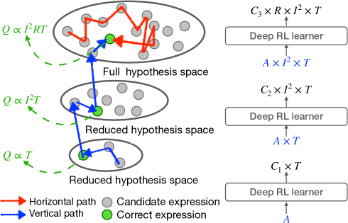
Vertical Symbolic Regression (VSR) [12, 13] recently has been proposed to expedite the discovery of symbolic equations with many independent variables. Unlike previous approaches, VSR reduces the search spaces following a vertical discovery route – it extends from reduced-form equations involving a subset of independent variables to full-fledged ones, adding one independent variable into the equation at a time. Figure 1 provides an example. To discover Joule’s law , where is heat, is current, is resistance, and is time [14], one first holds and as constants and finds . In the second round, is introduced into the equation with targeted experiments that study the effect of on . Such rounds repeat until all factors are considered. Compared with the horizontal routes, which directly model all the independent variables simultaneously, vertical discovery can be significantly cheaper because the search spaces of the first few steps are exponentially smaller than the full hypothesis space.
Meanwhile, deep learning, especially deep policy gradient [10, 11], has boosted the performance of symbolic regression approaches to a new level. Nevertheless, VSR was implemented using genetic programming. Although we hypothesize deep neural nets should boost VSR, it is not straightforward to integrate VSR with deep policy gradient-based approaches. The first idea is to employ deep neural nets to predict the symbolic equation tree in each vertical expansion step. However, this will result in (1) difficulty passing gradients from trees to deep neural nets and (2) complications concatenating deep networks for predictions in each vertical expansion step. We provide a detailed analysis of the difficulty in Appendix A.
In this work, we propose Vertical Symbolic Regression using Deep Policy Gradient (Vsr-Dpg). We demonstrate that Vsr-Dpg can recover ground-truth equations involving variables, which is beyond both deep reinforcement learning-based approaches and previous VSR variants (best up to variables). Our Vsr-Dpg solves the above difficulty based on the following key idea: each symbolic expression can be treated as repeated applications of grammar rules. Hence, discovering the best symbolic equations in the space of all candidate expressions is viewed as the sequential decision-making of predicting the optimal sequence of grammar rules.
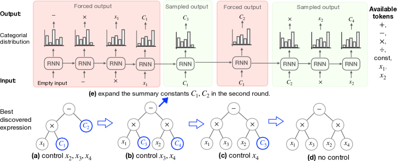
In Figure 1(right), the expansion from to is viewed as replacing constant with a sub-expression . We define a context-free grammar on symbolic expression expansion, denoting the rules that certain constants can be replaced with other variables, constants, or sub-expressions. All candidate expressions that are compatible with can be generated by repetitively applying the defined grammar rules in different order. Vsr-Dpg employs a Recurrent Neural Network (RNN) to sample many sub-expressions (including ) by sequentially sampling rules from the RNN. A vertical discovery path is built on top of this sequential decision-making process of reduced-form symbolic expressions. The RNN needs to be trained to produce expansions that lead to high fitness scores on the dataset. In this regard, we train the RNN to maximize a policy gradient objective, similar to that proposed in Petersen et al.. Our biggest difference compared with Petersen et al. is that the RNN in our Vsr-Dpg predicts the next rules in the vertical discovery space, while their model predicts the pre-order traversal of the expression tree in the full hypothesis space.
In experiments, we consider several challenging datasets of algebraic equations with multiple input variables and also of real-world differential equations in material science and biology. (1) In Table 1, our Vsr-Dpg attains the smallest median NMSE values in 7 out of 8 datasets, against a line of current popular baselines including the original VSR-GP. The main reason is deep networks offer many more parameters than the GP algorithm, which can better adapt to different datasets and sample higher-quality expressions from the deep networks. (2) Further analysis on the best-discovered equation (in Table 3) shows that Vsr-Dpg uncovers up to 50% of the exact governing equations with input variables, where the baselines only attain 0%. (3) In table 2, our Vsr-Dpg is able to find high-quality expressions on expressions with more than 50 variables, which is never the case in all the baselines. The major reason is the use of the control variable experiment. (4) On discovery of ordinary differential equations in Table 4, our Vsr-Dpg also improves over current baselines.
2 Preliminaries
Symbolic Regression aims to discover governing equations from the experimental data. An example of such mathematical expression is Joule’s first law: , which quantifies the amount of heat generated when electric current flows through a conductor with resistance for time . Formally, a mathematical expression connects a set of input variables and a set of constants by mathematical operators. The possible mathematical operators include addition, subtraction, multiplication, division, trigonometric functions, etc. The meaning of these mathematical expressions follows their standard arithmetic definition.
Given a dataset with samples, symbolic regression searches for the optimal expression , such that . From an optimization perspective, minimizes the averaged loss on the dataset:
| (1) |
Here, hypothesis space is the set of all candidate mathematical expressions; denotes the constant coefficients in the expression; denotes a loss function that penalizes the difference between the output of the candidate expression and the ground truth . The set of all possible expressions i.e., the hypothesis space , can be exponentially large. As a result, finding the optimal expression is challenging and is shown to be NP-hard [15].
Deep Policy Gradient for Symbolic Regression. Recently, a line of work proposes the use of deep reinforcement learning (RL) for searching the governing equations [10, 16, 11]. They represent expressions as binary trees, where the interior nodes correspond to mathematical operators and leaf nodes correspond to variables or constants. The key idea is to model the search of different expressions, as a sequential decision-making process for the preorder traversal sequence of the expression trees using an RL algorithm. A reward function is defined to measure how well a predicted expression can fit the dataset. The deep recurrent neural network (RNN) is used as the RL learner for predicting the next possible node in the expression tree at every step of decision-making. The parameters of the RNN are trained using a policy gradient objective.
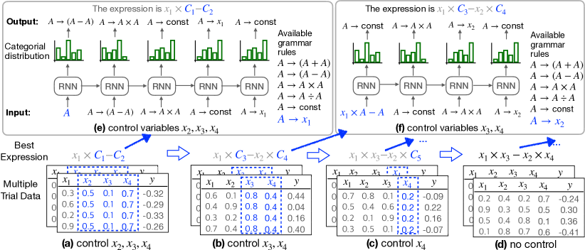
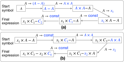
Control Variable Experiment studies the relationship between a few input variables and the output in the regression problem, with the remaining input variables fixed to be the same [17]. In the controlled setting, the ground-truth equation behaves the same after setting those controlled variables as constants, which is noted as the reduced-form equation. For example, the ground-truth equation in Figure 2(a) is reduced to when controlling . Figure 2(b,c) presents other reduced-form equations when the control variables are changed. For the corresponding dataset , the controlled variables are fixed to one value and the remaining variables are randomly assigned. See Figure 2(a,b,c) for example datasets generated under different controlling variables.
Vertical Symbolic Regression starts by finding a symbolic equation involving a small subset of the input variables and iteratively expands the discovered expression by introducing more variables. VSR relies on the control variable experiments introduced above.
VSR-GP was the first implementation of vertical symbolic regression using genetic programming (GP) [12, 13]. To fit an expression of variables, VSR-GP initially only allows variable to vary and controls the values of all the rest variables. Using GP as a subroutine, VSR-GP finds a pool of expressions which best fit the data from this controlled experiment. Notice are restricted to contain only one free variable and is the pool size. A small error indicates is close to the ground truth reduced to the one free variable and thus is marked unmutable by the genetic operations in the following rounds. In the 2nd round, VSR-GP adds a second free variable and starts fitting using the data from control variable experiments involving the two free variables . After rounds, the expressions in the VSR-GP pool consider all variables. Overall, VSR expedites the discovery process because the first few rounds of VSR are significantly cheaper than the traditional horizontal discovery process, which searches for optimal expression involving all input variables at once.
3 Methodology
Motivation. The prior work of VSR-GP uses genetic programming to edit the expression tree. GP is not allowed to edit internal nodes in the best-discovered expression trees from the previous vertical discovery step, to ensure later genetic operations do not delete the prior knowledge on the governing equation. But, this idea cannot be easily integrated with deep reinforcement learning-based symbolic regressors.
Employing deep neural nets in vertical symbolic regression to predict the symbolic equation tree in each vertical expansion step will result in (1) difficulty passing gradients from trees to deep neural nets. (2) complications in concatenating deep networks for predictions in each vertical expansion step. See two possible integrations in appendix A.
Our idea is to consider a new representation of expression. We extend the context-free grammar definition for symbolic expression, where a sequence of grammar rules uniquely corresponds to an expression. We regard the prediction of symbolic expression as the sequential decision-making process of picking the sequence of grammar rules step-by-step. The RNN predicts grammar rules instead of nodes in the expression tree. The best-discovered reduced-form equation is converted into the start symbol in the grammar, ensuring the predicted expression from our RNN is always compatible with the prior knowledge of the governing equation. This allows us to shrink the hypothesis space and accelerate scientific discovery because other non-reducible expressions will be never sampled from the RNN.
Deep Vertical Symbolic Regression Pipeline. Figure 1 shows our deep vertical symbolic regression (Vsr-Dpg) pipeline. The high-level idea of Vsr-Dpg is to construct increasingly complex symbolic expressions involving an increasing number of independent variables based on control variable experiments with fewer and fewer controlled variables.
To fit an expression of variables, we first hold all variables as constant and allow only one variable to vary. We would like to find the best expression , which best fits the data in this controlled experiment. We use the deep RNN as the RL learner to search for the best possible expression. It is achieved by using the RNN to sample sequences of grammar rules defined for symbolic expression. Every sequence of rules is then converted into an expression, where the constants in the expression are fitted with the dataset. The parameters of the RNN model will be trained through the policy gradient objective. The expression with the best fitness score is returned as the prediction of the RNN. A visualized process is in Figure 1(a, e).
Following the idea in VSR, the next step is to decide whether each constant is a summary constant or a standalone constant. (1) A constant that is not relevant to any controlled variables is considered as standalone, which will be preserved in the rest rounds. (2) A constant that is actually a sub-expression involving those controlled variables is noted as the summary type, which will be expanded in the following rounds. In our implementation, if the variance of fitted values of constant across multiple control variable experiments is high, then it is classified as the summary type. Otherwise, it is classified as a standalone type.
Assuming we find the correct reduced-from equation after several learning epochs. To ensure Vsr-Dpg does not forget this discovered knowledge of the first round, we want all the expressions to be discovered in the following rounds can be reduced to . Therefore, we construct as the start symbol for the following round by replacing every summary constant in as a non-terminal symbol in the grammar (noted as ), indicating a sub-expression. For the example case in Figure 2(a), both of them are summary constants so the 1st round best-predicted expression is converted as the 2nd round start symbol .
In the 2nd round, Vsr-Dpg adds one more free variable and starts fitting using the data from control variable experiments involving two free variables. Similar to the first round, we are restricted to only searching for sub-expressions with the second variable. It is achieved by limiting the output vocabulary of the RNN model. In Figure 2(f), the RNN model finds an expression . The semantic is that the RL learner learns to expand with another constant and with sub-expression , based on the best-discovered result of the 1st round .
Our Vsr-Dpg introduces one free variable at a time and expands the equation learned in the previous round to include this newly added variable. This process continues until all the variables are considered. After rounds, we return the equations with the best fitness scores. The predicted equation will be evaluated on data with no variable controlled. See the steps in Figure 1(b,c,d) for a visual demonstration. We summarize the whole process of Vsr-Dpg in Algorithm 1 in the appendix. The major difference of this approach from most state-of-the-art approaches is that those baselines learn to find the expressions in the full hypothesis space with all input variables, from a fixed dataset collected before training. Our Vsr-Dpg accelerates the discovery process, because of the small size of the reduced hypothesis space, i.e., the set of candidate expressions involving only a few variables. The task is much easier than fitting the expression in the full hypothesis space involving all input variables.
3.1 Expression Represented with Grammar Rules
We propose to represent symbolic expression by extending the context-free grammar (CFG) [7]. A context-free grammar is represented by a tuple , where is a set of non-terminal symbols, is a set of terminal symbols, is a set of production rules and is a start symbol. In our formulation, (1) is the set of input variables and constants . (2) set of non-terminal symbols represents sub-expressions, like . Here is a placeholder symbol. (3) set of production rules represents mathematical operations such as addition, subtraction, multiplication, and division. That is , where represents the left-hand side is replaced with its right-hand side. (4) The start symbol is extended to be , , or other symbols constructed from the best-predicted expression under the controlled variables.
Beginning with the start symbol, successive applying the grammar rules in different orders results in different expressions. Each rule expands the first non-terminal symbol in the start symbol. An expression with only terminal symbols is a valid mathematical expression, whereas an expression with a mixture of non-terminal and terminal symbols is an invalid expression. The expression can also be represented as a binary tree. We chose grammar representation instead of the binary tree for expressions because it will make the vertical symbolic regression process straightforward.
Figure 3 presents two examples of constructing the expression from the start symbol using the given sequence of grammar rules. In Figure 3(a), we first use the grammar rule for subtraction , which means that the symbol in expression is expanded with its right-hand side, resulting in . By repeatedly using grammar rules to expand the non-terminal symbols, we finally arrive at our desired expression . In Figure 3(b), the start symbol is . The rule replaces the first non-terminal symbol with a constant. Thus, we have . In the end, we obtain a valid expression .
Afterward, we decide the optimal value of open constants in each expression. Assume the expression has open constants. We first sample a batch of data with the controlled variable and then use a gradient-based optimizer to fit those open constants, by minimizing the objective . We then obtain the fitness score , the fitted constants , and the fitted equation .
3.2 Expression Sampling from Recurrent Network
Vocabulary. In our vertical symbolic regression setting, the input and output vocabulary is the set of grammar rules that cover each input variable, constants, and mathematical operations. We create an embedding layer for the input vocabulary, noted as the function. For each input rule , its -dimensional embedding vector is noted as .
Sampling Procedure. The RNN module samples an expression by sampling the sequence of grammar rules in a sequential decision-making process. Denote the sampled sequence of rules as . Initially, the RNN takes in the start symbol and computes the first step hidden state vector . At -th time step, RNN uses the predicted output from the previous step as the input of current step . RNN computes its hidden state vector using the embedding vector of input token and the previous time-step hidden state vector . The linear layer and softmax function are applied to emit a categorical distribution over every token in the output vocabulary, which represents the probability of the next possible rule in the half-completed expression . The RNN samples one token from the categorical distribution as the prediction of the next possible rule. To conclude, the computational pipeline at the -th step is shown below:
| (2) | ||||
The weight matrix and bias vector are the parameters of the linear layer and the last row in Eq. 2 is the softmax layer. are the parameters of the RNN. The sampled rule will be the input for the -th step.
After steps, we obtain the sequence of rules with probability . We convert this sequence into an expression by following the procedure described in Section 3.1. For cases where we arrive at the end of the sequence while there are still non-terminal symbols in the converted expression, we would randomly add some rules with only terminal symbols to complete the expression. For cases where we already get a valid expression in the middle of the sequence, we ignore the rest of the sequence and return the valid expression.
Policy Gradient-based Training. We follow the reinforcement learning formulation to train the parameters of the RNN module [18]. The sampled rules before the current step , i.e., (, is viewed as the state of the -th step for the RL learner. Those rules in the output vocabulary are the available actions for the RL learner. In the formulated decision-making process, the RNN takes in the current state and outputs a distribution over next-step possible actions. The objective of the RL learner is to learn to pick the optimal sequences of grammar rules to maximize the expected rewards. Denote the converted expression from as . A typical reward function is defined from the fitness score of the expression . The objective that maximizes the expected reward from the RNN model is defined as , where is the probability of sampling sequence from the RNN.
The gradient with respect to the objective needs to be estimated. We follow the classic REINFORCE policy gradient algorithm [19]. We first sample several times from the RNN module and obtain sequences , an unbiased estimation of the gradient of the objective is computed as . The parameters of the deep network are updated by the gradient descent algorithm with the estimated policy gradient value. In the literature, several practical tricks are proposed to reduce the estimation variance of the policy gradient. A common choice is to subtract a baseline function from the reward, as long as the baseline is not a function of the sample batch of expressions. Our implementation adopts this trick and the detailed derivation is presented in Appendix B. There are many variants like risk-seeking policy gradient [10], priority queue training [16].
Throughout the whole training process, the expression with optimal fitness score from all the sampled expressions is used as the prediction of Vsr-Dpg at the current round.
3.3 Construct Start Symbol from the best-predicted Expression
Given the best-predicted expression and controlled variables , the following step is to construct the start symbol of the next rounds. This operation ensures all the future expressions can be reduced to any previously discovered equation thus all the discovered knowledge is remembered. It expedites the discovery of symbolic expression since other expressions that cannot be reduced to will be never sampled from the RNN. It requires first classifying the type of every constant in the expression into stand-alone or summary type, through multi-trail control variable experiments. Then we replace each summary constant with a placeholder symbol (i.e., “”) indicating a sub-expression containing controlled variables.
Following the procedure proposed in [12], we first query data batches with the same controlled variables . The controlled variables take the same value within each batch while taking different values across data batches. We fit open constants in the candidate expression with each data batch by the gradient-based optimizer, like BFGS [20]. We obtain multiple fitness scores and multiple solutions to open constants . By examining the outcomes of -trials control variable experiments, we have: (1) Consistent close-to-zero fitness scores imply the fitted expression is close to the ground-truth equation in the reduced form. That is for all , where is the threshold for the fitness scores. (2) Conditioning on the result in case (1), the -th open constant is a standalone constant when the empirical variance of its fitted values across trials is less than a threshold . In practice, if the best-predicted expression by the RNN module is not consistently close to zero, then all the constants in the expression are summary constants. Finally, the start symbol is obtained by replacing every summary constant with the symbol “” according to our grammar.
| Methods | ||||||||
|---|---|---|---|---|---|---|---|---|
| VSR-GP | T.O. | |||||||
| GP | 0.872 | |||||||
| Eureqa | 1E-6 | 1E-6 | ||||||
| SPL | ||||||||
| E2ETransformer | 0.018 | 0.0015 | 0.030 | 0.121 | 0.142 | 0.112 | ||
| DSR | ||||||||
| PQT | ||||||||
| VPG | ||||||||
| GPMeld | T.O. | |||||||
| Vsr-Dpg (ours) | 0.114 |
4 Related Work
Recently AI has been highlighted to enable scientific discoveries in diverse domains [21, 22, 3]. Early work in this domain focuses on learning logic (symbolic) representations [23]. Recently, there has been extensive research on learning algebraic equations [10, 11] and differential learning differential equations from data [24, 25, 26, 27, 28, 29, 30, 31, 32, 33, 34]. In this domain, a line of works develops robots that automatically refine the hypothesis space, some with human interactions [1, 35, 36, 37]. These works are quite related to ours because they also actively probe the hypothesis spaces, albeit they are in biology and chemistry.
Existing works on multi-variable regression are mainly based on pre-trained encoder-decoder methods with massive training datasets (e.g., millions of data points [38]), and even larger-scale generative models (e.g., approximately 100 million parameters [39]). Our Vsr-Dpg algorithm is a tailored algorithm to solve multi-variable symbolic regression problems.
The idea of using a control variable experiment tightly connects to the BACON system [40, 41, 42, 36, 37, 43]. Our method develops on the current popular deep recurrent neural network while their method is a rule-based system, due to the historical limitation.
Our method connects to the symbolic regression method using probabilistic context-free grammar [7, 44, 45]. They use a fixed probability to sample rules, we use a deep neural network to learn the probability distribution.
Our Vsr-Dpg is also tightly connected to deep symbolic regression [10, 11]. We both use deep recurrent networks to predict a sequence of tokens that can be composed into a symbolic expression. However, their method predicts the preorder traversal sequence for the expression tree while our method predicts the sequence of production rules for the expression.
5 Experiment
In this section, we evaluate the performance of the proposed Vsr-Dpg method on several multi-variable algebraic equations datasets and further extend to real-world differential equation discovery tasks.
5.1 Symbolic Regression on Algebraic Equations
Experiment Settings. For the dataset on algebraic expressions, we consider the 8 groups of expressions from the Trigonometric dataset [12], where each group contains 10 randomly sampled expressions. In terms of baselines, we consider (1) evolutionary algorithm: Genetic Programming (GP), Control Variable Genetic Programming (CVGP) [12], and Eureqa [46]. (2) deep reinforcement learning: Priority queue training (PQT) [16], Vanilla Policy Gradient (VPG) [19], Deep Symbolic Regression (DSR) [10], and Neural-Guided Genetic Programming Population Seeding (GPMeld) [11]. (3) Monte Carlo Tree Search: Symbolic Physics Learner (SPL) [8], (4) Transformer network with pre-training: end-to-end Transformer (E2ETransformer) [39]. In terms of evaluation metrics, we evaluate the normalized-mean-squared-error (NMSE) of the best-predicted expression by each algorithm, on a separately-generated testing dataset . We report median values instead of means due to outliers. Symbolic regression belongs to combinatorial optimization problems, which commonly have no mean values. The detailed experiment configurations are in Appendix C.2.
Goodness-of-fit Comparison. We consider our Vsr-Dpg against several challenging datasets involving multiple variables. In table 1, We report the median NMSE on the selected algebraic datasets. Our Vsr-Dpg attains the smallest median NMSE values in 7 out of 8 datasets, against a line of current popular baselines including the original VSR-GP. The main reason is deep networks offer many more parameters than the GP algorithm, which can better adapt to different datasets and sample higher-quality expressions from the deep networks.
Extended Large-scale Comparison. In the real world, scientists may collect all available variables that are more than needed into symbolic regression, where only part of the inputs will be included in the ground-truth expression. We randomly pick variables from all the variables and replace the appeared variable in expressions confined as in Table 1. In Table 2, we collect the median NMSE values on this large-scale dataset setting. Our Vsr-Dpg scales well because it first detects all the contributing inputs using the control variable experiments. Notice that those baselines that are easily timeout in this setting are excluded for comparison.
| Total Input Variables | |||||
| SPL | 0.386 | 0.554 | 0.554 | 0.714 | 0.815 |
| GP | 0.159 | 0.172 | 0.218 | 0.229 | 0.517 |
| DSR | 0.284 | 0.521 | 0.522 | 0.660 | 0.719 |
| VPG | 0.415 | 0.695 | 0.726 | 0.726 | 0.779 |
| PQT | 0.384 | 0.488 | 0.615 | 0.620 | 0.594 |
| Vsr-Dpg | 0.002 | 0.021 | |||
Exact Recovery Comparison. We compare if each learning algorithm finds the exact equation, the result of which is collected in Table 3. The discovered equation by each algorithm is further collected in Appendix D.1. We can observe that our Vsr-Dpg has a higher rate of recovering the ground-truth expressions compared to baselines. This is because our method first use a control variable experiment to pick what are the contributing variables to the data and what are not.
| SPL | ||||
|---|---|---|---|---|
| E2ETransformer | ||||
| VSR-GP | ||||
| VSR-DPG | 70% | 60% |
5.2 Symbolic Regression on Differential Equations
Task Definition. The temporal evolution of the dynamic system is modeled by the time derivatives of the state variables. Let be the -dimensional vector of state variables, and is the vector of their time derivatives. The differential equation is of the form , where constant vector are parameters of the dynamic system. Following the definition of symbolic regression on differential equation in [45, 8], given a trajectory dataset of state variable and its time derivatives , the symbolic regression task is to predict the best expression that minimizes the average loss on trajectory data: . Other formulation of this problem assume we have no access to its time derivatives, that is [47].
Experiment Setting. We consider recent popular baselines for differential equations, including (1) SINDy [25], (2) ODEFormer [47], (3) Symbolic Physics Learner (SPL) [8]. 4) Probabilistic grammar for equation discovery (ProGED) [44]. In terms of the dataset, we consider the Lorenz Attractor with variables, Magnetohydrodynamic (MHD) turbulence with variables, and Glycolysis Oscillation with variables. All of them are collected from [25]. To evaluate whether the algorithm identifies the ground-truth expression, we use the Accuracy metric based on the coefficient of determination (). The detailed experiment configurations are in Appendix C.3.
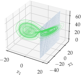
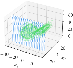
Result Analysis. The results are summarized in Table 4. Our proposed Vsr-Dpg discovers a set of differential expressions with much higher quality than the considered baselines. We further provide a visual understanding of the proposed Vsr-Dpg method in Figure 4. The data of our Vsr-Dpg are drawn from the intersection of the mesh plane and the curve on the Lorenz attractor. In comparison, the current baselines draw data by picking a random trajectory or many random points on the curve. We notice the ODEFormer is pre-trained on differential equations up to two variables, thus does not scale well with more variable settings. The predicted differential equations by each algorithm are in appendix D.2.
| Lorenz | MHD | Glycolysis | |
| SPL | 50% | ||
| SINDy | 0% | ||
| ProGED | 0% | ||
| ODEFormer | 0% | 0% | NA |
| Vsr-Dpg (ours) |
6 Conclusion
In this research, we propose Vertical Symbolic Regression with Deep Policy Gradient (i.e., Vsr-Dpg) to discover governing equations involving many independent variables, which is beyond the capabilities of current state-of-the-art approaches. Vsr-Dpg follows a vertical discovery path – it builds equations involving more and more input variables using control variable experiments. Because the first few steps following the vertical discovery route are much cheaper than discovering the equation in the full hypothesis space, Vsr-Dpg has the potential to supercharge current popular approaches. Experimental results show Vsr-Dpg can uncover complex scientific equations with more contributing factors than what current approaches can handle.
Acknowledgments
This research was supported by NSF grant CCF-1918327 and DOE – Fusion Energy Science grant: DE-SC0024583.
References
- Langley et al. [1987] Patrick W. Langley, Herbert A. Simon, Gary Bradshaw, and Jan M. Zytkow. Scientific Discovery: Computational Explorations of the Creative Process. The MIT Press, 02 1987.
- Kulkarni and Simon [1988] Deepak Kulkarni and Herbert A Simon. The processes of scientific discovery: The strategy of experimentation. Cogn. Sci., 12(2):139–175, 1988.
- Wang et al. [2023] Hanchen Wang, Tianfan Fu, Yuanqi Du, Wenhao Gao, Kexin Huang, Ziming Liu, Payal Chandak, Shengchao Liu, Peter Van Katwyk, Andreea Deac, et al. Scientific discovery in the age of artificial intelligence. Nature, 620(7972):47–60, 2023.
- Schmidt and Lipson [2009] Michael Schmidt and Hod Lipson. Distilling free-form natural laws from experimental data. Science, 324(5923):81–85, 2009.
- Lenat [1977] Douglas B. Lenat. The ubiquity of discovery. Artif. Intell., 9(3):257–285, 1977.
- Virgolin et al. [2019] Marco Virgolin, Tanja Alderliesten, and Peter A. N. Bosman. Linear scaling with and within semantic backpropagation-based genetic programming for symbolic regression. In GECCO, pages 1084–1092, 2019.
- Todorovski and Dzeroski [1997] Ljupco Todorovski and Saso Dzeroski. Declarative bias in equation discovery. In ICML, pages 376–384. Morgan Kaufmann, 1997.
- Sun et al. [2023] Fangzheng Sun, Yang Liu, Jian-Xun Wang, and Hao Sun. Symbolic physics learner: Discovering governing equations via monte carlo tree search. In ICLR, 2023.
- Kamienny et al. [2023] Pierre-Alexandre Kamienny, Guillaume Lample, Sylvain Lamprier, and Marco Virgolin. Deep generative symbolic regression with monte-carlo-tree-search. In ICML, volume 202. PMLR, 2023.
- Petersen et al. [2021] Brenden K. Petersen, Mikel Landajuela, T. Nathan Mundhenk, Cláudio Prata Santiago, Sookyung Kim, and Joanne Taery Kim. Deep symbolic regression: Recovering mathematical expressions from data via risk-seeking policy gradients. In ICLR, 2021.
- Mundhenk et al. [2021] T. Nathan Mundhenk, Mikel Landajuela, Ruben Glatt, Cláudio P. Santiago, Daniel M. Faissol, and Brenden K. Petersen. Symbolic regression via deep reinforcement learning enhanced genetic programming seeding. In NeurIPS, pages 24912–24923, 2021.
- Jiang and Xue [2023] Nan Jiang and Yexiang Xue. Symbolic regression via control variable genetic programming. In ECML/PKDD, volume 14172 of Lecture Notes in Computer Science, pages 178–195. Springer, 2023.
- Jiang et al. [2023] Nan Jiang, Md Nasim, and Yexiang Xue. Vertical symbolic regression. arXiv preprint arXiv:2312.11955, 2023.
- Joule [1843] James Prescott Joule. On the production of heat by voltaic electricity. In Abstracts of the Papers Printed in the Philosophical Transactions of the Royal Society of London, pages 280–282, 1843.
- Virgolin and Pissis [2022] Marco Virgolin and Solon P Pissis. Symbolic regression is NP-hard. TMLR, 2022.
- Abolafia et al. [2018] Daniel A. Abolafia, Mohammad Norouzi, and Quoc V. Le. Neural program synthesis with priority queue training. CoRR, abs/1801.03526, 2018.
- Lehman et al. [2004] Jeffrey S Lehman, Thomas J Santner, and William I Notz. Designing computer experiments to determine robust control variables. Statistica Sinica, pages 571–590, 2004.
- Wierstra et al. [2010] Daan Wierstra, Alexander Förster, Jan Peters, and Jürgen Schmidhuber. Recurrent policy gradients. Log. J. IGPL, 18(5):620–634, 2010.
- Williams [1992] Ronald J. Williams. Simple statistical gradient-following algorithms for connectionist reinforcement learning. Mach. Learn., 8:229–256, 1992.
- Fletcher [2000] Roger Fletcher. Practical methods of optimization. John Wiley & Sons, 2000.
- Kirkpatrick et al. [2021] James Kirkpatrick, Brendan McMorrow, David H. P. Turban, Alexander L. Gaunt, James S. Spencer, Alexander G. D. G. Matthews, Annette Obika, Louis Thiry, Meire Fortunato, David Pfau, Lara Román Castellanos, Stig Petersen, Alexander W. R. Nelson, Pushmeet Kohli, Paula Mori-Sánchez, Demis Hassabis, and Aron J. Cohen. Pushing the frontiers of density functionals by solving the fractional electron problem. Science, 374(6573):1385–1389, 2021.
- Jumper et al. [2021] John Jumper, Richard Evans, Alexander Pritzel, Tim Green, Michael Figurnov, Olaf Ronneberger, Kathryn Tunyasuvunakool, Russ Bates, Augustin Žídek, Anna Potapenko, et al. Highly accurate protein structure prediction with alphafold. Nature, 596(7873):583–589, 2021.
- Bradley et al. [2001] Elizabeth Bradley, Matthew Easley, and Reinhard Stolle. Reasoning about nonlinear system identification. Artif. Intell., 133(1):139–188, 2001.
- Dzeroski and Todorovski [1995] Saso Dzeroski and Ljupco Todorovski. Discovering dynamics: From inductive logic programming to machine discovery. J. Intell. Inf. Syst., 4(1):89–108, 1995.
- Brunton et al. [2016] Steven L. Brunton, Joshua L. Proctor, and J. Nathan Kutz. Discovering governing equations from data by sparse identification of nonlinear dynamical systems. PNAS, 113(15):3932–3937, 2016.
- Wu and Tegmark [2019] Tailin Wu and Max Tegmark. Toward an artificial intelligence physicist for unsupervised learning. Phys. Rev. E, 100:033311, Sep 2019.
- Zhang and Lin [2018] Sheng Zhang and Guang Lin. Robust data-driven discovery of governing physical laws with error bars. Proc Math Phys Eng Sci., 474(2217), 2018.
- Iten et al. [2020] Raban Iten, Tony Metger, Henrik Wilming, Lídia Del Rio, and Renato Renner. Discovering physical concepts with neural networks. Physical review letters, 124(1):010508, 2020.
- Cranmer et al. [2020] Miles D. Cranmer, Alvaro Sanchez-Gonzalez, Peter W. Battaglia, Rui Xu, Kyle Cranmer, David N. Spergel, and Shirley Ho. Discovering symbolic models from deep learning with inductive biases. In NeurIPS, 2020.
- Raissi et al. [2020] Maziar Raissi, Alireza Yazdani, and George Em Karniadakis. Hidden fluid mechanics: Learning velocity and pressure fields from flow visualizations. Science, 367(6481):1026–1030, 2020.
- Raissi et al. [2019] M. Raissi, P. Perdikaris, and G.E. Karniadakis. Physics-informed neural networks: A deep learning framework for solving forward and inverse problems involving nonlinear partial differential equations. Journal of Computational Physics, 378:686–707, 2019.
- Liu and Tegmark [2021] Ziming Liu and Max Tegmark. Machine learning conservation laws from trajectories. Phys. Rev. Lett., 126:180604, May 2021.
- Xue et al. [2021] Yexiang Xue, Md. Nasim, Maosen Zhang, Cuncai Fan, Xinghang Zhang, and Anter El-Azab. Physics knowledge discovery via neural differential equation embedding. In ECML/PKDD, pages 118–134, 2021.
- Chen et al. [2018] Ricky TQ Chen, Yulia Rubanova, Jesse Bettencourt, and David K Duvenaud. Neural ordinary differential equations. NeurIPS, 31, 2018.
- Valdés-Pérez [1994] R.E. Valdés-Pérez. Human/computer interactive elucidation of reaction mechanisms: application to catalyzed hydrogenolysis of ethane. Catalysis Letters, 28:79–87, 1994.
- King et al. [2004] Ross D King, Kenneth E Whelan, Ffion M Jones, Philip GK Reiser, Christopher H Bryant, Stephen H Muggleton, Douglas B Kell, and Stephen G Oliver. Functional genomic hypothesis generation and experimentation by a robot scientist. Nature, 427(6971):247–252, 2004.
- King et al. [2009] Ross D. King, Jem Rowland, Stephen G. Oliver, Michael Young, Wayne Aubrey, Emma Byrne, Maria Liakata, Magdalena Markham, Pinar Pir, Larisa N. Soldatova, Andrew Sparkes, Kenneth E. Whelan, and Amanda Clare. The automation of science. Science, 324(5923):85–89, 2009.
- Biggio et al. [2021] Luca Biggio, Tommaso Bendinelli, Alexander Neitz, Aurélien Lucchi, and Giambattista Parascandolo. Neural symbolic regression that scales. In ICML, volume 139, pages 936–945. PMLR, 2021.
- Kamienny et al. [2022] Pierre-Alexandre Kamienny, Stéphane d’Ascoli, Guillaume Lample, and François Charton. End-to-end symbolic regression with transformers. In NeurIPS, 2022.
- Langley [1977] Pat Langley. BACON: A production system that discovers empirical laws. In IJCAI, page 344, 1977.
- Langley [1979] Pat Langley. Rediscovering physics with BACON.3. In IJCAI, pages 505–507, 1979.
- Langley et al. [1981] Pat Langley, Gary L. Bradshaw, and Herbert A. Simon. BACON.5: the discovery of conservation laws. In IJCAI, pages 121–126, 1981.
- Cerrato et al. [2023] Mattia Cerrato, Jannis Brugger, Nicolas Schmitt, and Stefan Kramer. Reinforcement learning for automated scientific discovery. In AAAI Spring Symposium, 2023.
- Brence et al. [2021] Jure Brence, Ljupco Todorovski, and Saso Dzeroski. Probabilistic grammars for equation discovery. Knowl. Based Syst., 224:107077, 2021.
- Gec et al. [2022] Bostjan Gec, Nina Omejc, Jure Brence, Saso Dzeroski, and Ljupco Todorovski. Discovery of differential equations using probabilistic grammars. In DS, volume 13601, pages 22–31. Springer, 2022.
- Dubcáková [2011] Renáta Dubcáková. Eureqa: software review. Genet. Program. Evolvable Mach., 12(2):173–178, 2011.
- d’Ascoli et al. [2024] Stéphane d’Ascoli, Sören Becker, Alexander Mathis, Philippe Schwaller, and Niki Kilbertus. Odeformer: Symbolic regression of dynamical systems with transformers. In ICLR. OpenReview.net, 2024.
- Koza [1994] John R Koza. Genetic programming as a means for programming computers by natural selection. Statistics and computing, 4:87–112, 1994.
- Ryan and Morgan [2007] Thomas P. Ryan and J. P. Morgan. Modern experimental design. Journal of Statistical Theory and Practice, 1(3-4):501–506, 2007.
- Chen and Xue [2022] Qi Chen and Bing Xue. Generalisation in genetic programming for symbolic regression: Challenges and future directions. In Women in Computational Intelligence: Key Advances and Perspectives on Emerging Topics, pages 281–302. Springer, 2022.
- Keren et al. [2023] Liron Simon Keren, Alex Liberzon, and Teddy Lazebnik. A computational framework for physics-informed symbolic regression with straightforward integration of domain knowledge. Scientific Reports, 13(1):1249, 2023.
- Haut et al. [2022] Nathan Haut, Wolfgang Banzhaf, and Bill Punch. Active learning improves performance on symbolic regression tasks in stackgp. In GECCO Companion, pages 550–553, 2022.
- Haut et al. [2023] Nathan Haut, Bill Punch, and Wolfgang Banzhaf. Active learning informs symbolic regression model development in genetic programming. In GECCO Companion, pages 587–590, 2023.
- Nagelkerke et al. [1991] Nico JD Nagelkerke et al. A note on a general definition of the coefficient of determination. Biometrika, 78(3):691–692, 1991.
- Brechmann and Rendall [2021] Pia Brechmann and Alan D Rendall. Unbounded solutions of models for glycolysis. Journal of mathematical biology, 82:1–23, 2021.
- De Bartolo and Carbone [2006] R De Bartolo and Vincenzo Carbone. The role of the basic three-modes interaction during the free decay of magnetohydrodynamic turbulence. Europhysics Letters, 73(4):547, 2006.
Appendix A Direct Integration of Vertical Symbolic Regression
with Deep Policy Gradient
Here we provide several possible pipelines for integrating the idea of vertical symbolic regression with deep reinforcement learning, using the binary tree representation of symbolic expressions. We will show the limitations of each integration. The fundamental cause is the tree representation of expression.
Symbolic Expression as Tree
A symbolic expression can be represented as an expression tree, where variables and constants correspond to leaves, and operators correspond to the inner nodes of the tree. An inner node can have one or multiple child nodes depending on the arity of the associated operator. For example, a node representing the addition operation () has 2 children, whereas a node representing trigonometric functions like operation has a single child node. The preorder traversal sequence of the expression tree uniquely determines a symbolic expression. Figure 5(a) presents an example of such an expression tree of the expression . Its preorder traversal sequence is . This traversal sequence uniquely determines a symbolic expression.
Genetic Programming for Symbolic Regression
Genetic Programming (GP) [48] has been a popular algorithm for symbolic regression. The core idea of GP is to maintain a pool of expressions represented as expression trees, and iteratively improve this pool according to the fitness score. The fitness score of a candidate expression measures how well the expression fits a given dataset. Each generation of GP consists of 3 basic operations – selection, mutation and crossover. In the selection step, candidate expressions with the highest fitness scores are retained in the pool, while those with the lowest fitness scores are discarded. In the mutation step, sub-expressions of some randomly selected candidate expressions are altered with some probability. In the crossover step, the sub-expressions of different candidate expressions are interchanged with some probability. In implementation, mutation changes a node of the expression tree while crossover is the exchange of subtrees between a pair of trees. This whole process repeats until we reach the final generation. We obtain a pool of expressions with high fitness scores, i.e., expressions that fit the data well, as our final solutions.
Genetic Programming for Vertical Symbolic Regression (VSR-GP).
VSR-GP uses GP as a sub-routine to predict the best expression at every round. At the end of every round, for an expression in the pool with close-to-zero MSE metric, VSR-GP marks the inner nodes for mathematical operators and leaf nodes for standalone constants as non-mutable. Only the leaf nodes for summary constants as marked as mutable, because summary constants are those sub-expressions containing controlled variables. During mutation and crossover, VSR-GP only alters the mutable nodes of the candidate expression trees. In classic GP, all the tree nodes are mutable.
Deep Policy Gradient for Symbolic Regression
The deep reinforcement learning-based approaches predict the expression by sampling the pre-order traversal sequence of the expression using RNN. The parameters of the RNN are trained through a policy gradient-based objective. The original work [10] proposes a relatively complex RL-based symbolic regression framework, where those extra modules are omitted in this part to ensure the main idea is clearly delivered.
In the following, we present three possible integration plans for the vertical discovery path with reinforcement learning-based symbolic regression algorithms.
A.1 Constraint-based Integration
The first idea is to apply constraints to limit the output vocabulary to force the predicted expression at the current round to be close to the previously predicted expression and also attain a close-to-zero expression given the controlled variables.
Take Figure 5 as an example. Given the best-predicted expression represented as at the first round, we want to use the RNN to predict an expression that (1) has close-to-zero MSE value on the data with control variables , and (2) similar to under controlled variables . It could be achieved by forcing the RNN to predict at the first step, where the rest of the available tokens are masked out by the designed constant. Similarly, we force the RNN to predict the rest of two tokens with the designed constraints. Since we know the 4-th step output is a summary constant, so we sample a token from the probability distribution. In the 6th step, the constraint is applied to force the RNN to output , because the previous sub-expression has been completed. This constraint-based approach will force the sampled expression, like , to be close to the best expression of the prior round.
The limitations are: (1) heavy engineering of designing the constraints and checking if the sub-expression has been completed. In Figure. 5(e), every step of constraints is different from the others. (2) Gradient computation issue. Only when the first sub-expression is done can we then apply constraints to enforce the RNN to output , this will cause the gradient computation of the loss function to the parameters of RNN.
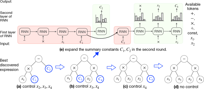
A.2 Concatenation-based Integration
The second possible idea is concatenating multiple layers of RNNs. The first layer of RNN is the trained RNN at the 1st round. We use the first layer of the RNN to take in the best sequence of the first round. When we read in a summary constant, we use the updated hidden vector of the first layer as the initial vector of the second layer RNN.
Take Figure 6 as an example. The first layer RNN takes the sequence . Because the 4th and 4th step input is summary constant type, we use the 4th and 5th step output vectors to initialize the hidden state vector of the second layer RNN. The second layer of RNN predicts two separated sub-expressions: and . The whole sequence corresponds to the sampled expression from the concatenated RNNs. The parameters inside the second layer RNN need to be trained by the policy gradient algorithm. Similarly, at the last round, we re-use pre-trained layers of RNN to take in the best-predicted expression and use one more layer to expand the summary constants in expression . The whole predicted sequence of tokens is the final predicted expression . Notice that the parameters of the prior layers of RNN can be frozen to reduce the number of parameters for training.
The main limitation of this idea is that: (1) we need to store all the trained RNNs. This does not scale up to many input variable cases. At the last round, we will have frozen layer of RNN and one trainable layer of RNN. (2) Due to multiple layers of RNNs and the sequence of input becoming longer and longer, then the training speed of the whole model will be slower and slower with fewer and fewer controlled variables.
Appendix B Extended Explanation of Vsr-Dpg method
Data-availability Assumption
A crucial assumption behind the success of vertical symbolic regression is the availability of a that returns a (noisy) observation of the dependent output with input variables in controlled. Such a data oracle represents conducting control variable experiments in the real world, which can be expensive. This differs from the horizontal symbolic regression, where a dataset is obtained prior to learning [49] with no variable controlled.
The vertical discovery path is to build algorithms that mimic human scientific discovery, which has achieved tremendous success in early works [40, 41, 42]. Recent work [50, 51, 52, 53] also pointed out the importance of having a data oracle that can actively query data points, rather than learning from a fixed dataset. In cases where it is difficult to obtain such a data oracle, Keren et al. proposed the use of deep neural networks to learn a data generator for the given set of controlled variables.
Objective and its Gradient
The loss function of Vsr-Dpg is informed by the REINFORCE algorithm [19], which is based on the log-derivative property: , where represents a probability distribution over input with parameters and notation is the partial derivative with respect to . In our formulation, let denote the probability of sampling a sequence of grammar rules and . Here is the corresponding expression constructed from the rules following the procedure in Section 3.1. the probability is modeled by The learning objective is to maximize the expected reward of the sampled expressions from the RNN:
Based on the REINFORCE algorithm, the gradient of the objective can be expanded as:
where represents all possible sequences of grammar rules sampled from the RNN. The above expectation can be estimated by computing the averaged over samples drawn from the distribution . We first sample several times from the RNN module and obtain sequences , an unbiased estimation of the gradient of the objective is computed as: . In practice, the above computation has a high variance. To reduce variance, it is common to subtract a baseline function from the reward. In this study, we choose the baseline function as the average of the reward of the current sampled batch expressions. Thus we have:
Based on the description of the execution pipeline of the proposed Vsr-Dpg, we summarize every step in Algorithm 1.
Implementation of Vsr-Dpg
In the experiments, we use Long short-term memory (LSTM) as the RNN layer and we configure the number of RNN layers as . The dimension of the input embedding layer and the hidden vector in LSTM is configured as 512. We use the Adam optimizer as the gradient descent algorithm with a learning rate of 0.009. The learning epoch for each round is configured 30. The maximum sequence of grammar rules is fixed to be . The number of expressions sampled from the RNN is set as 1024. When fitting the values of open constants in each expression, we sample a batch of data with batch size from the data Oracle. The open constants in the expressions are fitted on the data using the BFGS optimizer 111https://docs.scipy.org/doc/scipy/reference/optimize.minimize-bfgs.html. We use a multi-processor library to fit multiple expressions using 8 CPU cores in parallel. This greatly reduced the total training time.
An expression containing placeholder symbol or containing more than 20 open constants is not evaluated on the data, the fitness score of it is . In terms of the reward function in the policy gradient objective, we use . The normalized mean-squared error metric is further defined in Equation 3.
The deep network part is implemented using the most recent TensorFlow, the expression evaluation is based on the Sympy library, and the step for fitting open constants in expression with the dataset uses the Scipy library. Please find our code repository at: https://github.com/jiangnanhugo/VSR-DPG It contains 1) the implementation of our Vsr-Dpg method, 2) the list of datasets, and 3) the implementation of several baseline algorithms.
Appendix C Experiment Settings
C.1 Evaluation Metrics
The goodness-of-fit indicates how well the learning algorithms perform in discovering unknown symbolic expressions. Given a testing dataset generated from the ground-truth expression, we measure the goodness-of-fit of a predicted expression , by evaluating the mean-squared-error (MSE) and normalized-mean-squared-error (NMSE):
| MSE | (3) | |||
| NMSE |
The empirical variance . We use the NMSE as the main criterion for comparison in the experiments and present the results on the remaining metrics in the case studies. The main reason is that the NMSE is less impacted by the output range. The output ranges of expression are dramatically different from each other, making it difficult to present results uniformly if we use other metrics.
Prior work [10] further proposed coefficient of determination -based Accuracy over a group of expressions in the dataset, as a statistical measure of whether the best-predicted expression is almost close to the ground-truth expression. An of 1 indicates that the regression predictions perfectly fit the data [54]. Given a threshold value (we use ), for a dataset containing fitting tasks of expressions, the algorithm finds a group of best expressions correspondingly. The -based accuracy is computed as follows:
where and is an indicator function that outputs when the exceeds the threshold .
C.2 Symbolic Regression on Algebraic Equations
Baselines
We consider a list of current popular baselines based on genetic programming222https://github.com/jiangnanhugo/cvgp:
-
•
Genetic Programming (GP) maintains a population of candidate symbolic expressions, in which this population evolves between generations. In each generation, candidate expressions undergo mutation and crossover with a pre-configured probability value. Then in the selection step, expressions with the highest fitness scores (measured by the difference between the ground truth and candidate expression evaluation) are selected as the candidates for the next generation, together with a few randomly chosen expressions, to maintain diversity. After several generations, expressions with high fitness scores, i.e., those expressions that fit the data well survive in the pool of candidate solutions. The best expressions in all generations are recorded as hall-of-fame solutions.
-
•
Vertical symbolic regression with genetic programming (VSR-GP) builds on top of GP. It discovers the ground-truth expression following the vertical discovery path. In the -th round, it controls variables as constant, and only discovers the expression involving the rest variables .
Eureqa [46] is the current best commercial software based on evolutionary search algorithms. Eureqa works by uploading the dataset and the set of operators as a configuration file to its commercial server. This algorithm is currently maintained by the DataRobot webiste333https://docs.datarobot.com/en/docs/modeling/analyze-models/describe/eureqa.html. Computation is performed on its commercial server and only the discovered expression will be returned after several hours. We use the provided Python API to send the training dataset to the DataRobot website and collect the predicted expression from the server-returned result. For the Eureqa method, the fitness measure function is negative RMSE. We generated large datasets of size in training each dataset.
A line of methods based on reinforcement learning444https://github.com/dso-org/deep-symbolic-optimization:
-
•
Deep Symbolic Regression (DSR) [10] uses a combination of recurrent neural network (RNN) and reinforcement learning for symbolic regression. The RNN generates possible candidate expressions, and is trained with a risk-seeking policy gradient objective to generate better expressions.
-
•
Priority queue training (PQT) [16] also uses the RNN similar to DSR for generating candidate expressions. However, the RNN is trained with a supervised learning objective over a data batch sampled from a maximum reward priority queue, focusing on optimizing the best-predicted expression.
-
•
Vanilla Policy Gradient (VPG) [19] is similar to DSR method for the RNN part. The difference is that VPG uses the classic REINFORCE method for computing the policy gradient objective.
-
•
Neural-Guided Genetic Programming Population Seeding (GPMeld) [11] uses the RNN to generate candidate expressions, and these candidate expressions are improved by a genetic programming (GP) algorithm.
| (a) Genetic Programming-based methods. | |||
|---|---|---|---|
| VSR-GP | GP | Eureqa | |
| Fitness function | NegMSE | NegMSE | NegRMSE |
| Testing set size | |||
| #CPUs for training | 1 | 1 | N/A |
| #genetic generations | 200 | 200 | 10,000 |
| Mutation Probability | 0.8 | 0.8 | |
| Crossover Probability | 0.8 | 0.8 | |
| (b) Monte Carlo Tree Search-based methods. | |||
| MCTS | |||
| Fitness function | NegMSE | ||
| Testing set size | |||
| #CPUs for training | 1 | ||
| (c) Deep reinforcement learning-based methods. | |||
| DSR | PQT | GPMeld | |
| Reward function | 1/(1+NRMSE) | ||
| Training set size | |||
| Testing set size | |||
| Batch size | |||
| #CPUs for training | 8 | ||
| -risk-seeking policy | 0.02 | N/A | N/A |
| #genetic generations | N/A | N/A | 60 |
| #Hall of fame | N/A | N/A | 25 |
| Mutation Probability | N/A | N/A | 0.5 |
| Crossover Probability | N/A | N/A | 0.5 |
Symbolic Physics Learner (SPL) is a heuristic search algorithm based on Monte Carlo Tree Search for finding optimal sequences of production rules using context-free grammars [9, 8]555https://github.com/isds-neu/SymbolicPhysicsLearner. It employs Monte Carlo simulations to explore the search space of all the production rules and determine the value of each node in the search tree. SPL consists of four steps in each iteration: 1) Selection. Starting at a root node, recursively select the optimal child (i.e., one of the production rules) until reaching an expandable node or a leaf node. 2) Expansion. If the expandable node is not the terminal, create one or more of its child nodes to expand the search tree. 3) Simulation. Run a simulation from the new node until achieving the result. 4) Backpropagation. Update the node sequence from the new node to the root node with the simulated result. To balance the selection of optimal child node(s) by exploiting known rewards (exploitation) or expanding a new node to explore potential rewards exploration, the upper confidence bound (UCB) is often used.
End to End Transformer for symbolic regression (E2ETransformer) [39]666https://github.com/facebookresearch/symbolicregression. They propose to use a deep transformer to pre-train on a large set of randomly generated expressions. We load the shared pre-trained model. We provide the given dataset and the E2ETransformer infers 10 best expressions. We choose to report the expression with the best NMSE scores.
We list the major hyper-parameter settings for all the algorithms in Table 5. Note that if we use the default parameter settings, the GPMeld algorithm takes more than 1 day to train on one dataset. Because of such slow performance, we cut the number of genetic programming generations in GPMeld by half to ensure fair comparisons with other approaches.
Dataset for Algebraic Equations
The dataset is available at the code repository with the folder name:
.
The expressions used for comparison have the same mathematical operators . One configuration is shown in Table 6.
| Eq. ID | Exact Expression |
|---|---|
| prog-0 | |
| prog-1 | |
| prog-2 | |
| prog-3 | |
| prog-4 | |
| prog-5 | |
| prog-6 | |
| prog-7 | |
| prog-8 | |
| prog-9 |
For the extended analysis, where we consider many more input variables, they are available in the folder with the name:
where the value of is the number of total variables in, which can be .
The original expression is: . We extend this expression by choosing 5 variables from the total variables and mapping the selected variables to the variables . Here are 10 randomly generated expressions:
The rest expressions are available in the folder.
C.3 Symbolic Regression on Ordinary Differential Equations
The temporal evolution of the system is modeled by the time derivatives of the state variables. Let be the -dimensional vector of state variables, and is the vector of their time derivatives, which is noted as for abbreviation. The ordinary differential equation (ODEs) is of the form , where constant vector are parameters of the ODE model. Given the initial state , the finite time difference and the expression , the ODEs are numerically simulated to obtain the state trajectory , where and .
Task Definition
Following the definition of symbolic regression on differential equation in [45, 8], given a trajectory dataset of state variable and its time derivatives , represents the value of the derivative of variable at time , the symbolic regression task is to predict the best expression that minimizes the average loss on trajectory data:
Other formulations of this problem assume we have no access to its time derivatives, that is [47]. This formulation is tightly connected to our setting and relatively more challenging. We can still estimate the finite difference between the current and next state variables as its approximated time derivative: .
Baselines
For the baselines on the differentiable equations, we consider
-
•
SINDy [25]777https://github.com/dynamicslab/pysindy is a popular method using a sparse regression algorithm to find the differential equations.
-
•
ODEFormer [47]888https://github.com/sdascoli/odeformer is the most recent framework that uses the transformer for the discovery of ordinary differential equations. We use the provided pre-trained model to predict the governing expression with the dataset. We execute the model 10 times and pick the expression with the smallest NMSE error. The dataset size is , which is the largest dataset configuration for the ODEFormer.
-
•
ProGED [44]999https://github.com/brencej/ProGED uses probabilistic context-free grammar to search for differential equations. ProGED first samples a list of candidate expressions from the defined probabilistic context-free grammar for symbolic expressions. Then ProGED fits the open constants in each expression using the given training dataset. The equation with the best fitness scores is returned.
Dataset for Differential Equations.
We collect a set of real-world ordinary differential equations of multiple input variables from the SINDy codebase101010https://github.com/dynamicslab/pysindy/blob/master/pysindy/utils/odes.py.
-
•
Lorenz Attractor. Let be functions of time and stands for the position in the coordinates. Here we consider 3-dimensional Lorenz system whose dynamical behavior is governed by
with parameters .
-
•
Glycolysis Oscillations. The dynamic behavior of yeast glycolysis can be described as a set of 7 variables . The biological definition of each variable from Brechmann and Rendall is provided in Table 7. The governing equations are:
where the parameters . The rest of the differential equations from this Glycolysis family can be found at [55].
Variable Biological Definition Range Standard deviation Glucose Glyceraldehydes-3-phosphate and dihydroxyacetone phosphate pool 1,3-bisphosphoglycerate Cytosolic pyruvate and acetaldehyde pool NADH ATP Extracellular pyruvate and acetaldehyde pool Table 7: Biological definition of variables in Glycolysis Oscillations. The allowed range of initial states for the training data set and the standard deviation of the limit cycle are also included. -
•
MHD turbulence. The following equations describe the dynamic behavior of the Carbone and Veltri triadic MHD model:
where the parameters . [56] define as the velocity and as to the magnetic field. represents, respectively, the kinematic viscosity and the resistivity.
We notice there is a recently proposed dataset ODEBench [47]. It is not selected for study, since it mainly contains differential equations up to two variables.
Evaluation Metrics.
We use the -based Accuracy metric to evaluate if the whole set of predicted expressions has a score higher than .
Appendix D Extra Experiments
D.1 Discovered Algebraic Equations by each learning algorithm.
The predicted expression by Vsr-Dpg (ours) for configuration . 60% of the predicted expression has a NMSE score.
The predicted result for prog-0:
The predicted result for prog-1:
The predicted result for prog-2:
The predicted result for prog-3:
The predicted result for prog-4:
The predicted result for prog-5:
D.2 Discovered differential equations by each Learning Algorithm.
MHD turbulence
We collect the best-predicted expression by each algorithm.
SINDy.
ODEFormer
SPL
Vsr-Dpg (ours)