Reformulating polarized radiative transfer

The physical diagnosis of the solar atmosphere is achieved by solving the polarized radiative transfer problem for plasmas in Non-Local Thermodynamical Equilibrium (NLTE). This complex scenario poses theoretical challenges for integrating the radiative transfer equation (RTE) efficiently and demands better numerical methods for synthesis and inversion of polarization spectra. Indeed, the current theory and methods are limited to constant propagation matrices, thus imposing local solutions. To spark significant advances, we propose a formalism that reformulates the polarized transfer problem. Namely, this paper lays the foundations to achieve a non-local geometrical integration of the RTE based on the Magnus expansion. First, we revisit the statement of the problem and its general solutions in Jones and Stokes formalisms to clarify some inconsistencies in the literature, and to unify and update the nomenclature. Looking at both formalisms as equivalent representations of the Lorentz/Poincaré group of rotations, we interpret the RTE in terms of Lie group theory to remark the suitability of the Magnus expansion for obtaining accurate non-local solutions. We then present a detailed algebraic characterization of the propagation matrix involving a new generalized Lorentz matrix. Combining this, our ”basic evolution” theorem, and the Magnus expansion, we reformulate the homogenous solution to the RTE in Stokes formalism. Thus, we obtain the first compact analytical evolution operator that supports arbitrary spatial variations of the propagation matrix to first order in the Magnus expansion, paving the road to higher orders. Finally, we also reformulate the corresponding inhomogeneous solution as an exact equivalent homogeneous system, which is then solved analytically with the Magnus expansion. This gives the first efficient and consistent formal solution of the RTE that furthermore is non-local, natively accurate (prevents any numerical break down of the group structure of the solution), and that separates the integration from the formal solution. Such disruptive formulation leads to a new whole family of numerical radiative transfer methods and suggests accelerating NLTE syntheses and inversions with non-local radiative transfer. With minor cosmetic changes, our results are valid for other universal physical problems sharing the Lorentz/Poincaré algebra of the RTE and special relativity (e.g., motion of charges in inhomogeneous electromagnetic fields).

1 Introduction

Astrophysics studies the distant universe through light. Therefore, it is of upmost importance to have a precise understanding of how light is affected by different physical processes. In the framework of Maxwell’s electromagnetic wave theory, a light beam is fully characterized by the spectra of intensity and of polarization, as described either by the Stokes/Müller formalism or equivalently by the Jones formalism (Landi Degl’Innocenti & Landolfi, 2004; Stenflo, 1994). Currently, the measurement and interpretation of Stokes spectropolarimetry in atomic and molecular spectral lines is the preferred and best known way of diagnosing astrophysical plasmas. Namely, the Stokes vector is a practical and powerful way to describe any partially (i. e. naturally) polarized light beam by providing four vector components quantifying the number of photons and their direction of oscillation in the reference frame of the light beam and using common (intensity) units (Born & Wolf, 1980).

Having a way of quantifying polarization, the next step is to describe its transference through a plasma with the polarized radiative transfer equation (RTE). The best scenario to investigate this key astrophysical problem is the near solar atmosphere. In such a context with spatial resolution, radiative transfer is a fundamental part of the Non-Local Thermodynamical Equilibrium (NLTE) problem, in which radiation emitted at a given point modifies, via radiative transfer, the physical state of other distant points in the solar atmosphere. The polarized RTE contains a four-dimensional propagation matrix quantifying the microscopic physics through optical coefficients that depend on angle, wavelength, and distance along the ray. This makes the integration of the RTE the most frequent and complex operation carried out in NLTE iterative schemes, specially when considering multidimensional solar models. One of the motivations for the present paper is to accelerate the NLTE calculations by solving the RTE with more consistent, robust, and accurate methods. But this implies to beat a more fundamental goal: solving the RTE consistently in spatially resolved solar models without assuming constant local properties. Let us see why this is the next frontier in polarized radiative transfer.

After Unno (1956) pioneered the first derivation of the RTE accounting for magnetic fields,  Rachkovsky (1967) completed the equation and gave a first analytical solution valid for spatially homogeneous (Milne-Eddington) atmospheres with constant propagation matrix. Later, van Ballegooijen (1985) and Landi Deglinnocenti & Landi Deglinnocenti (1985) provided specific evolution operators solving the homogeneous RTE with constant spatial properties. However, spatial variations are not negligible in the solar atmosphere. Soon it was known that the numerical solutions of the RTE improved when subdividing the atmosphere into numerous layers (e.g., Rees et al., 1989; Bellot Rubio et al., 1998) and the need for models with spatial variations was confirmed by numerical inversions of observed solar Stokes profiles (Collados et al., 1994; Del Toro Iniesta & Ruiz Cobo, 1996).

At the beginning, the inhomogeneous character of the solar atmosphere was mainly attributed to the large-scale stratification in density, temperature, and magnetic field. However, the evolution of telescopes and simulations has also shown omnipresent small-scale variations. In particular, synthetic MHD solar models started to support large inhomogeneity due to macroscopic motions, especially in the dynamic chromosphere (e.g., Carlsson & Stein, 1997). Indeed, plasma velocity gradients in sound/shock waves are main sources of solar small-scale variations and discontinuities, having a large and specific impact in the polarization via radiative transfer effects (Carlin et al., 2013), either due to their modulation of radiation field anisotropy (Carlin & Asensio Ramos, 2015) and/or due to a relatively new phenomenon that we call dynamic dichroism (Carlin, 2019).

In order to cope with spatial atmospheric variations in resolved atmospheres with formalisms based on constant properties, strategies such as ”ray characteristics” (e.g., Kunasz & Auer, 1988) and several integration numerical methods have been developed. Some of the most representative are: the piecewise constant Evolution Operator method (van Ballegooijen, 1985; Landi Deglinnocenti & Landi Deglinnocenti, 1985, hereafter vB85 and LD85), the “DELO” methods (Rees et al., 1989) of linear, semi- parabolic, and parabolic kind (see Janett et al., 2017, and references therein); and the order-3 DELO-Bezier (De la Cruz Rodríguez & Piskunov, 2013) and Hermite (Bellot Rubio et al., 1998) methods. Numerically, these schemes are considered advantageous against older standards, such as the diagonalization of the propagation matrix (Šidlichovsky,1976) or the Runge-Kutta scheme, which demands a too large number of grid points controlled by the eigenvalues of the propagation matrix (Landi Degl’Innocenti, 1976).

Hence, despite nowadays we know that both large and small scale spatial variations are needed to represent stellar atmospheres, all existing numerical methods for solving the polarized RTE in solar physics and astrophysics remain limited to constant spatial properties. The bottleneck is in a theory based on an evolution operator constrained to constant propagation matrix. Thus, in order to approach the limit of constant properties in every numerical cell, the current methods demand to sequentially solve the RTE many times along every ray. This process scales with the resolution of the models, becoming a main source of computational cost. In addition, the approach cannot be exact because the limit of constant properties is never fully achieved due to the fact that the radiative transfer depends on several atmospheric physical quantities with different sources of gradients and scales of variation. Furthermore, it cannot be achieved simultaneously and equally for all wavelengths (e.g.around a spectral line) because the integration step of any numerical cell change with wavelength (e.g. because opacity does it). This fact is reinforced by the sensitivity of the optical depth step to Doppler shifts and opacity variations in the atmospheres.

Another issue that is never mentioned is that current methods propagate the physical solution along the light beam by imposing an emissivity that does change continuously while the propagation matrix is locally constant, which is inconsistent. Physically, it is incorrect because emissivity cannot change if the propagation matrix is constant, but it also corrupts indirectly the mathematical meaning of the RTE by breaking its Lie group structure. In other words, current methods are actually not solving the target physical problem, but a different one.

For reasons like these, it should be expected that the numerical properties of current methods are limited by construction: they are not designed for spatial variations. Obviously, all this has negative consequences in the more general NLTE problem. In the work starting here, we clarify these limitations while moving to the real case in which arbitrary spatial variations can be consistently accounted in the RTE. Until now, the only attempt to solve this general problem was made by Semel & López Ariste (1999) and  López Ariste & Semel (1999), hereafter SLA99 and LAS99. Considering the group structure of the RTE, they applied the Wei & Norman (1963) method to formally pose a non-local evolution operator based on products of exponentials. However, their formulation does not provide a closed formula for the radiative transfer solution and demands to solve several differential equations for the optical coefficients of the RTE, such that they did not materialize it numerically arguing that it would not be economic. Without discarding their results, which will be compared with ours a posteriori, we present a different approach.

Here we must mention the key problem of commutativity: when an atmosphere varies spatially, its propagation matrices do not generally commute between points, which complicates an exact solution. SLA99 saw this as a limitation, arguing that, without commuting layers, the solution requires constant propagation matrices and forces a discretization of the atmosphere. In our work, we assume a discretization and arbitrary spatial variations as requirements. Consequently, we fully embrace non-commutativity as part of the problem, posing the foundations to incorporate it in the theory. To do this, we use the Magnus expansion (Magnus, 1954), an approach that SLA99 explicitly intended to avoid due to its complexity. Among its several remarkable aspects (e.g., Blanes et al., 2009), this object preserves the algebraic group structure and intrinsic properties of the exact solution after truncation in the algebra of a Lie group. As will be seen later, its group elements are neatly defined with a single exponential, thus avoiding products of exponentials, differential formulations, and (inexact) perturbative developments.

This paper has to be understood as the first of a series where we reformulate the radiative transfer problem with the Magnus expansion. Here, we present the general theory of our formalism:

1) In Section 2, we re-derive the RTE and its general solutions both in Stokes and Jones formalisms, using a common framework and nomenclature and stating some relations that are unclear in the literature. This introductory step is also necessary to motivate the future extension of our approach to the Jones formalism, where the solution and the Magnus expansion could adopt an advantageous analytical form.

2) In section 3, we set a minimal framework to work with Lie group rotations, showing the limitations of current evolution operators, and introducing the Magnus solution and our Basic Evolution theorem to solve the exact exponential of any integral of the propagation matrix.

3) Section 4 combines some aspects of Lie group representation and multidimensional rotations, leading to a detailed characterization of the propagation vector and the propagation matrix.

5) In Section 5, we calculate our compact analytical evolution operator using the Magnus solution to first order.

6) Finally, Section 6 reformulates and calculates the inhomogeneous formal solution in Stokes formalism.

2 A brief description of natural polarized light

Electromagnetic waves travel along the direction of propagation $\mathbf{k}=\mathbf{E}\times\mathbf{B}$, as the electric field oscillates and rotates in the plane $\Pi\bot\mathbf{k}$. We adopt a right-handed reference system $(\hat{{\bm{e}}}_{1},\hat{{\bm{e}}}_{2},\mathbf{k})$ with two perpendicular unit vectors $\hat{{\bm{e}}}_{1}$ and $\hat{{\bm{e}}}_{2}$ contained in $\Pi$. Natural light is then described as an incoherent superposition of waves in a wave packet constrained to a small range of wavenumbers ${\bm{\Delta}\bm{k}}$ around $\mathbf{k}$, hence having a finite but small (quasi-monochromatic) frequency bandwidth $\Delta\omega\approx c|{\bm{\Delta}\mathbf{k}}|$ and an angular spread in the solid angle $\Delta\Omega\approx|{\bm{\Delta}}\mathbf{k}|/\mathbf{k}$. Integrating in ${\delta\bm{k}}$ all waves in the range ${\bm{\Delta}\bm{k}}$, the total electric oscillation at any point P in $\Pi$ is:

$$\centering\mathbf{E}(P,t)=\rm{Re}\,\left[\left(\mathcal{E}_{1}(P,t)\,\hat{\mathbf{e}}_{1}+\mathcal{E}_{2}(P,t)\,\hat{\mathbf{e}}_{2}\right)\,e^{\pm i(\mathbf{k}\cdot\mathbf{r_{P}}-\omega t)}\right],\@add@centering$$ (1)

where

$$\centering\mathcal{E}_{i}(P,t)=\int\rm{d}^{3}(\delta\mathbf{k})\,n(\delta\mathbf{k})\,E_{i}(\mathbf{k}+\delta\mathbf{k})\,e^{\pm i(\phi_{i}+\delta\mathbf{k}\cdot\mathbf{r_{P}}-\delta\omega\,t)}\@add@centering$$ (2)

are the total complex electric field amplitudes of the wave packet along each reference axis, while $E_{i}(\mathbf{k}+\delta\mathbf{k})$ and $\phi_{i}$ are the corresponding real electric amplitudes and phases for every single wave with wavenumber $\mathbf{k^{\prime}}=\mathbf{k}+\delta\mathbf{k}$ and angular frequency $\omega+\delta\omega=c|\mathbf{k^{\prime}}|$. Finally, $n(\delta\mathbf{k})$ is the number density of waves in the three-dimensional wavenumber space.

Two signs are possible in the above exponentials. Following Landi Degl’Innocenti & Landolfi (2004), we choose as convention the positive sign (i.e., negative temporal exponent).

With products of the electric amplitudes given by Eq. (2) we can define the average polarization tensor $J_{ij}$. From it, we also define the Stokes vector $\@vec{I}=(I,Q,U,V)^{\intercal}$, which quantifies the observable properties of the average polarization ellipse produced by the total electric field vector oscillating in $\Pi$. These two quantities are related as ($u$ is a constant converting from squared electric field to intensity units):

$$\@vec{J}=u\cdot\left(\begin{array}[]{cc}<\mathcal{E}^{*}_{1}\mathcal{E}_{1}>&<\mathcal{E}^{*}_{1}\mathcal{E}_{2}>\\ <\mathcal{E}^{*}_{2}\mathcal{E}_{1}>&<\mathcal{E}^{*}_{2}\mathcal{E}_{2}>\end{array}\right) =\frac{1}{2}\cdot\left(\begin{array}[]{cc}I+Q&U-iV\\ U+iV&I-Q\end{array}\right)$$ (3e)

$$I =J_{11}+J_{22},\quad\quad Q=J_{11}-J_{22},$$

$$U =J_{12}+J_{21},\quad\quad V=i\,(J_{12}-J_{21}),$$ (3f)

Thus, a light beam propagating along $\mathbf{k}$ has a total number of photons quantified by Stokes I, a linear polarization defined by both Stokes Q and U along two reference directions in $\Pi$, and a circular polarization given by Stokes V, which is the difference between right-handed and left-handed circularly polarized photons using $\mathbf{k}$ as reference direction. Hence, Stokes V quantifies the rotation of the electric field vector around $\mathbf{k}$. By convention, it is defined positive/negative when that field is seen rotating clockwise/counter-clockwise from the observer (right-handed/left-handed circular polarization).

A consequence of considering a realistic superposition of quasi-monochromatic waves to quantify polarization is that the ideal physical relation $I^{2}=Q^{2}+U^{2}+V^{2}$, holding for a monochromatic wave, is substituted by the constrain:

$$I^{2}>Q^{2}+U^{2}+V^{2}\quad\quad(|\@vec{J}|\neq 0).$$ (4)

Equation (4) defines the Poincaré sphere by mapping the Stokes vector with points in the three-dimensional space $Q/I,U/I,V/I$ (Shurcliff, 2013). The polarization degree is the radius of such sphere $p=\sqrt{Q^{2}+U^{2}+V^{2}}/I<1$, meaning that the wave packet has become partially polarized because there are photons that do not contribute to Q, U or V.

2.1 The evolution equation for polarized radiation

We now consider a general atmosphere with different complex refractive indices $n_{\alpha}$ along each perpendicular spatial direction $\alpha$ in an atmosphere reference frame. From Eq.(1), one can then derive the spatial evolution of the transverse components of the electric field for a stationary quasi-monochromatic wave in our basis $(\hat{{\bm{e}}}_{1},\hat{{\bm{e}}}_{2},\mathbf{k})$ as a function of the optical properties of the medium, and from there the components $J_{ij}$ in Eq.(3e). Assuming the physical conditions associated to astrophysical plasmas (natural light in linear optics regime), and calling $s$ the geometrical distance along the ray $\mathbf{k}$, the result is (Landi Degl’Innocenti & Landolfi, 2004, Sect. 5.2) :

$$\frac{{\rm d}J_{ij}}{\rm{ds}}=-\sum^{2}_{k=1}(P^{*}_{ik}J_{kj}+P_{jk}J_{ik}),\quad(i,j=1,2)$$ (5)

where the propagation tensor is $P_{jk}=-ikg^{\alpha}_{jk}n_{\alpha}$ with real and imaginary parts $\bar{P}_{jk}+i\breve{P}_{jk}$. However, in astrophysics we use optical coefficients instead of the propagation tensor. We have found the following succint relations holding between them:

$$\eta_{I} =P^{*}_{11}+P^{*}_{22},\quad\quad\eta_{Q}+i\rho_{Q}=P^{*}_{11}-P^{*}_{22},$$ (6a)

$$\eta_{U}+i\rho_{U} =P^{*}_{12}+P^{*}_{21},\quad\quad\eta_{V}+i\rho_{V}=i(P^{*}_{12}-P^{*}_{21}),$$ (6b)

where we shall call propagation vector to that with components:

$$a_{k}=\eta_{k}+i\rho_{k},\quad\quad k=\mathrm{1,2,3}$$ (7)

Hereafter, $k=0,1,2,3$ refer to quantities associated to Stokes vector components $I,Q,U,V$. Thus, the above coefficients describe total absorption ($\eta_{0}$), dichroism ($\eta_{1,2,3}$) and anomalous dispersion ($\rho_{1,2,3}$) for the corresponding Stokes parameter. Since light propagates through an anisotropic plasma while oscillating transversally, the complex components of the electric field, $\varepsilon_{1}$ and $\varepsilon_{2}$, find different refraction indexes along the transfer, which explains the meaning of each optical coefficient..

The RTE is completed adding to Eq.(5) a term with emissivity coefficients $\epsilon_{0,1,2,3}$ quantifying the sources of photons. The emissivity and the seven propagation coefficients are involved functions of wavelength, propagation angle, and other parameters defining the micro-physics of the atmosphere (temperature, velocity, density, and magnetic field). We shall assume them already calculated for every wavelengh and spatial point along a given ray of light.

2.2 Radiative transfer equation in the Jones formalism

Developing Eq.(5), adding the source term, and considering the relations in Eqs.(3) and (6), we obtain the RTE in terms of 2x2 matrices (Jones formalism; see Shurcliff, 2013):

$$\frac{\rm{d}}{\rm{ds}}\@vec{J}=\@vec{E}-(\tilde{\@vec{K}}\@vec{J}+\@vec{J}\tilde{\@vec{K}}^{+}),$$ (8)

where the emissivity term is

$$\@vec{E}=\frac{1}{2}\cdot\left(\begin{array}[]{cc}\epsilon_{I}+\epsilon_{Q}&\epsilon_{U}-i\epsilon_{V}\\ \epsilon_{U}+i\epsilon_{V}&\epsilon_{I}-\epsilon_{Q}\end{array}\right),$$ (9)

the 2x2 propagation matrix is:

$$\tilde{\@vec{K}}=\frac{1}{2}\cdot\left(\begin{array}[]{cc}\eta_{I}+a_{Q}&a_{U}-ia_{V}\\ a_{U}+ia_{V}&\eta_{I}-a_{Q}\end{array}\right).$$ (10)

and $\@vec{J}$ was written in terms of the Stokes parameters in Eq.(3e).

These equations differ from those in van Ballegooijen (1985) (also Kalkofen, 1987) in some aspects. First of all, we use a more convenient, modern and general nomenclature. Namely, we do not constrain the equations to the particular geometry of a stratified atmosphere, we use geometrical distance along the optical path instead of optical depth as the evolution parameter, and we do not assume yet any particular expressions for the optical coefficients, allowing to represent any general physical situation to describe the plasma element (e.g. to consider scattering polarization, Hanle physics, etc.). Secondly, we use the definition $a_{k}=\eta_{k}+i\rho_{k}$ in Eq. (7), instead of the frequency profiles associated to $\eta_{k}-i\rho_{k}$, to obtain compact and cleaner expressions. This also allows us to present similar treatments for both Stokes and Jones formalisms and thus compare them using similar quantities agreeing with the monograph of Landi Degl’Innocenti & Landolfi (2004).

Finally, with respect to vB85’s, our expressions have non-obvious sign differences in all $\epsilon_{V}$, $a_{V}$, and Stokes $V$, which demands an explanation. The convention of signs mentioned after Eq. (2) for the temporal exponentials of the electric field sets the handedness (sign) of Stokes V: inverting the convention is equivalent to complex conjugation in the polarization tensor and therefore in Stokes V, as obvious from Eqs. (3). Despite vB85’s specifies our same (right-handed) basis for the electric field, that author does not specify a sign convention. A direct calculation shows that the sign differences comes from that issue, and that our choice leads to the same $2\times 2$ system of matrices if $a_{k}$ is defined as we did. In summary, one convention corresponds to our equations, while the other one uses instead $a_{k}=\eta_{k}-i\rho_{k}$ and negative signs for the exponentials in Eqs. (1) and (2). These latter choice would imply doing $\@vec{J}\rightarrow\@vec{J}^{*}$, $iV\leftrightarrow-iV$, $ia_{V}\leftrightarrow-ia_{V}$, and $i\epsilon_{V}\leftrightarrow-i\epsilon_{V}$ in our Jones formulation.

2.3 Radiative transfer equation in Stokes formalism

Carrying out the matrix products in Eq.(8) and separating real and imaginary parts, we obtain the polarized RTE in Stokes’ formalism. It is a system of four coupled first-order, ordinary differential equations whose homogeneous/inhomogeneous term contains the propagation/emissivity matrix/vector (e.g., Landi Degl’Innocenti & Landolfi, 2004, chapter 8):

$$\centering\frac{\rm{d}}{\rm{ds}}{\bf I}={\bm{\epsilon}}-{\bf KI},\@add@centering$$ (11)

with ${\bm{\epsilon}}$ the emissivity vector and ${\bf K}$ the 4x4 propagation matrix:

$$\centering\frac{\rm{d}}{\rm{ds}}\left(\begin{array}[]{c}I\\ Q\\ U\\ V\end{array}\right)=\left(\begin{array}[]{c}\epsilon_{I}\\ \epsilon_{Q}\\ \epsilon_{U}\\ \epsilon_{V}\end{array}\right)-\left(\begin{array}[]{cccc}\eta_{I}&\eta_{Q}&\eta_{U}&\eta_{V}\\ \eta_{Q}&\eta_{I}&\rho_{V}&-\rho_{U}\\ \eta_{U}&-\rho_{V}&\eta_{I}&\rho_{Q}\\ \eta_{V}&\rho_{U}&-\rho_{Q}&\eta_{I}\end{array}\right)\left(\begin{array}[]{c}I\\ Q\\ U\\ V\end{array}\right).\@add@centering$$ (12)

The Stokes and Jones formalisms are equivalent in that they describe the same physical problem (e.g., Sanchez Almeida, 1992). The fact that one can derive the Stokes RTE from Jones’ proves this. Historically, the solar and astrophysical community has preferred the Stokes formalism. The reason to include them both in this first paper is to facilitate a posterior comparison from the standpoint of our formulation, because the algebraic properties of the Jones $2\times 2$ matrices could imply advantages when working with the Magnus expansion.

2.4 Generic solution in Jones formalism

In order to solve the RTE, one first consider its homogeneous part, i.e. the RTE without emissivity, and then use it to solve the inhomogeneous part. For the Jones formalism, we follow a derivation similar to that of vB85, but adapting it to our general nomenclature and adding small improvements. First, we assume an homogeneous solution to Eq. (8) as the following variation of a certain auxiliar $\@vec{J}_{\rm a}$ along the trajectory parameter s:

$$\begin{split}\@vec{J}(s)=&\mathrm{\mathbf{O}}(s,s_{0}){\@vec{J}_{\rm a}}(s)\rm{\mathbf{O}}^{\dagger}(s,s_{0}),\end{split}$$ (13)

where the evolution operator $\mathrm{\mathbf{O}}\equiv\mathrm{\mathbf{O}}(s,s_{0};\breve{\rm{\mathbf{K}}})$ is a $2\times 2$ complex matrix fulfilling:

$$\frac{d{\mathbf{O}}}{ds}=-\breve{\rm{\mathbf{K}}}(s){\mathbf{O}},\quad\quad\left(\Rightarrow\frac{d{\rm{\mathbf{O}}^{\dagger}}}{ds}=-{\rm{\mathbf{O}}^{\dagger}}\breve{\rm{\mathbf{K}}}^{\dagger}(s)\right),$$ (14)

Differentiating Eq. (13) with respect to $s$, substituting $\@vec{J}$ and its derivative in Eq. (8), and removing terms cancelling each other, we obtain:

$$\frac{d\@vec{J}_{\rm a}(s)}{ds}=\mathrm{\mathbf{O}^{-1}}\mathbf{E}(s)\,[\rm{\mathbf{O}}^{-1}]^{\dagger},$$ (15)

whose integral

$$\@vec{J}_{\rm a}(s)=\@vec{J}_{\rm a}(s_{0})+\int^{s}_{s_{0}}{ds^{\prime}}\mathrm{\mathbf{O}^{-1}}(s^{\prime},s_{0})\mathbf{E}(s^{\prime})\,[\rm{\mathbf{O}}^{-1}]^{\dagger}(s^{\prime},s_{0}),$$ (16)

is then inserted into Eq. (13). Now, we improve the result of vB85 by specifying the boundary term and combining evolution operators to the left and to the right into a total evolution operator $\mathrm{\mathbf{O}_{T}}$. Thus, we obtain our generic inhomogenous solution in Jones formalism:

$$\centering\@vec{J}(s)=\@vec{J}(s_{0})+\int^{s}_{s_{0}}ds^{\prime}\mathrm{\mathbf{O}_{T}}(s,s^{\prime})\mathbf{E}(s^{\prime})\,\rm{\mathbf{O}^{\dagger}_{T}}(s,s^{\prime}),\@add@centering$$ (17)

where

$$\mathrm{\mathbf{O}_{T}}(s,s^{\prime})=\mathrm{\mathbf{O}}(s,s_{0})\cdot\mathrm{\mathbf{O}^{-1}}(s^{\prime},s_{0}).$$ (18)

and where the first term is the boundary contribution, which in analogy with Eq.(13), has been called

$$\@vec{J}(s_{0})=\mathrm{\mathbf{O}}(s,s_{0})\@vec{J}_{\rm a}(s_{0})\,\rm{\mathbf{O}}^{\dagger}(s,s_{0}).$$ (19)

VB85 did not specify the boundary term because applied the solution to an optically thick atmosphere as a whole piece, in which case the boundary term cancels out due to the physical properties of the boundaries (zero illumination for incoming rays and optically thick atmosphere for emerging rays). But in practice, the atmosphere is discretized and the integrals are applied sequentially to every cell of a reduced physical domain that is optically thin. Hence, we need to retain and specify the changing boundary contribution for each step. Note that in Eq. (17) the total solution is the direct addition of an integral to the previous solution at the boundary, without multiplying the latter by an evolution operator as in the Eq. (23) of the Stokes formalism.

2.5 Generic solution in Stokes formalism

From Eq.(11), the homogenous RTE in Stokes formalism is posed as the initial value problem:

$$\frac{d\mathbf{I}(s)}{ds}=-\mathbf{K}(s)\mathbf{I}(s);\quad\quad\mathbf{I}(s_{0})=\mathbf{I}_{0},$$ (20)

Integrating in an interval $\rm\Delta s=s-s_{0}$, its homogeneous formal solution is given by an evolution operator $\mathbf{O}(s,s_{0};\mathbf{K})$ applied to the initial value

$$\mathbf{I}(s)=\rm{\mathbf{O}}(s,s_{0};{\bf K})\cdot\mathbf{I}(s_{0}),$$ (21)

with $\rm{\mathbf{O}}^{s}_{s_{0}}\equiv\rm{\mathbf{O}}(s,s_{0};{\bf K})$ being solution to

$$\begin{split}\frac{d}{ds}{\mathbf{O}}^{s}_{s_{0}}=-\rm{\mathbf{K}}(s){\mathbf{O}}^{s}_{s_{0}},\quad\quad{\mathbf{O}}^{s_{0}}_{s_{0}}=\mathbbold{1}\end{split}$$ (22)

Once the evolution operator is known, the general formal inhomogenous solution to the RTE is posed

$$\mathbf{I}(s)=\rm{\mathbf{O}}(s,s_{0})\mathbf{I}(s_{0})+\int^{s}_{s_{0}}ds^{\prime}\rm{\mathbf{O}}(s,s^{\prime}){\bm{\epsilon}}(s^{\prime}).$$ (23)

The suitability of this solution is physically and numerically determined by the specific expressions adopted for the evolution operator and for the above integral. In the following sections, we will both reformulate the evolution operator and the inhomogeneous solution to develop better ways of solving the RTE.

3 Foundations for reformulating the radiative transfer solution with the Magnus expansion

In astrophysics, the term evolution operator has been used to refer both to a very general concept and to very particular methods, which is confusing. The concept was originally known in matrix theory as the matricant (Gantmacher, 1959), and refers to the matrix advancing the solution of a differential equation along a trajectory of integration. For instance, in Stokes formalism, Eq. (21) defines the evolution operator as the $4\times 4$ real matrix that, when multiplied by the Stokes vector at $s_{0}$, gives the Stokes vector solution at point $s$. Therefore it fully characterizes the final solution, both physically and numerically.

Instead, the methods associated to the evolution operator were introduced in solar physics by vB85 (see also Kalkofen, 2009) and later by LD85 to approximate explicit analytical evolution operators for the RTE in the Jones and Stokes formalism, respectively. Essentially, these methods consists in conveniently decomposing a constant propagation matrix to approximate its exponential. Thereafter, a numerical representation of it can be implemented to obtain the inhomogeneous solution for the transfer between $s_{0}$ and $s$ from Eqs. (23) or (17). Thus, to solve them we need an explicit expression for the evolution operator (homogeneous solution), and a way of solving the integrals (inhomogeneous solution).

The numerical approximations to the evolution operator are apparently easier than the analytical ones in their formulation, which made them dominate in our field. However, an analytical approach as the one we are going to develop can lead to more accurate numerical implementations because part of the result has been already calculated analytically and exactly. Furthemore, it allows to study the theoretical dependence of the solution on some parameters. The key to develop a suitable analytical solution that can later be translated into a powerful numerical method is to respect the Lie group structure of the RTE, which preserves the qualitative properties of the exact solution. As part of the foundations supporting our work with the Magnus expansion, we present now a brief conceptual framework to interpret the evolution of the solution to the RTE from the point of view of Lie groups.

In particular, a Lie group is a group of elements with a main group operation mapping its elements smoothly to form a differentiable manifold $\mathcal{M}$ (topological condition), but also fulfilling an algebraic condition: the result of combining the elements of $\mathcal{M}$ together with the operation of commutation stays in $\mathcal{M}$. The interest in Lie groups for solving differential equations is that being differentiable, hence analytical, there exists tangents to them at any point $p\in\mathcal{M}$.

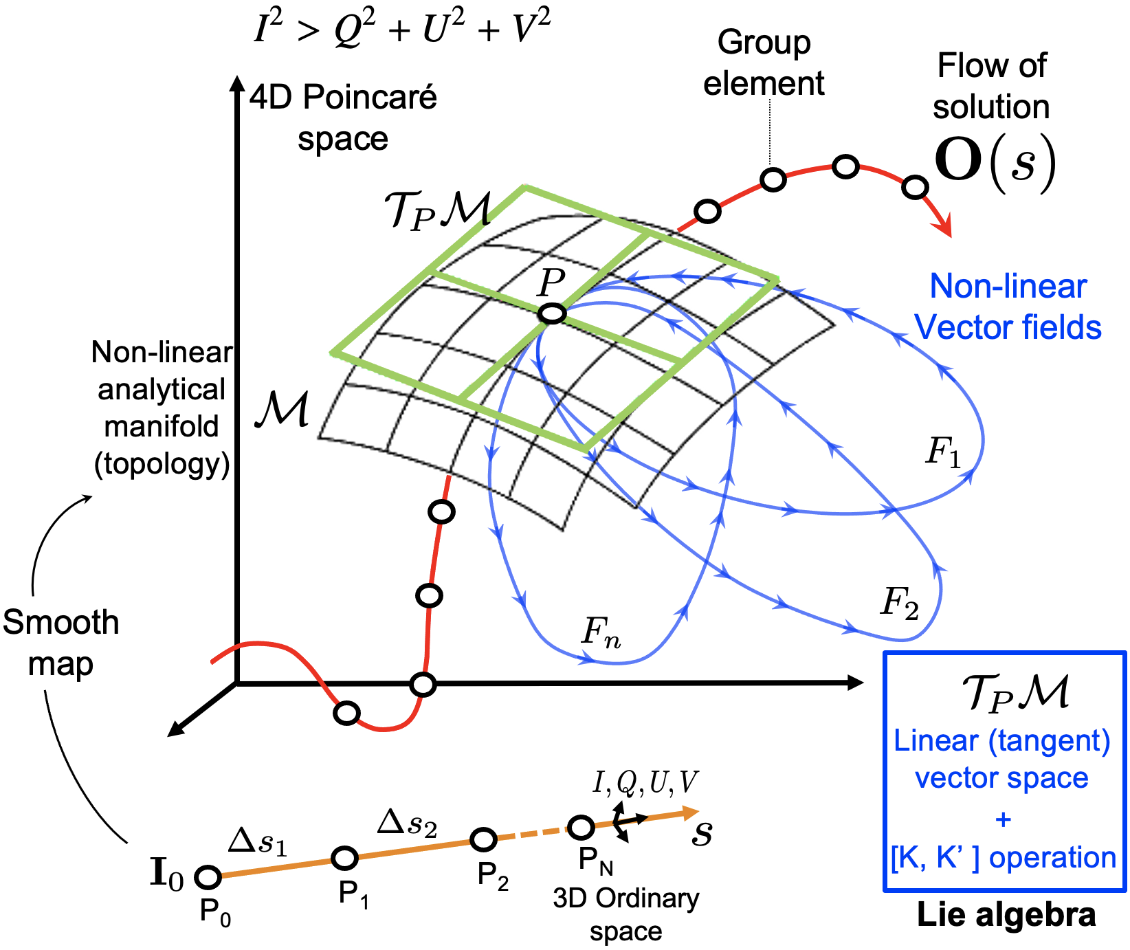
Figure 1: Solution to the RTE evolving in the ordinary 3D space of the ray (orange) and in the 4D space of the Poincaré group (red). A local solution (white circles) is an element of the Lie group and an exponential map of vector fields (blue) associated to the corresponding Lie algebra.

$\begin{array}[]{ccc}\includegraphics[scale={0.272}]{f1a.png}&\includegraphics[scale={0.245}]{f1b.png}&\includegraphics[scale={0.25}]{f1c.pdf}\\ \end{array}$

Figure 2: Examples of basic vector fields (arrows) and corresponding flow solutions (red lines) to the homogeneous RTE for different wavelengths. Left: rotational flow due to magneto-optical effects for constant $\mathbf{K}$ in plane Q-U. The trajectory, which should be circular, deviates to describe a spiral due to the accumulated inaccuracy error in the standard integration method employed here. Middle: hyperbolic flow due to dichroism in I-V plane for constant $\mathbf{K}$. Right: combination of vector fields and evolution of solution in QUV space for non-constant $\mathbf{K}$.

A tangent vector at $p$ can be defined by differentiating a smooth parametric curve $\gamma(s)$ such that $\gamma(0)=p$ (e.g., Bonfiglioli & Fulci, 2011):

$$\bm{v}=\left.\frac{d\gamma(s-s_{0})}{ds}\right|_{s=s_{0}}$$ (24)

As illustrated in Fig. 1, the set of all possible tangent vectors at $p$ forms the linear vector space $\mathcal{T}$ (the tangent space of the group). If locally (in the neighourghood of each $p$) we associate $\gamma(s)$ with the evolution of the solution to a linear ODE on $\mathcal{M}$, then the infinitesimal advance of the solution at $p$ occurs in a direction contained in its tangent space. Hence, instead of working in the non-linear manifold $\mathcal{M}$, Lie groups offer the mathematical foundation for solving the ODE in a linear vector space while preserving the local structure of the group.

The key to do this is that the elements in $\mathcal{M}$ can also be obtained by mapping (e.g., exponentiating) those of the so-called Lie algebra $\mathfrak{g}$ of the group. The algebra is defined as the combination of the tangent vector space around the group identity element with the operation of commutation. In that way, the algebraic structure of a Lie group is captured by its Lie algebra, a simpler object (since it is a vector space).

To particularize these basic ideas, consider the homogeneous RTE and its formal solution in Stokes formalism given by Eqs. (20) and (21) with system matrix $\mathbf{A}=-\mathbf{K}$:

$$\bm{I}^{\prime}(s)=\mathbf{A}(s)\bm{I}(s);\quad\quad\bm{I}(s_{0})=\bm{I}_{0},$$ (25)

$$\bm{I}(s)=\mathbf{O}(s,s_{0};\mathbf{A})\bm{I}_{0}.$$ (26)

As the l.h.s. of the RTE is a first derivative with respect to $s$, $\mathbf{A}$ can be seen as a vector field tangent to the s-parametric streamline followed by the system when transiting from $\bm{I}(s_{0})$ to $\bm{I}(s)$ in $\mathcal{M}$, while the evolution operator $\mathbf{O}(s,s_{0};\mathbf{A})$ is called the flow of $\mathbf{A}$ because it advances the solution following $\mathbf{A}$. The matrix $\mathbf{A}$ represents a vector field (a.k.a. infinitesimal generator) when is seen as the derivative of the flow at $s=s_{0}$:

$$\mathbf{A}=\left.\frac{d\mathbf{O}(s,s_{0};\mathbf{A})}{ds}\right|_{s=s_{0}}.$$ (27)

This operation represents a local coordinate map between the elements of the group and its tangent linear space $\mathcal{T}$ formed by the set of all possible vector fields $\mathbf{A}$. Namely, one can see that such a coordinate map is possible at the identity of the group, i.e. where $\bm{O}(s,s_{0};\mathbf{A})=\mathbbold{1}$ in $s=s_{0}$. In general, this condition is satisfied if the evolution operator is an exponential map. Then, as commutators of system matrices at points nearby the identity element $([\mathbf{A}_{1},\mathbf{A}_{2}]=\mathbf{A}_{1}\mathbf{A}_{2}-\mathbf{A}_{2}\mathbf{A}_{1}$) represent the total derivative of the vector field $\mathbf{A}$ in $\mathfrak{g}$, their exponentiation is equivalent to infinitesimal translations in the group. A more specific representation of the evolution of the solution to the RTE in terms of vector fields and flows is presented in Fig. 2(see caption).

In the rest of this section we make the evolution operator more explicit. As it is formally the same in both the Stokes and Jones formalisms, we shall focus in the former.

3.1 The universal solution to the evolution operator is a series

In general, the evolution operator solving the homogeneous RTE in Eq. (25) is given by the Volterra (1887)’s integral equation

$$\begin{split}&\mathbf{O}(s,s_{0};\mathbf{A})=\mathbbold{1}+\int^{s}_{s_{0}}dt\mathbf{A}(t)\mathbf{O}(t,s_{0},\mathbf{A}),\\ \end{split}$$ (28)

after applying the fundamental theorem of calculus to Eq.(26) with $O(s_{0},s_{0})=\mathbbold{1}$. A Picard iteration on Eq. (28) can start with $O(t,s_{0},A)=0$ and be continued up to infinity. Thus, an expression for $O(s,s_{0})$ was first obtained by Peano (1888) (also Peano (1890) or translation in Kannenberg (2000)) and further studied by Baker (1902, 1905). It is the funny Peano-Baker series:

$$\begin{split}&\mathbf{O}(s,s_{0};\mathbf{A})=\mathbbold{1}+\mathrm{H\mathbf{A}+H\mathbf{A}H\mathbf{A}+H\mathbf{A}H\mathbf{A}H\mathbf{A}}+\ldots\\ \end{split}$$ (29)

where $\rm H\mathbf{A}$ is the result of applying the integral operator $H$ for integrating the matrix $\mathbf{A}=(a)_{ij}$ in $\rm\Delta s$, i.e. ${\rm(H\mathbf{A})_{ij}(s)}=\int^{s}_{s_{0}}dt\,a_{ij}(t)$. Each term of the series can be recursively written in terms of matrix components:

$$\begin{split}&a^{(1)}_{ij}=\int^{s}_{s_{0}}dt\,a_{ij}(t),\quad\quad a^{(2)}_{ij}=\int^{s}_{s_{0}}dt\sum^{d}_{n=1}\,a_{in}(t)a^{(1)}_{nj}(t),\quad\ldots\end{split}$$

or directly as:

$$\mathbf{O}(s,s_{0};\mathbf{A})=\mathbbold{1}+\int^{s}_{s_{0}}\mathbf{A}(t)dt+\int^{s}_{s_{0}}\mathbf{A}(t_{1})\int^{s}_{s_{0}}\mathbf{A}(t_{2})\,dt_{2}\,dt_{1}+\ldots$$ (30)

When $\mathbf{A}=-\mathbf{K}$ is constant, Eq. (30) is easily reduced to:

$$\mathbf{O}(s)=\mathbbold{1}+\mathbf{A}(s-s_{0})+\ldots+\frac{\mathbf{A}^{n}(s-s_{0})^{n}}{n!}+\ldots=e^{-\mathbf{K}(s-s_{0})}$$ (31)

The Peano-Baker series is unique and converges absolutely and uniformly in every closed interval where $A(s)$ is continuous and bounded (Ince, 1956; Gantmacher, 1959). This solution is employed in different contexts, where is often known as the Neumann series or the Dyson perturbative solution (Dyson, 1949). The problem with this series is that, when truncated (either numerically or analytically), it stops evolving in the Lie group of the RTE, no longer preserving the algebraic properties of the exact solution (see e.g. Blanes et al., 2009).

3.2 The limitations of assuming constant $\mathbf{K}$

Let us see now how the Peano-Baker evolution operator has been approximated to solve the radiative transfer problem in astrophysics. Landi Degl’Innocenti & Landolfi (2004) starts rewriting Eq. (30) in Stokes formalism. Noting the minus sign acompanying $\mathbf{K}$, one has (Step-1):

$$\begin{split}\mathbf{O}(s,s_{0})&=\mathbbold{1}+\sum^{\infty}_{n=1}(-1)^{n}\int^{s}_{s_{0}}ds_{1}\int^{s_{1}}_{s_{0}}ds_{2}\cdots\\ &\cdots\int^{s_{n-1}}_{s_{0}}ds_{n}\mathbf{K}(s_{1})\mathbf{K}(s_{2})\cdots\mathbf{K}(s_{n})\end{split}$$ (32)

Making the integration regions independent on the integration variables , one obtains the so-called ”time-ordered” exponential in terms of the (time-)ordered or chronological product of operators $\mathcal{P}$ (Step-2):

$$\begin{split}\mathbf{O}(s,&s_{0})=\mathbbold{1}+\sum^{\infty}_{n=1}\frac{(-1)^{n}}{n!}\int^{s}_{s_{0}}ds_{1}\int^{s}_{s_{0}}ds_{2}\cdots\\ &\cdots\int^{s}_{s_{0}}ds_{n}\mathcal{P}\{\mathbf{K}(s_{1})\mathbf{K}(s_{2})\cdots\mathbf{K}(s_{n})\}=\mathcal{P}\big{\{}e^{-\int^{s}_{s_{0}}dt\mathbf{K(t)}}\big{\}}\end{split}$$ (33)

Here, the Dyson chronological operator $\mathcal{P}$ is such that

$$\begin{split}&\mathcal{P}\{\mathbf{K}(s_{1})\mathbf{K}(s_{2})\cdots\mathbf{K}(s_{n})\}=\mathbf{K}(s_{j_{1}})\mathbf{K}(s_{j_{2}})\cdots\mathbf{K}(s_{j_{n}})\\ &s_{j_{1}}\leq s_{j_{2}}\leq\cdots\leq s_{j_{n}}\end{split}$$ (34)

The ordered exponential can only become an ordinary exponential when the products inside the integral commute among all of them ($[\mathbf{K}(s_{i}),\mathbf{K}(s_{j})]=0$), thus setting us free to reorder them. In that case, the products inside the integral become ordinary products of identical integrals and the expression becomes the Taylor expansion of the exponential of such repeated integral(Step-3):

$$\begin{split}\mathbf{O}(s,s_{0})&=\mathbbold{1}+\sum^{\infty}_{n=1}\frac{(-1)^{n}}{n!}\biggl{[}\int^{s}_{s_{0}}dt\mathbf{K}(t)\biggr{]}^{n}=e^{-\int^{s}_{s_{0}}dt\mathbf{K}(t)}\end{split}$$ (35)

As it is imposible that all propagation matrices commute among them for all rays inside a realistic solar atmosphere, the only plausible assumption to achieve commutation is that the propagation matrix $\mathbf{K}$ is constant along the whole integration path of geometrical length $\Delta s=s-s_{0}$. But this was already implicit in the previous step and any further assumption on the variation of $\mathbf{K}$ (e.g. to design a numerical method) would be inconsistent. The remaining step now is actually part of assuming a constant $\mathbf{K}$, just extracting $\mathbf{K}$ out of the integral to obtain (Step-4):

$$\begin{split}\mathbf{O}(s,s_{0})&=e^{-\mathbf{K}\cdot(s-s_{0})}\end{split}$$ (36)

Until now, this has been the starting expression to solve any polarized radiative transfer problem. When calculated numerically, it is truncated, and hence it is equivalent to the Peano-Baker series, with the same truncation problems as Eqs. (30) and (31). In addition, this evolution operator limits the consistency of current approaches to numerical cells with constant properties (local methods of solution). Here, a fully consistent inhomogeneous solution should imply both $\mathbf{K}$ and the emissivity to be constant, simplifying Eq. (23) to the poor approximation

$$\begin{split}\mathbf{I}(s)&=e^{-\mathbf{K}(s-s_{0})}\mathbf{I}_{0}+e^{-\mathbf{K}s}\biggl{[}\int^{s}_{s_{0}}e^{\mathbf{K}t}dt\biggr{]}\,{\bm{\epsilon}}=\\ &=e^{-\mathbf{K}(s-s_{0})}\mathbf{I}_{0}+(\mathbbold{1}-e^{-\mathbf{K}(s-s_{0})})\mathbf{K}^{-1}\,{\bm{\epsilon}}\end{split}$$ (37)

We see then that current formal solutions and methods for the RTE are physically and mathematically inconsistent because they start from an expression obtained with $\mathbf{K}$ constant while later assuming that its exponential and the emissivity vary inside the cell when a numerical method is defined. Furthermore, a simple inspection of the physical dependences driving emissivity and the propagation matrix shows that one cannot change if the other is constant. Thus, the numerical approximations imposed by common radiative transfer methods to pose and calculate Eqs. (36) and (23) break the inhomogeneous group structure, i.e. their solution does not evolve in its true physical algebraic group, rendering them both numerically and analytically inaccurate. This shows that the numerical properties of a radiative transfer method should be quantified with a reference solution based on an exact method, i.e. one that respects the evolution in the Lie group to a sufficiently high level of accuracy. To allow this, we need an exact evolution operator: the Magnus solution.

3.3 Magnus solution: an exact Lie-friendly evolution operator

Instead of solving Eq. (22) in the Lie group with Eq. (30), Hausdorff (1906) did it generically in the Lie algebra ($\mathfrak{g}$). His general solution was an exponential evolution operator $\mathbf{O}=e^{\Omega(s)}$, with $\Omega(s)\in\mathfrak{g}$. From (here $\mathbf{A}=-\mathbf{K}$ to avoid confusion with the sign)

$$\frac{d\mathbf{O}}{ds}=\mathbf{A}\mathbf{O}\quad\quad\Rightarrow\quad\quad\biggl{(}\frac{de^{\Omega(s)}}{ds}\biggr{)}e^{-\Omega(s)}=\mathbf{A},$$ (38)

he derived the non-linear differential Hausdorff’s equation for $\Omega$:

$$\frac{d\Omega}{ds}=\sum^{\infty}_{n=0}\frac{B_{n}}{n!}[\mathbf{A},\Omega^{[n]}].$$ (39)

The $B_{n}$ are the Bernoulli numbers and

$$[\mathbf{A},\mathbf{\Omega}^{[n]}]=[\cdots[[\mathbf{A},\overbrace{\mathbf{\Omega}],\mathbf{\Omega}]\cdots,\mathbf{\Omega}]}^{n},$$ (40)

is the adjoint of $\mathbf{\Omega}$ written as right-nested commutators with $[\mathbf{A},\mathbf{\Omega}^{[0]}]=\mathbf{A}$. The infinite recursive series in Eq. (39) is analytic in all $\mathbb{C}$ except in the points $\mathbb{P}=\{2\pi ni,n\in\mathbb{Z}>0\}$. Iteration on Eq. (39) led Magnus (1954) to the solution $\mathbf{\Omega}(s)=\sum^{\infty}_{k=1}\mathbf{\Omega}_{k}(s)$ with the Magnus expansion being such that $\mathbf{\Omega}(0)=\mathbf{0}$ and

$$\begin{split}&\mathbf{\Omega}_{1}(s)=\int^{s}_{s_{0}}d_{1}\,\mathbf{A}_{1},\\ &\mathbf{\Omega}_{2}(s)=-\frac{1}{2}\int^{s}_{s_{0}}\biggl{[}\int^{s_{1}}_{s_{0}}d_{2}\,\mathbf{A}_{2},\mathbf{A}_{1}\biggr{]}d_{1},\\ &\mathbf{\Omega}_{3}(s)=\frac{1}{4}\int^{s}_{s_{0}}\biggl{[}\int^{s_{1}}_{s_{0}}\biggl{[}\int^{s_{2}}_{s_{0}}\mathbf{A}_{3}d_{3},\mathbf{A}_{2}\biggr{]}d_{2},\mathbf{A}_{1}\biggr{]}d_{1},\\ &\mathbf{\Omega}_{4}(s)=\frac{1}{12}\int^{s}_{s_{0}}\biggl{[}\int^{s_{1}}_{s_{0}}\mathbf{A}_{2}d_{2},\biggl{[}\int^{s_{1}}_{s_{0}}\mathbf{A}_{2}d_{2},\mathbf{A}_{1}\biggr{]}\biggr{]}d_{1},\\ &\mathbf{\Omega}_{5}(s)=-\frac{1}{8}\int^{s}_{s_{0}}\biggl{[}\int^{s_{1}}_{s_{0}}\biggl{[}\int^{s_{2}}_{s_{0}}\biggl{[}\int^{s_{3}}_{s_{0}}\,\mathbf{A}_{4}d_{4},\mathbf{A}_{3}\biggr{]}d_{3},\mathbf{A}_{2}\biggr{]}d_{2},\mathbf{A}_{1}\biggr{]}d_{1},\\ &\mathbf{\Omega}_{6}(s)=-\frac{1}{24}\int^{s}_{s_{0}}\biggl{[}\int^{s_{1}}_{s_{0}}\biggl{[}\int^{s_{2}}_{s_{0}}\mathbf{A}_{3}d_{3},\biggl{[}\int^{s_{2}}_{s_{0}}\mathbf{A}_{3}d_{3},\mathbf{A}_{2}\biggr{]}\biggr{]}d_{2},\mathbf{A}_{1}\biggr{]}d_{1},\\ &\ldots\end{split}$$ (41)

with $d_{n}=ds_{n}$ and $\mathbf{A}_{n}=\mathbf{A}(s_{n})$. This series converges in the neighborhood of $e^{\Omega(s_{0})}$ if the differences between any two eigenvalues of $\Omega(s_{0})$ is not in $\mathbb{P}$. In general, different terms $\Omega_{n}$ compose a certain order $k$ of the expansion. Any of such terms contains $k$ propagation matrices, a multivariate integral with $k$ nested integrals, and $k-1$ nested commutators. For $n\geq 3$, more than one term $\mathbf{\Omega}_{n}(s)$ is always necessary to fully account for any given order of the expansion. Thus, conveniently, in this paper we shall only consider $\mathbf{\Omega}_{1}$ and $\mathbf{\Omega}_{2}$, because they alone fully quantify the order 1 and 2 of the expansion respectively, something that does not change in any other formulation of the Magnus expansion. It should be clear that the order we are talking about is that of the Magnus series, not the one of the corresponding numerical methods to be developed to solve the integrals and the RTE.

A key point here is that, if a truncated Magnus expansion is used in approximation of $\mathbf{\Omega}$, then the subsequent Magnus methods shall yet preserve peculiar geometric properties of the solution (e.g., preservation of a norm). As the Magnus solution, i.e. the homogeneous solution to the RTE, is in the Lie group, and any commutator of $\mathbf{A}=-\mathbf{K}$ is in the associated algebra $\mathfrak{g}$, then a suitable numerical discretization can also stay on the manifold.

By the properties of the integrals, the Magnus expansion also accomplishes $\mathbf{\Omega}(s_{0},s_{1})+\mathbf{\Omega}(s_{1},s_{2})=\mathbf{\Omega}(s_{0},s_{2})$ and $\mathbf{\Omega}(s,s_{0})=-\mathbf{\Omega}(s_{0},s)$. Hence, the Magnus evolution operator allows serialization and preserves a symmetric homogeneous evolution. Namely, calling $\mathbf{O}^{s_{j}}_{s_{i}}\equiv\mathbf{O}(s_{i},s_{j})$,:

$${\mathbf{O}}_{s_{0}}^{s_{2}}={\mathbf{O}}_{s_{1}}^{s_{2}}{\mathbf{O}}_{s_{0}}^{s_{1}},$$ (42a)

$${\mathbf{O}}^{s_{0}}_{s_{0}}=\mathbbold{1}={\mathbf{O}}^{s}_{s_{0}}\cdot[{\mathbf{O}}^{s}_{s_{0}}]^{-1},\quad\quad[{\mathbf{O}}^{s}_{s_{0}}]^{-1}={\mathbf{O}}^{s_{0}}_{s},$$ (42b)

This could in principle allow using the same homogeneous solution for both outgoing and incoming rays along a same direction in the solar atmosphere, which might be efficient when applying our methods to the full NLTE problem.

A deeper analysis of the Magnus expansion is not necessary now (see e.g., Blanes et al., 2009). However, we should point out that there are many ways of formulating it. Interestingly, we have found that the terms in (41) can be neatly written as

$$\begin{split}&\mathbf{\Omega}_{1}(s)=\int^{s}_{s_{0}}d_{1}\,\mathbf{A}(s_{1}),\\ &\mathbf{\Omega}_{2}(s)=\frac{1}{2}\int^{s}_{s_{0}}\biggl{[}\mathbf{A}(s_{1}),\mathbf{\Omega}_{1}(s_{1})\biggr{]}ds_{1},\\ &\mathbf{\Omega}_{3}(s)=\frac{1}{2}\int^{s}_{s_{0}}\biggl{[}\mathbf{A}(s_{1}),\mathbf{\Omega}_{2}(s_{1})\biggr{]}ds_{1},\\ &\mathbf{\Omega}_{4}(s)=\frac{1}{12}\int^{s}_{s_{0}}\biggl{[}\biggl{[}\mathbf{A}(s_{1}),\mathbf{\Omega}_{1}(s_{1})\biggr{]},\mathbf{\Omega}_{1}(s_{1})\biggr{]}ds_{1},\\ &\mathbf{\Omega}_{5}(s)=\frac{1}{2}\int^{s}_{s_{0}}\biggl{[}\mathbf{A}(s_{1}),\mathbf{\Omega}_{3}(s_{1})\biggr{]}ds_{1},\\ &\mathbf{\Omega}_{6}(s)=\frac{1}{2}\int^{s}_{s_{0}}\biggl{[}\mathbf{A}(s_{1}),\mathbf{\Omega}_{4}(s_{1})\biggr{]}ds_{1},\\ &\ldots\\ \end{split}$$ (43)

With this way of presentation, we point out that the Magnus expansion is a peculiar object that, as a result of the Hausdorff iteration, seems to exhibit a certain fractal formal character: its terms can be written as functions of lower-order terms changing at smaller integration scales. Despite such a character is purely formal, it arises our interest in investigating the Magnus expansion from the point of view of fractality.

3.4 The Basic Evolution (BE) theorem

The simplest evolution operator resulting from the Magnus expansion includes only the first term of the expansion after truncation of higher-order terms. A Magnus solution based on at least that first term would be significantly better than one based on Eq.(36), because the presence of the integral in the Magnus operator consistently preserves memory of the evolution, i.e. of the variation of the propagation matrix along the ray. To specify this operator we need to calculate the matrix exponential of integrals of the propagation matrix, for which we have derived the following theorem.

Consider the decomposition of an arbitrary matrix $N=f\vv{n}\cdot\vv{\sigma}$ in terms of a real constant $f$, a vector $\vv{n}=(n_{1},\ldots,n_{d})$ with module $n$, and a vector $\vv{\sigma}=(\sigma_{1},\ldots,\sigma_{d})$ of basis matrices of an algebra $\mathfrak{g}$. Our theorem states that if these matrices fulfill

$$\sigma_{i}\cdot\sigma_{j}=\delta_{ij}\mathbbold{1}+c\cdot\epsilon_{ijk}\cdot\sigma_{k},\quad\quad(c=\mathrm{constant})$$ (44)

then the exact exponential of the integral of the matrix $N$ is given by (see demo in Appendix):

$$e^{\pm\int ds\,f\cdot\vv{n}(s)\cdot\vv{\sigma}}=\mathrm{ch}{(fb)}\mathbbold{1}\pm\mathrm{sh}{(fb)}\vv{u}\cdot\vv{\sigma},$$ (45)

where $\vv{u}$ is the unitary vector resulting of integrating $\vv{n}$ along the trajectory, such that:

$$\vv{u} =\frac{\vv{b}}{b}=\frac{(b_{1},b_{2},\cdots,b_{d})}{[b^{2}_{1}+b^{2}_{2}+\cdots+b^{2}_{d}]^{1/2}}$$ (46a)

$$b_{k} =\int ds\,n_{k}(s)$$ (46b)

The particularization of this general solution to the case of constant $N$ (i.e., constant $n_{k}$) gives $b_{k}=s\cdot n_{k}$, $\vv{u}=\vv{n}/n$ and $b=s\cdot n$.

We identify our solution (45) with a rotor, an element of Clifford geometric algebra. Geometric algebra allows to associate algebraic transformations with space properties (e.g., volumes) and to extend the treatment of rotations and the concept of vector to an arbitrary number of dimensions without the need of imaginary numbers (Hestenes, 2003). One of the insights that we obtain from identifying Eq. (45) with a rotor is that the evolution of the homogeneous solution behaves as a rotation around a direction defined by the vector $\vv{u}$.

4 Algebraic representations for the polarization

Applying the BE theorem to the polarized RTE, one can explain the evolution of the homogeneous solution of the RTE as rotations in a Lie algebra around the identity of a group. It will be then useful now to consider the basic groups and algebraic structures capable of representing rotations (e.g., Hall, 2015). Groups can be represented by mapping their elements onto linear operators (e.g., matrices) acting on some vector space $\mathcal{V}$. But it is possible to represent the same group elements using different kinds of operators, as we do for instance when expressing the RTE in Stokes or Jones formalisms. To easily connect this with rotations, we start considering the simplest example of an orthonormal basis $\beta=\{(1,0),(0,1)\}$ for $\mathcal{V}=\mathbb{R}^{2}$ and the counterclockwise rotation $R_{\theta}$ by an angle $\theta$. Applying trigonometry, the basis vectors transform as:

$$R_{\theta}(1,0) =(\cos\theta,\sin\theta),$$ (47a)

$$R_{\theta}(0,1) =(-\sin\theta,\cos\theta).$$ (47b)

And using the transformed vectors as matrix columns we can construct a parameterized matrix representation of $R_{\theta}$ for $\beta$:

$$\mathbf{U}=\left(\begin{array}[]{cc}\cos\theta&-\sin\theta\\ \sin\theta&\cos\theta\end{array}\right)\longleftrightarrow\cos\theta+i\sin\theta=e^{i\theta},$$ (48)

where we have also considered that any complex number $a+ib$ (with $a,b\in\mathbb{R}$) can also be represented as a real $2\times 2$ matrix

$$a+ib\longleftrightarrow\left(\begin{array}[]{cc}a&-b\\ b&a\end{array}\right).$$ (49)

Thus, rotations of a vector $\bm{v}=(v_{1},v_{2})$ in a plane can be algebraically quantified both as $\mathbf{U}\bm{v}$ or as $(v_{1}+iv_{2})\cdot e^{i\theta}$. From here, rotations in any number of dimensions can be seen as linear superpositions of two-dimensional rotations embedded into the higher dimensions (any nD rotation is a superposition of 2D rotations in planes formed by each couple of dimensions in the space).

4.1 Rotations in 3D and 4D

The group of rotations in $n$ dimensions is the special orthogonal group SO$(n)$, which leads to the ordinary vector representation in $\mathbb{R}^{n}$, whose operators are orthogonal ($\mathbf{U}^{T}\mathbf{U}=\mathbbold{1}$) $\mathbf{U}_{n\times n}$ matrices with $|\mathbf{U}|=1$. The corresponding algebra $\mathfrak{so}(n)$ is composed by skew-symmetric matrices. Hence, in vector representation, three-dimensional rotations can be represented with SO$(3)$. Here the Lie algebra $\mathfrak{so}(3)$ can be expressed either as the Euclidean space $\mathbb{R}^{3}$ with the vector product as the Lie bracket, or as the set of all skew-symmetric matrices with the matrix commutator as the Lie bracket. Thus the elements of their algebras are linked by the map:

$$\vv{n}=(n_{1},n_{2},n_{3})\longleftrightarrow N=\left(\begin{array}[]{ccc}0&-n_{3}&n_{2}\\ n_{3}&0&-n_{1}\\ -n_{2}&n_{1}&0\end{array}\right),$$ (50)

such that a rotation of a vector $\vv{v}$ in a plane with normal vector $\vv{n}$ is $\vv{n}\times\vv{v}$ or $N\vv{v}$. An important extension of the group of rotations to four dimensions is the Lorentz group SO(1,3), whose elements satisfy

$$\mathbf{U}^{T}\mathbf{J}\mathbf{U}=\mathbf{J},$$ (51)

with $\mathbf{J}=\mathrm{diag}\{1,-1,-1,-1\}$. Its Lie algebra $\mathfrak{so}(1,3)$ is determined by computing the tangent vectors to parametric curves $s\mapsto\mathbf{U}(s)$ on SO(1,3) through the identity $\mathbbold{1}$. Hence, differentiating Eq.(51) with $\mathbf{U}(0)=\mathbbold{1}$, the elements $\mathbf{H}\equiv\mathbf{U^{\prime}}(0)$ of the algebra satisfy:

$$\mathbf{H}^{T}\mathbf{J}+\mathbf{J}\mathbf{H}=0,$$ (52)

which implies that $\mathbf{J}\mathbf{H}$ and $\mathbf{H}$ are symmetric in the first dimension and skew-symmetric in the others:

$$\mathfrak{{so}}(1,3)=\Biggl{\{}\left(\begin{array}[]{cc}0&u\\ u^{T}&B\end{array}\right)|\,u\in\mathbb{R}^{3},B^{T}=-B\Biggr{\}}.$$ (53)

This condition is satisfied by the propagation matrix in Stokes formalism, and Eq. (51) can then be used to check whether a solution to the RTE belong to its corresponding Lorentz group.

An alternative way of representing n-dimensional rotations is the special unitary group SU(n), which is the set of all $n\times n$ complex unitary matrices with unit determinant and whose algebra $\mathfrak{su}(n)$ is composed by skew-Hermitian traceless matrices. Namely, three-dimensional rotations can be represented in SU$(2)$ (spinorial representation). This group uses traceless Hermitian matrices in a vector space $\mathbb{H}$, which maps the vector representation in $\mathbb{R}^{3}$ through the correspondence:

$$\vv{n}=(n_{1},n_{2},n_{3})\longleftrightarrow\mathbf{N}=\left(\begin{array}[]{cc}n_{1}&n_{2}-in_{3}\\ n_{2}+in_{3}&-n_{1}\end{array}\right)\in\mathbb{H},$$ (54)

$\begin{array}[]{cc}\includegraphics[scale={0.28}]{f2a.png}&\includegraphics[scale={0.28}]{f2d.png}\\ \end{array}$

Figure 3: Geometry associated to $a_{\pm}$ and $a^{2}_{\pm}$. Right panel: deduction of the triangle r-q-h assuming one of its corners at $\lambda_{1}$. To obtain the figure: 1) As $a_{+}$ fits the side of the romboid, we associate it with the distance from $\eta_{0}$ to the point $\lambda_{1}+i\lambda_{3}$ (i.e., as if the origin were at $\eta_{0}$); 2) We obtain $\alpha$ through the area of the romboid $A_{\diamondsuit}=2|\hat{a}||\tilde{a}|=|q|=h\sin(2\alpha)$; 3) As $h^{2}=q^{2}+r^{2}$ and $\sin(2\alpha)=q/h$, we associate h, q, and r with the sides of a rectangular triangle with a corner in $\lambda_{1}$; 4) We identify auxiliary triangles with sides $\hat{d},\tilde{d}$ and $\hat{D},\tilde{D}$, finding: $\hat{d}+i\tilde{d}=(\sqrt{h}-1)\cdot(|\hat{a}|+i|\tilde{a}|)$ and $\hat{D}+i\tilde{D}=\sqrt{h}\cdot(|\hat{a}|+i|\tilde{a}|)$. 5) Finally, we identify a vector $a^{2}_{\pm}=r+iq$ enclosed in the diagonal of the rectangle of sides r-q-h with origin in $O^{\prime}=\hat{O}^{\prime}+i\tilde{O}^{\prime}=\lambda_{1}-re^{i\alpha}$. The distance $C=OO^{\prime}$ is then: $C=[(\hat{O}^{\prime})^{2}+(\tilde{O}^{\prime})^{2}]^{1/2}=[\lambda^{2}_{1}-2r\cos(\alpha)\lambda_{1}+r^{2}]^{1/2}$. Left panel: $a^{2}_{+}$ and $a^{2}_{-}$ when their origin $O^{\prime}$ is chosen at $\lambda_{2}$. .

Thus, from a right-handed base in $\mathbb{R}^{3}$, we construct one in $\mathbb{H}$:

$$\hat{e}_{1} =(1,0,0)\longleftrightarrow\sigma_{1}=\left(\begin{array}[]{cc}1&0\\ 0&-1\end{array}\right),$$ (55c)

$$\hat{e}_{2} =(0,1,0)\longleftrightarrow\sigma_{2}=\left(\begin{array}[]{cc}0&1\\ 1&0\end{array}\right),$$ (55f)

$$\hat{e}_{3} =(0,0,1)\longleftrightarrow\sigma_{3}=\left(\begin{array}[]{cc}0&-i\\ i&0\end{array}\right),$$ (55i)

where $\sigma_{i}$ are the Pauli matrices. They satisfy:

$$\sigma_{i}\sigma_{j} =\delta_{ij}\mathbbold{1}+i\epsilon_{ijk}\sigma_{k}\,,$$ (56a)

$$[\sigma_{i},\sigma_{j}] =2i\epsilon_{ijk}\sigma_{k}\ ,$$ (56b)

with $\epsilon_{ijk}$ the Levi-Civita permutation symbol. Defining the Pauli vector $\vv{\sigma}=(\sigma_{1},\sigma_{2},\sigma_{3})$, any element of the algebra $\mathfrak{su}(2)$ (i.e., the matrices in Eq.(54)) can be written as $N=\vv{n}\cdot\vv{\sigma}$. Exponentiating and applying the BE theorem (Section 3.4) with constant $\vv{n}$, one obtains the elements of the group SU$(2)$:

$$e^{s\vv{n}\cdot\vv{\sigma}}=\mathrm{ch}(\theta)\mathbbold{1}+\mathrm{sh}(\theta)\vv{u}\cdot\vv{\sigma}=$$ (57a)

$$= \left(\begin{array}[]{cc}\mathrm{ch}(\theta)+\mathrm{sh}(\theta)\,u_{1}&\mathrm{sh}(\theta)\,(u_{2}-i\,u_{3})\\ \mathrm{sh}(\theta)\,(u_{2}+i\,u_{3})&\mathrm{ch}(\theta)-\mathrm{sh}(\theta)\,u_{1}\end{array}\right),\quad\quad$$ (57d)

with normalized (unitary) vector $\vv{u}=\vv{n}/n=(u_{1},u_{2},u_{3})$, and a parameter $\theta=s\cdot n$. The latter matrix describes the evolution of group elements as hyperbolic rotations by an angle $\theta$ in a plane with normal unit vector $\vv{u}$ embedded in $\mathbb{R}^{3}$. Thus, rotations in $\mathbb{R}^{3}$ can be seen as compositions of three independent two-dimensional rotations, one per plane perpendicular to a cartesian basis axes. To describe polarized light in Jones formalism, we work with the special linear group SL$(2,\mathbb{C})$, composed by $2\times 2$ complex matrices with unit determinant. In other words, the Jones formalism is the result of considering the SU(2) group elements of Eq.(57) with a complex, instead of real, vector $\vv{u}$. We shall see that in the case of the polarization, the role of $\vv{u}$ is played by the (normalized) propagation vector.

4.2 The propagation vector

For notational compactness, the propagation vector $\vv{a}$, defined in Eq.(7), and its complex conjugate shall be denoted with $+$ and $-$ symbols, respectively:

$$\vv{a}_{\pm}=\vv{\eta}\pm i\vv{\rho}=(\eta_{1}\pm i\rho_{1},\eta_{2}\pm i\rho_{2},\eta_{3}\pm i\rho_{3}).$$ (59)

The module $a$ of the complex vectors $\vv{a}_{+}$ and $\vv{a}_{-}$ is a real number with:

$$a^{2} =\vv{a}_{+}\cdot\vv{a}_{-}=\sum_{k}a_{k}a^{*}_{k}=\sum_{k}|a_{k}|^{2}=\eta^{2}+\rho^{2},$$ (60a)

$$a^{4} =(\eta^{2}-\rho^{2})^{2}+(2\eta\rho)^{2},$$ (60b)

where $\eta^{2}=\vv{\eta}^{2}$ and $\rho^{2}=\vv{\rho}^{2}$. Instead, the vector modules of $\vv{a}_{+}$ and $\vv{a}_{-}$ are the complex numbers $a_{+}$ and $a_{-}$, fulfilling

$$a^{2}_{\pm}=\vv{a}_{\pm}\cdot\vv{a}_{\pm}=r\pm iq\quad\Rightarrow\quad a_{\pm}=\hat{a}\pm i\tilde{a},$$ (61)

with (see Appendix A):

$$\hat{a} =\hat{s}\left(\frac{h+r}{2}\right)^{1/2},\quad\tilde{a}=\tilde{s}\left(\frac{h-r}{2}\right)^{1/2}$$ (62a)

$$h =[r^{2}+q^{2}]^{1/2}=a_{-}\cdot a_{+}=\hat{a}^{2}+\tilde{a}^{2}\quad(\in\mathbb{R})$$ (62b)

$$r =\hat{a}^{2}-\tilde{a}^{2}=\eta^{2}-\rho^{2}$$ (62c)

$$q =2\hat{a}\tilde{a}=2(\vv{\eta}\cdot\vv{\rho})=2\eta\rho\cos(\theta)$$ (62d)

$$\hat{s}\tilde{s} =sign(\vv{\eta}\cdot\vv{\rho})$$ (62e)

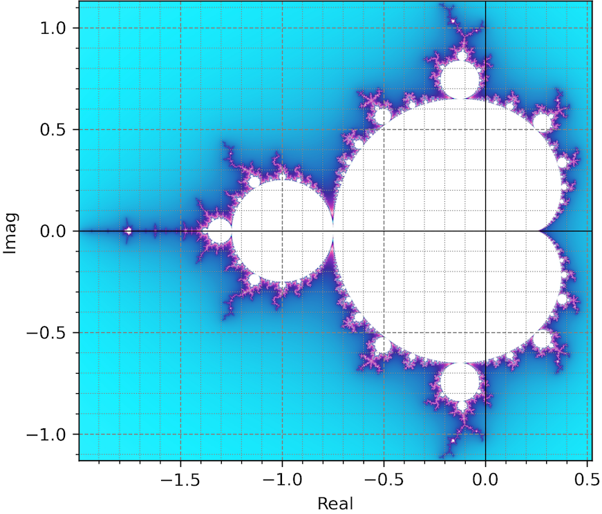
Figure 4: Mandelbrot fractal arising from iterating the square of the propagation vector $C+a^{2}_{\pm}$ shifted for different values of C. The iteration only converges in the white region.

Here the signs $\hat{s}$ and $\tilde{s}$ are only constrained to Eq. (62e) (see Appendix A). Additional relations are:

$$|\hat{a}|^{4}+|\tilde{a}|^{4}=\frac{h^{2}+r^{2}}{2},$$ (63a)

$$a^{2}_{\pm}=r\pm iq=a\pm 2\vv{\rho}\cdot\vv{a_{\pm}}.$$ (63b)

Note that the real and imaginary parts of $a_{\pm}$ define the four eigenvalues of the propagation matrix $\lambda_{1,2,3,4}=\{\,\,\eta_{0}\pm|\hat{a}|\,\,,\,\,\eta_{0}\pm i|\tilde{a}|\,\,\}$, such that they form an equilateral romboid of side $\sqrt{h}$ in the complex plane. This and the above algebraic relationships can be translated into the geometry of Fig. (3). As explained there, the distances between the eigenvalues of $\mathbf{K}$ can be related with the propagation vector and its square, given by $r$ and $q$ in Eq. (61). By choosing a reference system defined by the distance $C=\overline{OO^{\prime}}$ and inclined with respect to the original real axis by an angle $\alpha$, the projections $r$ and $q$ of $a^{2}_{+}$ can be made coincident with $\lambda_{1}$ and be related to the romboid sides. Once the relative size and inclination between r, q, and h has been obtained, we could arbitrarily move and rotate their triangle to a different origin $O^{\prime}$, as shown in the second panel of Fig.(3). Interestingly, as the values of $r$ and $q$ compose the squared complex number $a^{2}_{\pm}$, they form the Mandelbrot fractal (Mandelbrot, 1982) when $(a^{2}_{\pm})_{n+1}=(a^{2}_{\pm})_{n}+C$ is iterated for all values of $C$ in the complex plane (see Fig. 4). We suspect a possible application of the Mandelbrot fractal to understand certain aspects of the Magnus expansion (e.g., its convergence properties, or an eventual relation among its terms, rotations, and the powers of $a_{\pm}$).

4.3 Algebraic characterization of the propagation matrix

In this section, we present the engine of our formalism, a battery of decompositions and calculations that allows to understand the algebra of the propagation matrix and operate conveniently within it.  Semel & López Ariste (1999) and  López Ariste & Semel (1999) investigated the RTE in Stokes formalism and found important to investigate the algebraic structure of the polarized RTE. One of their insights was that the Stokes 4-vector can be seen as an element of a Minkowski-like $\mathbb{R}^{1,3}$ space (with $I$ playing the role of the temporal dimension) with a metric having the norm $\parallel\mathbf{I}\parallel\leq I^{2}-Q^{2}-U^{2}-V^{2}$. Thus, the RTE quantifies all possible infinitesimal transformations between two nearby points lying inside the “Stokes cone of light”. Such transformations are divided in 11 kinds composing a Poincaré group (the inhomogeneous generalization of a Lorentz group) in which dilatations are allowed. The inhomogeneous character is given by the inhomogeneous term in the RTE, i.e. $\bm{\epsilon}$, which quantifies translations along each of the four dimensions. Dilatations appear due to the diagonal of the absorption matrix in Eq. (12):

$$\mathbf{K}(s)=\eta_{0}(s)\mathbbold{1}+\hat{\mathbb{L}}(s),$$ (64)

which reduces/amplifies the number of reemitted photons through indiscriminated positive/negative absorption of photons in any polarization states as of $\rm\eta_{0}=\eta^{(A)}_{0}-\eta^{(S)}_{0}$ is dominated by ordinary absorption ($\eta_{0}^{(A)}$ as in the solar atmosphere, or by stimulated emission ($\eta_{0}^{(S)}$).

The remaining (i.e. the homogeneous) part of the Poincaré group is given by the Lorentz group SO($1,3$), whose elements $\bm{U}$ can be expressed as exponentials of Lorentz matrices $\hat{\mathbb{L}}$, accomplishing (see Section 4.1):

$$\bm{U}^{T}\bm{JU}=\bm{J},$$ (65a)

$$\hat{\mathbb{L}}^{T}\bm{J}+\bm{J}\hat{\mathbb{L}}=0.$$ (65b)

with $\bm{J}=\mathrm{diag}(1,-1,-1,-1)$. The Lorentz matrix $\hat{\mathbb{L}}$ is composed of the 6 infinitesimal generators of rotations of the Lorentz group, i.e. the three $4\times 4$ matrices $\tilde{\mathbf{G}}_{1},\tilde{\mathbf{G}}_{2},\tilde{\mathbf{G}}_{3}$ generating ordinary 3D rotations (anomalous dispersion) in the QUV space, plus the three $4\times 4$ matrices $\hat{\mathbf{G}}_{1},\hat{\mathbf{G}}_{2},\hat{\mathbf{G}}_{3}$ producing hyperbolic rotations (i.e., rotations involving the first dimension) due to dichroism (Lorentz boosts in special relativity theory).

From here, our characterization of the propagation matrix distinguishes four algebraic levels associated to decompositions in: 1) individual Lorentz generators; 2) base matrices; 3) hyperbolic and circular subspaces; and 4) Lorentz matrices. The Lorentz generators in the first level are encoded in $\hat{\mathbb{L}}$ as:

$$\begin{split}&\hat{\mathbf{G}}_{1}^{\leavevmode\hbox to10.36pt{\vbox to10.76pt{\text{[drawing]}}}}+\hat{\mathbf{G}}_{2}^{\leavevmode\hbox to10.93pt{\vbox to10.93pt{\text{[drawing]}}}}+\hat{\mathbf{G}}_{3}^{\leavevmode\hbox to11.78pt{\vbox to12.24pt{\text{[drawing]}}}}+\tilde{\mathbf{G}}_{1}^{\leavevmode\hbox to8.88pt{\vbox to10.19pt{\text{[drawing]}}}}+\tilde{\mathbf{G}}_{2}^{\leavevmode\hbox to9.86pt{\vbox to9.86pt{\text{[drawing]}}}}+\tilde{\mathbf{G}}_{3}^{\leavevmode\hbox to10.19pt{\vbox to8.88pt{\text{[drawing]}}}}=\\ &=\left(\begin{array}[]{cccc}\leavevmode\hbox to16.99pt{\vbox to16.99pt{\text{[drawing]}}}&\leavevmode\hbox to14.63pt{\vbox to15.2pt{\text{[drawing]}}}&\leavevmode\hbox to18.88pt{\vbox to18.88pt{\text{[drawing]}}}&\leavevmode\hbox to14.63pt{\vbox to15.2pt{\text{[drawing]}}}\\ \leavevmode\hbox to14.63pt{\vbox to15.2pt{\text{[drawing]}}}&\leavevmode\hbox to16.99pt{\vbox to16.99pt{\text{[drawing]}}}&\leavevmode\hbox to21pt{\vbox to18.24pt{\text{[drawing]}}}&\leavevmode\hbox to19.22pt{\vbox to19.22pt{\text{[drawing]}}}\\ \leavevmode\hbox to18.88pt{\vbox to18.88pt{\text{[drawing]}}}&\leavevmode\hbox to19.89pt{\vbox to17.28pt{\text{[drawing]}}}&\leavevmode\hbox to16.99pt{\vbox to16.99pt{\text{[drawing]}}}&\leavevmode\hbox to18.24pt{\vbox to21pt{\text{[drawing]}}}\\ \leavevmode\hbox to14.63pt{\vbox to15.2pt{\text{[drawing]}}}&\leavevmode\hbox to20.3pt{\vbox to20.3pt{\text{[drawing]}}}&\leavevmode\hbox to17.28pt{\vbox to19.89pt{\text{[drawing]}}}&\leavevmode\hbox to16.99pt{\vbox to16.99pt{\text{[drawing]}}}\end{array}\right).\end{split} 0 1 1 1 1 0 1 -1 1 -1 0 1 1 1 -1 0 0 1 1 1 1 0 1 -1 1 -1 0 1 1 1 -1 0$$ (66)

Here the geometrical symbols point out the only elements of the corresponding generator matrices that are not zero. They describe rotations in every subspace and they are all orthogonal among them. For all $k$, we find:

$$\mathbf{\hat{G}}_{k}^{2}-\mathbf{\tilde{G}}_{k}^{2} =\mathbbold{1}$$ (67a)

$$\mathbf{\hat{G}}_{k}\cdot\mathbf{\tilde{G}}_{k} =0$$ (67b)

$$\mathbf{\hat{G}}_{k}^{2} =\mathbbold{1}_{k}\quad\Rightarrow\quad\mathbf{\tilde{G}}_{k}^{2}=\mathbbold{1}_{k}-\mathbbold{1},$$ (67c)

where

$$\mathbbold{1}_{k}=\left(\begin{array}[]{cccc}1&0&0&0\\ 0&\delta_{1,k}&0&0\\ 0&0&\delta_{2,k}&0\\ 0&0&0&\delta_{3,k}\\ \end{array}\right).$$ (68)

Equivalently, all the above implies $(\mathbf{\hat{G}}_{k}\pm i\mathbf{\tilde{G}}_{k})^{2}=\mathbbold{1}$. We also introduce a set of dual generators:

$$\begin{split}&\hat{\mathbf{D}}_{1}^{\leavevmode\hbox to10.36pt{\vbox to10.76pt{\text{[drawing]}}}}+\hat{\mathbf{D}}_{2}^{\leavevmode\hbox to10.93pt{\vbox to10.93pt{\text{[drawing]}}}}+\hat{\mathbf{D}}_{3}^{\leavevmode\hbox to11.78pt{\vbox to12.24pt{\text{[drawing]}}}}+\tilde{\mathbf{D}}_{1}^{\leavevmode\hbox to8.88pt{\vbox to10.19pt{\text{[drawing]}}}}+\tilde{\mathbf{D}}_{2}^{\leavevmode\hbox to9.86pt{\vbox to9.86pt{\text{[drawing]}}}}+\tilde{\mathbf{D}}_{3}^{\leavevmode\hbox to10.19pt{\vbox to8.88pt{\text{[drawing]}}}}=\\ &=\left(\begin{array}[]{cccc}\leavevmode\hbox to16.99pt{\vbox to16.99pt{\text{[drawing]}}}&\leavevmode\hbox to14.63pt{\vbox to15.2pt{\text{[drawing]}}}&\leavevmode\hbox to24.43pt{\vbox to24.43pt{\text{[drawing]}}}&\leavevmode\hbox to14.63pt{\vbox to15.2pt{\text{[drawing]}}}\\ \leavevmode\hbox to14.96pt{\vbox to15.2pt{\text{[drawing]}}}&\leavevmode\hbox to16.99pt{\vbox to16.99pt{\text{[drawing]}}}&\leavevmode\hbox to21pt{\vbox to18.24pt{\text{[drawing]}}}&\leavevmode\hbox to21.85pt{\vbox to21.85pt{\text{[drawing]}}}\\ \leavevmode\hbox to18.88pt{\vbox to18.88pt{\text{[drawing]}}}&\leavevmode\hbox to22.61pt{\vbox to19.63pt{\text{[drawing]}}}&\leavevmode\hbox to16.99pt{\vbox to16.99pt{\text{[drawing]}}}&\leavevmode\hbox to18.24pt{\vbox to21pt{\text{[drawing]}}}\\ \leavevmode\hbox to14.96pt{\vbox to15.2pt{\text{[drawing]}}}&\leavevmode\hbox to20.3pt{\vbox to20.3pt{\text{[drawing]}}}&\leavevmode\hbox to19.63pt{\vbox to22.61pt{\text{[drawing]}}}&\leavevmode\hbox to16.99pt{\vbox to16.99pt{\text{[drawing]}}}\end{array}\right).\end{split} 0 1 -1 1 -1 0 1 \,\,1\,\, 1 \,\,1\,\, 0 1 -1 1 \,\,1\,\, 0 0 1 -1 1 -1 0 1 \,\,1\,\, 1 \,\,1\,\, 0 1 -1 1 \,\,1\,\, 0$$ (69)

As before, every dual generator $\mathbf{\hat{D}}_{k}$ or $\mathbf{\tilde{D}}_{k}$ is a $4\times 4$ matrix whose only entries different than zero are those pointed out with the corresponding geometrical symbol. Thus, the anticommutators of the original generators can be neatly expressed as:

$$[\mathbf{\hat{G}}_{i},\mathbf{\hat{G}}_{j}]_{+} =2\cdot\delta_{ij}\mathbbold{1}_{i}+|\epsilon_{ijk}|\mathbf{\tilde{D}}_{k}\quad(\forall i,j)$$ (70a)

$$[\mathbf{\tilde{G}}_{i},\mathbf{\tilde{G}}_{j}]_{+} =2(\mathbbold{1}_{i}-\mathbbold{1})+|\epsilon_{ijk}|\mathbf{\tilde{D}}_{k}\quad(\forall i,j)$$ (70b)

$$[\mathbf{\hat{G}}_{i},\mathbf{\tilde{G}}_{j}]_{+} =\epsilon_{ijk}(-1)^{k}\mathbf{\hat{D}}_{k}\quad(\forall i,j)$$ (70c)

And their ordinary commutators are:

$$[\mathbf{\hat{G}}_{i},\mathbf{\tilde{G}}_{j}] =-\epsilon_{ijk}\mathbf{\hat{G}}_{k}\quad(\forall i,j)$$ (71a)

$$[\mathbf{\hat{G}}_{i},\mathbf{\hat{G}}_{j}] =\epsilon_{ijk}\mathbf{\tilde{G}}_{k}\quad(\forall i,j)$$ (71b)

$$[\mathbf{\tilde{G}}_{i},\mathbf{\tilde{G}}_{j}] =-\epsilon_{ijk}\mathbf{\tilde{G}}_{k}\quad(\forall i,j)$$ (71c)

Instead of infinitesimal generators, sometimes it is more convenient to use denser matrices. Thus, our second algebraic level considers a decomposition in larger subspaces. Namely, we define vectors of hyperbolic and ordinary $4\times 4$ rotation matrices

$$\vv{\mathbf{\hat{G}}} =(\mathbf{\hat{G}}_{1},\mathbf{\hat{G}}_{2},\mathbf{\hat{G}}_{3})$$ (72a)

$$\vv{\mathbf{\tilde{G}}} =(\mathbf{\tilde{G}}_{1},\mathbf{\tilde{G}}_{2},\mathbf{\tilde{G}}_{3}),$$ (72b)

such that any Lorentz matrix $\hat{\mathbb{L}}(s_{i})\equiv\hat{\mathbb{L}}_{i}=\mathbf{H}_{i}+\mathbf{R}_{i}$ at a point $i$ can be neatly decomposed into a hyperbolic rotation $\mathbf{H}_{i}=\vv{\eta}_{i}\cdot\vv{\mathbf{\hat{G}}}$ and an ordinary rotation $\mathbf{R}_{i}=\vv{\rho}_{i}\cdot\vv{\mathbf{\tilde{G}}}$:

$$\hat{\mathbb{L}}_{i}=\left(\begin{array}[]{cccc}0&\eta_{1,i}&\eta_{2,i}&\eta_{3,i}\\ \eta_{1,i}&0&0&0\\ \eta_{2,i}&0&0&0\\ \eta_{3,i}&0&0&0\\ \end{array}\right)+\left(\begin{array}[]{cccc}0&0&0&0\\ 0&0&\rho_{3,i}&-\rho_{2,i}\\ 0&-\rho_{3,i}&0&\rho_{1,i}\\ 0&\rho_{2,i}&-\rho_{1,i}&0\\ \end{array}\right).$$ (73)

Remarkably, any power $n\in\mathbb{Z}$ of $\mathbf{H}$ and $\mathbf{R}$ can be reduced to

$$\mathbf{H}^{2n} =\eta^{2(n-1)}\mathbf{H}^{2}$$ (74a)

$$\mathbf{H}^{2n+1} =\eta^{2n}\mathbf{H}$$ (74b)

$$\mathbf{R}^{2n} =(-1)^{n-1}\rho^{2(n-1)}\mathbf{R}^{2}$$ (74c)

$$\mathbf{R}^{2n+1} =(-1)^{n}\rho^{2n}\mathbf{R},$$ (74d)

which allows to use power series to calculate exactly any function of $\mathbf{H}$ or $\mathbf{R}$ in terms of only $\mathbf{H},\mathbf{R},\mathbf{H}^{2},\mathbf{R}^{2}$, where $\mathbf{H}^{2},\mathbf{R}^{2}$ are easily obtained with

$$\mathbf{H}^{2} =\mathbf{C}(\vv{\eta}),$$ (75a)

$$\mathbf{R}^{2} =\mathbf{C}(\vv{\rho})-\rho^{2}\mathbbold{1},$$ (75b)

and $\mathbf{C}$ is the generic correlation matrix defined as:

$$\mathbf{C}(\vv{u})=\left(\begin{array}[]{cccc}u^{2}&0&0&0\\ 0&u^{2}_{1}&u_{1}u_{2}&u_{1}u_{3}\\ 0&u_{1}u_{2}&u^{2}_{2}&u_{2}u_{3}\\ 0&u_{1}u_{3}&u_{2}u_{3}&u^{2}_{3}\\ \end{array}\right).$$ (76)

For the crossed products, we find interesting that

$$\mathbf{HRH}=\mathbf{RHR}=(\mathbf{HR})^{n}=(\mathbf{RH})^{n}=\mathbf{0}\quad(n\in\mathbb{Z}),$$ (77)

while the basic product $\mathbf{R}\mathbf{H}$ is

$$-\mathbf{Q}^{T}=\mathbf{R}\mathbf{H}=\left(\begin{array}[]{cccc}0&0&0&0\\ (\vv{\eta}\times\vv{\rho})_{1}&0&0&0\\ (\vv{\eta}\times\vv{\rho})_{2}&0&0&0\\ (\vv{\eta}\times\vv{\rho})_{3}&0&0&0\\ \end{array}\right),$$ (78)

for $\mathbf{Q}=\mathbf{H}\mathbf{R}$. Here the oriented surface vector $\vv{S}=\vv{\eta}\times\vv{\rho}$ has as module the area of the paralellogram enclosed by $\vv{\eta}$ and $\vv{\rho}$. Furthermore, $\mathbf{H}$ and $\mathbf{R}$ do not commute:

$$[\mathbf{H}_{i},\mathbf{R}_{j}]=\mathbf{Q}+\mathbf{Q}^{T}=-(\vv{\eta_{i}}\times\vv{\rho_{j}})\cdot\vv{\mathbf{\hat{G}}}\quad\quad(\mathbf{H}-\mathrm{like})$$ (79a)

$$[\mathbf{H}_{i},\mathbf{H}_{j}]=(\vv{\eta_{i}}\times\vv{\eta_{j}})\cdot\vv{\mathbf{\tilde{G}}}\quad\quad(\mathbf{R}-\mathrm{like})$$ (79b)

$$[\mathbf{R}_{i},\mathbf{R}_{j}]=-(\vv{\rho_{i}}\times\vv{\rho_{j}})\cdot\vv{\mathbf{\tilde{G}}}\quad\quad(\mathbf{R}-\mathrm{like}).$$ (79c)

We also obtain nested commutators that are useful to describe the algebra of the Magnus expansion:

$$[\ldots[[\mathbf{H}_{1},\mathbf{R}_{1}],\mathbf{R}_{2}]\ldots,\mathbf{R}_{n}]=$$

$$\,=(-1)^{n}(\ldots((\vv{\eta_{1}}\times\vv{\rho_{1}})\times\vv{\rho_{2}})\times\ldots\times\vv{\rho_{n}})\cdot\vv{\mathbf{\hat{G}}}\quad\,\,(\mathbf{H}-\mathrm{like})$$ (80a)

$$[\ldots[[\mathbf{H}_{0},\mathbf{H}_{1}],\mathbf{H}_{2}]\ldots,\mathbf{H}_{n}]=$$

$$\,=(\ldots((\vv{\eta_{0}}\times\vv{\eta_{1}})\times\vv{\eta_{2}})\times\ldots\times\vv{\eta_{n}})\cdot\vv{\mathbf{\tilde{G}}}\quad\quad(\mathbf{R}-\mathrm{like})$$ (80b)

$$[\ldots[[\mathbf{R}_{0},\mathbf{R}_{1}],\mathbf{R}_{2}]\ldots,\mathbf{R}_{n}]=$$

$$=(-1)^{n}(\ldots((\vv{\rho_{0}}\times\vv{\rho_{1}})\times\vv{\rho_{2}})\times\ldots\times\vv{\rho_{n}})\cdot\vv{\mathbf{\tilde{G}}}\quad\,\,(\mathbf{R}-\mathrm{like})$$ (80c)

Finally, we need the anti-commutator $[\mathbf{H}_{i},\mathbf{R}_{j}]_{+}$. Despite being skew-symmetric in the hyperbolic space, it cannot be neatly expressed in terms of vector of matrices with the generators that we have defined, due to an alterning sign:

$$[\mathbf{H}_{i},\mathbf{R}_{j}]_{+} =\sum_{k}(\vv{\eta}_{i}\times\vv{\rho}_{j})_{k}(-1)^{k}\mathbf{\hat{D}}_{k}=$$ (81a)

$$= \left(\begin{array}[]{cccc}0&-S_{1}&-S_{2}&-S_{3}\\ S_{1}&0&0&0\\ S_{2}&0&0&0\\ S_{3}&0&0&0\\ \end{array}\right).$$ (81f)

The third algebraic level to consider involves a decomposition in basis matrices. When the vector field of any d-dimensional Lie algebra $\mathfrak{g}$ is expressed in terms of basis matrices $\mathbf{B}_{i}$ ($i=1,\ldots,d$), the algebra is characterized by its structure constants $c_{ijk}$:

$$[\mathbf{B}_{i},\mathbf{B}_{j}]=\sum_{k}c_{ijk}\mathbf{B}_{k}\quad(\in\mathfrak{g})$$

We define our basis matrices in terms of generators as:

$$\mathbf{B}_{k} =\hat{\mathbf{G}}_{k}-i\tilde{\mathbf{G}}_{k},\quad\quad(k=1,2,3)$$ (82a)

$$\vv{\mathbf{B}} =(\mathbf{B}_{1},\mathbf{B}_{2},\mathbf{B}_{3}),$$ (82b)

satisfying

$$\mathbf{B}_{i}\mathbf{B}_{j}=\delta_{ij}\mathbbold{1}+i\epsilon_{ijk}\mathbf{B}_{k}=\frac{[\mathbf{B}_{i},\mathbf{B}_{j}]_{+}+[\mathbf{B}_{i},\mathbf{B}_{j}]}{2}\quad(\forall i,j)$$ (83a)

$$\mathbf{B}^{*}_{i}\mathbf{B}^{*}_{j}=\delta_{ij}\mathbbold{1}-i\epsilon_{ijk}\mathbf{B}^{*}_{k}=\frac{[\mathbf{B}^{*}_{i},\mathbf{B}^{*}_{j}]_{+}+[\mathbf{B}^{*}_{i},\mathbf{B}^{*}_{j}]}{2}\quad(\forall i,j)$$ (83b)

$$\mathbf{B}_{k}\cdot\mathbf{B}^{*}_{k}=\mathbbold{1}+2\mathbf{\tilde{G}}^{2}_{k}=2\mathbbold{1}_{k}-\mathbbold{1}\quad(\forall k)$$ (83c)

$$[\mathbf{B}_{i},\mathbf{B}^{*}_{j}]=[\mathbf{B}^{*}_{i},\mathbf{B}_{j}]=0\quad(\forall i,j)$$ (83d)

$$[\mathbf{B}_{i},\mathbf{B}_{j}]=2i\epsilon_{ijk}\mathbf{B}_{k}\quad(\forall i,j)$$ (83e)

$$[\mathbf{B}^{*}_{i},\mathbf{B}^{*}_{j}]=-2i\epsilon_{ijk}\mathbf{B}^{*}_{k}\quad(\forall i,j)$$ (83f)

$$[\mathbf{B}_{i},\mathbf{B}_{j}]_{+}=2\delta_{ij}\mathbbold{1}\quad(\forall i,j)$$ (83g)

$$[\mathbf{B}_{i},\mathbf{B}^{*}_{j}]_{+}=2|\epsilon_{ijk}|\mathbf{\tilde{D}}_{k}+2i\epsilon_{ijk}(-1)^{k}\mathbf{\hat{D}}_{k}\quad(\forall i,j)$$ (83h)

This decomposition leads to a fourth algebraic level involving Lorentz matrices and the propagation vector. Here, we propose the existence of a generalized (complex) Lorentz matrix:

$$\mathbb{L}=\vv{a}\vv{\mathbf{B}}=\hat{\mathbb{L}}+i\tilde{\mathbb{L}}.$$ (84)

Its real part is the ordinary Lorentz matrix $\hat{\mathbb{L}}$ in Eq. (64). However, the imaginary part is a new dual Lorentz matrix containing the same physical information as $\hat{\mathbb{L}}$ but reorganized such that

$$\tilde{\mathbb{L}} =(\vv{\eta}\cdot\vv{\rho})\,\hat{\mathbb{L}}^{-1}$$ (85a)

$$\hat{\mathbb{L}} =\frac{\mathbb{L}+\mathbb{L}^{*}}{2}=\vv{\eta}\cdot\vv{\hat{G}}+\vv{\rho}\cdot\vv{\tilde{G}}$$ (85b)

$$i\,\tilde{\mathbb{L}} =\frac{\mathbb{L}-\mathbb{L}^{*}}{2}=i(\vv{\rho}\cdot\vv{\hat{G}}-\vv{\eta}\cdot\vv{\tilde{G}})$$ (85c)

$$[\mathbb{L},\mathbb{L}^{*}] =[\tilde{\mathbb{L}},\hat{\mathbb{L}}]=0.$$ (85d)

These expressions can be verified with a direct calculation. They show that both Lorentz matrices can be decomposed not only in terms of non-commuting Lorentz generators but also in terms of $\mathbb{L}$ and $\mathbb{L}^{*}$, which always commute in a same spatial point. The inverse of the Lorentz matrix in Eq. (85a) does not exist when the determinant $|\hat{\mathbb{L}}|=0$. The determinant of a matrix is the product of all its eigenvalues, which for $\hat{\mathbb{L}}$ and $\mathbf{K}$ are given by the sets

$$\lambda^{\prime}_{1,2,3,4} =\{\,\,\pm|\hat{a}|\,\,,\,\,\pm i|\tilde{a}|\,\,\}$$ (86a)

$$\lambda_{1,2,3,4} =\{\,\,\eta_{0}\pm|\hat{a}|\,\,,\,\,\eta_{0}\pm i|\tilde{a}|\,\,\},$$ (86b)

containing the components of $a_{\pm}$ (see Eq.61). Multiplying all values in each set, we obtain the determinants:

$$|\hat{\mathbb{L}}| =|\tilde{\mathbb{L}}|=-p^{2}$$ (87a)

$$|\mathbf{K}| =\eta_{0}^{2}[\eta_{0}^{2}-r]+|\hat{\mathbb{L}}|.$$ (87b)

with $p=\vv{\eta}\cdot\vv{\rho}$ and $r=\eta^{2}-\rho^{2}$ (see Eqs. 62). Hence, $\hat{\mathbb{L}}^{-1}$ does not exist when $p=0$, i.e. when $\eta$ or $\rho$ are zero, or when $\vv{\eta}\perp\vv{\rho}$. This omnipresent quantity $p=\vv{\eta}\cdot\vv{\rho}$ is actually determining whether the algebraic systems represented by $\hat{\mathbb{L}}$ and $\hat{\mathbb{L}}^{-1}$ have a unique solution. A null determinant implies eigenvalues with larger degeneracy because one of the matrix rows or columns is not linearly independent, which reduces the dimensionality of the problem (the volumen enclosed by the column vectors collapses along at least one dimension).

Several useful relationships arise from relating the basis and the Lorentz matrices. Considering the normalized vector

$$\vv{u}=\frac{\vv{a}}{a_{+}}=\frac{a_{-}\cdot\vv{a}}{h}=\frac{(\hat{a}-i\tilde{a})\cdot\vv{a}}{h}$$ (88)

it is direct to show that:

$$\vv{u}\vv{B}=\frac{a_{-}\cdot\mathbb{L}}{h}$$ (89a)

$$\vv{u}^{*}\vv{B}^{*}=\frac{a_{+}\cdot\mathbb{L}^{*}}{h}$$ (89b)

$$\frac{\vv{u}\vv{B}+\vv{u}^{*}\vv{B}^{*}}{2}=\frac{\hat{a}\hat{\mathbb{L}}+\tilde{a}\tilde{\mathbb{L}}}{h}$$ (89c)

$$\frac{\vv{u}\vv{B}-\vv{u}^{*}\vv{B}^{*}}{2}=i\frac{\hat{a}\tilde{\mathbb{L}}-\tilde{a}\hat{\mathbb{L}}}{h}$$ (89d)

$$(\vv{u}\vv{B})\cdot(\vv{u}^{*}\vv{B}^{*})=\frac{\mathbb{L}\cdot\mathbb{L}^{*}}{h}.$$ (89e)

And using the commutation rules obtained, we discover that:

$$\mathbb{L}^{2} =a_{+}^{2}\mathbbold{1}\quad;\quad(\mathbb{L^{*}})^{2}=a_{-}^{2}\mathbbold{1}$$ (90a)

$$\hat{\mathbb{L}}^{2}-\tilde{\mathbb{L}}^{2} =r\cdot\mathbbold{1}$$ (90b)

$$\frac{[\tilde{\mathbb{L}},\hat{\mathbb{L}}]_{+}}{2} =\hat{\mathbb{L}}\cdot\tilde{\mathbb{L}}=i\frac{(\mathbb{L}^{2}-(\mathbb{L^{*}})^{2})}{4}=p\cdot\mathbbold{1}$$ (90c)

$$\frac{[\mathbb{L},\mathbb{L}^{*}]_{+}}{2} =\mathbb{L}\cdot\mathbb{L}^{*}=\hat{\mathbb{L}}^{2}+\tilde{\mathbb{L}}^{2}=2\mathbf{K}^{2}-4\eta_{0}\mathbf{K}+(2\eta^{2}_{0}-r)\mathbbold{1}$$ (90d)

To obtain the last equality of Eq.(90d), we made use of Eq. (90b) and of $\hat{\mathbb{L}}^{2}=(\mathbf{K}-\eta_{0}\mathbbold{1})^{2}=\mathbf{K}^{2}-2\eta_{0}\mathbf{K}+\eta^{2}_{0}\mathbbold{1}$.

Using the latter expressions, the powers of $\hat{\mathbb{L}}$ can be recursively calculated as functions of $\hat{\mathbb{L}},\hat{\mathbb{L}}^{2}$, and $\tilde{\mathbb{L}}$:

$$\hat{\mathbb{L}}^{3} =r\hat{\mathbb{L}}+p\tilde{\mathbb{L}}$$ (91a)

$$\hat{\mathbb{L}}^{4} =r\hat{\mathbb{L}}^{2}+p^{2}\mathbbold{1}$$ (91b)

$$\hat{\mathbb{L}}^{5} =(r^{2}+p^{2})\hat{\mathbb{L}}+rp\tilde{\mathbb{L}}$$ (91c)

$$\hat{\mathbb{L}}^{6} =(r^{2}+p^{2})\hat{\mathbb{L}}^{2}+rp^{2}\mathbbold{1}$$ (91d)

$$\hat{\mathbb{L}}^{7} =(r^{2}+2p^{2})r\hat{\mathbb{L}}+(r^{2}+p^{2})p\tilde{\mathbb{L}}$$ (91e)

$$\ldots$$

For $n\geq 2$ and starting from an odd power of the kind $\hat{\mathbb{L}}^{2n-1}=\alpha\hat{\mathbb{L}}+\beta\tilde{\mathbb{L}}$, the rules to obtain the next even and odd powers are:

$$\hat{\mathbb{L}}^{2n} =\alpha\hat{\mathbb{L}}^{2}+p\beta\mathbbold{1}$$ (92a)

$$\hat{\mathbb{L}}^{2n+1} =(r\alpha+p\beta)\hat{\mathbb{L}}+p\alpha\tilde{\mathbb{L}}$$ (92b)

And from previous relations, we obtain:

$$\hat{\mathbb{L}}^{2}+\tilde{\mathbb{L}}^{2} =2\hat{\mathbb{L}}^{2}-r\mathbbold{1}$$ (93a)

$$\hat{\mathbb{L}}^{3}+\tilde{\mathbb{L}}^{3} =(p+r)\hat{\mathbb{L}}+(p-r)\tilde{\mathbb{L}}$$ (93b)

$$\hat{\mathbb{L}}^{4}+\tilde{\mathbb{L}}^{4} =(2p^{2}+r^{2})\mathbbold{1}$$ (93c)

$$\ldots$$

We shall need to have an insight into the specific structure of $\hat{\mathbb{L}}^{2}$ and $\hat{\mathbb{L}}^{3}$. The latter (and any odd power of $\hat{\mathbb{L}}$) can be neatly decomposed by subspaces with $(\mathbf{H}+\mathbf{R})^{3}=\mathbf{H}^{3}+\mathbf{R}^{3}+[\mathbf{H}^{2},\mathbf{R}]_{+}+[\mathbf{R}^{2},\mathbf{H}]_{+}+(\mathbf{H}\mathbf{R}\mathbf{H}+\mathbf{R}\mathbf{H}\mathbf{R})$, which using Eqs. (74a) and (77) gives:

$$\hat{\mathbb{L}}^{3}=[\eta^{2}\vv{\eta}+(\vv{S}\times\vv{\rho})]\cdot\vv{\mathbf{\hat{G}}}-[\rho^{2}\vv{\rho}+(\vv{S}\times\vv{\eta})]\cdot\vv{\mathbf{\tilde{G}}},$$ (94)

For $\hat{\mathbb{L}}^{2}$, we wrote that $\hat{\mathbb{L}}^{2}=\mathbf{K}^{2}-2\eta_{0}\mathbf{K}+\eta^{2}_{0}$. To obtain a more direct expression, using Eqs. (75a) and (81), the structure of $\hat{\mathbb{L}}^{2}$ can be calculated as $(\mathbf{H}+\mathbf{R})^{2}=\mathbf{H}^{2}+\mathbf{R}^{2}+[\mathbf{H},\mathbf{R}]_{+}$:

$$\hat{\mathbb{L}}^{2}=(\mathbf{U}(a)-\rho^{2}\mathbbold{1})+\vv{d}\vv{\mathbf{\tilde{D}}}+\sum_{k}S_{k}(-1)^{k}\mathbf{\hat{D}}_{k},$$ (95)

with $\mathbf{U}(a)=diag\{a^{2},a_{1}^{2},a_{2}^{2},a^{2}_{3}\}$ ($a_{k}$ given in Eq.60a), $d_{k}=\eta_{i}\eta_{j}+\rho_{i}\rho_{j}\,(i\neq j\neq k)$ and $\vv{S}=\vv{\eta}\times\vv{\rho}$. This shows that the structure of $\hat{\mathbb{L}}^{2}$ (and hence of any even power of $\hat{\mathbb{L}}$) cannot be expressed only in terms of $\mathbbold{1}$, $\vv{\mathbf{\hat{D}}}$, and $\vv{\mathbf{\tilde{D}}}$ (due to $\mathbf{U}(a)$ and $(-1)^{k}$).

To obtain a neater expression reflecting the structure of $\hat{\mathbb{L}}^{2}$, we combine Eqs. (93a) and (90d) to see that $\hat{\mathbb{L}}^{2}=\frac{1}{2}(\mathbb{L}\mathbb{L}^{*}+r\mathbbold{1})$. Developing the summations appearing in $\mathbb{L}\cdot\mathbb{L}^{*}$, we reach:

$$\mathbb{L}\cdot\mathbb{L}^{*}=2\sum_{k}|a_{k}|^{2}\mathbbold{1}_{k}-a^{2}\mathbbold{1}+\sum_{k=1,2,3}(g_{k}\mathbf{D}_{k}+g_{k}^{*}\mathbf{D}^{*}_{k}),$$

where $\mathbf{D}_{k}=\mathbf{\tilde{D}}_{k}+i(-1)^{k}\mathbf{\hat{D}}_{k}$ are basis matrices obtained from dual generators and $g_{k}=a_{i}a^{*}_{j}\epsilon_{ijk}$ has coefficients cyclically ordered to give $\epsilon_{ijk}=1$. Writting them as vectors, we finally see that

$$\hat{\mathbb{L}}^{2}=\biggl{(}\mathbf{U}(a)-\rho^{2}\mathbbold{1}\biggr{)}+\Re e\{\vv{g}\cdot\vv{\mathbf{D}}\}.$$ (96)

4.4 Brief characterization of the Jones propagation matrix

Although we shall focus in the Stokes formalism, in this brief section we present a minimal characterization of the propagation matrix in Jones formalism, with the aim of motivating the study of Magnus solutions in it.

We have said that the Jones formalism uses SL$(2,\mathbb{C})$ to represent the four-dimensional rotations associated to the evolution of the polarization. Now the mapping between a point in $\mathbb{R}^{1,3}$ and the matrix vector space is sometimes called spinor map. Then, the correspondence between the Stokes vector emissivity and the Jones emissivity matrix is:

$$\vv{\epsilon}=(\epsilon_{0},\epsilon_{1},\epsilon_{2},\epsilon_{3})\longleftrightarrow\bm{E}=\left(\begin{array}[]{cc}\epsilon_{0}+\epsilon_{1}&\epsilon_{2}-i\epsilon_{3}\\ \epsilon_{2}+i\epsilon_{3}&\epsilon_{0}-\epsilon_{1}\end{array}\right),$$ (97)

where we can separate diagonal and non-diagonal parts using Pauli matrices (Eqs.(55)) and the auxiliar vector $\vv{e}=(\epsilon_{1},\epsilon_{2},\epsilon_{3})$:

$$\bm{E}=\frac{1}{2}[\epsilon_{0}\mathbbold{1}+\vv{e}\vv{\sigma}],$$ (98)

The map between the full propagation vector (associated to Stokes $I,Q,U,V$) and the Jones propagation matrix is:

$$\vv{\alpha}=(\eta_{0},a_{1},a_{2},a_{3})\longleftrightarrow\bm{\breve{K}}=\left(\begin{array}[]{cc}\eta_{0}+a_{1}&a_{2}-ia_{3}\\ a_{2}+ia_{3}&\eta_{0}-a_{1}\end{array}\right),$$ (99)

with $a_{1},a_{2},a_{3}\in\mathbb{C}$. This matrix can also be decomposed as:

$$\bm{\breve{K}} =\frac{1}{2}[\eta_{0}\mathbbold{1}+\vv{a}\cdot\vv{\sigma}]=\frac{1}{2}[\eta_{0}\mathbbold{1}+a_{+}\@vec{X}],\quad\quad\mathrm{with}$$ (100a)

$$\@vec{X} =\frac{1}{a_{+}}\cdot\left(\begin{array}[]{cc}a_{1}&a_{2}-ia_{3}\\ a_{2}+ia_{3}&-a_{1}\end{array}\right)=\vv{u}\cdot\vv{\sigma},$$ (100d)

with normalized propagation vector $\vv{u}=\vv{a}/a_{+}$. Note that $\@vec{X}^{2}=\mathbbold{1}$ and $\@vec{X}=\@vec{X}^{-1}$, which makes the calculation of the powers of $\bm{\breve{K}}$ and its functions a simple task. However, while the Pauli matrices and the Jones emissivity matrix are Hermitian ($\sigma_{k}=\sigma_{k}^{\dagger}$, $\bm{E}=\bm{E}^{\dagger}$), $\@vec{X}$ is not, because the $a_{k}$ components in its complex entries are themselves complex:

$$\@vec{X}^{\dagger}=\frac{1}{a_{-}}\cdot\left(\begin{array}[]{cc}a^{*}_{1}&a^{*}_{2}-ia^{*}_{3}\\ a^{*}_{2}+ia^{*}_{3}&-a^{*}_{1}\end{array}\right)=\vv{u}^{*}\cdot\vv{\sigma}.$$ (101)

The eigenvalues of $\@vec{X}$ and $\bm{\breve{K}}$ are $\lambda^{\prime}_{\pm}=\pm 1$ and $\lambda_{\pm}=(\eta_{0}\pm a_{+})/2$, respectively. This implies the determinant $|\bm{\breve{K}}|=(\eta_{0}^{2}-a^{2}_{+})/4$.

In the spirit of what we did in the analysis of the Stokes propagation matrix, we can calculate several quantities that appear when operating with the Jones propagation matrix. Calling $z:=\vv{a}a_{-}=\hat{z}+i\tilde{z}$, we define and calculate:

$$\@vec{\hat{Y}}:=\frac{\@vec{X}+\@vec{X}^{\dagger}}{2}=\frac{\hat{z}}{h}\vv{\sigma}$$ (102a)

$$\@vec{\tilde{Y}}:=\frac{\@vec{X}-\@vec{X}^{\dagger}}{2}=\frac{\tilde{z}}{h}\vv{\sigma}$$ (102b)

$$\@vec{\tilde{Y}}\cdot\@vec{\hat{Y}}=\frac{[\@vec{X},\@vec{X}^{\dagger}]}{4}=-\frac{(\vv{\eta}\times\vv{\rho})\cdot\vv{\sigma}}{h}$$ (102c)

$$(a_{+}\@vec{X})\cdot(a_{-}\@vec{X}^{\dagger})=a\cdot\mathbbold{1}-2(\vv{\eta}\times\vv{\rho})\cdot\vv{\sigma}$$ (102d)

$$\@vec{\hat{X}}:=\frac{a_{+}\@vec{X}+a_{-}\@vec{X}^{\dagger}}{2}=\left(\begin{array}[]{cc}\eta_{Q}&\eta_{U}-i\eta_{V}\\ \eta_{U}+i\eta_{V}&-\eta_{Q}\end{array}\right)=\vv{\eta}\cdot\vv{\sigma}$$ (102g)

$$\@vec{\tilde{X}}:=\frac{a_{+}\@vec{X}-a_{-}\@vec{X}^{\dagger}}{2}=i\left(\begin{array}[]{cc}\rho_{Q}&\rho_{U}-i\rho_{V}\\ \rho_{U}+i\rho_{V}&-\rho_{Q}\end{array}\right)=i\vv{\rho}\cdot\vv{\sigma}$$ (102j)

$$\@vec{\hat{X}}\cdot(-i\@vec{\tilde{X}})=(\vv{\eta}\cdot\vv{\sigma})(\vv{\rho}\cdot\vv{\sigma})=(\vv{\eta}\cdot\vv{\rho})\mathbbold{1}-i(\vv{\eta}\times\vv{\rho})\cdot\vv{\sigma}.$$ (102k)

The vector products can be substituted by commutators with:

$$-(\vv{\eta}\times\vv{\rho})\cdot\vv{\sigma}=\frac{i}{2}[\vv{\eta}\cdot\vv{\sigma},\vv{\rho}\cdot\vv{\sigma}]=\frac{[\@vec{\hat{X}},\@vec{\tilde{X}}]}{2}.$$ (103)

Such vector products give a vector perpendicular to the plane defined by $\vv{\eta}$ and $\vv{\rho}$, and its mutiplication by $\vv{\sigma}$ gives a matrix describing three-dimensional rotations around such a normal vector (see Section 4.1). The above quantities are simpler and more compact than their counterparts in Stokes formalism. They also gives a better insight because are easy to interpret in terms of rotors and base Pauli matrices. Furthermore, the simple decomposition in Eq. (100) allows to obtain the corresponding Magnus evolution operator in Jones formalism by just applying Eq. (45)(BE theorem) with $\vv{u}$ the normalized propagation vector. Comparing with the Stokes formalism, the only step that could parallel its complexity in the Jones formalism seems to be the inhomogeneous solution in Eq. (17), which involves a double multiplication by the evolution operator. These reasons justify our interest in using the Magnus expansion to reformulate the radiative transfer problem also in Jones formalism, as we do in the following sections for the Stokes formalism.

5 Reformulation of the homogeneous solution in the Lorentz group (Stokes formalism)

5.1 Derivation of the evolution operator for non-constant $\mathbf{K}$

We can finally derive an analytical evolution operator that allows for arbitrary variations of $\mathbf{K}$. We start truncating the Magnus expansion in Eq. (41) to retain its first term. The algebraic analysis performed in Section (4.3) allows to calculate it explicitly in more than one way. Our approach begins decomposing $\mathbf{K}(s)$ in terms of generalized Lorentz matrices with Eqs. (64) and (85b):

$$\mathbf{K}(s)=\eta_{0}(s)\mathbbold{1}+\frac{\mathbb{L}(s)+\mathbb{L}^{*}(s)}{2}.$$ (104)

The commutation among $\mathbb{L}$ and $\mathbb{L}^{*}$ allows to divide the Magnus evolution operator in three exponentials:

$$\begin{split}\rm{\mathbf{O}}(s)=&e^{-\int^{s}_{s_{0}}dt\mathbf{K}(t)}=\\ =&e^{-\int^{s}_{s_{0}}dt\eta_{0}(t)}\cdot e^{-\frac{1}{2}\int^{s}_{s_{0}}dt\vv{a}(t)\vv{\mathbf{B}}}\cdot e^{-\frac{1}{2}\int^{s}_{s_{0}}dt\vv{a}^{*}(t)\vv{\mathbf{B}}^{*}}\end{split}$$ (105)

This step is not obvious because the exponents contain integrals combining all points along the ray, so let us be more specific. Calling $\vv{b}=\int^{s}_{s_{0}}dt\vv{a}(t)$, the two latter exponents are matrices that can be written together as

$$\begin{split}-\frac{1}{2}[\vv{\mathbf{B}}\vv{b}+\vv{\mathbf{B}}^{*}\vv{b}^{*}]\end{split}$$

because $\vv{\mathbf{B}}$ is a vector of basis (hence constant) matrices. To divide in two exponentials, any component of $\vv{\mathbf{B}}\vv{b}$ must commute with any other of $\vv{\mathbf{B}}^{*}\vv{b}^{*}$, which occurs due to Eq. (83d) because

$$\begin{split}[\mathbf{B}_{i}b_{i},\mathbf{B}^{*}_{j}b^{*}_{j}]&=(b_{i}\mathbf{B}_{i})(b^{*}_{j}\mathbf{B}^{*}_{j})-(b^{*}_{j}\mathbf{B}^{*}_{j})(b_{i}\mathbf{B}_{i})=\\ &=b_{i}b^{*}_{j}\mathbf{B}_{i}\mathbf{B}^{*}_{j}-b_{i}b^{*}_{j}\mathbf{B}^{*}_{j}\mathbf{B}_{i}=b_{i}b^{*}_{j}[\mathbf{B}_{i},\mathbf{B}^{*}_{j}]=0,\end{split}$$ (106)

Then, we can apply the BE theorem (Sec. 3.4) to each matrix exponential in Eq. (105), obtaining

$$\begin{split}\rm{\mathbf{O}}(s)=e^{-\eta^{\prime}_{0}}\cdot[ch(b)\mathbbold{1}-sh(b)\vv{u}\vv{\mathbf{B}}]\cdot[ch(b^{*})\mathbbold{1}-sh(b^{*})\vv{u}^{*}\vv{\mathbf{B}}^{*}],\end{split}$$ (107)

with $b$ and $\vv{u}$ casting $a_{+}$ and $\vv{a}/a_{+}$ in Sec. 4.2, but built from integrated coefficients $\eta^{\prime}_{k}$ ($k=0,1,2,3$) and $\rho^{\prime}_{k}$ ($k=1,2,3$):

$$\vv{u}=\frac{\vv{b}}{b}=\frac{(b_{1},b_{2},b_{3})}{[b^{2}_{1}+b^{2}_{2}+b^{2}_{3}]^{1/2}}=\frac{(\hat{b}-i\tilde{b})}{h}(b_{1},b_{2},b_{3})$$ (108a)

$$b_{k}(s)=\int^{s}_{s_{0}}a_{k}(t)dt=\int^{s}_{s_{0}}\eta_{k}(t)dt+i\int^{s}_{s_{0}}\rho_{k}(t)dt=\eta^{\prime}_{k}+i\rho^{\prime}_{k}$$ (108b)

$$\hat{b}^{2}=(h+r)/2$$ (108c)

$$\tilde{b}^{2}=(h-r)/2$$ (108d)

$$h=[r^{2}+q^{2}]^{1/2}\quad(=\hat{b}^{2}+\tilde{b}^{2})$$ (108e)

$$r=(\vv{\eta}^{\prime})^{2}-(\vv{\rho}^{\prime})^{2}\quad(=\hat{b}^{2}-\tilde{b}^{2})$$ (108f)

$$q=2(\vv{\eta}^{\prime}\cdot\vv{\rho}^{\prime})\quad(=2\hat{b}\tilde{b})$$ (108g)

This move allows to express everything in terms of the seven basic integrals $b_{k}$ as elementary coefficients. Next, we perform the products in Eq. (107), identify matrix terms with Eqs. (89), and apply Appendix C to separate the real ($\hat{b}$) and imaginary ($\tilde{b}$) parts of $b$ and $b^{*}$. This leads to:

$$\begin{split}\mathbf{O}(s)=e^{-\eta^{\prime}_{0}}\cdot\Bigl{\{}c_{0}\mathbbold{1}-\frac{1}{h}\left[c_{1}\hat{\mathbb{L}}+c_{2}\tilde{\mathbb{L}}+c_{3}(\hat{\mathbb{L}}^{2}+\tilde{\mathbb{L}}^{2})\right]\Bigr{\}},\end{split}$$ (109)

with

$$c_{0,3} =\frac{\mathrm{ch}(2\hat{b})\pm\cos(2\tilde{b})}{2}$$

$$c_{1,2} =\frac{\mathrm{sh}(2\hat{b})\mp i\sin(2\tilde{b})}{2}.$$ (110a)

Finally, substituting Eq. (93) for $\hat{\mathbb{L}}^{2}+\tilde{\mathbb{L}}^{2}$ and operating, we find

$$\begin{split}\mathbf{O}(s)=e^{-\eta^{\prime}_{0}}\cdot\Bigl{\{}f_{0}\mathbbold{1}+f_{1a}\hat{\mathbb{L}}+f_{1b}\tilde{\mathbb{L}}+f_{2}\hat{\mathbb{L}}^{2}\Bigr{\}},\end{split}$$ (111)

with scalar functions

$$\begin{split}f_{0}&=\frac{\tilde{b}^{2}\mathrm{ch}(2\hat{b})+\hat{b}^{2}\cos(2\tilde{b})}{\hat{b}^{2}+\tilde{b}^{2}}\quad;f_{1a}=-\left[\frac{\hat{b}\,\mathrm{sh}(2\hat{b})+\tilde{b}\sin(2\tilde{b})}{\hat{b}^{2}+\tilde{b}^{2}}\right]\\ f_{2}&=\frac{\mathrm{ch}(2\hat{b})-\cos(2\tilde{b})}{\hat{b}^{2}+\tilde{b}^{2}}\quad\quad\quad;f_{1b}=\frac{\hat{b}\sin(2\tilde{b})-\tilde{b}\,\mathrm{sh}(2\hat{b})}{\hat{b}^{2}+\tilde{b}^{2}}.\end{split}$$ (112)

Alternative expressions for the evolution operator can be obtained using Eqs. (91) to remove the $\tilde{\mathbb{L}}$ in Eq.(111), writting it as function of any odd power of $\hat{\mathbb{L}}$. For instance, substituting it in terms of $\hat{\mathbb{L}}$ and $\hat{\mathbb{L}}^{3}$ with Eq. (91a), we obtain:

$$\begin{split}\mathbf{O}(s)=e^{-\eta^{\prime}_{0}}\cdot\Bigl{\{}f_{0}\mathbbold{1}+f_{1}\hat{\mathbb{L}}+f_{2}\hat{\mathbb{L}}^{2}+f_{3}\hat{\mathbb{L}}^{3}\Bigr{\}},\end{split}$$ (113)

where the new functions are just

$$\begin{split}f_{1}&=-\left[\frac{\tilde{b}^{2}\,\mathrm{sh}(2\hat{b})+\hat{b}^{2}\sin(2\tilde{b})}{\hat{b}^{2}+\tilde{b}^{2}}\right]\\ f_{3}&=-\left[\frac{\mathrm{sh}(2\hat{b})}{\hat{b}}+\frac{\sin(2\tilde{b})}{\tilde{b}}.\right]\end{split}$$ (114)

The two expressions for the evolution operator can be simplified further by identifying subspaces of constant infinitesimal generators($\vv{\mathbf{\hat{G}}}$, $\vv{\mathbf{\tilde{G}}}$), which allows a convenient integration of the evolution operator in the next sections. Namely, dividing the matrices in Eq. (111) in subspaces, operating, and regrouping, we find the remarkable expression:

$$\begin{split}\mathbf{O}(s)=e^{-\eta^{\prime}_{0}}\cdot\Bigl{\{}\mathbf{\mathring{K}}+f_{2}\hat{\mathbb{L}}^{2}\Bigr{\}},\end{split}$$ (115)

whose new matrix $\mathbf{\mathring{K}}=f_{0}\mathbbold{1}+\vv{\hat{\alpha}}\cdot\vv{\mathbf{\hat{G}}}+\vv{\tilde{\alpha}}\cdot\vv{\mathbf{\tilde{G}}}$ has same structure as $\mathbf{K}$ but with a new propagation vector

$$\begin{split}\vv{\alpha}&=\vv{\hat{\alpha}}+i\vv{\tilde{\alpha}}=-[\mathrm{sh}(2\hat{b})+i\sin(2\tilde{b})]\vv{u},\end{split}$$ (116)

being $\vv{u}$ still given by Eq.(108) and $\hat{\mathbb{L}}^{2}$ by Eq.(95).

Our three expressions for the evolution operator, Eqs. (111), (113), and (115), are fully equivalent. They all are more general and significantly simpler than the one given by LD85. They are general because they preserve memory of the spatial variations (of any arbitrary $\mathbf{K}$) encoded as ray path integrals of optical coefficients, as defined in Eq.(108b). They express everything in terms of the seven basic scalar integrals in $b_{k}$, which seems to be the minimal and most efficient integration possible to solve the RTE for non-constant properties. Thus, by separating the integration from the algebraic calculation of the evolution operator, we expect to obtain more general and efficient numerical solutions for the RTE.

We remark that the Lorentz matrices in our expressions also contain those integrated coefficients (although the matrices are still called as in previous sections). Indeed, the relative simplicity of our expressions comes from writing them in terms of the (integrated) Lorentz matrix $\hat{\mathbb{L}}=\mathbf{K}^{\prime}(s)-\eta^{\prime}_{0}(s)\mathbbold{1}=\vv{\eta}^{\prime}\cdot\vv{\hat{G}}+\vv{\rho}^{\prime}\cdot\vv{\tilde{G}}$. This is also true for the dual Lorentz matrix $\tilde{\mathbb{L}}$ in Eq. (111) because it has the same algebraic structure as $\hat{\mathbb{L}}$. Namely, recalling Eqs.(85), $\tilde{\mathbb{L}}$ is not only proportional to $\hat{\mathbb{L}}^{-1}$ but also $\tilde{\mathbb{L}}=\vv{\rho}^{\prime}\cdot\vv{\hat{G}}-\vv{\eta}^{\prime}\cdot\vv{\tilde{G}}$, hence both $\tilde{\mathbb{L}}$ and $\hat{\mathbb{L}}$ are effortlessly built from each other by exchanging $\eta^{\prime}_{k}\leftrightarrow\rho^{\prime}_{k}$ and $\rho^{\prime}_{k}\leftrightarrow-\eta^{\prime}_{k}$.

Considering also that we know the specific elements of $\hat{\mathbb{L}}^{2}$ by Eq.(95), or that it can be cheaply calculated multiplying $\hat{\mathbb{L}}$ by itself, we see that our solution for the exponential evolution operator is optimal. In essence, it is just a matter of adding up two composed matrices ($\hat{\mathbb{L}}^{2}$ and $\mathbf{\mathring{K}}$), half of them containing redundant information (due to their symmetries). Hence, our calculation of the matrix exponential is not only analytical, but also seems ideal for numerical applications, because involves the minimal number of operations to solve exactly an evolution operator accounting for arbitrary spatial variations of $\mathbf{K}$.

Our evolution operator in Eq. (115) reveals other insight: $\hat{\mathbb{L}}^{2}$ is the only term whose algebra differs from that of $\mathbf{K}$ in the homogeneous solution, making explicit that $\hat{\mathbb{L}}^{2}$ is the only algebraic difference between the Lorentz group (where the evolution operator belongs) and its Lie algebra, where $\mathbf{K}$ belongs. To verify that our result belongs to the Lorentz group, one could use Eq. (51). Particularizing our expressions to the case of constant propagation matrix, one recovers the result of LD85.

5.2 Higher order terms of the Magnus expansion

The BE theorem allows to calculate the exponential of the Magnus expansion including only its first order term $\mathbf{\Omega}_{1}$. Here we give a preliminar exploration of our Magnus solution when $\mathbf{\Omega}_{2}$ is included. Decomposing with Eqs. (85b) and (85d), the $\mathbf{\Omega}_{2}$ for the RTE becomes:

$$\mathbf{\Omega}_{2}(s)=-\frac{1}{2}\int^{s}_{s_{0}}d_{1}\int^{s_{1}}_{s_{0}}d_{2}\biggl{[}\,\mathbf{K}(s_{1})\mathbf{K}(s_{2})-\mathbf{K}(s_{2})\mathbf{K}(s_{1})\biggr{]}=$$ (117a)

$$= -\frac{1}{2}\int^{s}_{s_{0}}d_{1}\int^{s_{1}}_{s_{0}}d_{2}\biggl{[}\mathbb{\hat{L}}(s_{1}),\mathbb{\hat{L}}(s_{2})\biggr{]}.$$ (117b)

The latter commutator can be worked out with the relation

$$[\vv{\mathrm{v}_{1}}\cdot\vv{\mathbf{B}},\vv{\mathrm{v}_{2}}\cdot\vv{\mathbf{B}}]=2i(\vv{\mathrm{v}_{1}}\times\vv{\mathrm{v}_{2}})\cdot\vv{\mathbf{B}},$$ (118)

being $\vv{\mathbf{B}}$ our vector of basis matrices. Thus, we obtain (calling generically $X_{i}$ to $X(s_{i})$)

$$\begin{split}&[\mathbb{\hat{L}}_{1},\mathbb{\hat{L}}_{2}]=\frac{i}{2}\biggl{[}(\vv{a}_{1}\times\vv{a}_{2})\vv{\mathbf{B}}-(\vv{a}^{*}_{1}\times\vv{a}^{*}_{2})\vv{\mathbf{B}^{*}}\biggr{]}=\Re e\Biggl{\{}\frac{i}{2}\vv{a}_{1x2}\cdot\vv{\mathbf{B}}\Biggr{\}}=\\ &=\biggl{[}(\vv{\eta}_{1}\times\vv{\eta}_{2})-(\vv{\rho}_{1}\times\vv{\rho}_{2})\biggr{]}\vv{\mathbf{\tilde{G}}}-\biggl{[}(\vv{\eta}_{1}\times\vv{\rho}_{2})+(\vv{\rho}_{1}\times\vv{\eta}_{2})\biggr{]}\vv{\mathbf{\hat{G}}},\end{split}$$ (119)

with $\vv{a}_{1x2}=\vv{a}(s_{1})\times\vv{a}(s_{2})$. Then,

$$\begin{split}\mathbf{\Omega}_{2}(s)=&\biggl{[}\,\int^{s}_{s_{0}}ds_{1}\frac{(\vv{\eta}_{1}\times\vv{\rho}^{\prime}_{1})+(\vv{\rho}_{1}\times\vv{\eta}^{\prime}_{1})}{2}\biggr{]}\vv{\mathbf{\hat{G}}}\,+\\ +&\biggl{[}\,\int^{s}_{s_{0}}ds_{1}\frac{(\vv{\rho}_{1}\times\vv{\rho}^{\prime}_{1})-(\vv{\eta}_{1}\times\vv{\eta}^{\prime}_{1})}{2}\biggr{]}\vv{\mathbf{\tilde{G}}}.\end{split}$$ (120)

with

$$\vv{\eta}^{\prime}_{1} =\vv{\eta}^{\prime}(s_{1})=\int^{s_{1}}_{s_{0}}ds_{2}\vv{\eta}(s_{2})$$ (121a)

$$\vv{\rho}^{\prime}_{1} =\vv{\rho}^{\prime}(s_{1})=\int^{s_{1}}_{s_{0}}ds_{2}\vv{\rho}(s_{2}).$$ (121b)

Comparison of this result with the different decompositions of the Lorentz matrix (Section 4.3) shows explicitly that the matrix structure of $\mathbf{\Omega}_{2}$ is that of the Lorentz matrix, as expected in this Lie algebra. As the same is true for all terms of the Magnus expansion, their addition to $\mathbf{\Omega}_{1}$ will give an exponential evolution operator of the same form as Eq.(115), but with $f_{0}$, $f_{2}$ and $\vv{\alpha}$ increasingly complicated by the presence of nested integrals of nested vector products, in a similar fashion to Eq. (120). It is a matter of ongoing numerical investigation to find out how to calculate such integrals efficiently to avoid significant penalty when extending our methods to higher orders of the expansion.

6 Reformulation of the inhomogeneous problem with Magnus in Stokes formalism

The general evolution operator derived analytically in the previous section can be directly inserted into Eq. (23) to obtain a new family of numerical methods based on the Magnus expansion. Such methods would already represent a fundamental improvement to solve the RTE. However, there are certain issues that motivate an alternative formulation of the inhomogeneous problem too. The inhomogeneous RTE:

$$\begin{split}\mathbf{I}^{\prime}(s)&=\mathbf{A}(s)\mathbf{I}(s)+{\bm{\epsilon}}(s)\quad\quad;\mathbf{I}(0)=\mathbf{I}_{0}\end{split}$$ (122)

with $\mathbf{A}(s)=-\mathbf{K}(s)$ can be solved with Eq. (23). In the most general case, the evolution operators in it are substituted by the full Magnus exponential. In this paper we shall start considering Eq. (123) as a result of truncating the Magnus expansion to first order, in consistency with our previous section, and yet allowing for variations of the $\mathbf{K}(s)$ matrix in $\mathbf{A}(s)$. Then:

$$\begin{split}\mathbf{I}(s)&=e^{\int^{s}_{0}\mathbf{A}(\tau)d\tau}\mathbf{I}_{0}+\int^{s}_{0}e^{\int^{s}_{t}\mathbf{A}(\tau)d\tau}{\bm{\epsilon}}(t)\,dt.\end{split}$$ (123)

Once we study and test our methods for this case, we will study higher orders. The problem here is that the calculation of the inhomogeneous integral with the nested integral in the inner exponent is costly and of difficult evaluation because we need two different sets of quadrature points for nested integrals changing in different intervals. To solve this problem, we reformulate it.

6.1 Reformulating the case with constant properties

For $\mathbf{A}$ constant, the typical formal inhomogeneous solution given by Eq.(23) can be considered local because is restricted to small regions/cells of constant properties. As we anticipated, it is also inconsistent and innacurate, because it breaks the inhomogeneous group structure when $\mathbf{A}$ is constant but ${\bm{\epsilon}}$ is not. In order to introduce our method of solution for the general case, we first consider the simplest consistent system, given by Eq. (123) with both $\mathbf{A}$ and ${\bm{\epsilon}}$ constant. Its solution can be written in terms of a matrix function ${\bm{\phi}}_{1}(s\mathbf{A})$, both as

$$\mathbf{I}(s)=e^{s\mathbf{A}}\mathbf{I}_{0}+\int^{s}_{0}e^{(s-t)\mathbf{A}}{\bm{\epsilon}}\,dt=e^{s\mathbf{A}}\mathbf{I}_{0}+s{\bm{\phi}}_{1}(s\mathbf{A}){\bm{\epsilon}}$$ (124)

or as

$$\begin{split}&\mathbf{I}(s)=e^{s\mathbf{A}}\mathbf{I}_{0}+(e^{s\mathbf{A}}-\mathbbold{1})\mathbf{A}^{-1}{\bm{\epsilon}}=e^{s\mathbf{A}}(\mathbf{I}_{0}+\mathbf{A}^{-1}\mathbf{\epsilon})-\mathbf{A}^{-1}{\bm{\epsilon}}=\\ &=\mathbf{I}_{0}+s{\bm{\phi}}_{1}(s\mathbf{A})(\mathbf{A}\mathbf{I}_{0}+{\bm{\epsilon}}),\end{split}$$ (125)

where we define ${\bm{\phi}}_{1}(s\mathbf{A})$ in several ways:

$${\bm{\phi}}_{1}(s\mathbf{A}) =\frac{1}{s}\int^{s}_{0}e^{(s-t)\mathbf{A}}\,dt=\frac{1}{s}\int^{s}_{0}e^{t\mathbf{A}}\,dt=$$ (126a)

$$=\sum^{\infty}_{n=0}\frac{(s\mathbf{A})^{n}}{(n+1)!}=$$ (126b)

$$=(e^{s\mathbf{A}}-\mathbbold{1})(s\mathbf{A})^{-1}=\quad\biggl{(}\equiv\frac{e^{x}-\mathbbold{1}}{x}\biggr{)}$$ (126c)

$$=\int^{1}_{0}e^{zs\mathbf{A}}\,dz.$$ (126d)

Eq. (126a) shows the relation of ${\bm{\phi}}_{1}(s\mathbf{A})$ with Eq. (125), while Eq. (126b) shows its relation with the exponential

$$\begin{split}e^{s\mathbf{A}}&=\sum^{\infty}_{n=0}\frac{(s\mathbf{A})^{n}}{n!}.\\ \end{split}$$ (127)

Alternatively, Eq. (126c) gives an inefficient way of calculating ${\bm{\phi}}_{1}(s\mathbf{A})$, while Eq. (126d) gives an efficient integral definition in terms of a parameter $z$.

Our method of solution is based on the realization that the Eq. (123) with both $\mathbf{A}$ and ${\bm{\epsilon}}$ constant is equivalent to a $5\times 5$ homogeneous system

$$\begin{split}\frac{d}{ds}\left(\begin{array}[]{c}\mathbf{I}(s)\\ I_{t}\end{array}\right)&=\left(\begin{array}[]{cc}\mathbf{A}&{\bm{\epsilon}}\\ \mathbf{0}^{\intercal}&0\end{array}\right)\left(\begin{array}[]{c}\mathbf{I}(s)\\ I_{t}\end{array}\right)\end{split}$$ (128)

with $\mathbf{I}(0)=\mathbf{I}_{0},I_{t}(0)=1$, $I_{t}$ a mere auxiliar value, and whose new $5\times 5$ propagation matrix $\mathcal{A}_{5}$ contains $\mathbf{A}\equiv\mathbf{A}_{4\times 4}$. Correspondingly, the solution in Eq. (124) can be seen to be equivalent to (see also Eq. (26))

$$\mathbf{I}_{5}(s)=e^{s\mathcal{A}_{5}}\mathbf{I}_{5,0}=\left(\begin{array}[]{cc}e^{s\mathbf{A}}&s{\bm{\phi}}_{1}(s\mathbf{A}){\bm{\epsilon}}\\ \mathbf{0}^{\intercal}&0\end{array}\right)\mathbf{I}_{5,0}$$ (129)

with $\mathbf{I}_{5,0}=\mathbf{I}_{5}(0)=(\mathbf{I}_{0},1)^{\intercal}$. Eq. (129) tells us that the inhomogeneous solution for $\mathcal{A}_{5}$ constant can be written as a ${5\times 5}$ evolution operator containing both the corresponding ${4\times 4}$ evolution operator and a special product involving ${\bm{\phi}}_{1}$. Let us now apply this to the general case.

6.2 Reformulating the general case with variable properties

The method that we propose consists in extending by one the dimension of the inhomogeneous problem to convert it in a five-dimensional homogeneous one, and thus solve it with the Magnus expansion. Namely, Eq. (123) is equivalent to a $5\times 5$ homogeneous system

$$\begin{split}\frac{d}{ds}\left(\begin{array}[]{c}\mathbf{I}(s)\\ I_{t}\end{array}\right)&=\left(\begin{array}[]{cc}\mathbf{A}(s)&{\bm{\epsilon}}(s)\\ \mathbf{0}^{T}&0\end{array}\right)\left(\begin{array}[]{c}\mathbf{I}(s)\\ I_{t}\end{array}\right)\end{split}$$ (130)

with $\mathbf{I}_{5,0}=\mathbf{I}_{5}(0)=(\mathbf{I}_{0},1)^{\intercal}$, and where again we call $\mathbf{I}_{5}$(s) to the solution vector of unknowns and $\mathcal{A}_{5}$(s) to the new propagation matrix containing the original $\mathbf{A}(s)=-\mathbf{K}(s)$. Being homogeneous, this system can be solved applying the Magnus expansion to $\mathcal{A}_{5}(s)$. We do this considering only $\mathbf{\Omega}_{1}$ in the Magnus expansion, to keep consistency with the evolution operator that we derived in the previous section. Thus, we have to calculate:

$$\begin{split}\rm{\mathbf{O}}_{5}(s)=&e^{\int^{s}_{s_{0}}\mathcal{A}_{5}(t)dt}=e^{\bar{\mathcal{A}}_{5}}=\sum^{\infty}_{n=0}\frac{\bar{\mathcal{A}}_{5}^{n}}{n!}.\end{split}$$ (131)

where the overbars mean integration hereafter:

$$\bar{\mathcal{A}}_{5} =\left(\begin{array}[]{cc}\bar{\mathbf{A}}&\bar{{\bm{\epsilon}}}\\ \mathbf{0}^{\intercal}&0\end{array}\right)$$ (132c)

$$\bar{\mathbf{A}} =-\int^{s}_{s_{0}}\mathbf{K}(t)dt$$ (132d)

$$\bar{{\bm{\epsilon}}} =\int^{s}_{s_{0}}{\bm{\epsilon}}(t)dt=(\epsilon^{\prime}_{0},\epsilon^{\prime}_{1},\epsilon^{\prime}_{2},\epsilon^{\prime}_{3})^{\intercal}$$ (132e)

The integral of $\mathbf{K}$ contains the seven ray-path scalar integrals of Eq.(108), $\eta^{\prime}_{k}(k=0,1,2,3)$ and $\rho^{\prime}_{k}(k=1,2,3)$, while $\bar{\bm{\epsilon}}$ contains the four equivalent scalar integrals $\epsilon^{\prime}_{k}(k=0,1,2,3)$.

As the powers of $\bar{\mathcal{A}}_{5}$ show the simple general form

$$\begin{split}\bar{\mathcal{A}}_{5}^{n}&=\left(\begin{array}[]{cc}\bar{\mathbf{A}}^{n}&\bar{\mathbf{A}}^{n-1}\bar{{\bm{\epsilon}}}\\ \mathbf{0}^{\intercal}&0\end{array}\right),\end{split}$$ (133)

all terms in Eq. (131) can be readily resummed to obtain

$$\rm{\mathbf{O}}_{5}(s) =\left(\begin{array}[]{cc}e^{\bar{\mathbf{A}}}&\Biggl{[}\sum^{\infty}_{n=0}\frac{\bar{\mathbf{A}}^{n}}{(n+1)!}\Biggr{]}\bar{{\bm{\epsilon}}}\\ \mathbf{0}^{\intercal}&1\end{array}\right)=\left(\begin{array}[]{cc}e^{\bar{\mathbf{A}}}&{\bm{\phi}}_{1}(\bar{\mathbf{A}})\bar{{\bm{\epsilon}}}\\ \mathbf{0}^{\intercal}&1\end{array}\right)$$ (134e)

$$=\mathbbold{1}_{5}+\left(\begin{array}[]{cc}{\bm{\phi}}_{1}(\bar{\mathbf{A}})\bar{\mathbf{A}}&{\bm{\phi}}_{1}(\bar{\mathbf{A}})\bar{{\bm{\epsilon}}}\\ \mathbf{0}^{\intercal}&0\end{array}\right),$$ (134h)

Inserting these two equivalent expressions into the general solution $\mathbf{I}_{5}(s)=\rm{\mathbf{O}}_{5}(s)\mathbf{I}_{5,0}$, and taking the $4\times 4$ subspace, we find:

$$\mathbf{I}(s) =e^{\bar{\mathbf{A}}}\mathbf{I}_{0}+{\bm{\phi}}_{1}(\bar{\mathbf{A}})\bar{{\bm{\epsilon}}}=$$ (135a)

$$=\mathbf{I}_{0}+{\bm{\phi}}_{1}(\bar{\mathbf{A}})(\bar{\mathbf{A}}\mathbf{I}_{0}+\bar{{\bm{\epsilon}}}),$$ (135b)

which reduces to Eqs. (124) and (125) when both $\mathbf{A}$ $(i.e.,-\mathbf{K})$ and ${\bm{\epsilon}}$ are constant.

What has just happened in Eqs. (135)? The inhomogeneous formal integral that has always characterized the solution to the radiative transfer problem and its numerical methods has vanished. Eq. (135) substitutes it by the product of an integrated emissivity vector and a special function of an integrated propagation matrix. We can explain this saying that, by solving the $4\times 4$ inhomogeneous problem as the Magnus solution to a $5\times 5$ homogeneous problem, we are solving the translations given by the emissivity term in the Poincaré space of the solution as if they were rotations quantified by the new algebra of the $5\times 5$ Magnus expansion. Thus, Eq. (135) gives a radically different way of solving the radiative transfer problem (see next subsection 6.4).

Let us also comment on Eq. (134e), which shows that the algebra of the 5D propagation matrix is such that the 4D subspace containing the homogeneous solution (i.e. the evolution operator) is always independent on the inhomogeneous part of the system containing the special function ${\bm{\phi}}_{1}$ and the emissivity. This implies that if we extend the Magnus expansion to higher orders, we can always continue using the corresponding evolution operator because the only thing that changes is how the function ${\bm{\phi}}_{1}$ is combined with the emisivity. For instance, if we add $\mathbf{\Omega}_{2}$ to the Magnus expansion we would be adding a term of the kind of Eq.(120), with the commutator :

$$\begin{split}[\mathcal{A}_{5}(s_{1}),&\mathcal{A}_{5}(s_{2})]=\mathcal{A}_{5}(s_{1})\mathcal{A}_{5}(s_{2})-\mathcal{A}_{5}(s_{2}),\mathcal{A}_{5}(s_{1})=\\ &=\left(\begin{array}[]{cc}[\mathbf{A}(s_{1}),\mathbf{A}(s_{2})]&\mathbf{A}(s_{1}){\bm{\epsilon}}(s_{2})-\mathbf{A}(s_{2}){\bm{\epsilon}}(s_{1})\\ \mathbf{0}^{\intercal}&0\end{array}\right).\end{split}$$ (136)

This shows that the $4\times 4$ subspace is preserved, containing a commutator similar to that with $\mathcal{A}_{5}$. Thus, after integrating and exponentiating, the new solution will have the new evolution operator (now including $\Omega_{2}$) and a composition of matrix-vector products between ${\bm{\phi}}_{1}$ and integrals of $\mathbf{A}$ and ${\bm{\epsilon}}$. We will have to find the right balance between more general theoretical description (higher order in Magnus) and more efficient computational representation (higher numerical order of integration and fastest calculation).

6.3 Calculation of ${\bm{\phi}}_{1}$: integrating the evolution operator

Taking now Eq. (135a) as an efficient general expression, we make it fully explicit by calculating ${\bm{\phi}}_{1}(\bar{\mathbf{A}})={\bm{\phi}}_{1}(-\bar{\mathbf{K}})$. Namely, integrating along a parameter $z$ with Eq. (126d)

$${\bm{\phi}}_{1}(-\bar{\mathbf{K}})=\int^{1}_{0}e^{z\bar{\mathbf{A}}(s)}\,dz=\int^{1}_{0}e^{-\int^{s}_{s_{0}}z\mathbf{K}(t)dt}\,dz=\int^{1}_{0}O(t,z)\,dz,$$ (137)

we see that ${\bm{\phi}}_{1}(-\bar{\mathbf{K}})$ is obtained integrating our evolution operator in Eq. (115) after assigning the parameter $z$ to every matrix component of $\mathbf{K}$, i.e. to every integrated optical coefficient $\eta^{\prime}$ and $\rho^{\prime}$ in Eqs. (108c). Guided by Eq. (107), and propagating $z$ to all the subsequent quantities, we see that the only place where the propagated parameter $z$ does not cancel out is inside the trigonometrical expressions, because any other quantity depending on $\eta^{\prime}$ and $\rho^{\prime}$ (i. e. the normalized vector $\vv{u}$, and $b_{k}$, $\hat{b}$, or $\tilde{b}$) has a denominator that always cancels out the $z$ dependence. We make this clear by specifying all the subspaces in Eq. (115) for the evolution operator and adding the parameter z where it remains:

$$\begin{split}\mathbf{O}(s,z)&=e^{-\eta^{\prime}_{0}z}\cdot\Biggl{\{}\frac{\tilde{b}^{2}\mathrm{ch}(2\hat{b}z)+\hat{b}^{2}\cos(2\tilde{b}z)}{\hat{b}^{2}+\tilde{b}^{2}}\mathbbold{1}+\\ &-\Re e\Bigl{\{}[\mathrm{sh}(2\hat{b}z)+i\sin(2\tilde{b}z)]\vv{u}\Bigr{\}}\cdot\vv{\mathbf{\hat{G}}}\,+\\ &-\Im m\Bigl{\{}[\mathrm{sh}(2\hat{b}z)+i\sin(2\tilde{b}z)]\vv{u}\Bigr{\}}\cdot\vv{\mathbf{\tilde{G}}}\,+\\ &+\frac{\mathrm{ch}(2\hat{b}z)-\cos(2\tilde{b}z)}{\hat{b}^{2}+\tilde{b}^{2}}\biggl{(}\mathbf{U}(a)-\rho^{2}\mathbbold{1}+\Re e\{\vv{g}\cdot\vv{\mathbf{D}}\}\biggr{)}\Biggr{\}},\end{split}$$ (138)

with $\mathbf{U}(a)=diag\{a^{2},a_{1}^{2},a_{2}^{2},a^{2}_{3}\}$, $g_{k}=a_{i}a^{*}_{j}\epsilon_{ijk}$, and $a_{k}$ given in Eq.(60a). Hence, the only integrals that appear are

$$\int^{1}_{0}e^{-\eta^{\prime}_{0}z}\mathrm{ch}(2\hat{b}z)dz =\frac{e^{-\eta^{\prime}_{0}}[-\eta^{\prime}_{0}\mathrm{ch}(2\hat{b})-2\hat{b}\,\mathrm{sh}(2\hat{b})]+\eta^{\prime}_{0}}{{\eta^{\prime}_{0}}^{2}-(2\hat{b})^{2}}$$ (139a)

$$\int^{1}_{0}e^{-\eta^{\prime}_{0}z}\cos(2\tilde{b}z)dz =\frac{e^{-\eta^{\prime}_{0}}[-\eta^{\prime}_{0}\cos(2\tilde{b})+2\tilde{b}\sin(2\tilde{b})]+\eta^{\prime}_{0}}{{\eta^{\prime}_{0}}^{2}+(2\tilde{b})^{2}}$$ (139b)

$$\int^{1}_{0}e^{-\eta^{\prime}_{0}z}\mathrm{sh}(2\hat{b}z)dz =\frac{e^{-\eta^{\prime}_{0}}[-\eta^{\prime}_{0}\,\mathrm{sh}(2\hat{b})-2\hat{b}\,\mathrm{ch}(2\hat{b})]+2\hat{b}}{{\eta^{\prime}_{0}}^{2}-(2\hat{b})^{2}}$$ (139c)

$$\int^{1}_{0}e^{-\eta^{\prime}_{0}z}\sin(2\tilde{b}z)dz =\frac{e^{-\eta^{\prime}_{0}}[-\eta^{\prime}_{0}\sin(2\tilde{b})-2\tilde{b}\cos(2\tilde{b})]+2\tilde{b}}{{\eta^{\prime}_{0}}^{2}+(2\tilde{b})^{2}}$$ (139d)

Once substituted the integrals and the vector $\vv{u}$ (see Eq.108a):

$$\vv{u}=\frac{\vv{b}}{b}=\frac{(\hat{b}-i\tilde{b})}{h}(\vv{\eta^{\prime}}+i\vv{\rho^{\prime}}),$$ (140)

we rearrange and identify terms. First, we arrange things to identify the trigonometric functions:

$$\hat{c} =\frac{\mathrm{ch}(2\hat{b})}{\eta^{\prime}_{0}\hat{d}}\quad;\quad\tilde{c}=\frac{\cos(2\tilde{b})}{\eta^{\prime}_{0}\tilde{d}}$$ (141a)

$$\hat{s} =\frac{\mathrm{sh}(2\hat{b})}{2\hat{b}\hat{d}}\quad;\quad\tilde{s}=\frac{\sin(2\tilde{b})}{2\tilde{b}\tilde{d}},$$ (141b)

containing well-behaving sync functions

$$\lim_{\hat{b}\to 0}\frac{\mathrm{sh}(2\hat{b})}{2\hat{b}}=\lim_{\tilde{b}\to 0}\frac{\sin(2\tilde{b})}{2\tilde{b}}=1$$ (142)

and

$$\begin{split}\hat{d}&={\eta^{\prime}_{0}}^{2}-(2\hat{b})^{2}\quad;\quad\tilde{d}={\eta^{\prime}_{0}}^{2}+(2\tilde{b})^{2}.\end{split}$$ (143)

Recombining subspaces for $\vv{\mathbf{\hat{G}}}$ and $\vv{\mathbf{\tilde{G}}}$, and keeping terms in $\mathbbold{1}$ and $\hat{\mathbb{L}}^{2}$, we identify the Lorentz matrices $\hat{\mathbb{L}}$, $\tilde{\mathbb{L}}$ and $\hat{\mathbb{L}}^{2}$. Thus, after a cumbersome calculation, we obtain:

$$\begin{split}{\bm{\phi}}_{1}(-\bar{\mathbf{K}})&={\bm{\phi}}_{A}+{\bm{\phi}}_{B}=\\ &=\frac{{\eta^{\prime}_{0}}^{2}e^{-\eta^{\prime}_{0}}}{\hat{b}^{2}+\tilde{b}^{2}}\cdot\Biggl{\{}n_{1}\mathbbold{1}+n_{2}\hat{\mathbb{L}}+n_{3}\tilde{\mathbb{L}}+n_{4}\hat{\mathbb{L}}^{2}\Biggr{\}}+\\ &+\frac{4\eta^{\prime}_{0}}{\hat{d}\tilde{d}}\cdot\Biggl{\{}\biggl{(}\frac{\eta^{\prime}_{0}}{2}-r\biggr{)}\mathbbold{1}-\frac{\eta^{\prime}_{0}}{2}\hat{\mathbb{L}}+n_{r}\tilde{\mathbb{L}}+\hat{\mathbb{L}}^{2}\Biggr{\}},\end{split}$$ (144)

with $n_{r}=\frac{2\hat{b}\tilde{b}}{\eta^{\prime}_{0}}$ and

$$n_{1} =(\tilde{b}^{2}\hat{c}+\hat{b}^{2}\tilde{c})+n_{r}^{2}(\hat{s}-\tilde{s})$$ (145a)

$$n_{2} =\frac{2}{\eta^{\prime}_{0}}\Bigl{[}(\hat{s}+\hat{c})\hat{b}^{2}+(\tilde{s}+\tilde{c})\tilde{b}^{2}\Bigr{]}$$ (145b)

$$n_{3} =n_{r}\Bigl{[}(\hat{s}+\hat{c})-(\tilde{s}+\tilde{c})\Bigr{]}$$ (145c)

$$n_{4} =4(\hat{b}^{2}\hat{s}+\tilde{b}^{2}\tilde{s})-(\hat{c}-\tilde{c})$$ (145d)

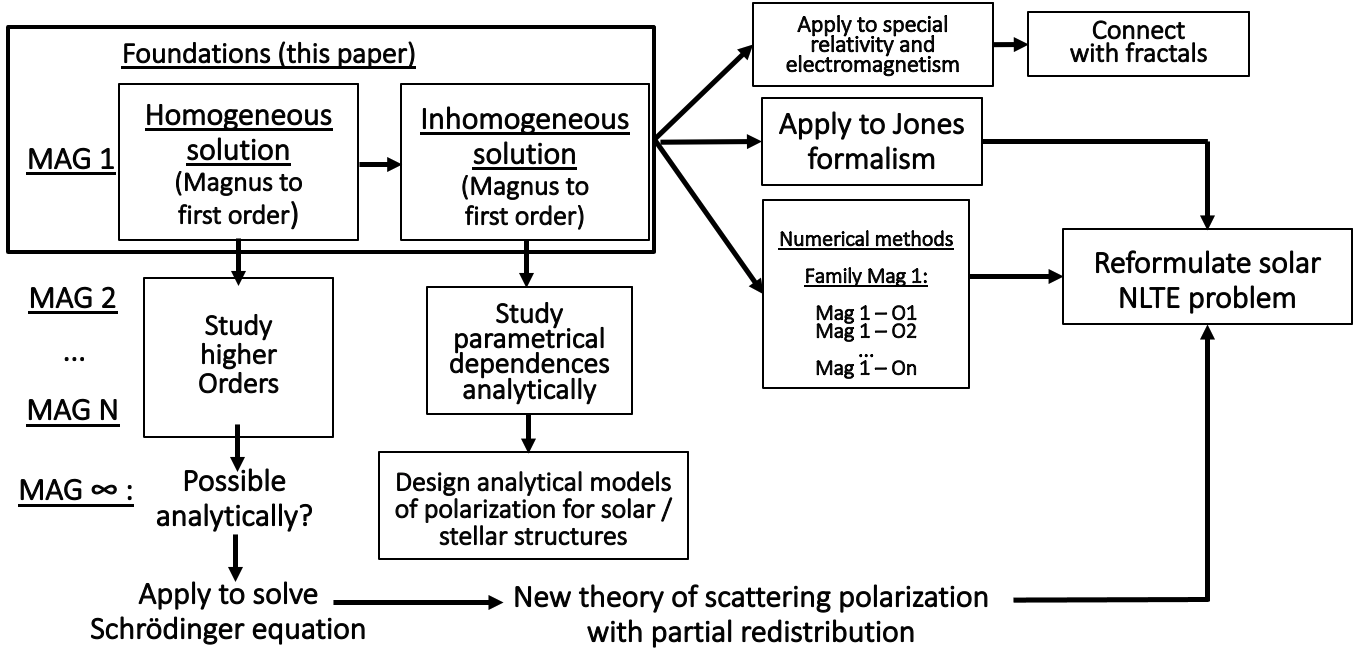
Figure 5: Research prospects.

For the sake of clarity, we have divided Eq. (144) into two matrices ${\bm{\phi}}_{A}$ and ${\bm{\phi}}_{B}$, showing different external dependence on $\eta^{\prime}_{0}$, but both belonging to the Lorent group. I.e., their algebraic structure match that of the evolution operator, thus depending on the same basic Lorentz matrices that were already built from integrated optical coefficients, but multiplied by simple scalar functions. With this explicit analytical calculation, the computational cost of building our formal solution in Eq. (135a), which furthermore only contains two matrix-vector products, should be minimal. Note also that, once the order of the Magnus expansion is set, our whole development of the evolution operator and of the inhomogeneous solution with ${\bm{\phi}}_{1}$ has been mathematically exact.

6.4 Additional comments and prospects

In summary, we have reformulated the radiative transfer problem to obtain consistent integral solutions based on the Magnus expansion. Starting by truncating the expansion to first order, we have arrived to Eq. (135)

$$\begin{split}\mathbf{I}(s)&=e^{-\bar{\mathbf{K}}}\mathbf{I}_{0}+{\bm{\phi}}_{1}(-\bar{\mathbf{K}})\bar{{\bm{\epsilon}}},\\ \end{split}$$

with the exponential evolution operator given explicitly by Eq. (115), ${\bm{\phi}}_{1}(-\bar{\mathbf{K}})$ given by Eq. (144), and $\bar{\mathbf{K}}$ and $\bar{{\bm{\epsilon}}}$ containing the eleven basic scalar ray-path integrals of the optical coefficients. By having an exact analytical formula for both a consistent inhomogeneous solution and an evolution operator considering arbitrary variations of $\mathbf{K}$, we now can (see Fig. 5):

• 1) Find consistent solutions respecting the Lie group structure at any step of the calculations, thus solving accurately the exact physical problem, instead of a similar one. The obvious prospect here is to extend our formulation to include higher order terms of the Magnus expansion.

• 2) Define a new family of numerical methods implementing Eq. (135a). These methods should be advantageous from the start, simply because they are based on a more accurate, compact, and efficient representation of the physical and mathematical problem. However, one of the numerical aspects that should be investigated is how non-local is our theory for the order of the Magnus expansion considered. A key to investigate this is the convergence of the Magnus expansion, which could set a limiting range that depends on our specific application. Our research and numerical developments are ongoing and will be available to the astrophysical community when ready.

• 3) Understand polarized radiative transfer in depth. As our formal solution is analytical and non-local (not restricted to relatively small regions or cells of constant properties), the general long-range solution to the RTE can be studied theoretically as a function of its parameters, thus transcending previous approximate radiative transfer models. For instance, now it would be possible to explain without strong approximations the joint action of magneto-optical and dichroic effects in certain wavelengths of the polarization profiles, something that could only be done independently for every mechanism (as made for dichroism in Carlin, 2019).

• 4) Incorporate a defined geometry in the radiative transfer problem analytically, thus building analytical models of complex astrophysical objects (e.g., a whole star) that can however be taylored to the physical information available. Thus, we can study the physics of these objects with polarization fingerprints transparently, without radiative transfer itself being a source of error. This is possible because the main input for our equations, the eleven ray-path scalar integrals of the optical coefficients, cannot only be provided by realistic atmosphere models but also by exact prescribed functional variations of the atmosphere.

• 5) Reformulate the methods of solution for the NLTE problem with polarization to make them non-local. This novel idea seems very interesting. By considering variations of $\mathbf{K}$, both our evolution operator and the final inhomogeneous solution are non-markovian in space, i.e. they preserve memory of the atmospheric physics in previous locations along the ray. This memory can be used, at least in principle, to accelerate the NLTE interation between the RTE and the rate equations in the theory of scattering polarization. Of interest here is that our theory separates the integration of the optical coefficients from the algebraic construction of the formal solution, which permits to compute the latter only once directly at the end of the ray (or at any intermediate location), and reduces the numerical task to the simplest integration possible, i.e. to the scalar integration of the eleven basic optical coefficients of the problem.

• 6) Solve general physical problems with a similar algebraic structure to that of the RTE. With small cosmetic changes (reinterpreting the physical quantities), our equations also give novel solutions for other homogeneous and inhomogeneous problems of universal interest that share the Lorentz/Poincaré group structure, again allowing arbitrary variations of their system matrix. Well-known examples are the motion of masses at relativistic speeds, and the calculation of Lorentz forces on charged particles moving in an electromagnetic field.

7 Conclusions

We have laid the foundations to solve the polarized radiative transfer problem in a new, efficient, and fully consistent way using the Magnus expansion. First, we presented a succint rederivation of the radiative tranfer equations (RTE) in Stokes and Jones formalisms using a common nomenclature and consistent physical conventions for the phase of the electric field and the signs of Stokes V. We believe that now the equations of both formalism can be used and compared on a more clear basis.

Truncating the Magnus expansion to first order, and applying our BE theorem (Sec. 3.4), we have obtained three equivalent analytical expressions of a new and more general evolution operator that allows for arbitrary spatial variations of the propagation matrix (Sec. 5.1). Our Basic Evolution theorem calculates analytically the exact exponential of any integral of the propagation matrix, illustrating the possibility of introducing the scalar integrals of the optical coefficients inside the terms of our solutions. This ends up being equivalent to separate the integration from the composition of the formal solution. Furthermore, it allows to calculate the solution at the end of a ray without necessarily doing matrix calculations or solving the formal solution at every intermediate point. Developing the order two of the Magnus expansion, we have shown some prospects for generalizing the evolution operator to higher orders of the expansion.

As an insight, we interpret the evolution of the solution to the RTE as complex multidimensional rotations in the Lie algebra of the Lorentz/Poincaré group. Such rotations are quantified by rotors whose direction and strength of rotation are given by the normalized propagation vector. As shown by the compact formulation of our evolution operator, such a rotational evolution is neatly expressed at the level of the Lie group with a linear combination of our generalized Lorentz matrix and the square of the ordinary Lorentz matrix (the only factor in the solution that does not belong to the Lie algebra). Here we remark that our calculations were made easier by our algebraic characterization of the propagation matrix, including its generators, powers, commutators, and the different ways in which we can decompose it to operate (Sec. 4.3).

Finally, by increasing the dimensionality of the $4\times 4$ problem to $5\times 5$, we have reformulated the inhomogeneous solution as an homogeneous one, which is again solved with the Magnus expansion to first order. Thus, the typical formal integral of previous formulations is substituted by an integral function of our evolution operator. Calculating it analytically and exactly, we arrive to an explicit radiative transfer solution whose inputs are the simple ray-path scalar integrals of the eleven optical coefficient of the radiative transfer problem.

For several reasons, our approach is potentially disruptive for solar spectropolarimetry. First of all, it is the first one that fully solves the RTE consistently, explicitly, and allowing for arbitrary ray-path variations of the propagation matrix. Secondly, it poses the integration of the RTE in a radically new way. Instead of integrating an standard formal solution to solve the inhomogeneous problem many times along every ray, our theory is built in such a way that in principle allows to integrate directly and exactly the scalar optical coefficients of the problem for the whole ray and, only then, substitute the result in an analytical expression with minimal algebraic complexity.

Furthermore, by including a Magnus evolution operator and a Magnus inhomogeneous solution, our results natively preserves the full Lie group structure of the problem. On one hand, this means that the evolution of the solution follows its correct geometrical space in the algebra. In other words, we should now be able to integrate over large distances along the ray with a significantly smaller departure from the right solution. On the other hand, in principle we could use our new evolution operator to calculate more general response functions in the NLTE problem. These two key aspects suggests a reformulation of the NLTE problem with polarization that could allow to solve this non-local problem in a non-local way for the first time. This is critical for accelarating inversions of Stokes profiles, on which solar diagnosis is based. Besides, our preliminar calculations (Sec. 4.4) suggests to investigate whether is advantageous to reformulate our Magnus-based solutions in Jones formalism, whose algebra involves simpler $2\times 2$ matrices. In that case, a reformulation of the NLTE problem in Jones formalism could be advisable.

Using the Magnus expansion, our formulation allows to naturally generalize our evolution operator for higher orders of accuracy even before considering to increase the numerical order, something that previous methods were unable to do. We speculate that if the new terms of such generalization could be ideally resummed into tractable scalar functions, we could be opening the door to solve the radiative transfer problem in the most general, efficient, and exact way possible.

Given the algebraic similarity with other physical universal problems with Lorentz/Poincaré algebra, our results are applicable to them after a mere reinterpretation of the physical quantities.

Appendix A Calculation of real and imaginary parts of the propagation module

If $\vv{a}=\vv{\eta}+i\vv{\rho}=(\eta_{1}+i\rho_{1},\eta_{2}+i\rho_{2},\eta_{3}+i\rho_{3})$, the modules of $\vv{a}(\equiv\vv{a}_{+})$ and $\vv{a}^{*}(\equiv\vv{a}_{-})$ are complex numbers that we call $a_{+}$ and $a_{-}$, respectively. To calculate them we state:

$$a_{\pm} =\hat{a}\pm i\tilde{a}\quad\quad(\hat{a},\tilde{a}\in\mathbb{R}),$$

$$a^{2}_{\pm} =\vv{\eta}^{2}-\vv{\rho}^{2}\pm i2\vv{\eta}\cdot\vv{\rho}=\hat{a}^{2}-\tilde{a}^{2}\pm i2\hat{a}\tilde{a}$$

where we identify the real numbers

$$r =\vv{\eta}^{2}-\vv{\rho}^{2}=\hat{a}^{2}-\tilde{a}^{2}$$

$$q =2\vv{\eta}\cdot\vv{\rho}=2\hat{a}\tilde{a},$$

$$h =[r^{2}+q^{2}]^{1/2}=a_{-}\cdot a_{+}=\hat{a}^{2}+\tilde{a}^{2}$$

Substituting $\hat{a}=q/(2\tilde{a})$ in $r=\hat{a}^{2}-\tilde{a}^{2}$ we obtain $4\tilde{a}^{4}+4r\tilde{a}^{2}-q^{2}=0$ and find the solutions:

$$\hat{a}=\pm\left(\frac{\pm h+r}{2}\right)^{1/2},\quad\tilde{a} =\pm\left(\frac{\pm h-r}{2}\right)^{1/2}.$$

The signs acompanying $h$ must be chosen positive for $\hat{a}$, $\tilde{a}\in\mathbb{R}$. Regarding the outer signs of the roots, one is tempted to choose the sign of $\hat{a}$ positive because $\hat{a}$ works as an attenuation factor. Landi Deglinnocenti & Landi Deglinnocenti (1985) solved a similar problem to this before us, imposing positive sign for a proportional quantity equivalent to our $\hat{a}$ (which they called $\alpha$). However such imposition is unnecesary to solve the above equations and would be wrong in a general case in which stimulated emission could dominate. Note that the total absorption coefficient $\eta_{0}\pm|\hat{a}|>0$, appearing e.g. in the eigenvalues of the propagation matrix or in the expressions of the evolution operator, is always positive with $\eta_{0}>0$ and $|\hat{a}|<\eta_{0}$ when stimulated emission does not dominate. We then avoid to impose the outer signs, labelling them as $\hat{s}$ and $\tilde{s}$:

$$\hat{a}=\hat{s}\left(\frac{h+r}{2}\right)^{1/2},\quad\quad\tilde{a} =\tilde{s}\left(\frac{h-r}{2}\right)^{1/2}.$$

The signs are however constrained by the angle $\theta$ between $\vv{\eta}$ and $\vv{\rho}$ in the QUV space, because $\hat{s}\cdot\tilde{s}=sign(\hat{a}\cdot\tilde{a})=sign(\vv{\eta}\cdot\vv{\rho})=sign(\cos\theta)$. Thus, when $\vv{\eta}\perp\vv{\rho}$ the signs are undetermined, but then the expressions involucrating them will become independent on them.

Appendix B Proof of the Basic Evolution theorem

The evolution theorem gives the solution to the exponential of the integral of an arbitrary matrix $N$. To demonstrate the theorem, we start decomposing the matrix as $\mathbf{N}=f\,\vv{n}\cdot\vv{\sigma}$, with $f$ an arbitrary constant, $\vv{n}=(n_{1},\ldots,n_{d})$ a vector of components, and $\vv{\mathbf{\sigma}}=(\mathbf{\sigma}_{1},\ldots,\mathbf{\sigma}_{d})$ a vector of basis matrices with algebra $\mathfrak{g}$ that must fulfill:

$$\mathbf{\sigma}_{k}\cdot\sigma_{\ell}=\delta_{k{\ell}}\mathbbold{1}+h\cdot\epsilon_{k{\ell}m}\cdot\sigma_{m},\quad\quad(h=ct.)$$ (150)

This condition implies both $\sigma^{2}_{k}=\mathbbold{1}$ and vanishing anticommutators $[\sigma_{k},\sigma_{\ell}]_{+}=\sigma_{k}\sigma_{\ell}+\sigma_{\ell}\sigma_{k}=0$ for all $k\neq{\ell}$. The following step is now to calculate the generic integral of $N$:

$$\mathcal{I}=\int ds\,\mathbf{N}(s)=\int ds\,f\,\vv{n}(s)\cdot\vv{\sigma}=f\sum^{d}_{k=1}b_{k}\sigma_{k}=f\,\vv{b}\cdot\vv{\sigma}$$ (151a)

where we defined the integrated vector $\vv{b}=(b_{1},\ldots,b_{d})$, having module $b$ and components:

$$b_{k}=\int n_{k}(s)ds$$ (152)

Condition (150) simplify calculation of $\mathcal{I}^{2}$ as:

$$\frac{\mathcal{I}^{2}}{f^{2}}=\left(\sum^{d}_{k=1}b_{k}\sigma_{k}\right)^{2}=\sum_{k={\ell}}b^{2}_{k}\sigma^{2}_{k}+\sum_{k\neq{\ell}}b_{k}b_{\ell}[\sigma_{k},\sigma_{\ell}]_{+}=b^{2}\mathbbold{1}$$ (153a)

Hence, the even and odd powers of the integral are $\mathcal{I}^{2k}=(fb)^{2k}\mathbbold{1}$ and $\mathcal{I}^{2k+1}=\mathcal{I}^{2k}\cdot\mathcal{I}=(fb)^{2k+1}\vv{u}\cdot\vv{\sigma}$, in terms of the unitary vector

$$\vv{u}=\frac{\vv{b}}{b}.$$ (154)

Thus, the exponential of $\mathcal{I}$ can be finally calculated as:

$$e^{\pm\int ds\,\mathbf{N}(s)}= \sum^{\infty}_{k=0}\frac{(\pm\mathcal{I})^{k}}{k!}=\sum^{\infty}_{k=0}\frac{\mathcal{I}^{2k}}{(2k)!}\pm\sum^{\infty}_{k=0}\frac{\mathcal{I}^{2k+1}}{(2k+1)!}=$$

$$= \sum^{\infty}_{k=0}\frac{(fb)^{2k}}{(2k)!}\mathbbold{1}\pm\sum^{\infty}_{k=0}\frac{(fb)^{2k+1}}{(2k+1)!}\vv{u}\cdot\vv{\sigma}=$$

$$= \,\mathrm{ch}(fb)\mathbbold{1}\pm\mathrm{sh}(fb)\mathbf{U},$$ (155a)

where the matrix $\mathbf{U}=\vv{u}\cdot\vv{\sigma}$, and $b$ and $\vv{u}$ are given by Eqs. (152) and (154).

Appendix C Trigonometrical expressions for the coefficients of the analytical EO

The following four coefficients with complex argument $x=\hat{x}+i\tilde{x}$ are developed to find several equivalent convenient expressions:

$$c_{0}=\cosh(x)\cosh(x^{*}) =\cosh^{2}(\hat{x})+\sinh^{2}(i\tilde{x})=$$

$$=\cosh^{2}(\hat{x})-\sin^{2}(\tilde{x})=$$

$$=\frac{\cosh(2\hat{x})+\cos(2\tilde{x})}{2}$$

$$c_{1}=\cosh(x)\sinh(x^{*}) =\frac{\sinh(2\hat{x})-i\sin(2\tilde{x})}{2}$$

$$c_{2}=\cosh(x^{*})\sinh(x) =\frac{\sinh(2\hat{x})+i\sin(2\tilde{x})}{2}$$

$$c_{3}=\sinh(x)\sinh(x^{*}) =\cosh^{2}(\hat{x})-\cosh^{2}(i\tilde{x})=$$

$$=\cosh^{2}(\hat{x})-\cos^{2}(\tilde{x})$$

$$=\frac{\cosh(2\hat{x})-\cos(2\tilde{x})}{2}.$$ (156a)

As trigonometrical expressions for double angle miminimizes numerical error for small arguments, we choose:

$$c_{0,3} =\frac{\cosh(2\hat{x})\pm\cos(2\tilde{x})}{2}$$

$$c_{1,2} =\frac{\sinh(2\hat{x})\mp i\sin(2\tilde{x})}{2}.$$ (157a)