Asymptotic bound on slow-roll parameter in stringy quintessence model

Min-Seok Seo^a

^aDepartment of Physics Education, Korea National University of Education,
Cheongju 28173, Republic of Korea

We study the late time behavior of the scalar part of the volume modulus and the dilaton in stringy quintessence model, focusing on their contributions to the Hubble slow-roll parameter $\epsilon$ which directly measures the deviation of the spacetime geometry from de Sitter space. When only one of the moduli is allowed to move, $\epsilon$ converges to the stable fixed point at late time. The fixed point value is larger than $1$, thus the slow-roll cannot be realized. Moreover, if the decay rate of the quintessence potential is larger than some critical value, the positivity of the potential imposes that the stable fixed point value is just given by $3$, independent of the details of the moduli dynamics. Otherwise, the fixed point value coincides with the potential slow-roll parameter. When both the volume modulus and the dilaton roll down the potential simultaneously, we can find the relation between the contributions of two moduli to $\epsilon$ satisfied at the fixed point. In this case, the fixed point value is not in general the simple sum of fixed point values in the single field case and cannot be larger than $3$.

1 Introduction

Construction of the model for the universe compatible with the cosmological observations [2] has been one of challenges in string phenomenology. In particular, whereas models like the KKLT [3] or the large volume scenario [4] have been proposed to realize the metastable de Sitter (dS) vacuum which well describes the observed almost constant vacuum energy density, the suspicion has been raised that some unknown corrections may invalidate these models. It comes from the fact that in string theory, the parametric control is achieved in the asymptotic limits of the moduli space where the potential is dominated by a few runaway terms, but the metastable dS vacuum requires that these terms are significantly corrected [5]. Motivated by this, the ‘dS swampland conjecture’ was proposed, which states that string theory does not admit dS vacua in any parametrically controlled regime of the moduli space [6, 7] (see, [8, 9, 10, 11, 12] for the refinement).

If the conjecture is true, the accelerated expansion of the universe driven by an almost constant vacuum energy density may be explained by so-called the ‘quintessence model’, where the scalar field slowly rolls down the runaway potential [13, 14, 15]. This possibility stimulated extensive studies on the quintessence in the context of the string model building [16, 17, 18, 19] (see also [20, 21, 22, 23] for earlier discussions), in particular focusing on the behavior of the scalar fields in the asymptotic region of the moduli space [24, 25, 26, 27, 28, 29, 30, 31, 32, 33]. The remarkable claim made in recent works is that stringy quintessence models in the asymptotic region suffer from the no-go theorem : there is a lower bound of order one on the potential slow-roll parameter which measures the slope of the potential in units of the Hubble scale [24, 27]. This is linked to the fact that for the string length and loop corrections to be suppressed, both the scalar part of the volume modulus (denoted by $\sigma$) and the dilaton (denoted by $s$) take the large values. In this case, the Kähler potential strongly restricts the slope of the potential in the direction of $\sigma$ and $s$, each of which is too steep to realize the slow-roll (see also [34, 35, 36, 37, 38] for earlier discussions based on Type II string theory). In particular, it turns out that the leading no-scale structure of the potential is salient to obtain an order one contribution of $\sigma$ to the potential slow-roll parameter.

On the other hand, the time variation of the vacuum energy density can be more directly measured by the Hubble slow-roll parameter defined by the rate of change of the Hubble parameter $H$,

$$\begin{split}\epsilon=-\frac{\dot{H}}{H^{2}}.\end{split}$$ (1)

Since $1/H$ is interpreted as the horizon radius, it is clear that $\epsilon$ measures the deviation of the spacetime geometry from dS space. In this regard, we claim that $\epsilon$ rather than the potential slow-roll parameter is more appropriate parameter to describe the dS swampland conjecture, which essentially deals with the instability of the dS geometry. In the slow-roll approximation where the condition

$$\begin{split}1\gg\frac{\dot{u}}{Hu}\gg\frac{\ddot{u}}{H^{2}u}\end{split}$$ (2)

is satisfied for any scalar field $u$, $\epsilon$ can be well approximated by the potential slow-roll parameter. However, the bound on the potential slow-roll parameter claimed by the no-go theorem is of order one, which indicates that the slow-roll approximation does not hold, thus the potential slow-roll parameter is not necessarily identified with $\epsilon$. Then it is natural to ask if there is a bound on $\epsilon$ provided by the dynamics of $\sigma$ and $s$ in the asymptotic region, and if so, what is the value of the bound. In this article, we address this question by considering the specific model, the compactification of Type IIB string theory.

To proceed, we use the fact that when the quantum corrections such as the non-perturbative effects are negligible and the fluxes are turned off, the superpotential is independent of both $\sigma$ and $s$. Then the F-term potential $V$ satisfies $u_{i}\partial_{u_{i}}V=-\beta_{i}V$ ($u_{i}=\sigma,s$) for some positive number $\beta_{i}$, which indeed is a typical feature of the runaway potential in the quintessence model. If (for some reason) the sizeable but controllable quantum corrections are allowed or fluxes are turned on, one of $\sigma$ and $s$ can be stabilized, while another still rolls down the potential. We first consider this simple case in Sec. 3, based on the generic properties of the single field quintessence model summarized in Sec. 2. As we will see, the value of $\epsilon$ in this case converges to some stable fixed point at late time. Comparing with the bound on the potential slow-roll parameter in the no-go theorem, the fixed point value is similar in size, but for $\sigma$, quite different in nature. More concretely, when we redefine the field for the canonical kinetic term, the potential decreases exponentially with respect to the redefined field. If the decay rate of this potential is larger than some value, the positivity of the potential imposes that the fixed point value is fixed to $3$, independent of the decay rate. In our model, $\sigma$ corresponds to this case. This implies that unlike the bound on the potential slow-roll parameter in the no-go theorem, the fixed point value $3$ is not the result of the no-scale structure. Meanwhile, when any quantum corrections are negligibly small and the fluxes are turned off, both $\sigma$ and $s$ are allowed to roll down the potential, which is visited in Sec. 4. In this case, the fixed point is defined by the relation between contributions of $\sigma$ and $s$ to $\epsilon$. Still, by the positivity of the potential, the fixed point value of $\epsilon$ cannot be larger than $3$.

We also note that throughout the discussion, the 4-dimensional (reduced) Planck scale $M_{\rm Pl}$ is fixed to the observed value $2.4\times 10^{18}$GeV : we do not consider the case in which the more fundamental string scale is fixed and $M_{\rm Pl}$ induced from it is allowed to vary. More precisely, $M_{\rm Pl}$ is determined by the string scale and the internal volume ${\cal V}_{0}\ell_{s}^{6}$ through

$$\begin{split}M_{\rm Pl}^{2}=\frac{{\cal V}_{0}\ell_{s}^{6}}{\kappa_{10}^{2}},\end{split}$$ (3)

where $\ell_{s}$ is the string length scale and $\kappa_{10}^{2}=g_{s}^{2}\ell_{s}^{8}/(4\pi)$ is the gravitational coupling in 10-dimensional supergravity ($g_{s}$ : the string coupling constant). This also reads

$$\begin{split}m_{s}=\frac{g_{s}}{\sqrt{4\pi{\cal V}_{0}}}M_{\rm Pl}.\end{split}$$ (4)

In Type IIB string theory, ${\cal V}_{0}$ and $g_{s}$ are given by $\langle\sigma^{3/2}\rangle$ and $\langle s^{-1}\rangle$, respectively. This shows that in the limit $s\to\infty$ ($\sigma\to\infty$), $m_{s}$ ($m_{s}$ as well as the Kaluza-Klein mass scale) giving the fixed value of $M_{\rm Pl}$ becomes extremely low, as claimed by the distance conjecture [41].

2 Fixed point in single field quintessence model

We first consider the simplest quintessence model in which the single scalar field $u$ rolls down the positive runaway potential. Assuming the spatial homogeneity and isotropy, the metric can be written as

$$\begin{split}ds^{2}=-dt^{2}+a(t)^{2}\delta_{ij}dx^{i}dx^{j}\end{split}$$ (5)

and $u$ depends only on $t$, then the action is given in the form of

$$\begin{split}S_{\rm quint}=\int d^{4}xa^{3}\Big{(}\frac{M_{\rm Pl}^{2}}{2\alpha^{2}}\frac{\dot{u}^{2}}{u^{2}}-\frac{V_{0}}{u^{\beta}}\Big{)}.\end{split}$$ (6)

We note that in terms of the canonically normalized field $\varphi=\frac{M_{\rm Pl}}{\alpha}\log u$ the action can be rewritten as

$$\begin{split}S_{\rm quint}=\int d^{4}xa^{3}\Big{(}\frac{1}{2}{\dot{\varphi}}^{2}-V_{0}e^{-\alpha\beta\frac{\varphi}{M_{\rm pl}}}\Big{)},\end{split}$$ (7)

which shows that the potential decreases exponentially with respect to $\varphi$ with the decay rate given by $\alpha\beta$. In the following, our discussion will be made in terms of $u$ since (6) is a typical form of the action for (the scalar part of) the modulus in the effective supergravity description of string theory.

Taking the Einstein-Hilbert action into account in addition, we obtain following equations of motion :

$$\begin{split}&3M_{\rm Pl}^{2}H^{2}=\frac{M_{\rm Pl}^{2}}{2\alpha^{2}}\frac{\dot{u}^{2}}{u^{2}}+\frac{V_{0}}{u^{\beta}},\\ &3M_{\rm Pl}^{2}H^{2}+2M_{\rm Pl}^{2}\dot{H}=-\frac{M_{\rm Pl}^{2}}{2\alpha^{2}}\frac{\dot{u}^{2}}{u^{2}}+\frac{V_{0}}{u^{\beta}},\\ &\ddot{u}+3H\dot{u}-\frac{\dot{u}^{2}}{u}-\alpha^{2}\beta\frac{uV_{0}/u^{\beta}}{M_{\rm Pl}^{2}}=0,\end{split}$$ (8)

where $H=\dot{a}/a$ is the Hubble parameter. From the difference between the first two equations, one finds that

$$\begin{split}\epsilon=-\frac{\dot{H}}{H^{2}}=\frac{1}{2H^{2}M_{\rm Pl}^{2}}\frac{M_{\rm Pl}^{2}}{\alpha^{2}}\frac{\dot{u}^{2}}{u^{2}}=\frac{1}{2\alpha^{2}}\Big{(}\frac{\dot{u}}{Hu}\Big{)}^{2}.\end{split}$$ (9)

Meanwhile, the first and the third equations can be rewritten as

$$\begin{split}&1=\frac{1}{6\alpha^{2}}\Big{(}\frac{\dot{u}}{Hu}\Big{)}^{2}+\frac{V_{0}/u^{\beta}}{3H^{2}M_{\rm Pl}^{2}},\\ &\frac{\ddot{u}}{H^{2}u}+3\frac{\dot{u}}{Hu}-\Big{(}\frac{\dot{u}}{Hu}\Big{)}^{2}-\alpha^{2}\beta\frac{V_{0}/u^{\beta}}{H^{2}M_{\rm Pl}^{2}}=0,\end{split}$$ (10)

respectively, which shows that $\frac{\ddot{u}}{H^{2}u}$ and $V=\frac{V_{0}}{u^{\beta}}$ can be written in terms of $\sqrt{\epsilon}=\frac{1}{\sqrt{2}\alpha}\frac{\dot{u}}{Hu}$ :

$$\begin{split}&\frac{V}{3H^{2}M_{\rm Pl}^{2}}=\frac{V_{0}/u^{\beta}}{3H^{2}M_{\rm Pl}^{2}}=1-\frac{\epsilon}{3},\\ &\frac{\ddot{u}}{H^{2}u}=3\alpha^{2}\beta-3\sqrt{2}\alpha\sqrt{\epsilon}+2\alpha^{2}\Big{(}1-\frac{\beta}{2}\Big{)}\epsilon.\end{split}$$ (11)

Since $V\geq 0$, the first equation gives the bound $\epsilon\leq 3$. The upper bound $\epsilon=3$ is saturated when $\frac{V}{3M_{\rm Pl}^{2}H^{2}}=0$. If $u$ keeps rolling down the potential, one may naïvely expect that at late time ($t\to\infty$), $V\to 0$, thus $\epsilon$ converges to $3$. However, as we will see, this is not always the case.

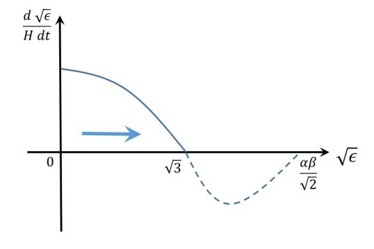
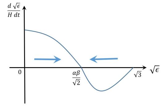
Figure 1: The variation of the rate $\frac{d}{Hdt}\sqrt{\epsilon}$ as a function of $\sqrt{\epsilon}$. Left : For $\alpha\beta>\sqrt{6}$, the positivity of the potential imposes $\sqrt{\epsilon}<\sqrt{3}$, over which $\frac{d}{Hdt}\sqrt{\epsilon}$ is always positive. Then regardless of the initial condition, $\sqrt{\epsilon}$ increases in time and eventually converges to $\sqrt{3}$. Right : For $\alpha\beta<\sqrt{6}$, $\frac{d}{Hdt}\sqrt{\epsilon}$ is negative (positive) for $\frac{\alpha\beta}{\sqrt{2}}<\sqrt{\epsilon}<\sqrt{3}$ ($0<\sqrt{\epsilon}<\frac{\alpha\beta}{\sqrt{2}}$) in which case $\sqrt{\epsilon}$ decreases (increases) in time until it reaches the stable fixed point $\frac{\alpha\beta}{\sqrt{2}}$. The direction of the time evolution of $\sqrt{\epsilon}$ is indicated by the arrow.

To see the time variation of $\epsilon$ in detail, consider the rate

$$\begin{split}\frac{d}{Hdt}\sqrt{\epsilon}&=\frac{1}{\sqrt{2}\alpha}\frac{d}{Hdt}\Big{(}\frac{\dot{u}}{Hu}\Big{)}=\frac{1}{\sqrt{2}\alpha}\Big{[}\frac{\ddot{u}}{H^{2}u}-\Big{(}\frac{\dot{u}}{Hu}\Big{)}^{2}+\epsilon\frac{\dot{u}}{Hu}\Big{]}\\ &=(\sqrt{\epsilon}+\sqrt{3})(\sqrt{\epsilon}-\sqrt{3})\Big{(}\sqrt{\epsilon}-\frac{\alpha\beta}{\sqrt{2}}\Big{)},\end{split}$$ (12)

where (10) is used for the last equality. If $\alpha\beta>\sqrt{6}$, $\frac{d}{Hdt}\sqrt{\epsilon}$ is positive for $0\leq\sqrt{\epsilon}<\sqrt{3}$ and negative for $\sqrt{3}<\sqrt{\epsilon}<\frac{\alpha\beta}{\sqrt{2}}$, but the latter region is not physically meaningful due to the positivity of the potential $V=\frac{V_{0}}{u^{\beta}}$ : see the first equation in (11). As depicted in the left panel of Fig. 1, since $\frac{d}{Hdt}\sqrt{\epsilon}$ is always positive, regardless of the initial value, $\epsilon$ increases in time until it reaches $3$ at which the ratio $\frac{V}{3M_{\rm Pl}^{2}H^{2}}$ becomes $0$. Thus the upper bound on $\epsilon$ given by $3$ can be interpreted as a stable fixed point. We note that this stable fixed point value does not depend on both $\alpha$ and $\beta$. This reflects the fact that for $\alpha\beta>\sqrt{6}$, the potential quickly decreases to $0$ : as $u$ rolls down the potential, the ratio $\frac{V}{3M_{\rm Pl}^{2}H^{2}}$ converges to $0$ (where $\epsilon$ becomes $3$), while both $V$ and $H$ decrease to $0$. In fact, $\alpha\beta$ is nothing more than the decay rate of the potential with respect to the canonically normalized field $\varphi=\frac{M_{\rm Pl}}{\alpha}\log u$ (see (7)). We also note that at $\epsilon=3$, $\frac{\ddot{u}}{H^{2}u}=-(3\sqrt{6}-6\alpha)\alpha$ is not necessarily suppressed compared to $\frac{\dot{u}}{Hu}=\sqrt{6}\alpha$ thus the slow-roll approximation is not guaranteed. More precisely, $|\frac{\ddot{u}}{H^{2}u}|$ is larger than $\frac{\dot{u}}{Hu}$ for $\alpha<\sqrt{\frac{2}{3}}$ and $\alpha>2\sqrt{\frac{2}{3}}$.

On the other hand, when $\alpha\beta=\sqrt{6}$, the value of $\frac{\alpha\beta}{\sqrt{2}}$ at which $\frac{d}{Hdt}\sqrt{\epsilon}=0$ coincides with $\sqrt{3}$, thus $\frac{d}{Hdt}\sqrt{\epsilon}\geq 0$ for any value of $\sqrt{\epsilon}$ in the physical region $0\leq\sqrt{\epsilon}\leq\sqrt{3}$ and $\frac{d}{Hdt}\sqrt{\epsilon}=0$ only at $\epsilon=3$. Then the qualitative feature of the time variation of $\epsilon$ is the same as that in the case of $\alpha\beta>\sqrt{6}$.

Finally, when $\alpha\beta<\sqrt{6}$, $\frac{\alpha\beta}{\sqrt{2}}$ is smaller than $\sqrt{3}$ hence belongs to the physical region. In this case, as can be found in the right panel in Fig. 1, $\frac{d}{Hdt}\sqrt{\epsilon}$ is positive for $0<\sqrt{\epsilon}<\frac{\alpha\beta}{\sqrt{2}}$ and negative for $\frac{\alpha\beta}{\sqrt{2}}<\sqrt{\epsilon}<\sqrt{3}$. Then $\epsilon=\frac{(\alpha\beta)^{2}}{2}$ corresponds to a stable fixed point : if the initial value of $\epsilon$ is smaller (larger) than $\frac{(\alpha\beta)^{2}}{2}$, $\epsilon$ increases (decreases) in time until it becomes $\frac{(\alpha\beta)^{2}}{2}$. Indeed, at the stable fixed point, the Hubble parameter,

$$\begin{split}H(t)=\frac{H(0)}{1+\frac{(\alpha\beta)^{2}}{2}H(0)t},\end{split}$$ (13)

behaves as $H(t)\sim\frac{2}{(\alpha\beta)^{2}}\frac{1}{t}\to 0$ at late time, and at the same time, the potential

$$\begin{split}V=\Big{(}1-\frac{\epsilon}{3}\Big{)}3H^{2}M_{\rm Pl}^{2}=\Big{(}1-\frac{(\alpha\beta)^{2}}{6}\Big{)}3M_{\rm Pl}^{2}\Big{(}\frac{H(0)}{1+\frac{(\alpha\beta)^{2}}{2}H(0)t}\Big{)}^{2}\end{split}$$ (14)

also decreases to zero. That is, while $\sigma$ rolls down the potential, both $V$ and $H^{2}$ decrease to zero with the same rate such that the ratio $\frac{V}{3M_{\rm Pl}^{2}H^{2}}$ is kept constant. We also note that if $\alpha\beta\ll\sqrt{2}$ the stable fixed point value $\epsilon=\frac{(\alpha\beta)^{2}}{2}$ is much smaller than $1$. Then the slow-roll condition is satisfied at late time provided $\frac{\ddot{\sigma}}{H^{2}\sigma}=\alpha^{4}\beta^{2}\big{(}1-\frac{\beta}{2}\big{)}$ is much smaller than $\frac{\dot{\sigma}}{H\sigma}=\alpha^{2}\beta$, in which case $V$ can be approximated by $3M_{\rm Pl}^{2}H(t)^{2}$.

We can compare $\epsilon$ with the ‘potential slow-roll parameter’ given by

$$\begin{split}\epsilon_{V}=\frac{1}{2}M_{\rm Pl}^{2}\Big{(}\frac{\alpha^{2}u^{2}}{M_{\rm Pl}^{2}}\Big{)}\Big{(}\frac{dV/du}{V}\Big{)}^{2}=\frac{(\alpha\beta)^{2}}{2},\end{split}$$ (15)

where $\frac{\alpha^{2}u^{2}}{M_{\rm Pl}^{2}}$ comes from the inverse of the the Kähler metric. Then one finds that if $\epsilon=\epsilon_{V}$, it is nothing more than the value of $\epsilon$ at which $\frac{d}{Hdt}\sqrt{\epsilon}$ becomes $0$. Whether it is a physical stable fixed point depends on the size of $\alpha\beta$. That is, while we can approximate $\epsilon$ by $\epsilon_{V}$ when the slow-roll condition is satisfied, the exact equality $\epsilon_{V}=\epsilon$ is satisfied at the stable fixed point provided $\alpha\beta\leq\sqrt{6}$.

3 Volume modulus and dilaton runaways

We now move onto the contributions of (the scalar part of) the volume modulus and the dilaton to $\epsilon$ in the asymptotic region when only one of them rolls down the potential. For this purpose, we consider the compactification of Type IIB string theory with a single Kähler modulus, the volume modulus $\rho$. In this case, the Kähler potential is given by

$$\begin{split}K/M_{\rm Pl}^{2}=-3\log\big{[}-i(\rho-\overline{\rho})\big{]}-\log\big{[}-i(\tau-\overline{\tau})\big{]}+K_{0}/M_{\rm Pl}^{2},\end{split}$$ (16)

where $\tau$ is the axio-dilaton and $K_{0}$ depends on the complex structure moduli. Meanwhile, the superpotential $W$ is independent of $\rho$ in the absence of the quantum corrections such as the non-perturbative effects. Then the action for the moduli $\phi^{I}$ (which include $\rho$ and $\tau$, as well as the complex structure moduli) is

$$\begin{split}S[\phi^{I}]=\int d^{4}xa^{3}\big{(}K_{I{\overline{J}}}{\dot{\phi}}^{I}{\dot{\overline{\phi}}}^{\overline{J}}-V(\phi^{I})\big{)},\end{split}$$ (17)

where the potential is given by

$$\begin{split}V=e^{K/M_{\rm Pl}^{2}}\Big{(}K^{I{\overline{J}}}D_{I}WD_{\overline{J}}\overline{W}-\frac{3}{M_{\rm Pl}^{2}}|W|^{2}\Big{)},\end{split}$$ (18)

with $D_{I}W=\partial_{I}W+\frac{1}{M_{\rm Pl}^{2}}\partial_{I}K$. Denoting the scalar part of $\rho$ and $\tau$ by $\sigma$ and $s$, respectively (that is, $\rho=i\sigma+\theta$ and $\tau=is+a$), the volume of the internal manifold in string units is given by $\sigma^{3/2}$ and the string coupling constant $g_{s}$ is identified with $s^{-1}$. Since $K^{\rho{\overline{\rho}}}K_{\rho}K_{\overline{\rho}}=3M_{\rm Pl}^{2}$, in the absence of the quantum corrections, the potential exhibits the no-scale structure,

$$\begin{split}V=\frac{e^{K_{0}/M_{\rm Pl}^{2}}}{2s\times 8\sigma^{3}}K^{i\overline{j}}D_{i}WD_{\overline{j}}\overline{W},\end{split}$$ (19)

where $i,j$ run over moduli other than $\sigma$.

3.1 Volume modulus

We first assume that $s$ is stabilized, i.e., the value of $g_{s}$ is fixed, and investigate the rolling of $\sigma$. While the potential can be written as $V(\sigma)=V_{0}/\sigma^{3}$, for the comparison with the more suppressed potential (which violates the no-scale structure), we consider the potential given by $V=V_{0}/\sigma^{3+q}$, where $q\geq 0$. Then the action for $\sigma$ is

$$\begin{split}S_{\sigma}=\int d^{4}xa^{3}\Big{(}\frac{3}{4}M_{\rm Pl}^{2}\frac{\dot{\sigma}^{2}}{\sigma^{2}}-\frac{V_{0}}{\sigma^{3+q}}\Big{)},\end{split}$$ (20)

which is the same form as (6) with $\alpha=\sqrt{\frac{2}{3}}$ and $\beta=3+q$. In other words, the field redefinition for the canonical kinetic term is given by $\varphi=\sqrt{\frac{3}{2}}M_{\rm Pl}\log\sigma$. The slow-roll parameter in this case is given by

$$\begin{split}\epsilon=\frac{2K_{\rho{\overline{\rho}}}\dot{\sigma^{2}}}{2H^{2}M_{\rm Pl}^{2}}=\frac{3}{4}\Big{(}\frac{\dot{\sigma}}{H\sigma}\Big{)}^{2},\end{split}$$ (21)

whereas the potential and $\frac{\ddot{\sigma}}{H^{2}\sigma}$ is written as

$$\begin{split}&\frac{V}{3H^{2}M_{\rm Pl}^{2}}=\frac{V_{0}/\sigma^{3+q}}{3H^{2}M_{\rm Pl}^{2}}=1-\frac{\epsilon}{3},\\ &\frac{\ddot{\sigma}}{H^{2}\sigma}=6\Big{(}1+\frac{q}{3}\Big{)}-2\sqrt{3}\sqrt{\epsilon}-\frac{2}{3}(1+q)\epsilon,\end{split}$$ (22)

respectively.

The values of $\alpha$ and $\beta$ for $\sigma$ satisfy $\alpha\beta=\sqrt{6}\big{(}1+\frac{q}{3}\big{)}$, thus according to the discussion in Sec. 2, the rate of the change of $\sqrt{\epsilon}$ in time is given by

$$\begin{split}\frac{d}{Hdt}\sqrt{\epsilon}&=\frac{\sqrt{3}}{2}\frac{d}{Hdt}\Big{(}\frac{\dot{\sigma}}{H\sigma}\Big{)}=(\sqrt{\epsilon}+\sqrt{3})(\sqrt{\epsilon}-\sqrt{3})\Big{(}\sqrt{\epsilon}-\sqrt{3}\Big{(}1+\frac{q}{3}\Big{)}\Big{)},\end{split}$$ (23)

and the positivity of $V$ imposes that the viable range of $\sqrt{\epsilon}$ is restricted to $0\leq\sqrt{\epsilon}\leq\sqrt{3}$. Since $\frac{d}{Hdt}\sqrt{\epsilon}$ is always positive in this region, as time goes on, $\epsilon$ increases toward the fixed point $\epsilon=3$, which is satisfied at $V=0$, or equivalently, $\sigma=\infty$. Moreover, since the fixed point value $\epsilon=3$ is larger than $1$ and the absolute value of $\frac{\ddot{\sigma}}{H^{2}\sigma}=-2$ is the same as that of $\frac{\dot{\sigma}}{H\sigma}=2$, the slow-roll condition is not satisfied.

The fact that the fixed point value $\epsilon=3$ is independent of the choice of $q$ may be compared to the potential slow-roll parameter

$$\begin{split}\epsilon_{V}=\frac{1}{2}M_{\rm Pl}^{2}\frac{K^{\rho\overline{\rho}}}{2}\Big{(}\frac{dV/d\sigma}{V}\Big{)}^{2}=3\Big{(}1+\frac{q}{3}\Big{)}^{2}.\end{split}$$ (24)

When $q>0$, $\epsilon_{V}$ cannot be the viable value of $\epsilon$ since $\epsilon=\epsilon_{V}$ gives $\frac{V}{3H^{2}M_{\rm Pl}^{2}}=-\frac{q}{3}\big{(}2+\frac{q}{3}\big{)}<0$ (see the first equation in (22)), which is not compatible with the positivity of the potential. Meanwhile, when $q=0$, $\epsilon_{V}$ coincides with the fixed point value $\epsilon=3$. We note that $\epsilon_{V}$ is given by $3$ only if the Kähler potential depends on $\sigma$ as $-3\log[2\sigma]$ (not, say, $-(3+q)\log[2\sigma]$) and $W$ is independent of $\sigma$, or equivalently, the potential exhibits the no-scale structure thus $q$ is exactly $0$. In contrast, the fixed point value of $\epsilon$ is $3$ regardless of the value of $q$, and it indeed originates from the more generic condition, the positivity of the potential (given by the first equation in (11) or (22)), not the no-scale structure.

3.2 Dilaton

We now consider the case in which the value of $\sigma$ is fixed but $s$ rolls down the potential. When the fluxes are turned off, $W$ is independent of $\tau$ (hence $s$) as well, then from $K^{\tau{\overline{\tau}}}K_{\tau}K_{\overline{\tau}}=M_{\rm Pl}^{2}$ the potential can be written as $V=V_{0}/s$. From this, the action for $s$ is given in the form of (6) with $\alpha=\sqrt{2}$ and $\beta=1$,

$$\begin{split}S_{s}=\int d^{4}xa^{3}\Big{(}\frac{1}{4}M_{\rm Pl}^{2}\frac{\dot{s}^{2}}{s^{2}}-\frac{V_{0}}{s}\Big{)},\end{split}$$ (25)

and the redefined field for the canonical kinetic term is $\varphi=\sqrt{\frac{1}{2}}M_{\rm Pl}\log s$. Thus, the equations of motion give the relations

$$\begin{split}&\epsilon=\frac{2K_{\tau{\overline{\tau}}}\dot{s^{2}}}{2H^{2}M_{\rm Pl}^{2}}=\frac{1}{4}\Big{(}\frac{\dot{s}}{Hs}\Big{)}^{2},\\ &\frac{V}{3H^{2}M_{\rm Pl}^{2}}=\frac{V_{0}/s}{3H^{2}M_{\rm Pl}^{2}}=1-\frac{\epsilon}{3},\\ &\frac{\ddot{s}}{H^{2}s}=6-6\sqrt{\epsilon}+2\epsilon,\end{split}$$ (26)

respectively. Since $\alpha\beta=\sqrt{2}<\sqrt{3}$, the rate of change of $\sqrt{\epsilon}$ in time is

$$\begin{split}\frac{d}{Hdt}\sqrt{\epsilon}=\frac{1}{2}\frac{d}{Hdt}\Big{(}\frac{\dot{s}}{Hs}\Big{)}=(\sqrt{\epsilon}+\sqrt{3})(\sqrt{\epsilon}-1)(\sqrt{\epsilon}-\sqrt{3}).\end{split}$$ (27)

This shows that $\epsilon=1$ corresponds to the stable fixed point : at late time $\epsilon$ converges to $1$ regardless of its initial value in the physical region $0\leq\epsilon\leq 3$. From the equations of motion one finds that $\frac{V}{3H^{2}M_{\rm Pl}^{2}}=\frac{1}{3}$ and $\frac{\dot{s}}{Hs}=\frac{\ddot{s}}{H^{2}s}=2$ are satisfied at the fixed point, which indicates that the slow-roll approximation is not valid. We also note that the value of the potential slow-roll parameter

$$\begin{split}\epsilon_{V}=\frac{1}{2}M_{\rm Pl}^{2}\frac{K^{\tau\overline{\tau}}}{2}\Big{(}\frac{dV/ds}{V}\Big{)}^{2}=1\end{split}$$ (28)

coincides with $\epsilon$ at the fixed point.

4 Fixed point in multifield quintessence model

So far we have considered the simplest quintessence model in which only a single scalar field rolls down the runaway potential. When more than two scalar fields $u_{i}$ ($i=1,\cdots,N$) simultaneously roll down the potential, we need to consider the generalized equations of motion,

$$\begin{split}&3M_{\rm Pl}^{2}H^{2}=\sum_{i}\frac{M_{\rm Pl}^{2}}{2\alpha_{i}^{2}}\frac{\dot{u}_{i}^{2}}{u_{i}^{2}}+V,\\ &3M_{\rm Pl}^{2}H^{2}+2M_{\rm Pl}^{2}\dot{H}=-\sum_{i}\frac{M_{\rm Pl}^{2}}{2\alpha_{i}^{2}}\frac{\dot{u}_{i}^{2}}{u_{i}^{2}}+V,\\ &\ddot{u}_{i}+3H\dot{u}_{i}-\frac{\dot{u}_{i}^{2}}{u_{i}}+\sum_{i}\frac{\alpha_{i}^{2}}{M_{\rm Pl}^{2}}u_{i}^{2}\frac{\partial V}{\partial u_{i}}=0,\end{split}$$ (29)

where we assume that the kinetic mixing between fields is absent. Then they lead to

$$\begin{split}&\epsilon=-\frac{\dot{H}}{H^{2}}=\sum_{i}\frac{1}{2\alpha_{i}^{2}}\Big{(}\frac{\dot{u}_{i}}{Hu_{i}}\Big{)}^{2}\equiv\sum_{i}\epsilon_{i},\\ &\frac{V}{3H^{2}M_{\rm Pl}^{2}}=1-\frac{\epsilon}{3},\end{split}$$ (31)

where $\epsilon_{i}=\frac{1}{2\alpha_{i}^{2}}\big{(}\frac{\dot{u}_{i}}{Hu_{i}}\big{)}^{2}$. Moreover, when the potential satisfies $u_{i}\partial_{i}V=-\beta_{i}V$, i.e., exhibits the runaway behavior with respect to each of $u_{i}$, we obtain the relation

$$\begin{split}&\frac{\ddot{u}_{i}}{H^{2}u_{i}}=3\alpha_{i}^{2}\beta_{i}-3\sqrt{2}\alpha_{i}\sqrt{\epsilon_{i}}+2\alpha_{i}^{2}\epsilon_{i}-\alpha_{i}^{2}\beta_{i}\epsilon.\end{split}$$ (32)

Since $\epsilon$, as well as $\epsilon_{i}$, appears in the above equation (see the last term), the dynamics of any one of moduli is affected by that of others. Of course, in the slow roll approximation in which $\frac{\ddot{u}_{i}}{H^{2}u_{i}}$, $\epsilon$, and $\epsilon_{i}$ are suppressed compared to $\sqrt{\epsilon_{i}}$, each of $\epsilon_{i}$ is decoupled from the rest, giving $\epsilon_{i}\simeq\frac{(\alpha_{i}\beta_{i})^{2}}{2}$ provided $\alpha_{i}\beta_{i}\ll 1$.

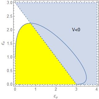
Figure 2: The behavior of the rate $\frac{d\epsilon}{Hdt}$ with respect to $\epsilon_{\sigma}$ and $\epsilon_{s}$. The curve consists of points satisfying $\epsilon=\epsilon_{\sigma}+\epsilon_{s}=\sum_{i}\frac{\alpha_{i}\beta_{i}}{\sqrt{2}}\sqrt{\epsilon_{i}}$. The blue region corresponds to $\epsilon=\epsilon_{\sigma}+\epsilon_{s}>3$, which is excluded by the positivity of the potential. The yellow region satisfies both $\epsilon<3$ and $\epsilon<\sum_{i}\frac{\alpha_{i}\beta_{i}}{\sqrt{2}}\sqrt{\epsilon_{i}}$ (hence $\frac{d\epsilon}{Hdt}>0$). Then the part of the boundary of the yellow region satisfying $\epsilon=\sum_{i}\frac{\alpha_{i}\beta_{i}}{\sqrt{2}}\sqrt{\epsilon_{i}}$ or $\epsilon=3$ consists of the stable fixed points.

In order to find out the fixed points, we consider

$$\begin{split}\frac{d\epsilon}{Hdt}=\sum_{i}\frac{d\epsilon_{i}}{Hdt}&=\sum_{i}\frac{1}{\alpha_{i}^{2}}\Big{(}\frac{\dot{u}_{i}}{Hu_{i}}\Big{)}\Big{(}\frac{\ddot{u}_{i}}{H^{2}u_{i}}-\Big{(}\frac{\dot{u}_{i}}{Hu_{i}}\Big{)}^{2}+\epsilon\frac{\dot{u}_{i}}{Hu_{i}}\Big{)}\\ &=2(\epsilon-3)\Big{(}\epsilon-\sum_{i}\frac{\alpha_{i}\beta_{i}}{\sqrt{2}}\sqrt{\epsilon_{i}}\Big{)},\end{split}$$ (33)

which shows that the stable fixed points are given by

$$\begin{split}\epsilon={\rm min}\Big{[}3,\sum_{i}\frac{\alpha_{i}\beta_{i}}{\sqrt{2}}\sqrt{\epsilon_{i}}\Big{]}.\end{split}$$ (34)

In particular, a set of values $\epsilon_{i}=\frac{(\alpha_{i}\beta_{i})^{2}}{2}$ can be the stable fixed point so far as $\epsilon=\sum_{i}\frac{(\alpha_{i}\beta_{i})^{2}}{2}$ is smaller than $3$ (otherwise, it contradicts to the positivity of the potential). In this case, each of $\epsilon_{i}$ coincides with the contribution of $u_{i}$ to the potential slow roll parameter,

$$\begin{split}\epsilon_{V,i}=\frac{1}{2}M_{\rm Pl}^{2}\Big{(}\frac{\alpha_{i}^{2}u_{i}^{2}}{M_{\rm Pl}^{2}}\Big{)}\Big{(}\frac{dV/du_{i}}{V}\Big{)}^{2}=\frac{(\alpha_{i}\beta_{i})^{2}}{2}.\end{split}$$ (35)

We now investigate the contributions of $\sigma$ and $s$ to $\epsilon$. In this case $(\alpha_{i},\beta_{i})$ ($i=\sigma,s$) are given by $(\sqrt{\frac{2}{3}},3)$ for $\sigma$ and $(\sqrt{2},1)$ for $s$, respectively. From this and $\epsilon=\epsilon_{\sigma}+\epsilon_{s}$ we obtain

$$\begin{split}\frac{d\epsilon}{Hdt}&=2(\epsilon-3)\Big{(}\epsilon-(\sqrt{3}\sqrt{\epsilon_{\sigma}}+\sqrt{\epsilon_{s}})\Big{)}\\ &=2(\epsilon-3)\big{(}\sqrt{\epsilon_{\sigma}}(\sqrt{\epsilon_{\sigma}}-\sqrt{3})+\sqrt{\epsilon_{s}}(\sqrt{\epsilon_{s}}-1)\big{)}.\end{split}$$ (36)

Since the positivity of the potential imposes $\epsilon\leq 3$, $\frac{d\epsilon}{Hdt}$ is positive when both $\epsilon<3$ and $\epsilon<\sqrt{3}\sqrt{\epsilon_{\sigma}}+\sqrt{\epsilon_{s}}$ are satisfied, which corresponds to the yellow region in Fig. 2. Then a set of the stable fixed points is nothing more than the part of the boundary of this region satisfying (34). We note that two curves $\epsilon=3$ and $\epsilon=\sqrt{3}\sqrt{\epsilon_{\sigma}}+\sqrt{\epsilon_{s}}$ intersect at $(\epsilon_{\sigma},\epsilon_{s})=(\frac{3}{4},\frac{9}{4})$ and $(3,0)$, at which $V=0$. Meanwhile, the point $(\epsilon_{\sigma},\epsilon_{s})=(3,1)$ at which $\epsilon_{i}=\epsilon_{V,i}$ is satisfied is excluded by the positivity of the potential. This also indicates that the fixed point value is not necessarily the simple sum of the values obtained in the single field case.

5 Conclusions

In this short note, we consider the stringy quintessence model and investigate the late time contributions of $\sigma$ (the scalar part of the volume modulus) and $s$ (the dilaton) to the slow-roll parameter $\epsilon=-\frac{\dot{H}}{H^{2}}$ which directly measures the deviation of the geometry from dS space. We point out that as time goes on, each of these contributions converges to the stable fixed point, at which the slow-roll approximation does not hold. In particular, in the single field model, it turns out that when the decay rate of the potential is larger than some critical value, the positivity of the potential imposes that the fixed point value is given by $3$, independent of the details of the dynamics. This is somewhat different feature from the potential slow-roll parameter, and $\sigma$ corresponds to this case. When both $\sigma$ and $s$ simultaneously roll down the potential, we can find the curve consisting of the fixed points in the plane of $\epsilon_{\sigma}$ and $\epsilon_{s}$, and as in the single field case, there exists a direction in which the fixed point value of $\epsilon$ is just given by $3$, the maximum value of $\epsilon$. Moreover, unlike the potential slow-roll parameter, the fixed point value in the multifield case is not necessarily given by the sum of fixed point values in the single field case.

The no-go theorem we have investigated indicates that despite the compatibility with the observations, both the metastable dS vacuum and the quintessence suffer from the parametric control problem. It is also remarkable that in order to resolve this problem, we need to understand the dynamics of $\sigma$ and $s$ more clearly. Presumably, there may be an accidental fine-tuning which prevents the instability of $\sigma$ and $s$ (for the instability issue originating from the mixing between $\sigma$ and $s$, see, [42, 43]), or unknown quantum gravity reason which recovers the parametric control.

Acknowledgements

References

• [1]
• [2] N. Aghanim et al. [Planck], Astron. Astrophys. 641 (2020), A6 [erratum: Astron. Astrophys. 652 (2021), C4] [arXiv:1807.06209 [astro-ph.CO]].
• [3] S. Kachru, R. Kallosh, A. D. Linde and S. P. Trivedi, Phys. Rev. D 68 (2003), 046005 [arXiv:hep-th/0301240 [hep-th]].
• [4] V. Balasubramanian, P. Berglund, J. P. Conlon and F. Quevedo, JHEP 03 (2005), 007 [arXiv:hep-th/0502058 [hep-th]].
• [5] M. Dine and N. Seiberg, Phys. Lett. B 162 (1985), 299-302
• [6] U. H. Danielsson and T. Van Riet, Int. J. Mod. Phys. D 27 (2018) no.12, 1830007 [arXiv:1804.01120 [hep-th]].
• [7] G. Obied, H. Ooguri, L. Spodyneiko and C. Vafa, [arXiv:1806.08362 [hep-th]].
• [8] D. Andriot, Phys. Lett. B 785 (2018), 570-573 [arXiv:1806.10999 [hep-th]].
• [9] S. K. Garg and C. Krishnan, JHEP 11 (2019), 075 [arXiv:1807.05193 [hep-th]].
• [10] H. Ooguri, E. Palti, G. Shiu and C. Vafa, Phys. Lett. B 788 (2019), 180-184 [arXiv:1810.05506 [hep-th]].
• [11] A. Hebecker and T. Wrase, Fortsch. Phys. 67 (2019) no.1-2, 1800097 [arXiv:1810.08182 [hep-th]].
• [12] D. Andriot and C. Roupec, Fortsch. Phys. 67 (2019) no.1-2, 1800105 [arXiv:1811.08889 [hep-th]].
• [13] P. J. E. Peebles and B. Ratra, Astrophys. J. Lett. 325 (1988), L17
• [14] B. Ratra and P. J. E. Peebles, Phys. Rev. D 37 (1988), 3406
• [15] R. R. Caldwell, R. Dave and P. J. Steinhardt, Phys. Rev. Lett. 80 (1998), 1582-1585 [arXiv:astro-ph/9708069 [astro-ph]].
• [16] P. Agrawal, G. Obied, P. J. Steinhardt and C. Vafa, Phys. Lett. B 784 (2018), 271-276 [arXiv:1806.09718 [hep-th]].
• [17] M. Cicoli, S. De Alwis, A. Maharana, F. Muia and F. Quevedo, Fortsch. Phys. 67 (2019) no.1-2, 1800079 [arXiv:1808.08967 [hep-th]].
• [18] M. C. David Marsh, Phys. Lett. B 789 (2019), 639-642 [arXiv:1809.00726 [hep-th]].
• [19] A. Hebecker, T. Skrzypek and M. Wittner, JHEP 11 (2019), 134 [arXiv:1909.08625 [hep-th]].
• [20] S. Hellerman, N. Kaloper and L. Susskind, JHEP 06 (2001), 003 [arXiv:hep-th/0104180 [hep-th]].
• [21] W. Fischler, A. Kashani-Poor, R. McNees and S. Paban, JHEP 07 (2001), 003 [arXiv:hep-th/0104181 [hep-th]].
• [22] N. Kaloper and L. Sorbo, Phys. Rev. D 79 (2009), 043528 [arXiv:0810.5346 [hep-th]].
• [23] M. Cicoli, F. G. Pedro and G. Tasinato, JCAP 07 (2012), 044 [arXiv:1203.6655 [hep-th]].
• [24] M. Cicoli, F. Cunillera, A. Padilla and F. G. Pedro, Fortsch. Phys. 70 (2022) no.4, 2200009 [arXiv:2112.10779 [hep-th]].
• [25] M. Cicoli, F. Cunillera, A. Padilla and F. G. Pedro, Fortsch. Phys. 70 (2022) no.4, 2200008 [arXiv:2112.10783 [hep-th]].
• [26] M. Brinkmann, M. Cicoli, G. Dibitetto and F. G. Pedro, JHEP 11 (2022), 044 [arXiv:2206.10649 [hep-th]].
• [27] T. Rudelius, JHEP 10 (2022), 018 [arXiv:2208.08989 [hep-th]].
• [28] J. Calderón-Infante, I. Ruiz and I. Valenzuela, JHEP 06 (2023), 129 [arXiv:2209.11821 [hep-th]].
• [29] F. Apers, J. P. Conlon, M. Mosny and F. Revello, JHEP 08 (2023), 156 [arXiv:2212.10293 [hep-th]].
• [30] G. Shiu, F. Tonioni and H. V. Tran, Phys. Rev. D 108 (2023) no.6, 063527 [arXiv:2303.03418 [hep-th]].
• [31] G. Shiu, F. Tonioni and H. V. Tran, Phys. Rev. D 108 (2023) no.6, 063528 [arXiv:2306.07327 [hep-th]].
• [32] S. Cremonini, E. Gonzalo, M. Rajaguru, Y. Tang and T. Wrase, JHEP 09 (2023), 075 [arXiv:2306.15714 [hep-th]].
• [33] T. Van Riet, [arXiv:2308.15035 [hep-th]].
• [34] M. P. Hertzberg, S. Kachru, W. Taylor and M. Tegmark, JHEP 12 (2007), 095 [arXiv:0711.2512 [hep-th]].
• [35] S. S. Haque, G. Shiu, B. Underwood and T. Van Riet, Phys. Rev. D 79 (2009), 086005 [arXiv:0810.5328 [hep-th]].
• [36] R. Flauger, S. Paban, D. Robbins and T. Wrase, Phys. Rev. D 79 (2009), 086011 [arXiv:0812.3886 [hep-th]].
• [37] C. Caviezel, T. Wrase and M. Zagermann, JHEP 04 (2010), 011 [arXiv:0912.3287 [hep-th]].
• [38] T. Wrase and M. Zagermann, Fortsch. Phys. 58 (2010), 906-910 [arXiv:1003.0029 [hep-th]].
• [39] M. S. Seo, Phys. Rev. D 99 (2019) no.10, 106004 [arXiv:1812.07670 [hep-th]].
• [40] S. Mizuno, S. Mukohyama, S. Pi and Y. L. Zhang, JCAP 09 (2019), 072 [arXiv:1905.10950 [hep-th]].
• [41] H. Ooguri and C. Vafa, Nucl. Phys. B 766 (2007), 21-33 [arXiv:hep-th/0605264 [hep-th]].
• [42] K. Choi, A. Falkowski, H. P. Nilles, M. Olechowski and S. Pokorski, JHEP 11 (2004), 076 [arXiv:hep-th/0411066 [hep-th]].
• [43] M. S. Seo, Nucl. Phys. B 968 (2021), 115452 [arXiv:2103.00811 [hep-th]].