pnassupportinginfo ²To whom correspondence should be addressed. E-mail: paolo.edera@espci.fr; matteo.brizioli@unimi.it; fabio.giavazzi@unimi.it

Yielding under the microscope: a multi-scale perspective on brittle and ductile behaviors in oscillatory shear

Rheology experiments with a commercial rheometer

In addition to using our shear cell rheometer, we conducted rheological experiments using an Anton Paar MCR501 rheometer in strain-controlled mode. The experiments used a rough cone and plate geometry with a diameter of 50 mm, which is crucial for ensuring homogeneous deformation fields, especially in the non-linear regime.

During the experiments, a waveform consisting of stress $\sigma(t)$ and strain $\gamma(t)$ data was recorded every two oscillation cycles. For each shear amplitude, we collected 60 experimental waveforms, equivalent to 120 cycles, to ensure comprehensive data coverage. In the non-linear regime, a transient behavior is observed. Our analysis focuses exclusively on data from the stationary regime The imposed strain is harmonic, while the non-harmonicity of the stress signal is analyzed with a custom code in Matlab as described below.

The stress data represented in the stress-strain curves, $\sigma_{0}(\gamma_{0})$, is sourced directly from the Anton Paar rheometer software, which calculates the amplitude of the first Fourier component of the $\sigma(t)$ signal. Similarly, the viscoelastic moduli reported are those provided by the software, verified to be derived from the amplitude and phase of the first Fourier component of the $\sigma(t)$ signal.

The viscoplastic fragility:

In Ref.(1), both storage and loss moduli are decomposed into solid and liquid components, yielding a total of four moduli. The solid components correspond to elastic or recoverable deformations, while the liquid components account for plastic or unrecoverable deformations. This distinction in the loss modulus helps to separate contributions due to plasticity from those due to other dissipation sources present even in the linear regime. From the liquid part of the loss modulus, the viscoelastic fragility is defined as:

$$N_{F}=\text{max}_{\gamma_{0}}\left[\frac{1}{G^{\prime\prime}_{lin}}\cdot\frac{\partial G^{\prime\prime}_{fluid}}{\partial{\log\gamma_{0}}}\right].$$ (S1)

In traditional oscillatory shear experiments, like ours, it is challenging to access these four moduli directly, as separating recoverable and unrecoverable strain is experimentally complex. However, we assume, as in the cases presented by (1), as we are not able to disentangle the recoverable and unrecoverable strain, a procedure that is quite long and tedious experimentally. However, we assume that also for our samples, as in all the cases presented by (1), that $G^{\prime\prime}_{solid}$ remains nearly constant near the maximum of $G^{\prime\prime}_{fluid}$. Given that $\partial{\log\gamma_{0}}G^{\prime\prime}_{solid}\simeq 0$, it follows that

$$\frac{\partial G^{\prime\prime}}{\partial{\log\gamma_{0}}}\simeq\frac{\partial G^{\prime\prime}_{fluid}}{\partial{\log\gamma_{0}}}.$$ (S2)

Therefore, we compute the viscoplastic fragility using the entire loss modulus, introducing only a minor error.

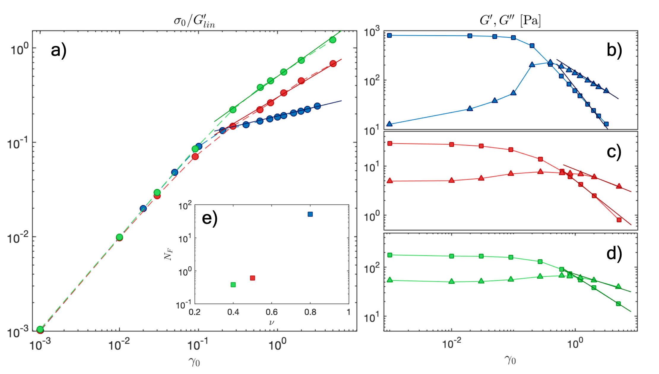
Figure 1: Rheological characterization of the three samples under oscillatory shear. a) Stress-strain curves, normalized for each sample under oscillatory shear, transitioning from linear to power-law regimes $\sigma_{0}\propto\gamma_{0}^{1-\nu}$. Color coding: emulsion (blue), Carbopol 0.5% wt (red), and Carbopol 5% wt (green). (b-d) Storage and loss moduli ($G^{\prime},G^{\prime\prime}$) for each sample, demonstrating typical YSM behavior. The exponent $\nu$ for the terminal regime is derived from a global fit of the moduli as a function of $\gamma_{0}$ and the stress-strain curves (continuous colored lines). (e) Viscoplastic fragility ($N_{F}$) plotted against the terminal flow exponent ($\nu$). The tests are performed in cone plate geometry, ensuring the uniformity of stress throughout all the samples, at a frequency of 1 Hz, with each data point representing a stationary condition achieved after 120 cycles.

Rheomicroscopy experiments with a custom shear cell

A detailed description of the acquisition protocols, processing and analysis of the measurements performed with the custom-built stress-controlled shear cell can be found in refs. (2, 3). Here, we briefly recall some of the acquisition setting parameters, analysis steps, and the most important definitions.

Shear protocol

Before each measurement at a given stress amplitude $\sigma$, the initial mechanical properties of the samples were reset by adopting a rejuvenation or preshear protocol. In particular, samples were presheared by imposing an oscillatory stress profile of $\sim$400 periods at constant frequency starting from a stress amplitude $\sigma_{0}$, for which the measured strain amplitude was around $\gamma_{0}=$ 200-250$\%$, reaching the target stress value $\sigma$ at which the measurement was carried out. After the preshear phase, for each imposed oscillatory stress, we performed 3 acquisitions of duration typically 20-30 oscillation periods from which the strain, hence the rheological response of the material, is estimated. Subsequently, we performed a z-scan with a vertical resolution of $\Delta z$ of 20$\mu$m, starting from the top-plate and moving downwards to the bottom plate. At each plane, we acquired a fast image sequence of the embedded tracers corresponding to typically 4-5 oscillations. Finally, an echo image sequence was acquired by focusing on the middle plane inside the gap for 400 oscillations.

Imaging settings

Image acquisition was performed with a standard optical microscope (Nikon Eclipse Ti), equipped with a 20x, (NA=0.45) objective, keeping the diaphragm completely open (NA=0.52) to minimize the focal depth. Images were acquired with a Ximea MQ042MG-CM USB3.0 camera, with a resolution, upon 2x2 binning, of 512x512 pixels for the z-scan acquisitions and 1024x1024 pixels for the echo sequences. The effective pixel size is $d_{eff}=0.55\mu$m. Thanks to an external trigger, the image acquisition is synchronized with the oscillatory stress profile. We imposed an acquisition rate of 45 frames per cycle for the fast z-scan measurements, while we used a frame rate of 10-15 frames per cycle for the echo sequences.

Deformation profiles

As described in refs. (3, 2), the displacement field $\Delta x(z,t)$ is obtained using an image cross-correlation algorithm. We systematically checked that the recorded displacement field is periodic, corresponding to a stationary regime. The local deformation $\gamma_{L}(z,t)$ is computed as

$$\gamma_{L}(z,t)=\frac{\Delta x(z+\frac{\Delta z}{2},t)-\Delta x(z-\frac{\Delta z}{2},t)}{\Delta z}.$$ (S3)

We note that, while the displacement fields at different heights are not measured simultaneously, we can still compute $\gamma_{L}(z,t)$ thanks to stationarity, as the origin of the intracycle time $t$ is phase-locked to the applied stress for all heights $z$. In Fig.2, we report the amplitude of the deformation profiles $A(z)$ and the estimated local strain amplitude $\gamma_{L}(z)$ for Carbopol 5$\%$ (Fig.2.a-c), the emulsion (Fig.2.d-f), and Carbopol 0.5% (Fig.2.g-i). Repeated measurements on the same sample show that the deformation profile $\gamma_{L}(z)$ is highly reproducible and time-independent (Fig.3). However, different independent experiments, involving unloading and reloading fresh samples into the shear cells, yield variable $\gamma_{L}(z)$ profiles.

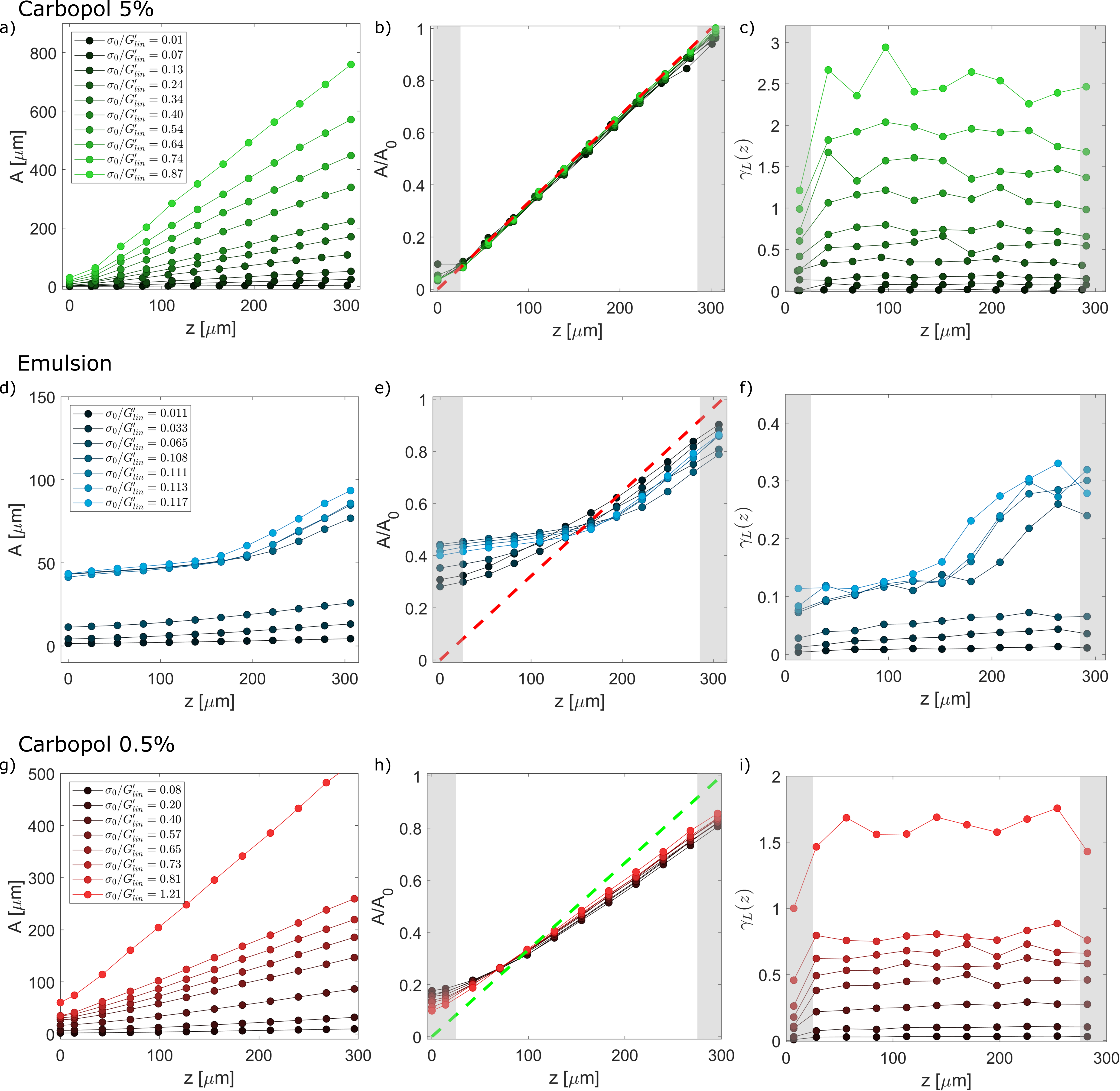
Figure 2: Deformation profiles and local strain amplitude for Carbopol $5\%$, emulsion and Carbopol $0.5\%$. Panels (a-c) refers to Carbopol $5\%$, panels (d-f) to emulsion and panels (g-i) to Carbopol $0.5\%$. (a) Deformation profiles $A(z)$ for different imposed stress amplitudes increasing from black to green. (b) Rescaled amplitudes $A(z)$ with the top plate displacement $A_{0}$ as measured from the shear-cell(2). The red dashed line stands for the ideal case of a homogeneous profile without shear bands and wall-slip. (c) Effective strain amplitude $\gamma_{L}(z)$ in the gap estimated exploiting Eq.S3. (d) Representative deformation profile for emulsion. Colors from black to light blue corresponds to increasing stress amplitude. (e) Normalized deformation profile over the bulk deformation $A_{0}$. (f) Estimated strain amplitude $\gamma_{L}(z)$ across the gap. (g) Representative deformation profile for Carbopol 0.5%. Colors ranging from black to red indicates increasing stress amplitude. (e) Normalized deformation profile over the bulk deformation $A_{0}$, with the green dashed line indicating the expected profile in absence of shear-bands and wall-slip. (f) Local strain amplitude $\gamma_{L}(z)$ across the gap distance.

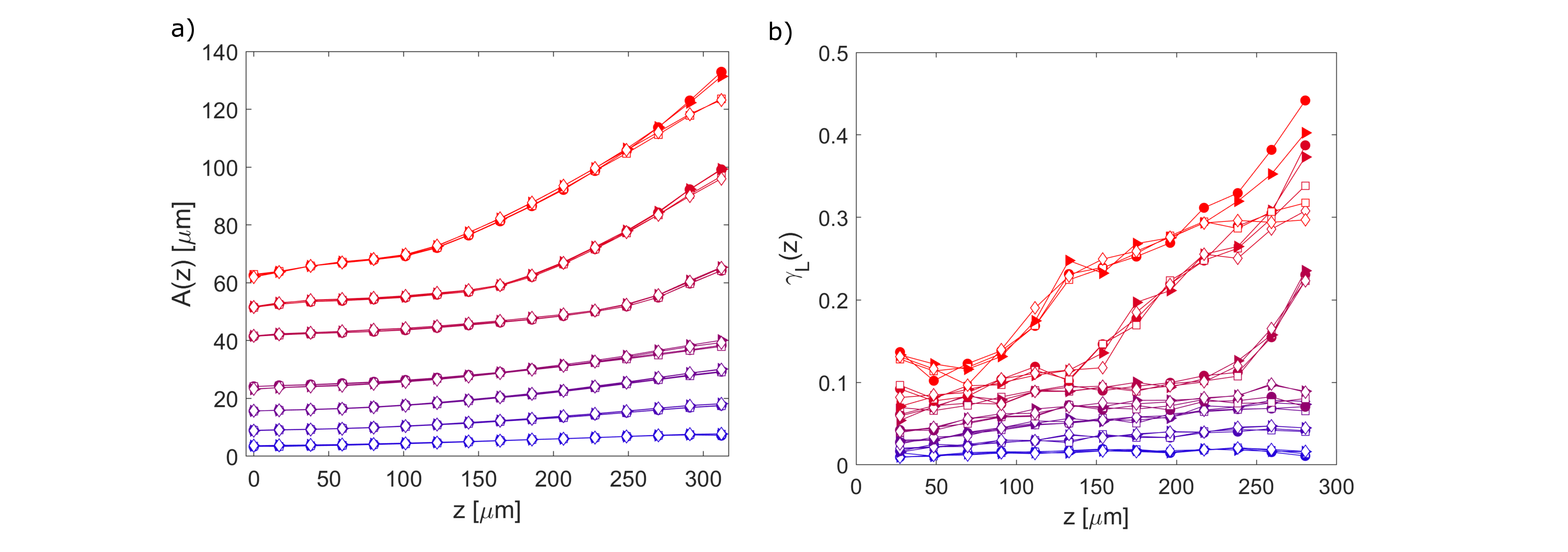
Figure 3: Assessment of repeatability of deformation profile (a) and strain amplitude (b) for the emulsion. The imposed stress amplitude increase from blue to red. To test the repreatibility we performed for each stress amplitude two series of measurements consisting in preshear and subsequent measurements of the deformation profiles by moving downward from the top plate and bottom plate (solid symbols) and then moving upward from the bottom plane to the top one (open symbols). We repeated this protocol two times. Specifically, solid $\bigcirc$ and $\rhd$ stand for 1^st and 2^nd downwards, respectively, whereas open $\Box$ and $\bigtriangledown$ corresponds to 1^st and 2^nd upwards, respectively.

Echo image acquisition and analysis

Echo image acquisition

Our echo acquisition scheme consists of capturing a sequence of evenly spaced images covering many oscillation cycles (typically $\sim$ 400). Within each cycle, an integer number $n_{echo}$ (typically $\sim$ 10) of images is captured. In this way, we obtain $n_{echo}$ different stroboscopic image sequences for each experiment (each one corresponding to a different phase of the oscillatory stress), from which we estimate the non-affine dynamics of the embedded tracers. To identify and correct potential drifts in the images due to mechanical instabilities of the experimental setup or to the imperfect synchronization of the acquisition we adopt the following procedure. For each image sub-sequence, we first subtract a background image, obtained as the median of the entire stack, and we then use a rigid registration algorithm exploiting the Image-J plugin Stack-Reg to identify the global translation that potentially occurred between any pair of consecutive echo images. Such transformation is then used to correct frame by frame the tracer positions identified by a particle tracking algorithm, as detailed in the next subsection.

Echo particle tracking

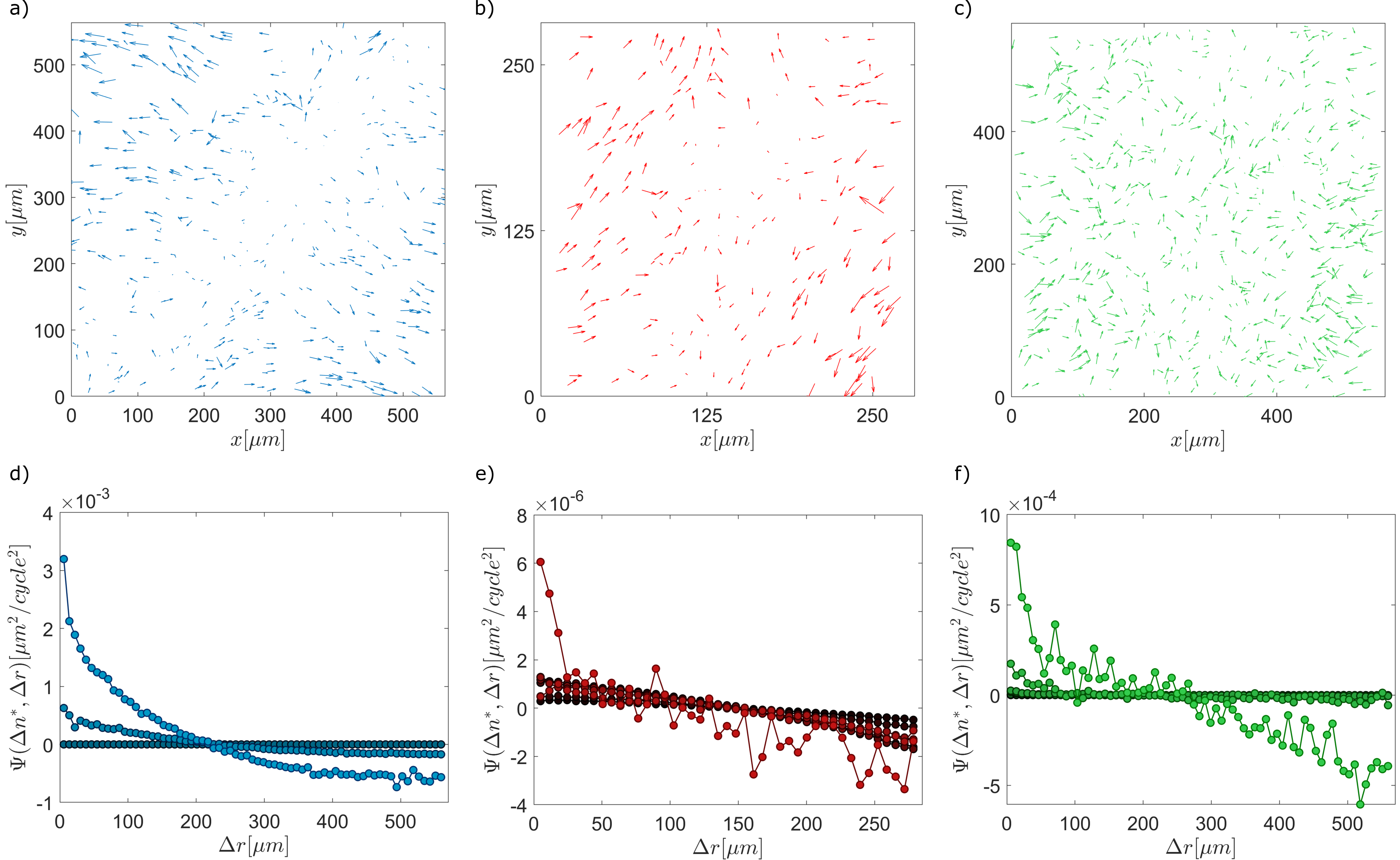
Figure 4: Velocity Correlations for the three samples. (a-c) 2D projection of the single particles velocities for $\Delta n=150s$ average over the initial time for $\sigma_{0}/G^{\prime}_{lin}\simeq 0.093$ (Emulsion), $\sigma_{0}/G^{\prime}_{lin}\simeq 0.27$ (Carbopol 0.5%) and $\sigma_{0}/G^{\prime}_{lin}\simeq 0.23$ (Carbopol 5%), respectively. Vectors are scaled for clarity. (d-f) Azimuthally-averaged Velocity correlator $\Psi(\Delta r,\Delta n^{*})$ as function of the distance for the three samples, evaluated at $\Delta n^{*}$ for which the $\chi_{4}(\Delta n)$ shows a peak. The different colors indicates different stresses, which increase from the darker to the lighter ones.

All the results presented in this paper have been obtained by exploiting a customized version of the MATLAB particle-tracking code originally developed in ref. (4) and available online at https://github.com/dsseara/microrheology. For each stroboscopic sub-sequence, the tracer positions are identified, drift-corrected as explained in the previous subsection and linked to obtain single particle trajectories $[x^{(i)}(n),y^{(i)}(n)]$ (typically $\sim$ 500).

In what follows, the particle trajectories are investigated in the reference frame of the center of mass. In this reference frame, the spatial average of the velocities $\mathbf{v}^{(i)}(n,\Delta n)=[\frac{x^{(i)}(n+\Delta n)-x^{(i)}(n)}{\Delta n},\frac{y^{(i)}(n+\Delta n)-y^{(i)}(n)}{\Delta n}]$ of the particles present in the field of view between cycle $n$ and $n+\Delta n$ is identically zero

$$\sum_{i}^{N}\mathbf{v}^{(i)}(n,\Delta n)=0.$$ (S4)

As can be appreciated from Fig.4.a-c, where representative maps of single particle velocities in the reference frame of the center of mass, spatial correlations are present over the entire image for all the samples. We estimate a characteristic correlation length by considering the velocity-velocity correlation function (5)

$$\Psi(\Delta\mathbf{r},\Delta n)=\langle V(\mathbf{r}+\Delta\mathbf{r};n,\Delta n)V(\mathbf{r};n,\Delta n)\rangle_{n,\mathbf{r}},$$ (S5)

where $\mathbf{V}(\mathbf{r};n,\Delta n)$ is defined as: $\mathbf{V}(\mathbf{r};n,\Delta n)=\sum_{i=1}^{N}\mathbf{v}^{(i)}(n,\Delta n)\delta(\mathbf{r}-\mathbf{r}^{(i)}(n))$. Representative velocity correlation functions for a fixed number of elapsed cycles $\Delta n$ are shown in Fig.4.d-f. For all samples, at short distances, the correlation is positive and then decreases becoming negative at larger distances, with the presence of correlated and anti-correlated domains in all the samples. The presence of at least one zero in the correlation functions is a result of the fact that the average velocity is zero (Eq.S4). The first zero defines a characteristic correlation length that coincides with the average size of the domains. In our case, the occurrences of only two domains (correlated and anticorrelated), with a domain average size of nearly half of the image dimension, suggests the presence of scale-free correlations (5), greater than the typical dimension of the field of view. Since these long-range correlations exceed the typical dimension of our image ROI, we are not able to characterize them. These correlated displacements are more or less pronounced depending on the deformation regime, and they can even dominate the MSD in the intermediate amplitude regime. Observations at lower magnification suggest that these flows are due to edge effects, and thus they are not the interest of our study. To characterize the shear-induced dynamics we focus on the relative displacement between particles, which is less sensitive to this large-scale correlated motion.

Quantification of the non-affine dynamics

MSD and non-Gaussian parameter

To obtain information on the non-affine particle motion removing possible contributions from long-ranged correlated flows, we adopted a relative particle tracking approach (6), which consists of the study of the relative positions between pairs of particles $(i,j)$, whose relative distance is lower than a characteristic distance $|\Delta r|=50\mu m$ that we set by looking at the particle displacement correlations. In this way, we can define the mean squared displacement (MSD) computed over the relative position of the particles $[\Delta x^{(i,j)},\Delta y^{(i,j)}]=[x^{(i)}(n)-x^{(j)}(n),y^{(i)}(n)-y^{(j)}(n)]$, along the vorticity direction as

$$MSD(\Delta n)=\frac{1}{2}\langle|\Delta y^{(i,j)}(n+\Delta n)-\Delta y^{(i,j)}(n)|^{2}\rangle,$$ (S6)

where the average is performed over all pairs of particles and initial cycles. The MSD for a given stress amplitude is then computed by averaging over all the echo phases. We report in Fig.5 the obtained MSD for Carbopol 0.5%.

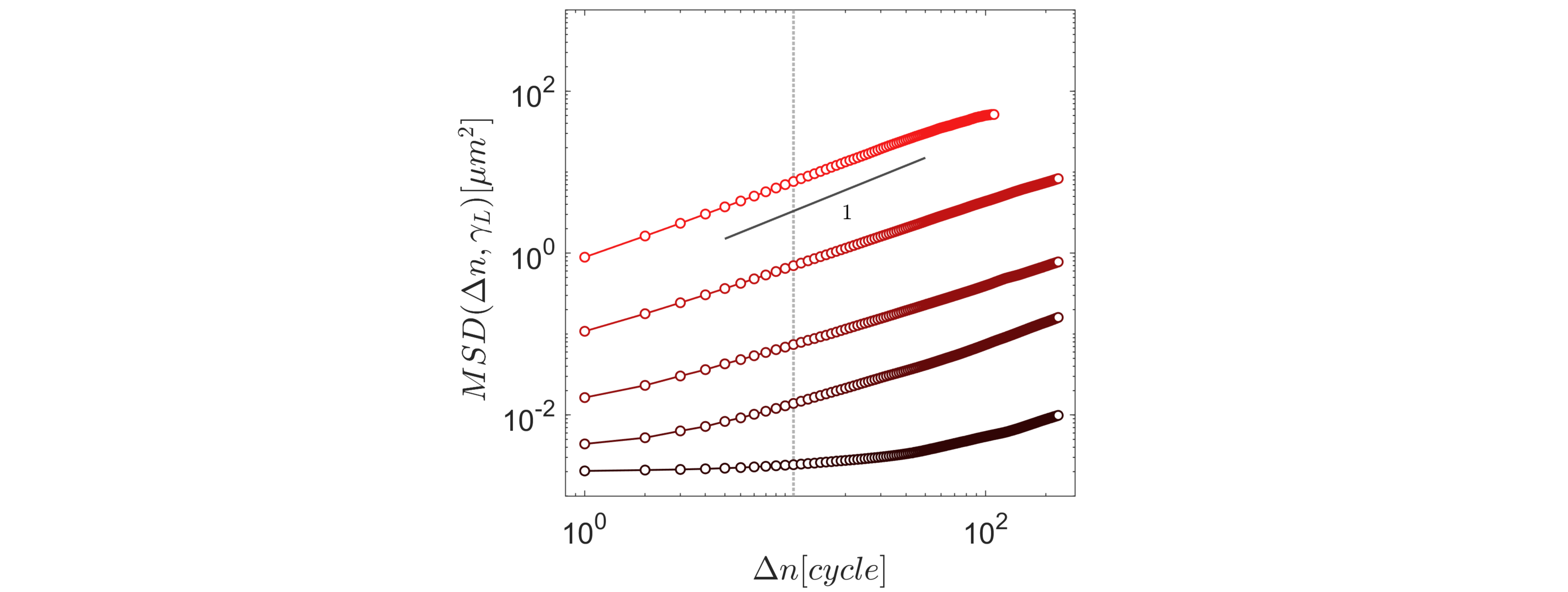
Figure 5: Mutual mean squared displacement (MSD) for Carbopol 0 5% obtained performing oscillatory shear tests at 1 Hz over various local strain amplitudes $\gamma_{L}$ (1.8%, 25%, 30%, 44%, and 73%, with darker to lighter blue indicating increasing strains). MSD is plotted against the number $\Delta n$ of elapsed cycles.

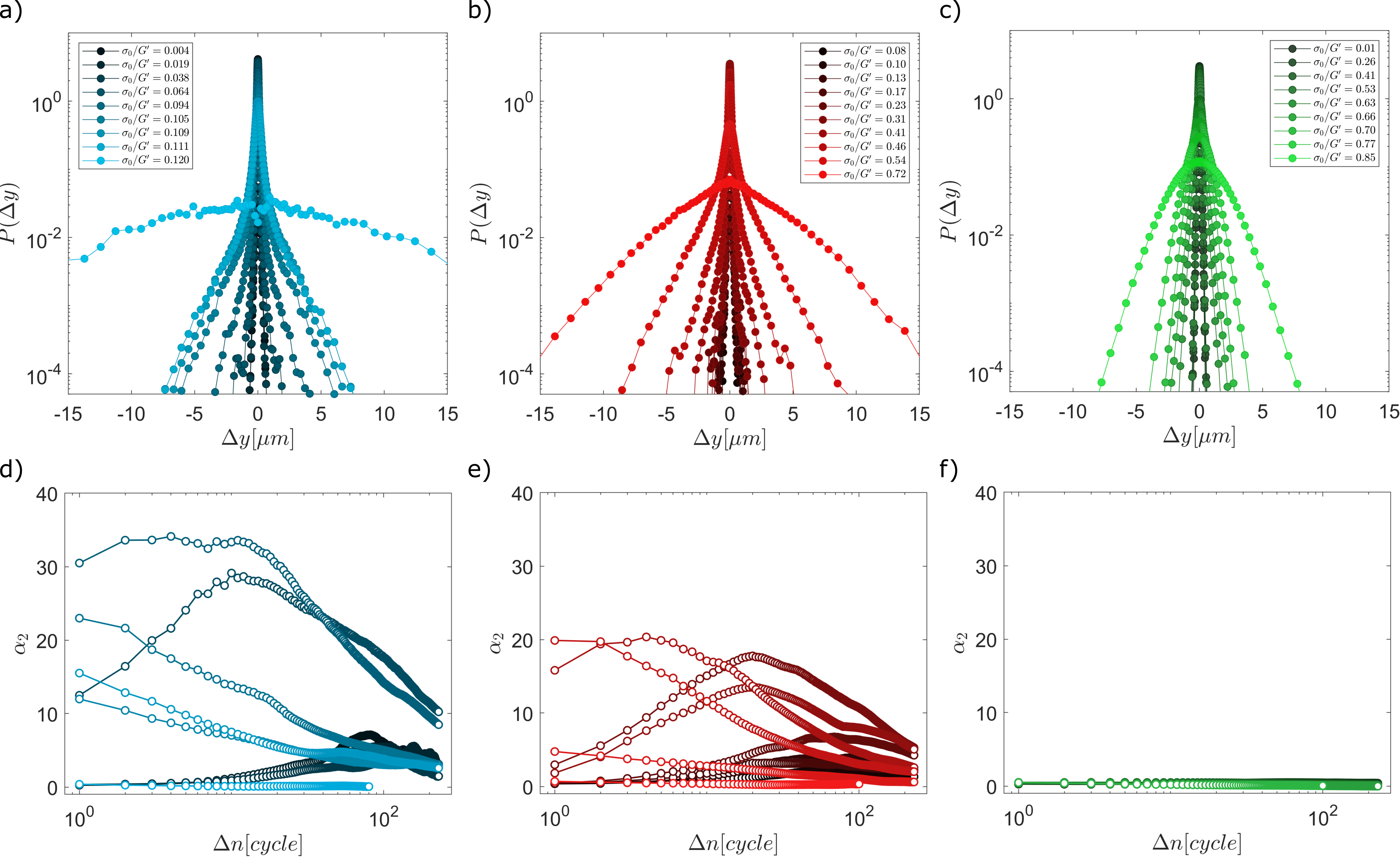
Figure 6: a-c) Mutual-displacement probability distribution functions for the three samples along the vorticity direction for $\Delta n=12$ and different stresses. Colors goes from darker to lighter as the stress increases. d-f) Mutual non-gaussian parameter as a function of time for different applied stress $\alpha_{2}(\Delta n,\gamma^{\prime}_{L})$.In the main text are reported $\alpha_{2}^{*}(\gamma^{\prime}_{L})$: the values at the peak, when this is observed, or the maximum for a fixed stress/strain.

Similarly, from the relative position of the tracers, we evaluate the particle relative displacement probability distribution functions (PDF) along the vorticity $P(\Delta y,\Delta n)$ direction:

$$P(\Delta y,\Delta n)=\langle\delta[\Delta y-(\Delta y^{(i,j)}(n+\Delta n)-\Delta y^{(i,j)}(n))]\rangle,$$ (S7)

where $\delta$ is the Dirac’s delta function. Representative PDFs at a given time for different imposed stresses are shown in Fig.6.a-c. As can be noticed, the tails of the PDFs for the case of the emulsion and the Carbopol 0.5$\%$ are highly non-Gaussian. In order to properly quantify non-Gaussianity, we estimated the one-dimensional non-Gaussian parameter $\alpha_{2}$ as:

$$\alpha_{2}(\Delta n)=\frac{1}{3}\frac{\langle|\Delta y^{(i,j)}(n+\Delta n)-\Delta y^{(i,j)}(n)|^{4}\rangle}{\langle|\Delta y^{(i,j)}(n+\Delta n)-\Delta y^{(i,j)}(n)|^{2}\rangle^{2}}-1.$$ (S8)

The non-Gaussian parameter as a function of the elapsed cycles, for different imposed stresses, is reported in Fig.6.d-f.

Definition of the scaling factor $\lambda$

As mentioned in the main text, independent repetitions of the same experiment upon removing from the cell and re-loading a given sample result in slight variations of both macroscopic and microscopic variables (Fig.7 a-c). Concerning $G^{\prime}$ and $G^{\prime\prime}$, different experiments requires the introduction of a shift factor $\beta\sim 1$ along the vertical axes, this is the consequence of an error in the sample section measurement and ultimately in the conversion from force to stress. The vertical rescaling is not sufficient to lead to a perfect collapse of the data, a further sample-dependent horizontal scaling factor $\lambda$ is introduced to correct for minor discrepancy that can be attributed to sample-to-sample variability. When represented against the rescaled variable $\gamma^{\prime}_{L}=\lambda\cdot\gamma_{L}$ the overlap of the data is optimized both for diffusion coefficient and for the dynamic moduli 7 b-d.

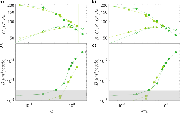
Figure 7: Definition of the rescaled strain $\gamma^{\prime}_{L}$. (a) Viscoelastic moduli (a) and diffusion coefficient (b) obtained from two different loadings of the same sample (circles and squares, respectively). In this caseCarbopol 5$\%$. The continuous lines in (a) indicate the strain amplitudes $\gamma_{L}$ of the crossover points of $G^{\prime}$ and $G^{\prime\prime}$ for the two different repetitions, light green for squares and dark green for circles. (c) Same data of (a) horizontally rescaled by $\lambda$. The moduli are also rescaled vertically by a factor $\beta\simeq 1$. (d) Diffusion coefficient as a function of the rescaled strain amplitude $\gamma^{\prime}_{L}=\lambda\cdot\gamma$. All the measurements have been performed at $\omega=2\pi$ [rad/s]

Stokes-Einstein-like dependence of the shear-induced diffusion coefficient on the tracer radius for the emulsion

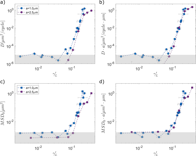
Figure 8: GSER relation for emulsion. Diffusion coefficient $D$ (a) and $MSD_{0}$ (c) as a function of the local strain amplitude $\gamma^{\prime}_{L}$ for two different tracer radius $a=1$ $\mu$m (blue circles) and, $2.5$ $\mu$m (purple circles) . (b,d) Same data as in (a,c) vertically rescaled with the tracer’s radius. All the measurements have been performed at $\omega=2\pi$ rad/s.

Similarly to the case of homogeneous yielding, the tracer’s shear-induced diffusivity in the emulsion displays the same Stokes-Einstein-like dependence on the tracer radius $D\sim 1/a$, and, surprisingly, $MSD_{0}$ also shows the same systematic dependence on the radius $MSD_{0}\sim 1/a$ (8). As pointed out in the main text, this behavior is similar to the Generalize-stokes-Einstein relation (GSER). It indicates that the $MSD$ is strictly related to the effective properties of the materials. We stress that the absence of any motion of the tracers in the quiescent state, along with the stoke-Einstein-like dependence of the mobility on the radius suggests that all the tracer sizes employed in this work are larger than the characteristic microstructural scales of the material. In a previous study (3), we investigated the mobility of smaller tracers with radius $a<0.25$ $\mu$m in similar materials observing thermal motion at rest.
Despite the Stokes-Einstein-like behavior for the $MSD$, we observe that the pdf of tracer displacement changes qualitatively with the tracer size, indicating that particles of different sizes could display distinct behaviors when higher-order indicators are considered, like, for example, the non-Gaussian parameter $\alpha_{2}$. Specifically, if we consider the case of the emulsion, we observe that the distribution for particle of radius $a=2.5$ $\mu$m (purple squares) and $a=1.0$ $\mu$m (Fig.9.b-c) are different, even considering a condition of similar mobility, hence, the rescaled (by the radius) $MSD$s are almost identical (Fig.9.a). Inspection of the distribution probability for the smaller tracers reveals a highly dispersed behavior, with a central region (for small displacements) evolving slowly with the number of elapsed cycle $\Delta n$ as compared to the tails. By contrast, the PDFs for the larger tracers exhibits a more regular behavior with the distribution all broadening over $\Delta n$ while still remaining highly non Gaussian. This suggests that the smaller particles are more sensitive to the heterogeneity of the material. However, quite remarkably, despite the difference in the details of the distributions, the $MSD$ (the variance of the distribution) appears to be independent from these details. This reinforce our claim regarding the $MSD$ as a descriptor of the material’s effective properties. In addition, we checked that the $\chi_{4}$ peak values and their behaviors as a function of the strain amplitude for the bigger tracers is similar to those of the smaller tracers the one of the smaller tracers. Therefore, as for the mean squared displacement also the $\chi_{4}$ is independent of the tracer size and is closely connected to the material properties.

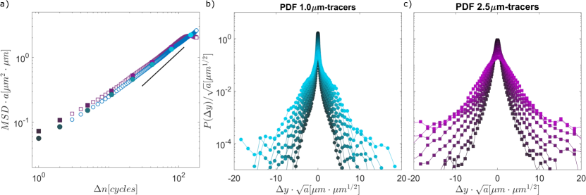
Figure 9: emulsion. (a) Shear induced MSD rescaled with tracers’ radius. Large circles (squares) correspond to $\Delta n$ whose PDFs are shown in panels (b and c). The black line has slope 1 and indicates a diffusive behavior. Representative distribution probability for different number of elapsed cycles (increasing from darker to lighter colors) of two different echo-experiments performed exploiting tracers size (c) $a=2.5$ $\mu$m (purple squares) and (b) $a=1.0$ $\mu$m (blue circles). The mobility for the two selected acquisitions is almost the same, as can be observed from the $MSD$ in (a). Specifically, the local strains are $\gamma^{\prime}_{L}=0.15$ and $\gamma^{\prime}_{L}=0.16$ for (b) and for (c), respectively. All the measurements have been performed at $\omega=2\pi$ rad/s.

Dynamic heterogeneity

As shown in Fig.10.a-c, tracer particles can display a broad spectrum of behaviors, with trajectories differing widely from each other under the same applied stress. In particular, some particles display highly intermittent displacements, with localized sudden jumps, while other particles are nearly immobile. This is a first indication of the presence of dynamic heterogeneity and temporal intermittency, which can be quantitatively captured by considering high-order temporal and spatial correlations(7).

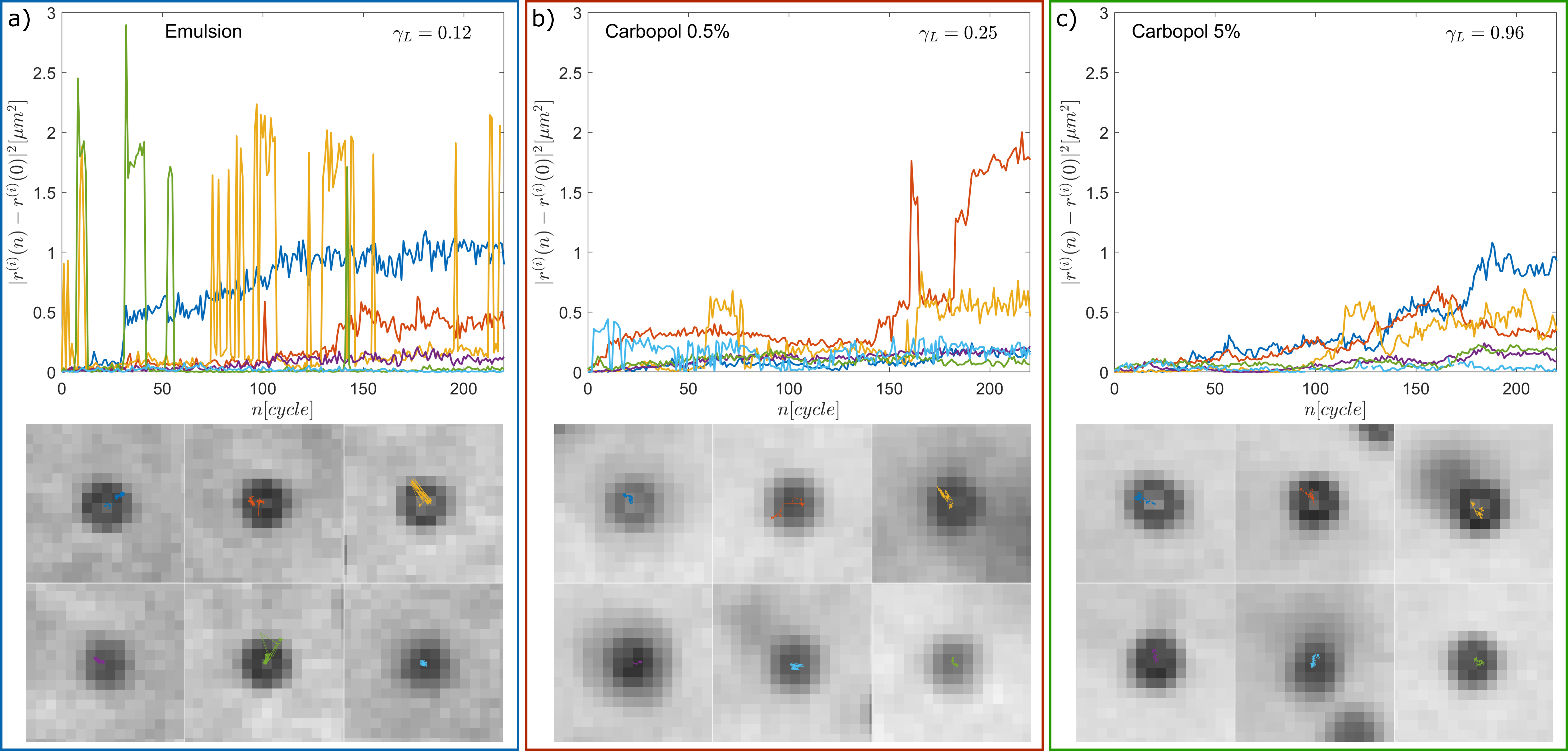
Figure 10: Single particle trajectories for the three samples. Color scale is the same as in the main text. a-c) Top panel: time-resolved square displacement of representative particles trajectories during oscillatory shear for a given local strain amplitude $\gamma_{L}$= 0.12, 0.25, 0.65 for Emulsion, Carbopol 0.5$\%$ and Carbopol 5$\%$, respectively. In the bottom panels, images of the particles shown in the respective upper panel, the colored lines mark the particle trajectories.

To quantify the correlations in real space, one can define a mobility field $c(\mathbf{r};n,\Delta n)$ for a system of $N$ particles, as

$$c(\mathbf{r};n,\Delta n)=\frac{1}{N}\sum_{i=1}^{N}o^{(i)}(n,\Delta n)\delta(\mathbf{r}-\mathbf{r}^{(i)}(n)),$$ (S9)

where $o^{(i)}(n,\Delta n)$ is an overlap function, which quantifies how much a particle has moved along the vorticity direction between cycle $n$ and $n+\Delta n$

$$o^{(i)}(n,\Delta n)=exp\Big{\{}-\frac{(y^{(i)}(n+\Delta n)-y^{(i)}(n))^{2}}{d^{2}}\Big{\}},$$ (S10)

with $d$ being a characteristic distance, typically of the order of the particle size. The degree of the dynamic heterogeneity can be defined as the deviation from the average behavior of the particle mobility. Therefore by defining the total mobility $C(n,\Delta n)=\int d^{2}\mathbf{r}c(\mathbf{r};n,\Delta n)$, we can compute its variance to get the dynamic susceptibility $\chi_{4}(\Delta n)$:

$$\chi_{4}(\Delta n)=N[\langle C(n,\Delta n)^{2}\rangle-\langle C(n,\Delta n)\rangle^{2}],$$ (S11)

which is a measure of the degree of dynamic heterogeneity. Although computationally very efficient, this definition of $\chi_{4}(\Delta n)$ is based on a single-particle approach and it is strongly affected by the presence of long-range correlations in the displacement field, which could lead to an overestimate of $\chi_{4}(\Delta n)$.

The dynamic susceptibility can be also computed starting from the ’four-point’ dynamic correlation function:

$$G_{4}(\Delta\mathbf{r},\Delta n)=\langle c(\mathbf{r}+\Delta\mathbf{r};n,\Delta n)c(\mathbf{r};n,\Delta n)\rangle_{n,\textbf{r}}-\langle c(\mathbf{r};n,\Delta n)\rangle_{n,\mathbf{r}}^{2},$$ (S12)

which measures the spatial and temporal correlations between pairs of particles at a certain separation distance $\Delta r$ and for a certain number of elapsed cycles $\Delta n$. By integrating over the separation distance $\Delta\mathbf{r}$, we can retrieve the dynamic susceptibility:

$$\chi_{4}(\Delta n)=\int d^{2}\Delta\mathbf{r}G_{4}(\Delta\mathbf{r},\Delta n).$$ (S13)

In this work, the presence of large-scale velocity correlations (Fig.10.d-f), prevents the correlator $G_{4}(\Delta r,\Delta t)$ (Fig.11.a-c) decaying to zero for large distances, as one would have expected. To correct for this effect in the evaluation of the $\chi_{4}(\Delta n)$, we subtracted a baseline to the four point correlator obtained by averaging over distances for which it has a plateau, (typically for $r>200\mu$m). The so-obtained new correlator is then integrated using Eq. S13 to get a $\chi_{4}$ cleaned from spurious correlations (fig.11d-f):

$$\chi_{4}(\Delta n)=\int d^{2}\Delta\mathbf{r}[G_{4}(\Delta\mathbf{r},\Delta n)-G_{4}(\Delta\mathbf{r}>200\mu m,\Delta n)].$$ (S14)

For all the experiments in this work, we set $d=0.15\ \mu$m as the characteristic distance for the evaluation of the overlap parameter. This value has been chosen by considering different distances $d$ in a range from 0.01 $\mu$m to 1.0 $\mu$m and taking the value of $\bar{d}$ for which the $\chi_{4}(\Delta n)$ was maximum, together with, the condition of the existence of an interval around $\bar{d}$ for which $\chi_{4}(\Delta n)$ exhibited no change in the functional form with $\Delta n$. Finally, to compare different experiments and samples, we normalized the $\chi_{4}$ with the surface density of the particles $\phi$ in the field of view.

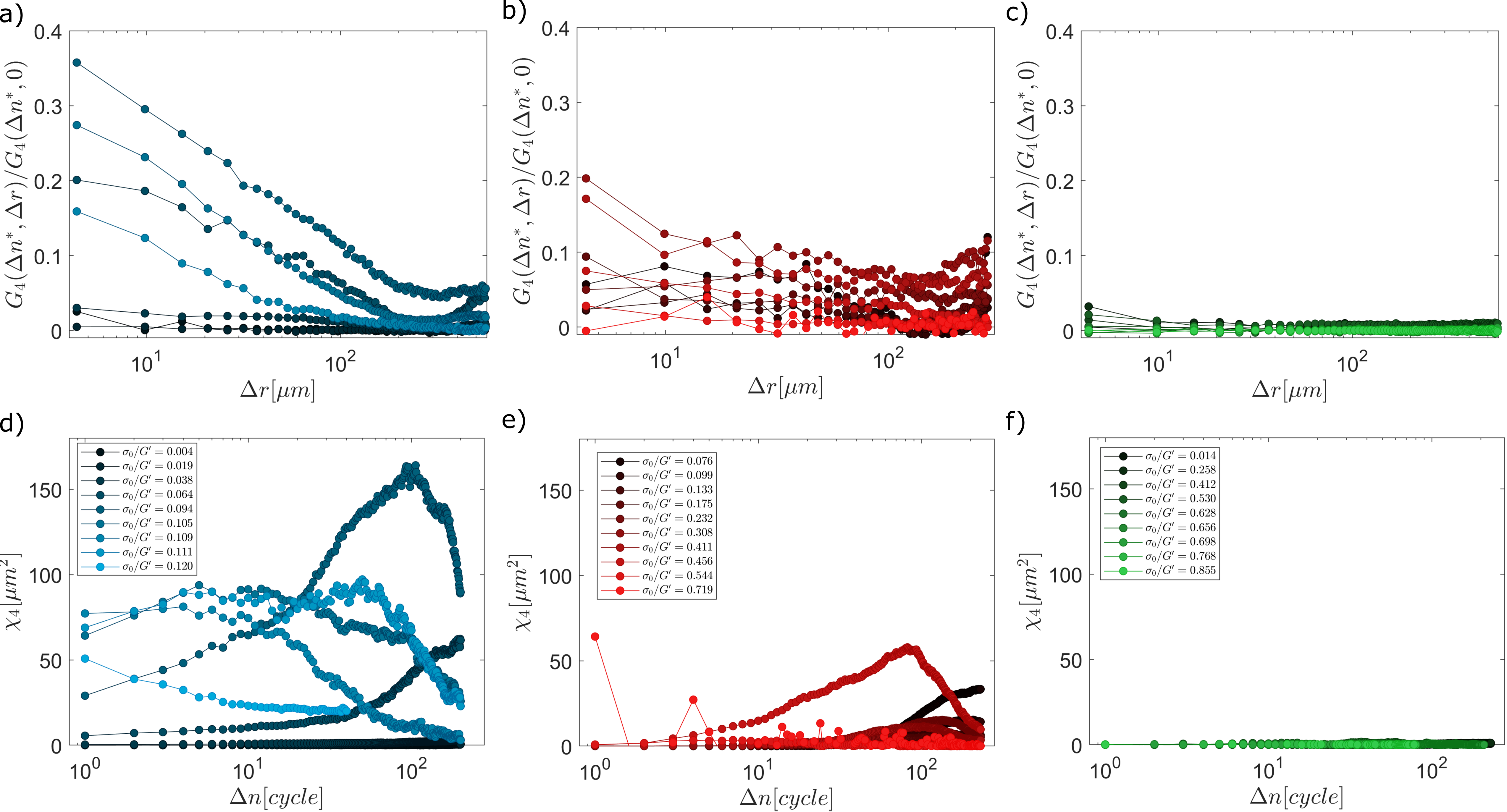
Figure 11: Dynamical heterogeneity for the three samples. a-c) Normalized four-point correlator $G_{4}(\Delta r,\Delta n^{*})$ as a function of the distance for the three samples, evaluated at $\Delta n^{*}$ for which the $\chi_{4}(\Delta n)$ shows a peak. The different colors indicate different applied stresses, which increase from the darker to the lighter ones.

References

- (1) GJ Donley, PK Singh, A Shetty, SA Rogers, Elucidating the g” overshoot in soft materials with a yield transition via a time-resolved experimental strain decomposition. \JournalTitleProceedings of the National Academy of Sciences 117, 21945–21952 (2020).
- (2) S Villa, et al., Quantitative rheo-microscopy of soft matter. \JournalTitleFrontiers in Physics p. 905 (2022).
- (3) P Edera, et al., Deformation profiles and microscopic dynamics of complex fluids during oscillatory shear experiments. \JournalTitleSoft Matter 17, 8553–8566 (2021).
- (4) V Pelletier, N Gal, P Fournier, ML Kilfoil, Microrheology of microtubule solutions and actin-microtubule composite networks. \JournalTitlePhysical review letters 102, 188303 (2009).
- (5) A Cavagna, et al., Scale-free correlations in starling flocks. \JournalTitleProceedings of the National Academy of Sciences 107, 11865–11870 (2010).
- (6) W Pönisch, V Zaburdaev, Relative distance between tracers as a measure of diffusivity within moving aggregates. \JournalTitleThe European Physical Journal B 91, 1–7 (2018).
- (7) L Berthier, Dynamic heterogeneity in amorphous materials. \JournalTitlearXiv preprint arXiv:1106.1739 (2011).