Penalized G-estimation for effect modifier selection in a structural nested mean model for repeated outcomes

Abstract

Effect modification occurs when the impact of the treatment on an outcome varies based on the levels of other covariates known as effect modifiers. Modeling of these effect differences is important for etiological goals and for purposes of optimizing treatment. Structural nested mean models (SNMMs) are useful causal models for estimating the potentially heterogeneous effect of a time-varying exposure on the mean of an outcome in the presence of time-varying confounding. A data-driven approach for selecting the effect modifiers of an exposure may be necessary if these effect modifiers are a priori unknown and need to be identified. Although variable selection techniques are available in the context of estimating conditional average treatment effects using marginal structural models, or in the context of estimating optimal dynamic treatment regimens, all of these methods consider an outcome measured at a single point in time. In the context of an SNMM for repeated outcomes, we propose a doubly robust penalized G-estimator for the causal effect of a time-varying exposure with a simultaneous selection of effect modifiers and use this estimator to analyze the effect modification in a study of hemodiafiltration. We prove the oracle property of our estimator, and conduct a simulation study for evaluation of its performance in finite samples and for verification of its double-robustness property. Our work is motivated by and applied to the study of hemodiafiltration for treating patients with end-stage renal disease at the Centre Hospitalier de l’Université de Montréal. We apply the proposed method to investigate the effect heterogeneity of dialysis facility on the repeated session-specific hemodiafiltration outcomes.

Keywords: G-estimation, penalization, double robustness, effect modifier selection, longitudinal observational data, hemodiafiltration

1 Introduction

When our goal is to estimate the causal effect of a treatment or an exposure on an outcome, effect modification or heterogeneity in the treatment effect may be of interest. Effect modification occurs when the effect of a treatment on an outcome differs according to the level of some other variables, usually pre-treatment covariates; such variables are called effect modifiers (EMs) (VanderWeele and Robins, , 2007). Modeling of these effect differences is important for etiological goals and for purposes of optimizing treatment. Effect modification analysis has gained attention in recent years because of the familiarization with precision medicine (Ashley, , 2015) and dynamic treatment regimes (Murphy, , 2003; Chakraborty and Moodie, , 2013; Chakraborty and Murphy, , 2014; Wallace and Moodie, , 2015), which deal with personalizing treatments by incorporating patient-level information to optimize expected outcomes. Structural nested mean models (SNMMs) are useful causal models for estimating the potentially heterogeneous effect of a time-varying exposure on the mean of an outcome in the presence of time-varying confounding (Robins, , 1989, 1997; Robins et al., , 2007).

Our methods development is motivated by an application in nephrology regarding patients with end-stage renal disease, which is the final, permanent stage of chronic kidney disease. Patients with end-stage renal failure must undergo a kidney transplant or regular dialysis to survive for more than a few weeks. Hemodiafiltration is a dialysis technique that combines diffusive clearance and convective removal of solutes (Ronco and Cruz, , 2007). Hemodiafiltration is the routine dialysis modality for patients with end-stage renal disease treated at the University of Montreal Hospital Centre (CHUM) outpatient dialysis clinic and its affiliated ambulatory dialysis center (CED). The effectiveness of hemodiafiltration is indicated by the convection volume (or total ultrafiltration volume), which is calculated as the sum of the substitution volume and the ultrafiltration volume for weight loss (Marcelli et al., , 2015). The CONvective TRAnsport STudy (CONTRAST) (Grooteman et al., , 2012) randomized controlled trial and a meta-analysis of individual patient-level data from randomized controlled trials showed that hemodiafiltration, compared to hemodialysis, reduced the risk of all-cause mortality by approximately 22%, and of cardiovascular disease mortality by 31%, over a median follow-up of 2.5 years in the hemodiafiltration treatment subgroup achieving high convection volumes (Peters et al., , 2016). These results suggest that one should aim for a convection volume of at least 24 liters per session (Chapdelaine et al., , 2015). On average, convection volumes recorded at the outpatient dialysis clinic located at the CHUM are lower than those at its affiliated ambulatory dialysis center. This has triggered an interest in investigating if there is any effect of the dialysis facility (CHUM vs. CED) on the convection volume or for which patients such an effect exists. Available data from hospital records include sociodemographic information, diagnoses, medications, blood test results, and dialysis treatment parameters of all dialysis sessions per patient in the study time frame (March 1st, 2017 to December 1st, 2021). Convection volume outcomes are available at the end of each successful dialysis session, enabling us to investigate the average effect of the dialysis facility on the session-specific mean convection volume. Since it is currently unknown which measured variables could modify an effect of the dialysis facility on the hemodiafiltration outcome, we thus aim to develop a data-adaptive approach to selecting effect modifiers in this context.

Effect modifier selection is important in the development of optimal dynamic treatment regimes, when not all of the information measured from a patient is necessary for predicting the optimal treatment (Bian et al., , 2021). When comparing multiple treatment strategies, a strategy that uses fewer tailoring variables might be preferred among all other strategies, producing similar performance in terms of patient benefit. Such a preference could be the result of the elimination of the covariates, which are costly and time-consuming to measure and/or burdensome to collect. When covariate dimensionality is high, a data-driven approach for selecting the tailoring variables may be necessary to develop a tractable model (Moodie et al., , 2023). Data-driven variable selection is also of interest if effect modifiers of an exposure are a priori unknown and need to be identified.

Variable selection techniques are available in estimation of the average causal effect (Shortreed and Ertefaie, , 2017; Koch et al., , 2018; Tang et al., , 2022), the conditional average treatment effects using marginal structural models (Bahamyirou et al., , 2022), and in developing optimal dynamic treatment regimens (Gunter et al., , 2011; Shi et al., , 2018; Wallace et al., , 2019; Bian et al., , 2021; Jones et al., , 2022; Bian et al., , 2023; Moodie et al., , 2023). All of these methods were largely developed with an outcome measured at a single point in time. Under a traditional semiparametric regression approach (targeting prediction), Johnson et al., (2008) proposed penalized estimating equations for variable selection with a univariate outcome, whereas Wang et al., (2012) extended this work to high-dimensional longitudinal data proposing penalized generalized estimating equations. Boruvka et al., (2018) discussed assessments of causal effect moderation (modification) in mobile health interventions, where treatment, response and potential moderators are all time-varying. However, to the best of our knowledge, no method exists that conducts simultaneous variable selection and causal effect estimation with longitudinal data and repeated outcomes. Motivated by our application, we seek to develop a doubly robust estimator for the causal effect of a treatment with simultaneous selection of effect modifiers in the SNMM for repeated outcomes.

This paper is organized as follows. In Section 2, we introduce the notation, describe the model and assumptions, present methodological details, and provide theoretical results for the asymptotic properties of the proposed estimator. We present a simulation study to evaluate the performance of our estimator in finite samples in Section 3, and describe the application of the proposed method to the hemodiafiltration data in Section 4. Finally, we provide a discussion in Section 5.

2 Methodology

2.1 Notation and model with assumptions

Suppose we have data from $n$ patients and all patients have measurements from $J$ different hemodiafiltration sessions. At each session, the information of the outcome, the treatment received, and pre-session covariates are recorded. For patient $i$ at session $j$, denote the observed continuous outcome by $Y_{ij}$, the (binary) treatment received by $A_{ij}$, and the vector of covariates by $\bm{\mathbf{L}}_{ij},\forall i=1,\dots,n,j=1,\dots,J$. Let $\bm{\mathbf{H}}_{ij}$ represent the histories of covariates $\bar{\bm{\mathbf{L}}}_{ij}=\{\bm{\mathbf{L}}_{i1},\ldots\bm{\mathbf{L}}_{ij}\}$, past exposures $\bar{A}_{i(j-1)}=\{A_{i1},\ldots,A_{i(j-1)}\}$ and past outcomes $\bar{Y}_{i(j-1)}=\{Y_{i1},\ldots,Y_{i(j-1)}\}$. Throughout this paper, we use the counterfactual framework (Robins, , 1989). Define $Y_{ij}(\bar{a}_{j})$ as the counterfactual outcome that would have been observed at occasion $j$ for patient $i$ if the treatment history $\bar{A}_{ij}=\{A_{i1},\ldots,A_{ij}\}$ were set counterfactually to $\bar{a}_{j}=\{a_{1},\ldots,a_{j}\}$. To model the proximal (short-term) effects of the exposure, a linear SNMM can be defined as (Robins, , 1989; Vansteelandt and Joffe, , 2014)

$$E\{Y_{ij}(\bar{a}_{j-1},a_{j})-Y_{ij}(\bar{a}_{j-1},0)|\bm{\mathbf{H}}_{ij}=\bm{\mathbf{h}}_{ij},A_{ij}=a_{j}\}=\gamma_{j}^{*}(a_{j},\bm{\mathbf{h}}_{ij};\bm{\mathbf{\psi}})$$ (1)

for each measurement occasion $j=1,\ldots,J$, where $\gamma_{j}^{*}(a_{j},\bm{\mathbf{h}}_{ij};\bm{\mathbf{\psi}})$, known as “treatment blip”, is a scalar-valued function smooth in $\bm{\mathbf{\psi}}$; $\bm{\mathbf{h}}_{ij}$ represent the realized values for $\bm{\mathbf{H}}_{ij}$; and $\bm{\mathbf{\psi}}=(\psi_{0},\psi_{1},\ldots,\psi_{K-1})^{\top}$ is a K-dimensional vector of parameters. The difference in (1) represents the effect of treatment $a_{j}$ versus the reference treatment 0 on the outcome at occasion $j$, given the history up to occasion $j$. Our goal is thus to estimate the parameters $\bm{\mathbf{\psi}}$ using the observed data. The following assumptions are required to identify $\bm{\mathbf{\psi}}$ from the observed data (Robins, , 1989; Vansteelandt and Joffe, , 2014; He et al., , 2015).

• No interference: The counterfactual outcome from any session of a patient is not affected by the exposure status of any session of any other patient;

• Consistency: The observed outcome is equal to the potential outcome at occasion $j$, for $j=1,\dots,J$, if the observed treatment history matches the counterfactual history at occasion $j$, i.e., $Y_{ij}(\bar{a}_{j})=Y_{ij}$, if $\bar{A}_{ij}=\bar{a}_{j}$;

• Sequential ignorability/conditional exchangeability: The potential outcome $Y_{ij}(\bar{a}_{j-1},0)$ is independent of $A_{ij}$ conditional on $\bm{\mathbf{H}}_{ij}$, for $j=1,\dots,J$.

• Positivity: If the joint density of $\bm{\mathbf{H}}_{ij}$ at $\{\bm{\mathbf{h}}_{ij}\}$ is greater than zero, then $\Pr(A_{ij}=a_{j}|\bm{\mathbf{H}}_{ij}=\bm{\mathbf{h}}_{ij})>0$ for all $a_{j}$, $j=1,\dots,J$.

To visualize this time-varying setup, the data generating process for the first two measurement occasions is shown in the directed acyclic graph (DAG) in Figure 1. In the figure, $U$ represent the unmeasured confounders. The bold arrows in the figure show the proximal effect of the treatment that we want to estimate.

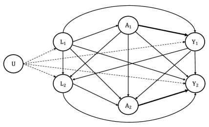
Figure 1: An example causal DAG representing the relationship among confounder, exposure and outcome in time-varying setup.

2.2 G-estimation with repeated outcomes

G-estimation is used for estimating the parameters in SNMMs (Robins and Hernan, , 2008; Vansteelandt and Joffe, , 2014). Under the restriction of stationarity of effects, we can parameterize the blip as a simple function of the history (Vansteelandt and Joffe, , 2014, Section 5.1) that is $\gamma_{j}^{*}(a_{j},\bm{\mathbf{h}}_{ij};\bm{\mathbf{\psi}})=a_{j}\bm{\mathbf{h}}_{ij}^{\top}\bm{\mathbf{\psi}}$, where $\bm{\mathbf{h}}_{ij}$ contains a one and potential confounders chosen from the histories. In this formulation, each component of $\bm{\mathbf{\psi}}$ represents the change in the effect of treatment associated with the corresponding covariate. Under this semiparametric approach, the blip model needs to be correctly specified as a function of the history for consistent estimation of $\bm{\mathbf{\psi}}$. We construct the proximal blipped down outcome as $U_{ij}=Y_{ij}-\gamma_{j}^{*}({A}_{ij},\bm{\mathbf{H}}_{ij};\bm{\mathbf{\psi}})$ at the $j$-th occasion. These blipped down outcomes are a transformation of the observed data such that

$$E[U_{ij}|\bm{\mathbf{H}}_{ij}=\bm{\mathbf{h}}_{ij},A_{ij}=a_{j}]=E[Y_{ij}(\bar{a}_{j-1},0)|\bm{\mathbf{H}}_{ij}=\bm{\mathbf{h}}_{ij},A_{ij}=a_{j}].$$

This implies that the variable $U_{ij}$ has the same mean as the potential outcome under the reference treatment level at occasion $j$. Under the above-mentioned assumptions, the efficient score function (Tsiatis, , 2006) for $\bm{\mathbf{\psi}}$ is given by

$$\bm{\mathbf{S}}^{\text{eff}}(\bm{\mathbf{\psi}}) =\sum_{i=1}^{n}\Big{\{}\frac{\partial\bm{\mathbf{\gamma}}^{*}(\bm{\mathbf{A}}_{i},\bm{\mathbf{H}}_{i};\bm{\mathbf{\psi}})}{\partial\bm{\mathbf{\psi}}^{\top}}-E\Big{(}\frac{\partial\bm{\mathbf{\gamma}}^{*}(\bm{\mathbf{A}}_{i},\bm{\mathbf{H}}_{i};\bm{\mathbf{\psi}})}{\partial\bm{\mathbf{\psi}}^{\top}}|\bm{\mathbf{H}}_{i}\Big{)}\Big{\}}^{\top}\,Var(\bm{\mathbf{U}}_{i}|\bm{\mathbf{H}}_{i})^{-1}\{\bm{\mathbf{U}}_{i}-E(\bm{\mathbf{U}}_{i}|\bm{\mathbf{H}}_{i})\},$$ (2)

where $\bm{\mathbf{A}}_{i}=(A_{i1},\ldots,A_{iJ})^{\top}$, $\bm{\mathbf{H}}_{i}=(\bm{\mathbf{H}}_{i1},\ldots,\bm{\mathbf{H}}_{iJ})^{\top}$ is a $J\times K$ matrix representing the unit-wise history for the $i$-th subject, $\bm{\mathbf{U}}_{i}=(U_{i1},\ldots,U_{iJ})^{\top}$, $E(\bm{\mathbf{U}}_{i}|\bm{\mathbf{H}}_{i})=\bm{\mathbf{H}}_{i}\bm{\mathbf{\delta}}$ is the treatment-free model, and $\bm{\mathbf{\delta}}$ denotes the corresponding parameters.

We define the whole parameter vector as $\bm{\mathbf{\theta}}=(\bm{\mathbf{\delta}}^{\top},\bm{\mathbf{\psi}}^{\top})^{\top}$ and denote the corresponding efficient score function by $\bm{\mathbf{S}}^{\text{eff}}(\bm{\mathbf{\theta}})$ (form is given in the appendix Section A.1). We express the covariance matrix of $\bm{\mathbf{U}}_{i}$ as

$$Var(\bm{\mathbf{U}}_{i}|\bm{\mathbf{H}}_{i})=\bm{\mathbf{Q}}_{i}^{1/2}\,\bm{\mathbf{R}}_{i}(\alpha)\,\bm{\mathbf{Q}}_{i}^{1/2},$$

where $\bm{\mathbf{U}}_{i}=\bm{\mathbf{Y}}_{i}-\bm{\mathbf{A}}_{i}\cdot\bm{\mathbf{H}}_{i}\bm{\mathbf{\psi}}$, $\bm{\mathbf{Q}}_{i}=\sigma^{2}\bm{\mathbf{I}}_{(J)}$ and $\bm{\mathbf{R}}_{i}(\alpha)$ is the $J\times J$ matrix representing the correlations among the blipped down outcomes of a patient and is defined with parameter $\alpha$. The form of $Var(\bm{\mathbf{U}}_{i}|\bm{\mathbf{H}}_{i})$ resembles the working covariance structure used in generalized estimating equations (Liang and Zeger, , 1986). Since $\bm{\mathbf{Q}}_{i}$ and $\bm{\mathbf{R}}_{i}(\alpha)$ are unknown, we replace these quantities in $\bm{\mathbf{S}}^{\text{eff}}(\bm{\mathbf{\theta}})$ by their estimates. We estimate the parameters $\sigma^{2}$ and $\alpha$ using residual based moment method under a working correlation structure. We replace $\bm{\mathbf{R}}_{i}(\alpha)$ by the estimated correlation matrix $\hat{\bm{\mathbf{R}}}$.

We define $\bm{\mathbf{D}}_{ij}=\{\bm{\mathbf{H}}_{ij}^{\top},(A_{ij}-E(A_{ij}|\bm{\mathbf{H}}_{ij}))\cdot\bm{\mathbf{H}}_{ij}^{\top}\}^{\top}$ and $\bm{\mathbf{D}}_{i}=(\bm{\mathbf{D}}_{i1},\ldots,\bm{\mathbf{D}}_{iJ})^{\top}$ of dimension $J\times 2K$ for $i=1,\ldots,n$, $j=1,\ldots,J$. With $Var(\bm{\mathbf{U}}_{i}|\bm{\mathbf{H}}_{i})$ replaced with its estimate, we can write the efficient score as $\bm{\mathbf{S}}^{\text{eff}}(\bm{\mathbf{\theta}})=\sum_{i=1}^{n}\bm{\mathbf{S}}_{i}^{\text{eff}}(\bm{\mathbf{\theta}})$, where the contribution in the efficient score from the $i$-th subject can be expressed as

$$\bm{\mathbf{S}}_{i}^{\text{eff}}(\bm{\mathbf{\theta}})=\bm{\mathbf{D}}_{i}^{\top}\,Var(\bm{\mathbf{U}}_{i}|\bm{\mathbf{H}}_{i})^{-1}\{\bm{\mathbf{U}}_{i}-E(\bm{\mathbf{U}}_{i}|\bm{\mathbf{H}}_{i})\}=\bm{\mathbf{D}}_{i}^{\top}\,\hat{\bm{\mathbf{Q}}}_{i}^{-1/2}\,\hat{\bm{\mathbf{R}}}^{-1}\,\hat{\bm{\mathbf{Q}}}_{i}^{-1/2}\{\bm{\mathbf{U}}_{i}-E(\bm{\mathbf{U}}_{i}|\bm{\mathbf{H}}_{i})\}.$$

The G-estimates $\hat{\bm{\mathbf{\theta}}}_{n}$ are obtained by solving the estimating equations

$$\bm{\mathbf{S}}^{\text{eff}}(\bm{\mathbf{\theta}})=\bm{\mathbf{0}}.$$ (3)

2.3 Proposed method (Penalized G-estimation)

For simultaneous selection of effect modifiers and estimation of the parameters, we propose a penalized efficient score function using a nonconvex smoothly clipped absolute deviation (SCAD) penalty (Fan and Li, , 2001). The SCAD penalty achieves three desirable properties of variable selection: unbiasedness, sparsity, and continuity (Fan and Li, , 2001). Under the assumptions for identifiability of the target parameter $\bm{\mathbf{\psi}}$ given in section 2.1, we propose the following penalized efficient score function

$$\bm{\mathbf{S}}^{P}(\bm{\mathbf{\psi}}) =\sum_{i=1}^{n}\Big{\{}\frac{\partial\bm{\mathbf{\gamma}}^{*}(\bm{\mathbf{A}}_{i},\bm{\mathbf{H}}_{i};\bm{\mathbf{\psi}})}{\partial\bm{\mathbf{\psi}}^{\top}}-E\Big{(}\frac{\partial\bm{\mathbf{\gamma}}^{*}(\bm{\mathbf{A}}_{i},\bm{\mathbf{H}}_{i};\bm{\mathbf{\psi}})}{\partial\bm{\mathbf{\psi}}^{\top}}|\bm{\mathbf{H}}_{i}\Big{)}\Big{\}}^{\top}\,Var(\bm{\mathbf{U}}_{i}|\bm{\mathbf{H}}_{i})^{-1}$$

$${\hskip 166.2212pt}\times\{\bm{\mathbf{U}}_{i}-E(\bm{\mathbf{U}}_{i}|\bm{\mathbf{H}}_{i})\}-n{\bm{\mathbf{q}}}_{\lambda_{n}}(|\bm{\mathbf{\psi}}|)\text{sign}(\bm{\mathbf{\psi}}),$$ (4)

where $\bm{\mathbf{q}}_{\lambda_{n}}(|\bm{\mathbf{\psi}}|)=(0,q_{\lambda_{n}}(|\psi_{1}|),\ldots,q_{\lambda_{n}}(|\psi_{K-1}|))^{\top}$ and $q(.)$ indicates the first-derivative of the SCAD penalty function given by

$$q_{\lambda_{n}}(\psi)=\lambda_{n}\Big{\{}I(\psi\leq\lambda_{n})+\frac{(b\lambda_{n}-\psi)_{+}}{(b-1)\lambda_{n}}I(\psi>\lambda_{n})\Big{\}}$$

for $\psi\geq 0$ and some $b>2$ with $x_{+}=xI(x>0)$. Fan and Li, (2001) suggested to use $b=3.7$. The amount of shrinkage in estimation is determined by the tuning parameter $\lambda_{n}$.

For the whole parameter vector $\bm{\mathbf{\theta}}$, the proposed penalized efficient score function becomes

$$\bm{\mathbf{S}}^{P}(\bm{\mathbf{\theta}})=\bm{\mathbf{S}}^{\text{eff}}(\bm{\mathbf{\theta}})-n{\bm{\mathbf{q}}}_{\lambda_{n}}(|\bm{\mathbf{\theta}}|)\text{sign}(\bm{\mathbf{\theta}}),$$

where ${\bm{\mathbf{q}}}_{\lambda_{n}}(|\bm{\mathbf{\theta}}|)=(\bm{\mathbf{0}}^{\top},{\bm{\mathbf{q}}}_{\lambda_{n}}(|\bm{\mathbf{\psi}}^{\top}|))^{\top}$. The penalized estimates are obtained by solving the following estimating equations:

$$\bm{\mathbf{S}}^{P}(\bm{\mathbf{\theta}})=\bm{\mathbf{0}}.$$ (5)

Note that we do not penalize the parameters $\bm{\mathbf{\delta}}$ of the treatment-free model and the main effect of the treatment ($\psi_{0}$), because our goal is only to identify the effect modifiers.

For solving the penalized efficient estimating equations (5), we use the minorization-maximization (MM) algorithm for nonconvex penalty discussed by Hunter and Li, (2005). We combine the MM algorithm with the iterative procedure of G-estimation. According to the MM algorithm, the penalized G-estimator $\tilde{\bm{\mathbf{\theta}}}$ approximately satisfies

$$S_{m}^{\text{eff}}(\tilde{\bm{\mathbf{\theta}}})-n\,q_{\lambda_{n}}(|\tilde{\theta}_{m}|)\text{sign}(\tilde{\theta}_{m})\frac{|\tilde{\theta}_{m}|}{\epsilon+|\tilde{\theta}_{m}|}=0$$ (6)

for $m=1,\ldots 2K$, where $S_{m}^{\text{eff}}(\tilde{\bm{\mathbf{\theta}}})$ denotes the $m$-th element of $\bm{\mathbf{S}}^{\text{eff}}(\tilde{\bm{\mathbf{\theta}}})$ and $\epsilon$ can be a small number, e.g. $10^{-6}$. If we take a closer look, it is easy to understand that equations (6) are perturbed versions of the original estimating equations (5). For obtaining the penalized G-estimates, the Newton-Raphson type updating formula at the $t$-th iteration directly follows from equation (6) and is given by:

$$\bm{\mathbf{\theta}}^{t+1}=\bm{\mathbf{\theta}}^{t}+\Big{\{}\bm{\mathbf{H}}_{n}(\bm{\mathbf{\theta}}^{t})+n\bm{\mathbf{E}}_{n}(\bm{\mathbf{\theta}}^{t})\Big{\}}^{-1}\Big{(}\bm{\mathbf{S}}^{\text{eff}}(\bm{\mathbf{\theta}}^{t})-n\bm{\mathbf{E}}_{n}(\bm{\mathbf{\theta}}^{t})\bm{\mathbf{\theta}}^{t}\Big{)},$$ (7)

where

$$\bm{\mathbf{H}}_{n}(\bm{\mathbf{\theta}}^{t})=-E\Big{(}\dfrac{\partial\bm{\mathbf{S}}^{\text{eff}}(\bm{\mathbf{\theta}})}{\partial\bm{\mathbf{\theta}}^{\top}}\Big{)}\Big{|}_{\bm{\mathbf{\theta}}=\bm{\mathbf{\theta}}^{t}}=-E\begin{pmatrix}\dfrac{\partial\bm{\mathbf{S}}^{\text{eff}}_{\bm{\mathbf{\delta}}}}{\partial\bm{\mathbf{\delta}}^{\top}}&\dfrac{\partial\bm{\mathbf{S}}^{\text{eff}}_{\bm{\mathbf{\delta}}}}{\partial\bm{\mathbf{\psi}}^{\top}}\\ \dfrac{\partial\bm{\mathbf{S}}^{\text{eff}}_{\bm{\mathbf{\psi}}}}{\partial\bm{\mathbf{\delta}}^{\top}}&\dfrac{\partial\bm{\mathbf{S}}^{\text{eff}}_{\bm{\mathbf{\psi}}}}{\partial\bm{\mathbf{\psi}}^{\top}}\end{pmatrix}_{\bm{\mathbf{\delta}}=\bm{\mathbf{\delta}}^{t},\bm{\mathbf{\psi}}=\bm{\mathbf{\psi}}^{t}}$$ (8)

and

$$\bm{\mathbf{E}}_{n}(\bm{\mathbf{\theta}}^{t})=diag\Bigg{\{}\bm{\mathbf{0}}^{\top},\frac{q_{\lambda_{n}}(|\psi_{1}|)}{\epsilon+|\psi_{1}|},\ldots,\frac{q_{\lambda_{n}}(|\psi_{K-1}|)}{\epsilon+|\psi_{K-1}|}\Bigg{\}}\Bigg{|}_{\bm{\mathbf{\psi}}=\bm{\mathbf{\psi}}^{t}}.$$ (9)

2.4 Tuning parameter selection

The oracle properties of the penalized estimators rely on the proper choice of tuning parameter. Johnson et al., (2008) considered the generalized cross-vaidation (GCV) statistic (Wahba, , 1985) for selecting the tuning parameter in penalized estimating equations. The use of GCV for such selection was suggested by Tibshirani, (1996) and Fan and Li, (2001). However, Wang et al., (2007) showed that tuning parameter selection using GCV causes a nonignorable overfitting effect even if the sample size goes to infinity. Considering the number of covariates $K$ as fixed, Wang et al., (2007) proposed the Bayesian information criterion (BIC) for tuning parameter selection which showed consistency in the identification of the true model. Later, a modification in the BIC criterion was proposed by Wang et al., (2009) in a moderately high-dimensional setup ($K<n$) and by Fan and Tang, (2013) in an ultra-high dimensional setup ($K>>n$). All of these criteria have the following general form

$$\text{measure of model fit}+\tau_{n}\times\text{measure of model complexity},$$ (10)

where $\tau_{n}$ is a positive sequence.

In the context of variable selection for individualized treatment rules, Bian et al., (2023) and Moodie et al., (2023) used doubly robust information criteria for tuning parameter selection. These criteria are similar to the criterion of Fan and Tang, (2013), except that Bian et al., (2023) and Moodie et al., (2023) introduced a weighted measure of model fitting that incorporates overlap weights. To construct the measure of model fitting we follow an approach similar to Wang et al., (2007) and construct the weighted loss function following Moodie et al., (2023). We define the weighted loss function corresponding to the estimating equations (5) as

$$L(\tilde{\bm{\mathbf{\theta}}}_{\lambda_{n}})=\sum_{i=1}^{n}\sum_{j=1}^{J}|\bm{\mathbf{A}}_{ij}-E(\bm{\mathbf{A}}_{ij}|\bm{\mathbf{H}}_{ij})|\times(\bm{\mathbf{Y}}_{ij}-\bm{\mathbf{H}}_{ij}^{\top}\tilde{\bm{\mathbf{\delta}}}_{\lambda_{n}}-\bm{\mathbf{A}}_{ij}\bm{\mathbf{H}}_{ij}^{\top}\tilde{\bm{\mathbf{\psi}}}_{\lambda_{n}})^{2},$$ (11)

where $|\bm{\mathbf{A}}_{ij}-E(\bm{\mathbf{A}}_{ij}|\bm{\mathbf{H}}_{ij})|$ are the overlap weights and $\tilde{\bm{\mathbf{\theta}}}_{\lambda_{n}}$ denotes the penalized estimate obtained under a fixed value of the tuning parameter $\lambda_{n}$. Since the joint distribution of the data under a non-diagonal correlation structure is unknown/undefined, we construct the loss function associated with the estimating equations under an independence assumption. For the penalized estimating equations (5), the measure of model complexity can be defined with the following generalized degrees of freedom (Johnson et al., , 2008)

$$\text{DF}_{\lambda_{n}}=trace\Bigg{[}\Big{\{}\hat{\bm{\mathbf{H}}}_{n}(\tilde{\bm{\mathbf{\theta}}}_{\lambda_{n}})+n\bm{\mathbf{E}}_{n}(\tilde{\bm{\mathbf{\theta}}}_{\lambda_{n}})\Big{\}}^{-1}\hat{\bm{\mathbf{H}}}_{n}(\tilde{\bm{\mathbf{\theta}}}_{\lambda_{n}})\Bigg{]}.$$

In our setup, we propose the following doubly robust information criterion:

$$\text{DRIC}_{\lambda_{n}} =\log\Bigg{(}\frac{L(\tilde{\bm{\mathbf{\theta}}}_{\lambda_{n}})}{n\times J}\Bigg{)}+\tau_{n}\times\dfrac{\text{DF}_{\lambda_{n}}}{n}.$$ (12)

We set $\tau_{n}=\log\{\log(n)\}\log(2K)$, a consideration similar to Fan and Tang, (2013), where $2K$ represents the dimension of $\bm{\mathbf{\theta}}$. Note that we can even consider $\tau_{n}=\log(n)$ in the low dimensional setting.

We compute the DRIC for a sequence of values for $\lambda_{n}$ which are in decreasing order. Typically, the first element ($\lambda_{max}$) in this sequence is the lowest positive number such that all the effect modifiers are eliminated by the method. The last element ($\lambda_{min}$) is a value close to zero for which none of the effect modifiers are eliminated. And we consider around one hundred values in between so that we have a fine grid. The optimal tuning parameter is the value of $\lambda_{n}$ that corresponds to the minimum value of $\text{DRIC}_{\lambda_{n}}$. For a specific correlation structure (corstr), the steps for the whole estimation procedure are summarized in Algorithm 1.

Algorithm 1 Penalized G-estimation algorithm

1:procedure penalizedG($\bm{\mathbf{A}},\bm{\mathbf{H}},\bm{\mathbf{Y}},\lambda$, corstr, $\kappa$)

2:     Compute $E(\bm{\mathbf{A}}_{i}|\bm{\mathbf{H}}_{i})$ for $i=1,\ldots,n$ $\triangleright$ logistic regression on the pooled data

3:     $\bm{\mathbf{\theta}}^{\text{up}}\leftarrow\{\sum_{i=1}^{n}\bm{\mathbf{D}}_{i}^{\top}(\bm{\mathbf{H}}_{i}\;\;\bm{\mathbf{A}}_{i}\cdot\bm{\mathbf{H}}_{i})\}^{-1}\sum_{i=1}^{n}\bm{\mathbf{D}}_{i}^{\top}\bm{\mathbf{Y}}_{i}$ $\triangleright$ univariate unpenalized G-estimator

4:     for all $\lambda\in(\lambda_{max},\ldots,\lambda_{min})$ do

5:         Initialize: $t=0$, $\bm{\mathbf{\theta}}^{0}\leftarrow\bm{\mathbf{\theta}}^{\text{up}}$

6:         repeat

7:              $\bm{\mathbf{e}}_{i}\leftarrow\bm{\mathbf{Y}}_{i}-(\bm{\mathbf{H}}_{i}\;\;\bm{\mathbf{A}}_{i}\cdot\bm{\mathbf{H}}_{i})\bm{\mathbf{\theta}}^{t}$ for $i=1,\ldots,n$

8:              Compute $\sigma^{t}$ and $\alpha^{t}$ under corstr using A.2 $\triangleright$ method of moments estimator

9:              Compute $\hat{\bm{\mathbf{V}}}_{i}$ according to corstr for $i=1,\ldots,n$ $\triangleright$ $\hat{\bm{\mathbf{V}}}_{i}=\hat{\bm{\mathbf{V}}}$ $\forall i$ if $J$ is fixed

10:              Compute $\bm{\mathbf{S}}^{\text{eff}}(\bm{\mathbf{\theta}}^{t})$ using (A.1)

11:              Compute $\bm{\mathbf{H}}_{n}(\bm{\mathbf{\theta}}^{t})$ and $\bm{\mathbf{E}}_{n}(\bm{\mathbf{\theta}}^{t})$ using (8) and (9), respectively.

12:              Update $\bm{\mathbf{\theta}}^{t}$ according to (7) and obtain $\bm{\mathbf{\theta}}^{t+1}$

13:              $t\leftarrow t+1$

14:         until $||\bm{\mathbf{\theta}}^{t}-\bm{\mathbf{\theta}}^{t-1}||<\kappa$$\triangleright$ we set $\kappa=10^{-4}$

15:         $\tilde{\bm{\mathbf{\theta}}}_{\lambda}\leftarrow\bm{\mathbf{\theta}}^{t}$, $\tilde{\sigma}_{\lambda}\leftarrow\sigma^{t}$, and $\tilde{\alpha}_{\lambda}\leftarrow\alpha^{t}$

16:         Compute $\text{DRIC}_{\lambda}$ according to (12)

17:     end for

18:     $\tilde{\bm{\mathbf{\theta}}}\leftarrow\tilde{\bm{\mathbf{\theta}}}_{\lambda}^{*}$ such that $\tilde{\bm{\mathbf{\theta}}}_{\lambda}^{*}$ corresponds to the minimum of $\text{DRIC}_{\lambda}$

19:     return $\tilde{\bm{\mathbf{\theta}}}$

20:end procedure

2.5 Asymptotic properties

In this section, we study the asymptotic properties of the proposed penalized G-estimator where we assume a constant cluster size (i.e. the same number of sessions per patient). Let $\bm{\mathbf{\theta}}_{0}=(\bm{\mathbf{\delta}}_{0}^{\top},\bm{\mathbf{\psi}}^{\top}_{0})^{\top}$ have dimension $2K$, where $\bm{\mathbf{\delta}}_{0}$ is the $K$-dimensional vector of population parameters corresponding to the assumed treatment-free model and $\bm{\mathbf{\psi}}_{0}$ is the $K$-dimensional vector of true coefficients of the blip model. Let $B_{1}=\{1,\ldots,K+1\}$ be the set representing the indices of the unpenalized main effects ($\bm{\mathbf{\delta}}_{0}$ and $\psi_{00}$) and $B_{2}=\{m:\psi_{0m}\neq 0;m=K+2,\ldots,2K\}$ be the index set for the variables that are true effect modifiers of the treatment within this model. Let $B=B_{1}\cup B_{2}$ and $s$ denote the cardinality of the set $B$. Then let $B^{c}$ represent the indices of the zero coefficients in $\bm{\mathbf{\psi}}_{0}$, i.e. the indices of the variables that do not modify the effect of the treatment.

Let $\hat{\bm{\mathbf{R}}}$ introduced in Section 2.2 satisfy $||\hat{\bm{\mathbf{R}}}^{-1}-\overline{\bm{\mathbf{R}}}^{-1}||=O_{p}(\sqrt{1/n})$, where $\overline{\bm{\mathbf{R}}}=E(\hat{\bm{\mathbf{R}}})$ is a constant positive definite matrix with eigenvalues bounded away from zero and $+\infty$. Note that $||\bm{\mathbf{X}}||=\{trace(\bm{\mathbf{X}}\bm{\mathbf{X}}^{\top})\}^{1/2}$ denotes the Frobenius norm of the matrix $\bm{\mathbf{X}}$. Define two versions of the expected information as

$$\bm{\mathbf{H}}(\bm{\mathbf{\theta}}) =E[-\partial\bm{\mathbf{S}}_{i}^{\text{eff}}(\bm{\mathbf{\theta}})/\partial\bm{\mathbf{\theta}}^{\top}]=\bm{\mathbf{D}}_{i}^{\top}\bm{\mathbf{Q}}_{i}^{-1/2}\overline{\bm{\mathbf{R}}}^{-1}\bm{\mathbf{Q}}_{i}^{-1/2}(\bm{\mathbf{H}}_{i}\;\;\bm{\mathbf{A}}_{i}\cdot\bm{\mathbf{H}}_{i}),$$

$$\bm{\mathbf{I}}(\bm{\mathbf{\theta}}) =E[\bm{\mathbf{S}}_{i}^{\text{eff}}(\bm{\mathbf{\theta}})\bm{\mathbf{S}}_{i}^{\text{eff}}(\bm{\mathbf{\theta}})^{\top}]=\bm{\mathbf{D}}_{i}^{\top}\bm{\mathbf{Q}}_{i}^{-1/2}\overline{\bm{\mathbf{R}}}^{-1}\bm{\mathbf{R}}_{0}\overline{\bm{\mathbf{R}}}^{-1}\bm{\mathbf{Q}}_{i}^{-1/2}\bm{\mathbf{D}}_{i},$$

where $\bm{\mathbf{R}}_{0}$ is the true correlation matrix. Details regarding the expressions of these information matrices can be found in Balan and Schiopu-Kratina, (2005), where the authors presented a rigorous asymptotic theory for generalized estimating equations.

According to Johnson et al., (2008), for establishing the asymptotic properties, the required conditions on the efficient score function and the penalty function are as follows:

1. There exists a non-singular matrix $\bm{\mathbf{H}}(\bm{\mathbf{\theta}}_{0})$ such that for any given constant $Z$,

   $$\sup_{|\theta-\theta_{0}|\leq Zn^{-1/2}}|n^{-1/2}\bm{\mathbf{S}}^{\text{eff}}(\theta)-n^{-1/2}\bm{\mathbf{S}}^{\text{eff}}(\theta_{0})-n^{1/2}\bm{\mathbf{H}}(\bm{\mathbf{\theta}}_{0})(\theta-\theta_{0})|=o_{p}(1).$$

   Moreover,

   $$n^{-1/2}\bm{\mathbf{S}}^{\text{eff}}(\bm{\mathbf{\theta}}_{0})\xrightarrow[]{d}N(\bm{\mathbf{0}},\bm{\mathbf{I}}(\bm{\mathbf{\theta}}_{0})).$$

2. The derivative $q_{\lambda_{n}}(\cdot)$ of the penalty function has the following properties:

   1. For nonzero fixed $\theta$, $\lim n^{1/2}q_{\lambda_{n}}(|\theta|)=0$ and $\lim q^{\prime}_{\lambda_{n}}(|\theta|)=0$.

   2. For any $Z>0$, $\lim\sqrt{n}\inf_{|\theta|\leq Zn^{-1/2}}q_{\lambda_{n}}(|\theta|)\rightarrow\infty$,

where $q^{\prime}_{\lambda_{n}}(\cdot)$ denotes the derivative of $q_{\lambda_{n}}(\cdot)$. Under the conditions C.a, C.b and the regularity conditions C1-C7 (provided in Section A.3 in the appendix) applicable for GEE, there exists a root-$n$-consistent approximate zero crossing of $\bm{\mathbf{S}}^{P}(\bm{\mathbf{\theta}})$ indicating $\tilde{\bm{\mathbf{\theta}}}_{n}=\bm{\mathbf{\theta}}_{0}+O_{p}(n^{-1/2})$, such that $\tilde{\bm{\mathbf{\theta}}}_{n}$ is an approximate zero crossing of $\bm{\mathbf{S}}^{P}(\bm{\mathbf{\theta}})$. The proof is analogous to what is presented in Johnson et al., (2008). Also, the proposed estimator enjoys the oracle property, which means that it estimates true zero coefficients as zero with probability approaching one and the true nonzero coefficients as efficiently as if the true model is known in advance. This property is stated in the next two theorems.

Theorem 1

Let $\bm{\mathbf{\theta}}^{B}$ represent the elements of $\bm{\mathbf{\theta}}$ whose indices belong to $B$. Under the required conditions (C.a, C.b and C1-C7), if $\lambda_{n}\rightarrow 0$ and $\sqrt{n}\lambda_{n}\rightarrow\infty$ as $n\rightarrow\infty$, then there exists an approximate penalized G-estimator $\tilde{\bm{\mathbf{\theta}}}_{n}=\{\tilde{\bm{\mathbf{\theta}}}_{n}^{B},\tilde{\bm{\mathbf{\theta}}}_{n}^{B^{c}}\}$ such that

$$P\Big{(}\tilde{\bm{\mathbf{\theta}}}_{n}^{B^{c}}=0\Big{)}\rightarrow 1.$$ (13)

This theorem establishes the correct sparsity of the penalized G-estimator. The proof of Theorem 1 is provided in appendix section A.4.

Theorem 2

Let $\bm{\mathbf{D}}_{i,B}$ represent the elements of the matrix $\bm{\mathbf{D}}_{i}$ that correspond to the coefficients $\bm{\mathbf{\theta}}^{B}$. Under the required conditions (C.a, C.b and C1-C7), if $\lambda_{n}\rightarrow 0$ and $\sqrt{n}\lambda_{n}\rightarrow\infty$ as $n\rightarrow\infty$, the penalized G-estimator $\tilde{\bm{\mathbf{\theta}}}_{n}^{B}$ satisfies:

$$n^{1/2}\Big{\{}\bm{\mathbf{H}}_{B}(\bm{\mathbf{\theta}}_{0})+\bm{\mathbf{W}}_{n}(\bm{\mathbf{\theta}}^{B}_{0})\Big{\}}\Big{[}\tilde{\bm{\mathbf{\theta}}}_{n}^{B}-\bm{\mathbf{\theta}}^{B}_{0}+\Big{\{}\bm{\mathbf{H}}_{B}(\bm{\mathbf{\theta}}_{0})+\bm{\mathbf{W}}_{n}(\bm{\mathbf{\theta}}^{B}_{0})\Big{\}}^{-1}\bm{\mathbf{b}}_{n}\Big{]}\xrightarrow[]{d}N\Big{(}\bm{\mathbf{0}},\bm{\mathbf{I}}_{B}(\bm{\mathbf{\theta}}_{0})\Big{)}.$$

where $\bm{\mathbf{H}}_{B}(\bm{\mathbf{\theta}}_{0})$, $\bm{\mathbf{W}}_{n}(\bm{\mathbf{\theta}}_{0}^{B})$ and $\bm{\mathbf{I}}_{B}(\bm{\mathbf{\theta}}_{0})$ are the $s\times s$ submatrices of $\bm{\mathbf{H}}(\bm{\mathbf{\theta}}_{0})$, $\bm{\mathbf{W}}_{n}(\bm{\mathbf{\theta}}_{0})$ and $\bm{\mathbf{I}}(\bm{\mathbf{\theta}}_{0})$ that correspond to the indices in $B$,

$$\bm{\mathbf{W}}_{n}(\bm{\mathbf{\theta}}_{0})=diag\{\bm{\mathbf{0}}^{\top},-q_{\lambda_{n}}^{\prime}(|\psi_{01}|)\text{sign}(\psi_{01}),\ldots,-q_{\lambda_{n}}^{\prime}(|\psi_{0(K-1)}|)\text{sign}(\psi_{0(K-1)})\},$$

and $\bm{\mathbf{b}}_{n}=-\bm{\mathbf{q}}_{\lambda_{n}}(|\bm{\mathbf{\theta}}_{0}^{B}|)\text{sign}(\bm{\mathbf{\theta}}_{0}^{B})$.

This theorem establishes the asymptotic normality of the penalized G-estimator $\tilde{\bm{\mathbf{\theta}}}_{n}^{B}$. The proof of Theorem 2 is provided in appendix section A.5.

An asymptotic sandwich covariance estimator for $\tilde{\bm{\mathbf{\theta}}}_{n}^{B}$ directly follows from Theorem 2 and is given by

$$\text{Cov}(\tilde{\bm{\mathbf{\theta}}}_{n}^{B})=n^{-1}\Big{\{}\bm{\mathbf{H}}_{B}(\bm{\mathbf{\theta}}_{0})+\bm{\mathbf{W}}_{n}(\bm{\mathbf{\theta}}^{B}_{0})\Big{\}}^{-1}\bm{\mathbf{I}}_{B}(\bm{\mathbf{\theta}}_{0})\Big{\{}\bm{\mathbf{H}}_{B}(\bm{\mathbf{\theta}}_{0})+\bm{\mathbf{W}}_{n}(\bm{\mathbf{\theta}}^{B}_{0})\Big{\}}^{-1}.$$ (14)

We can consistently estimate the variance in (14) by replacing the quantities in it by their empirical estimates as follows

$$\widehat{\text{Cov}}(\tilde{\bm{\mathbf{\theta}}}_{n}^{B})=n^{-1}\Big{\{}\widehat{\bm{\mathbf{H}}}_{B}(\tilde{\bm{\mathbf{\theta}}}_{n})+\bm{\mathbf{W}}_{n}(\tilde{\bm{\mathbf{\theta}}}_{n}^{B})\Big{\}}^{-1}\widehat{\bm{\mathbf{I}}}_{B}(\tilde{\bm{\mathbf{\theta}}}_{n})\Big{\{}\widehat{\bm{\mathbf{H}}}_{B}(\tilde{\bm{\mathbf{\theta}}}_{n})+\bm{\mathbf{W}}_{n}(\tilde{\bm{\mathbf{\theta}}}_{n}^{B})\Big{\}}^{-1}$$

where $\widehat{\bm{\mathbf{I}}}_{B}(\tilde{\bm{\mathbf{\theta}}}_{n})=n^{-1}\sum_{i=1}^{n}\bm{\mathbf{S}}_{i}^{\text{eff}}(\tilde{\bm{\mathbf{\theta}}}_{n}^{B})\Big{\{}\bm{\mathbf{S}}_{i}^{\text{eff}}(\tilde{\bm{\mathbf{\theta}}}_{n}^{B})\Big{\}}^{\top}$ and $\widehat{\bm{\mathbf{H}}}_{B}(\tilde{\bm{\mathbf{\theta}}}_{n})=-n^{-1}\sum_{i=1}^{n}\dfrac{\partial S_{i}^{\text{eff}}(\bm{\mathbf{\theta}})}{\partial\bm{\mathbf{\theta}}^{\top}}\Big{|}_{\bm{\mathbf{\theta}}=\tilde{\bm{\mathbf{\theta}}}_{n}^{B}}$. Note that Theorem 2 requires the treatment model parameters to be known. Because we estimate the treatment model and use the predicted values in the design matrix for the outcome regression, we need to account for the uncertainty involved in the estimation of the treatment model. So, $\widehat{\bm{\mathbf{I}}}(\tilde{\bm{\mathbf{\psi}}}_{n})$, a submatrix of $\widehat{\bm{\mathbf{I}}}_{B}(\tilde{\bm{\mathbf{\theta}}}_{n})$, should be calculated accounting for that uncertainty as shown in the Appendix Section A.6.

3 Simulation study

In order to evaluate the performance of the proposed estimator in finite samples we conducted two simulation studies. The first evaluates the oracle property mentioned in Theorem 1 and Theorem 2; the setup and results are presented in Section 3.1. The second simulation study in Section 3.2 verifies the double robustness property of our estimator.

3.1 Evaluation of the oracle property in finite samples

To generate the data for $j$-th session ($j=1,\ldots,J$) of each subject, we generated two baseline confounders as $L^{(1)}\sim Bernoulli(0.5)$ and $L^{(2)}\sim N(0,1)$, and the time varying confounders and noise covariates as $L_{j}^{(3)},\ldots,L_{j}^{(6)},X_{j}^{(1)},\ldots,X_{j}^{(10)}\sim MVN_{14}\Big{(}(\bm{\mathbf{\mu}}_{L,j}^{\top},\bm{\mathbf{\mu}}_{X,j}^{\top})^{\top},\bm{\mathbf{V}}\Big{)}$, where $\mu_{L,j}^{(k)}=0.3\,l^{(k)}_{j-1}+0.3\,a_{j-1}$ for $k=3,4,5\text{ and }6$, and $\mu_{X,j}^{(r)}=0.5\,x^{(r)}_{j-1}$ for $r=1,\ldots,10$. Note that we define $l_{0}^{(k)}=0$ for any $k$, $a_{0}=0$, and $x_{0}^{(r)}=0$ for any $r$. The covariance matrix $\bm{\mathbf{V}}$ has $(r,s)$-th element equal to $\rho^{|r-s|}$ for $r,s=1,\ldots,14$. We generated the binary exposure according to the probability

$$P(A_{j}=1|\bm{\mathbf{H}}_{j})=\dfrac{\exp{(\beta_{0}+\beta_{1}l^{(1)}+\beta_{2}l^{(2)}+\sum_{m=3}^{6}\beta_{m}l_{j}^{(m)}+\beta_{7}a_{j-1})}}{1+\exp{(\beta_{0}+\beta_{1}l^{(1)}+\beta_{2}l^{(2)}+\sum_{m=3}^{6}\beta_{m}l_{j}^{(m)}+\beta_{7}a_{j-1})}}.$$ (15)

We then generated a vector of correlated errors $\bm{\mathbf{\epsilon}}\sim N_{J}(\bm{\mathbf{0}},\bm{\mathbf{\Sigma}})$, where $\bm{\mathbf{\Sigma}}=\sigma^{2}_{\epsilon}\bm{\mathbf{R}}$ is the variance-covariance matrix and $\bm{\mathbf{R}}$ is the $J\times J$ correlation matrix defined with parameter $\alpha$ according to a “exchangeable” correlation structure. Finally, we constructed the outcome as

$$y_{j}=\mu_{j}(\bm{\mathbf{h}}_{j};\bm{\mathbf{\delta}})+\gamma^{*}_{j}(a_{j},\bm{\mathbf{h}}_{j};\bm{\mathbf{\psi}})+\epsilon_{j},$$

where $\mu_{j}(\bm{\mathbf{h}}_{j};\bm{\mathbf{\delta}})=\delta_{0}+\delta_{1}l^{(1)}+\delta_{2}l^{(2)}+\sum_{m=3}^{6}\delta_{m}l_{j}^{(m)}+\delta_{7}\exp(l_{j}^{(5)})+\delta_{8}a_{j-1}$ and $\gamma^{*}_{j}(a_{j},\bm{\mathbf{h}}_{j};\bm{\mathbf{\psi}})=(\psi_{0}+\psi_{1}l^{(1)}+\psi_{2}l^{(2)}+\sum_{m=3}^{6}\psi_{m}l_{j}^{(m)}+\psi_{7}a_{j-1})a_{j}$. Let $\bm{\mathbf{\beta}}=(\beta_{0},\ldots,\beta_{7})^{\top}$, $\bm{\mathbf{\delta}}=(\delta_{0},\ldots,\delta_{8})^{\top}$ and $\bm{\mathbf{\psi}}=(\psi_{0},\ldots,\psi_{7})^{\top}$. We fixed $\bm{\mathbf{\beta}}=(0,1,1,1,1,1,1,-0.8)^{\top}$, $\bm{\mathbf{\delta}}=(1,-1,1,1,1,1,1,1,1)^{\top}$ and we considered two different models for the blip;

• Setting 1 (stronger effect modification): $\bm{\mathbf{\psi}}=(1,-2.5,1.5,1.5,1.5,1.5,0,2)^{\top}$

• Setting 2 (weaker effect modification): $\bm{\mathbf{\psi}}=(1,-2,1,0.75,0.9,1.2,0,1.8)^{\top}$.

Note that none of the $X$’s were used to generate $\mu_{j}(\bm{\mathbf{h}}_{j};\bm{\mathbf{\delta}})$ and $\gamma^{*}_{j}(a_{j},\bm{\mathbf{h}}_{j};\bm{\mathbf{\psi}})$. We considered $n=200$, $\rho=0$ vs. 0.25, $\sigma^{2}_{\epsilon}=1$ vs. 4 and $\alpha=0.8$. All of the confounders and noise covariates were considered candidates for effect modification. We performed the proposed penalized G-estimation using three different working correlation structures: independent (Indep), exchangeable (Exch), and unstructured (UN). In all the scenarios, we compare the estimates under a misspecified treatment-free model. We consider a variable to be eliminated by the method if $|\text{effect modification}|<0.001$. For evaluating the model selection performance, we considered the rate of false negatives (FN) (i.e. the proportion of times the method eliminated at least one true effect modifier), the rate of false positives (FP) (i.e. the proportion of times the method select at least one covariate which is not a true effect modifier), and the rate of exact selections (EXACT) (i.e. proportion of times the method selected the true set of effect modifiers). We also reported the average number of false positives (AFP), i.e. the average number of variables selected by the method which do not belong to the set of true effect modifiers. The performance measures for different settings were calculated from 500 independent simulations and are shown in Table 1.

Table 1: Model selection performance of the penalized G-estimator for data generated with $n=200$, $J=6$ for all $i$, an exchangeable correlation structure and $\alpha=0.8$ under varying values of the error variance $\sigma^{2}_{\epsilon}$ and varying degrees of autocorrelation between the effect modifiers and noise covariates. Results are obtained with a misspecified treatment-free model from 500 independent simulations for Setting 1 and Setting 2.

Autocorr	Working	Setting 1 (Stronger EM)					Setting 2 (Weaker EM)
coeff ($\rho$)	correlation	FN	FP	EXACT	AFP		FN	FP	EXACT	AFP
		$\sigma^{2}_{\epsilon}=1$					$\sigma^{2}_{\epsilon}=1$
	Indep	2.0	1.4	96.6	0.01		9.2	3.6	87.8	0.04
0	Exch	1.6	1.4	97.0	0.01		8.8	2.8	88.8	0.03
	UN	1.4	1.8	96.8	0.02		10.0	2.6	87.4	0.03
	Indep	2.2	6.0	91.8	0.07		3.6	6.6	90.2	0.07
0.25	Exch	1.6	5.6	92.8	0.06		2.4	5.8	92.2	0.06
	UN	1.0	4.8	94.2	0.06		2.0	3.8	94.4	0.04
		$\sigma^{2}_{\epsilon}=4$					$\sigma^{2}_{\epsilon}=4$
	Indep	14.8	2.4	83.0	0.02		44.6	1.4	54.0	0.02
0	Exch	14.2	1.0	84.8	0.01		42.4	0.4	57.2	0.00
	UN	14.6	0.0	85.4	0.00		45.8	0.2	54.2	0.00
	Indep	11.8	3.8	84.4	0.04		28.2	3.4	69.0	0.03
0.25	Exch	10.6	0.6	88.8	0.01		25.4	1.6	73.2	0.02
	UN	9.4	0.6	90.0	0.01		24.8	1.6	74.0	0.02

FN: % of false negatives, FP: % of false positives, EXACT: % of exact selections,
AFP: average false positives, EM: effect modifier,
Indep: independent, Exch: exchangeable, UN: unstructured

The selection rates of the exact model are above 90% for most cases when the error variance is one. When the error variance was increased, the exact selection rate decreased and the false negative rate increased. When the outcomes were more highly correlated and the candidate variables were auto-correlated among themselves, accounting for correlation among the observed outcomes within a patient produced a clear advantage over the independence assumption. In this case, the false negative and false positive rates produced by the working independent structure are higher than the other two structures.

Simulations were also conducted for a larger value of $n$ (=500) with two different values for the correlation parameter $\alpha$ (=0.4 and 0.8) indicating low and high correlation among the repeated outcomes; the results are presented in Table 2. Under the larger sample size ($n=500$) with all other parameters being the same, we see an improved performance of the proposed method (compare the second row of Table 1 to the bottom row of Table 2), supporting the result of Theorem 1.

While generating data, we also considered alternative choices for the exposure model, for example, when the exposure selection probability depends on past outcome (i.e. $Y_{j-1}\rightarrow A_{j}$); the results are provided in Table S1 in the supplementary material. Simulations were also performed under the data generating structure where past outcomes affect future outcomes (i.e. $Y_{j-1}\rightarrow Y_{j}$); the results are provided in Table S2 in the supplementary material. Under these two setups, the selection rates of the true effect modifiers were good when we considered a larger sample size, specifically for the setting with weaker effect modification.

Table 2: Model selection performance of the penalized G-estimator for data generated with $n=500$, $J=6$ for all $i$, an exchangeable correlation structure among the repeated outcomes with varying value of correlation parameter $\alpha$, an autocorrelation coefficient $\rho=0.25$ deciding the correlation among the EM’s and noise covariates, and error variance $\sigma^{2}_{\epsilon}=1$. Results are obtained with a misspecified treatment-free model from 500 independent simulations for Setting 1 and Setting 2.

	Working	Setting 1 (Stronger EM)					Setting 2 (Weaker EM)
$\alpha$	correlation	FN	FP	EXACT	AFP		FN	FP	EXACT	AFP
	Indep	0.4	7.2	92.4	0.08		0.0	5.4	94.6	0.05
0.4	Exch	0.4	7.2	92.4	0.08		0.0	5.8	94.2	0.06
	UN	0.4	5.6	94.0	0.06		0.0	4.6	95.4	0.05
	Indep	0.0	5.8	94.2	0.06		0.2	8.8	91.0	0.09
0.8	Exch	0.0	5.2	94.8	0.06		0.2	6.6	93.2	0.07
	UN	0.0	4.6	95.4	0.05		0.0	6.4	93.6	0.07

FN: % of false negatives, FP: % of false positives, EXACT: % of exact selections,
AFP: average false positives, EM: effect modifier,
Indep: independent, Exch: exchangeable, UN: unstructured

We also compared the performance of the penalized estimator with the Oracle estimator (estimator obtained from the true blip model but with the same misspecification in the treatment-free part) under each of the working correlation structures. In Table 5, we reported the relative bias ($=100\times(\tilde{\psi}_{n}-\psi_{0})/\psi_{0}$), the empirical root-mean-squared error, SE1, and the square root of the average of sandwich variance estimates, SE2, under different working correlation structures. From the results, we see that the usage of non-independent correlation structures resulted in more efficient estimation of the blip parameters. Moreover, the efficiency of the penalized estimates is comparable to that of the oracle estimates, which also verifies the property stated in Theorem 2.

3.2 Verification of the double robustness property

The double robustness of the proposed penalized G-estimator was verified via a simulation experiment with $n=500$ and $J=6$ for all subjects. We considered estimation under four different scenarios: Scenario 1: The treatment model is correct, and the treatment-free model is misspecified, Scenario 2: The treatment model is incorrect, and the treatment-free model is correct, Scenario 3: Both models are correct, and Scenario 4: Both models are misspecified. For data generation, we set $\bm{\mathbf{\beta}}=(0,1,1,1,1,1,1,-0.8)^{\top}$, $\bm{\mathbf{\delta}}=(1,-1,1,1,1,1,1,-0.8,1)^{\top}$, and $\bm{\mathbf{\psi}}=(1,-2.5,1.5,1.5,1.5,1.5,0,2)^{\top}$. This parameter setup was chosen because, with this setup under Scenario 4, where both models are misspecified, the coefficient estimate of at least one true effect modifier was estimated to be around zero. This lets us verify the double robustness property of the proposed estimator in terms of effect modifier selection consistency. Data were generated under an exchangeable structure with $\alpha=0.8$, error variance $\sigma^{2}_{\epsilon}=1$ and autocorrelation coefficient $\rho=0.25$. For each generated data set, we performed the proposed estimation under each of the four scenarios and three working correlation structures. For estimation under Scenario 1, we estimated the propensity score using the true exposure model but excluded the $\exp(L^{(5)})$ predictor from the treatment-free model. In Scenario 2, we included the $\exp(L^{(5)})$ predictor in the treatment-free model but used a null model for estimating the propensity score, i.e., we assigned the overall empirical proportion of exposure as the probability of being exposed at each measurement occasion. In Scenario 3, we estimated the propensity score using the true exposure model and also included $\exp(L^{(5)})$ as a covariate in the treatment-free model. Finally, in Scenario 4, we considered a null model for estimating the propensity score and also excluded $\exp(L^{(5)})$ as a covariate in the treatment-free part. We report the percentage selection for each of the candidate effect modifiers with rates of false negative, false positive, and exact selection in Table 3.

Table 3: Variable selection rates (%) from the penalized G-estimation under different scenarios with different working correlation structures. Data were generated with $n=500$, $J=6$ for all $i$, an exchangeable correlation structure with $\alpha=0.8$, error variance $\sigma^{2}_{\epsilon}=1$ and autocorrelation coefficient $\rho=0.25$ inducing correlation among the effect modifiers and noise covariates. Results are obtained from 500 independent simulations.

	Scenario 1				Scenario 2				Scenario 3				Scenario 4
	Indep	Exch	UN		Indep	Exch	UN		Indep	Exch	UN		Indep	Exch	UN
$A\times L^{(1)}$	100	100	100		100	100	100		100	100	100		100	100	100
$A\times L^{(2)}$	100	100	100		100	100	100		100	100	100		100	100	100
$A\times L^{(3)}$	100	100	100		100	100	100		100	100	100		100	100	100
$A\times L^{(4)}$	100	100	100		100	100	100		100	100	100		100	100	100
$A\times L^{(5)}$	100	100	100		100	100	100		100	100	100		6.6	7.0	8.2
$A\times L^{(6)}$	5.8	4.4	3.6		0.0	0.0	0.0		2.2	0.0	0.0		0.2	0.0	0.0
$A\times\exp{(L^{(5)})}$	-	-	-		0.0	0.6	0.4		3.2	0.0	0.0		-	-	-
$A\times A_{\text{Lag1}}$	100	100	100		100	100	100		100	100	100		100	100	100
$A\times X^{(1)}$	0.0	0.2	0.2		0.2	0.0	0.0		2.0	0.0	0.0		0.2	0.0	0.0
$A\times X^{(2)}$	0.4	0.2	0.0		0.0	0.0	0.0		1.2	0.0	0.0		0.0	0.0	0.0
$A\times X^{(3)}$	0.2	0.4	0.4		0.2	0.0	0.0		2.2	0.0	0.0		0.2	0.0	0.0
$A\times X^{(4)}$	0.2	0.2	0.2		0.0	0.0	0.0		2.8	0.0	0.0		0.4	0.0	0.0
$A\times X^{(5)}$	0.0	0.2	0.4		0.0	0.0	0.0		1.6	0.0	0.0		0.0	0.0	0.0
$A\times X^{(6)}$	0.0	0.2	0.4		0.0	0.0	0.0		2.2	0.0	0.0		0.0	0.0	0.0
$A\times X^{(7)}$	0.0	0.0	0.0		0.0	0.0	0.0		2.2	0.0	0.0		0.0	0.0	0.0
$A\times X^{(8)}$	0.4	0.4	0.4		0.2	0.0	0.0		2.6	0.0	0.0		0.0	0.0	0.0
$A\times X^{(9)}$	0.0	0.0	0.2		0.0	0.0	0.0		3.0	0.0	0.0		0.2	0.0	0.0
$A\times X^{(10)}$	0.2	0.2	0.8		0.2	0.0	0.0		2.8	0.0	0.0		0.0	0.0	0.0
FN	0.0	0.0	0.0		0.0	0.0	0.0		0.0	0.0	0.0		93.4	93.0	91.8
FP	6.8	6.0	5.8		0.6	0.6	0.4		20.6	0.0	0.0		1.0	0.0	0.0
EXACT	93.2	94.0	94.2		99.4	99.4	99.6		79.4	100	100		6.2	7.0	8.2

FN: % of false negatives, FP: % of false positives, EXACT: % of exact selections,
AFP: average false positives, EM: effect modifier,
Indep: independent, Exch: exchangeable, UN: unstructured
Scenario 1: treatment model correct, Scenario 2: treatment-free model correct,
Scenario 3: both correct, Scenario 4: both incorrect

When both the treatment and the treatment-free models were incorrect (Scenario 4), the proposed method did not select the true effect modifier, $L^{(5)}$, in more than 70% of the simulations irrespective of what the correlation structure was. Misspecification of the functional form of this effect modifier in the treatment-free part caused a biased estimation of its coefficient in the blip model. The direction of this bias was towards the null, and as a result, we observed the exclusion of this effect modifier in the majority of the simulations. But when at least one of those models was correct (Scenarios 1 to 3) the proposed method performed will in identifying the true effect modifiers under the non-independent correlation structures. When both models were correct (Scenario 3), the false positive rates were higher under the independent structure when compared with exchangeable and unstructured correlation structures.

4 Analyzing effect heterogeneity of the dialysis facility on the hemodiafiltration outcome

Our study data arise from an open cohort of patients undergoing chronic hemodiafiltration at the University of Montreal Hospital Centre (CHUM) outpatient dialysis clinic or its affiliated ambulatory dialysis center (CED). Hemodiafiltration was considered as chronic if there were least 28 consecutive sessions. The cohort start-date for each patient was their first dialysis session on or after March 1st, 2017; the cohort end date was December 1st, 2021. The primary data include information from a total of 474 patients who underwent 170761 dialysis sessions. The following information was extracted from hospital databases for each session: drugs (BDM), laboratory results (CERNER), procedures related to dialysis venous access (Radimage), and dialysis-related variables and dialysis-related drugs (EuCliD-NephroCare). EuCliD includes longitudinal and quasi real-time data automatically recorded via electronic upload or manually collected by the clinical staff. We received the cleaned study dataset comprised of time-varying elements of the hemodiafiltration prescription predicting convection volume, concomitant therapies to manage anemia or low albumin or to maintain dialysis access patency, and dialysis session-specific results. Comorbidities that are potential confounders were obtained from the Maintenance et exploitation des données pour l’étude de la clientèle hospitalière (MED-ECHO) database. Confounders and potential effect modifiers that we considered in the analysis are previous outcome (24L or less$=1$ vs. more than 24L $=0$), hemoglobin, albumin, dalteparin, access (fistula = 0, catheter = 1), catheter change, age, sex (male = 1, female = 0), and the components of the Charlson Comorbidity Index (hypertension, diabetes, peripheral vascular disease, congestive heart failure, cardiac arrhythmia, acute myocardial infarction, chronic pulmonary disease, liver disease, valvular disease, cancer, metastatic cancer, cerebrovascular disease, dementia, hemiplegia, and rheumatic disease). The exposure is the dialysis facility and coded as one if the treatment location was CHUM and zero if the location was CED.

The primary data is comprised of information from all dialysis sessions of the patients during the study period (March 1st, 2017 to December 1st, 2021). The inclusion of all of these sessions neither falls under the scope of the proposed method nor is relevant to answering the research question of interest. Being guided by the subject matter expert, we included the first six consecutive sessions of post-dilution hemodiafiltration for each of the patients in our analysis. We estimated the propensity scores using a logistic regression of exposure conditional on all of the potential confounders using the pooled data set. Next we performed the proposed penalized G-estimation considering four different correlation structures (independent, exchangeable, autoregressive of order one or AR1 and unstructured). For $j$-th session, for example, under the AR1 correlation structure, the selected blip model (with adjustment for all potential confounders in the treatment-free part) is

$$\small\gamma_{j}(a_{j},\bm{\mathbf{h}}_{j};\bm{\mathbf{\psi}})=(\psi_{0}+\psi_{1}\times\text{Cancer}_{j})\,\text{Location\_CHUM}_{j}$$

for $j=1,2,\ldots,6$. The estimates of the blip parameters are given in Table 4 with their corresponding sandwich standard error estimates.

Table 4: Estimated blip parameters and corresponding standard errors under different working correlation structures for the hemodiafiltration study.

	Indep			Exch			AR1			UN
	Est	SE		Est	SE		Est	SE		Est	SE
location_CHUM	-0.83	0.24		-1.51	0.32		-1.85	0.31		-1.71	0.34
location_CHUM$\times$cancer	-	-		-	-		3.89	0.78		3.37	0.75

The sign of the estimated main effect of the exposure is negative under each of the working correlation structures considered. Under the AR1 and unstructured correlation structures, cancer was selected by the method, indicating that the effect of dialysis facility on the convection volume differs by the cancer status of the patient. If we interpret the results obtained under the AR1 correlation structure we can say that among the patients who did not have cancer the mean convection volume was 1.85 litres lower at CHUM when compared with CED at fixed levels of all other confounders. But, the mean convection volume was $3.89-1.85=2.04$ litres higher at the CHUM for cancer patients indicating that cancer patients with same measurements on the adjusted confounders had better hemodiafiltration outcomes at the CHUM. However, it is important to note that the final model was determined by data-driven variable selection. So confidence intervals based on the sandwich standard error estimates may produce invalid inference with inflated type I error. In this article, we provided the standard error estimates to have an approximate idea of the amount of sampling error in the estimates.

5 Discussion

In this study, we proposed penalizing the estimating equations of G-estimation for evaluating the causal effect of a time-varying exposure with automatic effect modifier selection with longitudinal observational data and a proximal outcome of interest. We applied this method to investigate if the effect of dialysis facility on the dialysis outcome (convection volume) differs by the demographic and clinical characteristics and comorbidity status of the patients with end-stage renal disease. Our findings suggest that the effect of dialysis facility on the convection volume might differ by the cancer status of the patient. Cancer patients of CHUM had better hemodiafiltration outcomes than the cancer patients dialyzed at CED, given that the two groups were similar in terms of other measured characteristics.

For consistent estimation of the target (blip) parameters with our method, at least one of the treatment-free model and the treatment model needs to be correctly specified. Although we did not perform variable selection for the treatment model in our application concerning the hemodiafiltarion study, such selection may be necessary, in practice, especially in a high-dimensional setup. Methods are available in the literature to accomplish this task, for example, see the work by Shortreed and Ertefaie, (2017). We used the SCAD penalty for penalizing the estimating equations. An alternative choice could be the adaptive Least Absolute Shrinkage and Selection Operator (adaptive LASSO) penalty proposed by Zou, (2006). For selecting the tuning parameter, we considered a doubly robust information criterion (DRIC). Wang et al., (2012) used cross-validation for selecting the tuning parameter in a penalized generalized estimating equation, minimizing the prediction error under an independence assumption. We followed a similar idea and constructed the loss function in the DRIC using an independent correlation structure. Although we considered a repeated outcomes setup, in our study, we did not consider the quasi information criterion (QIC) (Pan, , 2001), which extends the AIC in the longitudinal setup. Because the QIC might experience similar overfitting issues as the AIC and since our goal is to select the true effect modifiers in SNMMs, we instead used a doubly robust information criterion for tuning parameter selection in the proposed penalized G-estimation.

In our simulation study, our method performed well in selecting the true blip model from a set of candidate models, even when we assumed no correlation between the outcomes from the same patient. However, when we used the correct correlation structure, the method produced better estimates of the target (blip) parameters than a working independent model. The efficiency of the penalized estimates was comparable to that of the oracle estimates of the blip parameters. Although we considered different non-independent correlation structures in the simulation studies and in the data application, it is possible to choose an appropriate correlation structure using the data (Jaman et al., , 2016; Inan et al., , 2019; Sultana et al., , 2023). The selection rates of the true blip model were good in the majority of our simulation scenarios. However, these rates depend on the magnitude of effect modification and the signal to noise ratio. A challenge still remains in the identification of weak effect modifiers and this would be an interesting topic for future research. Researchers may wish to study the article by Gunter et al., (2011), where the authors discussed a ranking procedure for selecting effect modifiers that are weaker but important for decision making.

Future work can consider extension of this work for estimation of delayed effects of past exposure. Another topic of interest is developing methods for consistent estimation of the blip parameters when the blip model is misspecified or an effect modifier is unmeasured, for example, see the work by Boruvka et al., (2018). The development of post-selection inference for the proposed estimator opens up another potential branch of research.

Acknowledgements
This work is supported by a doctoral scholarship from the Fonds de Recherche du Québec Nature et technologies (FRQNT) of Canada to AJ and a Discovery Grant from the Natural Sciences and Engineering Research Council of Canada to MES. AE is supported by the research grants (R01DA048764 and R33NS120240) from the National Institutes of Health. MES is supported by a tier 2 Canada Research Chair. We acknowledge Professor Erica E.M. Moodie (McGill University) for her guidance on tuning parameter selection.

Table 5: Relative bias (%), empirical (SE1) and sandwich (SE2) estimates of the standard errors for the penalized and the oracle estimators calculated from 500 simulations for $n=500$, autocorrelation coefficient $\rho=0.25$, error variance $\sigma_{\epsilon}^{2}=1$, and $\alpha=0.8$ under the two settings.

Working		Penalized								Oracle
model	Stats	$\psi_{0}$	$\psi_{1}$	$\psi_{2}$	$\psi_{3}$	$\psi_{4}$	$\psi_{5}$	$\psi_{7}$		$\psi_{0}$	$\psi_{1}$	$\psi_{2}$	$\psi_{3}$	$\psi_{4}$	$\psi_{5}$	$\psi_{7}$
Setting 1
(Stronger EM)
Ind	r.bias	1.32	-1.04	0.05	0.00	0.40	0.06	0.21		1.37	-0.94	0.13	0.18	0.23	0.11	0.04
Ind	SE1	0.16	0.19	0.11	0.11	0.11	0.18	0.19		0.16	0.19	0.11	0.11	0.11	0.18	0.19
Ind	SE2	0.16	0.19	0.11	0.10	0.11	0.18	0.20		0.16	0.19	0.11	0.10	0.11	0.18	0.20
Exch	r.bias	1.13	-1.11	0.01	0.06	0.44	1.30	0.24		1.17	-1.03	0.16	0.21	0.30	1.35	0.03
Exch	SE1	0.14	0.18	0.10	0.10	0.10	0.17	0.17		0.14	0.18	0.10	0.10	0.10	0.17	0.17
Exch	SE2	0.14	0.18	0.10	0.10	0.10	0.17	0.18		0.14	0.18	0.10	0.10	0.10	0.17	0.18
UN	r.bias	1.00	-1.02	0.05	0.01	0.47	1.76	0.10		1.02	-0.95	0.17	0.11	0.35	1.80	0.07
UN	SE1	0.15	0.19	0.11	0.10	0.10	0.17	0.18		0.15	0.19	0.11	0.10	0.10	0.17	0.18
UN	SE2	0.14	0.18	0.10	0.10	0.10	0.17	0.19		0.14	0.18	0.10	0.10	0.10	0.17	0.19
Setting 2
(Weaker EM)
Ind	r.bias	0.53	-1.01	0.84	1.97	1.59	0.23	2.23		0.47	-0.78	0.44	1.40	1.10	0.31	1.80
Ind	SE1	0.15	0.20	0.11	0.11	0.11	0.19	0.21		0.15	0.20	0.11	0.11	0.11	0.19	0.21
Ind	SE2	0.16	0.19	0.11	0.11	0.11	0.18	0.20		0.16	0.19	0.11	0.11	0.11	0.18	0.20
Exch	r.bias	0.19	-1.09	0.69	1.69	1.17	1.58	1.76		0.15	-0.94	0.39	1.30	0.81	1.62	1.44
Exch	SE1	0.14	0.19	0.11	0.10	0.11	0.18	0.19		0.14	0.19	0.11	0.10	0.10	0.18	0.19
Exch	SE2	0.14	0.18	0.10	0.10	0.10	0.17	0.18		0.14	0.18	0.10	0.10	0.10	0.17	0.18
UN	r.bias	0.61	-0.93	0.85	1.46	1.13	2.28	1.82		0.57	-0.76	0.53	1.04	0.75	2.38	1.49
UN	SE1	0.14	0.20	0.11	0.10	0.11	0.18	0.20		0.14	0.20	0.11	0.10	0.11	0.18	0.20
UN	SE2	0.14	0.18	0.10	0.10	0.10	0.17	0.19		0.14	0.18	0.10	0.10	0.10	0.17	0.19

r.bias $=100\times(\tilde{\theta}_{n}-\theta_{0})/\theta_{0}$); SE1: the empirical root-mean squared error (MSE);
SE2: the square-root of the average of sandwich variance estimates

Appendix A Appendix

A.1 Form of efficient score

The efficient score vector is $\bm{\mathbf{S}}^{\text{eff}}(\bm{\mathbf{\theta}})=[\bm{\mathbf{S}}^{\text{eff}}(\bm{\mathbf{\delta}})^{\top},\bm{\mathbf{S}}^{\text{eff}}(\bm{\mathbf{\psi}})^{\top}]^{\top}$, where

$$\bm{\mathbf{S}}^{\text{eff}}(\bm{\mathbf{\delta}}) =\sum_{i=1}^{n}\Big{\{}\frac{\partial\bm{\mathbf{\mu}}(\bm{\mathbf{H}}_{i};\bm{\mathbf{\delta}})}{\partial\bm{\mathbf{\delta}}^{\top}}\Big{\}}^{\top}\,Var(\bm{\mathbf{U}}_{i}|\bm{\mathbf{H}}_{i})^{-1}\{\bm{\mathbf{U}}_{i}-E(\bm{\mathbf{U}}_{i}|\bm{\mathbf{H}}_{i})\}$$

$$=\sum_{i=1}^{n}\bm{\mathbf{H}}_{i}^{\top}\,Var(\bm{\mathbf{U}}_{i}|\bm{\mathbf{H}}_{i})^{-1}\{\bm{\mathbf{U}}_{i}-E(\bm{\mathbf{U}}_{i}|\bm{\mathbf{H}}_{i})\}$$

$$\bm{\mathbf{S}}^{\text{eff}}(\bm{\mathbf{\psi}}) =\sum_{i=1}^{n}\Big{\{}\frac{\partial\bm{\mathbf{\gamma}}^{*}(\bm{\mathbf{A}}_{i},\bm{\mathbf{H}}_{i};\bm{\mathbf{\psi}})}{\partial\bm{\mathbf{\psi}}^{\top}}-E\Big{(}\frac{\partial\bm{\mathbf{\gamma}}^{*}(\bm{\mathbf{A}}_{i},\bm{\mathbf{H}}_{i};\bm{\mathbf{\psi}})}{\partial\bm{\mathbf{\psi}}^{\top}}|\bm{\mathbf{H}}_{i}\Big{)}\Big{\}}^{\top}\,Var(\bm{\mathbf{U}}_{i}|\bm{\mathbf{H}}_{i})^{-1}\{\bm{\mathbf{U}}_{i}-E(\bm{\mathbf{U}}_{i}|\bm{\mathbf{H}}_{i})\}$$

$$=\sum_{i=1}^{n}\Big{\{}(\bm{\mathbf{A}}_{i}-E(\bm{\mathbf{A}}_{i}|\bm{\mathbf{H}}_{i}))\bm{\mathbf{H}}_{i}\Big{\}}^{\top}\,Var(\bm{\mathbf{U}}_{i}|\bm{\mathbf{H}}_{i})^{-1}\{\bm{\mathbf{U}}_{i}-E(\bm{\mathbf{U}}_{i}|\bm{\mathbf{H}}_{i})\}$$

A.2 Method of moments estimators for $\sigma^{2}$ and $\alpha$

Calculate the variance parameter as

$$\hat{\sigma}^{2}=\frac{1}{n}\sum_{i=1}^{n}\frac{1}{J}\sum_{j=1}^{J}e_{ij}^{2}$$

and the correlation parameter(s) as shown in Table 6.

Table 6: Common choices for working correlation structures and corresponding estimators of the correlation parameter.

Working structure	$\widehat{\text{Corr}}(U_{ij},U_{ik})$	Estimator
Independence	0	-
Exhangeable	$\hat{\alpha}$	$\hat{\alpha}=\frac{1}{n\hat{\sigma}^{2}}\sum_{i=1}^{n}\frac{1}{J(J-1)}\underset{j\neq k}{\sum\sum}e_{ij}e_{ik}$
AR(1)	$\hat{\alpha}^{|j-k|}$	$\hat{\alpha}=\frac{1}{n\hat{\sigma}^{2}}\sum_{i=1}^{n}\frac{1}{J-1}\underset{j\leq J-1}{\sum}e_{ij}e_{i,(j+1)}$
Unstructured	$\hat{\alpha}_{jk}$	$\hat{\alpha}_{jk}=\frac{1}{n\hat{\sigma}_{j}\hat{\sigma}_{k}}\sum_{i=1}^{n}e_{ij}e_{ik}$

Under unstructured working correlation structure, it is possibly common to consider unequal error variances. In that case, $\hat{\sigma}_{j}^{2}=\frac{1}{n}\sum_{i=1}^{n}e_{ij}^{2}$ for $j=1,\ldots,J$.

A.3 Regularity conditions

For establishing the asymptotic theory of the penalized G-estimator, we need the following regularity conditions (Wang et al., , 2012) to hold, some of which maybe further relaxed. Majority of these conditions are analogous to the regularity conditions for the generalized estimating equations for longitudinal data.

1. All variables in $\bm{\mathbf{D}}_{ij}$, $i=1,\ldots,n$, $j=1,\ldots,J$, are uniformly bounded.

2. The unknown parameter $\bm{\mathbf{\theta}}_{n}$ belongs to a compact subset $\bm{\mathbf{\Theta}}\subseteq R^{2K}$ and the true parameter $\bm{\mathbf{\theta}}_{0}$ lies in the interior of $\bm{\mathbf{\Theta}}$.

3. There exists finite positive constants $c_{1}$ and $c_{2}$ such that

   $$c_{1}\leq\omega_{min}\Bigg{(}\dfrac{\sum_{i=1}^{n}\bm{\mathbf{D}}_{i}^{\top}(\bm{\mathbf{H}}_{i}\;\;\bm{\mathbf{A}}_{i}\cdot\bm{\mathbf{H}}_{i})}{n}\Bigg{)}\leq\omega_{max}\Bigg{(}\dfrac{\sum_{i=1}^{n}\bm{\mathbf{D}}_{i}^{\top}(\bm{\mathbf{H}}_{i}\;\;\bm{\mathbf{A}}_{i}\cdot\bm{\mathbf{H}}_{i})}{n}\Bigg{)}\leq c_{2},$$

   where $\omega_{min}(\bm{\mathbf{D}})$ and $\omega_{max}(\bm{\mathbf{D}})$ denote the minimum and maximum of the eigenvalues, respectively, of the matrix $\bm{\mathbf{D}}$.

4. The common true correlation matrix $\bm{\mathbf{R}}_{0}$ for the observed outcomes has eigen values bounded away from zero and $+\infty$. The estimated working correlation matrix $\hat{\bm{\mathbf{R}}}$ satisfies $||\hat{\bm{\mathbf{R}}}^{-1}-\overline{\bm{\mathbf{R}}}^{-1}||=O_{p}(\sqrt{1/n})$, where $\overline{\bm{\mathbf{R}}}$ is a constant positive definite matrix with eigen values bounded away from zero and $+\infty$. Note that $||\bm{\mathbf{D}}||=\{trace(\bm{\mathbf{D}}\bm{\mathbf{D}}^{\top})\}^{1/2}$ denotes the Frobenius norm of the matrix $\bm{\mathbf{D}}$.

5. Let $\bm{\mathbf{\xi}}_{i}(\bm{\mathbf{\theta}}_{n})=(\bm{\mathbf{\xi}}_{i1}(\bm{\mathbf{\theta}}_{n}),\ldots,\bm{\mathbf{\xi}}_{in_{i}}(\bm{\mathbf{\theta}}_{n}))^{\top}=\bm{\mathbf{Q}}_{i}^{-1/2}(\bm{\mathbf{Y}}_{i}-\bm{\mathbf{g}}_{i}(\bm{\mathbf{\theta}}_{n}))$. There exists a finite constant $d_{1}>0$ such that $E(||\bm{\mathbf{\xi}}_{i}(\bm{\mathbf{\theta}}_{0})||^{2+\kappa})\leq d_{1}$ for all $i$ and some $\kappa>0$; and there esists positive constants $d_{2}$ and $d_{3}$ such that $E(\exp(d_{2}|\xi_{ij}(\bm{\mathbf{\theta}}_{0}))|\bm{\mathbf{D}}_{i})\leq d_{3}$, uniformly in $i=1,\ldots,n$, $j=1,\ldots,J$.

6. Let $T_{n}=\{\bm{\mathbf{\theta}}_{n}:||\bm{\mathbf{\theta}}_{n}-\bm{\mathbf{\theta}}_{0}||\leq\Delta\sqrt{1/n}\}$, then $g^{\prime}(\bm{\mathbf{D}}_{ij}\bm{\mathbf{\theta}}_{n})$, $i=1,\ldots,n$, $j=1,\ldots,J$, are uniformly bounded away from 0 and $\infty$ on $T_{n}$; $g^{\prime\prime}(\bm{\mathbf{D}}_{ij}\bm{\mathbf{\theta}}_{n})$ and $g^{\prime\prime\prime}(\bm{\mathbf{D}}_{ij}\bm{\mathbf{\theta}}_{n})$, $i=1,\ldots,n$, $j=1,\ldots,J$, are uniformly bounded by a finite positive constant $d_{2}$ on $T_{n}$; $g^{\prime}(.)$, $g^{\prime\prime}(.)$ and $g^{\prime\prime\prime}(.)$ denote the first, second and third derivatives of the function $g(.)$, respectively.

7. When $s$ is not fixed, assuming $\min_{m\in B}|\theta_{0m}|/\lambda_{n}\rightarrow\infty$ as $n\rightarrow\infty$ and $s_{n}^{3}n^{-1}=o(1)$, $\lambda_{n}\rightarrow 0$, $s_{n}^{2}(\log n)^{4}=o(n\lambda_{n}^{2})$, $\log(K_{n})=o(n\lambda_{n}^{2}/(\log n)^{2})$, $K_{n}s_{n}^{4}(\log n)^{6}=o(n^{2}\lambda_{n}^{2})$, and $K_{n}s_{n}^{3}(\log n)^{8}=o(n^{2}\lambda_{n}^{4})$. Note that $\lambda_{n}$ is the tuning parameter.

A.4 Proof of Theorem 1

We consider the sets $F_{m}=\{\tilde{\theta}_{m}\neq 0\}$ such that $m\in B^{c}$. To prove this theorem it is sufficient to show that for any $\epsilon>0$, $P(F_{m})<\epsilon$ as $n\rightarrow\infty$. Since $\tilde{\theta}_{m}=O_{p}(n^{-1/2})$, there exists some $Z$ such that

$$P(F_{m})<\epsilon/2+P(\tilde{\theta}_{m}\neq 0,|\tilde{\theta}_{m}|<Zn^{-1/2})\text{ as }n\rightarrow\infty.$$ (16)

If $\tilde{\bm{\mathbf{\theta}}}$ is an approximate zero crossing, on the set $\{\tilde{\theta}_{m}\neq 0,|\tilde{\theta}_{m}|<Zn^{-1/2}\}$ we have,

$$\{n^{-1/2}S^{\text{eff}}_{m}(\theta_{0})+n^{1/2}\bm{\mathbf{H}}_{(m)}(\bm{\mathbf{\theta}}_{0})(\tilde{\theta}-\theta_{0})+o_{p}(1)-n^{1/2}q_{\lambda_{n}}(|\tilde{\theta}_{m}|)\text{sign}(\tilde{\theta}_{m})\}^{2}=o_{p}(1),$$

where $\bm{\mathbf{H}}_{(m)}(\bm{\mathbf{\theta}}_{0})$ is the $m$-th row of $\bm{\mathbf{H}}(\bm{\mathbf{\theta}}_{0})$. In the above equation, the first three terms are of order $O_{p}(1)$. Hence, there exists some $Z^{\prime}$ such that

$$P(\tilde{\theta}_{m}\neq 0,|\tilde{\theta}_{m}|<Zn^{-1/2},n^{1/2}q_{\lambda_{n}}(|\tilde{\theta}_{m}|)>Z^{\prime})<\epsilon/2\text{ as }n\rightarrow\infty.$$ (17)

If the condition (C.b.2) holds, $\tilde{\theta}_{m}\neq 0$ and $|\tilde{\theta}_{m}|<Zn^{-1/2}$ together imply that $n^{1/2}q_{\lambda_{n}}(|\tilde{\theta}_{m}|)>Z^{\prime}$ as $n\rightarrow\infty$. Therefore, $P(\tilde{\theta}_{m}\neq 0,|\tilde{\theta}_{m}|<Zn^{-1/2})=P(\tilde{\theta}_{m}\neq 0,|\tilde{\theta}_{m}|<Zn^{-1/2},n^{1/2}q_{\lambda_{n}}(|\tilde{\theta}_{m}|)>Z^{\prime})$ and from equations (16) and (17) we obtain that

$$P(F_{m})<\epsilon/2+P(\tilde{\theta}_{m}\neq 0,|\tilde{\theta}_{m}|<Zn^{-1/2},n^{1/2}q_{\lambda_{n}}(|\tilde{\theta}_{m}|)>Z^{\prime})<\epsilon.$$ (18)

A.5 Proof of Theorem 2

Let $\bm{\mathbf{S}}^{\text{eff}}_{B}(\bm{\mathbf{\theta}})$ represents the vector of elements in $\bm{\mathbf{S}}^{\text{eff}}(\bm{\mathbf{\theta}})$ corresponding to $\theta_{m}$’s such that $m\in B$ and $\bm{\mathbf{H}}_{B}(\bm{\mathbf{\theta}})$ represents the $s\times s$ submatrice of $\bm{\mathbf{H}}(\bm{\mathbf{\theta}})$. Under conditions (C.a) and (C.b.1)

$$n^{-1/2}\bm{\mathbf{S}}^{\text{eff}}_{B}(\bm{\mathbf{\theta}}_{0})+n^{1/2}\bm{\mathbf{H}}_{B}(\bm{\mathbf{\theta}}_{0})(\tilde{\bm{\mathbf{\theta}}}_{n}^{B}-\bm{\mathbf{\theta}}^{B}_{0})-n^{1/2}\bm{\mathbf{q}}_{\lambda_{n}}(|\tilde{\bm{\mathbf{\theta}}}_{n}^{B}|)\text{sign}(\tilde{\bm{\mathbf{\theta}}}_{n}^{B})=\bm{\mathbf{o}}_{p}(1).$$ (19)

If we apply the Taylor series approximation of $\bm{\mathbf{q}}_{\lambda_{n}}(|\tilde{\bm{\mathbf{\theta}}}_{n}^{B}|)\text{sign}(\tilde{\bm{\mathbf{\theta}}}_{n}^{B})$ in equation (19) around $\bm{\mathbf{\theta}}^{B}_{0}$ we obtain

$$\bm{\mathbf{o}}_{p}(1) \approx n^{-1/2}\bm{\mathbf{S}}^{\text{eff}}_{B}(\bm{\mathbf{\theta}}_{0})+n^{1/2}\bm{\mathbf{H}}_{B}(\bm{\mathbf{\theta}}_{0})(\tilde{\bm{\mathbf{\theta}}}_{n}^{B}-\bm{\mathbf{\theta}}^{B}_{0})-n^{1/2}\Big{\{}\bm{\mathbf{q}}_{\lambda_{n}}(|\bm{\mathbf{\theta}}^{B}_{0}|)\text{sign}(\bm{\mathbf{\theta}}^{B}_{0})+\bm{\mathbf{q}}^{\prime}_{\lambda_{n}}(|\bm{\mathbf{\theta}}^{B}_{0}|)\text{sign}(\bm{\mathbf{\theta}}^{B}_{0})(\tilde{\bm{\mathbf{\theta}}}_{n}^{B}-\bm{\mathbf{\theta}}^{B}_{0})\Big{\}}$$

$$=n^{-1/2}\bm{\mathbf{S}}^{\text{eff}}_{B}(\bm{\mathbf{\theta}}_{0})+n^{1/2}\Big{\{}\bm{\mathbf{H}}_{B}(\bm{\mathbf{\theta}}_{0})+\bm{\mathbf{W}}_{n}(\bm{\mathbf{\theta}}^{B}_{0})\Big{\}}(\tilde{\bm{\mathbf{\theta}}}_{n}^{B}-\bm{\mathbf{\theta}}^{B}_{0})-n^{1/2}\bm{\mathbf{q}}_{\lambda_{n}}(|\bm{\mathbf{\theta}}^{B}_{0}|)\text{sign}(\bm{\mathbf{\theta}}^{B}_{0})$$

$$=n^{-1/2}\bm{\mathbf{S}}^{\text{eff}}_{B}(\bm{\mathbf{\theta}}_{0})+n^{1/2}\Big{\{}\bm{\mathbf{H}}_{B}(\bm{\mathbf{\theta}}_{0})+\bm{\mathbf{W}}_{n}(\bm{\mathbf{\theta}}^{B}_{0})\Big{\}}\Big{[}\tilde{\bm{\mathbf{\theta}}}_{n}^{B}-\bm{\mathbf{\theta}}^{B}_{0}-\Big{\{}\bm{\mathbf{H}}_{B}(\bm{\mathbf{\theta}}_{0})+\bm{\mathbf{W}}_{n}(\bm{\mathbf{\theta}}^{B}_{0})\Big{\}}^{-1}\bm{\mathbf{q}}_{\lambda_{n}}(|\bm{\mathbf{\theta}}^{B}_{0}|)\text{sign}(\bm{\mathbf{\theta}}^{B}_{0})\Big{]}$$

$$=n^{-1/2}\bm{\mathbf{S}}^{\text{eff}}_{B}(\bm{\mathbf{\theta}}_{0})+n^{1/2}\Big{\{}\bm{\mathbf{H}}_{B}(\bm{\mathbf{\theta}}_{0})+\bm{\mathbf{W}}_{n}(\bm{\mathbf{\theta}}^{B}_{0})\Big{\}}\Big{[}\tilde{\bm{\mathbf{\theta}}}_{n}^{B}-\bm{\mathbf{\theta}}^{B}_{0}+\Big{\{}\bm{\mathbf{H}}_{B}(\bm{\mathbf{\theta}}_{0})+\bm{\mathbf{W}}_{n}(\bm{\mathbf{\theta}}^{B}_{0})\Big{\}}^{-1}\bm{\mathbf{b}}_{n}\Big{]}.$$

Since by the condition (C.a) $n^{-1/2}\bm{\mathbf{S}}^{\text{eff}}_{B}(\bm{\mathbf{\theta}}_{0})\xrightarrow[]{d}N(\bm{\mathbf{0}},\bm{\mathbf{I}}_{B}(\bm{\mathbf{\theta}}_{0}))$, we have

$$n^{1/2}\Big{\{}\bm{\mathbf{H}}_{B}(\bm{\mathbf{\theta}}_{0})+\bm{\mathbf{W}}_{n}(\bm{\mathbf{\theta}}^{B}_{0})\Big{\}}\Big{[}\tilde{\bm{\mathbf{\theta}}}_{n}^{B}-\bm{\mathbf{\theta}}^{B}_{0}+\Big{\{}\bm{\mathbf{H}}_{B}(\bm{\mathbf{\theta}}_{0})+\bm{\mathbf{W}}_{n}(\bm{\mathbf{\theta}}^{B}_{0})\Big{\}}^{-1}\bm{\mathbf{b}}_{n}\Big{]}$$

$$\approx-n^{-1/2}\bm{\mathbf{S}}^{\text{eff}}_{B}(\bm{\mathbf{\theta}}_{0})+\bm{\mathbf{o}}_{p}(1)\xrightarrow[]{d}N(\bm{\mathbf{0}},\bm{\mathbf{I}}_{B}(\bm{\mathbf{\theta}}_{0})).$$

A.6 Computation of the sandwich variance estimate

For binary treatment, we assume the following logistic regression model for the pooled data

$$\log\Bigg{[}\frac{P(A_{ij}=1|\bm{\mathbf{H}}_{ij})}{1-P(A_{ij}=1|\bm{\mathbf{H}}_{ij})}\Bigg{]}=\bm{\mathbf{H}}_{ij}\bm{\mathbf{\beta}},$$

where $\bm{\mathbf{\beta}}$ is the vector of treatment model parameters. Usually, $\bm{\mathbf{\beta}}$ is unknown and needs to be estimated using the data. Hence, for appropriate estimation of the asymptotic variance of $\tilde{\bm{\mathbf{\psi}}}_{n}$, we need to account for the uncertainty associated with the estimation of $\bm{\mathbf{\beta}}$. The joint score of $\hat{\bm{\mathbf{\beta}}}$ and $\tilde{\bm{\mathbf{\psi}}}_{n}$ is

$$S_{i} =\begin{pmatrix}S_{\bm{\mathbf{\beta}},(i)}\\ S_{\bm{\mathbf{\psi}},(i)}\end{pmatrix}=\begin{pmatrix}\bm{\mathbf{H}}_{i}^{\top}(\bm{\mathbf{A}}_{i}-E(\bm{\mathbf{A}}_{i}|\bm{\mathbf{H}}_{i}))\\ \{(\bm{\mathbf{A}}_{i}-E(\bm{\mathbf{A}}_{i}|\bm{\mathbf{H}}_{i}))\cdot\bm{\mathbf{H}}_{i}\}^{\top}\,\bm{\mathbf{V}}_{i}^{-1}\,(\bm{\mathbf{Y}}_{i}-\bm{\mathbf{A}}_{i}\cdot\bm{\mathbf{H}}_{i}\bm{\mathbf{\psi}}-\bm{\mathbf{H}}_{i}\bm{\mathbf{\delta}})\end{pmatrix}.$$

Then we calculate

$$\hat{I}_{n}(\hat{\bm{\mathbf{\beta}}},\tilde{\bm{\mathbf{\psi}}}) =\sum_{i=1}^{n}S_{i}\,S_{i}^{\top}\,\big{|}_{\bm{\mathbf{\beta}}=\hat{\bm{\mathbf{\beta}}},\bm{\mathbf{\psi}}=\tilde{\bm{\mathbf{\psi}}}}=\begin{pmatrix}\hat{I}_{\bm{\mathbf{\beta}}\bm{\mathbf{\beta}}}&\hat{I}_{\bm{\mathbf{\beta}}\bm{\mathbf{\psi}}}\\ \hat{I}_{\bm{\mathbf{\psi}}\bm{\mathbf{\beta}}}&\hat{I}_{\bm{\mathbf{\psi}}\bm{\mathbf{\psi}}}\end{pmatrix}.$$

By Taylor’s expansion and Slutskey’s theorem, $I_{n}(\tilde{\bm{\mathbf{\psi}}})$ can be consistently estimated by

$$\hat{I}_{n}(\tilde{\bm{\mathbf{\psi}}})=\hat{I}_{\bm{\mathbf{\psi}}\bm{\mathbf{\psi}}}-\hat{I}_{\bm{\mathbf{\psi}}\bm{\mathbf{\beta}}}\hat{I}_{\bm{\mathbf{\beta}}\bm{\mathbf{\beta}}}^{-1}\hat{I}_{\bm{\mathbf{\beta}}\bm{\mathbf{\psi}}}.$$

The estimate of $H_{n}(\tilde{\bm{\mathbf{\psi}}})$ is

$$\hat{H}_{n}(\tilde{\bm{\mathbf{\psi}}}) =-\sum_{i=1}^{n}\frac{\partial S_{\bm{\mathbf{\psi}},(i)}}{\partial\bm{\mathbf{\psi}}^{\top}}\,\big{|}_{\bm{\mathbf{\beta}}=\hat{\bm{\mathbf{\beta}}},\bm{\mathbf{\psi}}=\tilde{\bm{\mathbf{\psi}}}}$$

$$=\sum_{i=1}^{n}\{(\bm{\mathbf{a}}_{i}-E(\bm{\mathbf{A}}_{i}|\bm{\mathbf{H}}_{i}))\cdot\bm{\mathbf{h}}_{i}\}^{\top}\,\hat{\bm{\mathbf{V}}}_{i}^{-1}\,\{(\bm{\mathbf{a}}_{i}-E(\bm{\mathbf{A}}_{i}|\bm{\mathbf{H}}_{i}))\cdot\bm{\mathbf{h}}_{i}\}\,\big{|}_{\bm{\mathbf{\beta}}=\hat{\bm{\mathbf{\beta}}},\bm{\mathbf{\psi}}=\tilde{\bm{\mathbf{\psi}}}}.$$

Note that $\bm{\mathbf{S}}_{\bm{\mathbf{\psi}},(i)}=\bm{\mathbf{S}}_{\bm{\mathbf{\psi}},(i)}^{\text{eff}}$.

References

- Ashley, (2015) Ashley, E. A. (2015). The precision medicine initiative: a new national effort. Jama, 313(21):2119–2120.
- Bahamyirou et al., (2022) Bahamyirou, A., Schnitzer, M. E., Kennedy, E. H., Blais, L., and Yang, Y. (2022). Doubly robust adaptive lasso for effect modifier discovery. The International Journal of Biostatistics.
- Balan and Schiopu-Kratina, (2005) Balan, R. and Schiopu-Kratina, I. (2005). Asymptotic results with generalized estimating equations for longitudinal data. Ann. Statist., 33(1):522–541.
- Bian et al., (2021) Bian, Z., Moodie, E. E., Shortreed, S. M., and Bhatnagar, S. (2021). Variable selection in regression-based estimation of dynamic treatment regimes. Biometrics.
- Bian et al., (2023) Bian, Z., Moodie, E. E., Shortreed, S. M., Lambert, S. D., and Bhatnagar, S. (2023). Variable selection for individualised treatment rules with discrete outcomes. Journal of the royal statistical society. Series C (Applied statistics), qlad096, https://doi.org/10.1093/jrsssc/qlad096.
- Boruvka et al., (2018) Boruvka, A., Almirall, D., Witkiewitz, K., and Murphy, S. A. (2018). Assessing time-varying causal effect moderation in mobile health. Journal of the American Statistical Association, 113(523):1112–1121.
- Chakraborty and Moodie, (2013) Chakraborty, B. and Moodie, E. E. (2013). Statistical methods for dynamic treatment regimes. Springer-Verlag. doi, 10(978-1):4–1.
- Chakraborty and Murphy, (2014) Chakraborty, B. and Murphy, S. A. (2014). Dynamic treatment regimes. Annual review of statistics and its application, 1:447–464.
- Chapdelaine et al., (2015) Chapdelaine, I., de Roij van Zuijdewijn, C. L., Mostovaya, I. M., Lévesque, R., Davenport, A., Blankestijn, P. J., Wanner, C., Nubé, M. J., Grooteman, M. P., Group, E., et al. (2015). Optimization of the convection volume in online post-dilution haemodiafiltration: practical and technical issues. Clinical kidney journal, 8(2):191–198.
- Fan and Li, (2001) Fan, J. and Li, R. (2001). Variable selection via nonconcave penalized likelihood and its oracle properties. Journal of the American statistical Association, 96(456):1348–1360.
- Fan and Tang, (2013) Fan, Y. and Tang, C. Y. (2013). Tuning parameter selection in high dimensional penalized likelihood. Journal of the Royal Statistical Society Series B: Statistical Methodology, 75(3):531–552.
- Grooteman et al., (2012) Grooteman, M. P., van den Dorpel, M. A., Bots, M. L., Penne, E. L., van der Weerd, N. C., Mazairac, A. H., den Hoedt, C. H., van der Tweel, I., Lévesque, R., Nubé, M. J., et al. (2012). Effect of online hemodiafiltration on all-cause mortality and cardiovascular outcomes. Journal of the American Society of Nephrology: JASN, 23(6):1087.
- Gunter et al., (2011) Gunter, L., Zhu, J., and Murphy, S. (2011). Variable selection for qualitative interactions. Statistical methodology, 8(1):42–55.
- He et al., (2015) He, J., Stephens-Shields, A., and Joffe, M. (2015). Structural nested mean models to estimate the effects of time-varying treatments on clustered outcomes. The International Journal of Biostatistics, 11(2):203–222.
- Hunter and Li, (2005) Hunter, D. R. and Li, R. (2005). Variable selection using mm algorithms. Annals of statistics, 33(4):1617.
- Inan et al., (2019) Inan, G., Latif, M. A., and Preisser, J. (2019). A press statistic for working correlation structure selection in generalized estimating equations. Journal of Applied Statistics, 46(4):621–637.
- Jaman et al., (2016) Jaman, A., Latif, M. A., Bari, W., and Wahed, A. S. (2016). A determinant-based criterion for working correlation structure selection in generalized estimating equations. Statistics in Medicine, 35(11):1819–1833.
- Johnson et al., (2008) Johnson, B. A., Lin, D., and Zeng, D. (2008). Penalized estimating functions and variable selection in semiparametric regression models. Journal of the American Statistical Association, 103(482):672–680.
- Jones et al., (2022) Jones, J., Ertefaie, A., and Strawderman, R. L. (2022). Valid post-selection inference in robust q-learning. arXiv preprint arXiv:2208.03233.
- Koch et al., (2018) Koch, B., Vock, D. M., and Wolfson, J. (2018). Covariate selection with group lasso and doubly robust estimation of causal effects. Biometrics, 74(1):8–17.
- Liang and Zeger, (1986) Liang, K.-Y. and Zeger, S. L. (1986). Longitudinal data analysis using generalized linear models. Biometrika, 73(1):13–22.
- Marcelli et al., (2015) Marcelli, D., Scholz, C., Ponce, P., Sousa, T., Kopperschmidt, P., Grassmann, A., Pinto, B., and Canaud, B. (2015). High-volume postdilution hemodiafiltration is a feasible option in routine clinical practice. Artificial organs, 39(2):142–149.
- Moodie et al., (2023) Moodie, E. E., Bian, Z., Coulombe, J., Lian, Y., Yang, A. Y., and Shortreed, S. M. (2023). Variable selection in high dimensions for discrete-outcome individualized treatment rules: Reducing severity of depression symptoms. Biostatistics, page kxad022.
- Murphy, (2003) Murphy, S. A. (2003). Optimal dynamic treatment regimes. Journal of the Royal Statistical Society Series B: Statistical Methodology, 65(2):331–355.
- Pan, (2001) Pan, W. (2001). Akaike’s information criterion in generalized estimating equations. Biometrics, 57(1):120–125.
- Peters et al., (2016) Peters, S. A., Bots, M. L., Canaud, B., Davenport, A., Grooteman, M. P., Kircelli, F., Locatelli, F., Maduell, F., Morena, M., Nubé, M. J., et al. (2016). Haemodiafiltration and mortality in end-stage kidney disease patients: a pooled individual participant data analysis from four randomized controlled trials. Nephrology Dialysis Transplantation, 31(6):978–984.
- Robins and Hernan, (2008) Robins, J. and Hernan, M. (2008). Estimation of the causal effects of time-varying exposures. Chapman & Hall/CRC Handbooks of Modern Statistical Methods, pages 553–599.
- Robins, (1989) Robins, J. M. (1989). The analysis of randomized and non-randomized aids treatment trials using a new approach to causal inference in longitudinal studies. Health service research methodology: a focus on AIDS, pages 113–159.
- Robins, (1997) Robins, J. M. (1997). Causal inference from complex longitudinal data. In Latent variable modeling and applications to causality, pages 69–117. Springer.
- Robins et al., (2007) Robins, J. M., Hernan, M. A., and Rotnitzky, A. (2007). Invited commentary: effect modification by time-varying covariates. American Journal of Epidemiology, 166(9):994–1002.
- Ronco and Cruz, (2007) Ronco, C. and Cruz, D. (2007). Hemodiafiltration history, technology, and clinical results. Advances in Chronic Kidney Disease, 14(3):231–243.
- Shi et al., (2018) Shi, C., Fan, A., Song, R., and Lu, W. (2018). High-dimensional a-learning for optimal dynamic treatment regimes. Annals of statistics, 46(3):925.
- Shortreed and Ertefaie, (2017) Shortreed, S. M. and Ertefaie, A. (2017). Outcome-adaptive lasso: variable selection for causal inference. Biometrics, 73(4):1111–1122.
- Sultana et al., (2023) Sultana, A., Lipi, N., and Jaman, A. (2023). A caution in the use of multiple criteria for selecting working correlation structure in generalized estimating equations. Communications in Statistics-Simulation and Computation, 52(3):980–992.
- Tang et al., (2022) Tang, D., Kong, D., Pan, W., and Wang, L. (2022). Ultra-high dimensional variable selection for doubly robust causal inference. Biometrics.
- Tibshirani, (1996) Tibshirani, R. (1996). Regression shrinkage and selection via the lasso. Journal of the Royal Statistical Society: Series B (Methodological), 58(1):267–288.
- Tsiatis, (2006) Tsiatis, A. A. (2006). Semiparametric theory and missing data. Springer.
- VanderWeele and Robins, (2007) VanderWeele, T. J. and Robins, J. M. (2007). Four types of effect modification: a classification based on directed acyclic graphs. Epidemiology (Cambridge, Mass.), 18(5):561–568.
- Vansteelandt and Joffe, (2014) Vansteelandt, S. and Joffe, M. (2014). Structural nested models and g-estimation: The partially realized promise. Statistical Science, 29(4):707–731.
- Wahba, (1985) Wahba, G. (1985). A comparison of gcv and gml for choosing the smoothing parameter in the generalized spline smoothing problem. The annals of statistics, pages 1378–1402.
- Wallace and Moodie, (2015) Wallace, M. P. and Moodie, E. E. (2015). Doubly-robust dynamic treatment regimen estimation via weighted least squares. Biometrics, 71(3):636–644.
- Wallace et al., (2019) Wallace, M. P., Moodie, E. E., and Stephens, D. A. (2019). Model selection for g-estimation of dynamic treatment regimes. Biometrics, 75(4):1205–1215.
- Wang et al., (2009) Wang, H., Li, B., and Leng, C. (2009). Shrinkage tuning parameter selection with a diverging number of parameters. Journal of the Royal Statistical Society Series B: Statistical Methodology, 71(3):671–683.
- Wang et al., (2007) Wang, H., Li, R., and Tsai, C.-L. (2007). Tuning parameter selectors for the smoothly clipped absolute deviation method. Biometrika, 94(3):553–568.
- Wang et al., (2012) Wang, L., Zhou, J., and Qu, A. (2012). Penalized generalized estimating equations for high-dimensional longitudinal data analysis. Biometrics, 68(2):353–360.
- Zou, (2006) Zou, H. (2006). The adaptive lasso and its oracle properties. Journal of the American statistical association, 101(476):1418–1429.