Unimodular Gravity as an initial value problem
Abstract
Unimodular gravity is a compelling modified theory of gravity that offers a natural solution to the cosmological constant problem. However, for unimodular gravity to be considered a viable theory of gravity, one has to show that it has a well-posed initial value formulation. Working in vacuum, we apply Dirac’s algorithm to find all the constraints of the theory. Then we prove that, for initial data compatible with these constraints, the evolution is well posed. Finally, we find sufficient conditions for a matter action to preserve the well-posedness of the initial value problem of unimodular gravity. As a corollary, we argue that the “unimodular” restriction on the spacetime volume element can be satisfied by a suitable choice of the lapse function.
I Introduction
General relativity (GR) is nowadays accepted as the theory of gravity. However, GR is not problem-free. In particular, it requires a cosmological constant to describe the universe at cosmological scales whose measured value departs, by many orders of magnitude, from the value estimated by considering vacuum state contributions Weinberg (1989). Unimodular gravity (UG) is a modified theory of gravity where the cosmological constant arises as an integration constant, which is independent of vacuum state contributions.
One important property of any fundamental physical theory is its ability to predict a system’s evolution from initial data. Given some initial data, perhaps subject to some constraints, this evolution ought to be unique. However, for some theories, these properties are not enough; the evolution must also be continuous and causal in the following sense: we expect that small perturbations on initial data should produce small changes in the solutions, where the notion of “smallness” is given by certain Sobolev norms Wald (1984). In other words, we require the solutions to depend continuously on the initial data to avoid losing predictability given that initial data can only be measured with finite precision. Also, changes in initial data supported in a given spacetime region should only affect its causal future (and past). This notion is relevant in relativistic theories for consistency with spacetime causal structure. A theory in which the evolution is unique, continuous, causal in the above described sense is said to have a well-posed initial value formulation.
A very important feature of GR is that it has a well-posed initial value formulation Choquet-Bruhat and Geroch (1969). This is not a trivial result since the metric, which is a dynamical field, contains the causal information. Nevertheless, the well-posedness of the initial problem of GR can be shown by writing the equation of motion, via a judicious choice of coordinates, in a form where one can prove that the above-mentioned properties hold.
It is worth mentioning that, besides GR, there is a relatively small set of modified gravity theories for which proofs of well-posed initial value formulation are known. Examples of modified gravity theories where such results have been obtained include scalar-tensor theories Salgado (2006), k-essence theory Rendall (2006), Einstein-æther theory Sarbach et al. (2019), Horndeski theories Kovács (2019); Kovács and Reall (2020), and a -derivative scalar-tensor theory Saló et al. (2022). Still, to the best of our knowledge, there are no previous proofs of a proper initial value formulation for theories with nondynamical tensors.
The goal of this work is to show that UG has a well-posed initial value formulation. We must stress that the proof we present is not a simple application of the GR techniques, since the UG constraints are different from those of GR. In this sense, this work introduces methods that may be used when investigating the initial value formulation of other modified gravity theories.
We structured the paper as follows: in Sec. II, to have a self-contained paper, we introduce the UG theory and the mathematical tools to study a relativistic theory of gravity in terms of -dimensional geometrical objects. The most important part of this paper is the identification of the evolution and constraint equations of the theory, which is presented in Sec. III. In this section, we also perform the constraint analysis for UG and we carry out the analysis of the evolution equations, relying on the well-known BSSN formulation. Finally, we present our conclusions in Sec. IV.
II Preliminaries
II.1 Unimodular Gravity
Historically, UG dates back to Einstein Einstein (1919) and Pauli Pauli (1981) who were interested in possible interplays between gravity and elementary particles (for historical remarks see Ref. Álvarez and Velasco-Aja, 2023). Yet, the framework that is close to what is presented here emerged some fifty years later Anderson and Finkelstein (1971) when the theory was studied in the context of field theory van der Bij et al. (1982); Buchmuller and Dragon (1988, 1989). In 2011, attention was drawn into UG with the observation that the energy associated with the vacuum state does not gravitate (in a semiclassical framework), bypassing the cosmological constant problem Ellis et al. (2011). This claim, however, is not free of criticisms Earman (2022).
Recent works rekindled the interest in UG. For example, it has been shown that energy nonconservation avoids some incompatible features with Quantum Mechanics and could give rise to an effective cosmological constant that has an adequate sign and size Josset et al. (2017); Perez and Sudarsky (2019). Also, cosmological diffusion models in the UG framework affect the value of the Hubble constant Linares Cedeño and Nucamendi (2021), among other interesting features Linares Cedeño and Nucamendi (2023).
Here, we work on a -dimensional spacetime equipped with the pseudo-Riemannian metric (we follow the notation and conventions of Ref. Wald, 1984 and, in particular, pairs of indexes in between parenthesis/brackets stand for its symmetric/antisymmetric part with a factor). Moreover, spacetime is assumed to be globally hyperbolic, which allows us to foliate by constant time (Cauchy) hypersurfaces .
There are several ways to introduce UG Carballo-Rubio et al. (2022); the UG action we consider here is
| (1) | |||||
where is the inverse of , is a scalar field that acts as a Lagrangian multiplier, is the gravitational coupling constant, is the curvature scalar associated with the metric-compatible and torsion-free derivative . Moreover, is the determinant of , and is a nondynamical positive scalar density, i.e., a real function that transforms under coordinate transformations mimicking . Also, is the matter action, which takes the form
| (2) |
where is the matter Lagrangian and collectively describes all matter fields.
We want to emphasize that the only difference of the UG action when compared with that of GR is the presence of the term with the Lagrange multiplier. This term fixes the differential spacetime volume element to coincide with , which is only consistent if , which is something we assume.
An arbitrary variation of the action (1) has the form
| (3) | |||||
where we omit the boundary terms, something we do throughout the paper, and we define the energy-momentum tensor as
| (4) |
Hence, the metric equation of motion is
| (5) |
Notice that enters this last equation as a cosmological constant, even though at this point there is no reason for it to be constant. Furthermore, the equation of motion associated with yields the “unimodular constraint”
| (6) |
Of course, there are also matter field equations that can be written generically as
| (7) |
The trace of Eq. (5) takes the form
| (8) |
where is the trace of the energy-momentum tensor. Introducing this trace into Eq. (5) yields
| (9) |
which is explicitly traceless, namely,
| (10) |
On the other hand, the divergence of Eq. (5) produces
| (11) |
where we use the Bianchi identity. If , becomes a constant, which acts as the cosmological constant. However, UG allows for more general matter solutions where is not necessarily zero, opening the door to interesting phenomenological applications Bonder et al. (2023).
The main difference between GR and UG is the theories’ symmetries and conservation laws. As it is well known, GR is invariant under all diffeomorphisms, which in turn implies that . This is not the case in UG where the nondynamical function , which does not transform under (active) diffeomorphisms, by assumption, partially breaks invariance under diffeomorphisms Corral and Bonder (2019). To show this, we first consider theory in vacuum, namely, . The variation of the vacuum UG action with respect to a diffeomorphism associated with is given by Eq. (3) with
| (12) | |||||
| (13) |
where is the Lie derivative along . Then, the UG action variation with respect to a diffeomorphism takes the form
| (14) | |||||
After we integrate by parts (with the appropriate volume form), this variation can be written as
| (15) |
where we use the Bianchi identity. On shell, Eq. (6) is valid, and thus,
| (16) |
Hence, the vacuum action is only invariant under diffeomorphisms associated with divergence-free vector fields, namely, vector fields such that . This restricted set of diffeomorphisms goes by the name of volume-preserving diffeomorphisms.
To obtain the matter conservation law associated with volume-preserving diffeomorphisms, we notice that a divergence-free vector field can be written in terms of a generic antisymmetric tensor as , where is the volume form associated with . Thus, the on-shell variation of with respect to a volume-preserving diffeomorphism can be written as
| (17) | |||||
where, in the last step, we integrate by parts twice. Therefore, the matter action is invariant under all volume-preserving diffeomorphisms if
| (18) |
This last equation is the UG matter conservation law, which is more general than that of GR. What is more, using the Poincaré Lemma Nakahara (2016) and under the hypothesis that is simply connected, which we assume, this conservation law implies that there exists a scalar such that
| (19) |
When is constant, we recover the GR matter conservation law. However, in UG, can be arbitrary. We turn to present the framework to describe gravity theories in terms of an evolving -dimensional geometry.
II.2 Space and time decomposition
Unlike other physical theories fields propagate on a fixed spacetime, in relativistic theories of gravity, spacetime is a priori unknown and the goal is to deduce its geometry from initial data. In this section, we discuss fundamental aspects of the -formalism we use to describe these theories by evolving geometrical objects, closely following Ref. Wald, 1984, chapter 10.2.
Recall that we work under the assumption that can be foliated by Cauchy surfaces, , parameterized by a global time function, . We further assume that the normal vector to is timelike and is normalized according to . On each , the spacetime metric induces a Riemannian metric
| (20) |
The inverse of this metric is , where is the only metric used throughout the text to raise/lower indices. Additionally, and is a projector onto .
Consider an arbitrary spacetime vector field . We can express this field as
| (21) |
where is the part parallel to . When , we can think of , restricted on , as a vector field on . More generally, a spacetime tensor is said to be tangent to if
| (22) |
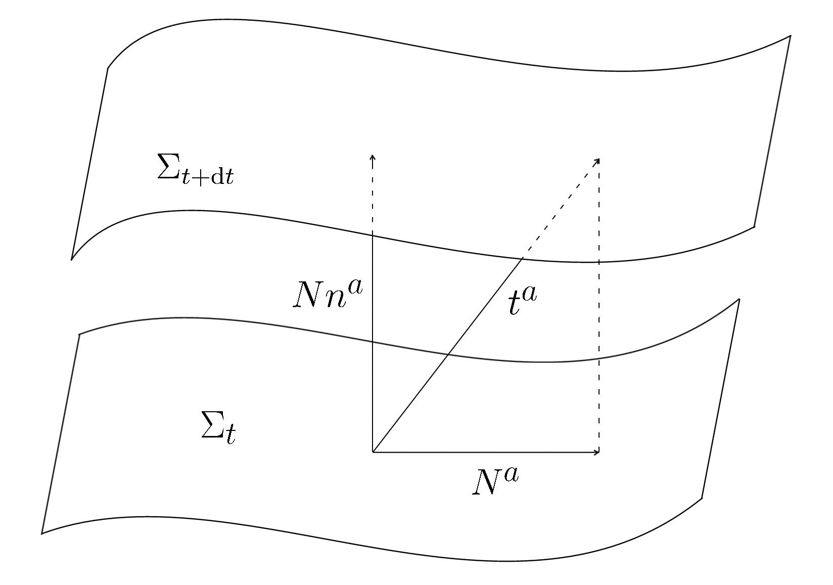
Let be a timelike vector field in defined by
| (23) |
This vector field identifies points on infinitesimally close hypersurfaces of constant , providing a flow of time that is used for the evolution. We can decompose into its normal and tangential parts as
| (24) |
where is the lapse function and , which is tangential, is the shift vector. Relevantly, the fact that must be timelike implies that . Broadly speaking, gives the rate of change of physical time as compared with . On the other hand, tells us how the coordinates are transported from to . Fig. 1 illustrates this construction.
We define the derivative operator on , , by
| (25) |
where is a tangential tensor. Importantly, one can readily show that this is the only (torsionless) derivative operator such that Wald (1984). Moreover, the time derivative of any tangential tensor is defined by
| (26) |
which is, by construction, a tangential tensor.
One of the dynamical variables we use to describe the evolution of spacetime’s geometry is ; thus, we need to calculate its time derivative. We define
| (27) |
which can be shown to be symmetric. The tensor is known as the extrinsic curvature and it describes the embedding of in . If we use the time derivative on , we obtain
| (28) |
showing that is related to the time derivative of . Given that the equations of motion for UG are second order, it is natural to propose that the appropriate initial data for UG should be given by and .
To end this subsection, we state some expressions that relate the Riemann tensor associated with , , with objects in . One can show that the purely tangential projection of the Riemann tensor satisfies a Gauss-Codazzi relation Wald (1984):
| (29) |
where is the Riemann tensor associated with . In addition, and respectively represent the -dimensional Ricci tensor and curvature scalar. Other projections of the Riemann tensor are
| (30) | |||||
| (31) | |||||
where is a tangential vector field. Some useful relations concerning the projections and the trace of the Ricci tensor are given by
| (32) | |||||
| (34) | |||||
| (35) | |||||
where . Also, we can show that
| (36) | |||||
With this result, Eq. (31) can be written as
| (37) | |||||
These are all the technical results we require. In the next section, we classify the UG equations of motion as evolution or constraints, and study the Cauchy problem for UG.
III Initial value problem
The first task when studying the initial value problem of a theory is to identify the constraints. In this section, we classify the UG field equations into evolution equations and constraints. When working with a geometrical gravity theory with second-order equations of motion, an evolution equation, by definition, contains time derivatives of the extrinsic curvature, which can be thought of as second-time derivatives of . Conversely, an equation with no time derivatives of is a constraint, which must be imposed on the initial data, and, for consistency, must be kept valid under evolution. Notice that we cannot perform the initial value study for generic matter fields without specifying the matter action. Thus, in what follows, vacuum UG is considered; we present the sufficient conditions for the matter action to respect the well-posedness of UG in Subsec. III.3.
In most parts of this section, we consider . Thus, we define as the tensor that, when it vanishes, gives the metric equations of motion, Eq. (9), in the case where . Importantly, in this part of our study, is not assumed to be zero throughout . Instead, a weaker assumption is considered: the constraints are only valid on the initial data hypersurface, while the evolution equations are satisfied all over . Interestingly, we find that dynamical consistency implies in .
From the Bianchi identity, we can show that
| (38) |
Recall that, since we do not assume that vanishes throughout , we cannot claim that its divergence also vanishes, and thus, we cannot argue, at this stage, that is constant. Also, from Eq. (10), we can show that
| (39) |
This last equation allows us to identify the -dimensional trace of tangential-tangential projection with the normal-normal projection, rendering the latter redundant; in what follows, we omit the normal-normal projection. Thus, there are only nine independent components of . These components, together with the unimodular constraint, amount to ten equations, which coincides with the number of independent equations of GR.
We separate into its tangential-tangential projection and its normal-tangential projection, which are respectively given by
| (40) | |||||
| (41) |
where we use Eqs. (32) and (34). The tangential-tangential projection of the field equation, Eq. (40), has time derivatives of . Therefore, it is an evolution equation. On the other hand, the normal-tangential projection, Eq. (41), does not contain time derivatives of , and it is thus a constraint, which is reminiscent of the GR momentum constraint.
Notice that the unimodular constraint, Eq. (6), is a constraint in the sense that it does not have time derivatives of . Still, it is not a relation that can be imposed on the initial data and that is automatically satisfied throughout spacetime by the evolution. This is because the values of , which is nondynamical, are given a priori all over . However, we will show that the unimodular constraint can be satisfied by choosing the lapse function.
In summary, in terms of components, six of the field equations of vacuum UG, the tangent-tangent projections, are evolution equations, while the remaining three, the normal-tangential projections, are constraints. In the next subsection, we analyze the evolution of the constraints.
III.1 Constraint equations
We now study if the constraint, Eq. (41), is maintained under evolution. In other words, given initial data on that satisfies Eq. (41), we must check if the fields obtained by evolving this initial data still satisfy the constraint. This can be done by proving that the constraints on the initial data hypersurface have zero time derivative. Without loss of generality, we take the initial value hypersurface to be .
We define the tangential tensors
| (42) | |||||
| (43) |
Let be the following set of assumptions: the evolution equations, , are valid throughout , and the constraint, , is only valid on . What remains to check is if, under , on . From the definition of the time derivative, we readily obtain
| (44) | |||||
Given that on , Eq. (44), when restricted to , takes the form
| (45) |
which is not automatically zero under .
Let
| (46) |
Clearly, the time derivative of vanishes if . We can show that, under , on :
Proof.
According to Dirac’s method Dirac (2001), it is necessary to promote as a constraint; in Dirac’s terminology, is a “secondary constraint.” This, of course, implies that the -dimensional curvature scalar, , must be constant throughout . Namely, , where . Notice that we must consider as a shorthand notation for the right-hand side of Eq. (35), which only contains tangential objects. Also, as the notation suggests, will end up playing the role of the cosmological constant. However, at this stage, we can only claim that is constant along and there is no reason to assume that ; dynamical consistency fixes to be constant throughout spacetime, as we show next.
We now prove that, under , on :
Proof.
Using the fact that is the identity tensor in spacetime, we can verify that
| (52) |
The divergence of this last equation produces
| (53) |
Alternatively, we can calculate using the Leibniz rule and Eq. (38), producing
| (54) |
When we compare Eqs. (53) and (54), we obtain
| (55) |
where we use . Hence, on and assuming ,
| (56) |
This result, together with the fact that on , implies that on . ∎
The lesson from the last proof is that, under , is constant throughout . Recall that is a significantly weaker set of assumptions than assuming that throughout . We now need to check if on , assuming and ; we refer to this set of assumptions by . Clearly, under , the vanishing of is equivalent to
| (57) |
which we show to hold:
Proof.
Using Eq. (50), we get
| (58) | |||||
where we write and in terms of and other tangential objects using Eqs. (35) and (36). Notice that, except for the first term, all the terms in Eq. (58) are proportional to , , , or derivatives of and , all of which vanish under . Thus, we need to focus on
where we repeatedly use the definition of the tangential derivative, the Leibniz rule, and the fact that covariant derivatives acting on scalars commute; this is a consequence of the torsion-free hypothesis (a study of an unimodular theory with torsion is presented in Ref. Bonder and Corral, 2018). When we evaluate on , the first and last terms in Eq. (LABEL:42) can be seen to vanish using . Moreover, if we take the tangential derivative of Eq. (55), we can write the second term in terms of objects that also vanish under . With all this, we can show that, under , on . ∎
Relevantly, the secondary constraint can be written in a more familiar way. Starting from , which, under , is equivalent to , and using and Eqs. (35) and (49), it is possible to obtain
| (60) |
which has the form of the Hamiltonian constraint of GR with a cosmological constant. However, in vacuum UG, Eq. (60) appeared for dynamical consistency and not as a (primary) constraint. The main conclusion of this subsection is that, for consistency, initial data in vacuum UG must be subject to Eqs. (41) and (60). In the next subsection, we verify that the evolution predicted in vacuum UG is unique, continuous, and causal in the above-described sense.
III.2 Evolution equations
In this subsection, we study the evolution equations, namely, the tangential-tangential projection of the vacuum field equations, and the unimodular constraint. We have taken and as the dynamic variables for vacuum UG. However, an approach that better adapts to our needs is the BSSN formulation, developed for GR initially by Shibata and Nakamura Shibata and Nakamura (1995) and later by Baumgarte and Shapiro Baumgarte and Shapiro (1998). The BSSN formulation consists of separating the conformal factor for the spatial metric and the trace of the extrinsic curvature, and studying their evolution separately. Also, we decompose the tensors into their components on the foliation hypersurfaces, which are denoted with Latin indexes . Also, for simplicity, we take , a condition that can be trivially relaxed.
Let be such that
| (61) |
where
| (62) |
so that the determinant of is ( the determinant associated with ). Notice that
| (63) |
is the inverse of . Moreover, let be the symmetric tensor field defined by
| (64) |
Clearly , namely, is the traceless part of the extrinsic curvature.
In the BSSN formulation the dynamical varialbes are , , , and , which are given by
| (65a) | |||||
| (65b) | |||||
| (65c) | |||||
| (65d) | |||||
| (65e) | |||||
The first expression is a redefinition of the conformal factor, the second is the trace of the extrinsic curvature, the third is the conformal transformation given in Eq. (61), the fourth is a rescaling of the traceless part of the extrinsic curvature, and finally, are the conformal connection functions, where
| (66) |
are the Christoffel symbols associated with . Furthermore, we can show that Eq. (65e) is equivalent to
| (67) |
What remains to be done is to rewrite the constraint and evolution equations in terms of the BSSN variables; this allows us to argue when comparing with the GR evolution equations, that vacuum UG has a well-posed initial value formulation.
Using Eq. (60) we can cast the evolution equation, Eq. (40), as
| (68) | |||||
which coincides with the evolution equation of GR with a cosmological constant. Thus, the system of evolution equations of vacuum UG, in BSSN variables, takes the same form of the corresponding GR equations, namely,
| (69a) | |||||
| (69b) | |||||
| (69c) | |||||
| (69d) | |||||
| (69e) | |||||
Given that GR with a cosmological constant is strongly hyperbolic Sarbach et al. (2002), then, it follows from our analysis that the evolution equations of vacuum UG are also strongly hyperbolic, and thus, this theory has a well-posed evolution in the sense of being unique, continuous, and causal.
We turn now to discuss the unimodular constraint. Using the well-known expression and Eq. (65a), we get . On the other hand, the unimodular constraint is . By direct comparison, we can conclude that the unimodular constraint is satisfied as long as
| (70) |
Notably, both sides of Eq. (70) must be positive. Moreover, the fact that the unimodular constraint can be solved by simply choosing the lapse function is compatible with the result of Ref. Bengochea et al. (2023) where it is noted that one component of the metric is sufficient to solve the unimodular constraint.
With this analysis, we shown that vacuum UG has an evolution that is unique, continuous, and causal. However, there are cases where the initial data must be given on different charts covering . In this case, a “gluing” of the different “evolutions” must be made. Fortunately, this procedure can be carried out in the same manner as in GR Wald (1984), since this procedure relies on making coordinate transformations, which are available in UG. Likewise, there is no obstruction to applying the GR proof Choquet-Bruhat and Geroch (1969) that shows that there is a maximal evolution of the initial data. Therefore, we can conclude that vacuum UG has a well-posed initial value formulation which gives rise to a maximal evolution of the initial data. In the next subsection, we discuss UG with matter.
III.3 Initial value formulation with matter
The initial value formulation of a UG theory with matter can only be studied once the relevant matter action is given. Still, we provide a set of sufficient conditions to have a well-posed initial value formulation for a UG theory with a generic matter action. Of course, the methods we present can be used for a particular matter action.
The metric field equation is equivalent to , as in Eq. (9). Again, we do not assume that vanishes in , but only a weaker assumption: the constraints vanish on and the evolution equations vanish in . Importantly, we can check that
| (71) |
where we use Eq. (19).
The tangential-tangential projection and normal-tangential projection of are respectively given by
| (72) | |||||
| (73) |
which are tangential tensors. Recall that, since , the normal-normal projection of can be obtained from Eq. (72).
We know, from the vacuum UG analysis, that Eq. (72) is an evolution equation. On the other hand, the normal-tangential projection, Eq. (73), is a constraint provided that can be written in such a way that it does not contain second time derivatives of or the matter fields. Assuming this is the case, we find the conditions necessary for the constraint to remain valid under evolution. This analysis can be done as in Subsec. III.1, the main difference is that now is constant, as expected from Eq. (71). The conclusion is that, to have dynamical consistency, the initial data must be subject to
| (74) | |||||
| (75) |
where, to write Eq. (75) in this form, we take the trace of Eq. (72) and we use that . Equation (75) looks like the Hamiltonian constraint with matter and a cosmologican constant but it depends on , which, recall, is closely related to ; this is an important difference when comparing with GR.
We can study the well-posedness of the evolution equations with matter in a simple way. Mimicking the analysis of vacuum UG in terms of BSSN variables, we can show that the UG evolution equations have the same form as those of GR with matter and a cosmological constant, but in this case plays the role of the cosmological constant. Now, it is known that GR with matter and a cosmological constant has a well-posed initial value formulation, in a weak hyperbolic sense Nagy et al. (2004); Reula (1998), provided that only depends on the fields and its first derivatives and that the matter equations of motion, Eq. (7), are also well-posed by themselves. To prove this result one can use the fact that the evolution equations are quasilinear, diagonal, second-order hyperbolic (QDSOH), and apply Leray’s theorem Leray (1953), as done in Ref. Wald, 1984. We can thus conclude that UG has a well-posed initial value formulation as long as neither nor , which also appears in the dynamical equations, have second derivatives of the fields, and the matter field equations are well posed. Observe that this restriction on the energy-momentum tensor is enough for Eq. (73) to be a constraint. Of course, these are sufficient conditions; there could be cases that do not meet this hypothesis and still have a well-posed initial value formulation.
IV Conclusions
One of the most important properties of any theory is its capacity to make predictions out of initial data. Therefore, if UG is to be considered as a viable physical theory, it needs to have a well-posed initial value formulation. Moreover, to utilize this theory, we need to find all the constraints. Here, we show that UG is well-posed and we find all the constraints. For the latter, we followed the well-known Dirac method; the result is that there are primary constraints, , and secondary constraints, . Then, we used these constraints in the evolution equations to cast them in the form of those in GR, which have a well-posed initial value formulation, completing the proposed analysis.
Remarkably, the unimodular constraint does not behave as a constraint in the sense that it is not imposed on the initial data and preserved under evolution. This feature ought to be present in any theory with nondynamical fields, like the gravitational sector of the Standard Model Extension Kostelecký (2004). In the present case, the unimodular constraint can always be satisfied by a choice of the lapse function, shedding some light on the role of the UG nondynamical function.
We also found interesting that the equivalence between GR and vacuum UG, in the context of an initial value problem, is not a priori obvious even when is constant. Interestingly, only by requiring dynamical consistency does a spacetime constant emerge (e.g., in vacuum) that can be used to show this equivalence. Still, UG can be a suitable test theory to perform numerical computation of modified geometrical gravity theories. In addition, the results we obtain suggest that one can run GR numerical calculations using only the traceless part of the Einstein equations. Of course, the relevant case when looking for new physical phenomena is to allow for .
Finally, UG has more constraints than the constraints of GR. This enhanced number should be related to the reduced symmetries of UG Henneaux and Teitelboim (1992), but a detailed counting of constraints is not direct Henneaux and Teitelboim (1989). For that, we would need to use Hamiltonian methods, which have been used to study the problem of time in UG Unruh (1989); Smolin (2009). Unfortunately, other studies of theories with nondynamical fields Reyes and Schreck (2021); Bonder (2023) suggest that a full Hamiltonian analysis should not be straightforward.
Acknowledgements.
We acknowledge getting valuable feedback from M. Chernicoff, U. Nucamendi, N. Ortiz, M. Salgado, O. Sarbach, and D. Sudarsky. This project used financial support from CONAHCyT FORDECYT-PRONACES grant 140630 and UNAM DGAPA-PAPIIT grant IN101724.References
- Weinberg (1989) S. Weinberg, Rev. Mod. Phys. 61, 1 (1989).
- Wald (1984) R. M. Wald, General Relativity (Chicago Univ. Press, 1984).
- Choquet-Bruhat and Geroch (1969) Y. Choquet-Bruhat and R. Geroch, Comm. Math. Phys. 14, 329 (1969).
- Salgado (2006) M. Salgado, Class. Quantum Grav. 23, 4719 (2006).
- Rendall (2006) A. D. Rendall, Class. Quantum Grav. 23, 1557 (2006).
- Sarbach et al. (2019) O. Sarbach, E. Barausse, and J. A. Preciado-López, Class. Quantum Grav. 36, 165007 (2019).
- Kovács (2019) A. D. Kovács, Phys. Rev. D 100, 024005 (2019).
- Kovács and Reall (2020) A. D. Kovács and H. S. Reall, Phys. Rev. D 101, 124003 (2020).
- Saló et al. (2022) L. A. Saló, K. Clough, and P. Figueras, Phys. Rev. Lett. 129, 261104 (2022).
- Einstein (1919) A. Einstein, Sitzungsber. Preuss. Akad. Wiss. Berlin , 349 (1919), with an English translation in The Principle of Relativity (Dover Publications, 1952).
- Pauli (1981) W. Pauli, Theory of relativity (Courier Dover Publications, 1981).
- Álvarez and Velasco-Aja (2023) E. Álvarez and E. Velasco-Aja, “A primer on unimodular gravity,” (2023), arXiv:2301.07641 [gr-qc] .
- Anderson and Finkelstein (1971) J. L. Anderson and D. Finkelstein, Am. J. Phys. 39, 901 (1971).
- van der Bij et al. (1982) J. J. van der Bij, H. van Dam, and Y. J. Ng, Physica 116A, 307 (1982).
- Buchmuller and Dragon (1988) W. Buchmuller and N. Dragon, Phys. Lett. B 207, 292 (1988).
- Buchmuller and Dragon (1989) W. Buchmuller and N. Dragon, Phys. Lett. B 223, 313 (1989).
- Ellis et al. (2011) G. F. R. Ellis, H. van Elst, J. Murugan, and J.-P. Uzan, Class. Quantum Grav. 28, 225007 (2011).
- Earman (2022) J. Earman, “Trace-free gravitational theory (aka unimodular gravity) for philosophers,” (2022), https://philsci-archive.pitt.edu/20765.
- Josset et al. (2017) T. Josset, A. Perez, and D. Sudarsky, Phys. Rev. Lett. 118, 021102 (2017).
- Perez and Sudarsky (2019) A. Perez and D. Sudarsky, Phys. Rev. Lett. 122, 221302 (2019).
- Linares Cedeño and Nucamendi (2021) F. X. Linares Cedeño and U. Nucamendi, Phys. Dark Universe 32, 100807 (2021).
- Linares Cedeño and Nucamendi (2023) F. X. Linares Cedeño and U. Nucamendi, JCAP 2023, 036 (2023).
- Carballo-Rubio et al. (2022) R. Carballo-Rubio, L. J. Garay, and G. García-Moreno, Class. Quantum Grav. 39, 243001 (2022).
- Bonder et al. (2023) Y. Bonder, J. E. Herrera, and A. M. Rubiol, Phys. Rev. D 107, 084032 (2023).
- Corral and Bonder (2019) C. Corral and Y. Bonder, Class. Quantum Grav. 36, 045002 (2019).
- Nakahara (2016) M. Nakahara, Geometry, Topology and Physics, 3rd ed. (Taylor & Francis, 2016).
- Dirac (2001) P. Dirac, Lectures on Quantum Mechanics (Dover Publications, 2001).
- Bonder and Corral (2018) Y. Bonder and C. Corral, Phys. Rev. D 97, 084001 (2018).
- Shibata and Nakamura (1995) M. Shibata and T. Nakamura, Phys. Rev. D 52, 5428 (1995).
- Baumgarte and Shapiro (1998) T. W. Baumgarte and S. L. Shapiro, Phys. Rev. D 59, 024007 (1998).
- Sarbach et al. (2002) O. Sarbach, G. Calabrese, J. Pullin, and M. Tiglio, Phys. Rev. D 66, 064002 (2002).
- Bengochea et al. (2023) G. R. Bengochea, G. León, A. Perez, and D. Sudarsky, JCAP 2023, 011 (2023).
- Nagy et al. (2004) G. Nagy, O. E. Ortiz, and O. A. Reula, Phys. Rev. D 70, 044012 (2004).
- Reula (1998) O. A. Reula, Liv. Rev. Rel. 1, 1998 (1998).
- Leray (1953) J. Leray, “Hyperbolic differential equations,” (1953), https://hdl.handle.net/20.500.12111/8019.
- Kostelecký (2004) V. A. Kostelecký, Phys. Rev. D 69, 105009 (2004).
- Henneaux and Teitelboim (1992) M. Henneaux and C. Teitelboim, Quantization of Gauge Systems (Princeton University Press, 1992).
- Henneaux and Teitelboim (1989) M. Henneaux and C. Teitelboim, Phys. Lett. B 222, 195 (1989).
- Unruh (1989) W. G. Unruh, Phys. Rev. D 40, 1048 (1989).
- Smolin (2009) L. Smolin, Phys. Rev. D 80, 084003 (2009).
- Reyes and Schreck (2021) C. M. Reyes and M. Schreck, Phys. Rev. D 104, 124042 (2021).
- Bonder (2023) Y. Bonder, in Proceedings of the Ninth Meeting on CPT and Lorentz Symmetry (World Scientific, 2023) p. 176.