Critical behavior of the Fredenhagen-Marcu order parameter at topological phase transitions

Abstract

A nonlocal string order parameter detecting topological phase transitions has been proposed by Fredenhagen and Marcu (FM). In this work, we find that the FM string order parameter for the toric code in a magnetic field exhibits universal scaling behavior near critical points by directly evaluating it in the infinite string-length limit using infinite Projected Entangled Pair States (iPEPS). Our results thus indicate that the FM string order parameter is a quantitatively good order parameter to characterize topological phase transitions. In the presence of the electric-magnetic duality symmetry, a novel critical exponent can be extracted from the FM string order parameter, which is consistent with the (2+1)D XY universality class. In addition, we argue that only in the regime with emergent 1-form Wilson loop symmetry, the corresponding FM string order parameter can faithfully detect the topological transition.

Introduction. Since the discovery of the fractional quantum Hall effect [1, 2], topological phases of matter have been intensively explored. Exactly solvable models have been constructed [3, 4, 5], and a mathematical framework for classifying topological phases of matter has been developed [6, 7]. Recently, various topologically ordered states have been experimentally investigated with quantum computers and simulators as well [8, 9, 10]. Unlike conventional phases of matter, topological phases cannot be characterized by simple local order parameters. Instead non-local string order parameters are required, as proposed by Fredenhagen and Marcu (FM) in the context of the $\mathbb{Z}_{2}$ gauge-Higgs model [11, 12]. Recently, this FM string order parameter has also been used to detect $\mathbb{Z}_{2}$ topological order in a quantum dimer model realized by the Rydberg quantum simulator [13, 9]. However, due to its non-local nature the FM string order parameter remains challenging to be understood, in particular, in the long-string limit and in the vicinity of critical points.

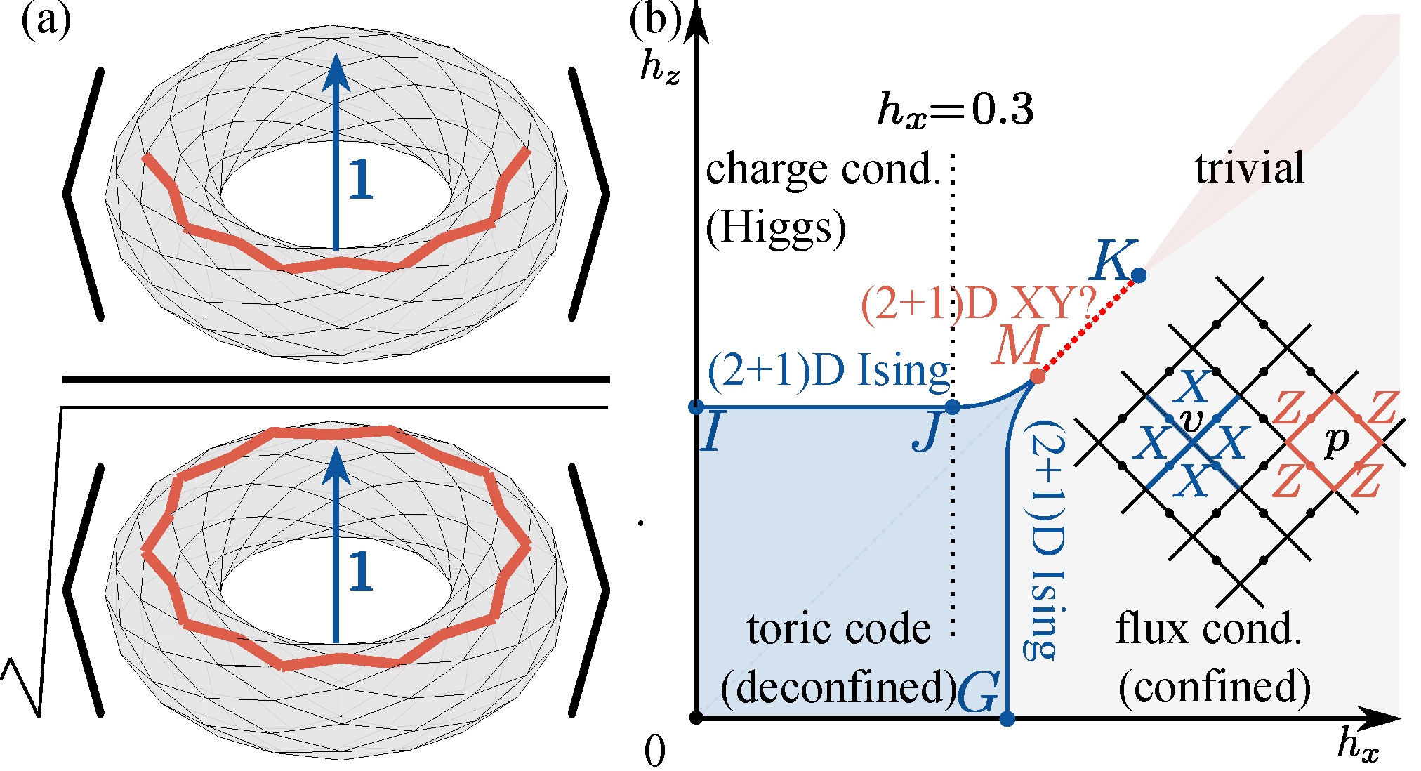
Figure 1: FM string order parameter and phase diagram. (a) Schematic of the FM string order parameter, where black lines indicate the underlying lattice on a torus, red lines are a string and a loop of $Z$ operators, and $\boldsymbol{1}$ is the trivial anyon flux penetrating through the torus. (b) Phase diagram of the toric code model in a field. Charges are deconfined in the toric code phase. For strong fields, nearby the $h_{z}$ ($h_{x}$) axis, charges condense (are confined), corresponding to the Higgs (confined) region in the context of gauge theories. We argue that the FM string order parameter (dual FM string order parameter) associated with charges (fluxes) can only detect the transition in the regime with an emergent 1-form Wilson (’t Hooft) loop symmetry in the blue and white (gray) area. In the the light red area, both the Wilson and ’t Hooft loop symmetries can not emerge. Inset: definition of the vertex and the plaquette operators on a square lattice.

In this work, we show how to evaluate the FM string order parameter shown in Fig. 1a, in the limit of an infinitely long string using transfer matrices of infinite Projected Entangled Pair States (iPEPS). We apply this method to study the FM string order parameter of the toric code model in a field. Technically, we approximate ground states of the model using iPEPS based on the energy gradient optimization [14, 15], which is calculated by the automatic differentiation [16]. We find that near the topological transition between the toric code and the Higgs region, Fig. 1b, the FM string order parameter exhibits a critical exponent of the $(2+1)$D Ising universality class. In the presence of the electric-magnetic (EM) duality symmetry, the FM string order parameter exhibits a new critical exponent, which is different from that of the local order parameter studied before [17, 18, 19]. The universality of this multi-critical point has been recently under debate [17, 18, 19, 20]. We find that the critical exponent is compatible with the $(2+1)$D XY universality class. Our results show that the FM string order parameter exhibits universal scaling behavior near critical points, suggesting that the FM string order parameter is a quantitatively good order parameter for topological phase transitions. However, we also argue that the FM string order parameter containing a string operator with electric charges at the ends can only detect the topological transition in the regime with an emergent 1-from Wilson loop symmetry [blue and white shaded regions in Fig. 1b]. A dual FM string order parameter associated with magnetic flux is required to detect the topological phase transition in the regime with an emergent 1-form ’t Hooft loop symmetry [blue and gray shaded region in Fig. 1b].

Toric code model and the FM string order parameter. We consider the toric code model on a square lattice in a field:

$$H_{\text{TC}}(h_{x},h_{z})=-\sum_{v}A_{v}-\sum_{p}B_{p}-h_{x}\sum_{e}X_{e}-h_{z}\sum_{e}Z_{e},$$ (1)

where $A_{v}=\prod_{e\in v}X_{e}$ and $B_{p}=\prod_{e\in p}Z_{e}$ are the vertex and plaquette operators, as shown in the inset of Fig. 1b, and $X_{e}$ and $Z_{e}$ are Pauli matrices defined on the edges $e$ of the lattice. The phase diagram of the model in Fig. 1b is well-known [21, 22, 23]. There is a toric code phase at weak fields and a trivial phase at strong fields.

At $h_{x}=0$, the toric code model in Eq. (1) has an exact 1-form Wilson loop symmetry: $\left[\prod_{e\in L}Z_{e},H_{\text{TC}}(0,h_{z})\right]=0,\forall L$, where $L$ is a closed loop along the primal lattice. Thus a string operator $\prod_{e\in L_{1/2}}Z_{e}$ can create a pair of charges at its two ends, where $L_{1/2}$ is an open string along the primal lattice, and a string order parameter $\tilde{O}_{Z}$ can be constructed to detect charge condensation [24]:

$$\tilde{O}_{Z}=\lim_{|L_{1/2}|\rightarrow\infty}\sqrt{|\tilde{C}_{Z}(|L_{1/2}|)|},\quad\quad\tilde{C}_{Z}(|L_{1/2}|)=\langle{\Psi}|\prod_{e\in L_{1/2}}Z_{e}|{\Psi}\rangle,$$ (2)

where $\ket{\Psi}$ is a normalized ground state of the toric code model, $|L_{1/2}|$ is the distance between two ends of $L_{1/2}$. The bulk of the string order parameter $\tilde{O}_{Z}$ commutes with the overlapping local Hamiltonian terms but not its ends. In the toric code phase, the string order parameter thus creates two anyonic charge excitations which are orthogonal to the ground state, leading to a vanishing string order parameter in the infinite string limit, $\tilde{O}_{Z}=0$. By contrast, in the Higgs phase, the string order parameter can be nonzero because the $h_{z}$ field induces charge fluctuations such that charges condense in the Higgs phase. An alternative way of interpreting this string operator is by mapping $H_{\text{TC}}(0,h_{z})$ to the $(2+1)$D transverse field Ising model [25, 26]. This transforms $\tilde{O}_{Z}$ and $\tilde{C}_{Z}$ to the Ising order parameter and its correlation function, respectively. From that also follows directly that the the critical point $I$ [see Fig. 1b] at $h_{z}=h_{zc}^{(I)}=0.328474(3)$ [27] belongs to the (2+1)D Ising universality class . Near the critical point $I$: $\tilde{O}_{Z}\sim(h_{z}-h_{zc}^{(I)})^{\beta}$ and $\xi\sim(h_{z}-h_{zc}^{(I)})^{-\nu}$, where $\beta=0.326418(2)$ is the critical exponent of the order parameter [29], $\xi$ is the correlation length defined via $|\tilde{C}_{Z}(|L_{1/2}|)-\tilde{O}_{Z}^{2}|\sim e^{-|L_{1/2}|/\xi}$, and $\nu=0.629970(4)$ is the critical exponent of the correlation length [29].

When $h_{x}\neq 0$, the Wilson loop operator $\prod_{e\in L}Z_{e}$ is no longer an exact 1-form symmetry of the toric code model and the bulk of the string $\prod_{e\in L_{1/2}}Z_{e}$ cannot deform freely. Therefore $\tilde{C}_{Z}(|L_{1/2}|)$ vanishes on either side of the topological phase transition exponentially with the length of the string $|L_{1/2}|$. However, when $h_{x}$ is small, the toric code model has an emergent 1-form Wilson loop symmetry [30, 31, 32]. In the limit of large $h_{x}$, the 1-form Wilson loop symmetry cannot emerge, which we indicate by the gray area in Fig. 1b. The boundary with and without emergent Wilson loop symmetry has been argued to be given by a percolation transition [33, 17]. In the presence of an emergent 1-form Wilson loop symmetry, one can in principle conceive to construct a dressed string operator with an extended width [34, 31]. This is however a challenging task in practice. This problem can be circumvented, by dividing out the “bulk” contribution of the string order paramter, as proposed by Fredenhagen and Marcu, leading to the FM string order parameter [11, 12]:

$$O_{Z}=\lim_{r\rightarrow\infty}\sqrt{|C_{Z}(r)|},\,\,\quad C_{Z}(r)=\frac{\langle{\Psi}|\prod_{e\in L_{1/2}}Z_{e}|{\Psi}\rangle}{\sqrt{\bra{\Psi}\prod_{e\in L}Z_{e}\ket{\Psi}}},$$ (3)

where $r=|L_{1/2}|$ is the length of the string $L_{1/2}$ , $L$ is a loop whose length is twice the length of the string $L_{1/2}$, see Fig. 1a. Compared to Eq. (2), the FM string order parameter in Eq. (3) contains a square root of the expectation value of the Wilson loop operator in the denominator. When $h_{x}\neq 0$ the bare Wilson loop operator is no longer a symmetry and its expectation values decays as the perimeter law: $\bra{\Psi}\prod_{e\in L}Z_{e}\ket{\Psi}\sim\exp(-\alpha_{Z}|L|)$, where $\alpha_{Z}$ is the parameter law coefficient and $|L|$ is the length of the loop $L$. The denominator in the FM string order parameter compensates the perimeter law decay such that only the contribution from the endpoints of the string $L_{1/2}$ is taken into account.

On a torus, the loop $L$ can be either contractible or non-contractible. When $L$ is a non-contractible loop, which is convenient for tensor network methods, the denominator in Eq. (3) depends on the choice of the topologically degenerate ground states in the toric code phase. We show that the contractible and non-contractible loops are equivalent when the ground state is chosen as the minimally entangled state with a trivial anyon flux penetrating through the torus [36], as shown in Fig. 1a; for details see supplement [37].

Figure 2: Evaluating the FM string order parameter using iPEPS. (a) The iPEPS ansatz approximating a ground state of the toric code model with a bond dimension $D$, where the gray lines are the primal lattice. (b) The $A$ and $B$ tensors are related by a $\pi/2$ rotation. A double tensor contracting the physical leg and another double tensor sandwiching a $Z$ operator can be constructed from the iPEPS tensor. (c) Using the double tensors, two iPEPS transfer matrices are defined, which we use to evaluate the FM string order parameter in Eq. (Critical behavior of the Fredenhagen-Marcu order parameter at topological phase transitions).

iPEPS method. We now discuss how to evaluate the FM string order parameter efficiently in the limit of an infinitely long string using transfer matrices of iPEPS. To this end, we construct from the iPEPS of the ground state two transfer matrices, one is the usual transfer matrix $\mathbb{T}$ and the other is $\mathbb{T}_{Z}$ containing some $Z$ operators; see Fig. 2 for graphical notations. With that the FM order parameter can be calculated as follows. The numerator consists of $r$ transfer matrices $\mathbb{T}$ followed by $r$ transfer matrices $\mathbb{T}_{Z}$ containing a $Z$ string and the denominator consists of $2r$ transfer matrices $\mathbb{T}_{Z}$ containing a $Z$ loop:

$$O_{Z} =\lim_{r\rightarrow\infty}\left[\frac{\Tr(\mathbb{T}^{r}\mathbb{T}_{Z}^{r})/\Tr(\mathbb{T}^{2r})}{\sqrt{\Tr(\mathbb{T}_{Z}^{2r})/\Tr(\mathbb{T}^{2r})}}\right]^{1/2}=\lim_{r\rightarrow\infty}\frac{t^{\frac{r}{2}}t_{Z}^{\frac{r}{2}}/t^{r}}{t_{Z}^{\frac{r}{2}}/t^{\frac{r}{2}}}|\innerproduct{V}{V_{Z}}|$$

$$=|\innerproduct{V}{V_{Z}}|,$$ (4)

where in the limit of $r\to\infty$, the action of the transfer matrices is set by the dominating eigenvalue and eigenvector, $\mathbb{T}_{Z}^{\infty}=t_{Z}^{\infty}\ket{V_{Z}}\bra{V_{Z}}$ and $\mathbb{T}^{\infty}=t^{\infty}\ket{V}\bra{V}$. Here, $V$ and $V_{Z}$ are fixed points of $\mathbb{T}$ and $\mathbb{T}_{Z}$, respectively. We use $\Tr(\mathbb{T}^{2r})$ to explicitly normalize the iPEPS. The perimeter law coefficient can be obtained from the dominant eigenvalues of the transfer matrices: $\alpha_{Z}=-\log(t_{Z}/t)$. A more detailed and rigorous derivation can be found in supplement [37].

In order to evaluate the FM string order parameter it remains to solve for the iPEPS ground states of the toric code model in Eq. (1). We use the iPEPS ansatz proposed in Ref. [38] to approximate a ground state of the Hamiltonian (1); Fig. 2a. We optimize the iPEPS using a gradient-based optimization [14, 15], and compute the gradient of the energy density using automatic differentiation [16], see technical details in the supplement [37]. There are two important parameters that systematically control the error of the approximation: the bond dimension $D$ of the iPEPS itself (see Fig. 2a) and the bond dimension $\chi$ of the environment of the iPEPS; the larger bond dimensions provide better approximations.

We first validate our method by comparing the ground state energy density and expectation values of local Hamiltonian terms from our optimized iPEPS and quantum Monte Carlo (QMC) simulations [21], see details in supplement [37]. By extrapolating the peak positions of iPEPS correlation length from various bond dimensions, we approximately determine the position of the critical point $J$ in Fig. 1a as $h_{z}=h^{(J)}_{zc}=0.335(1)$, which is close to the result $h^{(J)}_{zc}=0.333(1)$ in Ref. [21]. Using the same method, we find that the multi-critical point $M$ shown in Fig. 1b as $h^{(M)}_{zc}=0.3397(2)$, which is close to $h_{zc}^{(M)}=0.340(2)$ of Ref.[21] and $h_{zc}^{(M)}=0.3406(4)$ of Ref. [22]. We estimate that the position of the critical endpoint $K$ is $h_{zc}^{(K)}=0.421(2)$, which is consistent with $h_{zc}^{(K)}=0.418(2)$ of Ref. [21].

Results of the FM string order parameter along $\boldsymbol{h_{x}=0.3}$. Having introduced the framework for evaluating the FM string order parameter in the limit of infinitely long strings, we now evaluate it numerically along $h_{x}=0.3$ from iPEPS with various bond dimensions; see Fig. 3a. In the toric code phase the FM string order parameter vanishes while it is finite in the Higgs phase. We also extract the critical exponent $\beta_{\text{FM}}$ defined via $O_{Z}\sim(h_{z}-h^{(J)}_{zc})^{\beta_{\text{FM}}}$, Fig. 3c, where we obtain $O_{Z}$ by performing linear extrapolation in $1/D$ and ignore the small $\chi$ dependence. The extracted critical exponents $\beta_{\text{FM}}=0.33(5)$ is consistent with the exponent $\beta=0.326418(2)$ of the $(2+1)$ D Ising universality class [29]. We furthermore collapse the data from different bond dimensions, as shown in Fig. 3b, based on the theory of finite entanglement scaling [39, 40, 41]. The data for $D>2$ indeed collapses on a single curve near criticality. These results indicate that the critical behavior of the FM string order parameter near the critical point $J$ is controlled by the $(2+1)$D Ising universality class.

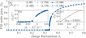
Figure 3: FM string order parameter along $h_{x}=0.3$. (a) FM string order parameter from iPEPS with various bond dimensions $(D,\chi)$, see legend. (b) Data collapse of the FM string order parameter with $\nu=0.629970(4)$ and $\beta=0.326418(2)$. (c) Double-log plot extracting the critical exponent $\beta_{\text{FM}}$ by linearly extrapolating $O_{Z}$ in $1/D$, where we we used $h_{zc}=0.335(1)$.

Previous order parameters for topological phase transitions were defined on the virtual legs of the iPEPS [42, 43, 44, 45, 46], because there exist the virtual symmetries in terms of matrix product operators [47, 48, 49]. However, without the iPEPS representation, these virtual order parameters cannot be obtained, i.e., they are not physical. This is in contrast to the FM string order parameter that is defined on the physical level and thus also does not depend on the iPEPS gauge. Moreover, the FM string order parameter defined in Eq. (3) can be applied to other charge condensation phase transitions with different universality classes, i.e., near the charge condensation phase transition of a toric code ground state deformed by two string tensions [50, 51, 52]. We evaluate the FM string order parameter also for this case and show that it exhibits a critical exponent $\beta_{\text{FM}}=0.117(5)$ close to $\beta=1/8$ of the $(2+0)$D Ising universality class that characterizes this transition [37].

Results of the FM string order parameter along the self-dual line $h_{x}=h_{z}$. Along the self-dual line, the toric code model in Eq. (1) has a global electric-magnetic duality symmetry, which exchanges the primal lattice and the dual lattice, as well as $X$ and $Z$. There is a gapped electric-magnetic duality symmetry breaking phase $MK$ along the self-dual line [21, 17]. Thus the phase transition crossing the multi-critical point $M$ can be characterized by a local symmetry-breaking order parameter $|\langle X-Z\rangle|$ shown in Fig. 4a, from which we extract a critical exponent $\beta_{\text{local}}=0.83(5)$ defined via $|\langle X-Z\rangle|\sim(h_{z}-h_{zc}^{(M)})^{\beta_{\text{local}}}$, see Fig. 4c. Our result is consistent with recent Monte Carlo simulation [17]. We also evaluate the FM string order parameter along the self-dual line crossing the multi-critical point $M$; Fig. 4d. And we extract the critical exponent $\beta_{\text{FM}}=0.34(4)$ defined via $O_{Z}\sim(h_{z}-h^{(M)}_{zc})^{\beta_{\text{FM}}}$, Fig. 4f, which is different from the critical exponent of the local symmetry-breaking order parameter $\beta_{\text{local}}=0.83(5)$.

Figure 4: Local duality symmetry-breaking and FM string order parameters along the self-dual line $h_{x}=h_{z}$. (a) Local order parameter from iPEPS with various bond dimensions $(D,\chi)$, see legend. (b) Data collapse of the local order parameter with $\nu_{+}=0.67175(1)$ and $\beta_{-}=0.83048(2)$. (c) Critical exponent $\beta_{\text{local}}$, where $|\langle X-Z\rangle|$ is obtained by linearly extrapolation in $1/D$ and $h^{(M)}_{zc}=0.3397(2)$. (d) FM string order parameter from iPEPS with various bond dimensions, see legend. (e) Data collapse of the FM string order parameter with $\beta_{\phi}=0.34870(7)$. (f) Critical exponent $\beta_{\text{FM}}$, where $O_{Z}$ is again obtained by linearly extrapolation in $1/D$.

How to understand the distinct critical exponents $\beta_{\text{local}}$ and $\beta_{\text{FM}}$? Since the phase boundary $IM$ belongs to the Ising universality class and the FM string order parameter exhibits an Ising critical exponent, we can assume that the FM string order parameter $O_{Z}$ corresponds to a field $\phi_{z}$ of an effective Ginsburg-Landau-Wilson theory describing the Ising transition. When two Ising transition lines $IM$ and $GM$ in Fig. 1b meet at the multi-critical point $M$, it is natural to expect that the effective field theory describing the multi-critical point $M$ is the $O(2)$ model with a Lagrangian $\mathcal{L}=\left(\partial\boldsymbol{\phi}\right)^{2}/2+m^{2}\boldsymbol{\phi}^{2}/2+g\boldsymbol{\phi}^{4}/(4!)$ [17, 18], up to some irrelevant terms. Here $\boldsymbol{\phi}=(\phi_{x},\phi_{z})$ is a two-component vector field with $\phi_{z}$ the field associated with the FM string order parameter and $\phi_{x}$ is another field corresponding to the dual FM order parameter defined using a loop and a string of $X$ operators along the dual lattice. The scaling dimension of $\boldsymbol{\phi}^{2}$ is $\Delta_{+}=1.51136(22)$, $\phi_{x}$ or $\phi_{z}$ has a scaling dimension $\Delta_{\phi}=0.519088(22)$ and $\phi_{x}^{2}-\phi_{z}^{2}$ has a scaling dimension $\Delta_{-}=1.23629(11)$ [53, 29, 54], and the following correspondence can be made: $X+Z\sim\boldsymbol{\phi}^{2}$ and $X-Z\sim\phi_{x}^{2}-\phi_{z}^{2}$ [17, 18, 19], as well as $O_{Z}\sim\phi_{z}$. According to the scaling law, the critical exponent of the correlation length is $\nu_{+}=1/(3-\Delta_{+})=0.67175(1)$, and the critical exponent of the FM string order parameter [local order parameter] is $\beta_{\phi}=\Delta_{\phi}\nu_{+}=0.34870(7)$ [$\beta_{-}=\Delta_{-}\nu_{+}=0.83048(2)$], which is very close to the numerically extracted critical exponent $\beta_{\text{FM}}=0.34(4)$ [$\beta_{\text{local}}=0.83(5)$] in Fig. 4f [c]. We can also check the assumption by performing data collapse of the FM string order parameter and the local order parameter using the critical exponents from the XY universality class separately; Figs. 4b and e. The data with iPEPS bond dimension $D>3$ collapses on a single curve, indicating that the multi-critical point $M$ is consistent with the XY universality class.

Some comments are in order. First, the two degenerate ground states in the duality symmetry-breaking phase correspond to the predominant condensation of charges (fluxes) satisfying $\langle X-Z\rangle<0$ ($\langle X-Z\rangle>0$). Because our FM string order parameter is defined with a $Z$ string, it detects the charge condensation, and thus we should use the charge condensation dominated state to evaluate the FM string order parameter. Otherwise, the FM string order parameter is discontinuous at the multi-critical point $M$, as we show in the supplement [37]. Second, Ref. [17] argues that the multi-critical point $M$ does not belong to the XY universality class because changes and fluxes cannot condense simultaneously. We find that the FM string order parameter in Fig. 4d at the multi-critical point $M$ is zero, implying charges do in fact not condense at $M$. Considering that the electric-magnetic duality symmetry is broken along $MK$, the simultaneous condensation problem is avoided. Moreover, Ref. [52] shows the multi-critical point is (2+0)D XY-type using a deformed toric code state. Because of these reasons, we argue for the multi-critical point $M$ to be described by the XY universality class.

Discussion and outlook. We evaluate the FM string order parameter in the infinite long string limit using the iPEPS simulation and find that it exhibits universal scaling controlled by the nearby critical points. By applying the FM string order parameter to the topological phase transition along the self-dual line crossing the multi-critical point $M$, we find that the multi-critical point $M$ is consistent with the XY universality class. We also show that the FM string order parameter is not always valid and argue that only in the presence of an emergent 1-form Wilson loop symmetry, it can detect topological transitions for the following reasons. First, in the gray region of Fig. 1b without emergent 1-form Wilson loop symmetry, the FM string order parameter is numerically unstable because the denominator decays too fast with the perimeter [37]. A similar observation is mentioned in Refs. [12, 55]. Second, in the toric code phase, the emergent non-contractible Wilson loop symmetry can break spontaneously [56, 57, 58, 32, 59], and the numerical evaluation of the FM string order parameter becomes unstable in this case [37]. Third, the FM string order parameter evaluated from a deformed toric code state [52, 51, 50] jumps between zero and finite values in the confined phase which does not have the emergent 1-form Wilson loop symmetry on non-contractible loops [37]. As no phase transition is crossed within the confined phase, the discontinuities indicate that the FM string order parameter fails in the regime without emergent 1-form Wilson loop symmetry. However, we can use the dual FM string order parameter to detect phase transition from the toric code to the confined phase. One needs take care of these issues when applying the FM string order parameter to the experimental data.

Some open questions regarding the phase diagram of the toric code model and the FM string order parameter deserve further exploration. First, it will be interesting to study whether it is possible to detect the boundary of the white region in Fig. 1b with the emergent Wilson loop symmetry using tensor network methods. Second, the FM string order parameter can be applied to different lattice gauge theories [60], and it is an interesting direction to define the FM string order parameters for Kitaev’s quantum double models [3] and Levin-Wen string-net models [5] and apply them to study various topological phase transitions driven by anyon condensation [61, 44, 45]. Moreover, since the Higgs phase can be interpreted as a 1-form symmetry protected topological phase [24], one could explore the relations of string order parameters and measurement-based quantum computation in two-dimensional systems [62].

Note added. While finalizing the manuscript we became aware of related work on the stability of the FM order parameter [63].

Acknowledgements. We thank Fengcheng Wu and Youjin Deng for providing their original QMC data used in Ref. [21] and Rui-Zheng Huang for many helpful comments. We acknowledge support from the Deutsche Forschungsgemeinschaft (DFG, German Research Foundation) under Germany’s Excellence Strategy–EXC–2111–390814868, TRR 360 – 492547816 and DFG grants No. KN1254/1-2, KN1254/2-1, the European Research Council (ERC) under the European Union’s Horizon 2020 research and innovation programme (grant agreement No. 851161 and No. 771537), as well as the Munich Quantum Valley, which is supported by the Bavarian state government with funds from the Hightech Agenda Bayern Plus.

Data availability – Data, data analysis, and simulation codes are available upon reasonable request on Zenodo [64].

Appendix A Technical details about the iPEPS optimization

In this section, we show the technical details of optimizing the ground states of the toric code model using iPEPS. We approximate a ground state using the iPEPS ansatz proposed in Ref. [38]. The iPEPS has a $2\times 2$ unit cell, and it is parameterized by a rank-5 tensor $A$ ($B$ is obtained from $A$ by a $\pi/2$ rotation) with the virtual bond dimension $D$ and the physical dimension $d=2$, as shown in Figs. 5a and b.

We impose the square lattice symmetry onto the tensor $A$ such that the iPEPS tensor is invariant under two reflections $R_{v}$ and $R_{h}$, see Fig. 5b. Because of the symmetry, the number of independent variational parameters is less than $2D^{4}$, and next we show how to parameterize the tensor $A$. First, we can construct the $2D^{4}\times dD^{4}$ matrix representations of $R_{h}$ and $R_{v}$ applying on the tensor $A$, and a projector $P_{R}=(\mathbbm{1}+R_{h})(\mathbbm{1}+R_{v})/4$. A subspace spanned by the eigenvectors of $P_{R}$ with an eigenvalue 1 is $\{\ket{v_{i}}|P_{R}\ket{v_{i}}=\ket{v_{i}}\}$. If $\innerproduct{v_{i}}{v_{j}}\neq\delta_{ij}$, we can orthonormalize them using the QR decomposition. Reshaping $\ket{v_{i}}$ to the tensors with the dimensions $D\times D\times D\times D\times 2$, we can parameterize the iPEPS tensor as $A=\sum_{i}\lambda_{i}v_{i}$, where $\lambda=\{\lambda_{i}\}$ are variational parameters. If we also want to impose the virtual $\mathbb{Z}_{2}$ symmetry to the tensor $A$ as shown in Fig. 5a, we just need another projector $P_{Z}=(\mathbbm{1}_{D}^{\otimes 4}\otimes\mathbbm{1}_{d}+Z_{D}^{\otimes 4}\otimes\mathbbm{1}_{2})/2$, where $Z_{D}$ is a $D\times D$ matrix representation of the non-trivial element in $\mathbb{Z}_{2}$, i.e., $Z_{D}^{2}=1$; and we consider the projector $P=P_{Z}P_{R}$, where $[P_{Z},P_{R}]=0$. Using the orthonormal basis of the subspace spanned by the eigenvectors of $P$ with the eigenvalue $1$, we can parameterize the tensor $A$ using $\lambda$.

The iPEPS $\ket{\Psi(\lambda)}$ can be constructed from $A(\lambda)$. The energy expectation value $E=\bra{\Psi(\lambda)}H_{\text{TC}}(h_{z},h_{x})\ket{\Psi(\lambda)}/\innerproduct{\Psi(\lambda)}{\Psi(\lambda)}$ can be evaluated by contracting iPEPS $\ket{\Psi(\lambda)}$. We contract (the squared norm of) the iPEPS using the corner transfer matrix renormalization group (CTMRG) algorithm. As shown in Fig. 5d, we approximate the environment of the double tensors (shown in Fig. 1c) in a $2\times 2$ unit cell using corner (rectangles) and edge tensors (squares) with a bond dimension $\chi$. Since we impose the square lattice symmetry to the tensor $A$, we can contract the iPEPS using the symmetric CTMRG [38]. The bond dimensions of the corner and edge tensors grow to $D^{2}\chi$ after absorbing the double tensors, and we should truncate the bond dimension back to $\chi$. Fig. 5e shows that we obtain the isometries (triangles), which can be used to truncate the bond dimensions, using hermitian eigenvalue decomposition, and we just use eigenvectors corresponding to the $\chi$ largest eigenvalues (in absolute value) to construct the isometry. With the isometries, we can update corner and edge tensors, as shown in Fig. 5f.

In order to optimize the iPEPS, one has to provide the energy gradient $\partial E/\partial\lambda$. The best way to calculate the energy gradient is using automatic differentiation (AD) [16], which calculates the gradient through a backward propagation along the computational graph based on the chain rule in calculus. One problem of applying AD to calculate $\partial E/\partial\lambda$ is that the gradient can be infinite when eigenvalues are degenerate. Although one can add a small perturbation to lift the degeneracy, numerical instability can still happen with a small probability. When we get an infinity gradient, we can detach the isometries from the computation graph and get an approximate gradient; a trade-off between the stability and the accuracy. A possibly better solution is to use the approaches shown in Ref. [66].

Given the energy expectation value and its gradient, we use the BFGS (Broyden–Fletcher–Goldfarb–Shanno) algorithm to minimize the energy expectation value. When the optimization is converged, we have an iPEPS $\ket{\Psi(\lambda)}$ approximating a ground state of the TC model. For this work, the iPEPS optimization was performed by PyTorch on the NVIDIA A100 80 GB GPU cards. We use the checkpoint function of PyTorch to reduce the huge memory cost of AD. Moreover, when getting the isometries, we should use the hermitian eigenvalue decomposition rather than singular eigenvalue decomposition, because the former is about ten times faster than the latter on the GPU.

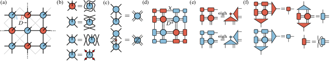
Figure 5: iPEPS ansatz and the CTMRG. (a) The iPEPS ansatz for the ground state of the toric code model with a bond dimension $D$. (b) The iPEPS tensors $A$ and $B$ are related by reflection. The iPEPS tensor $A$ is invariant under two reflections, and we can also impose the virtual $\mathbb{Z}_{2}$ symmetry when necessary, where the red dots are matrices $Z_{D}$. (c) A double tensor and another double tensor sandwiching a $Z$ matrix. (d) The environment of the iPEPS is approximated by the corner tensors (squares) and the edge tensors (rectangles). (e) The hermitian eigenvalue decomposition (eigh) of the top-left corner of the tensor networks in (d), the isometries can be obtained from eigenvectors corresponding to the $\chi$ largest eigenvalues (in absolute value). (f) CTMRG procedures updating the corner and edge tensors using the isometries.

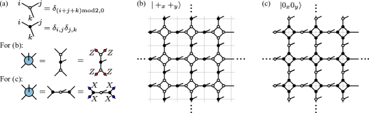
Figure 6: The exact iPEPS at the fixed point $h_{x}=h_{z}=0$ of the toric code phase. (a) The two rank-3 three tensors are define to construct the tensor $A$, and the tensor $A$ for $\ket{+_{x}+_{y}}$ and $\ket{0_{x}0_{y}}$ has different virtual $\mathbb{Z}_{2}$ symmetry. (b), (c) the iPEPS for $\ket{+_{x}+_{y}}$ and $\ket{0_{x}0_{y}}$ on a torus, respectively. The gray lines are the primal lattice.

Appendix B iPEPS for topologically degenerate ground states of the toric code model

In this section, we show two kinds of iPEPS representations of the toric code ground states. Understanding them is useful for initializing the iPEPS optimization and evaluating the FM string order parameter. When $h_{x}=h_{z}=0$, the toric code Hamiltonian defined on a torus commutes with two Wilson loop operators and their dual:

$$W^{Z}_{x}=\prod_{e\in L_{x}}Z_{e},\quad W^{Z}_{y}=\prod_{e\in L_{y}}Z_{e},\quad W^{X}_{x}=\prod_{e\in\hat{L}_{x}}X_{e},\quad W^{X}_{y}=\prod_{e\in\hat{L}_{y}}X_{e},$$ (5)

where $L_{x}$ ($L_{y}$) is a non-contractible loops along $x$($y$) direction on the primal lattice, and $\hat{L}_{x}$ ($\hat{L}_{y}$) is a non-contractible loops along $x$($y$) direction on the dual lattice. They satisfy

$$\left[W_{x}^{Z},W_{y}^{Z}\right]=\left[W_{x}^{X},W_{y}^{X}\right]=\left[W_{x}^{Z},W_{x}^{X}\right]=\left[W_{y}^{Z},W_{y}^{X}\right]=0,\quad\left\{W_{x}^{Z},W_{y}^{X}\right\}=\left\{W_{x}^{X},W_{y}^{Z}\right\}=0.$$ (6)

The four ground states can be labeled eigenvalues of a pair of two commuting loop operators, i.e., common eigenstates of $W^{X}_{x}$ and $W^{X}_{y}$:

$$\ket{+_{x}+_{y}},\quad\ket{+_{x}-_{y}},\quad\ket{-_{x}+_{y}},\quad\ket{-_{x}-_{y}},$$ (7)

or common eigenstates of $W^{Z}_{x}$ and $W^{Z}_{y}$:

$$\ket{0_{x}0_{y}},\quad\ket{0_{x}1_{y}},\quad\ket{1_{x}0_{y}},\quad\ket{1_{x}1_{y}}.$$ (8)

In particular, the common eigenstates of $W_{x}^{Z}$ and $W_{x}^{X}$ (alternatively one can use $W_{y}^{Z}$ and $W_{y}^{X}$) are called minimal entangled state (MES):

$$\ket{0_{x}+_{x}}\equiv\ket{\boldsymbol{1}},\quad\ket{1_{x}+_{x}}\equiv\ket{\boldsymbol{m}},\quad\ket{0_{x}-_{x}}\equiv\ket{\boldsymbol{e}},\quad\ket{1_{x}-_{x}}\equiv\ket{\boldsymbol{f}}.$$ (9)

Let us focus on the ground states $\ket{0_{x}0_{y}}$ and $\ket{+_{x}+_{y}}$, which are exactly the so-called “single-line” and “double-line” iPEPS with the toroidal boundary condition [67]. They are included in the $2\times 2$ unit cell iPEPS ansatz in Fig. 5a. As shown in Fig. 6a, by defining two of rank-3 tensors, we can obtain the $A$ tensor for the iPEPS $\ket{+_{x}+_{y}}$ shown in Fig. 6b or the iPEPS $\ket{0_{x}0_{y}}$ shown in Fig 6c.

When the toric code model is subjected to a tilted magnetic field, the Wilson loop operators and their dual in Eq. (5) do not commute with the Hamiltonian anymore, how do we characterize the ground state degeneracy in the toric code phase? First, notice that at $h_{x}=h_{z}=0$, the tensor $A$ has a virtual $\mathbb{Z}_{2}$ symmetry, see Fig 6a. The virtual $\mathbb{Z}_{2}$ symmetry allows us to construct the Wilson loop operators at the virtual level [68], which are equivalent to the Wilson loop operators on the physical level used to obtain all degenerate ground states. Away from $h_{x}=h_{z}=0$, we can use the iPEPS ansatz whose tensor $A$ has the virtual $\mathbb{Z}_{2}$ symmetry, see Fig. 5b. We find that the ground state energies obtained from the iPEPS with and without imposing virtual $\mathbb{Z}_{2}$ symmetry are very close to each other in the toric code phase for various bond dimensions. So, we can safely impose the virtual $\mathbb{Z}_{2}$ symmetry to the iPEPS tensor in the toric code phase, which corresponds to the emergent Wilson loop symmetry or its dual on the physical level. The eigenvalues of the virtual $\mathbb{Z}_{2}$ symmetry or (dual) emergent Wilson loop symmetry defined along a non-contractible loop can be used to label the degenerate ground states. Moreover, the optimized iPEPS could usually converge to $\ket{0_{x}0_{y}}$ or $\ket{+_{x}+_{y}}$. We can control which ground state it converges to by initializing the iPEPS tensor as $A+\epsilon R$, where $A$ is given in Fig. 6a and $R$ is a random tensor satisfying the required symmetry, and $\epsilon$ is a small number. The other three ground states can be constructed from the optimized iPEPS using the virtual $\mathbb{Z}_{2}$ symmetry of the iPEPS tensor shown in Fig. 5b [69, 70].

Appendix C Energy density, correlation length, expectation values of local Hamiltonian terms and local order parameters

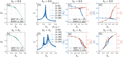
Figure 7: Comparison of ground state energy density and expectation values of local Hamiltonian terms from iPEPS and QMC. (a) Ground state energy density along $h_{x}=0.3$, the legend shows the bond dimensions $(D,\chi)$ of iPEPS and the system size of the QMC. (b) Correlation length from iPEPS with various bond dimensions along $h_{x}=0.3$. (c) Expectation values of $A_{v}$ and $B_{p}$ along $h_{x}=0.3$. (d) Expectation values of $X$ and $Z$ along $h_{x}=0.3$. (e) Ground state energy density along the self-dual line $h_{x}=h_{z}$. (f) Correlation length from iPEPS with various bond dimensions along the self-dual line. (g) Expectation values of $A_{v}$ and $B_{p}$ along the self-dual line line. (h) Expectation values of $X$ and $Z$ along the self-dual line.

We benchmark the ground state energy density and the expectation values of local terms of the toric code model. First, we consider the line $h_{x}=0.3$. The results obtained from iPEPS match perfectly with those from the quantum Monte Carlo (QMC) [21], as shown in Figs. 7a, c and d. Extrapolating the peak positions of correlation length $h^{(J)}_{zc}(D)$ (see Fig. 7b) obtained from the iPEPS with different bond dimensions using a function $h^{(J)}_{zc}(D)=a/D^{b}-h^{(J)}_{zc}$, where we ignore the $\chi$ dependence and $a,b$ are parameters, we can roughly determine that the phase transition point $J$ shown in Fig. 1a is $h^{(J)}_{zc}=0.335(1)$, which is close to result $h^{(J)}_{zc}=0.333(1)$ of Ref. [21].

In Figs. 7e, g and h, we compare the energy density and expectation values along the self-dual line $(h_{x}=h_{z})$ with the QMC result. The correlation length shown in the inset of Fig. 7f has two peaks corresponding to the multi-critical point $M$ and the critical endpoint $K$. Different from finite size QMC simulation where the symmetries can not be broken spontaneously, we can obtain $\langle A_{v}\rangle\neq\langle B_{p}\rangle$ and $\langle X\rangle\neq\langle Z\rangle$ for intermediate fields from the iPEPS results, implying a spontaneous duality symmetry breaking. Using the same method for extrapolating the position of $J$, we can roughly determine that the multi-critical point $M$ shown in Fig. 1a is $h^{(M)}_{zc}=0.3397(2)$, which is close to $h^{(M)}_{zc}=0.340(2)$ of Ref.[21] and $h^{(M)}_{zc}=0.3406(4)$ of Ref. [22]. Moreover, the position of the critical endpoint $K$ strongly depends on the bond dimension $D$. As shown in the inset of Fig. 8b, the extrapolated position of $K$ is $h_{zc}^{(K)}=0.421(2)$, which is close to $h_{zc}^{(K)}=0.418(2)$ of Ref. [21] and indicates that $h_{zc}^{(K)}=0.48(2)$ obtained in Ref. [22] is questionable.

It is natural to expect that the phase transition at the critical endpoint $K$ is also described by the 3D Ising universality class according to the universality hypothesis [22, 17], because it is a conventional spontaneous $\mathbb{Z}_{2}$ symmetry breaking phase transition in $(2+1)$D. It is interesting to check the universality hypothesis using the iPEPS simulation results. Using the same method for extracting other critical exponents, we obtain $\beta_{\text{local}}=0.31(8)$ defined by $|\langle X-Z\rangle|\sim(h_{zc}^{(K)}-h_{z})^{\beta_{\text{local}}}$, as shown in the inset of Fig. 8a; since extrapolated results have large fluctuation, we also show $|\langle X-Z\rangle|$ from iPEPS with bound dimensions $(5,270)$. So $\beta_{\text{local}}=0.31(8)$ is close to $\beta=0.326418(2)$ from the 3D Ising universality class [29]. Moreover, it can be found that the data from $D>3$ can collapse; see Fig. 8b. These results imply that the critical endpoint $K$ is consistent with the 3D Ising universality class.

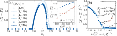
Figure 8: Local order parameter along the self-dual line $(h_{x}=h_{z})$ and its scaling near the critical endpoint $K$. (a) Result from iPEPS with various bond dimensions. Inset: Double-log plot extracting the critical exponent $\beta_{\text{local}}$ of $|\langle X-Z\rangle|$ by a linearly extrapolation in $1/D$ (red dots), where $h^{(F)}_{zc}=0.421(2)$. The blue stars are $|\langle X-Z\rangle|$ from iPEPS with the bond dimensions $(D,\chi)=(5,270)$. (b) Data collapse of the local order parameter at the critical endpoint $K$, where $\nu=0.629970(4)$ and $\beta=0.326418(2)$. Inset: extrapolating the position of the critical end point $K$ from the peak positions of the correlation length in Fig. 7f.

Appendix D Calculation of the FM string order parameter using tensor network methods

In this section, we first discuss the issues one should take care of when evaluating the FM string order parameter whose denominator is defined using a non-contractible loop $L_{x}$. Then, we show the tensor network calculation of the FM string order parameter in the limit of the length of the string $L_{x,1/2}$ being infinite.

When the denominator of the FM string order parameter is defined using a non-contractible loop, it depends on how we choose the degenerate ground states in the toric code phase. For simplicity, let us consider the toric code fixed point $h_{x}=h_{z}=0$, if we use the ground state $\ket{+_{x}+_{y}}$ of Eq. (7) satisfying $W^{X}_{x}\ket{+_{x}+_{y}}=W^{X}_{y}\ket{+_{x}+_{y}}=\ket{+_{x}+_{y}}$, the denominator of the FM string order parameter vanishes: $\bra{+_{x}+_{y}}W_{x}^{Z}\ket{+_{x}+_{y}}=\bra{+_{x}+_{y}}\ket{+_{x}-_{y}}=0$ because $\{W^{Z}_{x},W^{X}_{y}\}=0$, and the FM string order parameter is ill-defined. To fix this problem, we can select the ground state $\ket{0_{x}0_{y}}$ of Eq. (8) such that $\bra{0_{x}0_{y}}W^{x}_{Z}\ket{0_{x}0_{y}}=1$ and then the FM string order parameter is always well-defined. However, if we consider the dual FM string order parameter,

$$O_{X}=\lim_{|\hat{L}_{x,1/2}|\rightarrow\infty}\sqrt{|C_{X}(|\hat{L}_{x,1/2}|)|},\quad\quad C_{X}(|\hat{L}_{x,1/2}|)=\frac{\langle{\Psi}|\prod_{e\in\hat{L}_{x,1/2}}X_{e}|{\Psi}\rangle/\innerproduct{\Psi}{\Psi}}{\sqrt{\bra{\Psi}\prod_{e\in\hat{L}_{x}}X_{e}\ket{\Psi}/\innerproduct{\Psi}{\Psi}}},$$ (10)

where $\hat{L}_{x}$ is a non-contractible loop on the dual lattice whose length is twice the length of the string $\hat{L}_{x,1/2}$ on the dual lattice, and $|\hat{L}_{x,1/2}|$ is the length of the string $\hat{L}_{x,1/2}$, the denominator of the dual FM string order parameter is $\bra{0_{x}0_{y}}W^{X}_{x}\ket{0_{x}0_{y}}=\bra{0_{x}0_{y}}\ket{0_{x}1_{y}}=0$; so the dual FM string order parameter is ill-defined. If we want both the FM string order parameter and its dual to be well-defined simultaneously, we can use the MES $\ket{\boldsymbol{\alpha}}$ shown in Eq. (9), where $\boldsymbol{\alpha}=\boldsymbol{1},\boldsymbol{e},\boldsymbol{m}$ and $\boldsymbol{f}$. Because the denominator $\bra{\boldsymbol{\alpha}}W_{x}^{X}\ket{\boldsymbol{\alpha}}=\pm 1$ and $\bra{\boldsymbol{\alpha}}W_{x}^{Z}\ket{\boldsymbol{\alpha}}=\pm 1$, the FM string order parameter is well defined. In summary, when we only calculate the FM string order parameter $O_{Z}$ ($O_{X}$), we can use the ground state $\ket{0_{x}0_{y}}$ ($\ket{+_{x}+_{y}}$); when considering both $O_{Z}$ and $O_{X}$, we should select the MES. Away from the fixed point ($h_{x}\neq 0$, $h_{z}\neq 0$), we can still follow this rule to select a ground state and evaluate the FM string order parameter and its dual. The results in the main text are evaluated using the ground state $\ket{0_{x}0_{y}}$.

Next, we show how to calculate the FM string order parameter directly in the limit $r=|L_{x,1/2}|\rightarrow\infty$. Using the iPEPS transfer matrices $\mathbb{T}$ and $\mathbb{T}_{Z}$ shown in Fig. 2b of the main text, the FM string order parameter can be expressed as:

$$O_{Z}=\sqrt{\lim_{r\rightarrow\infty}C_{Z}(r)}=\left[\lim_{r\rightarrow\infty}\frac{\Tr(\mathbb{T}^{r}\mathbb{T}^{r}_{Z})/\Tr(\mathbb{T}^{2r})}{\sqrt{\Tr(\mathbb{T}_{Z}^{2r})/\Tr(\mathbb{T}^{2r})}}\right]^{\frac{1}{2}}=\left[\lim_{r\rightarrow\infty}\frac{\Tr(\mathcal{T}^{r}\mathcal{T}^{r}_{Z})/\Tr(\mathcal{T}^{2r})}{\sqrt{\Tr(\mathcal{T}_{Z}^{2r})/\Tr(\mathcal{T}^{2r})}}\right]^{\frac{1}{2}},$$ (11)

where we compress $\mathbb{T}$ and $\mathbb{T}_{Z}$ to transfer matrices $\mathcal{T}$ and $\mathcal{T}_{Z}$ with a dimension $D^{2}\chi^{2}$ using the edge tensors from the CTMRG:

$$\mathcal{T}=\vbox{\hbox{ \includegraphics{mathcal_T.pdf}}},\quad\mathcal{T}_{Z}=\vbox{\hbox{ \includegraphics{mathcal_T_Z.pdf}}}.$$ (12)

We can express $\mathcal{T}$ and $\mathcal{T}_{Z}$ in terms of their eigenvalues and eigenvectors:

$$\mathcal{T}=\sum_{i,\alpha_{i}}t_{i}|V_{i,\alpha_{i}}\rangle\langle V_{i,\alpha_{i}}|,\quad\mathcal{T}_{Z}=\sum_{i,\alpha_{i}}t_{Z,i}|V_{Z,i,\alpha_{i}}\rangle\langle V_{Z,i,\alpha_{i}}|,$$ (13)

where the eigenvectors $\{t_{i}\}$ ($\{t_{Z,i}\}$) are sorted in descending order and $\alpha_{i}$ specifies the degenerate eigenvectors with the same eigenvalue $t_{i}$. In the limit $r\rightarrow\infty$, $\mathcal{T}^{r}$ ($\mathcal{T}^{r}_{Z}$) can be expressed as:

$$\mathcal{T}^{\infty}=\sum_{\alpha_{1}=1}^{d}t_{1}^{\infty}\ket{V_{1,\alpha_{1}}}\bra{V_{1,\alpha_{1}}},\quad\mathcal{T}^{\infty}_{Z}=\sum_{\alpha_{1}=1}^{d_{Z}}t_{Z,1}^{\infty}\ket{V_{Z,1,\alpha_{1}}}\bra{V_{Z,1,\alpha_{1}}},$$ (14)

where $d$ ($d_{Z}$) denotes the number of the dominant eigenvectors of $\mathcal{T}$ and $\mathcal{T}_{Z}$. Therefore, the FM string order parameter can be simplified as:

$$O_{Z}=\left[\lim_{r\rightarrow\infty}\frac{t_{1}^{r}t_{1,Z}^{r}\Tr\left(\sum_{\alpha_{1}=1,\beta_{1}=1}^{d,d_{Z}}\ket{V_{1,\alpha_{1}}}\bra{V_{1,\alpha_{1}}}\ket{V_{Z,1,\beta_{1}}}\bra{V_{Z,1,\beta_{1}}}\right)/\left(dt_{1}^{2r}\right)}{\sqrt{(d_{Z}/d)(t^{2r}_{Z,1}/t_{1}^{2r}})}\right]^{\frac{1}{2}}=\left[\frac{1}{\sqrt{dd_{Z}}}\Tr\left(\sum^{d,d_{Z}}_{\alpha_{1}=1,\beta_{1}=1}\ket{V_{1,\alpha_{1}}}\bra{V_{1,\alpha_{1}}}\ket{V_{Z,\beta_{1}}}\bra{V_{Z,\beta_{1}}}\right)\right]^{\frac{1}{2}}.$$ (15)

When using the ground state $\ket{0_{x}0_{y}}$, we find that $d_{Z}=d=1$ along $h_{x}=0.3$ and the FM string order parameter is simplified to:

$$O_{Z}=\left[\Tr\left(\ket{V_{1}}\bra{V_{1}}\ket{V_{Z,1}}\bra{V_{Z,1}}\right)\right]^{\frac{1}{2}}=|\bra{V_{1}}\ket{V_{Z,1}}|,$$ (16)

where we drop the indices specifying the degeneracy.

The method for calculating $O_{Z}$ can also be used to calculate the dual FM string order parameter $O_{X}$ by constructing a transfer matrix $\mathcal{T}_{X}$, which can be obtained by replacing the $Z$ in $\mathcal{T}_{Z}$ with $X$. When using the ground state is $\ket{0_{x}0_{y}}$, which spontaneously breaks the dual emergent Wison loop symmetry, the FM string order parameter $O_{Z}$ is zero, but the dual one $O_{X}$ is unstable and non-zero, as shown in Fig. 9. However, when we use the MES $\ket{\boldsymbol{1}}$, where both emergent Wilson loop symmetry and its dual do not break, both $O_{X}$ and $O_{Z}$ become zero, see inset of Fig. 9. When using the trivial MES $\ket{\boldsymbol{1}}$ to evaluate the FM string order parameter, the degeneracies $d_{Z}$, $d_{X}$ (degeneracy of the dominant eigenvalue of $\mathcal{T}_{X}$) and $d$ becomes 2, we can use Eq. (15) and its dual version to calculate both $O_{X}$ and $O_{Z}$.

In the trivial phase, if we calculate $O_{Z}$ in the flux condensation region (near and along the $h_{x}$ axis), the results become unstable, which means that $O_{Z}$ evaluated using a set of iPEPS with very closed energies are significantly different. The reason is that along the $h_{x}$ axis ($h_{z}=0$), the denominator of $O_{Z}$ decays exponentially with the area surrounded by the loop $L$ instead of the perimeter of $L$, indicating that the perimeter law coefficient $\alpha_{Z}=-\log(t_{Z,1}/t_{1})=+\infty$ and $t_{Z,1}=0$, so $\mathcal{T}_{Z}=0$. However, it is very difficult to numerically obtain $\mathcal{T}_{Z}=0$, and it doesn’t make sense to calculate $O_{Z}$ using the eigenvectors of $\mathcal{T}_{Z}$, which should be a zero matrix. When not far away from $h_{x}$ axis, the denominator $O_{Z}$ satisfies the perimeter law with a large perimeter law coefficient $\alpha_{Z}=-\log(t_{Z,1}/t_{1})$, which means that $t_{Z,1}$ is very small compared to $t_{1}$ and is the origin of the numerical instability. In contrast, in the charge condensation region (near and along the $h_{z}$ axis), the denominator of $O_{Z}$ satisfies zero law ($\alpha_{Z}=0$, $t=t_{Z}$) along the $h_{z}$ axis ($h_{x}=0$). Near the $h_{z}$ axis, the denominator of $O_{Z}$ satisfies the perimeter law with a small coefficient $\alpha_{Z}$, and $t_{Z,1}$ is very close to $t_{1}$. Therefore, the iPEPS evaluation of $O_{Z}$ is stable in the charge condensation region.

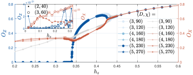
Figure 9: FM string order parameter and its dual along the self-dual line $(h_{x}=h_{z})$. Result from iPEPS $\ket{0_{x}0_{y}}$ with various bond dimensions. Toric code phase, the symmetry breaking phase and the trivial phase are from left to right. $O_{X}$ is not zero in the toric code phase, because ground state is not MES. Inset: we evaluating both the FM string order parameter and its dual using MES $\ket{\boldsymbol{1}}$ both of them become zero (to machine precision) in the toric code phase.

Appendix E Equivalence between the FM string order parameters defined using contractible and non-contractible loops

In this section, we show that the FM string order parameters defined using a non-contractible loop $L_{x}$ and evaluated using the MES $\ket{\boldsymbol{1}}$ and the one defined using a contractible loop $L$ are equivalent, provided that the strings are infinitely long and the ground state is an iPEPS. First, consider the case with a contractible loop. According to Eq. (3) in the main text, we need to consider the following three infinitely large tensor networks:

$$\vbox{\hbox{ \includegraphics{Three_tns.pdf}}},$$ (17)

where the length of the loop and the string are $|L|=4l+4$ and $|L_{1/2}|=2l+2$, respectively. When $l$ is very large, using the edge tensors from the CTMRG, one can replace the middle part with the object shown on the right hand side of the following equation:

$$\vbox{\hbox{ \includegraphics{middle_part.pdf}}},$$ (18)

where the corner tensors (not CTMRG corner tensor) represented by circles can be obtained using a method shown in Ref. [14]. However, we do not need to calculate the corner tensors represented by circles because they will be canceled later. Since the iPEPS tensors have the virtual $\mathbb{Z}_{2}$ symmetry shown in Fig. 5, the right hand side of Eq. (18) should also have this symmetry:

$$\vbox{\hbox{ \includegraphics{sym_middle_part.pdf}}}.$$ (19)

Notice it is not always guaranteed that the object on the right side of Eq. (18) has the virtual $\mathbb{Z}_{2}$ symmetry because the environment of the iPEPS could spontaneously break the virtual $\mathbb{Z}_{2}$ symmetry [50]. If so, we must apply a projector $(\mathbbm{1}^{\otimes N}+Z_{D}^{\otimes N})/2$ to the object to restore the virtual $\mathbb{Z}_{2}$ symmetry, similar to what we do for obtaining the MES $\ket{\boldsymbol{1}}$ [69, 70]. With the object in the right side of Eq. (18) as well as the corner and edge tensors of the CTMRG environment, the three infinity tensor networks in Eq. (17) can be approximated as:

$$\vbox{\hbox{ \includegraphics{Three_tns_approx.pdf}}}.$$ (20)

Because $l$ is very large, we can use Eq. (14) to simplify the three tensor networks in Eq. (20):

$$\vbox{\hbox{ \includegraphics{Three_tns_approx_2.pdf}}},$$ (21)

where we assume that the dominant eigenvectors are not degenerate. We denote the corner objects as

$$\vbox{\hbox{ \includegraphics{C_1.pdf}}}=\vbox{\hbox{ \includegraphics{C_2.pdf}}}=\mathcal{C},\quad\vbox{\hbox{ \includegraphics{C_Z.pdf}}}=\vbox{\hbox{ \includegraphics{C_Z_2.pdf}}}=\mathcal{C}_{Z},$$ (22)

where the symmetry of the square lattice is taken into consideration. With Eqs. (21) and (22), we can express the FM string order parameter as

$$O_{Z}=\left(\frac{t_{1}^{2l}t^{2l}_{Z,1}\mathcal{C}^{2}\mathcal{C}^{2}_{Z}|\innerproduct{V_{Z}}{V}|^{2}/(\mathcal{C}^{4}t_{1}^{4l})}{\sqrt{(\mathcal{C}^{4}_{Z}t_{1,Z}^{4l})/(\mathcal{C}^{4}t_{1}^{4l})}}\right)^{1/2}=\left(\frac{t_{1}^{2l}t^{2l}_{Z,1}\mathcal{C}^{2}\mathcal{C}_{Z}^{2}|\innerproduct{V_{Z}}{V}|^{2}}{\mathcal{C}^{2}_{Z}\mathcal{C}^{2}t_{1,Z}^{2l}t_{1}^{2l}}\right)^{1/2}=|\innerproduct{V_{Z}}{V}|.$$ (23)

Comparing with Eq. (16), we can conclude that the FM string order parameters whose denominators are defined using a non-contractible loop and evaluated using the MES $\ket{\boldsymbol{1}}$ and the one defined using a contractible loop are equivalent in the limit $|L_{1/2}|\rightarrow\infty$. When the symmetry shown in Eq. (19) is not satisfied, we should take all four diagrams in Eq. (19) into consideration, and there are degenerate dominant eigenvectors so that Eq. (21) is not valid. Using the virtual $\mathbb{Z}_{2}$ symmetry of the iPEPS tensor and the condition shown in Eq. (32), we can still arrive at the same conclusion. And we do not show the more complicated case for simplicity.

Appendix F FM string order parameter for the deformed toric code state

In order to study the topological phase transitions of the toric code model without solving the ground states of the toric code model, a deformed toric code state has been considered [50, 51, 52], whose phase diagram is similar to that of the toric code model. An interesting question is if we can use the FM string order parameter to characterize the phase transitions of the deformed toric code state. Because the deformed state has an analytical expression, we can obtain physical pictures from the deformed toric code state to understand the FM string order parameter.

The deformed toric code state is defined as:

$$\ket{\psi(g_{x},g_{z})}=\prod_{e}Q_{e}(g_{x},g_{z})\ket{\text{TC}}=\prod_{e}(1+g_{x}X_{e}+g_{z}Z_{e})\ket{\text{TC}},$$ (24)

where $\ket{\text{TC}}$ is a ground state ( the state $\ket{0_{x}0_{y}}$ in Fig. 6c ) of the Hamiltonian (1) at $h_{x}=h_{z}=0$, and $g_{x}$ and $g_{z}$ are parameters satisfying $g_{x}^{2}+g_{z}^{2}\leq 1$. A phase diagram of the deformed toric code state is shown in Fig. 10a, there are two trivial phases with charge or flux condensation, separately, and they are separated by a KT transition line. The phase transition lines from the toric code phase to the trivial phase belong to the 2D Ising universality class. We calculate the FM string order parameter along $g_{x}=0.14$ by contracting the iPEPS of the deformed toric code state using the boundary infinite matrix product states (iMPS) with various bond dimensions $\chi$, and the result is shown in Fig. 10b. We can extract a critical exponent $\beta_{\text{FM}}$ of the FM string order parameter according to $O_{Z}\sim(g_{z}-g_{zc})^{\beta_{\text{FM}}}$, where we numerically determine the critical point $g_{zc}=0.2227(3)$ and extrapolate $O_{Z}$ using different iMPS bond dimensions $\chi$. The extracted $\beta_{\text{FM}}=0.117(5)$ is close to the $\beta=1/8=0.125$ from the 2D Ising universality class. To double-check, we also apply the data collapse method shown in Ref. [71] to the FM string order parameter in Fig. 10c. These results indicate that the scaling behavior of the FM string order parameter near and at the critical line of the deformed toric code state is controlled by the 2D Ising universality class.

Figure 10: FM string order parameter for the deformed TC state. (a) The phase diagram of the deformed TC state shown in Eq. (24). (b) The FM string order parameter along $g_{x}=0.14$ [the horizontal dash line in (a)], calculated using iMPS with various bond dimensions $\chi$. Inset, extract the critical exponent $\beta_{\text{FM}}$ from the FM string order parameter, which $O_{Z}$ is obtained via extrapolating different $\chi$. (c) Data collapse of the FM string order parameter, where $g_{zc}=0.2227(3)$, $\beta=1/8$ and $\nu=1$. (d) Finite and infinite FM string order parameter calculated along $g_{x}^{2}+g_{z}^{2}=0.65^{2}$ [dash quarter circle in (a)] from the iMPS with the bond dimension $\chi=20$, where $\theta=\arctan(g_{x}/g_{z})$. The legend shows the size of the area surrounded by the loop operator displayed in Eq. (17).

Unlike the variationally optimized iPEPS, it is numerically stable to calculate the FM string order parameter in the flux condensation phase of the deformed toric code state shown in Eq. (24). One reason for this is that the iPEPS of the deformed toric code state is not variational. Another possible reason is that the expectation value of the Wilson loop operator evaluated from the deformed toric code state always satisfies perimeter law even along the $g_{x}$ axis ($g_{z}=0$) in the flux condensation phase  [72]. In contrast, the expectation value of the Wilson loop operator evaluated using the ground state of the toric code model along the $h_{x}$ axis ($h_{z}=0$) satisfies the area law. We calculate the FM string order parameter with an infinite string length $|L_{1/2}|$ along a path $g^{2}_{x}+g^{2}_{z}=0.65^{2}$, as shown in Fig. 10d. Surprisingly, we find that the FM string order parameter can be discontinuous at $\theta\approx 0.4\pi$ even if there is no bulk phase transition. In order to exclude the possibility that there are some artifacts of our method that cause the discontinuity, we also evaluate the FM string order parameter with some finite string length $r=|L_{1/2}|$ in Fig. 10d, which indeed implies that the FM string order parameter becomes discontinuous with $r\rightarrow\infty$.

Next, let us talk about the relation between the FM string order parameter and the virtual order parameter defined for a topological iPEPS [52] and the origin of the discontinuity of the FM string order parameter without bulk phase transition in Fig. 10d. At first, let us review the definition of the virtual order parameter. For a fixed point ground state, we can create a pair of charge excitations at the vertices $v$ and $v^{\prime}$ by inserting two $Z$ operators at the virtual level, because it is equivalent to $Z$ operators along the string $L_{1/2}$ on the physical level:

$$\ket{\boldsymbol{e}_{v},\boldsymbol{e}_{v^{\prime}}}=\vbox{\hbox{ \includegraphics{virtual_string.pdf}}}=\vbox{\hbox{ \includegraphics{physical_string.pdf}}}.$$ (25)

Then, the virtual order parameter can be expressed as

$$O_{Z}^{(\text{virtual})}=\lim_{|L_{1/2}|\rightarrow\infty}\left(\frac{\bra{\text{TC}}\prod_{e}Q_{e}^{2}(g_{x},g_{z})\ket{\boldsymbol{e}_{v},\boldsymbol{e}_{v^{\prime}}}}{\bra{\text{TC}}\prod_{e}Q_{e}^{2}(g_{x},g_{z})\ket{\text{TC}}}\right)^{1/2}.$$ (26)

In contrast, the FM string order parameter can be expressed as

$$O_{Z} =\lim_{|L_{L/2}|\rightarrow\infty}\left\{\frac{\bra{\text{TC}}\left[\prod_{e}Q_{e}(g_{x},g_{z})\right]\left(\prod_{e\in L_{1/2}}Z_{e}\right)\left(\prod_{e}Q_{e}(g_{x},g_{z})\right]\ket{\text{TC}}}{\sqrt{\bra{\text{TC}}\left[\prod_{e}Q_{e}(g_{x},g_{z})\right]\left(\prod_{e\in L}Z_{e}\right)\left[\prod_{e}Q_{e}(g_{x},g_{z})\right]\ket{\text{TC}}}}\right\}^{1/2}$$

$$=\lim_{|L_{1/2}|\rightarrow\infty}\left\{\frac{\bra{\text{TC}}\left[\prod_{e}Q_{e}(g_{x},g_{z})\right]\left[\prod_{e\in L_{1/2}}Q_{e}(g_{x},g_{z})Q_{e}(-g_{x},g_{z})\right]\ket{\boldsymbol{e}_{v},\boldsymbol{e}_{v^{\prime}}}}{\sqrt{\bra{\text{TC}}\left[\prod_{e\notin L}Q^{2}_{e}(g_{x},g_{z})\right]\left[\prod_{e\in L}Q_{e}(g_{x},g_{z})Q_{e}(-g_{x},g_{z})\right]\ket{\text{TC}}}}\right\}^{1/2}.$$ (27)

When $g_{x}=0$, the FM string order parameter and the virtual order parameter are equal: $O_{Z}=O^{\text{(virtual)}}_{Z}$. When $g_{x}\neq 0$, the FM string order parameter has extra defect lines along the string $L_{1/2}$ in the numerator and the loop $L$ in the denominator compared to the virtual order parameter. If $g_{x}$ is not too large, the string operator $\prod_{e\in L_{1/2}}Z_{e}$ creates two charges at its two ends when applied to the deformed toric code state, so the FM string order parameter and the virtual order parameter are quantitatively the same and we say that the FM string order parameter detects the condensation of charges. However, if $g_{x}$ is too large, the string operator $\prod_{e\in L_{1/2}}Z_{e}$ fails to create the charges when applied to the deformed toric code state, and the FM string order parameter becomes essentially different from the virtual order parameter.

We can understand when the string operator $\prod_{e\in L_{1/2}}Z_{e}$ fails to create charges from transfer matrices:

$$\mathcal{T}_{Q^{2}}=\vbox{\hbox{ \includegraphics[width=60.6045pt]{T_QQ.pdf}}},\quad\mathcal{T}_{Q\tilde{Q}}=\vbox{\hbox{ \includegraphics[width=60.6045pt]{T_QQ2.pdf}}},$$ (28)

where

$$\vbox{\hbox{ \includegraphics[width=47.60158pt]{Q2_blue_1.pdf}}}=\vbox{\hbox{ \includegraphics[width=30.33046pt]{Q2_blue_2.pdf}}},\quad\vbox{\hbox{ \includegraphics[width=47.60158pt]{Q2_yellow_1.pdf}}}=\vbox{\hbox{ \includegraphics[width=30.33046pt]{Q2_yellow_2.pdf}}},\quad\vbox{\hbox{ \includegraphics[width=47.60158pt]{QQ2_blue_1.pdf}}}=\vbox{\hbox{ \includegraphics[width=30.33046pt]{QQ2_blue_2.pdf}}},\quad\vbox{\hbox{ \includegraphics[width=47.60158pt]{QQ2_yellow_1.pdf}}}=\vbox{\hbox{ \includegraphics[width=30.33046pt]{QQ2_yellow_2.pdf}}},$$ (29)

$\tilde{Q}(g_{x},g_{z})=-Q(g_{x},g_{z})$, and $E_{Q}$ is the boundary MPS tensor of the double tensor labeled by $Q^{2}$. Notice that the black and white dot tensors are defined in Fig. 5a. Using the method shown in Sec. D, the virtual order parameter and FM string order parameter can be expressed as

$$O_{Z}^{(\text{virtual})}=\vbox{\hbox{ \includegraphics[width=42.5085pt]{O_Z.pdf}}},\quad O_{Z}=\vbox{\hbox{ \includegraphics[width=42.5085pt]{O_Z_FM.pdf}}},$$ (30)

where $V$ and $\tilde{V}$ are fixed points of $\mathcal{T}_{Q^{2}}$ and $\mathcal{T}_{Q\tilde{Q}}$, respectively. Because $\mathcal{T}_{Q^{2}}$ and $\mathcal{T}_{Q\tilde{Q}}$ has a $\mathbb{Z}_{2}$ symmetry $U_{X}\otimes X\otimes X\otimes U_{X}$ in the toric code phase and the flux condensation phase (this symmetry doesn’t exist in the charge condensation phase because the boundary MPS generated by $E_{Q}$ spontaneously breaks the virtual $\mathbb{Z}_{2}$ symmetry [50]):

$$\vbox{\hbox{ \includegraphics[width=60.6045pt]{T_QQ.pdf}}}=\vbox{\hbox{ \includegraphics[width=77.10715pt]{T_QQ_sym.pdf}}},\quad\vbox{\hbox{ \includegraphics[width=60.6045pt]{T_QQ2.pdf}}}=\vbox{\hbox{ \includegraphics[width=77.10715pt]{T_QQ2_sym.pdf}}}.$$ (31)

where $U_{X}$ is a $\chi\times\chi$ matrix defined via

$$\vbox{\hbox{\includegraphics[width=60.6045pt]{MPS_theorem_1.pdf}}}=\vbox{\hbox{ \includegraphics[width=77.10715pt]{MPS_theorem_2.pdf}}},$$ (32)

we say the parity of $V$ and $\tilde{V}$ is even (odd) if they are eigenstates of $U_{X}\otimes X\otimes X\otimes U_{X}$ with eigenvalues 1 (-1). It can be checked that $V$ is always parity even in the toric code phase and the flux condensation phase, so $O^{\text{(virtual)}}_{Z}=0$ because of Eq. (30) and $\{U_{X}\otimes X\otimes X\otimes U_{X},\mathbbm{1}_{\chi}\otimes Z\otimes\mathbbm{1}_{2}\otimes\mathbbm{1}_{\chi}\}=0$. However, along to $g_{x}^{2}+g_{z}^{2}=0.65^{2}$ shown in Figs. 10a and d, $\tilde{V}$ is parity even (odd) when $\theta\gtrsim 0.4\pi$ ($0.25\pi<\theta\lesssim 0.4\pi$), so $O_{Z}=0$ ($O_{Z}\neq 0$) when $\theta\gtrsim 0.4\pi$ ($0.25\pi<\theta\lesssim 0.4\pi$) according to Eq. (30). Therefore, in the flux condensed phase, the abrupt change of parity of $\tilde{V}$ is the origin of the discontinuity observed in Fig. 10d.

From the results of the deformed toric code state and the results from the toric code model, we conjecture that it only makes sense to apply the FM string order parameter to the toric code phase and charge condensation phase/region, and a common feature of charge condensation region/phase is that there is an emergent non-contractible Wilson loop symmetry. First, let us consider the deformed toric code state, since charges are confined (deconfined) in the flux condensation phase (the toric code phase and the charge condensation phase) of the deformed toric code state (24), so if we first apply a non-contractible loop $L_{x}$ of $Z$, which can be interpreted as an electric line, on $\ket{\text{TC}}$ and then apply the deformation $\prod_{e}Q_{e}(g_{x},g_{z})$, the norm of the obtained state is

$$\lim_{|L_{x}|\rightarrow\infty}\bra{\text{TC}}\left(\prod_{e\in L_{x}}Z_{e}\right)\left[\prod_{e}Q^{2}_{e}(g_{x},g_{z})\right]\left(\prod_{e\in L_{x}}Z_{e}\right)\ket{\text{TC}}=\begin{cases}0,&\text{flux condensation phase;}\\ \bra{\text{TC}}\prod_{e}Q^{2}_{e}(g_{x},g_{z})\ket{\text{TC}},&\text{toric code and charge condensation phases.}\end{cases}$$ (33)

So in the toric code phase and the charge condensation phase we have

$$\ket{\psi(g_{x},g_{z})}=\left[\prod_{e}Q_{e}(g_{x},g_{z})\right]\ket{\text{TC}}=\left[\prod_{e}Q_{e}(g_{x},g_{z})\right]\left(\prod_{e\in L_{x}}Z_{e}\right)\ket{\text{TC}},$$ (34)

and there is an “emergent” (non-contractible) Wilson loop symmetry $\tilde{W}^{Z}_{x}$ in the toric code phase and the charge condensation phase:

$$\ket{\psi(g_{x},g_{z})}=\left(\prod_{e\in L_{x}}Z_{e}Q_{e}(-g_{x},g_{z})Q_{e}^{-1}(g_{x},g_{z})\right]\left[\prod_{e}Q_{e}(g_{x},g_{z})\right]\ket{\text{TC}}=\left(\prod_{e\in L_{x}}Z_{e}Q_{e}(-g_{x},g_{z})Q_{e}^{-1}(g_{x},g_{z})\right)\ket{\psi(g_{x},g_{z})}=\tilde{W}^{Z}_{x}\ket{\psi(g_{x},g_{z})},$$ (35)

notice that $Q_{e}^{-1}$ exists when $g_{x}^{2}+g_{z}^{2}<1$ and $\left(\tilde{W}^{Z}_{x}\right)^{2}=1$. However, there is no “emergent” (non-contractible) Wilson loop symmetry in the flux condensation phase because Eq. (34) is not valid.

Then let us consider the Hamiltonian case, there is no phase transition between the flux condensation region and the charge condensation region, see Fig. 1a of the main text. A scenario proposed in Ref. [17] can help us determine the boundary of the charge (flux) condensation region. On the $h_{z}$ axis ($h_{x}=0$), the toric code model has the Wilson loop symmetry $\prod_{e\in L}Z_{e}$. Slightly away from $h_{z}$ axis, the explicit Wilson loop operator $\prod_{e\in L}Z_{e}$ is no longer a symmetry, but there is an implicit emergent Wilson loop symmetry [30, 24, 31]. Far from the $h_{z}$ axis, the trivial phase has no emergent Wilson loop symmetry. It has been proposed that a percolation transition (not phase transition) separates the regions with and without emergent 1-form Wilson loop symmetry in the trivial phase [17]. Since the charges are created at the endpoints of a string operator obtained by opening an emergent Wilson loop operator, we can not create (deconfined) charges in the region where there is no emergent Wilson loop symmetry. So it is conceivable that the boundary of the charge condensation region in the trivial phase is determined by the percolation transition. Since it is numerically unstable to calculate the FM string order parameter in the flux condensation region of the toric code model, and the FM string order parameter is discontinuous in the flux condensation phase of the deformed toric code state (see Fig. 10d), we conjecture that (i) the FM string order parameter loses its meaning in the region without emergent Wilson loop symmetry; (ii) in the charge condensation region where emergent Wilson loop symmetry does not break the FM string order parameter is non-zero, (iii) in the toric code phase where the emergent Wilson loop symmetry breaks spontaneously, the FM string order parameter is zero.

References

- Tsui et al. [1982] D. C. Tsui, H. L. Stormer, and A. C. Gossard, Two-dimensional magnetotransport in the extreme quantum limit, Phys. Rev. Lett. 48, 1559 (1982).
- Laughlin [1983] R. B. Laughlin, Anomalous quantum hall effect: An incompressible quantum fluid with fractionally charged excitations, Phys. Rev. Lett. 50, 1395 (1983).
- Kitaev [2003] A. Kitaev, Fault-tolerant quantum computation by anyons, Annals of Physics 303, 2 (2003).
- Kitaev [2006] A. Kitaev, Anyons in an exactly solved model and beyond, Annals of Physics 321, 2 (2006), january Special Issue.
- Levin and Wen [2005] M. A. Levin and X.-G. Wen, String-net condensation: A physical mechanism for topological phases, Phys. Rev. B 71, 045110 (2005).
- Wen [2015] X.-G. Wen, A theory of 2+1D bosonic topological orders, National Science Review 3, 68 (2015), https://academic.oup.com/nsr/article-pdf/3/1/68/31565649/nwv077.pdf .
- Wen [2017] X.-G. Wen, Colloquium: Zoo of quantum-topological phases of matter, Rev. Mod. Phys. 89, 041004 (2017).
- Satzinger et al. [2021] K. J. Satzinger, Y.-J. Liu, A. Smith, C. Knapp, et al., Realizing topologically ordered states on a quantum processor, Science 374, 1237 (2021), https://www.science.org/doi/pdf/10.1126/science.abi8378 .
- Semeghini et al. [2021] G. Semeghini, H. Levine, A. Keesling, S. Ebadi, T. T. Wang, D. Bluvstein, R. Verresen, H. Pichler, M. Kalinowski, R. Samajdar, A. Omran, S. Sachdev, A. Vishwanath, M. Greiner, V. Vuletić, and M. D. Lukin, Probing topological spin liquids on a programmable quantum simulator, Science 374, 1242 (2021), https://www.science.org/doi/pdf/10.1126/science.abi8794 .
- Iqbal et al. [2023] M. Iqbal, N. Tantivasadakarn, R. Verresen, S. L. Campbell, J. M. Dreiling, C. Figgatt, J. P. Gaebler, J. Johansen, M. Mills, S. A. Moses, J. M. Pino, A. Ransford, M. Rowe, P. Siegfried, R. P. Stutz, M. Foss-Feig, A. Vishwanath, and H. Dreyer, Creation of non-abelian topological order and anyons on a trapped-ion processor (2023), arXiv:2305.03766 [quant-ph] .
- Fredenhagen and Marcu [1983] K. Fredenhagen and M. Marcu, Charged states in z_2 gauge theories, Commun. Math. Phys 92 (1983).
- Marcu [1986] M. Marcu, (uses of) an order parameter for lattice gauge theories with matter fields, Lattice Gauge Theory: A Challenge in Large-Scale Computing , 267 (1986).
- Verresen et al. [2021] R. Verresen, M. D. Lukin, and A. Vishwanath, Prediction of toric code topological order from rydberg blockade, Phys. Rev. X 11, 031005 (2021).
- Vanderstraeten et al. [2016] L. Vanderstraeten, J. Haegeman, P. Corboz, and F. Verstraete, Gradient methods for variational optimization of projected entangled-pair states, Phys. Rev. B 94, 155123 (2016).
- Corboz [2016] P. Corboz, Variational optimization with infinite projected entangled-pair states, Phys. Rev. B 94, 035133 (2016).
- Liao et al. [2019] H.-J. Liao, J.-G. Liu, L. Wang, and T. Xiang, Differentiable programming tensor networks, Phys. Rev. X 9, 031041 (2019).
- Somoza et al. [2021] A. M. Somoza, P. Serna, and A. Nahum, Self-dual criticality in three-dimensional gauge theory with matter, Phys. Rev. X 11, 041008 (2021).
- Bonati et al. [2022] C. Bonati, A. Pelissetto, and E. Vicari, Multicritical point of the three-dimensional gauge higgs model, Phys. Rev. B 105, 165138 (2022).
- Oppenheim et al. [2023] L. Oppenheim, M. Koch-Janusz, S. Gazit, and Z. Ringel, Machine learning the operator content of the critical self-dual ising-higgs gauge model (2023), arXiv:2311.17994 [cond-mat.str-el] .
- Bonati et al. [2024] C. Bonati, A. Pelissetto, and E. Vicari, Comment on ”machine learning the operator content of the critical self-dual ising-higgs gauge model”, arxiv:2311.17994v1 (2024), arXiv:2401.10563 [cond-mat.stat-mech] .
- Wu et al. [2012] F. Wu, Y. Deng, and N. Prokof’ev, Phase diagram of the toric code model in a parallel magnetic field, Phys. Rev. B 85, 195104 (2012).
- Vidal et al. [2009] J. Vidal, S. Dusuel, and K. P. Schmidt, Low-energy effective theory of the toric code model in a parallel magnetic field, Phys. Rev. B 79, 033109 (2009).
- Dusuel et al. [2011] S. Dusuel, M. Kamfor, R. Orús, K. P. Schmidt, and J. Vidal, Robustness of a perturbed topological phase, Phys. Rev. Lett. 106, 107203 (2011).
- Verresen et al. [2022] R. Verresen, U. Borla, A. Vishwanath, S. Moroz, and R. Thorngren, Higgs condensates are symmetry-protected topological phases: I. discrete symmetries (2022), arXiv:2211.01376 [cond-mat.str-el] .
- Wegner [1971] F. J. Wegner, Duality in generalized ising models and phase transitions without local order parameters, Journal of Mathematical Physics 12, 2259 (1971).
- Trebst et al. [2007] S. Trebst, P. Werner, M. Troyer, K. Shtengel, and C. Nayak, Breakdown of a topological phase: Quantum phase transition in a loop gas model with tension, Phys. Rev. Lett. 98, 070602 (2007).
- Blöte and Deng [2002] H. W. J. Blöte and Y. Deng, Cluster monte carlo simulation of the transverse ising model, Phys. Rev. E 66, 066110 (2002).
- Note [1] It is also called Ising* universality class because on a torus toric code model in a longitudinal field is mapped to the transverse field Ising model in even sector, we ignore this difference and still say that the transition cross is D Ising universality class [65].
- Kos et al. [2016] F. Kos, D. Poland, D. Simmons-Duffin, and A. Vichi, Precision islands in the ising and o (n) models, Journal of High Energy Physics 2016, 1 (2016).
- Hastings and Wen [2005] M. B. Hastings and X.-G. Wen, Quasiadiabatic continuation of quantum states: The stability of topological ground-state degeneracy and emergent gauge invariance, Phys. Rev. B 72, 045141 (2005).
- Cong et al. [2023] I. Cong, N. Maskara, M. C. Tran, H. Pichler, G. Semeghini, S. F. Yelin, S. Choi, and M. D. Lukin, Enhancing detection of topological order by local error correction (2023), arXiv:2209.12428 [quant-ph] .
- Pace and Wen [2023] S. D. Pace and X.-G. Wen, Exact emergent higher-form symmetries in bosonic lattice models, Phys. Rev. B 108, 195147 (2023).
- Huse and Leibler [1991] D. A. Huse and S. Leibler, Are sponge phases of membranes experimental gauge-higgs systems?, Phys. Rev. Lett. 66, 437 (1991).
- Cian et al. [2022] Z.-P. Cian, M. Hafezi, and M. Barkeshli, Extracting wilson loop operators and fractional statistics from a single bulk ground state (2022), arXiv:2209.14302 [cond-mat.str-el] .
- Note [2] Notice that should be understood as the length of instead of the distance between its two ends because the bulk of the -string can not be deformed freely when . In addition, for the gauge Higgs model, we should replace the string operator with , where and are two vertices at the ends of the string .
- Zhang et al. [2012] Y. Zhang, T. Grover, A. Turner, M. Oshikawa, and A. Vishwanath, Quasiparticle statistics and braiding from ground-state entanglement, Phys. Rev. B 85, 235151 (2012).
- [37] See Supplemental Material for the technical details about the iPEPS optimization and the topologically degenerate ground states in terms of iPEPS, benchmark iPEPS results uisng the QMC results, calculating FM order parameter using tensor network methods, and the FM order parameters for the deformed wavefunction .
- Crone and Corboz [2020] S. P. G. Crone and P. Corboz, Detecting a topologically ordered phase from unbiased infinite projected entangled-pair state simulations, Phys. Rev. B 101, 115143 (2020).
- Corboz et al. [2018] P. Corboz, P. Czarnik, G. Kapteijns, and L. Tagliacozzo, Finite correlation length scaling with infinite projected entangled-pair states, Phys. Rev. X 8, 031031 (2018).
- Rader and Läuchli [2018] M. Rader and A. M. Läuchli, Finite correlation length scaling in lorentz-invariant gapless ipeps wave functions, Phys. Rev. X 8, 031030 (2018).
- Vanhecke et al. [2022] B. Vanhecke, J. Hasik, F. Verstraete, and L. Vanderstraeten, Scaling hypothesis for projected entangled-pair states, Phys. Rev. Lett. 129, 200601 (2022).
- Iqbal et al. [2018] M. Iqbal, K. Duivenvoorden, and N. Schuch, Study of anyon condensation and topological phase transitions from a topological phase using the projected entangled pair states approach, Phys. Rev. B 97, 195124 (2018).
- Duivenvoorden et al. [2017] K. Duivenvoorden, M. Iqbal, J. Haegeman, F. Verstraete, and N. Schuch, Entanglement phases as holographic duals of anyon condensates, Phys. Rev. B 95, 235119 (2017).
- Xu and Schuch [2021] W.-T. Xu and N. Schuch, Characterization of topological phase transitions from a non-abelian topological state and its galois conjugate through condensation and confinement order parameters, Phys. Rev. B 104, 155119 (2021).
- Xu et al. [2022] W.-T. Xu, J. Garre-Rubio, and N. Schuch, Complete characterization of non-abelian topological phase transitions and detection of anyon splitting with projected entangled pair states, Phys. Rev. B 106, 205139 (2022).
- Iqbal and Schuch [2021] M. Iqbal and N. Schuch, Entanglement order parameters and critical behavior for topological phase transitions and beyond, Phys. Rev. X 11, 041014 (2021).
- Schuch et al. [2010a] N. Schuch, I. Cirac, and D. Pérez-García, Peps as ground states: Degeneracy and topology, Annals of Physics 325, 2153 (2010a).
- Bultinck et al. [2017] N. Bultinck, M. Mariën, D. Williamson, M. Şahinoğlu, J. Haegeman, and F. Verstraete, Anyons and matrix product operator algebras, Annals of Physics 378, 183 (2017).
- Şahinoğlu et al. [2021] M. B. Şahinoğlu, D. Williamson, N. Bultinck, M. Mariën, J. Haegeman, N. Schuch, and F. Verstraete, Characterizing topological order with matrix product operators, in Annales Henri Poincaré, Vol. 22 (Springer, 2021) pp. 563–592.
- Haegeman et al. [2015a] J. Haegeman, V. Zauner, N. Schuch, and F. Verstraete, Shadows of anyons and the entanglement structure of topological phases, Nature communications 6, 8284 (2015a).
- Haegeman et al. [2015b] J. Haegeman, K. Van Acoleyen, N. Schuch, J. I. Cirac, and F. Verstraete, Gauging quantum states: From global to local symmetries in many-body systems, Phys. Rev. X 5, 011024 (2015b).
- Zhu and Zhang [2019] G.-Y. Zhu and G.-M. Zhang, Gapless coulomb state emerging from a self-dual topological tensor-network state, Phys. Rev. Lett. 122, 176401 (2019).
- Kos et al. [2014] F. Kos, D. Poland, and D. Simmons-Duffin, Bootstrapping the o (n) vector models, Journal of High Energy Physics 2014, 1 (2014).
- Chester et al. [2020] S. M. Chester, W. Landry, J. Liu, D. Poland, D. Simmons-Duffin, N. Su, and A. Vichi, Carving out ope space and precise o (2) model critical exponents, Journal of High Energy Physics 2020, 1 (2020).
- Linsel et al. [2024] S. M. Linsel, A. Bohrdt, L. Homeier, L. Pollet, and F. Grusdt, Percolation as a confinement order parameter in lattice gauge theories (2024), arXiv:2401.08770 [quant-ph] .
- Gaiotto et al. [2015] D. Gaiotto, A. Kapustin, N. Seiberg, and B. Willett, Generalized global symmetries, Journal of High Energy Physics 2015, 1 (2015).
- Wen [2019] X.-G. Wen, Emergent anomalous higher symmetries from topological order and from dynamical electromagnetic field in condensed matter systems, Phys. Rev. B 99, 205139 (2019).
- McGreevy [2023] J. McGreevy, Generalized symmetries in condensed matter, Annual Review of Condensed Matter Physics 14, 57 (2023), https://doi.org/10.1146/annurev-conmatphys-040721-021029 .
- [59] The broken emergent 1-from symmetry defined on a non-contractible loop can be restored using minimally entangled states. Also, notice that the emergent Wilson loop symmetry defined on a contractible loop is unbroken for any ground state.
- Gregor et al. [2011] K. Gregor, D. A. Huse, R. Moessner, and S. L. Sondhi, Diagnosing deconfinement and topological order, New Journal of Physics 13, 025009 (2011).
- Xu et al. [2020] W.-T. Xu, Q. Zhang, and G.-M. Zhang, Tensor network approach to phase transitions of a non-abelian topological phase, Phys. Rev. Lett. 124, 130603 (2020).
- Raussendorf et al. [2023] R. Raussendorf, W. Yang, and A. Adhikary, Measurement-based quantum computation in finite one-dimensional systems: string order implies computational power, Quantum 7, 1215 (2023).
- [63] R. Verresen, A. Vishwanath, and N. Schuch, in preparation; see also talk at the 2nd IQTN Plenary Meeting.
- Xu et al. [2024] W.-T. Xu, F. Pollmann, and M. Knap, Critical behavior of the Fredenhagen-Marcu order parameter for topological phase transitions, 10.5281/zenodo.10494400 (2024).
- Schuler et al. [2016] M. Schuler, S. Whitsitt, L.-P. Henry, S. Sachdev, and A. M. Läuchli, Universal signatures of quantum critical points from finite-size torus spectra: A window into the operator content of higher-dimensional conformal field theories, Phys. Rev. Lett. 117, 210401 (2016).
- Francuz et al. [2023] A. Francuz, N. Schuch, and B. Vanhecke, Stable and efficient differentiation of tensor network algorithms (2023), arXiv:2311.11894 [quant-ph] .
- Gu et al. [2008] Z.-C. Gu, M. Levin, and X.-G. Wen, Tensor-entanglement renormalization group approach as a unified method for symmetry breaking and topological phase transitions, Phys. Rev. B 78, 205116 (2008).
- Schuch et al. [2010b] N. Schuch, I. Cirac, and D. Pérez-García, Peps as ground states: Degeneracy and topology, Annals of Physics 325, 2153 (2010b).
- Haller et al. [2023] L. Haller, W.-T. Xu, Y.-J. Liu, and F. Pollmann, Quantum phase transition between symmetry enriched topological phases in tensor-network states, Phys. Rev. Res. 5, 043078 (2023).
- Xu et al. [2023] W.-T. Xu, M. Knap, and F. Pollmann, Entanglement of gauge theories: from the toric code to the lattice gauge higgs model (2023), arXiv:2311.16235 [cond-mat.str-el] .
- Vanhecke et al. [2019] B. Vanhecke, J. Haegeman, K. Van Acoleyen, L. Vanderstraeten, and F. Verstraete, Scaling hypothesis for matrix product states, Phys. Rev. Lett. 123, 250604 (2019).
- Huxford et al. [2023] J. Huxford, D. X. Nguyen, and Y. B. Kim, Gaining insights on anyon condensation and 1-form symmetry breaking across a topological phase transition in a deformed toric code model (2023), arXiv:2305.07063 [cond-mat.str-el] .