Perspectives on locally weighted ensemble Kalman methods

Abstract

This manuscript derives locally weighted ensemble Kalman methods from the point of view of ensemble-based function approximation. This is done by using pointwise evaluations to build up a local linear or quadratic approximation of a function, tapering off the effect of distant particles via local weighting. This introduces a candidate method (the locally weighted Ensemble Kalman method) for combining the strengths of the particle filter (ability to cope with nonlinear maps and non-Gaussian distributions) and the Ensemble Kalman filter (no filter degeneracy), and can also be applied to optimisation and sampling tasks.

Keywords: Ensemble Kalman, Filtering, Inversion, Optimisation, Sampling, Bayesian Inference

MSC class: 62F15, 65N75, 37N40, 90C56

1 Introduction

The following problem motivates the study of Ensemble Kalman methods: Let $\mathcal{X}$ be a Hilbert space, the parameter space and a possibly nonlinear measurement operator $A:\mathcal{X}\to\mathcal{Y}$ into a feature (or observation) space $\mathcal{Y}$. Given an observation $y\in\mathcal{Y}$ from a noisy measurement

$$y=A(u)+\varepsilon,$$ (1)

where $\varepsilon\in\mathcal{Y}$ is a realisation of measurement noise (often assumed to be Gaussian), we want to infer the original parameter $u\in\mathcal{X}$. Often, a misfit functional $\Phi:\mathcal{X}\to\mathbb{R}$ is constructed which associates a cost to a given parameter value. For example, when $\varepsilon\sim\mathcal{N}(0,I)$ is a Gaussian random variable (setting covariance to the identity purely out of convenience),

$$\Phi(u)=\frac{1}{2}\|y-A(u)\|^{2}$$ (2)

This setting is quite general and covers many interesting optimisation, filtering, and sampling problems. For concreteness and in order to exclude a few pathologies of infinite-dimensional spaces (although the Ensemble Kalman method is quite robust in this regard), we will set $\mathcal{X}=\mathbb{R}^{p}$ and $\mathcal{Y}=\mathbb{R}^{d}$.

In this manuscript we will consider in a very general sense the family of Ensemble Kalman methods, which have been developed in the context of filtering first ([Eve03]), based on the Kalman filter (EnKF, [Kal60]), and then applied to inversion/optimisation (EKI, [ILS13]), and sampling (EKS, [Gar+20] and ALDI, [GNR20]), with applications in weather forecasting, geophysics, control, robotics, machine learning, any many others. We refer the reader to [CRS22] for a recent overview and the references therein. We will not attempt to enumerate all relevant or interesting variants which have been established, like the original EnKF, the Ensemble Square Root filter (EnSRF, [Tip+03]), the EKS, the EKI, ALDI, Tikhonov-regularised Ensemble Kalman inversion (TEKI, [CST20]), and countless others, with both discrete-time and continuous time variants, in the deterministic and stochastic or optimal transport setting. Instead, we direct our attention to an adequate “model” Ensemble Kalman method (similar to the EKI). Most results and ideas in this manuscript can then be straightforwardly transferred to the reader’s favorite Ensemble Kalman flavour and application setting.

In this manuscript, when we talk about “the (linear) EK method”, we will mean the following coupled system of $J\in\mathbb{N}$ ordinary differential equations (ODEs).

$$\frac{\mathrm{d}}{\mathrm{d}t}u^{(i)}=-C_{u,A}\cdot\left(A(u^{(i)})-y\right).$$ (3)

This system of equations tracks the evolution of an ensemble of particles $\mathcal{E}=\{u^{(i)}(t)\}_{i=1}^{J}$, coupled via the empirical parameter-feature covariance matrix

$$C_{u,A} =\frac{1}{J-1}\sum_{j=1}^{J}\left(u^{(j)}-\mu\right)\cdot\left(A(u^{(j)})-\mu_{A}\right)$$

and we further define

empirical mean $$\quad\mu =\frac{1}{J}\sum_{j=1}^{J}u^{(j)},$$

empirical feature mean $$\quad\mu_{A} =\frac{1}{J}\sum_{j=1}^{J}A(u^{(j)}),\text{ and }$$

empirical covariance $$C_{u,u} =\frac{1}{J-1}\sum_{j=1}^{J}\left(u^{(j)}-\mu\right)\cdot\left(u^{(j)}-\mu\right)^{\top}.$$

Note that, of course, most quantities here depend on time via their dependency on the time-varying ensemble $\{u^{(i)}(t)\}_{i=1}^{J}$, although we suppress this dependence notationally.

This manuscript considers a variation of the EK method in (3) in the following form:

$$\boxed{\frac{\mathrm{d}}{\mathrm{d}t}u^{(i)}=-C_{u,A}^{\kappa}{\color[rgb]{1,0,0}(u^{(i)})}\cdot\left(A(u^{(i)})-y\right)}$$ (4)

Here,

$$C_{u,A}^{\kappa}{\color[rgb]{1,0,0}(x)} :=\sum_{j=1}^{J}\kappa^{(j)}{\color[rgb]{1,0,0}(x)}\left(u^{(j)}-\mu{\color[rgb]{1,0,0}(x)}\right)\cdot\left(A(u^{(j)})-\mu_{A}{\color[rgb]{1,0,0}(x)}\right)$$ (5)

is a $\kappa$-weighted empirical ensemble covariance, with weights anchored to the reference point ${\color[rgb]{1,0,0}x}$$\kappa^{(j)}{\color[rgb]{1,0,0}(x)}$, depending on the distance between ensemble members and $x$. Alternatively, weights can be defined in some other way without using a distance. $\kappa$ can be interpreted as a $J$-simplex probability distribution field (i.e. $\mathcal{X}\mapsto\mathcal{P}(\{1,\ldots,J\})$). Similarly, $\mu^{\kappa}(x)$ is an empirical mean of the ensemble weighted by distance to the reference point. In essence, this introduces empirical mean fields and covariance tensor fields. A detailed explanation of all terms involved follow below, and we start by motivating why such a local weighting procedure is worthy of investigation.

The contributions of this manuscript are as follows:

• Section 2 gives some reasons for why the EK method is so successful in practice, motivating the sections to follow. We continue to point out some interesting connections to finite frame theory and Riemannian geometry.

• The main section 3 defines and analyses the object

  $$D_{\kappa}A(x)=C_{A,u}^{\kappa}(x)\circ C_{u,u}^{\kappa}(x)^{-1},$$

  which is an ensemble-based gradient approximation controlled by the weight function $\kappa$. In particular, a uniform weight function recovers the “statistical linearisation” $C_{A,u}C_{u,u}^{-1}$, while the case of vanishing kernel bandwidth recovers the true gradient in the mean-field limit. We also show how these ideas can be used to construct higher-order gradient approximations, explicitly shown for the second derivative of $A$. We perform some numerical experiments to test this concept.

• Section 4 uses this idea to define a locally weighted form of the EK method and tests its performance on a simple nonlinear inversion problem.

2 Ensemble Kalman-type methods

2.1 Gradient descent via empirical covariance

The power and popularity of the EK method originates in the amazing fact that in the linear setting, where the mapping $A$ is linear (and thus can be represented by a matrix $A\in\mathbb{R}^{d\times p}$), (3) can be seen (see [SS17]) to be equal to the following representation:

$$\frac{\mathrm{d}}{\mathrm{d}t}u^{(i)}=-C_{u,u}\cdot\nabla\Phi(u^{(i)})=-C_{u,u}A^{\top}(Au^{(i)}-y).$$ (6)

This means that the EK method performs particle-wise gradient descent on the misfit functional $\Phi$, preconditioned by the empirical covariance matrix $C_{u,u}$ of the ensemble in parameter space. The empirical parameter-feature covariance $C_{u,A}$ mediates the linear relationship between parameters and features so that $C_{u,A}\cdot\left(A(u^{(i)})-y\right)$ indeed characterises a (preconditioned) gradient of the misfit functional.

This is surprising at first glance because (3) only requires pointwise evaluation of $A(u^{(i)}(t))$ and no explicit gradients of $\Phi$. A little reflection of course shows that this is due to the fact that the gradient of $\Phi$ has a very simple form: $\nabla\Phi(u)=A^{\top}(A(u)-y)$.

2.2 Ensemble coherence versus nonlinearity

It seems natural to ask whether this can be leveraged for nonlinear forward maps $A$ in the same way. Unfortunately, this is not generally the case: Let $A:\mathbb{R}\to\mathbb{R}$ with $A(u)=u^{2}$, and consider an ensemble $\{u^{(i)}\}_{i=1}^{J}$ distributed (sufficiently) symmetrically around $0$. Then $C_{u,A}$ will be (close to) $0$, since the best-fit linear regression mapping $u\mapsto mu+b$ through the dataset $\{(u^{(i)},A(u^{(i)}))\}_{i=1}^{J}$ has slope $m=0$. This means that at this point (for this configuration of ensemble), the EK method terminates regardless of the value of $y$ and does not, in fact, perform a gradient descent. This is the issue with combining (strongly) nonlinear forward mappings with the EK method. See [ESS15] for a more in-depth exploration of this issue.

On the other hand, by Taylor’s theorem, every sufficiently smooth nonlinear function can be approximated locally by a linear mapping. This means that if the ensemble is sufficiently concentrated in a region where linearity holds approximately, the EK method behaves in a similar way as with for linear forward maps. This is not too surprising, since the EK method only “sees” the mapping $A$ through evaluations $A(u^{(i)})$, so if $A$ is only evaluated in a region where $A$ is locally “linear enough”, (6) still holds approximately.

This trade-off can be summarised as follows:

• A widely distributed ensemble is able to explore the state space better, leads to quicker convergence of the EK method (due to the preconditioning via the ensemble covariance), and is sometimes unavoidable if the initial ensemble is drawn from a wide prior measure.

• A strongly contracted ensemble allows to approximate a given nonlinear forward mapping $A$ much better by its local linear approximation as given by its affine-linear regression mapping through $\{(u^{(i)},A(u^{(i)}))\}_{i=1}^{J}$ and thus does not (completely) break the equivalence between (3) and (6).

Another aspect of the EK method’s strength is its cohesion: The particle filter (see [Van+19]) also handles an ensemble of particles, but they are treated independently of each other, weighting them with a likelihood term. This can easily lead to filter degeneracy because of a majority of particles getting negligible weights. While there are ways of mitigating this effect, like resampling and rejuvenation, filter degeneracy is widely considered still a serious problem. The EK method on the other hand does not suffer from this problem at all: Particles are coupled together via their covariance, and the ensemble tends to contract during its time evolution (see [SS17, Blö+19], which pushes particles towards regions of higher probability (or lower cost function value, respectively). On the other hand, the particle filter can handle nonlinear and non-Gaussian measures, while the EK method struggles with these settings, exactly because its ensemble coherence implicitly enforces a globally linear and Gaussian structure on the problem. In other words, the EK method’s cohesive property is both its strength and its weakness, just like the particle filter’s lack of cohesion is both its strength and its weakness.

The idea at the core of this manuscript (which was already introduced in [RW21] in the context of sampling, and in [WPU22] for the Ensemble Kalman method in the context of rare event estimation) is to combine the strengths of wide and contracted ensembles by allowing for wide ensembles, but tapering down the effect of particles on each other via a (possibly distance-based) kernel function in (3). In a way, this combines the strengths of the EK method and the particle filter, but in a way which is very different to [FK13] and [Sto+11].

We define a class of suitable kernel functions next.

Definition 1.

Let $k:\mathcal{X}\times\mathcal{X}\to\mathbb{R}$ be a kernel function with radial structure $k(u,v)=K(\|u-v\|)$ for a symmetrical function $K:\mathbb{R}\to[0,\infty)$. This creates a system of locally weighting particles from a reference position $u$:

$$\kappa^{(i)}(x)=\frac{k(x,u^{(i)})}{\sum_{j=1}^{J}k(x,u^{(j)})}$$ (7)

Note that $\sum_{i}\kappa^{(i)}(x)=1$ and we recover uniform weights $1/J$ from the flat kernel $k(u,v)=1$.

Sometimes we will consider a family of kernels parameterised by a bandwidth $r$. In this case we assume

1. $k_{r}$ is a kernel function in the sense above for each $r>0$.

2. For every $r>0$, we have $\int k_{r}(x,z)dz=C$ for some constant $C$ independent of $r$ and $x$.

3. $\lim_{r\searrow 0}\int\|x-z\|^{2}k_{r}(x,z)\mathrm{d}\nu(z)=0$ for any fixed absolutely continuous probability measure $\nu$.

This kernelisation idea can be leveraged to write down a new coupled system of ODEs

$$\frac{\mathrm{d}}{\mathrm{d}t}u^{(i)}=-C_{u,A}^{\kappa}(u^{(i)})\cdot\left(A(u^{(i)})-y\right),$$ (8)

where the following quantities are locally weighted versions of the usual empirical mean and covariance terms:

$$\begin{split}C_{u,A}^{\kappa}(x)&=\sum_{j=1}^{J}\kappa^{(i)}(x)(u^{(j)}-\mu^{\kappa}(x))\cdot(A(u^{(j)})-\mu_{A}^{\kappa}(x))^{\top}\\ \mu^{\kappa}(x)&=\sum_{j=1}^{J}\kappa^{(j)}(x)u^{(j)}\\ \mu_{A}^{\kappa}(x)&=\sum_{j=1}^{J}\kappa^{(j)}(x)A(u^{(j)})\end{split}$$ (9)

It can be helpful to understand these as empirical properties of the ensemble, as seen from a reference point $x$ through a thick fog. For example, $\mu^{\kappa}(x)$ is the center of mass of the ensemble weighted by the particles’ distance to the reference point $x$ (discounting the effect of particles far away from $x$ because they are not “visible through the fog as seen from the point of view of $x$”). Essentially, $\mu^{\kappa},\mu_{A}^{\kappa},C_{u,u}^{\kappa}$ and $C_{u,A}^{\kappa}$ are now scalar fields and tensor fields (instead of a global mean and covariance tensor). For example, $C_{u,u}^{\kappa}:\mathcal{X}\to\mathcal{L}(\mathcal{X}\times\mathcal{X},\mathbb{R})$ is a $(2,0)$ tensor field (in physics notation).

In many of the following proofs we will apply the following equality:

$$\sum_{j}\kappa^{(j)}(x)(u^{(j)}-\mu^{\kappa}(x))=0,$$ (10)

which follows from the definition of $\mu^{\kappa}$ and the fact that the coefficients $\kappa^{(j)}$ sum to $1$.

2.3 Finite frames given by an ensemble

Before we start analysing locally weighted EK, and the quantities in (9), we recall some notions from finite frame theory ([CKP13]) which will provide some arguments later in the manuscript. We will generally assume that $J>\dim(\mathcal{X})$ so that the ensemble is able to affinely span $\mathcal{X}$. It is possible to restrict $\mathcal{X}$ to this affine span, anyway, since the EK method does not leave this affine subspace, see the discussion in [ILS13]. Also, we exclude the (probability $0$ for any randomly sampled initial ensemble) possibility that the affine span does not equal full space $\mathcal{X}$). Regarding finite frame theory, we follow the notation in [CKP13] and refer to it for an explanation of all terms considered here. The basic idea of finite frames is that a redundant system of vectors spanning a vector space can be used in a similar way like a (non-redundant) basis.

In the context of the linear EK, we interpret the vectors

$$\varphi^{(i)}:=(J-1)^{-1/2}(u^{(i)}-\mu)$$ (11)

as the finite frame vectors, and we can describe any point $p\in\mathcal{X}$ via linear combinations of these vectors. We define the analysis operator $T:\mathcal{X}\to\mathbb{R}^{J}$ and the synthesis operator $T^{\star}:\mathbb{R}^{J}\to\mathcal{X}$ via

$$T(u) =(\langle u,\varphi^{(i)}\rangle)_{i=1}^{J}$$ (12)

$$T^{\star}(\alpha) =\sum_{i=1}^{J}\alpha_{i}\varphi^{(i)}$$ (13)

This gives rise to the frame operator $S=T^{\star}\circ T:\mathcal{X}\to\mathcal{X}$ and the Grammian operator $G=T\circ T^{\star}:\mathbb{R}^{J}\to\mathbb{R}^{J}$

$$S(u) =\sum_{i=1}^{J}\langle u,\varphi^{(i)}\rangle\varphi^{(i)}$$ (14)

$$(G)_{i,j} =\langle\varphi^{(i)},\varphi^{(j)}\rangle,$$ (15)

where we identified the linear mapping $G$ with its matrix representation. We note that $S=C_{u,u}$.

Lemma 1 (Reconstruction formula for finite frames).

Any point $u\in\mathcal{X}$ can be reconstructed (or spanned) via any of the following four characterisations

$$\begin{split}u&=\sum_{i=1}^{J}\langle u,\varphi^{(i)}\rangle S^{-1}\varphi^{(i)}=\sum_{i=1}^{J}\langle u,S^{-1}\varphi^{(i)}\rangle\varphi^{(i)}\\ &=\sum_{i=1}^{J}\langle S^{-1}u,\varphi^{(i)}\rangle\varphi^{(i)}=\sum_{i=1}^{J}\langle u,S^{-1/2}\varphi^{(i)}\rangle S^{-1/2}\varphi^{(i)}.\end{split}$$ (16)

2.4 Finite frame bundles for locally weighted ensembles

When considering locally weighted ensembles, frame vectors become vector bundles $\varphi^{(i)}:\mathcal{X}\to\mathcal{X}$, and the operators become operator fields, e.g., $S:\mathcal{X}\to(\mathcal{X}\to\mathcal{X})$:

$$\varphi^{(i)}(x):=\sqrt{\kappa^{i}(x)}(u^{(i)}-\mu^{\kappa}(x))$$ (17)

$$S(x)(v):=\sum_{i=1}^{J}\langle v,\varphi^{(i)}(x)\rangle\varphi^{(i)}(x)$$ (18)

Lemma 2.

The frame operator field is equal to the locally weighted covariance operator field:

$$S=C_{u,u}^{\kappa}$$ (19)

Proof.

Follows from direct inspection. ∎

2.5 Local weighting and localisation

At this point we need to point out that the ideas of local weighting presented in this manuscript are entirely unrelated to the concept of “localisation” in the context of Ensemble Kalman (and other) filters. But since this issue is not entirely straightforward, we briefly sketch the demarcation line between these two concepts.

Both traditional localisation and local weighting try to reduce “effects over long distances”, but the meaning of “location/distance” is very different.

• Traditional localisation enforces additional decorrelation between parameter entries corresponding to spatially or geographically distant locations. Its goal is to take into account physical distance $d(i,j)$ between components $i,j=1,\ldots,N$, where $\mathbb{R}^{N}$ is the parameter space. For instance, let $x=(x_{R},x_{N},x_{T})\in\mathbb{R}^{3}$ be the parameter of interest, with $x_{R}=\text{Temperature in Rome}$, $x_{N}=\text{Temperature in Naples}$ and $x_{T}=\text{Temperature in Tokyo}$. Then clearly, due to geographical and meterological domain knowledge we can argue that a-posteriori, $x_{R}$ and $x_{N}$ should be more strongly correlated than $x_{R}$ and $x_{T}$. Localisation is a tool to enforce decorrelation between $x_{R}$ and $x_{T}$.

• Local weighting is a tool for creating additional modelling/regression flexibility, by tapering off the effect of particles on each other depending on their (parameter space) distance to each other. This means we penalize distance between particles $d(u^{(k)},u^{(l)})$, even if there is no geographical context for them.

• Localisation is meaningful only if parameter dimensions are associated with spatial locations.

• Localisation is meaningful for problems where the dimension of parameter space is at least two (otherwise there are no variables to decorrelate). Local weighting is meaningful if there are at least three particles (even in a one-dimensional parameter space).

• Localisation takes into account spatial distance $d(i,j)$ between coordinates $i$ and $j$ and is computed only once. Particle-localisation is based on the distance between particles $d(x^{(k)},x^{(l)})$ and is iteratively updated since the particles’ position evolves in time.

2.6 Riemannian structure of linear Ensemble Kalman

We want to point out that the dynamics of the linear EK method follows an intriguing Riemannian manifold structure. This was remarked in a similar way in the context of affine invariance in [GNR20], but it is interesting to make this argument explicitly geometrical. In order to reduce clutter of notation, let $x=u^{(i)}\in\mathcal{X}=\mathbb{R}^{d}$ be a specific particle following

$$\dot{x}=-C\cdot\nabla\Phi(x),$$

where $C=C^{\kappa}_{u,u}$ (again shortening notation to reduce cluttering).

We can turn this into a geometrically flavored ODE for the components $x^{k}$ of $x$,

$$\dot{x}^{k}(t)=-M^{k}_{l}\delta^{lm}(\nabla\Phi(x(t)))_{m}$$ (20)

with $M^{k}_{l}=C_{k,l}$ being the components of the $(1,1)$ tensor with the property that $M(\phi,v)=\phi(C\cdot v)$, $\delta^{lm}=1$ if $l=m$ and $0$ otherwise, and $(\nabla\Phi(x(t)))_{m}$ are the components of the co-vector $\nabla\Phi(x(t))$.

Now we define an inverse metric $h^{-1}$ with entries $h^{km}=M^{k}_{l}\delta^{lm}$, which means that we obtain

$$\dot{x}^{k}(t)=-h^{km}(\nabla\Phi(x(t)))_{m}=-(\nabla\Phi(x(t)))^{k},$$ (21)

where the last term is what we get if we “raise the index” of the covector $\nabla\Phi(x(t))$ using the metric in order to make it a vector. Now we fuse time and space by defining the particle dynamics as a curve in space-time:

We augment the particle trajectory by a time component, $X=(t,x)\in\mathbb{R}^{1+d}$: Defining $\Psi(X)=\Phi(x)-t$ and

$$K(t)=\begin{pmatrix}1&0\\ 0&C\end{pmatrix}$$

(noting that $C$ depends on $t$ via the time-dependent ensemble/mean-field) turns our ODE into

$$\dot{X}^{k}(t)=-K(t)^{k}_{l}\delta^{lm}\nabla\Psi(X(t))_{m}.$$ (22)

By defining an inverse metric $g^{km}=K(t)^{k}_{l}\delta^{lm}$, and equivalently a metric

$$g_{km}=\begin{pmatrix}1&0\\ 0&C(t)^{-1}\end{pmatrix}_{k,m},$$ (23)

this means that we have

$$\dot{X}^{k}(t)=-g^{km}\nabla\Psi(x(t))_{m}=-\nabla\Psi(x(t))^{k}$$ (24)

A striking property of this evolution equation is the closed-loop property of the coupled system of ensemble and curvature. Adapting J. A. Wheeler’s aphorism about general relativity: The particles’ mean field $\nu$ tells spacetime how to curve. Spacetime tells particles how to move:

Or, stated visually in terms of an ensemble (which has the same property as the mean-field case):

$$\{u^{(i)}\}_{i=1}^{J}\leavevmode\hbox to6.67pt{\vbox to6.67pt{\text{[drawing]}}}\stackrel{{\scriptstyle C_{u,u}^{\kappa}}}{{\mapsto}}g_{km}\mapsto\leavevmode\hbox to6.67pt{\vbox to6.67pt{\text{[drawing]}}}\{\dot{u}^{(i)}\}_{i=1}^{J}\leavevmode\hbox to20.52pt{\vbox to11.86pt{\text{[drawing]}}}$$ (25)

Another way of thinking about this is that the EK method (both in its linear and locally weighted formulation) performs a natural gradient flow on the manifold generated by the empirical covariance.

3 Ensemble-based linear approximation

In this section we flesh out a notion of ensemble-based linearisation based on local weighting. This will allow us to interpret the role of the locally weighted versions of moments in (9) in the definition of locally weighted EK (8). We provide a brief motivation for local linear approximation by thinking about the action of $A$ in terms of the reconstruction formula and by approximating derivatives of $A$ via ensemble evaluations $A(u^{(i)})$. There is a connection of the ideas presented here to locally weighted polynomial regression (LOESS/LOWESS), see [Cle79], but the point of view and scope vary between these approaches. In some sense, LOESS implements $\mu_{A}^{\kappa}(x)$ as a function of $x$, while we are interested in a linear approximation centered at (fixed values of) $x$, correct up to first or second order of approximation. Simplex gradients (see [BK98], [CSV09], [CT19], [CDV08]) are a related idea from gradient-free optimisation, but don’t contain weights based on distance.

Another point of view on what follows is that ensemble-based gradient approximation acts as a statistical analogue to symmetrised difference quotients used for approximating derivatives.

We start by first building approximate derivatives based on ensembles or their generated mean fields and leverage this for function approximation in section 3.3.

3.1 Ensemble-based approximate derivatives

In this section we demonstrate how pointwise evaluations $\{A(u^{(i)})\}_{i=1}^{J}$ can be used to construct an approximation to the derivatives $DA(x)[f]$ and $D^{2}A(x)[f,g]$ of $A$. Prior work [STW23] investigated this problem via optimisation of a least-squares functional, but here we show that this can be done in a much more direct way by constructing weighted empirical covariance operators.

Let $A:\mathcal{X}\to\mathcal{Y}$ be a linear map and $\{u^{(i)}-\mu\}_{i=1}^{J}$ be a finite frame for $\mathcal{X}$. Then, due to the reconstruction formula (16),

$$Av=\sum_{i}A(u^{(i)}-\mu)\langle u^{(i)}-\mu,S^{-1}v\rangle=C_{A,u}C_{u,u}^{-1}v,$$

which means that, in the linear case, $A=C_{A,u}C_{u,u}^{-1}=DA(v)$, where $DA$ is the Jacobian of the mapping $A$. Of course this is just a needlessly complicated way of writing $Av$, but these ideas suggest the following definition of a frame-based derivatives of nonlinear mapping $A$, allowing for incorporation of local weights $\kappa^{(i)}$.

Definition 2.

Let $\kappa:=\{\kappa^{(i)}:\mathcal{X}\to\mathbb{R}\}_{i=1}^{J}$ be a set of weight fields summing up to $1$. Let $A:\mathcal{X}\to\mathcal{Y}$ be a (possibly nonlinear) function. Then the ensemble-based derivative of $A$ is defined as the mapping $D_{\kappa}A:\mathcal{X}\to\mathcal{L}(\mathcal{X},\mathcal{Y})$

$$\begin{split}D_{\kappa}A(x)[f]&:=\sum_{i=1}^{J}\kappa^{(i)}(x)(A(u^{(i)})-\mu_{A}^{\kappa}(x))\langle u^{(i)}-\mu^{\kappa}(x),C_{u,u}^{\kappa}(x)^{-1}[f]\rangle\\ &=(C_{A,u}^{\kappa}(x)\circ C_{u,u}^{\kappa}(x)^{-1})[f]\end{split}$$ (26)

Lemma 3.

An equivalent definition is

$$\begin{split}D_{\kappa}A(x)[f]&:=\sum_{i=1}^{J}\kappa^{(i)}(x)(A(u^{(i)})-A(\mu^{\kappa}(x)))\langle u^{(i)}-\mu^{\kappa}(x),C_{u,u}^{\kappa}(x)^{-1}[f]\rangle\end{split}$$ (27)

(Note that we replaced $\mu_{A}^{\kappa}(x)$ by $A(\mu^{\kappa}(x))$).

Proof.

This is true because

$$\sum_{i=1}^{J}\kappa^{(i)}(x)(\mu_{A}^{\kappa}(x)-A(\mu^{\kappa}(x)))\langle u^{(i)}-\mu^{\kappa}(x),C_{u,u}^{\kappa}(x)^{-1}[f]\rangle$$

$$=(\mu_{A}^{\kappa}(x)-A(\mu^{\kappa}(x)))\left\langle\sum_{i=1}^{J}\kappa^{(i)}(x)(u^{(i)}-\mu^{\kappa}(x)),C_{u,u}^{\kappa}(x)^{-1}[f]\right\rangle=0$$

by (10).∎

To save some notation, we will from now on always understand $C=C_{u,u}^{\kappa}(x)$, where the choice of $x$ will be clear from context.

It is interesting to further define a notion of second-degree frame-dependent derivative as follows.

Definition 3.

In the setting of Definition 2, we set

$$D^{2}_{\kappa}A(x)[f,g] =\sum_{ij}\kappa^{i}(x)\kappa^{j}(x)\langle u^{(i)}-\mu^{\kappa}(x),C^{-1}f\rangle\langle u^{(j)}-\mu^{\kappa}(x),C^{-1}g\rangle$$

$$\cdot(D_{\kappa}A(u^{(i)})-D_{\kappa}A(\mu^{\kappa}(x)))[u^{(j)}-\mu^{\kappa}(x)]$$

This expression seems to be asymmetric in the summation indices $i$ and $j$ so some justification is needed:

Lemma 4.

Firstly, $D^{2}_{\kappa}A(x)[f,g]=D_{\kappa}(x\mapsto D_{\kappa}A(x)[f])[g]$ (which means that $D_{\kappa}^{2}$ deserves the symbol it has).

Secondly, if we define the symmetrised variant

$$M_{0} :=\sum_{ij}\kappa^{i}(x)\kappa^{j}(x)\langle u^{(i)}-\mu^{\kappa}(x),C^{-1}f\rangle\langle u^{(j)}-\mu^{\kappa}(x),C^{-1}g\rangle$$

$$\cdot\left\{\frac{(D_{\kappa}A(u^{(j)})-D_{\kappa}A(\mu^{\kappa}(x)))[u^{(i)}-\mu^{\kappa}(x)]}{2}\right.+$$

$$+\left.\frac{(D_{\kappa}A(u^{(i)})-D_{\kappa}A(\mu^{\kappa}(x)))[u^{(j)}-\mu^{\kappa}(x)]}{2}\right\}$$

and the antisymmetrised variant

$$M_{2} :=\sum_{ij}\kappa^{i}(x)\kappa^{j}(x)\langle u^{(i)}-\mu^{\kappa}(x),C^{-1}f\rangle\langle u^{(j)}-\mu^{\kappa}(x),C^{-1}g\rangle$$

$$\cdot(D_{\kappa}A(u^{(j)})-D_{\kappa}A(\mu^{\kappa}(x)))[u^{(i)}-\mu^{\kappa}(x)]$$

Then by definition, $M_{1}:=D^{2}_{\kappa}A(x)[f,g]=2\cdot M_{0}-M_{2}$, but more importantly,

$$D^{2}_{\kappa}A(x)[f,g]=M_{0}=M_{2},$$

which means that we can use any of the variants derived as alternative definitions of $D^{2}_{\kappa}A(x)[f,g]$.

Proof.

For brevity, we sometimes write $\varphi^{(j)}(x)=u^{(j)}-\mu^{\kappa}(x)$ for $j=1,\ldots,J$.

Regarding the first statement, using the reconstruction formula

$$\sum_{j}\kappa^{(j)}(x)C^{-1}(u^{(j)}-\mu^{\kappa}(x))\left\langle D_{\kappa}A(u^{(i)})-D_{\kappa}A(\mu^{\kappa}(x)),u^{(j)}-\mu^{\kappa}(x)\right\rangle$$

$$=D_{\kappa}A(u^{(i)})-D_{\kappa}A(\mu^{\kappa}(x)),$$

we get

$$D_{\kappa}(x\mapsto D_{\kappa}A(x)[f])[g]$$

$$=\sum_{i}\kappa^{(i)}(x)(D_{\kappa}A(u^{(i)})[f]-D_{\kappa}A(\mu^{\kappa}(x))[f])\cdot\langle\varphi^{(i)}(x)),C^{-1}g\rangle$$

$$=\sum_{i}\kappa^{(i)}(x)\left\langle f,\sum_{j}\kappa^{(j)}(x)C^{-1}\varphi^{(j)}(x)\langle D_{\kappa}A(u^{(i)})-D_{\kappa}A(\mu^{\kappa}(x)),\varphi^{(j)}(x)\rangle\right\rangle$$

$$\qquad\cdot\langle\varphi^{(i)}(x)),C^{-1}g\rangle$$

$$=\sum_{i,j}\kappa^{(i)}(x)\kappa^{(j)}(x)\left(D_{\kappa}A(u^{(i)})-D_{\kappa}A(\mu^{\kappa}(x))\right)[\varphi^{(j)}(x)]$$

$$\quad\cdot\langle\varphi^{(j)}(x)),C^{-1}f\rangle\cdot\langle\varphi^{(i)}(x)),C^{-1}g\rangle=D_{\kappa}^{2}A(x)[f,g].$$

Regarding the alternative representation claim: We start with $D_{\kappa}^{2}A(x)[f,g]$:

$$M_{1} =\sum_{ij}\kappa^{i}(x)\kappa^{j}(x)\langle\varphi^{(i)}(x),C^{-1}f\rangle\langle\varphi^{(j)}(x),C^{-1}g\rangle$$

$$\qquad\cdot(D_{\kappa}A(u^{(i)})-D_{\kappa}A(\mu^{\kappa}(x)))[\varphi^{(j)}(x)]$$

$$=\sum_{ij}\kappa^{i}(x)\kappa^{j}(x)\langle\varphi^{(i)}(x),C^{-1}f\rangle\langle\varphi^{(j)}(x),C^{-1}g\rangle$$

$$\qquad\cdot(D_{\kappa}A(u^{(i)})-D_{\kappa}A(u^{(j)}))[\varphi^{(j)}(x)]$$

$$+\sum_{ij}\kappa^{i}(x)\kappa^{j}(x)\langle\varphi^{(i)}(x),C^{-1}f\rangle\langle\varphi^{(j)}(x),C^{-1}g\rangle$$

$$\qquad\cdot(D_{\kappa}A(u^{(j)})-D_{\kappa}A(\mu^{\kappa}(x)))[u^{(j)}-u^{(i)}]$$

$$+\sum_{ij}\kappa^{i}(x)\kappa^{j}(x)\langle\varphi^{(i)}(x),C^{-1}f\rangle\langle\varphi^{(j)}(x),C^{-1}g\rangle$$

$$\qquad\cdot(D_{\kappa}A(u^{(j)})-D_{\kappa}A(\mu^{\kappa}(x)))[\varphi^{(i)}(x)]$$

$$=:I_{1}+I_{2}+M_{2}$$

We take a closer look at $I_{1}$.

$$I_{1} =\sum_{ij}\kappa^{i}(x)\kappa^{j}(x)\langle\varphi^{(i)}(x),C^{-1}f\rangle\langle\varphi^{(j)}(x),C^{-1}g\rangle$$

$$\qquad\cdot(D_{\kappa}A(u^{(i)})-D_{\kappa}A(u^{(j)}))[\varphi^{(j)}(x)]$$

$$=\sum_{j}\kappa^{j}(x)\langle\varphi^{(j)}(x),C^{-1}g\rangle$$

$$\qquad\left[\sum_{i}\kappa^{i}(x)(D_{\kappa}A(u^{(i)})-D_{\kappa}A(u^{(j)}))\langle\varphi^{(i)}(x),C^{-1}f\rangle\right](\varphi^{(j)}(x))$$

$$=\sum_{j}\kappa^{j}(x)\langle\varphi^{(j)}(x),C^{-1}g\rangle$$

$$\qquad\underbrace{\left[\sum_{i}\kappa^{i}(x)(D_{\kappa}A(u^{(i)})-D_{\kappa}A(\mu^{\kappa}(x)))[\varphi^{(j)}(x)]\langle\varphi^{(i)}(x),C^{-1}f\rangle\right]}_{D_{\kappa}D_{\kappa}A(x)[\varphi^{(j)}(x)][f]}$$

$$=D_{\kappa}D_{\kappa}A(x)\underbrace{\left[\sum_{j}\kappa^{j}(x)\langle\varphi^{(j)}(x),C^{-1}g\rangle(\varphi^{(j)}(x))\right]}_{g}[f]$$

$$=D_{\kappa}D_{\kappa}A(x)[f,g]$$

Term $I_{2}$ is

$$I_{2} =\sum_{ij}\kappa^{i}(x)\kappa^{j}(x)\langle\varphi^{(i)}(x),C^{-1}f\rangle\langle\varphi^{(j)}(x),C^{-1}g\rangle$$

$$\qquad\cdot(D_{\kappa}A(u^{(j)})-D_{\kappa}A(\mu^{\kappa}(x)))[u^{(j)}-u^{(i)}]$$

$$=\sum_{j}\kappa^{j}(x)\langle\varphi^{(j)}(x),C^{-1}g\rangle(D_{\kappa}A(u^{(j)})-D_{\kappa}A(\mu^{\kappa}(x)))$$

$$\qquad\underbrace{\left[\sum_{i}\kappa^{i}(x)\langle\varphi^{(i)}(x),C^{-1}f\rangle(u^{(j)}-u^{(i)})\right]}_{=0-f}$$

$$=\sum_{j}\kappa^{j}(x)\langle\varphi^{(j)}(x),C^{-1}g\rangle(D_{\kappa}A(u^{(j)})-D_{\kappa}A(\mu^{\kappa}(x)))[-f]$$

$$=-D_{\kappa}D_{\kappa}A(x)[f,g].$$

This shows that $I_{1}+I_{2}=0$, i.e. $M_{1}=M_{2}$. ∎

3.2 Mean-field-based approximate derivatives

All notions considered so far generalise in a natural way to the setting $J\to\infty$, i.e. instead of an ensemble $\mathcal{E}=\{u^{(i)}\}_{i}$ we consider a continuous (probability) measure $\nu$: A choice of $\nu$-integrable kernel $k$ gives rise to a local weighting function

$$\kappa(x,z):=\frac{k(x,z)}{\int_{\mathcal{X}}k(x,w)\mathrm{d}\nu(w)},$$ (28)

local mean fields

$$\mu^{\kappa}(x) :=\int_{\mathcal{X}}z\kappa(x,z)\mathrm{d}\nu(z)$$ (29)

$$\mu_{A}^{\kappa}(x) :=\int_{\mathcal{X}}A(z)\kappa(x,z)\mathrm{d}\nu(z)$$ (30)

as well as covariance forms

$$C_{u,u}^{\kappa}(x) :=\int_{\mathcal{X}}\kappa(x,z)(z-\mu^{\kappa}(x))\cdot(z-\mu^{\kappa}(x))^{\top}\mathrm{d}\nu(z)$$ (31)

$$C_{u,A}(x) :=\int_{\mathcal{X}}\kappa(x,z)(z-\mu^{\kappa}(x))\cdot(A(z)-\mu_{A}^{\kappa}(x))^{\top}\mathrm{d}\nu(z).$$ (32)

The mean-field-based derivative of $A$ is defined as the mapping

$$\begin{split}D_{\kappa}A(x)[f]&:=\int_{\mathcal{X}}\kappa(x,z)(A(z)-\mu_{A}^{\kappa}(x))\langle z-\mu^{\kappa}(x),C_{u,u}^{\kappa}(x)^{-1}[f]\rangle\mathrm{d}\nu(z)\end{split}$$ (33)

with a similar expression for $D_{\kappa}^{2}A(x)[f,g]$.

Remark 1.

While the ensemble-form and the mean-field form of $D_{\kappa}A$ are certainly different, it will usually be clear from context which version we mean.

3.3 Ensemble-based function approximation

Having defined approximate ensemble-based and mean-field-based derivatives $D_{\kappa}A(x)[f]$ and $D_{\kappa}A(x)[f]$ we can define the following notions of local approximation (to first and second order) of the mapping $A$, from the point of view of $x\in\mathcal{X}$, utilising the ensemble $\{u^{(i)}\}_{i=1}^{J}$ and kernel weights $\kappa^{i}$ (or the mean field $\nu$):

$$A_{x}(\xi) :=\mu_{A}^{\kappa}(x)+D_{\kappa}A(x)\cdot(\xi-\mu^{\kappa}(x))$$

$$\widetilde{A}_{x}(\xi) :=A(\mu^{\kappa}(x))+D_{\kappa}A(x)\cdot(\xi-\mu^{\kappa}(x))$$

$$A_{x}^{(2)}(\xi) :=\mu_{A}^{\kappa}(x)+D_{\kappa}A(x)\cdot(\xi-\mu^{\kappa}(x))+\frac{1}{2}D_{\kappa}^{2}A(x)[\xi-\mu^{\kappa}(x),\xi-\mu^{\kappa}(x)]$$

$$\widetilde{A}_{x}^{(2)}(\xi) :=A(\mu^{\kappa}(x))+D_{\kappa}A(x)\cdot(\xi-\mu^{\kappa}(x))+\frac{1}{2}D_{\kappa}^{2}A(x)[\xi-\mu^{\kappa}(x),\xi-\mu^{\kappa}(x)],$$

where the mean-field version of these expressions are straightforward.

We prove the next Lemma for a specific Gaussian-type kernel to simplify calculations, but this can be generalised to a much broader class of kernels satisfying sufficient integrability.

Lemma 5.

We choose a Gaussian-type kernel with bandwidth $r$, i.e. $k(x,z)={(2\pi)^{-d/2}r^{-d}}\exp(-\|x-z\|^{2}/(2r))$. Then the linear approximations $A_{x}$ and $\widetilde{A}_{x}$ have the following properties.

1. $\widetilde{A}_{x}(\mu^{\kappa}(x))=A(\mu^{\kappa}(x))$

2. In the mean field limit, and assuming that the mean field $\nu$ is absolutely continuous with respect to Lebesgue measure: When the bandwidth $r\searrow 0$ then $\widetilde{A}_{x}(\xi)$ is the first-order Taylor approximation at $(x,A(x))$.

3. For fixed $x\in\mathcal{X}$, the mapping $A_{x}$ is the minimiser of the least squares functional $V$, where

   $$V(L)=\frac{1}{2}\sum_{i}\kappa^{i}(x)\|A(u^{(i)})-L(u^{(i)})\|^{2}$$ (34)

   among all affine-linear regression maps $\mathcal{A}=\{L:X\to Y,~{}L(\xi)=M_{x}(\xi-\mu^{\kappa}(x))+b_{x}\}$., i.e.

   $$\operatorname{argmin}_{L\in\mathcal{A}}V(L)=A_{x}$$ (35)

   In particular, the optimal choice corresponds to $M_{x}=D_{\kappa}A(x)$ and $b_{x}=\mu_{A}^{\kappa}(x)$,

4. The estimators $\widetilde{A}_{x}$ and $A_{x}$ satisfy a bias-variance trade-off: $V(\widetilde{A}_{x})=V(A_{x})+\|A(\mu^{\kappa}(x))-\mu_{A}^{\kappa}(x)\|^{2}$

5. In the bandwidth limit $r\to\infty$,

   • $D_{\kappa}A_{x}=C_{A,u}C_{u,u}^{-1}$ (without any weighting),

   • $A_{x}$ is the usual ordinary least-squares affine-linear regression function, and

   • $A_{x}^{(2)}=0$.

Sketch of proof.

The key technical arguments are standard applications of Taylor’s theorem and the Laplace approximation [Won01], so we just give a sketch of the proof. The Laplace approximation allows to show that

$$\int h(z)\kappa(x,z)\mathrm{d}\nu(z)\sim h(x)$$ (36)

for $r\to 0$. The order of asymptotics can be found in [SSW20], but this point is of secondary importance here.

1. follows directly from definition.

2. can be proven with the Laplace approximation:

$$\lim_{r\searrow 0}\mu^{\kappa_{r}}(x) =\lim_{r\searrow 0}\int z\kappa_{r}(x,z)\mathrm{d}\nu(z)=x$$

$$\lim_{r\searrow 0}\mu^{\kappa_{r}}_{A}(x) =\lim_{r\searrow 0}\int A(z)\kappa_{r}(x,z)\mathrm{d}\nu(z)$$

$$=\int\left[A(x)+DA(x)(z-x)+\mathcal{O}(\|x-z\|^{2})\right]\kappa_{r}(x,z)\mathrm{d}\nu(z)$$

$$=A(x)+DA(x)(\lim_{r\searrow 0}\mu^{\kappa_{r}}(x)-x)+\int\mathcal{O}(\|x-z\|^{2})\kappa_{r}(x,z)\mathrm{d}\nu(z)$$

$$=A(x)$$

Also, sketching the argument using Taylor’s theorem,

$$\lim_{r\searrow 0}D_{\kappa_{r}}A(x) =\int_{\mathcal{X}}\kappa_{r}(x,z)(A(z)-\mu^{\kappa_{r}}_{A}(x))(z-\mu^{\kappa_{r}}(x))^{\top}\mathrm{d}\nu(z)C_{u,u}^{\kappa_{r}}(x)^{-1}$$

$$\simeq\int_{\mathcal{X}}\kappa_{r}(x,z)(A(z)-A(x))(z-x)^{\top}\mathrm{d}\nu(z)C_{u,u}^{\kappa_{r}}(x)^{-1}$$

$$\simeq\int_{\mathcal{X}}\kappa_{r}(x,z)\left[DA(x)\cdot(z-x)+\mathcal{O}(\|z-x\|^{2})\right](z-x)^{\top}\mathrm{d}\nu(z)C_{u,u}^{\kappa_{r}}(x)^{-1}$$

$$\simeq DA(x)C_{u,u}^{\kappa_{r}}(x)\cdot C_{u,u}^{\kappa_{r}}(x)^{-1}=DA(x)$$

3.: We consider the functional

$$V(b_{x},M_{x})=\frac{1}{2}\sum_{i}\kappa^{i}(x)\|A(u^{(i)})-M_{x}(u^{(i)}-\mu^{\kappa}(x))-b_{x}\|^{2}.$$

Standard differentiation rules (see, e.g., [PP+08]) yield

$$\partial_{b_{x}}V =-\sum_{i}\kappa^{(i)}(x)(A(u^{i})-b_{x}-M_{x}(u^{(i)}-\mu^{\kappa}(x)))$$

$$=-\sum_{i}\kappa^{(i)}(x)(A(u^{i})-b_{x})$$

$$\partial_{M_{x}}V =-\sum_{i}\kappa^{(i)}(x)(A(u^{i})-b_{x}-M_{x}(u^{(i)}-\mu^{\kappa}(x)))(u^{(i)}-\mu^{\kappa}(x))^{\top}$$

$$=-\sum_{i}\kappa^{(i)}(x)(A(u^{i})-b_{x})(u^{(i)}-\mu^{\kappa}(x))^{\top}$$

$$\qquad+M_{x}\sum_{i}\kappa^{(i)}(x)(u^{(i)}-\mu^{\kappa}(x)))(u^{(i)}-\mu^{\kappa}(x))^{\top}$$

Setting both partial derivatives to $0$ yields first $b_{x}=\mu_{A}^{\kappa}(x)$ and then $M_{x}=D_{\kappa}A(x)$, as claimed.

4. and 5.: Follows from straightforward calculation. ∎

Remark 2.

Note that $A_{x}$ and $\widetilde{A}_{x}$ only differ by the constant shift $\mu_{A}^{\kappa}(x)-A(\mu^{\kappa}(x))$. $A_{x}$ is the least-square minimising affine-linear approximation, while $\widetilde{A}_{x}$ preserves the pointwise property $\widetilde{A}_{x}(\mu^{\kappa}(x))=A(\mu^{\kappa}(x))$.

3.4 Examples

Sine function.

As a first example, we choose $\mathcal{X}=\mathcal{Y}=\mathbb{R}$ and $A(x)=\sin(x)$. We generate an ensemble with $J=100$ particles uniformly on the interval $[-2,4]$ and pick a reference point $x=\pi/4$. Figure 1 shows the result of three different bandwidths, $r\in\{5,1,0.2\}$ for a Gaussian kernel $k(x,y)=\exp(-(x-y)^{2}/(2r^{2}))$.

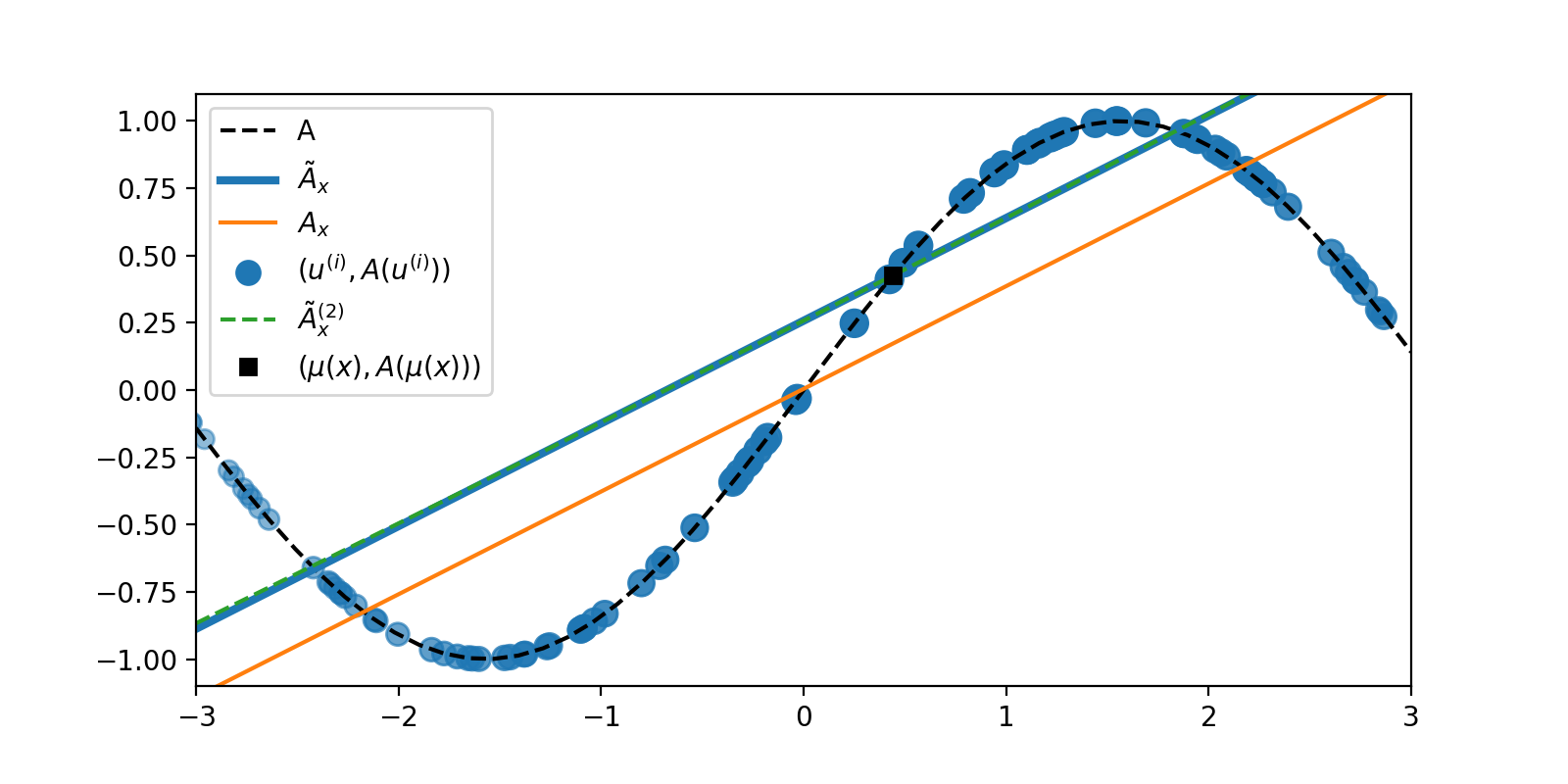
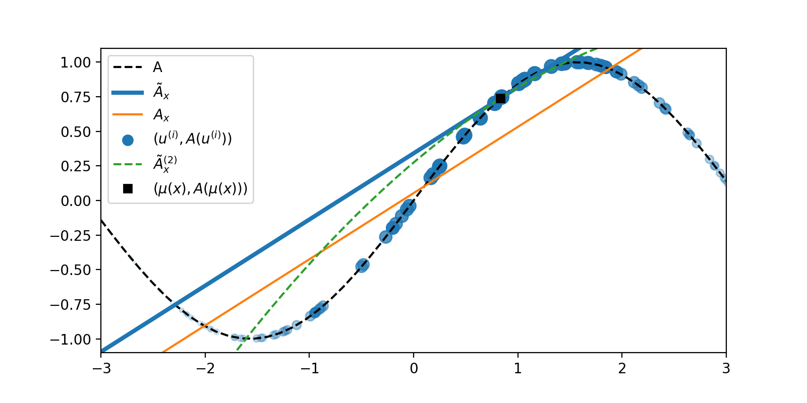
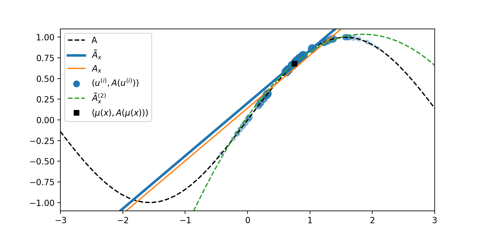
Figure 1: Local frame-based approximation with (Gaussian) kernel bandwidths $r\in\{5,1,0.2\}$ (top to bottom) for the sine function, with an ensemble of size $J=100$ uniformly sampled on the interval $[-3,3]$.

Himmelblau function.

Here, we consider $\mathcal{X}=\mathbb{R}^{2}$ and $\mathcal{Y}=\mathbb{R}$, with $A(x)$ being the Himmelblau function. We generate an ensemble with $J=100$ particles according to a Gaussian distribution and pick one arbitrary ensemble member $u^{(i)}$ as a reference point $x$. Figures 2 and 3 show the resulting approximations $A_{x}$ and $A_{x}^{(2)}$ in reference to the original function, and to its exact second-order Taylor approximation at $x$.

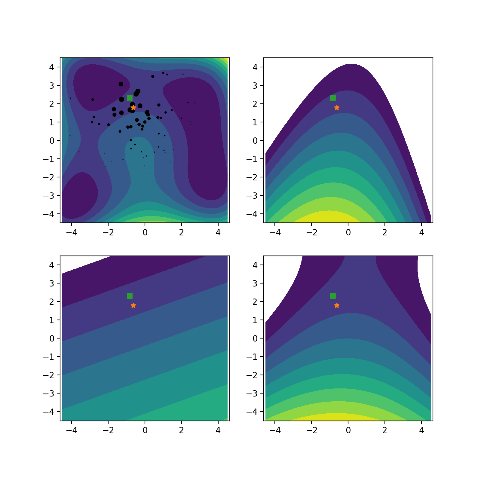
Figure 2: Local frame-based approximation with (Gaussian) kernel bandwidth $r=1$. Ensemble size $J=100$. Top left: Contour plot of the Himmelblau function. Green square marker: Reference point $x$. Black markers: Ensemble members (with marker size proportional to weight $\kappa^{(i)}(x)$). Orange star: locally weighted ensemble mean $\mu^{\kappa}(x)$. Top right: Contour plot of (exact) second-order Taylor approximation centered at $\mu^{\kappa}(x)$. Bottom left: Approximate first order approximation $A_{x}$. Bottom right: Approximate second-order approximation $A_{x}^{(2)}$.

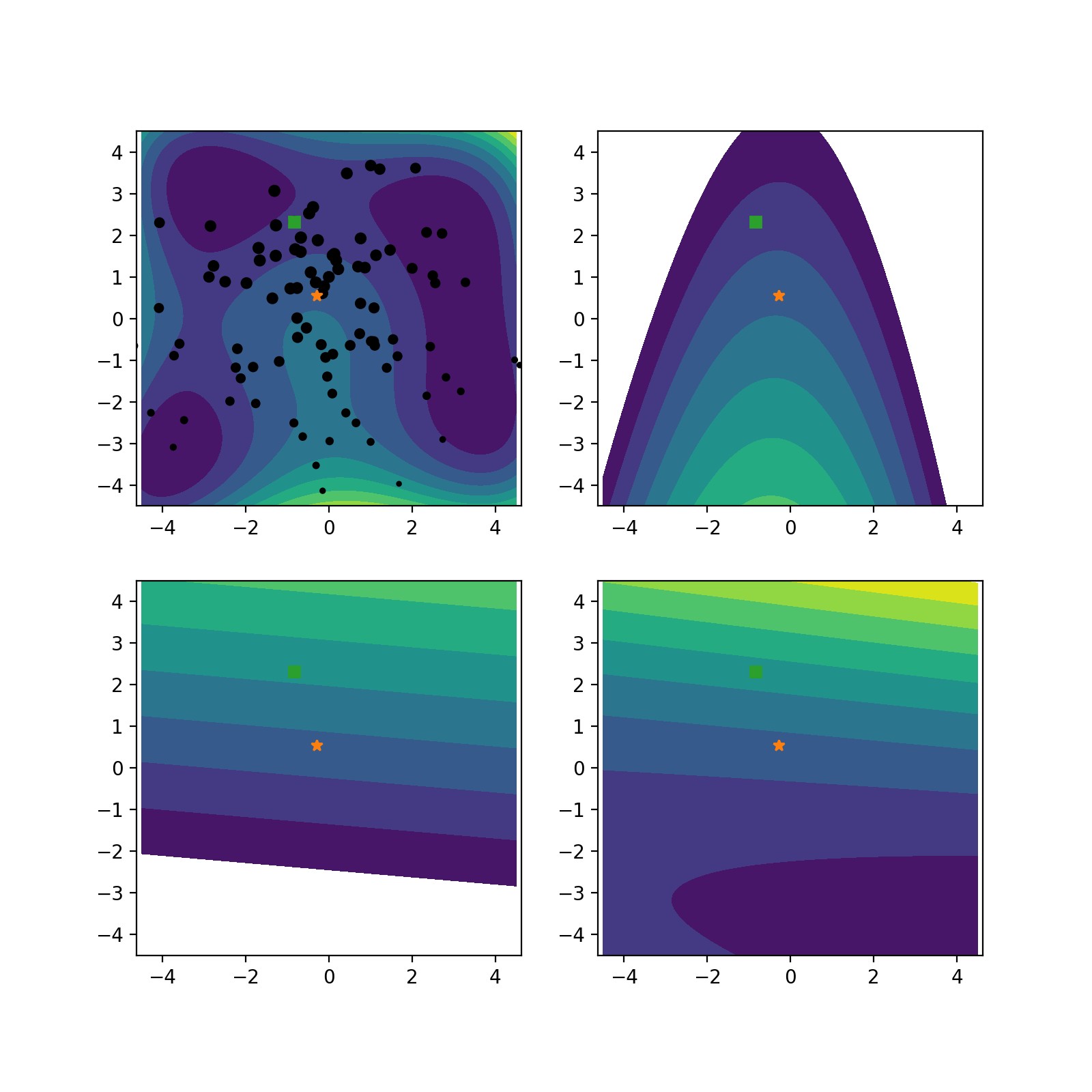
Figure 3: Local frame-based approximation with (Gaussian) kernel bandwidth $r=5$. Ensemble size $J=100$. Top left: Contour plot of the Himmelblau function. Green square marker: Reference point $x$. Black markers: Ensemble members (with marker size proportional to weight $\kappa^{(i)}(x)$), identical ensemble as in figure 2. Orange star: locally weighted ensemble mean $\mu^{\kappa}(x)$. Top right: Contour plot of (exact) second-order Taylor approximation centered at $\mu^{\kappa}(x)$. Note that this is different from the top right plot in figure 2 because $\mu^{\kappa}(x)$ depends on the kernel and its bandwidth. Bottom left: Approximate first order approximation $A_{x}$. Bottom right: Approximate second-order approximation $A_{x}^{(2)}$.

4 Locally weighted ensemble Kalman-type methods

Now that we have set up a solid concept of locally weighted linear approximation, it is very straightforward to define a locally weighted EK method by replacing the empirical covariance in the definition of the linear EK by its weighted variant:

Definition 4.

With the definition of locally weighted covariance above, we define the locally weighted EK method as the system of ODEs given by

$$\frac{\mathrm{d}}{\mathrm{d}t}u^{(i)} =-C_{u,A}^{\kappa}(u^{(i)})\cdot\left(A(u^{(i)})-y\right)$$

This means that locally weighted EK just replaces moments like $\mu$, $C_{u,A}$, etc., by their $\kappa$-weighted variants. In a similar way we can modify other algorithms based on the Ensemble Kalman method, such as the EnKF, ALDI, etc.

The hard work in analysing $D_{\kappa}$ pays off now because the following lemma is trivially true by definition of $D_{\kappa}$.

Lemma 6.

The locally weighted EK method can equivalently be defined as

$$\frac{\mathrm{d}}{\mathrm{d}t}u^{(i)} =-C_{u,u}^{\kappa}(u^{(i)})(D_{\kappa}A(u^{(i)}))^{\top}(A(u^{(i)})-y)$$

$$=-\sum_{j=1}^{J}\kappa^{(j)}(u^{(i)})(u^{(j)}-\mu(u^{(i)}))\left\langle A(u^{(j)})-\mu_{A}(u^{(i)}),A(u^{(i)})-y\right\rangle$$

Note the similarity of this relation to (6).

Remark 3.

Locally weighted EKI is in general not equivalent to the system of ODEs given by

$$\frac{\mathrm{d}}{\mathrm{d}t}u^{(i)} =-C_{u,u}^{\kappa}(u^{(i)})D_{\kappa}\Phi(u^{(i)}).$$

4.1 Numerical experiments

We consider a numerical experiment based on the “Himmelblau” optimisation benchmark function. Let

$$A(x_{1},x_{2})=(x_{1}^{2}+x_{2},x_{1}+x_{2}^{2})$$ (37)

and consider a data/target value $y=(11,7)^{\top}$. We can define a cost/misfit functional $\Phi(u)=\frac{1}{2}\|y-A(u)\|^{2}$. Minimisers of this potential are the four solutions to $A(x)=y$ and can be observed as being the minima of the misfit functional $\Phi$ (which happens to be the Himmelblau function), as shown in figure 4. We generate an ensemble with $J=100$ particles and perform locally weighted EK with a Gaussian kernel with bandwidth $1$. The results are shown in figure 4 and it can be observed that the locally weighted EK method successfully finds all four global minima.

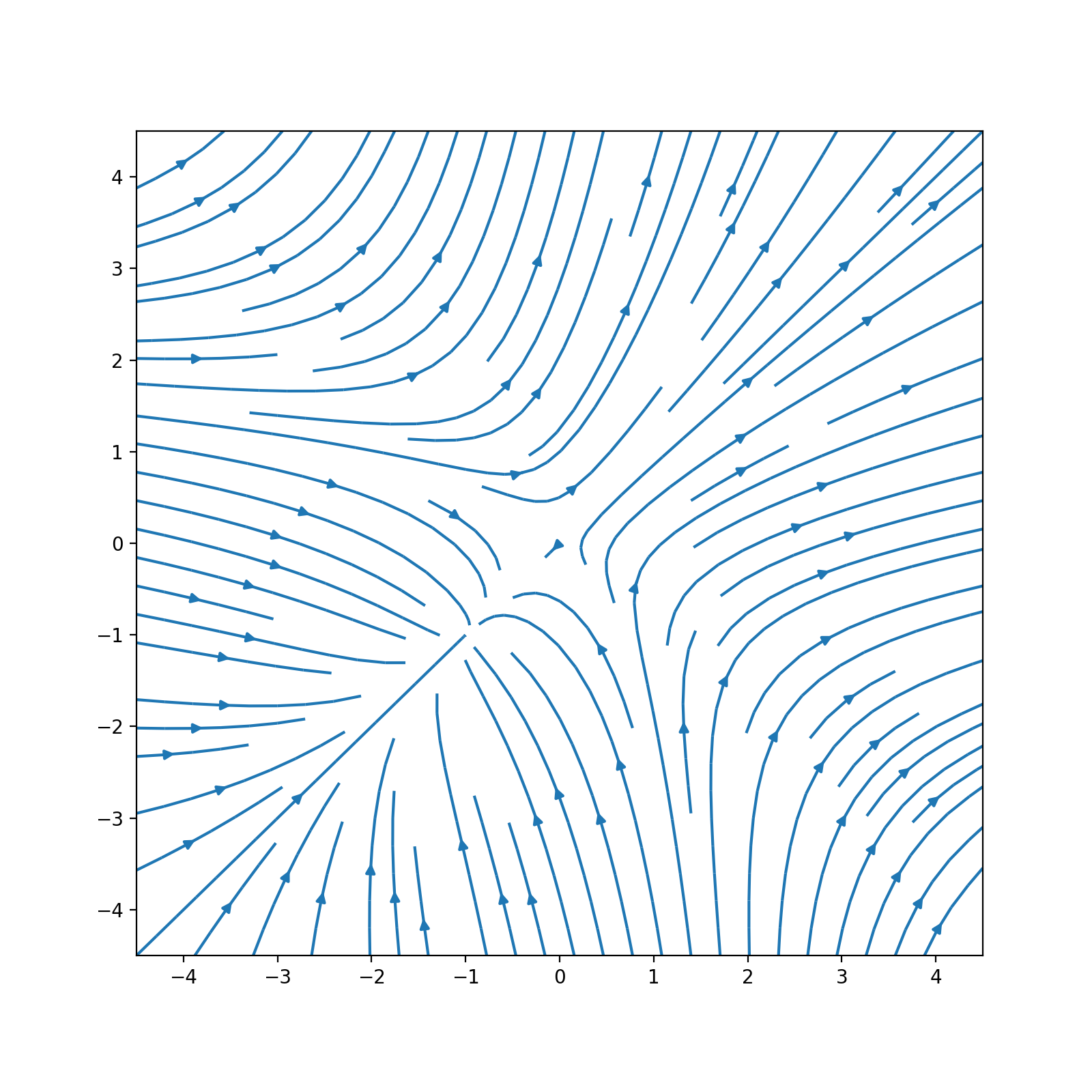
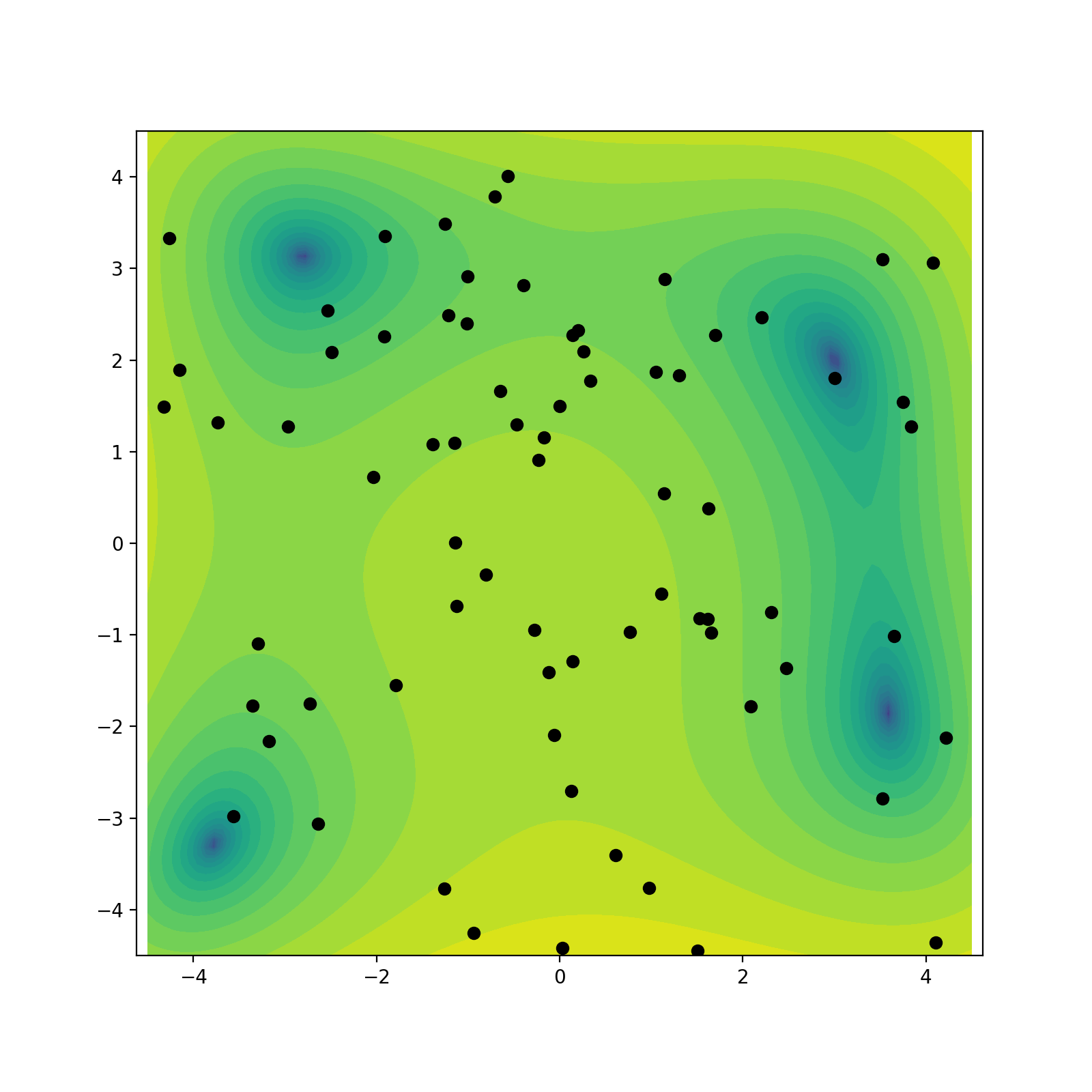
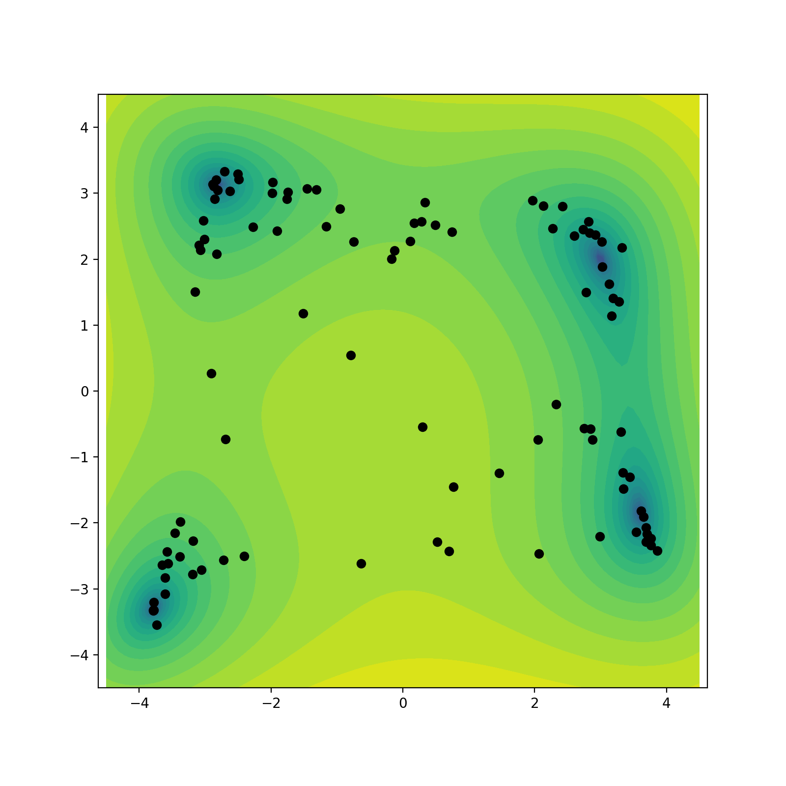
Figure 4: Map $A:\mathbb{R}^{2}\to\mathbb{R}^{2}$ (top left, visualised as a vector field) and resulting misfit functional $\Phi$ (top right, with initial ensemble). Inversion of $Au=y$ amounts to minimisation of $\Phi$. Bottom row: Evolution of initial ensemble through locally weighted EK with a Gaussian kernel of bandwidth $1$. Ensemble eventually collapses to all four global minima (not shown).

We compare this with the linear EK in figure 5. It can be observed that the ensemble collapses on one of the four global minima. This should be considered a best-case scenario because it is entirely possible that the linear EK method stops prematurely due to its empirical covariance becoming singular, as discussed above.

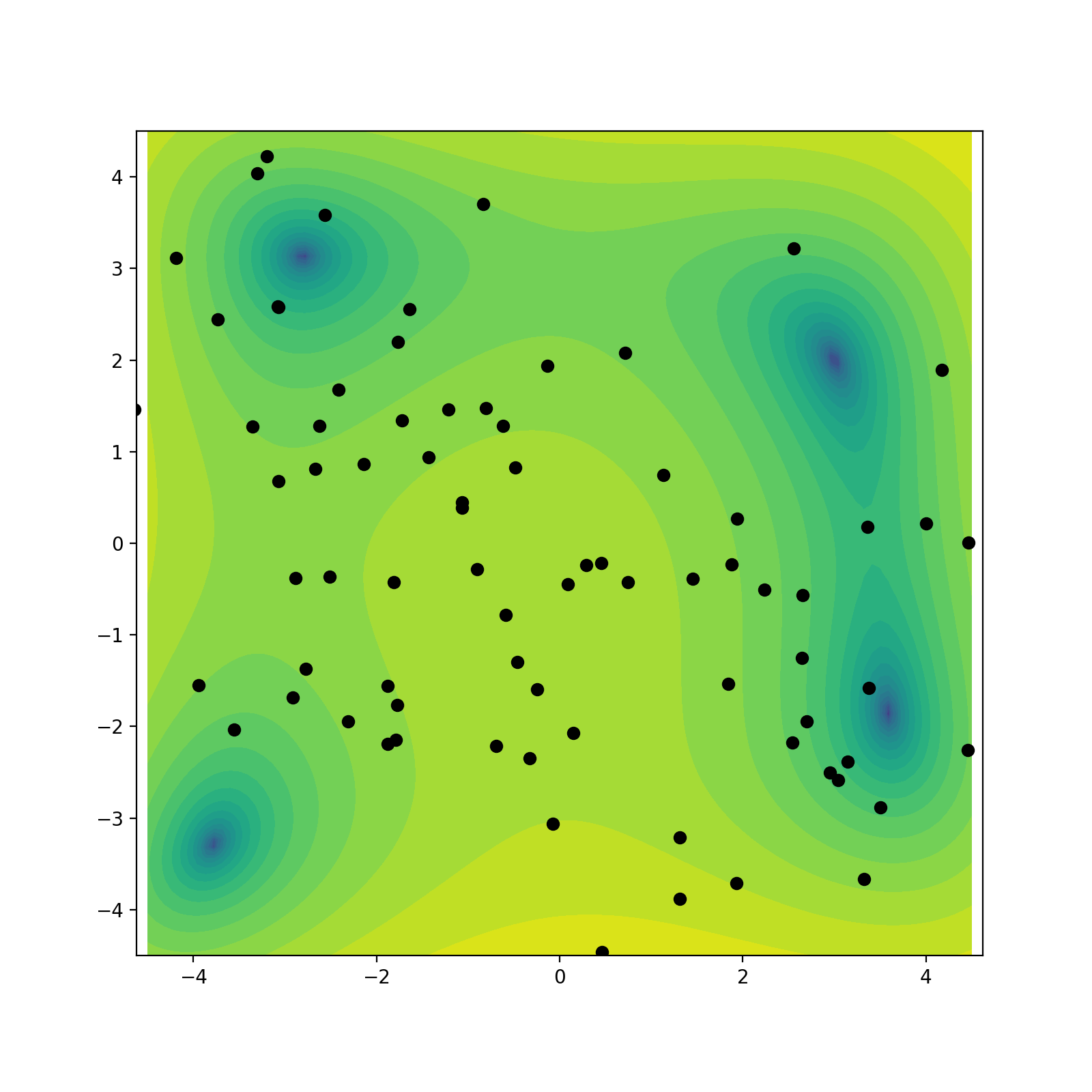
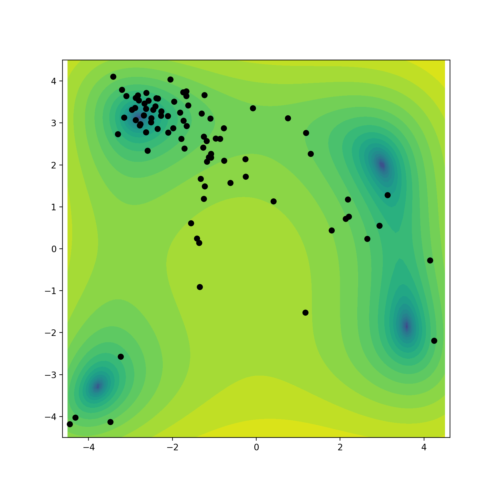
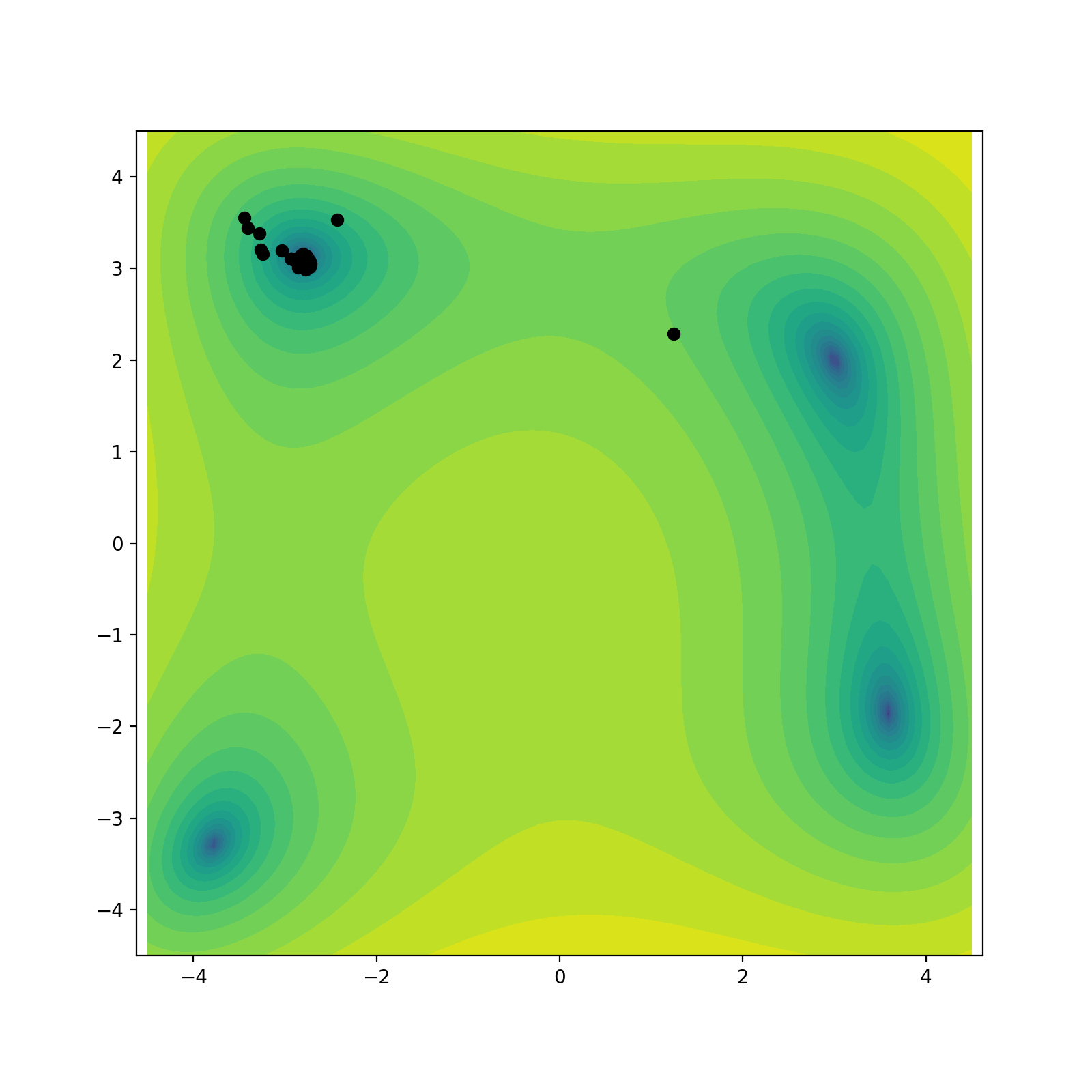
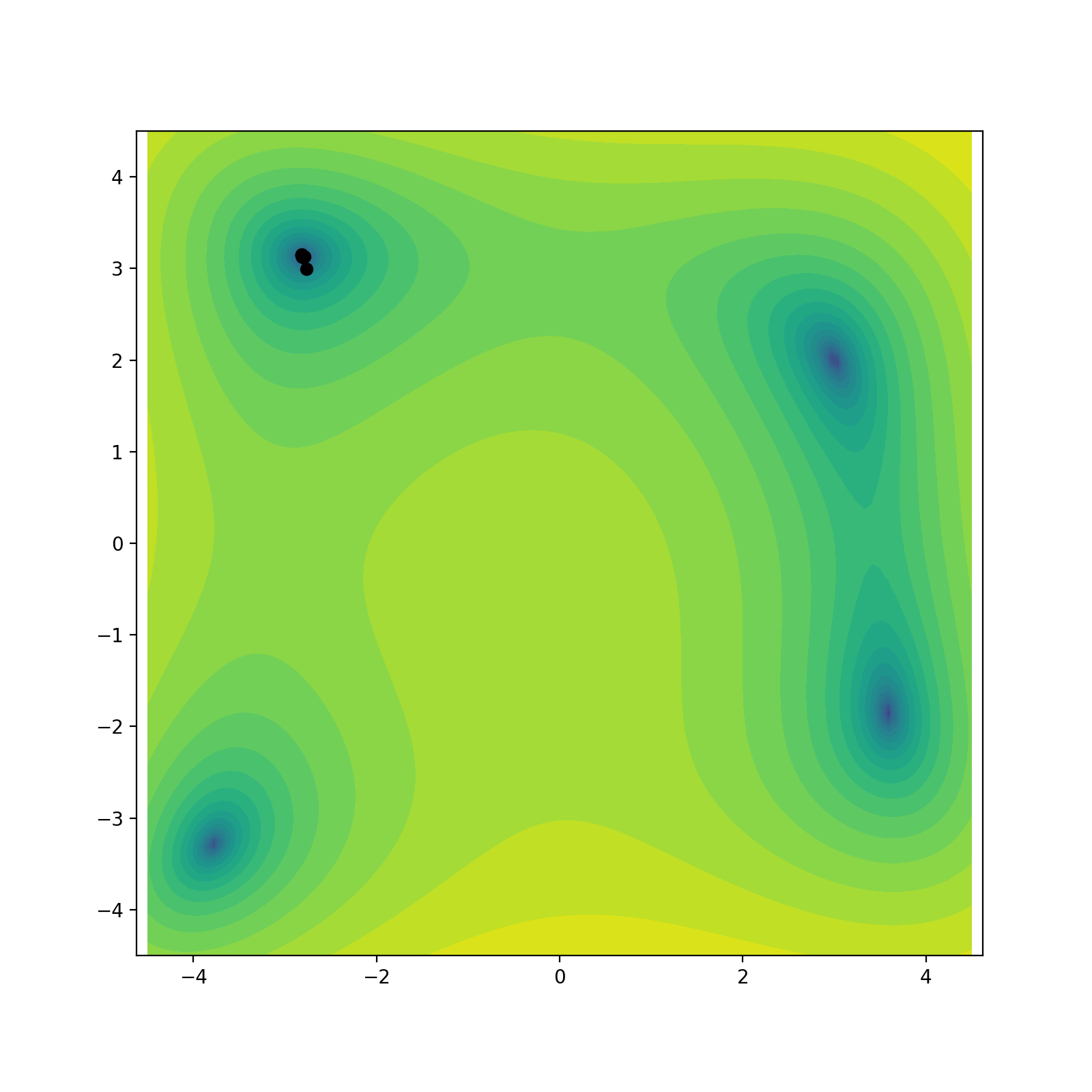
Figure 5: Evolution of initial ensemble through linear EK. Ensemble eventually collapses to only one of the four global minima.

4.2 Challenges and outlook

The elephant in the room regarding the locally weighted EK is the larger computational overhead (as compared to the linear EK): Since moments have to be generated for each particle, rather than just for the whole ensemble, this creates considerable computational cost for large ensemble sizes. There are several ways of mitigating this issue: For a sufficiently quickly decaying kernel, the locally weighted covariances have a very low-rank structure, which can possibly be used for computational speed-up. Alternatively, we can further modify the locally weighted EK method using ideas of the “cluster-based” variant of polarCBO in [BRW22]: By fixing a number of clusters $M$, and relating all particles to clusters instead of all particles with each other, we only need $\mathcal{O}(M\cdot J)$ comparisons, rather than $\mathcal{O}(J^{2})$. This idea was already proposed by [WPU22] in the context of rare event estimation. Thirdly, we can use the kernel to build a graph structure on the ensemble, where there is an edge between particles $u^{(i)},u^{(j)}$ if the weight $k(u^{(i)},u^{(j)})$ is positive (or larger than some threshold). Then graph-based message-passing algorithms can be utilised to improve efficiency of computation.

But not only large value of ensemble size $J$ are problematic: If the dimensionality of parameter space is very high, radial distance-based local weighting will have performance issues due to the curse of dimensionality: Since relative volumes of balls of fixed radius have asymptotically vanishing values, it becomes harder and harder to find ensemble members which are not getting weighted down to $0$ by the kernel function. This can be remedied by, e.g., utilising lower-dimensional structure or replacing distance-based local weights by something more robust.

A more realistic feasibility test of the locally weighted Ensemble Kalman method would be a test of performance in a filter setting. It would be interesting to see whether the locally weighted EnKF is able to combine the speed of the EnKF with the flexibility of a particle filter in a nonlinear filtering setup.

Another interesting question is whether the kernel bandwidth should be kept fixed throughout, adapted, or even locally adapted (for example based on the locally weighted covariance, closing this loop, too). We refer further elaboration of these considerations to future research.

References

- [BK98] David Matthew Bortz and Carl Tim Kelley “The simplex gradient and noisy optimization problems” In Computational Methods for Optimal Design and Control: Proceedings of the AFOSR Workshop on Optimal Design and Control Arlington, Virginia 30 September–3 October, 1997, 1998, pp. 77–90 Springer
- [Blö+19] Dirk Blömker, Claudia Schillings, Philipp Wacker and Simon Weissmann “Well posedness and convergence analysis of the ensemble Kalman inversion” In Inverse Problems 35.8 IOP Publishing, 2019, pp. 085007
- [BRW22] Leon Bungert, Tim Roith and Philipp Wacker “Polarized consensus-based dynamics for optimization and sampling” In arXiv preprint arXiv:2211.05238, 2022
- [CDV08] AL Custódio, JE Dennis and Luıs Nunes Vicente “Using simplex gradients of nonsmooth functions in direct search methods” In IMA journal of numerical analysis 28.4 OUP, 2008, pp. 770–784
- [CKP13] Peter G Casazza, Gitta Kutyniok and Friedrich Philipp “Introduction to finite frame theory” In Finite frames: theory and applications Springer, 2013, pp. 1–53
- [Cle79] William S Cleveland “Robust locally weighted regression and smoothing scatterplots” In Journal of the American statistical association 74.368 Taylor & Francis, 1979, pp. 829–836
- [CRS22] Edoardo Calvello, Sebastian Reich and Andrew M Stuart “Ensemble Kalman methods: A mean field perspective” In arXiv preprint arXiv:2209.11371, 2022
- [CST20] Neil K Chada, Andrew M Stuart and Xin T Tong “Tikhonov regularization within ensemble Kalman inversion” In SIAM Journal on Numerical Analysis 58.2 SIAM, 2020, pp. 1263–1294
- [CSV09] Andrew R Conn, Katya Scheinberg and Luis N Vicente “Introduction to derivative-free optimization” SIAM, 2009
- [CT19] Ian Coope and Rachael Tappenden “Efficient calculation of regular simplex gradients” In Computational Optimization and Applications 72 Springer, 2019, pp. 561–588
- [ESS15] Oliver G Ernst, Björn Sprungk and Hans-Jörg Starkloff “Analysis of the ensemble and polynomial chaos Kalman filters in Bayesian inverse problems” In SIAM/ASA Journal on Uncertainty Quantification 3.1 SIAM, 2015, pp. 823–851
- [Eve03] Geir Evensen “The ensemble Kalman filter: Theoretical formulation and practical implementation” In Ocean dynamics 53 Springer, 2003, pp. 343–367
- [FK13] Marco Frei and Hans R Künsch “Bridging the ensemble Kalman and particle filters” In Biometrika 100.4 Oxford University Press, 2013, pp. 781–800
- [Gar+20] Alfredo Garbuno-Inigo, Franca Hoffmann, Wuchen Li and Andrew M Stuart “Interacting Langevin diffusions: Gradient structure and ensemble Kalman sampler” In SIAM Journal on Applied Dynamical Systems 19.1 SIAM, 2020, pp. 412–441
- [GNR20] Alfredo Garbuno-Inigo, Nikolas Nüsken and Sebastian Reich “Affine invariant interacting Langevin dynamics for Bayesian inference” In SIAM Journal on Applied Dynamical Systems 19.3 SIAM, 2020, pp. 1633–1658
- [ILS13] Marco A Iglesias, Kody JH Law and Andrew M Stuart “Ensemble Kalman methods for inverse problems” In Inverse Problems 29.4 IOP Publishing, 2013, pp. 045001
- [Kal60] Rudolph Emil Kalman “A New Approach to Linear Filtering and Prediction Problems” In Transactions of the ASME–Journal of Basic Engineering 82.Series D, 1960, pp. 35–45
- [PP+08] Kaare Brandt Petersen and Michael Syskind Pedersen “The matrix cookbook” In Technical University of Denmark 7.15, 2008, pp. 510
- [RW21] Sebastian Reich and Simon Weissmann “Fokker–Planck particle systems for Bayesian inference: Computational approaches” In SIAM/ASA Journal on Uncertainty Quantification 9.2 SIAM, 2021, pp. 446–482
- [SS17] Claudia Schillings and Andrew M Stuart “Analysis of the ensemble Kalman filter for inverse problems” In SIAM Journal on Numerical Analysis 55.3 SIAM, 2017, pp. 1264–1290
- [SSW20] Claudia Schillings, Björn Sprungk and Philipp Wacker “On the convergence of the Laplace approximation and noise-level-robustness of Laplace-based Monte Carlo methods for Bayesian inverse problems” In Numerische Mathematik 145 Springer, 2020, pp. 915–971
- [Sto+11] Andreas S Stordal et al. “Bridging the ensemble Kalman filter and particle filters: the adaptive Gaussian mixture filter” In Computational Geosciences 15 Springer, 2011, pp. 293–305
- [STW23] Claudia Schillings, Claudia Totzeck and Philipp Wacker “Ensemble-based gradient inference for particle methods in optimization and sampling” In SIAM/ASA Journal on Uncertainty Quantification 11.3 SIAM, 2023, pp. 757–787
- [Tip+03] Michael K Tippett et al. “Ensemble square root filters” In Monthly weather review 131.7 American Meteorological Society, 2003, pp. 1485–1490
- [Van+19] Peter Jan Van Leeuwen et al. “Particle filters for high-dimensional geoscience applications: A review” In Quarterly Journal of the Royal Meteorological Society 145.723 Wiley Online Library, 2019, pp. 2335–2365
- [Won01] Roderick Wong “Asymptotic approximations of integrals” SIAM, 2001
- [WPU22] Fabian Wagner, Iason Papaioannou and Elisabeth Ullmann “The ensemble Kalman filter for rare event estimation” In SIAM/ASA Journal on Uncertainty Quantification 10.1 SIAM, 2022, pp. 317–349