Markovian embedding of nonlocal equations using spectral representation

Abstract

Nonlocal evolutionary equations containing memory terms model a variety of non-Markovian processes. We present a Markovian embedding procedure for a class of nonlocal equations by utilising the spectral representation of the nonlinear memory kernel. This allows us to transform the nonlocal system to a local-in-time system in an abstract extended space. We demonstrate our embedding procedure and its efficacy for two different physical models, namely the $(i)$ $1$D walking droplet and the $(ii)$ $1$D single-phase Stefan problem.

[inst1]organization=International Centre for Theoretical Sciences, Tata Institute of Fundamental Research, city=Bengaluru, postcode=560089, country=India [inst2]organization=School of Computer and Mathematical Sciences, University of Adelaide, postcode=5005, country=Australia

1 Introduction

Several evolutionary processes with memory effects are modelled by nonlocal equations. Examples include particle motion in unsteady hydrodynamic environments (Lovalenti and Brady, 1993; Oza et al., 2013; Peng and Schnitzer, 2023), and boundary evolution in diffusion processes in time-dependent domains (Stefan, 1891; Fokas and Pelloni, 2012) and under nonlinear boundary forcing (Mann and Wolf, 1951; Keller and Olmstead, 1972; Olmstead and Handelsman, 1976). In this manuscript, we are concerned with nonlocal models where the evolution equation for a state variable $y(t)$ has the following canonical structure:

$${}y^{(n)}(t)=L(t,y(t))+\int_{0}^{t}N(y(t),y(s),t-s)\>ds~{},$$ (1)

where the superscript $n$ indicates the order of time derivative. The function $L(\cdot)$ is a local-in-time term driving the evolution, whereas the function $N(\cdot)$ is a memory kernel of the nonlocal integral, which is also a nonlinear function of $y(t)$. Without the nonlocal term, Eq. (1) can be readily transformed into a system of first order ordinary differential equations (ODEs) yielding a Markovian description. However, with the nonlocal term, such a transformation is not trivial. Different Markovian embeddings in an abstract extended space are commonly realised by introducing an auxiliary variable that accounts for the memory (Dafermos, 1970). In this study, we show that a Markovian prescription can be realised for nonlocal equations of the form in Eq. (1) by an embedding procedure that relies on the spectral representation of the nonlinear memory kernel (previously discussed for linear memory kernel in (Jaganathan et al., 2023)).

Our approach involves expressing the nonlocal integral term in Eq. (1) as a local-in-time term. We assume that the nonlinear memory kernel has a spectral representation of the following form:

$${}N(y(t),y(s),t-s)=\int_{\Gamma}e^{\phi(k;y(t),y(s),t-s)}\psi(k,y(s))\>dk~{},$$ (2)

where $\Gamma$ is a smooth contour in the complex-plane and $\phi,\psi$ are complex-analytic functions of the variable $k$. The spectral representation allows embedding of Eq. (1) into an extended space. This is done by substituting the spectral representation in the memory term, followed by an interchange of order of integrals, to give:

$$\int_{0}^{t}\int_{\Gamma}e^{\phi(k;y(t),y(s),t-s)}\psi(k,y(s))\>dk\>ds=:\int_{\Gamma}H(k,t)\>dk$$

where $H(k,t)$ is the newly-introduced complex-valued auxiliary variable. Since it encapsulates “memory”, we refer to it as the history function. Owing to the particular spectral form, we can infer that the history function has a Markovian evolution given by an ODE, parameterised by the spectral variable $k$. Therefore, we have the following local-in-time reformulation of Eq. (1) in an infinite-dimensional space:

$$y^{(n)}(t) =L(t,y(t))+\int_{\Gamma}H(k,t)\>dk~{},$$ (3a)

$$\dot{H}(k,t) =\dot{\phi}(k;y(t))H(k,t)+e^{\phi(k;y(t))}\psi(k,y(t))~{},$$ (3b)

where overdot denotes time derivative.

2 Prototypical physical models with nonlinear memory effects

We demonstrate our embedding procedure for two physical models with nonlinear memory effects, namely the one-dimensional walking droplet and the single-phase one-dimensional Stefan problem. Both models illustrate that a Markovian embedding into an infinite-dimensional space can be constructed subject to a natural spectral representation of the nonlinear memory kernel (Eq. (2)). These models differ in the complexity of the auxiliary history variable introduced upon embedding, highlighting the versatility of the approach.

2.1 Walking droplets

A hydrodynamic active system described by non-Markovian dynamics is that of walking (Couder et al., 2005) and superwalking (Valani et al., 2019) droplets. By vertically vibrating an oil bath, a drop of the same oil can be made to bounce and walk on the liquid surface. Each bounce of the droplet locally excites a damped standing wave. The droplet interacts obliquely with these self-excited waves on subsequent bounces to propel itself horizontally, giving rise to a self-propelled, classical wave-particle entity (WPE). At large vibration amplitudes, the droplet-generated waves decay slowly in time. Hence, the motion of the droplet is affected by the history of waves along its trajectory. This gives rise to path memory in the system and makes the dynamics non-Markovian.

Oza et al. (Oza et al., 2013) developed a theoretical stroboscopic model to describe the horizontal walking motion of such a WPE. The model averages over the fast vertical periodic bouncing of the droplet and provides a trajectory equation for the slow walking dynamics in the horizontal plane. We consider a reduction of this model to one horizontal dimension, $x\in\mathbb{R}$ (see Fig. 1a). Consider a droplet with position and velocity given by $(x_{d}(t),\dot{x}_{d}(t))\in\mathbb{R}^{2}$, which continuously generates standing waves with prescribed spatial structure $W(x)$ that decay with time. The dynamics of a $1$D WPE follows the non-dimensional integro-differential equation:

$${}\ddot{x}_{d}(t)=-\dot{x}_{d}(t)-C_{1}\int_{0}^{t}W^{\prime}(x_{d}(t)-x_{d}(s))K(t-s;C_{2})\>ds,$$ (4)

where $C_{1}$ and $C_{2}$ are non-negative constants representing dimensionless wave-amplitude and inverse memory parameter, respectively. We refer the reader to Ref. (Oza et al., 2013) for details and explicit expressions for these parameters. Eq. (4) is a horizontal force balance of the WPE with the right-hand side containing an effective drag term proportional to velocity $-\dot{x}_{d}(t)$ and the nonlocal memory term capturing the cumulative force on the particle from the superposition of the self-generated waves along its path. The memory kernel comprises the functions $W^{\prime}(\cdot)$ and $K(\cdot)$; the former represents the wave-gradient where the prime denotes derivative with respect to its argument, and $K(\cdot)$ imposes the temporal decay. In the stroboscopic model of a walking droplet, $-W^{\prime}(x)=J_{1}(x)$, where $J_{1}$ is the Bessel-$J$ function of order one and $K(t)=e^{-C_{2}t}$.

In the high-memory regime ($C_{2}\ll 1$), WPEs exhibit hydrodynamic quantum analogs (Bush and Oza, 2020). However, the regime may become experimentally difficult to access (Bacot et al., 2019) due to the increased susceptibility of the system to the Faraday instability (Faraday, 1831). Numerical simulations provide an alternative with controllability but also entail dealing with the non-Markovian structure of Eq. (4) and time-dependent computational costs therein.

2.1.1 Markovian embedding for the stroboscopic model

We convert Eq.(4) to a Markovian description in the following way. We recall the following integral representation of the Bessel-$J_{1}$ function for some $z\in\mathbb{R}$:

$$J_{1}(z)=-\frac{i}{\pi}\int_{-1}^{1}e^{ikz}\frac{k}{\sqrt{1-k^{2}}}\>dk~{}.$$

Substituting the above in the memory term of Eq. (4), followed by a switch in the order of integrals, we construct the equivalent local-in-time representation for the memory integral,

$$-\frac{i}{\pi}\int_{0}^{t}\int_{-1}^{1}e^{ik(x_{d}(t)-x_{d}(s))-C_{2}(t-s)}\frac{k}{\sqrt{1-k^{2}}}\>dk\>ds=:\int_{-1}^{1}H(k,t)w(k)\>dk$$

where the weight function $w(k)=1/\sqrt{1-k^{2}}$ and $H(k,t)$ is a complex-valued function of time $t$ and a real number $k$ with a finite support in $[-1,1]$. The induced definition of $H(k,t)$ is

$${}H(k,t):=-\frac{ik}{\pi}\int_{0}^{t}e^{ik(x_{d}(t)-x_{d}(s))-C_{2}(t-s)}\>ds~{}.$$ (5)

The form of $H(\cdot)$ in (5) suggests that it has a Markovian evolution according to an ODE parameterised by the spectral variable $k$. Consequently, combined with the definition of the droplet’s velocity $\dot{x}_{d}=v_{d}$, we derive the following Markovian prescription for the WPE dynamics in the extended state space for $t>0$:

$$\dot{v}_{d}(t) =-v_{d}(t)+C_{1}\int_{-1}^{1}H(k,t)w(k)\>dk,$$ (6a)

$$\dot{H}(k,t) =-C_{2}H(k,t)+ikv_{d}(t)H(k,t)-\frac{ik}{\pi}~{},$$ (6b)

subject to initial conditions $(x_{d0},v_{d0})$ and $H(k,0)=0$. We note in Eq. (5) that $H(\cdot)$ preserves certain symmetries with respect to the spectral variable $k$ at all times: $\text{Re}(H)$ has an even-symmetry whereas $\text{Im}(H)$ is odd-symmetric. Therefore, whereas the real and imaginary parts of the history function drive each other’s dynamics, only the real part contributes to the memory integral in Eq. (6a).

The resultant set of local differential equations (6) can be readily solved using any standard time-integrator; we use the second-order Runge-Kutta scheme. An additional task involves computing the history integral over $k$. The integrand, with its finite support in $[-1,1]$ and the form of weight function $w$, naturally suggests expansion of $H(k,t)$ in the bases of Chebyshev polynomials of the first kind. Therefore, we use the spectrally-accurate Clenshaw-Curtis quadrature method to approximate the integral:

$$\int_{-1}^{1}H(k,t)w(k)\>dk\approx\sum_{n=0}^{M}\omega_{n}H(k_{n},t),\quad M\in\mathbb{N}~{},$$

where $k_{n}=\cos(n\pi/M)$ are the Chebyshev nodes and $\omega_{n}$ are the associated weights. We numerically solve Eq. (6) for a few representative parameter sets $(C_{1},C_{2})$. Fig. 1 shows that the embedded system of equations (6) successfully reproduces the previously known non-walking and walking regimes in the parameter space (Durey et al., 2020; Valani et al., 2021). For a steady walker, an analytical expression for its steady speed (Oza et al., 2013) is :

$${}v_{d}^{\infty}=\frac{1}{\sqrt{2}}\sqrt{2C_{1}-C_{2}^{2}-\sqrt{C_{2}^{4}+4C_{1}C_{2}^{2}}}~{}.$$ (7)

The numerical solution for the steady walker attains the above analytical steady walking speed (dashed line) in Fig. 1c. Additionally, in Fig. 2, we show the evolution of the history function in the $k-$domain over time.

There have been previous works (Moláček, 2013; Durey et al., 2020; Durey, 2020; Valani, 2022) that rewrite the integro-differential equation for the walker into a system of ODEs. However, these transformations work for only specific choices of the wave form $W(x)$. The Markovian embedding formalism is applicable for a broader class of wave forms that have a suitable spectral representation. This is particularly useful in generalised pilot-wave framework, where new hydrodynamic quantum analogues are being explored by investigating various wave forms (Bush and Oza, 2020).

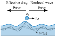
(a)

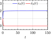
(b)

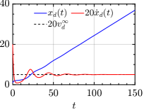
(c)

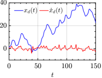
(d)

​ ​

Figure 1: (a) Schematic of a 1D walking droplet. Typical known droplet states in the stroboscopic model obtained by solving the Markovian system (Eq. (6)) for $(x_{d0},\dot{x}_{d0})$ = $(1,1)$: (b) Non-walker $(C_{1}=0.01,C_{2}=0.1)$, (c) Steady walker $(C_{1}=C_{2}=0.1)$, (d) Chaotic walker $(C_{1}=1.5,C_{2}=0.01)$. Velocity in (c) is scaled by a factor of $20$ for visibility.

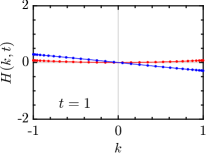
(a)

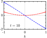
(b)

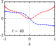
(c)

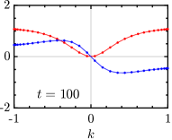
(d)

​ ​ ​

Figure 2: Evolution of real (red)/imaginary (blue) parts of the history function $H(k,t)$ at representative times for a steady walker $(C_{1}=C_{2}=0.1)$, with $H(k,0)=0$. The finite support of $H(k,t)$ in $[-1,1]$ and its smoothness demands a nominal, fixed (in time) requirement of as few as $M=30$ Chebyshev quadrature nodes to accurately compute the history integral.

2.2 Single-phase Stefan problem

We now consider the class of free boundary problems called the Stefan problem, which primarily describes phase-change processes such as the melting of a solid (Stefan, 1891; Guenther and Lee, 2012). In its simplest non-dimensional formulation, it comprises a one-dimensional domain in $\mathbb{R}^{+}$, contiguously supporting a molten phase and a solid phase, separated at their interface, which is free to move as the solid melts (see Fig. 3a). The solid phase is modelled as an infinite heat sink maintained at the melting temperature at all times. Therefore, the simplified problem involves finding the solution pair $(\theta(x,t),l(t))$, where $\theta(x,t)$ describes the instantaneous temperature distribution in the molten phase and $l(t)$ is the location of the melting front. The function $\theta$ satisfies the diffusion equation $\partial_{t}\theta-\partial_{x}^{2}\theta=0$ in $x\in[0,l(t)]$, subject to an arbitrary initial condition $\theta_{0}(x)$ in the initial domain $x\in[0,l_{0}]$ at $t=t_{0}$, and a temperature or heat flux condition at the fixed boundary $x=0$. The moving front, which is at the melting temperature, is governed by the Stefan condition $\dot{l}=-\partial_{x}\theta(l(t),t)$.

We consider the case where temperature is prescribed at the fixed boundary, $\theta(0,t)=f(t)$ for exposition. With primary interest in the interface’s location, the bulk heat diffusion process in the molten phase may be effectively “integrated out” to derive a non-Markovian equation of motion for the moving front. The resulting velocity equation for the moving front, $v(t)=\dot{l}(t)$, is compactly written in the following nonlinear Volterra integral form for $t>t_{0}$ (Fokas and Pelloni, 2012; Guenther and Lee, 2012):

$$v(t)=g(t-t_{0},l(t);\theta_{0}^{\prime},l_{0})+\int_{t_{0}}^{t}N(l(t),l(s),t-s;v(s),\dot{f}(s))\>ds$$ (8)

where $\theta_{0}^{\prime},\dot{f}$ denote the spatial derivative and temporal derivative of $\theta_{0},f$ respectively, and the function $g$ is:

$$g(t-t_{0},l(t);\theta_{0}^{\prime},l_{0})=-\frac{1}{\sqrt{\pi(t-t_{0})}}\int_{0}^{l_{0}}\Big{(}e^{-(l(t)+x)^{2}/4(t-t_{0})}+e^{-(l(t)-x)^{2}/4(t-t_{0})}\Big{)}\theta_{0}^{\prime}(x)\>dx~{}.$$ (9)

The nonlinear kernel may be decomposed into contributions from forcing at the fixed boundary and the unknown velocity of the solid-liquid interface as follows:

$${}N(l(t),l(s),t-s;v(s),\dot{f}(s))=v(s)N_{1}(l(t),l(s),t-s)+\dot{f}(s)N_{2}(l(t),0,t-s)~{},$$ (10)

with the definitions

$$N_{1}(x,y,z)=\frac{1}{2\sqrt{\pi}}\Bigg{(}\frac{(x+y)e^{-(x+y)^{2}/4z}-(x-y)e^{-(x-y)^{2}/4z}}{z^{3/2}}\Bigg{)},\quad N_{2}(x,y,z)=\frac{2}{\sqrt{\pi}}\frac{e^{-x^{2}/4z}}{z^{1/2}}~{}.$$

Note that the function $g$ is a local-in-time term. The second term on the right-hand side in Eq. (8) is the memory term, which introduces non-locality and the nonlinear dependence on the moving front $l(t)$.

2.2.1 Markovian embedding for Stefan problem

As before, we construct an embedding such that the present non-Markovian representation for $v(t)$ may be turned Markovian. We claim the following spectral representation of the nonlinear kernel for a real $k$:

$$N_{1}(x,y,z) =\int_{-\infty}^{\infty}dN_{1}(k;x,y,z)=\frac{i}{\pi}\int_{-\infty}^{\infty}\Big{(}e^{-k^{2}z+ik(x-y)}-e^{-k^{2}z+ik(x+y)}\Big{)}k\>dk,$$ (11a)

$$N_{2}(x,y,z) =\int_{-\infty}^{\infty}dN_{2}(k;x,y,z)=\frac{1}{\pi}\int_{-\infty}^{\infty}\Big{(}e^{-k^{2}z+ik(x-y)}+e^{-k^{2}z+ik(x+y)}\Big{)}\>dk~{}.$$ (11b)

Substituting the above spectral representations in the memory term, followed by a switch in the order of integrals, we derive the local representation with the introduction of the auxiliary history function $H(k,t)$:

$$\int_{t_{0}}^{t}\Bigg{(}v(s)\int_{-\infty}^{\infty}dN_{1}(k;l(t),l(s),t-s)+\dot{f}(s)\int_{-\infty}^{\infty}dN_{2}(k;l(t),0,t-s)\Bigg{)}\>ds=:\int_{-\infty}^{\infty}H(k,t)\>dk~{}.$$

The corresponding induced definition of the complex-valued history function is:

$$H(k,t):=\int_{t_{0}}^{t}\Big{(}v(s)dN_{1}(k;l(t),l(s),t-s)+\dot{f}(s)dN_{2}(k;l(t),0,t-s)\Big{)}\>ds~{}.$$ (12)

Differentiating the above with respect to time, one may derive an ODE for the history function and realise the following equivalent Markovian prescription for the moving front for $t>t_{0}$:

$$\dot{l}(t) =g(t-t_{0},l(t);\theta_{0}^{\prime},l_{0})+\int_{-\infty}^{\infty}H(k,t)\>dk,$$ (13a)

$$\dot{H}(k,t) =-k^{2}H(k,t)+ikv(t)H(k,t)+\frac{ik}{\pi}(1-e^{2ikl(t)})v(t)+\frac{2}{\pi}e^{ikl(t)}\dot{f}(t)~{},$$ (13b)

subject to $l(t_{0})=l_{0},v(t_{0})=g(0,l_{0};\theta_{0}^{\prime},l_{0}),\;H(k,t_{0})=0$. The history function in this case too preserves similar symmetries, suggesting that only its even-symmetric real part contributes to the history integral.

We show equivalence of the derived embedded Markovian system to the original non-Markovian system (Eq. (8)) by numerically solving Eq. (13). We use the second-order Runge-Kutta exponential time-differencing method (Cox and Matthews, 2002) to solve for $H(k,t)$ due to stiffness introduced by the $-k^{2}H$ term, and a standard integrator to solve for $l(t)$. The latter requires evaluating the history integral whose quadrature approximation, however, demands different treatment from the walker problem on two accounts:

• $H(k,t)$ has infinite support in the $k-$space. While this warrants truncation of the $k-$space, its decay behaviour at large $k$ constraints the extent of truncation.

• $H(k,t)$ is highly oscillatory; the frequency of oscillations increases with both $k$ and $t$, which is ascribed to terms such as $e^{ikl(t)}$ in Eq. (13b). The dependence on $t$ through $l(t)$ exacerbates the oscillations in domain growth problems such as the one under discussion. Consequently, for accurate quadrature approximation, an increasingly dense set of collocation points in the truncated domain is required.

The above points are cautionary observations. While one could potentially address these concerns through computationally efficient methods, such an undertaking exceeds the scope of our present work. Therefore, we adopt a heuristic approach to compute the history integral. This involves truncating the $k-$space, mapping it to the interval $[-1,1]$, and employing Clenshaw-Curtis quadrature to compute the history integral.

We consider the example corresponding to melting due to constant temperature at the fixed end, $f(t)=1$, with the following analytical solution pair (Mitchell and Vynnycky, 2009):

$${}\theta(x,t)=1-\frac{\text{erf}(x/2\sqrt{t})}{\text{erf}(\alpha)}\quad\text{for }x\in[0,l(t)],\quad l(t)=2\alpha\sqrt{t},\quad t>0~{},$$ (14)

where the constant $\alpha$ satisfies the transcendental equation: $\sqrt{\pi}\alpha\exp(\alpha^{2})\text{erf}(\alpha)=1$. To avoid the degeneracy at $t=0$ due to zero-length domain, we let the process evolve for time $t_{0}>0$ to a non-zero domain length $l_{0}$. Prescribing $(\theta(x,t_{0}),l_{0})$ as the initial state, we numerically evolve Eq. (13) from $t_{0}$. Fig. 3 shows agreement between the numerical and analytical solutions (Eq. (14)) for location of the interface, supplemented with the pointwise error. In Fig. 4, we plot the pertinent history function in the truncated spectral space at different time instances. The highly oscillatory behaviour of $H(k,t)$ in the truncated $k-$domain is evident.

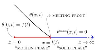
(a)

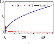
(b)

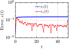
(c)

Figure 3: (a) Schematic of 1D one-phase Stefan problem. (b) Numerical response of the melting front to a constant temperature forcing $\theta(0,t)=f(t)=1$ at the fixed end $x=0$ along with (c) the instantaneous pointwise error.

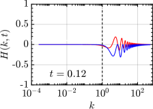
(a)

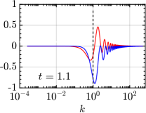
(b)

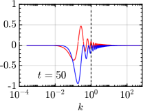
(c)

Figure 4: Evolution of real (red)/imaginary (blue) parts of the history function $H(k,t)$ in the truncated $k-$domain $k\in[0,500]$ at different time instances for the single-phase Stefan problem subject to constant temperature forcing $(f(t)=1)$ at the fixed end $x=0$. $M=2000$ Chebyshev nodes were used to accurately compute the integral of the highly oscillatory history function.

3 Conclusions

We have described a Markovian embedding procedure for evolutionary equations with memory effects, which critically relied on the spectral representation of the memory kernel. We have explicitly shown the embedding procedure for two physical models, namely the one-dimensional walking droplet and the single-phase Stefan problem. In both cases, the memory kernel is a nonlinear function of the underlying state variable.

Physical processes inherently follow Markovian dynamics when described adequately by all the driving state variables. The non-Markovian description of the evolution of an isolated state variable, such as in Eqs. (4), (8), is often the result of “integrating out” the effects of “environment” comprising other state variables. While identifying these integrated physical variables may not always be feasible, our Markovian embedding procedure provides an alternative mathematical reconstruction of the Markovian dynamics.

From a computational standpoint, a Markovian representation ensures that the numerical evolution of the corresponding time-discretized system incurs a time-independent cost. This is in contrast with the standard approaches for memory-dependent systems, where the computational cost grows with time. It is important to recognise that our Markovian embedding procedure comes at the cost of solving an additional local-in-time equation for the history function, which is an infinite-dimensional object. An accurate finite-dimensional approximation of the function depends on the behaviour of $H(k,t)$ in the spectral space. In this regard, the two model problems discussed here demonstrate the extreme scenarios: the Stefan problem required a higher-dimensional approximation of the history function, comprising thousands of spectral variables, while the walker problem allowed a lower-dimensional approximation, with only a few tens of spectral variables for an accurate representation of the history function.

References

- Lovalenti and Brady (1993) P. M. Lovalenti, J. F. Brady, The hydrodynamic force on a rigid particle undergoing arbitrary time-dependent motion at small reynolds number, J. Fluid Mech. 256 (1993) 561–605.
- Oza et al. (2013) A. U. Oza, R. R. Rosales, J. W. M. Bush, A trajectory equation for walking droplets: hydrodynamic pilot-wave theory, J. Fluid Mech. 737 (2013) 552–570.
- Peng and Schnitzer (2023) G. G. Peng, O. Schnitzer, Weakly nonlinear dynamics of a chemically active particle near the threshold for spontaneous motion ii. history-dependent motion, Phys. Rev.Fluids 8 (2023) 033602.
- Stefan (1891) J. Stefan, Ueber die theorie der eisbildung, insbesondere über die eisbildung im polarmeere, Annalen der Physik 278 (1891) 269–286.
- Fokas and Pelloni (2012) A. S. Fokas, B. Pelloni, Generalized Dirichlet-to-Neumann map in time-dependent domains, Stud. Appl. Math. 129 (2012) 51–90.
- Mann and Wolf (1951) W. R. Mann, F. Wolf, Heat transfer between solids and gasses under nonlinear boundary conditions, Q. Appl. Math. 9 (1951) 163–184.
- Keller and Olmstead (1972) J. B. Keller, W. E. Olmstead, Temperature of a nonlinearly radiating semi-infinite solid, Q. Appl. Math. 29 (1972) 559–566.
- Olmstead and Handelsman (1976) W. E. Olmstead, R. A. Handelsman, Asymptotic solution to a class of nonlinear volterra integral equations. II, SIAM J. Appl. Math. 30 (1976) 180–189.
- Dafermos (1970) C. Dafermos, Asymptotic stability in viscoelasticity, Archive for Rational Mechanics and Analysis 37 (1970) 297–308.
- Jaganathan et al. (2023) D. Jaganathan, R. Govindarajan, V. Vasan, Explicit Runge-Kutta algorithm to solve non-local equations with memory effects: case of the Maxey-Riley-Gatignol equation (2023). arXiv:2308.09714.
- Couder et al. (2005) Y. Couder, S. Protière, E. Fort, A. Boudaoud, Dynamical phenomena: Walking and orbiting droplets, Nature 437 (2005) 208–208.
- Valani et al. (2019) R. N. Valani, A. C. Slim, T. Simula, Superwalking droplets, Phys. Rev. Lett 123 (2019) 024503.
- Bush and Oza (2020) J. W. M. Bush, A. U. Oza, Hydrodynamic quantum analogs, Reports on Progress in Physics 84 (2020) 017001.
- Bacot et al. (2019) V. Bacot, S. Perrard, M. Labousse, Y. Couder, E. Fort, Multistable free states of an active particle from a coherent memory dynamics, Phys. Rev. Lett 122 (2019) 104303.
- Faraday (1831) M. Faraday, On a peculiar class of acoustical figures; and on certain forms assumed by groups of particles upon vibrating elastic surfaces, Philosophical Transactions of the Royal Society London Series I 121 (1831) 299–340.
- Durey et al. (2020) M. Durey, S. E. Turton, J. W. M. Bush, Speed oscillations in classical pilot-wave dynamics, Proceedings of the Royal Society of London Series A: Mathematical, Physical and Engineering Sciences 476 (2020) 20190884.
- Valani et al. (2021) R. N. Valani, A. C. Slim, D. M. Paganin, T. P. Simula, T. Vo, Unsteady dynamics of a classical particle-wave entity, Phys. Rev. E 104 (2021) 015106.
- Moláček (2013) J. Moláček, Bouncing and walking droplets : towards a hydrodynamic pilot-wave theory, Ph.D. thesis, Massachusetts Institute of Technology, 2013.
- Durey (2020) M. Durey, Bifurcations and chaos in a Lorenz-like pilot-wave system, Chaos 30 (2020) 103115.
- Valani (2022) R. N. Valani, Lorenz-like systems emerging from an integro-differential trajectory equation of a one-dimensional wave–particle entity, Chaos 32 (2022).
- Guenther and Lee (2012) R. Guenther, J. Lee, Partial Differential Equations of Mathematical Physics and Integral Equations, Dover Books on Mathematics, Dover Publications, 2012.
- Cox and Matthews (2002) S. Cox, P. Matthews, Exponential time differencing for stiff systems, J. Comput. Phys. 2 (2002) 430–455.
- Mitchell and Vynnycky (2009) S. Mitchell, M. Vynnycky, Finite-difference methods with increased accuracy and correct initialization for one-dimensional Stefan problems, Appl. Math. Comput. 215 (2009) 1609–1621.