Strong Bow Shocks: Turbulence and An Exact Self-Similar Asymptotic

Abstract

We show that strong bow shocks are turbulent and non-universal near the head, but asymptote to a universal steady, self-similar, and analytically solvable flow in the downstream. The turbulence is essentially 3D, and has been confirmed by a 3D simulation. The asymptotic behavior is confirmed with high resolution 2D and 3D simulations of a cold uniform wind encountering both a solid spherical obstacle and stellar wind. This solution is relevant in the context of: (i) probing the kinematic properties of observed high-velocity compact bodies — e.g., runaway stars and/or supernova ejecta blobs — flying through the interstellar medium; and (ii) constraining stellar bow shock luminosities invoked by some quasi-periodic eruption (QPE) models.

.5

1 Introduction

Astrophysical bow shocks are ubiquitous; they form at stars flying supersonically through the interstellar medium (e.g., van Buren & McCray, 1988; Kobulnicky et al., 2010; Mackey et al., 2012, 2015), around planets (see e.g., Tsurutani & Stone, 1985; Treumann & Jaroschek, 2008, for comprehensive reviews), or colliding wind binaries (e.g., Stevens et al., 1992; Myasnikov et al., 1998; Gayley, 2009; Sasaki et al., 2023), to name a few scenarios.

Astrophysical bow shocks can be magnetized and collisionless, but we will study them in the hydrodynamics approximation. Conserved mass, momentum, and energy makes the hydrodynamics approximation meaningful even outside of its precise domain of applicability.

Wilkin (1996, hereafter W96) gives an exact analytic solution for a stellar wind bow shock “without pressure”, corresponding to infinitely efficient cooling. In the far downstream, W96’s bow shock asymptotes to $z\propto r^{3}$. The W96 solution was later generalized to wind-wind shocks including the case where one of the winds is anisotropic (Tarango-Yong & Henney, 2018).

To the best of our knowledge, Yalinewich & Sari (2016, hereafter YS16) were the first to offer a theory of the non-radiative bow shock with infinite Mach number. To find the shape of the bow shock, YS16 propose the thought experiment: replace an object moving through a cold medium by a properly timed series of explosions. Assuming that the resulting blast waves are sandwiched between each other, YS16 get the bow shock shape $z\propto r^{2}$. YS16 was an important motivation for us, although formally speaking we do not use any of their results. Unlike YS16, we derive an exact self-similar asymptotic for the strong bow shock, and we also discuss turbulence that necessarily manifests near the obstacle head.

Our main interest is the astrophysically relevant case of a bow shock created by the stellar wind, although we also consider a rigid obstacle. In this work, we prove that the non-relativistic non-radiative bow shock asymptotes to $z\propto r^{2}$ and give the exact expressions for the flow in the far asymptotic. We confirm these exact expressions by high-resolution hydrodynamical simulations. We also prove that a bow shock from the stellar wind is turbulent near the head. The turbulence is essentially 3D. We confirm the turbulence by 3D hydrodynamical simulations.

Theoretical considerations are in Section 2. Numerical results are in Section 3. We conclude and discuss the relevance of our work in Section 4.

2 Theory

One would think that a mathematical description of a bow shock created by a stellar wind is insurmountably difficult. There are at least three surfaces of discontinuity in the flow: two shocks and one tangential discontinuity , see Figure 1. The shapes of these singular surfaces are determined by the flow in between them, and the flow itself depends on the shapes of the singular surfaces. “Mathematically such problems are altogether inaccessible to our present analytical techniques” wrote von Neumann, before presenting his exact solution of the strong explosion problem (von Neumann, 1947).

Moreover, we will prove that the bow shock is turbulent, and surely one doesn’t have the mathematical description of turbulence, yet — in the far downstream — the flow admits an exact solution for the same reason that the strong explosion problem admits an exact solution at large time after the explosive material has transferred most of its energy to the atmospheric gas.

In Section 2.1 we prove that the bow shock is turbulent. In Section 2.2 we derive the exact far-downstream asymptotic. The theoretical considerations presented below are very simple – hard to believe they do work, given that “such problems are altogether inaccessible”, but Section 3 fully confirms this simple theory by direct high-resolution axisymmetric 2D and full 3D numerical simulations.

2.1 Turbulence

The bow shock must be turbulent near the head, at least if a bow shock is created by the stellar wind. Here is the proof.

Assume that the flow is laminar. Then, in the frame of the star, the flow is steady. In this frame, the cold stellar wind collides with the cold interstellar medium (ISM) wind, Figure 1. Before colliding, the two winds shock and pressurize. The pressurized ISM and the pressurized stellar gas touch each other along a steady tangential discontinuity surface. The gas velocity normal to the tangential discontinuity is zero, the pressure doesn’t jump across the discontinuity, but the tangential velocity does jump. In three space dimensions, even a finite-Mach tangential discontinuity is unstable. According to (Landau & Lifshitz, 1959, section 84, problem 1), this was shown by Syrovatskii (1954). In an ideal inviscid gas, the instability of the tangential discontinuity manifests as turbulence. The instability and the resulting turbulence are essentially 3D; we will need a 3D simulation to confirm turbulence in Section 3.

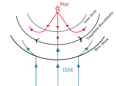
Figure 1: Pictorial depiction of a stellar wind colliding with the cold interstellar medium, which forms a bow shock and inner shock with a tangential discontinuity separating the two shocks.

2.2 Asymptotically Self-Similar Bow Shocks

We have just proved that the flow must be turbulent near the head of the bow shock. Nevertheless we will now assume that turbulence dies out in the far downstream, and the flow becomes steady.

Equations of steady gas flow – continuity, Euler, and adiabaticity – for the density $\rho$, velocity ${\bf v}$, and sound speed $c$ ($c^{2}=\gamma\frac{p}{\rho}$, $p$ is the pressure) are

$$\nabla\cdot(\rho{\bf v})=0,$$ (1)

$$\gamma\rho({\bf v}\cdot\nabla){\bf v}+\nabla(\rho c^{2})=0,$$ (2)

$$({\bf v}\cdot\nabla)\left(\ln c-\frac{\gamma-1}{2}\ln\rho\right)=0,$$ (3)

where $\gamma$ is the adiabatic index.

Assume an axisymmetric flow without a swirl: in cylindrical coordinates $(r,\phi,z)$, the velocity vector is ${\bf v}=(u,0,v)$ and $\rho$, $c$, $u$, $v$ are functions of $r$ and $z$ only. The shock is at $r=R(z)$. The incoming flow is $\rho=1$, $c=0$, $u=0$, and $v=1$.

Equations (1) – (3) should then be solved in the domain $r<R(z)$ with the boundary conditions at $r=R(z)$ which follow from the shock jump conditions:

$$\rho=\frac{\gamma+1}{\gamma-1},$$ (4)

$$c=\frac{\sqrt{2\gamma(\gamma-1)}}{\gamma+1}\frac{R^{\prime}}{\sqrt{1+R^{\prime 2}}},$$ (5)

$$u=\frac{2}{\gamma+1}\frac{R^{\prime}}{1+R^{\prime 2}},$$ (6)

$$v=\frac{1+\frac{\gamma-1}{\gamma+1}R^{\prime 2}}{1+R^{\prime 2}}.$$ (7)

As written, Equations (1) – (3) with the boundary conditions (4) – (7) have no meaningful solutions, because the obstacle creating the bow shock is not specified. We will show, however, that at $z\rightarrow+\infty$ a self-similar non-singular asymptotic solution does exist. Namely, for $z\rightarrow+\infty$, one can use the following expansion in small $R^{\prime}$:

$$\rho=\rho_{0}(\xi)+\rho_{2}(\xi)R^{\prime 2}+\rho_{4}(\xi)R^{\prime 4}+...,$$ (8)

$$c=c_{1}(\xi)R^{\prime}+c_{3}(\xi)R^{\prime 3}+c_{5}(\xi)R^{\prime 5}+...,$$ (9)

$$u=u_{1}(\xi)R^{\prime}+u_{3}(\xi)R^{\prime 3}+u_{5}(\xi)R^{\prime 5}+...,$$ (10)

$$v=v_{0}(\xi)+v_{2}(\xi)R^{\prime 2}+v_{4}(\xi)R^{\prime 4}+...,$$ (11)

where

$$\xi\equiv\frac{r}{R(z)}$$ (12)

is the self-similarity variable.

These expressions are consistent with the jump conditions Equations (4) – (7). When Equations (8) – (11) are plugged into the gas flow equations Equations (1) – (3), one gets a hierarchy of equations for successive orders. The calculation is straightforward, with only one subtlety. The operator $\partial_{z}$, when applied to Equations (8) – (11), generates $R^{\prime\prime}$. The asymptotic expansion Equations (8) – (11) will be consistent with the steady flow Equations (1) – (3) iff one can also expand

$$\frac{RR^{\prime\prime}}{R^{\prime 2}}=b_{0}+b_{1}R^{\prime 2}+b_{2}R^{\prime 4}+...,$$ (13)

where $b$ are constants.

Below we consider only the leading-order solution, but we must note that the first subleading order may also be interesting. At the first subleading order, a bow shock created by the rigid obstacle differs from a bow shock created by the stellar wind. And bow shocks created by different stellar wind velocities differ from each other.

At the leading order, all strong bow shocks have the same asymptotic. To leading order,

$$v=1.$$ (14)

This is because, to leading order, $v=1$ at the shock and, to leading order, the Bernoulli equation gives $v={\rm const}$ along a streamline. Thus, asymptotically the bow shock slows down to the ISM velocity. This doesn’t mean that the bow shock becomes “invisible” in the far downstream. Our bow shock is strong, so the maximal density at any fixed arbitrarily large $z$ is still a factor of a few (4 for $\gamma=5/3$) greater than the unperturbed ISM density.

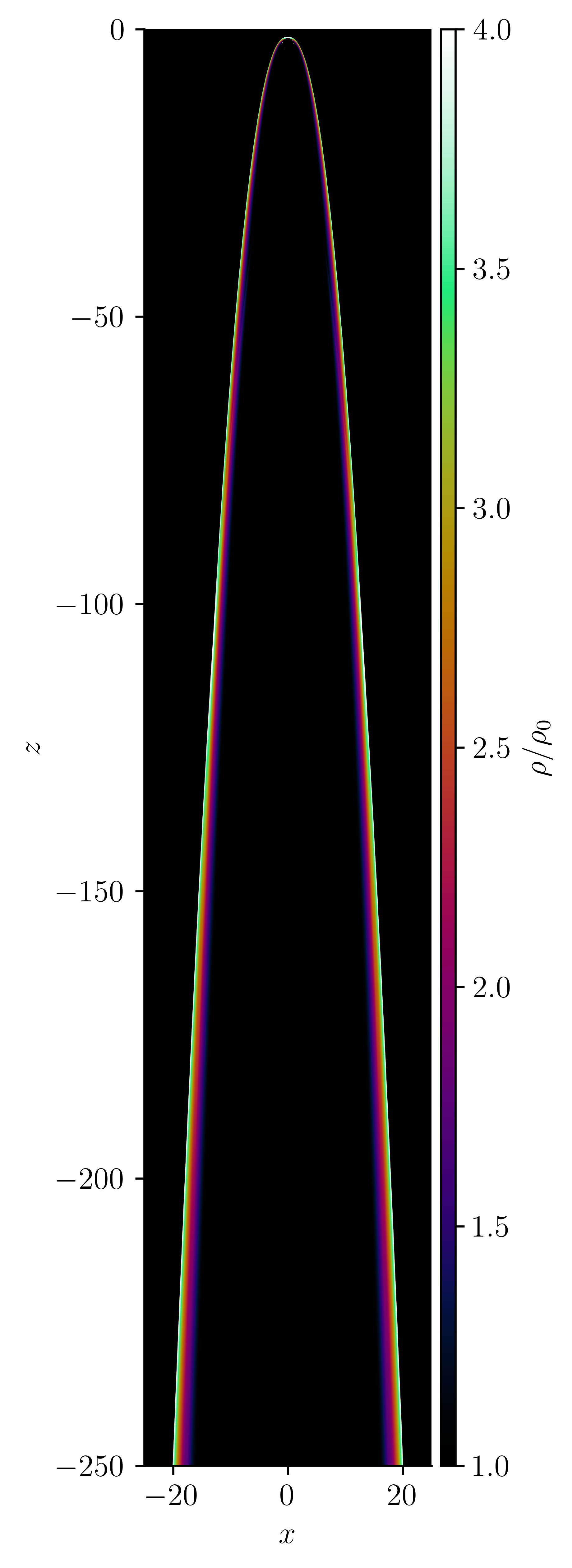
Figure 2: The full structure of the bow show for a rigid obstacle plotted at $t=1,000$. The bow shock wings extend to a maximum of 20 characteristic radii from the symmetry axis.

With $v=1$, the system (1) – (3) reads

$$\partial_{z}\rho+\frac{1}{r}\partial_{r}(r\rho u)=0,$$ (15)

$$(\partial_{z}+u\partial_{r})u=-\frac{1}{\gamma\rho}\partial_{r}(\rho c^{2}),$$ (16)

$$(\partial_{z}+u\partial_{r})\left(\ln c-\frac{\gamma-1}{2}\ln\rho\right)=0.$$ (17)

The boundary conditions, to leading order, are

$$\rho=\frac{\gamma+1}{\gamma-1},$$ (18)

$$c=\frac{\sqrt{2\gamma(\gamma-1)}}{\gamma+1}R^{\prime},$$ (19)

$$u=\frac{2}{\gamma+1}R^{\prime}.$$ (20)

Equations (15) – (20) are isomorphic to a cylindrically symmetric blast wave; $z$ plays the role of time. An exact solution can immediately be deduced, analogous to the Sedov-von Neumann solution (Landau & Lifshitz (1959), section 106):

$$R(z)\propto z^{1/2},$$ (21)

$$\begin{aligned} \rho&=G(\xi)&u&=R^{\prime}U(\xi)\xi&c=R^{\prime}C(\xi)\xi\end{aligned}$$ (22)

$$\xi^{2}=\frac{4}{\gamma^{2}-1}\left(\frac{\gamma-1}{\gamma(\gamma+1)}\right)^{\frac{1}{\gamma}}\frac{(U-\frac{1}{\gamma})^{(1-\frac{1}{\gamma})}}{U(\frac{2}{\gamma}-U)},$$ (23)

$$\begin{split}G=\frac{\gamma+1}{\gamma-1}\left(\frac{\gamma(\gamma+1)}{\gamma-1}\right)^{\frac{1}{\gamma}}\left(\frac{\gamma(\gamma-1)}{2}\right)^{\frac{2}{2-\gamma}}\\ \times\left(U-\frac{1}{\gamma}\right)^{\frac{1}{\gamma}}\left(\frac{\frac{2}{\gamma}-U}{1-U}\right)^{\frac{2}{2-\gamma}},\end{split}$$ (24)

$$C^{2}=\frac{\gamma-1}{2}\frac{U^{2}(1-U)}{U-\frac{1}{\gamma}}.$$ (25)

We will see that these analytic expressions do accurately describe the far downstream of various bow shocks: created by the rigid obstacle, or by the stellar winds with different stellar wind velocity to the star velocity ratios.

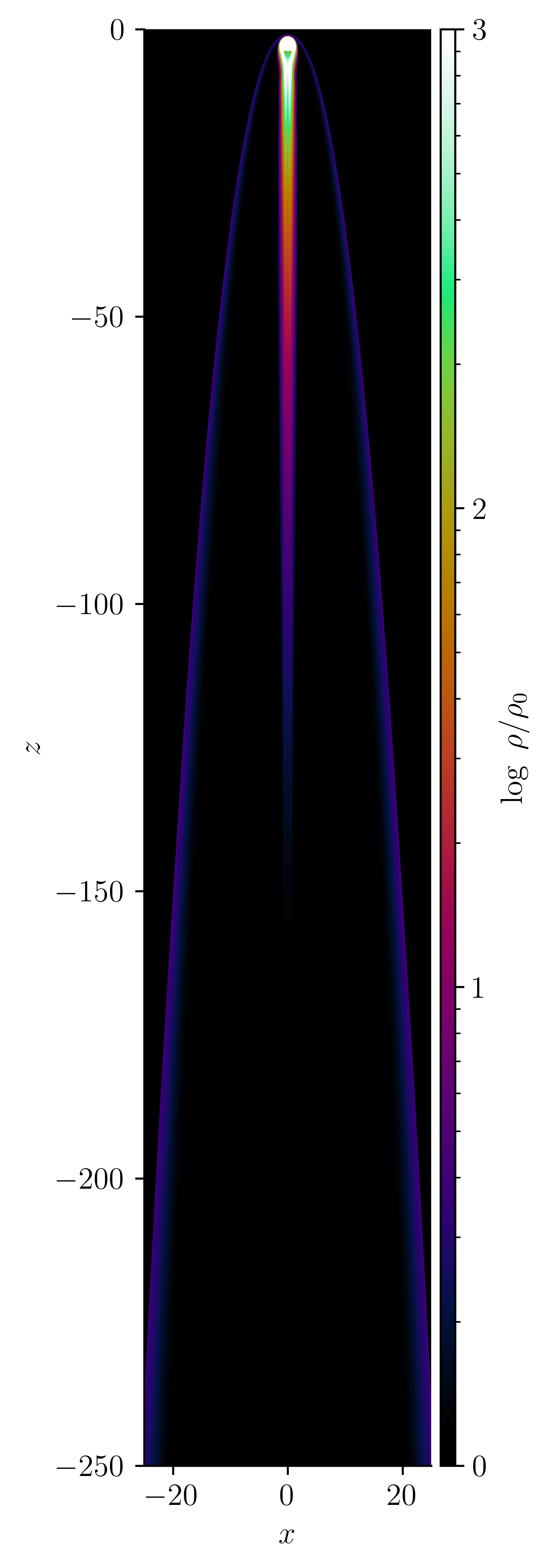
Figure 3: The full structure of the bow show for an obstacle with $v_{\rm wind}=0.1$ plotted at $t=1,000$. The bow shock wings are wider than those of the rigid bow shown in Figure 2 due to inner-outer wind interaction.

3 Numerical Setup and Results

3.1 Numerical Setup

The far asymptotic behavior of the bow shock can be solved numerically in 2D axisymmetry since turbulence near the head of the bow shock is washed out in the far downstream. However, turbulence is inherently a 3D phenomenon; therefore, we perform the numerical experiments in 2D to study the self-similar asymptotic discussed in Section 2.2, and we use 3D to investigate the turbulence criteria described in Section 2.1.

We solve the Euler equations in conservative form:

$$\partial_{t}\rho+\nabla\cdot(\rho\textbf{v})=0,$$ (26)

$$\partial_{t}(\rho\textbf{v})+\nabla\cdot(\rho\textbf{v}\otimes\textbf{v}+p\mathbb{I})=0,$$ (27)

$$\partial_{t}(\rho e_{\rm T})+\nabla\cdot[(\rho e_{T}+p)\textbf{v}]=0,$$ (28)

where $e_{\rm T}=p/[\rho(\gamma-1)]+|\textbf{v}|^{2}/2$ is the total specific energy and $\mathbb{I}$ is the identity matrix. We solve Equations (26) – (28) using a second-order Godunov-type GPU-accelerated gas dynamics code entitled SIMBI (DuPont, 2023). The initial condition is an ambient density of $\rho_{\infty}=1$, ambient vertical velocity $v_{\infty}=-1$, and ambient Mach number $M_{\infty}=10^{4}$ with $\gamma=5/3$. The length scale is set by a characteristic obstacle size $\ell=1$. For the rigid obstacle, $\ell$ is just the radius. For the windy obstacles, $\ell$ is the stand-off distance of the outermost shock. All calculations are done in the rest frame of the obstacle.

We first compute the solution for the solid obstacle. To achieve this, we invoke the immersed boundary method as described in Peskin (2002) where we place a spherical and impermeable boundary surface on top of the grid. This method perfectly captures a rigid body to avoid erroneous ablation effects and Rayleigh-Taylor instabilities. For the wind, we continuously inject mass into a volume such that the stand-off density is $\rho_{\rm s}>\rho_{\infty}(v_{\infty}/v_{\rm wind})^{2}$, where $v_{\rm wind}$ is the ballistic wind velocity. Let $\mathcalligra{r}\,=\sqrt{r^{2}+(z-z_{0})^{2}}$ where $z_{0}$ is the obstacle’s vertical offset, then the wind is

$$\rho_{\rm wind}(\mathcalligra{r}\,\leq\ell)=\rho_{\rm s}(\mathcalligra{r}\,/\ell)^{-2}.$$ (29)

As a parameter study, we investigate the set of wind speeds $v_{\rm wind}=\{0.1,1,10\}$ and their impacts on the far downstream flow.

In 2D, we use an axisymmetric cylindrical mesh with square zones. The vertical domain spans $z\in[0,-250]$ and the radial domain spans $r\in[0,25]$. We ensure at least 102 zones across the obstacle’s cross section, which implies a resolution of $12,800$ vertical zones by 1,280 radial zones. We choose $z_{0}=-2.5$. We run all simulations until a time $t=1,000$ to ensure statistical saturation. Simulations use the generalized minmod slope limiter with $\theta_{\rm PLM}$, a numerical diffusivity factor, set to 1.5 for near-minimal diffusion and more robust preservation of contact surfaces.

As a check for theoretical robustness, we revisit this calculation in full 3D. A limitation of 3D is that we cannot feasibly resolve a Cartesian grid of $12,800\times 2560\times 2560$ zones, so we instead simulate the windy obstacles with $v_{\rm wind}=\{0.1,1\}$ on a coarse-grained 3D grid. We will use this as a litmus test to: (a) see whether there are differences in the saturated flow when going from 2D to 3D; and (b) investigate the assertion made in Section 2.1 that the tangential discontinuity is turbulent near the head of the obstacle. For (a) we ensure 20 zones across the obstacle cross section on a grid that spans $z\in[0,-40]$ and $x,y\in[-20,20]$. For (b) we ensure 200 zones across the obstacle cross section on a grid that spans $z\in[0,-4]$ and $x,y\in[-2,2]$.

3.2 Results

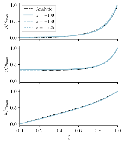
Figure 4: Shown are radial slices of $\rho,p,$ and $u$ at time $t=1,000$ plotted as functions of the self-similarity variable $\xi$ for the rigid obstacle. $\xi=1$ marks the location of the strong bow shock. The dash-dotted black curve marks the theoretical prediction. The blue solid, dashed, and dotted blue curves mark the simulation results at $z=-100,-150,$ and $-225$.

In Figures 2 and 3 we plot the two edge cases considered in this work. Namely, the full structure of the bow shock for the rigid body and the windiest body, i.e, $v_{\rm wind}=0.1$, respectively. In Figure 2 we see the density field behind the rigid body perfectly evacuated, a testament to the robustness of the immersed boundary method invoked to model the boundary layer. In Figure 3, the density field only approaches that of the ambient field at a characteristic radius of $z=-150$. This hints at the fact that the windy obstacles approach the asymptotic solutions slower than the perfectly rigid obstacle since the downstream is polluted by turbulent streams of ablated material.

Moreover, the self-similar theory and numerical simulation show near perfect agreement for the rigid body as shown by Figure 4. There, we plot the quantities $\rho$, $p$, and $u$ as functions of the self-similar variable, $\xi$. We consider $100\ell$ as the nominal threshold for the far downstream and plot each hydrodynamic quantity in logarithmic intervals further downstream to better showcase the self-similar nature of the bow shock extent.

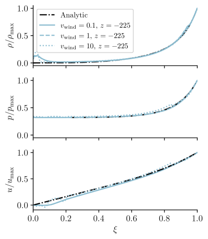
Figure 5: Shown are radial slices of $\rho,p,$ and $u$ at time $t=1,000$ plotted as functions of the self-similarity variable $\xi$ for the windy obstacles. $\xi=1$ marks the location of the strong bow shock. The dash-dotted black curve marks the theoretical prediction. The blue solid, dashed, and dotted curves mark the simulation results for obstacles with wind speeds 0.1, 1, and 10, respectively. All values are plotted at $z=-225$.

Since in reality, the more realistic body flying through the ISM is likely a star with some wind, we plot in Figure 5 $\rho$, $p$, and $u$ for the wind speeds $v_{\rm wind}=\{0.1,1,10\}$ at a fixed distance of $225\ell$. Although some turbulence is present in the far downstream as evidenced by the density bumps near the axis, the overall structure of the bow shock shape still matches nicely with the exact theory derived in the previous section.

The 3D simulations shown in Figure 6 are of the windy obstacles with $v_{\rm wind}=0.1$ in panel (a) and $v_{\rm wind}=1$ in panel (b). Though the 3D simulations were performed with a coarser resolution than the 2D axisymmetric case, panel (a) still shows the same characteristics of the high resolution 2D cases, i.e., the gradual dissipation of the wind material along the axis of the obstacle. Furthermore, panel (b) is a zoomed in region very near the obstacle with $v_{\rm wind}=1$, and we can see the forward shock is relatively stable while axisymmetry is broken by the turbulent contact discontinuity just as we discussed in Section 2.1. Thus, our theory of non-magnetic astrophysical bow shocks is supported by a numerical experiment.

4 Discussion

Figure 6: The bow shock with infinite Mach number when done in full 3D. We plot $v_{\rm wind}=0.1$ case in panel (a) at $t=1,000$ and $v_{\rm wind}=1$ in panel (b). In panel (a) we plot the logarithm of the density field, which shows similar signs of decay along the axis as depicted in the higher resolution 2D runs. In panel (b) we plot the density field for an obstacle with $v_{\rm wind}=1$. The forward shock is relatively stable, but behind it lies the unstable tangential discontinuity between the inner and outer winds. The instability manifest as turbulence as predicted in Section 2.1.

This work has shown that the far asymptotic structure of the bow shock with infinite Mach number is self-similar and analytic. After derivation of the exact asymptotic solution, we confirm the theory with high-resolution hydrodynamical simulations for a rigid obstacle and a windy obstacle. The rigid obstacle shows perfect agreement with the theory. The windy obstacle shows rough agreement with the theory, but this is to be expected since the presence of an inner wind introduces turbulence.

Although inspired by the work of YS16, we have independently developed an exact, analytic solution to the bow shock with infinite Mach number without making any assumptions about the resultant solid of revolution a priori. Due to its exactness and more direct experimental validation, we suggest that our self-similar bow shock theory is more robust methodologically than what is described in YS16.

Having constructed and verified this theory expounding the asymptotic shape of non-magnetic astrophysical bow shocks, the astrophysical implications can be quite expansive. For example, a current theory explaining the sources behind quasi-periodic eruptions (QPEs; Miniutti et al., 2019; Giustini et al., 2020; Arcodia et al., 2021; Chakraborty et al., 2021) are stars that plunge into active galactic nuclei (AGN; e.g., Lu & Quataert, 2023; Tagawa & Haiman, 2023). The supersonic star creates a bow shock whose thermal energy is radiation dominated and this model is used to explain the radiative properties of some QPEs. In the future, we plan to utilize our theory to explore the fundamental problem of stars plunging through AGN disks in order to glean some of the physics of the stellar entry and exit. This should provide constraints on the á la mode QPE models proposed.

The authors thank Tamar Faran, Yuri Levin, and Zoltan Haiman for useful discussions. MD acknowledges a James Author Fellowship from NYU’s Center for Cosmology and Particle Physics, and thanks the LSST-DA Data Science Fellowship Program, which is funded by LSST-DA, the Brinson Foundation, and the Moore Foundation; his participation in the program has benefited this work.

References

- Arcodia et al. (2021) Arcodia, R., Merloni, A., Nandra, K., et al. 2021, Nature, 592, 704, doi: 10.1038/s41586-021-03394-6
- Chakraborty et al. (2021) Chakraborty, J., Kara, E., Masterson, M., et al. 2021, ApJ, 921, L40, doi: 10.3847/2041-8213/ac313b
- DuPont (2023) DuPont, M. 2023, SIMBI: 3D relativistic gas dynamics code, Astrophysics Source Code Library, record ascl:2308.003. http://ascl.net/2308.003
- Gayley (2009) Gayley, K. G. 2009, ApJ, 703, 89, doi: 10.1088/0004-637X/703/1/89
- Giustini et al. (2020) Giustini, M., Miniutti, G., & Saxton, R. D. 2020, A&A, 636, L2, doi: 10.1051/0004-6361/202037610
- Kobulnicky et al. (2010) Kobulnicky, H. A., Gilbert, I. J., & Kiminki, D. C. 2010, ApJ, 710, 549, doi: 10.1088/0004-637X/710/1/549
- Landau & Lifshitz (1959) Landau, L. D., & Lifshitz, E. M. 1959, Fluid mechanics (Oxford: Pergamon Press)
- Lu & Quataert (2023) Lu, W., & Quataert, E. 2023, MNRAS, 524, 6247, doi: 10.1093/mnras/stad2203
- Mackey et al. (2015) Mackey, J., Gvaramadze, V. V., Mohamed, S., & Langer, N. 2015, A&A, 573, A10, doi: 10.1051/0004-6361/201424716
- Mackey et al. (2012) Mackey, J., Mohamed, S., Neilson, H. R., Langer, N., & Meyer, D. M. A. 2012, ApJ, 751, L10, doi: 10.1088/2041-8205/751/1/L10
- Miniutti et al. (2019) Miniutti, G., Saxton, R. D., Giustini, M., et al. 2019, Nature, 573, 381, doi: 10.1038/s41586-019-1556-x
- Myasnikov et al. (1998) Myasnikov, A. V., Zhekov, S. A., & Belov, N. A. 1998, MNRAS, 298, 1021, doi: 10.1046/j.1365-8711.1998.01666.x
- Peskin (2002) Peskin, C. S. 2002, Acta Numerica, 11, 479–517, doi: 10.1017/S0962492902000077
- Sasaki et al. (2023) Sasaki, M., Robrade, J., Krause, M. G. H., et al. 2023, arXiv e-prints, arXiv:2312.03346, doi: 10.48550/arXiv.2312.03346
- Stevens et al. (1992) Stevens, I. R., Blondin, J. M., & Pollock, A. M. T. 1992, ApJ, 386, 265, doi: 10.1086/171013
- Syrovatskii (1954) Syrovatskii, S. I. 1954, Zh. Eksp. Teor. Fiz. (In Russian), 27, 121
- Tagawa & Haiman (2023) Tagawa, H., & Haiman, Z. 2023, MNRAS, 526, 69, doi: 10.1093/mnras/stad2616
- Tarango-Yong & Henney (2018) Tarango-Yong, J. A., & Henney, W. J. 2018, MNRAS, 477, 2431, doi: 10.1093/mnras/sty669
- Treumann & Jaroschek (2008) Treumann, R. A., & Jaroschek, C. H. 2008, arXiv e-prints, arXiv:0808.1701, doi: 10.48550/arXiv.0808.1701
- Tsurutani & Stone (1985) Tsurutani, B. T., & Stone, R. G. 1985, Geophysical Monograph Series, 35, doi: 10.1029/GM035
- van Buren & McCray (1988) van Buren, D., & McCray, R. 1988, ApJ, 329, L93, doi: 10.1086/185184
- von Neumann (1947) von Neumann, J. 1947, Los Alamos National Lab, 2000, 27. https://apps.dtic.mil/sti/citations/ADA384954
- Wilkin (1996) Wilkin, F. P. 1996, ApJ, 459, L31, doi: 10.1086/309939
- Yalinewich & Sari (2016) Yalinewich, A., & Sari, R. 2016, ApJ, 826, 177, doi: 10.3847/0004-637X/826/2/177