Joining Entities Across Relation and Graph with a Unified Model

Abstract.

This paper introduces $\mathsf{RG}$ (Relational Genetic) model, a revised relational model to represent graph-structured data in $\mathsf{RDBMS}$ while preserving its topology, for efficiently and effectively extracting data in different formats from disparate sources. Along with: (a) ${\mathsf{SQL_{\delta}}}$, an $\mathsf{SQL}$ dialect augmented with graph pattern queries and tuple-vertex joins, such that one can extract graph properties via graph pattern matching, and “semantically” match entities across relations and graphs; (b) a logical representation of graphs in $\mathsf{RDBMS}$, which introduces an exploration operator for efficient pattern querying, supports also browsing and updating graph-structured data; and (c) a strategy to uniformly evaluate $\mathsf{SQL}$, pattern and hybrid queries that join tuples and vertices, all inside an $\mathsf{RDBMS}$ by leveraging its optimizer without performance degradation on switching different execution engines. A lightweight system, $\mathsf{WhiteDB}$, is developed as an implementation to evaluate the benefits it can actually bring on real-life data. We empirically verified that the $\mathsf{RG}$ model enables the graph pattern queries to be answered as efficiently as in native graph engines; can consider the access on graph and relation in any order for optimal plan; and supports effective data enrichment.

1. Introduction

Data enrichment aims at extracting properties and attributes in different formats from disparate sources, and incorporating additional useful information for users to make insightful and informed decisions, which is highly valued for its increasing practicality in a variety of applications (SEON, 2021; Insights, 2023; Research, 2022, 2018a; Partners, 2023; MMR, 2022; Research and Consulting, 2022; Research, 2018b). In particular, to enrich the semantics of relational data with graph properties and enrich their graph queries with relational predicates, unified data analytics is required for the practitioners to identify the aligned entities across graphs and relations dynamically and join them together.

Example 1.

Below is a recommendation task from a social media company, which maintains: (1) a relational database $\mathcal{D}$ of detailed user portrait and profile, and (2) a graph $G$ of the “follow” among users and the links the users share. The connection between $G$ and $\mathcal{D}$ can be maintained for the vertices and the tuples to be matched together with aligned user id. Meanwhile, the company would also monitor an external database $\mathcal{D}_{E}$ of on-going events from disparate sources, and decide whether to push those news to its users according to their profile and the users they are following.

The company then needs to: (1) match a pattern $P$ in $G$ to find the links shared by both a user and its follower, (2) extract the events from $\mathcal{D}_{E}$ relevant to the shared links, and (3) access the profile of the follower from $\mathcal{D}$ to find whether they would be interested in those events. As demonstrated in Figure 1, $rest_{0}$ can be recommended to $user_{1}$ to try on their new French dishes.

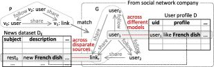
Figure 1. An example hybrid query

The need for unified data analytics is evident in practice to extract value out of the Variety of big data (Russom et al., 2011). More specifically, to effectively and efficiently join the aligned entities across graph and relation according to equivalent value or semantic connection, several questions need to be answered. Is it possible to dynamically enrich relational entities identified by $\mathsf{SQL}$ queries with additional properties of the same entities from graphs? How can we enrich graph queries with relational properties? Can we support these “hybrid” queries in a relational database management system ($\mathsf{RDBMS}$) without switching between relation and graph engines? Is it possible to store graphs in the $\mathsf{RDBMS}$ such that the system is able to conduct graph pattern matching as efficient as a native graph engines (Ma et al., 2016)? How can we efficiently evaluate the hybrid queries with an enlarged unified plan space by leveraging the optimizer of the $\mathsf{RDBMS}$?

Several systems have been built atop an $\mathsf{RDBMS}$ by storing graphs as relations (Zhao and Yu, 2017; Zhang et al., 2022; Steer et al., 2017; Jindal et al., 2015; Jindal et al., 2014; Dave et al., 2016; Quamar and Deshpande, 2016; da Trindade et al., 2020; Deshpande, 2018). These systems either translate specific types of graph queries into $\mathsf{SQL}$ and execute the queries via the $\mathsf{RDBMS}$, or extract graph views of relations and conducts graph analytics using another query engine. These methods either incur heavy cost when answering common graph queries, e.g., graph pattern matching since it involves multi-way join, as observed in (Ma et al., 2016); or do not allow users to write declarative queries in their familiar language such as $\mathsf{SQL}$ and do not make use of the sophisticated optimizer of $\mathsf{RDBMS}$, as pointed out by (Hassan et al., 2018a). While some systems, e.g., (Hassan et al., 2018a), combine the two approaches and uniformly support both, none of the systems support hybrid queries specified in Example 1 to enrich data as demanded by practitioners. In particular, no prior systems are able to dynamically identify an entity $e$ by a tuple returned by an $\mathsf{SQL}$ query, extract the properties of the same entity encoded in a graph, and enrich $e$ with the properties as additional attributes, all inside the $\mathsf{RDBMS}$.

Contributions & organization. In light of these, this paper introduces $\mathsf{RG}$ (Relational Genetic) model to uniformly represent graphs in $\mathsf{RDBMS}$, along with an implementation of it, $\mathsf{WhiteDB}$. The novelty of it consists of the following. (a) It supports a dialect of $\mathsf{SQL}$ to dynamically enrich relational entities with additional graph properties of the same entities, and enrich graph pattern matching with relational predicates. This departs from previous works (Zhao and Yu, 2017; Zhang et al., 2022; Steer et al., 2017; da Trindade et al., 2020; Jindal et al., 2015; Jindal et al., 2014; Dave et al., 2016; Quamar and Deshpande, 2016; Deshpande, 2018; Hassan et al., 2018a). (b) It provides a logical representation of graph-structured data in $\mathsf{RDBMS}$, which preserves its topology and provides more efficient operators to conduct graph pattern matching as efficient as a native graph store. (c) The $\mathsf{RG}$ model enables an enlarged unified plan space to uniformly optimize native $\mathsf{SQL}$ queries, graph pattern queries and hybrid queries by fully leveraging the sophisticated query optimizer of the $\mathsf{RDBMS}$, and allow them to be executed all inside $\mathsf{RDBMS}$ without performance degradation. We show the above advantages by empirically evaluating the performance of $\mathsf{WhiteDB}$ with real-life data.

Pattern matching is focused as graph queries in this work, to prove the concept of unified evaluation for hybrid queries (see (ful, 2023)). As surveyed in (Sahu et al., 2020), pattern matching dominates the topics of studies on graph computations, and also have been widely used in social network analysis (Fan et al., 2015), security (Jiang et al., 2010), software engineering (Surian et al., 2010), biology (Royer et al., 2008) and chemistry (Wegner et al., 2006), among other things. Graph pattern matching has also been considered as one of the core functionalities for querying graphs (Angles et al., 2018; Deutsch et al., 2022), and is enabled as a feature in a number of graph query languages, e.g., (Francis et al., 2018; Tin, 2017) and graph databases (Tian, 2023). For data enrichment in particular, pattern queries suffice to identify graph entities and properties by specifying their topological structures. We defer a full treatment of generic graph queries, especially considering the recursive feature (Pérez et al., 2009), to a later paper.

More specifically, we highlight the following.

(1) ${\mathsf{SQL_{\delta}}}$: A dialect of $\mathsf{SQL}$ (Section 2). We propose ${\mathsf{SQL_{\delta}}}$ to support (a) $\mathsf{SQL}$ queries, (b) graph pattern queries, and (c) hybrid of the two by joining entities across relations and graphs. ${\mathsf{SQL_{\delta}}}$ can dynamically join entities: it may identify an entity $e$ by an $\mathsf{SQL}$ query (encoded as a tuple $t$), locate vertex $v$ that represents $e$ in a graph $G$, extract properties of $v$ from $G$ via pattern queries, and enrich $e$ by augmenting $t$ with the graph properties of $v$. That is, it “joins” tuple $t$ and vertex $v$ if they refer to the same entity $e$. Each ${\mathsf{SQL_{\delta}}}$ query returns a relation with deduced schema, and is composable with other ${\mathsf{SQL_{\delta}}}$ queries, just like $\mathsf{SQL}$ queries.

(2) Minor extension of $\mathsf{RDBMS}$ (Section 3). We present the query evaluation workflow enabled by the $\mathsf{RG}$ model, inherited from the counterpart for relational query (Stonebraker et al., 1990; Stonebraker et al., 1976) with few operators incorporated into the logical and physical query plans and corresponding revises on the optimizer. The advantages offered by the $\mathsf{RG}$ model can thus be readily obtained by existing $\mathsf{RDBMS}$ as an extension.

(3) Relational model of graphs (Section 4). The $\mathsf{RG}$ model introduces logical pointers to represent graph-structured data in $\mathsf{RDBMS}$ while preserving its topology, to uniformly manage graph and relational data without cross-model access. It also allows users to (a) query graph-structured data with the same efficiency as the native graph stores, (b) browse the graphs stored in it to formulate queries, and (c) update the graphs, to manage the graph-structured data, without breaking the physical data independence (Stonebraker, 1975).

(4) Uniform query evaluation in $\mathsf{RDBMS}$ (Section 5). The $\mathsf{RG}$ model enables an enlarged unified plan space to optimize $\mathsf{SQL}$ queries, graph pattern queries and hybrid queries, which allows the access on graph and relational data to be considered in any order for a more efficient query plan. The generated query plan can then be executed seamlessly all inside the $\mathsf{RDBMS}$ without performance degradation.

(5) Experimental study (Section 6). We provide an implementation of the proposed $\mathsf{RG}$ model to evaluate the advantages it can actually bring on real-life datasets. We empirically verify the following. On average, (a) Integrating the exploration operator induced by the $\mathsf{RG}$ model into the query evaluation workflow enables $\mathsf{WhiteDB}$ to bring orders-of-magnitude performance improvement to other relational systems, 32500x to PostgreSQL and 112x to DuckDB, and also to achieve a comparable performance, 1.01x, to the most efficient native graph-based algorithm we tested. (b) $\mathsf{WhiteDB}$ can optimize the hybrid query in an enlarged unified plan space to pull the low selectivity join conditions down to the pattern matching process for early pruning and evaluate it seamlessly without involving cross model access. Together, a 13.5x speedup is achieved. (c) $\mathsf{WhiteDB}$ still performs well as the pattern scales, which can achieve 0.91x compared to the native graph algorithms as the patterns reach 7 edges.

We discuss related work in Section 7 and future work in Section 8.

2. Expressing Hybrid Queries in SQL_δ

In this section, we introduce ${\mathsf{SQL_{\delta}}}$, a dialect of $\mathsf{SQL}$ to express native $\mathsf{SQL}$ queries, graph pattern queries and hybrid queries.

Preliminaries. Assume a countably infinite set $\mathbb{V}$ as the underlying domain (Abiteboul et al., 1995). A database schema is specified as ${\mathcal{R}}=(R_{1},\allowbreak\ldots,\allowbreak R_{m})$, where each $R_{i}$ is a relation schema with a fixed set of attributes. A tuple $t$ of $R_{i}$ consists of a value in $\mathbb{V}$ for each attribute of $R_{i}$. A relation of $R_{i}$ is a set of tuples of $R_{i}$. A database $\mathcal{D}$ of ${\mathcal{R}}$ is $(D_{1},\ldots,D_{m})$, where $D_{i}$ is a relation of $R_{i}$ for $i\in[1,m]$ (Abiteboul et al., 1995). Following Codd (Codd, 1979), we assume that each tuple $t$ represents an entity.

A graph is specified as $G=(V,E,L,F_{A})$, where (a) $V$ is a finite set of vertices; (b) $E\subseteq V\times V$ is a set of edges, in which $(v,v^{\prime})$ denotes an edge from vertex $v$ to $v^{\prime}$; (c) function $L$ assigns a label $L(v)$ (resp. $L(e)$) to each $v\in V$ (resp. $e\in E$); and (d) each vertex $v{\in}V$ (resp.  edge $e{\in}E$) carries a tuple $F_{A}(v)=(A_{1}=a_{1},...,A_{n}=a_{n})$ (resp. $F_{A}(e)=(B_{1}=b_{1},\ldots,B_{m}=b_{m})$) of attributes of a finite arity, written as $v.A_{i}=a_{i}$ (resp. $e.B_{i}=b_{i}$), and $A_{i}\neq A_{j}$ (resp. $B_{i}\neq B_{j}$) if $i\neq j$.

We assume the existence of a special attribute $\mathsf{id}$ at each vertex $v$, denoting its vertex identity, such that for any two vertices $v$ and $v^{\prime}$ in $G$, if $v.{\mathsf{id}}=v^{\prime}.{\mathsf{id}}$, then $v$ and $v^{\prime}$ refer to the same entity. Similarly, each edge $e$ is also associated with an $\mathsf{id}$ to indicate edge identity.

Patterns. A graph pattern is defined as $P=(V_{P},E_{P},L_{P})$, where $V_{P}$ (resp. $E_{P}$) is a set of pattern vertices (resp. pattern edges) and $L_{P}$ is a labeling function for $V_{P}$ and $E_{P}$ as above.

Matches. A match of a pattern $P$ in a graph $G$ is a homomorphic mapping $h$ from $V_{P}$ to $V$ such that (a) for each pattern vertex $u\in V_{P}$, $L_{P}(u)=L(h(u))$; and (b) for each pattern edge $e=(u,u^{\prime})\in E_{P}$, there exists an edge $(h(u),h(u^{\prime}))$ in graph $G$ labeled $L_{P}(e)$. By slight abuse of notation, we also denote $(h(u),L_{P}(e),h(u^{\prime}))$ as $h(e)$.

Pattern queries. A graph pattern query is $P[\bar{A}]$, where (a) $P$ is a graph pattern, and (b) $\bar{A}$ is a list of attributes such that each $A_{i}$ in $\bar{A}$ is attached to a pattern vertex or edge in $P$.

We represent the result $P[\bar{A}](G)$ of pattern $P[\bar{A}]$ over graph $G$ as a relation $S$ of schema $R_{P}$ with attributes $\bar{A}$. More specifically, each match $h$ of $P$ in $G$ is encoded as a tuple $s$ in relation $S$, such that each attribute $A_{i}$ in $\bar{A}$ is associated with pattern vertex $u$ (resp. pattern edge $e$), $s[A_{i}]=h(u).A_{i}$ (resp. $s[A_{i}]=h(e).A_{i}$).

Intuitively, besides topological matching, pattern queries extract important properties for entities of interests from the graphs. These are organized in the form of relations with a deducible schema.

RA_δ. We present a dialect of relational algebra ($\mathsf{RA}$), denoted by ${\mathsf{RA_{\delta}}}$. A query of ${\mathsf{RA_{\delta}}}$ has one of the following forms:

$$Q ::= R\ |\ \pi_{\bar{A}}Q\ |\ \sigma_{C}Q\ |\ Q_{1}\bowtie Q_{2}\ |\ Q_{1}\cup Q_{2}\ |\ Q_{1}\setminus Q_{2}\ |\$$

$$P[\bar{A}](G)\ |\ Q_{1}\bowtie_{\delta}Q_{2}.$$

Here (a) $R,\pi,\sigma$, $\bowtie$ , $\cup$ and $\setminus$ denote relation atom, projection, selection and (natural) join, set union and difference, respectively, as in the classic $\mathsf{RA}$ (see (Abiteboul et al., 1995)); (b) $P[\bar{A}](G)$ is a graph pattern query as defined above; it returns a relation of schema $R_{P}$, where $G$ is (the name of) a graph; and (c) $Q_{1}\bowtie_{\delta}Q_{2}$ “joins” two queries according to their semantic connection (see below), denoted by $\delta$-join.

The semantics of $\delta$-join. Suppose that $Q_{1}$ is a relational query $Q$ and $Q_{2}$ is a graph pattern query $P[\bar{A}]$; the cases for joining queries of the same type are similar. Assume that over a database $\mathcal{D}$ of schema ${\mathcal{R}}$, sub-query $Q(\mathcal{D})$ returns a relation $D$ of schema $R_{Q}$ with attributes $\bar{B}$; and over graph $G$, $P[\bar{A}](G)$ returns a relation $S$ of schema $R_{P}$.

The $\delta$-join $Q\bowtie_{\delta}P[\bar{A}](G)$ works as follows: for each result tuple $t\in Q(D)$ and each tuple $s\in S=P[\bar{A}](G)$, if $t$ and $s$ refer to the same real-world entity (with $s[A_{0}]$ as the $\mathsf{id}$), then it returns tuple $t$ augmented with all attributes in $s$ except $A_{0}$. The schema of the result of the $\delta$-join can be readily deduced from $R_{Q}$ and $R_{P}$, i.e., combining attributes $\bar{A}$ and $\bar{B}$ excluding $A_{0}$. This said, graph pattern matching (Angles et al., 2018; Deutsch et al., 2022) and ER (entity resolution) (Altwaijry et al., 2015; Sismanis et al., 2009) are combined here to query across relational and graph data.

Example 1.

The query in Example 1 can be described with ${\mathsf{RA_{\delta}}}$ as: $\mathcal{D}_{E}\bowtie_{\delta}(P[v_{2}.vid](G)\bowtie_{v_{2}.vid=uid}\mathcal{D})$. It consists a pattern query, a join across graph and relational data and a $\delta$-join. Other attributes extracted from pattern query are omitted as a simplification.

Several methods are in place to embed ER in query processing, i.e., to decide whether two tuples refer to the same entity with additional operator at query time, e.g., ETJ/Lineage (Agrawal et al., 2009), polymorphic operators (Altwaijry et al., 2015), hyper-edge (Bhattacharya et al., 2006), parametric simulation (Fan et al., 2022b), entity aggregation with mapping (Sismanis et al., 2009). Such a procedure will be embedded as a black box to return the matched entity pairs from two input relations, which allows all kinds of detailed methods to be adopted here.

SQL_δ. We next present ${\mathsf{SQL_{\delta}}}$. Over database schema ${\mathcal{R}}=(R_{1},\ldots,R_{n})$ and graph $G$, an ${\mathsf{SQL_{\delta}}}$ query has the form:

	select	$A_{1}$, …, $A_{h}$
from	$R_{1}$, …, $R_{n}$,
	$P_{1}[\bar{A}_{1}](G)$, …, $P_{k}[\bar{A}_{k}](G)$,
	$S_{1}\ \mbox{{\bf join}\ }\ P_{1}^{\prime}[\bar{A}_{1}^{\prime}](G)$, …, $S_{m}\ \mbox{{\bf join}\ }\ P_{m}^{\prime}[\bar{A}_{m}^{\prime}](G)$,
	$S_{1}^{\prime}\ \mbox{{\bf map}\ }\ S_{1}^{\prime\prime}$, …, $S_{q}^{\prime}\ \mbox{{\bf map}\ }\ S_{q}^{\prime\prime}$
where	Condition-1 {and —or } …{and —or } Condition-p

Here $S_{1}$, …, $S_{m}$ are either relations of ${\mathcal{R}}$ or ${\mathsf{SQL_{\delta}}}$ sub-queries over ${\mathcal{R}}$ and $G$. An ${\mathsf{SQL_{\delta}}}$ query may embed a normal $\mathsf{SQL}$ query, a pattern query $P_{i}[\bar{A}_{i}](G)$, a value-based hybrid query $S_{j}\ \mbox{{\bf join}\ }\ P_{j}^{\prime}[\bar{A}_{j}^{\prime}](G)$, and a $\delta$-join $S_{k}^{\prime}\ \mbox{{\bf map}\ }\ S_{k}^{\prime\prime}$. Each Condition in the where clause is an $\mathsf{SQL}$ condition over relations $R_{1}$, …, $R_{n}$, and the result relations of pattern queries and $\delta$-joins. Following (Angles et al., 2018; Deutsch et al., 2022; Francis et al., 2018, 2023), users may specify patterns with “ASCII-art” style paths.

Example 2.

The ${\mathsf{RA_{\delta}}}$ query in Example 1 can be written in ${\mathsf{SQL_{\delta}}}$:

		select	$*$   from  (
select  $v0.id$ as $vid_{0}$,  $v2.id$ as $vid_{2}$,  $D.profile$ as $user\_profile$
from  (
select	$v0.id$ as $vid_{0}$,  $v2.id$ as $vid_{2}$  $v1.attr$ as $link\_attr$
match    $(v0:User)\text{-}[e0:Share]\text{->}(v1:Link)$
	$(v2:User)\text{-}[e1:Share]\text{->}(v1:Link)$
	$(v2:User)\text{-}[e2:Follow]\text{->}(v0:User)$
) as $P$  join  $D$ on $P.vid_{0}=D.uid$
) as $P\_R$  map  $D_{E}$

Where pattern $P$ is described with “ASCII-art” style paths.

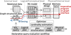
Figure 2. Data representation and query evaluation overview

Usability. ${\mathsf{SQL_{\delta}}}$ retains the capability of query composition (Angles et al., 2018) in $\mathsf{SQL}$, while the extensions it introduces are also all easy for the practitioners to accept: The “ASCII-art” style description of pattern query is widely-recognized in the community of graph query language (Deutsch et al., 2022); The “map” clause for ER can be simply regarded as a special kind of join without specifying conditions (see (ful, 2023) for more).

As will be seen in Section 5, all ${\mathsf{SQL_{\delta}}}$ queries can be evaluated inside an $\mathsf{RDBMS}$ along the same lines as $\mathsf{SQL}$ queries without switching to another system.

3. Hybrid Query Evaluation Overview

The $\mathsf{RG}$ model provides a unified logical level representation of both the relations and graph-structured data from the external (Date, 2000; ste, 1975) view, with a physical data independence to support the declarative hybrid query as shown in Figure 2. As will be seen in Section 5, the $\mathsf{RG}$ model enables an enlarged plan space to uniformly optimize the queries that operate on both graph and relational data, and reduce the overhead incurred by switching between different execution engines with heterogeneous data stores (Tan et al., 2017; Gupta et al., 2016). Moreover, its memory layout can also be efficiently implemented at the physical level.

Workflow. As shown in Figure 2, ${\mathsf{SQL_{\delta}}}$ queries will be processed along exactly the same lines as $\mathsf{SQL}$ queries in $\mathsf{RDBMS}$s (Stonebraker et al., 1990; Stonebraker et al., 1976; Hellerstein et al., 2007). An ${\mathsf{SQL_{\delta}}}$ query $Q_{\delta}$ will be first parsed into a logical plan, then optimized to generate the corresponding physical plan and be executed to get the evaluation result.

We remark the following.

(1) The query evaluation workflow enabled by the $\mathsf{RG}$ model differs from the counterpart in $\mathsf{RDBMS}$s (Graefe, 1993) only in a few simple operators included in the logical and physical plans, and a slight revision of the cost model accordingly. These revises can be incorporated into the relational query evaluation, along with the well-developed techniques (e.g., plan enumeration) (Ramakrishnan et al., 2003), to support hybrid queries.

(2) Along with the model, we provide a lightweight system, $\mathsf{WhiteDB}$, as an implementation to evaluate the actual benefits that the proposed hybrid query evaluation workflow can bring on real-life data, and prove the concept of dynamic data enrichment. A native interface is also supported for procedural graph data access, which allows it to support generic graph computation, not limited to the declarative graph pattern queries. We defer imperative programming for graph computation to fu ture work.

4. Modelling Graphs in Relations

We revise the relational model to store graphs (Section 4.1), present its physical implementation (Section 4.2), and show how to update and browse the graphs maintained in relations (Section 4.3).

4.1. The RG Model

To encode graphs in relations, we propose a simple $\mathsf{RG}$ (Relational Genetic) model. It extends conventional relations with logical pointers, to preserve the topological structures of graphs when stored in relations, and support additional operators for uniform query evaluation across graphs and relations (Section 5).

Assume two disjoint countably infinite sets $\mathbb{V}$ and $\mathbb{P}$, denoting the domains of data values and logical pointers (symbols), respectively.

RG model. Consider a database schema ${\mathcal{R}}=(R_{1},\ldots,R_{m})$. The $\mathsf{RG}$ schema w.r.t. ${\mathcal{R}}$ is ${\mathcal{R}}^{E}=(R_{1}^{E},\ldots,R_{m}^{E})$, in which each $R_{i}^{E}$ extends the conventional schema $R_{i}$ such that the domain of attributes in $R_{i}^{E}$ is $\mathbb{V}\cup\mathbb{P}$ instead of $\mathbb{V}$, i.e., attributes can also be pointers in addition to the plain values, which are references that “virtually link” to a subset of an extended relation.

An extended database $\mathcal{D}^{E}$ of ${\mathcal{R}}^{E}$ is $(D_{1}^{E},\ldots,D_{m}^{E},\phi)$, where (1) $D_{i}^{E}$ is an extended relation, i.e., a set of tuples of $R_{i}^{E}$ for $i\in[1,m]$; and (2) an injective partial reference function $\phi:\bigcup_{i\in[1,m]}\mathcal{P}(D_{i}^{E})\to\mathbb{P}$ maps subsets of an extended relation in $\mathcal{D}^{E}$ to references from the domain ${\mathcal{P}}$. Here $\mathcal{P}(D_{i}^{E})$ is the power set of $D_{i}^{E}$. We also denote by $\psi=\phi^{-1}$ the dereference of a pointer to the specific subset $S$ in $\mathcal{D}^{E}$. This is well-defined since $\phi$ is injective; thus $\psi(\phi(S))=S$.

Regular form. An extended database $\mathcal{D}^{E}$ is in the regular form if: (1) For any two pointers $p_{1}$ and $p_{2}$ in $\mathcal{D}^{E}$, either $\psi(p_{1})\cap\psi(p_{2})=\emptyset$ or $\psi(p_{1})=\psi(p_{2})$; (2) For each extended relation $D_{i}^{E}$ in $\mathcal{D}^{E}$, for each of its attribute $A_{ij}$, there exists an extended relation $D_{ij}^{E}$ in $\mathcal{D}^{E}$, s.t. $\bigcup\{\psi(t[A_{ij}])|t\in D_{i}^{E},t[A_{ij}]\in\mathbb{P}\}\subseteq D_{ij}^{E}$, i.e., all pointers in a same column will not point to different relations. In the sequel, we consider only extended databases in the regular form. This suffices to model graph data.

Remark. The $\mathsf{RG}$ model enhances the classical relational model on its “structural part” (Codd, 1980, 1982) with logical pointers. The pointers are at the logical level, for referencing tuples. Such pointers are along the same lines as foreign keys, similarly for tuple identifiers and the “database pointers” in (Nystrom et al., 2005), for preserving the topology of graph data and for optimizing hybrid/pattern queries.

As will be seen in Section 5, these pointers induce an “exploration” operator into logical query plan and facilitate the evaluation of graph pattern queries, instead of merely supporting semantic optimization (Ramakrishnan and Srivastava, 1994). This allows us to uniformly manage relations and graph data, without cross-model access (Vyawahare et al., 2018; Hassan et al., 2018b; gim, 2021). Moreover, it provides a larger space for optimizing hybrid queries, e.g., pushing relational join conditions down into the pattern matching. In contrast, pointers in $\mathsf{RDBMS}$ (Garcia-Molina and Salem, 1992; Zhang et al., 2015; Wu et al., 2017) are at the physical level and are mainly adopted inside a single tuple, pointing to segments for storing one of its variable-length fields, e.g., VARCHAR in Postgres, or different versions for multi-version concurrency control. Such physical pointers are transparent to logical query plans.

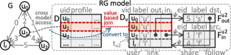
Figure 3. Relations and graphs in the $\mathsf{RG}$ model

Representing graphs. To encode graph $G=(V,E,L,F_{A})$ in the $\mathsf{RG}$ model, we adopt extended relations with the following schemas.

• $\mathsf{V(vid,label,out_{L},in_{L})}$, where each tuple $t$ of $\mathsf{V}$ specifies information related to vertex $v$ with $v.{\mathsf{id}}=t[\mathsf{vid}$]. Here attributes $t[\mathsf{out_{L}}]$ and $t[\mathsf{in_{L}}]$ are pointers to those incoming and outgoing edges incident to $v$, respectively (see below).

• $\mathsf{V^{l}_{A}(vid,A_{1},\ldots,A_{n})}$, for encoding attributes of vertices of a specific type (label) $l$ (Angles et al., 2023).

• $\mathsf{E_{out}(eid,label,dst_{L})}$, where each tuple $t$ of $\mathsf{E_{in}}$ encodes edge $e$ such that $t.[\mathsf{eid}]{=}e.{\mathsf{id}}$, $t[\mathsf{label}]{=}L(e)$ and $t[\mathsf{dst_{L}}]$ is a pointer referencing the destination vertex of $e$ in $\mathsf{V}$-relation.

• $\mathsf{E_{in}(eid,label,src_{L})}$, which is similar to $\mathsf{E_{out}}$ but $\mathsf{src_{L}}$ indicates a pointer referencing the source vertex instead.

• $\mathsf{E_{A}^{l}(eid,B_{1},\ldots,B_{m})}$, for edge attributes with label $l$.

A graph can be converted to such extended relations as follows.

(1) All vertices in $G$ are maintained in a single extended relation $D_{\mathsf{V}}$ of schema $R_{\mathsf{V}}$, by allocating vertex $\mathsf{id}$’s and labels appropriately.

(2) Vertex attributes (resp. edge attributes) are stored in multiple relations $D^{l_{i}}_{\mathsf{V_{A}}}$ (resp. $D^{l_{j}}_{\mathsf{E_{A}}}$) of schema $\mathsf{V^{l_{i}}_{A}}$ (resp. $\mathsf{E^{l_{j}}_{A}}$), one for each $l_{i}$ and $l_{j}$, where the vertex labels $l_{i}$ and edge labels $l_{j}$ are taken from $G$. This is in accordance with the recent attempts on defining schemas for property graphs (Angles et al., 2023) and SQL/PGQ standards (39075, 2023; 9075-16, 2022), where the labels (types) of vertices or edges also indicate allowed attributes. In practice, the number of entity and relationship types in real-life knowledge graphs is relatively small (dbp, 2023b; yag, 2023). When attributes do not exist at some vertices/edges, the corresponding fields are $\mathsf{null}$.

(3) Two relations $D_{\mathsf{out}}$ and $D_{\mathsf{in}}$ of schemas $\mathsf{E_{out}}$ and $\mathsf{E_{in}}$, respectively, maintain the outgoing and incoming edges of vertices. The outgoing (resp. incoming) edges of each vertex $v$ correspond to a subset $F_{\mathsf{out}}^{v}$ (resp. $F_{\mathsf{in}}^{v}$) in $D_{\mathsf{out}}$ (resp. $D_{\mathsf{in}}$). In particular, $F_{\mathsf{in}}^{v}=\emptyset$ (resp. $F_{\mathsf{out}}^{v}=\emptyset$) when $v$ has no incoming edges (resp. outgoing edges).

(4) The pointers and reference function $\phi$ ensure the following: (a) for each $t\in D_{\mathsf{V}}$, $t[\mathsf{in_{L}}]=\phi(F_{\mathsf{in}}^{v})$ and $t[\mathsf{out_{L}}]=\phi(F_{\mathsf{out}}^{v})$ where $t[\mathsf{vid}]=v.{\mathsf{id}}$; (b) $s[\mathsf{dst_{L}}]=\phi(t)$ (resp. $s[\mathsf{in_{L}}]=\phi(t)$) for each $s$ in $D_{\mathsf{out}}$ (resp. $D_{\mathsf{in}}$) and $t$ in $D_{\mathsf{V}}$ with $t[\mathsf{vid}]=v^{\prime}.{\mathsf{id}}$, and (c) $s[\mathsf{eid}]=e.{\mathsf{id}}$ and $e=(v,v^{\prime})$ (resp. $e=(v^{\prime},v)$) is an edge in graph $G$.

We refer to ${\mathcal{R}}^{E}_{G}$ = $\mathsf{(V,V_{A}^{l},E_{{\mathsf{out}}},E_{{\mathsf{in}}},E_{A}^{l^{\prime}})}$ as the $\mathsf{RG}$ schema of graph $G$ (for $\mathsf{l}$ $\in$ vertex types and $\mathsf{l^{\prime}}$ $\in$ edge types), and $\mathcal{D}_{G}^{E}=$ $(D_{\mathsf{V}},D_{\mathsf{V_{A}}},D_{\mathsf{E_{A}}},D_{\mathsf{out}},D_{\mathsf{in}},\psi)$ as the extended relation of $G$.

Example 1.

$\mathcal{D}_{G}^{E}$ is in the regular form.

Fragmentation. The subsets $F^{v}_{\mathsf{in}}$ (resp. $F^{v}_{\mathsf{out}}$) for all vertices $v$ in $G$ induce a partition of the extended relation $D_{\mathsf{in}}$ (resp. $D_{\mathsf{out}}$), i.e., each tuple in $D_{\mathsf{in}}$ (resp. $D_{\mathsf{out}}$) resides in a subset linked by certain pointers. We refer to each such subset as a fragment of the extended relation.

Recall that the conventional partitioning strategy in $\mathsf{RDBMS}$ relies on a large shallow index to access the fragments of a relation, which is costly when the number of fragments increases. In contrast, we use heterogeneous memory management (Section 4.2) and pointer-based exploration (Section 5) to efficiently implement and fetch fragments. Moreover, different from runtime partitioning (Zhang et al., 2022; Shatdal et al., 1994; Manegold et al., 2002b), the edges in graphs can be directly converted into a set of fragments (in $D_{\mathsf{in}}$ and $D_{\mathsf{out}}$) based on the topology.

Example 2.

Figure 3 demonstrates a typical $\mathsf{RG}$-based representation of $D$ and $G$ in Figure 1 that eliminates the cross model access (details see (ful, 2023)). Taking tuple $t_{u2}$ for vertex $u_{2}$ as an example, all its incoming (resp. outgoing) edges are contained in a single fragment $F^{u2}_{in}$ (resp. $F^{u2}_{out}$) which is bound to its field $in_{L}$ (resp. $out_{L}$). The exploration on graph can then be taken place (see Section 5).

Discussion. We collect a set of requirements for a data model (Codd, 1980) to satisfy for uniformly supporting the hybrid query across graphs and relations, which are: (1) provide a uniform access and query interface for both relational and graph data; (2) inherit the relational query evaluation workflow to support declarative hybrid query; (3) achieve a comparable performance w.r.t. native graph-based methods on graph queries. The proposed $\mathsf{RG}$ model achieves them all with minimal modifications to the relational model without further introducing various conceptions for graph (Angles and Gutierrez, 2008; Stonebraker and Hellerstein, 2005) at the logical level. Meanwhile, the $\mathsf{RG}$ model can also achieve an equivalent expressiveness compared to previous graph algebras built atop of the relational model (Zhao and Yu, 2017). The recursion feature (Sakr et al., 2021) is far beyond the scope of this paper but can be alternatively achieved as in (Jindal et al., 2015) (see (ful, 2023)). We defer a systemic study of this to future work.

4.2. Physical Implementation

Extending the classic relational model, the $\mathsf{RG}$ model introduces pointers to link to fragments in, e.g., $D_{\mathsf{in}}$ and $D_{\mathsf{out}}$. As the introduced pointer can be implemented with a fixed-length field (see below) along with other type of value, the rest of $\mathsf{RDBMS}$ physical design can then be kept unchanged to uniformly manage extended relations and the conventional ones. We now show the slight extensions of the underlying $\mathsf{RDBMS}$ physical design to support the $\mathsf{RG}$ model, especially its pointers and fragments. A wide range of possible options supported by the $\mathsf{RG}$ model are listed here, and the ones we implemented in $\mathsf{WhiteDB}$ will be described in Section 6.1.

Heterogeneous fragment management. $\mathsf{RDBMS}$ supports two memory management strategies, based on either fixed-size blocks or variable-length segment. Unfortunately, neither of them fits the $\mathsf{RG}$ well. To model a real-life graph, it is common to find a number of small fragments and few large ones simultaneously in relations $D_{\mathsf{in}}$ and $D_{\mathsf{out}}$ (Clauset et al., 2009). For such graphs, the block-based strategy often inflicts unaffordable internal fragmentation (Randell, 1969) by small fragments, while the segment-based one requires each fragment to be stored in a continuous memory space and makes it difficult to handle updates.

In light of this, we adopt a heterogeneous fragment management strategy to support the $\mathsf{RG}$ model. For the fragments larger than a predefined threshold, they will be managed in a block-based manner, and the rest of small fragments will be treated as segments (Wilson et al., 1995) and stored in continuous memory. In this way, the cost of large-segment reallocation is reduced whilst the flexibility of segment-based strategy for small fragments is retained (see (ful, 2023) for an evaluation).

Moreover, such a flexibility allows the locality of graph data to be taken into account when managing memory. Observe that graph computation often continuously accesses both the incoming and outgoing edges of the same vertex, e.g., graph pattern matching. Therefore, $F_{\mathsf{in}}^{v}$ and $F_{\mathsf{out}}^{v}$ can be organized in a continuous memory address space if possible, for better cache performance and memory locality (see Figure 4). Such flexible strategies are not supported by, e.g., (Jin and Salihoglu, 2022; Mhedhbi and Salihoglu, 2022; da Trindade et al., 2020), which simply build indices and views in $\mathsf{RDBMS}$.

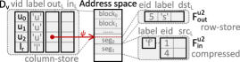
Figure 4. Memory layout and physical design

Unified address space and pointers. Following the conventional design for $\mathsf{RDBMS}$ (Özsu and Valduriez, 2020; Kemper and Neumann, 2011; Traiger, 1982) and operating systems (Silberschatz et al., 2018; Stonebraker and Kumar, 1986), a unified virtual address space is utilized for both the conventional and the extended relations. Each pointer can then be represented with a fixed length field in the following two ways. (1) The pointers can directly record the starting address of a fragment, in the unified space. (2) Alternatively, an indirect pointer is supported in conjunction with the segment-based management for segments, which records only the segment id and an offset inside the segment, along the same lines as (Piquer, 1991). The address of the fragment can then be identified by first lookup the base address of the segment via its id in a segment table and then plus with recorded offset. Such an indirect implementation simplifies the processing of graph updates (Section 4.3).

Remark. Observe the following. (1) In addition to a better memory locality, the unified virtual address space unifies the in-memory and on-disk graph data representation, and hence, makes it possible to incorporate disk-based e.g., (Fan et al., 2022c), and even distributed e.g., (Bouhenni et al., 2021) graph processing (2) Since the $\mathsf{RG}$ model is a mild extension of the relational model, most of existing physical design techniques for $\mathsf{RDBMS}$, e.g., (Athanassoulis et al., 2019; Arulraj et al., 2016; Stonebraker et al., 2005; Alagiannis et al., 2014; Rasin and Zdonik, 2013; Lightstone et al., 2007), can be leveraged as showcased in Figure 4. For instance, column-store (Stonebraker et al., 2005) can be adopted to maintain vertex and edge attribute relations to speed up the scanning of each specified column. Moreover, since the power-law degree distribution of real-life graphs (Clauset et al., 2009) often yields a number of edges that share the same label and are adjacent to the same vertex, column-oriented compression methods (Abadi et al., 2006; Lang et al., 2016) can also be adopted for storage and execution optimization.

4.3. Updating and Browsing Graphs

The logical conversion process from graph to the $\mathsf{RG}$ model shown in Section 4.1 can be reversed and incrementalized for users to browse and update graph respectively, regardless of how fragments and pointers are physically implemented to not break the physical data independence (Stonebraker, 1975).

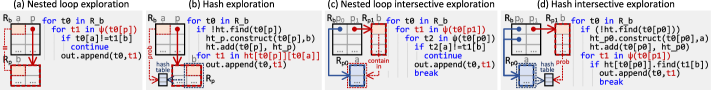
Figure 5. A demonstration of the operators introduced in the $\mathsf{RG}$ model

Browsing graphs. The graphs stored in extended relations can be browsed with explicit topology, as depicted in Figure 2, by simply reversing the graph conversion process to restore the topological structure of the graphs, in which pointers are used to fetch relevant data. Users may opt to pick entities of their interests, for the browsing to be conducted lazily and expand localized subgraphs only upon their request. Moreover, common labels and attributes of entities (vertices) and relationships (edges) can also be extracted from its extended relations, by referencing the $\mathsf{RG}$ schema for a graph $G$. It can then facilitate the creation of an ontology (Matthews, 2005) for such entities and links, such that users can easily write pattern queries over $G$.

Incremental maintenance. Real-life graphs are often updated. Consider batch updates $\Delta G=(\Delta V,\Delta E)$ to a graph $G$, which consist of a set $\Delta V$ of vertex insertions and deletions, and a set $\Delta E$ of edge insertions and deletions. Updates to vertex (resp. edge) attributes can be simulated by a sequences of vertex (resp. edge) deletions and insertions, which first delete the old vertices (resp. edges), followed by inserting the new ones with updated attributes.

Given the batch updates $\Delta G$, $\mathcal{D}_{G}^{E}$ can be maintained by (a) appending newly inserted vertices to $D_{\mathsf{V}}$ along the same lines as in the graph conversion process in Section 4.1; (b) allocating new vertex and edge attribute values to $D_{\mathsf{V_{A}}}^{l_{i}}$ and $D_{\mathsf{E_{A}}}^{l_{j}}$; (c) sorting the new edges by source vertices $v_{i}$ and destination vertices $v_{j}$, and appending them to fragments $F_{\mathsf{out}}^{v_{i}}$ and $F_{\mathsf{in}}^{v_{j}}$ accordingly; (d) identifying and removing the data about the deleted vertices and edges based on the value and reference function; and (e) revising the reference function accordingly, as described in Section 4.1.

Implementation. We implement the procedure based on the physical design of Section 4.2 as follows. Since the small fragments are stored as segments in a continuous memory space (Section 4.2), the reallocation will be conducted when the inserted tuples make the fragments exceed the capacity of their underlying segments. In particular, if the size of an enlarged fragment reaches the threshold, a block will be allocated for the block-based management to be applied on it thence, which makes the reallocation cost under control (see (ful, 2023) for an evaluation). Once a segment has been reallocated, the direct pointers point to it will need to be reassigned to tract it while the indirect pointers need not to be updated and save such a cost.

5. Hybrid Query Evaluation

In this section, we present the entire $\mathsf{RG}$-based hybrid query evaluation workflow. We first introduce the new exploration operator induced by the $\mathsf{RG}$ model that facilitates the pattern matching (Section 5.1). We then review the general strategy of query optimization in $\mathsf{RDBMS}$ (Section 5.2) and show how to extend it by incorporating exploration to evaluate hybrid queries (Section 5.3).

5.1. Exploration Operator

Based on the pointers introduced in the $\mathsf{RG}$ model, we define the exploration operator, which can be used to “explore” the data in extended relations through those pointers.

Exploration. The exploration operator, denoted as $\vec{\bowtie}^{A}_{\theta}$, is applied on an extended relation $S_{1}$, regarding one of its field $A$ as pointers, toward another extended relation $S_{2}$. Here $\theta$ is condition set that can be empty. That is, $S_{1}\vec{\bowtie}^{A}_{\theta}S_{2}$ joins every tuple $t\in S_{1}$ with each one of the tuples $t^{\prime}\in\psi(t[A])\subseteq S_{2}$ together only if $t$ and $t^{\prime}$ satisfy condition $\theta$, e.g., comparison among multiple attributes on $t$ and $t^{\prime}$.

Intuitively, if a graph $G$ is stored with the $\mathsf{RG}$ model as in Section 4, then the exploration operation is indeed analogous to exploring $G$ by, e.g., iterating over all adjacent edges of each vertex in $G$, a common step in graph algorithms, instead of a single tuple (Shekita and Carey, 1990).

Explorative condition. Besides simply verifying it over plain values, the data linked by the pointers can also be inspected in the join condition here. Considering a condition $\theta^{I}$ defined as $\psi(A)[B]\ni C$. For each tuple $t\in S_{1}$ and $t^{\prime}\in S_{2}$, $S_{1}\>{\bowtie}_{\theta^{I}}S_{2}$ checks whether there exists a tuple $t^{\prime\prime}\in\psi(t[A])$ such that $t^{\prime\prime}[B]$ matches the value of $t^{\prime}[C]$; if so, $t$ and $t^{\prime}$ are joined and returned in the result relation. As the evaluation process of such a condition will also explore the tuples pointed by $t[A]$, we refer to $\theta^{I}$ as an explorative condition.

By incorporating such a condition into an exploration operator, $S_{1}\>\vec{\bowtie}^{A}_{\theta^{I}}S_{2}$ can then pairwisely check the tuples linked by pointers in different fields, i.e., $A$ and $A^{\prime}$ of the same tuple $t\in S_{1}$ when enforcing $\theta^{I}$, just like computing the intersection of $B$-values and $C$-values w.r.t. those linked tuples. Hence we refer to $S_{1}\>\vec{\bowtie}^{A}_{\theta^{I}}S_{2}$ as the intersective exploration.

In fact, the intersective exploration can serve as a basic component, checking whether the matches of two connected pattern edges intersect at a same vertex in the data graph, i.e., an essential step in matching cyclic patterns. As will be seen shortly, the (intersective) exploration can be executed seamlessly along with other conventional operators in a pipelined manner (Boncz et al., 2005) without performance degradation. The comparison to the native graph-based pattern matching algorithms in Section 5.3 will further show how most of their strategies can then be achieved equivalently.

Example 1.

A possible logical plan to match pattern $P$ in Figure 1 on graph stored as $\mathcal{D}_{G}^{E}$, omit label checking, can be described as:

$(((D_{V}^{2}{\vec{\bowtie}^{out_{L}}}D_{o}^{1}){\vec{\bowtie}^{dst_{L}}}D_{V}^{1}){\vec{\bowtie}^{out_{L}}}_{\psi(D_{V}^{2}.in_{L})[src_{L}]\ni dst_{L}}D_{o}^{2}){\vec{\bowtie}^{dst_{L}}}D_{V}^{0}$

It represents matching the pattern with the order: $v_{2}$, $v_{1}$, $v_{0}$, where $D_{V}^{0}$, $D_{V}^{1}$ and $D_{V}^{2}$ (resp. $D_{o}^{1}$, $D_{o}^{2}$) are all aliases of $D_{V}$ (resp. $D_{out}$).

Physical implementations. Same as the standard operators supported by $\mathsf{RDBMS}$, each logical exploration operator can also correspond to multiple physical operators in different scenarios. We first use a logical exploration: $R_{b}{\vec{\bowtie}^{p}}_{a=b}R_{p}$, where field $R_{b}[p]$ consists of pointers toward fragments, as an example to show how various physical operators can correspond to it, and then consider the explorative condition.

Nested-loop exploration. As the most native implementation, once a tuple $t_{0}\in R_{b}$ has been enumerated, $t_{0}[p]$ will be dereferenced to locate the fragment it points to. Thence all tuples $t_{1}\in\psi(t_{0}[p])$ can then be accessed and iterated in a nested loop manner to directly verify equalities as shown in Figure 5(a). The $t_{0},t_{1}$ pairs can then be exported if there are $t_{0}[a]\text{=}t_{1}[b]$. Such an implementation will be very efficient if all $t_{0}[p]$ point to relatively small fragments.

Hash exploration. Alternatively, the hash-based methods can also be considered to speed up the equality checking by constructing a hash table for the data to be probed. That is, as shown in Figure 5(b), a large hash table $ht$ will be maintained. For each enumerated tuple $t_{0}\in R_{b}$, it will be first checked whether there already exists a hash table $ht_{p}$ in $ht$ corresponding to the value in $t_{0}[p]$. If not, such a $ht_{p}$ will be constructed, to hold all tuples $t_{1}\in\psi(t_{0}[p])$ and the value of their field $t_{1}[b]$, and be stored in $ht$ corresponding to $t_{0}[p]$; otherwise, such a pre-constructed $ht_{p}$ can be directly reused to find all tuples $t_{1}\in\psi(t_{0}[p])$ s.t. $t_{0}[a]\text{=}t_{1}[b]$.

Note that those hash tables stored in $ht$ can be reused for different tuples in $R_{b}$ that have the same value in their pointer field, and thus eliminate the need of duplicate construction. A performance improvement can then be achieved if the pointers in column $R_{b}[p]$ all point to relatively large fragments and a large portion of them have the same value, i.e., toward the same set of tuples. This can happen when $R_{b}$ is the intermediate result of the pattern matching where the same vertex from data graph can appear multiple times in different partial matches. Other typical physical implementations for the join operator, e.g., index, merge sort etc. (Lightstone et al., 2007), can also be considered for exploration but will not be further discussed here.

Explorative condition. As the explorative condition cannot be simply evaluated by verifying the plain value of the two input tuples, we consider a logical intersective exploration: $R_{b}{\vec{\bowtie}^{p_{1}}}_{\psi(p_{0})[a]\ni b}R_{p_{1}}$, and demonstrate the nested loop and hash-based physical operators corresponding to it in Figure 5(c) and 5(d) respectively.

5.2. Relational Query Optimization Overview

We then show how only a few minor extensions, without modifying the overall and the various sophisticated detailed technologies, will be required for the conventional $\mathsf{RDBMS}$ to take the exploration into consideration to facilitate the evaluation of both pattern query and hybrid query. Before showing the extensions required in each step, the hypergraph-based conventional relational query optimization workflow (Abiteboul et al., 1995; Chaudhuri, 1998) will first be reviewed here.

Generally speaking, in a conventional $\mathsf{RDBMS}$ optimizer, the input $\mathsf{SQL}$ query will first be parsed to generate an unoptimized logical query plan in a canonical form (Hellerstein et al., 2007) accordingly. After that, a query graph (Bernstein and Chiu, 1981) will be constructed correspondingly where each relation (resp. constant) in the input logical plan will be modelled as a node and each join or selection condition will be represented as an edge. Each edge connects multiple nodes for relation or constant involved in the corresponding condition (Abiteboul et al., 1995), making those edges hyperedges and the query graph a hypergraph.

Such a hypergraph equivalently represents the input declarative query while providing an elegant perspective for it to become the input of most query optimization algorithms especially for join reordering (Fender and Moerkotte, 2013; Bhargava et al., 1995; Moerkotte and Neumann, 2008). Each CSG (Connected SubGraph) in the query graph denotes a possible subquery, and each partition of a CSG into a CMP (connected complement) pair, regarding all edges that connect them as join conditions, can then be resolved as a join operator. That is, by enumerating all possible top-down partitions from the entire query graph down to the CSGs with only one node, all possible join orders can then be considered. Heuristic methods (Steinbrunn et al., 1997; Neumann, 2009) or several restrictions on the join tree topology (Ahmed et al., 2014), e.g., to be left-deep (Ioannidis and Kang, 1991), can be utilized in such an enumeration process as a trade-off to reduce the plan space.

The cost of each enumerated join tree will then be evaluated for the optimal query plan among them to be selected accordingly. The cardinality of each CSG in the join tree will first be estimated (Leis et al., 2017; Heule et al., 2013; Lu and Guan, 2009; Poosala et al., 1996; Lipton et al., 1990; Müller et al., 2018; Perron et al., 2019), and a cost model (Manegold et al., 2002a; Bellatreche et al., 2013; P.G. et al., 1979) will be further utilized to consider the physical execution process, to generate an optimal physical plan for final execution. If the pipelined execution (Boncz et al., 2005) is utilized, the generated physical query plan will be further divided into pipelines according to the operators that can break the pipeline execution.

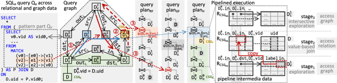
Figure 6. A demonstration of the hybrid query evaluation process with the $\mathsf{RG}$ model

Extension. It will be shown that the above workflow only needs to be extended at three minor points to incorporate the exploration and the $\delta$-join to support the graph pattern and hybrid query:

(1) Exploration representation. We introduce a new kind of exploration edge into the query graph. Using this revised query graph as the input, the existing optimization strategies can then be directly applied on it to support hybrid query with slight revises.

(2) Exploration cost estimation. We extend the cost estimation methods for conventional relational query to consider the query plan that contains the exploration operator.

(3) Dynamic entity resolution. The $\delta$-join will be introduced as an operator for dynamic entity resolution according to the query from the user, which will not increase difficulty compared to existing relational operators.

Those modifications are all minor without the need to touch the well-developed sophisticated optimization techniques from plan enumeration to cost estimation.

5.3. Hybrid Query Optimization

We now present the extensions on the query optimization workflow enabled by the $\mathsf{RG}$ model, which are all minor and allow most of the well-developed sophisticated optimization techniques to be directly inherited. The hybrid query can then be optimized in an enlarged unified space and evaluated without performance degradation.

Optimization workflow with exploration. We first show how the conventional query graph can be extended to uniformly represent the hybrid query, followed by the modifications required on the existing optimization methods for them to be applied on such an extended query graph.

Exploration representation. We introduce exploration edge to represent the exploration through pointers in the query graph along with the hyperedges for join and select conditions. An exploration edge has the form $(S_{1},A,S_{2})$ that directly links the extended relation $S_{1}$ to $S_{2}$ and is labelled by the field of the pointer to be explored, which can be resolved into an exploration operator: $S_{1}{\vec{\bowtie}^{A}}S_{2}$. The hybrid query can then be encoded with such a query graph uniformly to provide an enlarged unified plan space for optimization.

We then show how the pattern part $Q_{P}$ of an input ${\mathsf{SQL_{\delta}}}$ query can be encoded with such a query graph, while the rest part can still be constructed as it used to be. To simplify the description below, we skip the trivial parsing step for generating the canonical logical plan and directly show how the extended query graph can be constructed corresponding to $Q_{P}$. Assume the data graph is stored in the extended relations $\mathcal{D}_{G}^{E}$ as described in Section 4, for each pattern vertex $v_{i}$ in $Q_{P}$, we add a node $D_{\mathsf{V}}^{i}$ into the query graph as an alias of the extended relation $D_{\mathsf{V}}$. A pulled down filter condition for vertex label checking, i.e., to be $L_{P}(v_{i})$, will then be contained in such a node in the query graph and associated with its field “label”.

For each edge $e_{i}=(v_{j},v_{k})$ in $Q_{P}$, two nodes $D_{\mathsf{out}}^{i}$ and $D_{\mathsf{in}}^{i}$, alias of $D_{\mathsf{out}}$ and $D_{\mathsf{in}}$ respectively, will be included into the query graph and also be associated with a filter condition to check the “label” to be $L_{P}(e_{i})$. After that, four exploration edges $(D_{\mathsf{V}}^{j},\mathsf{out_{L}},D_{\mathsf{out}}^{i})$, $(D_{\mathsf{out}}^{i},\mathsf{dst_{L}},D_{\mathsf{V}}^{k})$, $(D_{\mathsf{V}}^{k},\mathsf{in_{L}},D_{\mathsf{in}}^{i})$ and $(D_{\mathsf{in}}^{i},\mathsf{src_{L}},D_{\mathsf{V}}^{j})$ will be incorporated into the query graph, which form two opposite paths and enable two alternative exploration directions induced w.r.t. the same pattern edge $e_{i}$. Such a redundancy introduced on purpose enlarges the optimization space for enumerating query plans. Finally, “same-pointer conditions” will be generated among different exploration edges toward the same node in the query graph, directly comparing the value of the pointer to restrict them to point to the same tuple. It then allows the explorative condition to be resolved during the query plan generation (see below), and helps to compute the intersection of matched vertices, an essential step to optimize matching the cyclic patterns. (see (ful, 2023) for a formal definition of query graph).

Example 2.

Figure 6 shows the query graph corresponding to an example ${\mathsf{SQL_{\delta}}}$ query simplified from the one in Example 2, where the labels of both vertices and edges in its pattern part $Q_{P}$ are all omitted. Taking edge $e_{1}$ as an example, it corresponds to two opposite paths with edges: $(D_{V}^{2},out_{L},D_{o}^{1})$, $(D_{o}^{1},dst_{L},D_{V}^{1})$; and $(D_{V}^{1},in_{L},D_{i}^{1})$, $(D_{i}^{1},src_{L},D_{V}^{2})$, respectively. This denotes that the edge can be explored from two directions. Meanwhile, the value-based join across relation and graph data is also represented as an edge connecting the nodes $D$ and $D_{V}^{0}$ uniformly. The same-pointer conditions, e.g., $D_{i}^{2}[src_{L}]=D_{i}^{1}[src_{L}]$, are not shown in Figure 6 as a simplification (see (ful, 2023) for a step-by-step explanation).

Hybrid query plan enumeration. The enlarged unified plan space for hybrid queries, facilitated by the extended query graph, allows the access on graph and relational data to be considered in any order. The value-based join with low selectivity can then be pulled down into the pattern matching process in the generated plan for optimization according to the estimated cost (see below).

By accepting the extended query graph as input, CSG-CMP pairs can still be exported from it using existing mainstream plan enumeration methods (Fender and Moerkotte, 2013; Moerkotte and Neumann, 2008; Steinbrunn et al., 1997; Neumann, 2009). There are only a few differences on the following steps to resolve them into exploration operators:

(1) If an enumerated CSG-CMP pair is connected by an exploration edge, then we add the exploration operator it encodes to the query plan according to the edge’s direction. The prob-side CSG, i.e., the one pointed by the exploration edge, is required to contain only one node in the query graph, to ensure the pointer will not be used to track the data that have already been moved into the intermediate result. This restriction is not tighter than that of the left-deep trees, which are frequently enforced to achieve pipelined execution in $\mathsf{RDBMS}$ (Boncz et al., 2005), and one can easily verify that such a legal query plan always exists.

(2) A node in the extended query graph can be resolved as an explorative condition incorporated into other operators. That is, once a CSG-CMP pair, $CSG_{0}$ and $CSG_{1}$, is enumerated, an operator $op_{i}$ will be resolved according to the edges that directly connect them. After that, it will be checked whether there exist another node $n_{i}$ in the query graph, such that: (a) there exists an exploration edge from a node in $CSG_{0}$ (resp. $CSG_{1}$) toward $n_{i}$, and (b) there exists an edge for plain-value join connects $n_{i}$ and a node in $CSG_{1}$ (resp. $CSG_{0}$). For each node $n_{i}$ that satisfies these two requirements, it will be resolved as an explorative condition and be incorporated into $op_{i}$, which does not need to be further contained in other CSGs.

(3) The nodes that are duplicated to each other in the query graph will not be both contained in the generated query plan. That is, when enumerating the query plan, it will be guaranteed that only one path among each duplicate path pairs in the query graph is inspected w.r.t. the corresponding pattern edge. Hence, the space for planning is enlarged without introducing duplicated computation into the generated query plan (see (ful, 2023) for an overall description).

Exploration cost estimation. We also present a method for estimating the cost of query plans w.r.t. hybrid queries, for the optimal plan to be selected from all those enumerated accordingly. Here we opt to extend the previous cost estimation strategies for $\mathsf{RDBMS}$, which are based on (1) cardinality estimation, and (2) a cost model to evaluate each operator in the query plan.

To estimate the cardinality of intermediate results, we inherit the existing estimation approaches that are designed w.r.t. either the general relational queries in $\mathsf{RDBMS}$ e.g., (Leis et al., 2017; Perron et al., 2019), or the specific pattern matching task e.g., (Park et al., 2020; Kim et al., 2021), and even using some AI-based methods (Zhou et al., 2022). This is inspired by the fact that the same number of matched results will be deduced when matching a given pattern on the data graph, no matter how the data is modelled.

Since all operators in the conventional relational query plan remain intact in the query plan for hybrid queries, we bring a slight revision of the existing cost models for $\mathsf{RDBMS}$ to consider the introduced operators, instead of developing a new one from scratch. As an example, below we show that the simple cost function $C_{mm}$ (Leis et al., 2015), which is tailored for the main-memory setting, can be extended to an other model, denoted as $C_{emm}$, as follows.

$$C_{emm}(T)=\begin{cases}C_{emm}(T_{1})+\tau|T_{1}[A]|\quad\text{(if $T=T_{1}\vec{\bowtie}^{A}_{\theta}T_{2}$, nested loop)}\\ C_{emm}(T_{1})+\tau|\Pi_{A}(T_{1})[A]|+|T|\ \ \text{(if $T=T_{1}\vec{\bowtie}^{A}_{\theta}T_{2}$, hash)}\\ \@@ams@intertext{$C_{emm}(T_{1})+\tau|T_{1}[A]|\times\frac{1}{2}|T_{1}[A^{\prime}]|/|T_{1}|$}\cr\vspace{-2.5ex}\@@ams@intertext{\qquad\qquad\qquad\text{(if $T=T_{1}{\vec{\bowtie}^{A}}_{\psi(A^{\prime})[a]\ni b}T_{2}$, nested loop)}}\cr\vspace{-2.5ex}\@@ams@intertext{$C_{emm}(T_{1})+\tau|T_{1}[A]|+\tau|\Pi_{A^{\prime}}(T_{1})[A^{\prime}]|+|T|$}\cr\vspace{-2.5ex}\@@ams@intertext{\qquad\qquad\qquad\text{(if $T=T_{1}{\vec{\bowtie}^{A}}_{\psi(A^{\prime})[a]\ni b}T_{2}$, hash)}}\cr\end{cases}$$

Here only the estimated cost for the physical (intersective) exploration operator is shown, i.e., using nested loop or hash table; $|S|$ (resp. $|S[A]|$) denotes the cardinality estimated for relation $S$ (resp. data linked by the pointer in the field $A$ of all tuples in $S$); and $\tau\leq 1$ represents the cost of table scan compared to join (Leis et al., 2015). Intuitively, the nested-loop methods will iterate over all tuples pointed by the pointer; while the hash-based methods allow the pointer with same value to be reused and thus only need to consider the cardinality after projection. The cost for other conventional relational operators follows from the counterparts in (Leis et al., 2015); while the cost for $\delta$-join is estimated by the complexity of the ER method applied.

The following example provides an overall demonstration of how various hybrid query plans that access graph and relational data in different orders can be enumerated and then executed without performance degradation:

Example 3.

Figure 6 shows three representative query plans corresponding to the ${\mathsf{SQL_{\delta}}}$ query $Q_{\delta}$: $\text{Plan}_{\text{RF}}$, $\text{Plan}_{\text{GF}}$, and $\text{Plan}_{\text{H}}$, that access the relational data at first, at last and during the pattern matching process respectively. $\text{Plan}_{\text{H}}$ is highlighted as a typical example to show how a hybrid query plan can be generated through CSG-CMP pair enumeration and then be executed with a seamlessly access on graph and relational data without switching to another relational/native graph-based engine (see (ful, 2023) for details).

Intuitively, if the join on $D$ and $D_{V}^{0}$ in Figure 6 has a low selectivity but is not lower than the partial match of vertices $v_{0}$ and $v_{1}$, $\text{Plan}_{\text{H}}$ will then have the lowest cost among the three of them. The experimental results in Section 6 show that optimizing the hybrid query in such an enlarged unified plan space and pulling the join conditions down to the pattern matching process in such a way can bring a $10.1\times$ speedup on average.

Dynamic entity resolution with $\delta$-join. As the ER algorithm is regarded as a black box here, each $\delta$-join $Q_{1}\bowtie_{\delta}Q_{2}$ will be constructed as a hyperedge in the query graph that links to all nodes involved in subqueries $Q_{1}$ and $Q_{2}$, along the same lines of handling the union and set difference operators. As for the query plan generation, optimized plans for its subqueries will first be generated separately and the result relation of the $\delta$-join will be treated as a base relation for applying global optimizations further, in a way similar to that for aggregation operators in conventional relational query plans (Galindo-Legaria and Joshi, 2001) without bringing more difficulty.

During the execution process, the ER algorithm will be conducted once all results of its subqueries have been obtained. Such an operator will also be able to move across the plan tree and the required space for intermediate result can thence be reduced if it can be assumed that the utilized ER algorithm will always join or not join two tuples independently instead of being treated as a black box. We defer the study on this to future work.

Comparison to native graph-based algorithms. The introduced exploration operator provides the most fundamental component in the native graph-based algorithms, while the revised $\mathsf{RDBMS}$ optimizer can equivalently perform the matching order selection. Moreover, the capability for hybrid query also allows the candidate sets to be integrated for optimization which are widely adopted in the state-of-the-art pattern matching algorithms (Sun and Luo, 2020a). That is, candidate set $C(v_{i})$ can be generated for each pattern vertex $v_{i}$ using any of existing methods and stored in a separated relation $D^{C}_{v_{i}}$ with one column $vid$ only for the vertex id. The generated candidate set can then be used for vertex filtering as a join: $D^{C}_{v_{i}}\bowtie_{vid=vid}D_{\mathsf{V}}^{i}$.

The query-related data-driven declarative optimization workflow actually allows the candidate sets to be better utilized, where only the ones that can bring more benefits than cost will be considered instead of all of them. That is, as those additional joins on the candidate sets will not differ the query result, if the join tree with the lowest cost does not contain all these joins on the candidate set, it can still be confidently selected to generate the query plan. It can thus avoid considering the candidate set with high selectivity, i.e., cannot prune many vertices, for performance improvement.

Remark. By considering the exploration as an operator, most of the other native graph-based pattern matching optimizations can also find their $\mathsf{RDBMS}$ alternatives. As an example, sideway information passing (Neumann and Weikum, 2009) holds a similar idea as the failing set (Han et al., 2019); The adaptive execution (Deshpande et al., 2007), well-studied in the database community, can somewhat be regarded as a more advanced adaptive query ordering (Han et al., 2019; Han et al., 2013). Meanwhile, optimizations from the database community on query execution (Boncz et al., 2005; Menon et al., 2017; Neumann, 2011; Li and Patel, 2013; Zhou and Ross, 2002; Schuh et al., 2016), a stage that is rarely studied in the research of graph pattern matching algorithms (Yang et al., 2021; Bhattarai et al., 2019; Han et al., 2019; Huang et al., 2014; Cordella et al., 2004) whose workflow essentially coincide with the volcano model (Graefe and McKenna, 1993), can also bring advantages to exceed them.

6. System and evaluation

We carry out $\mathsf{WhiteDB}$, an implementation of the proposed $\mathsf{RG}$ model, to evaluate the benefits it can bring on real-world data.

6.1. System Implementation

We implemented the entire $\mathsf{WhiteDB}$ extended from DuckDB (Raasveldt and Mühleisen, 2019). We introduced the exploration operator and the exploration condition into both the logical and physical plans as in Section 5.1, and then integrated them into the query optimization workflow as in Section 5.3. We added a filter atop of the plan enumeration method (Moerkotte and Neumann, 2008) adopted in DuckDB to resolve exploration operator from CSG-CMP pairs enumerated from the extended query graph as described in Section 5.3 (see (ful, 2023) for the details). We used a simple histogram to estimate the “selectivity” of the exploration in the optimizer, and the experiment results show it works sufficiently well.

For physical plan generation, we utilized a simple heuristic approach which will generate hash (intersective) exploration operator only if the base-side relation is a pipeline intermediate result and the explored pointers are not point to single tuple; the nested-loop (intersective) exploration will be considered otherwise. We integrated the introduced operators into the pipelined execution engine (Boncz et al., 2005) as shown in Figure 6 with the size of the pipeline intermediate result set to $2048$ as in DuckDB (Raasveldt and Muehleisen, [n.d.]). For all extended relations, we uniformly considered the row-store as the physical implementation. Meanwhile, we opted to divide the first input relation of the pipeline into several subsets and duplicate the pipeline into multiple copies to process them in parallel to support intra-query parallelism.

For entity resolution, we integrated JedAI (Papadakis et al., 2018), one of the most advanced open-sourced ER implementation we can find, using their official implementation with Java and called it from the C++-side through the JNI (Java Native Interface) (Gabrilovich and Finkelstein, 2001) for dynamic entity resolution. We used group linkage in the entity matching step and unique mapping clustering in the entity clustering step according to its characteristics following (Papadakis et al., 2020). $\mathsf{WhiteDB}$ also provides a native graph interface to support imperative programming as shown in Figure 2. Based on it, we implemented the candidate set generation method in (Han et al., 2019) to optimize the pattern-part of ${\mathsf{SQL_{\delta}}}$ query as in Section 5.3.

6.2. Experimental Study

Using real-life datasets, we empirically evaluated $\mathsf{WhiteDB}$ for its (a) efficiency, (b) scalability and (c) effectiveness in enrichment.

Experimental setting. We start with the experimental settings.

Datasets. We used three real-life graphs: (1) $\mathsf{DBLP}$ (Schloss Dagstuhl, [n.d.]), a real-life citation network with $0.2$M vertices and $0.3$M edges, constituting bibliographic records of research papers in computer science; (2) $\mathsf{YAGO}$ (Mahdisoltani et al., 2013), a knowledge graph with $3.5$M vertices and $7.4$M edges; (3) $\mathsf{IMDB}$ (imd, 2023), a graph database that includes attributes for the information of movies, directors and actors, having $5.1$M vertices and $5.2$M edges. (4) $\mathsf{movieLens}$ (mov, 2021), a rating network with $25$M of 0.0~5.0 rating from $0.16$M users to $59$K movies, each user vertex holds a unique $uid$ and each movie vertex holds its $title$ and $genres$. And two real-life relations: (1) $\mathsf{DBpedia}$ relations (dbp, 2023a), where the $\mathsf{Celebrity}$ (dbp, 2023d, e) intersects with the peoples in $\mathsf{YAGO}$ and the $\mathsf{Journal}$ (dbp, 2023c) intersects with the journals in $\mathsf{DBLP}$; (2) The structuralized nationality of movies from $\mathsf{LinkedMDB}$ (Hassanzadeh and Consens, 2009), that intersects with the movies in $\mathsf{IMDB}$.

Baselines. We considered four types of baselines to evaluate the performance of $\mathsf{WhiteDB}$: (1) Relational systems, we utilized PostgreSQL (v13.5) (Stonebraker et al., 1990) and DuckDB (Raasveldt and Mühleisen, 2019); (2) Native graph-based systems, we utilized Neo4J (v5.6.0) (neo, 2023) and GraphFlow (Kankanamge et al., 2017); (3) Native graph-based algorithms, we utilized CECI (Bhattarai et al., 2019), DP-iso (Han et al., 2019), TurboFlux (Kim et al., 2018), IEDyn (Idris et al., 2017) and SymBi (Min et al., 2021). Following the recommendation in (Sun and Luo, 2020b), we also combined the candidate vertex computation method of GraphQL (He and Singh, 2009) with the ordering methods and auxiliary data structures of DP-iso as another baseline, denoted as GQL-DPiso; (4) Relational system with pattern matching-oriented optimization, we utilized GRainDB (Jin and Salihoglu, 2022) which is not merely acting as an interface atop of $\mathsf{RDBMS}$ for query mapping.

For DuckDB, we used their official open-source C++ implementation (Raasveldt and Muehleisen, [n.d.]). The rest baselines, GraphFlow, CECI, DP-iso, GQL-DPiso, TurboFlux, IEDyn and SymBi, we directly utilized the C++ implementations in (Sun et al., 2022; Sun and Luo, 2020b) as a fair comparison.

Configuration. The $\mathsf{WhiteDB}$ and other baselines implemented in C++ are all compiled with GCC-12 and are set to use single thread if not specially mentioned. The experiments were run on a desktop with 3.2GHz processor and 16 GB memory.

Experimental results. We next report our findings.

Exp-1: Case study. We first validated the need to enrich relational data (resp. graph) with graph properties (resp. relational data) all in $\mathsf{RDBMS}$. Considering movie recommendation over datasets: (1) Graph data $\mathsf{movieLens}$, denoted as $G_{M}$. (2) User portrait $D_{U}(uid,genre_{0},\dots,genre_{2})$ of their top three interesting genres. Its field $uid$ aligns with the $uid$ of user vertices in $G_{M}$ and is not merely an equivalent relational representation of $G_{M}$. (3) $D_{M}(title,country)$ from $\mathsf{LinkedMDB}$ of the title and country of each movie, the value of title here cannot directly match with the $title$ property of movie vertex in $G_{M}$, as they can be stored in different forms and errors often occur.

As shown in Figure 7, $\mathsf{WhiteDB}$ can recommend movie $m_{0}$ to user $u_{1}$ according to: (1) $u_{0}$ (resp. $u_{1}$) rates $m_{0}$, $m_{1}$ and $m_{2}$ (resp. $m_{1}$ and $m_{2}$) as $5.0$; (2) $m_{0}$, $m_{1}$ and $m_{2}$ all from the same country, according to the data enhanced from $D_{M}$; (3) $m_{0}$ is marked with two genres, Drama and Romance, two of the $u_{1}$ favourites according to the portrait of it from $D_{U}$. This task cannot be fairly achieved by: (1) Various data enrichment or graph data extraction methods, they are not developed to extract data from graph strictly according to the pattern specified by users; (2) $\mathsf{RDBMS}$ or other relation-based polyglot systems, as their performance does not allow them to query graph data with such a complicated pattern (¿10hr in DuckDB); (3) Native graph-based systems, the result of graph query (¿$10^{10}$ matches) needs to be exported into the $\mathsf{RDBMS}$ for further relational processing with the data in it; (4) Static offline entity resolution, since both $D_{M}$ and $G_{M}$ are updated frequently, which can invalidate the precomputed result; (5) Combinations of the above methods, which fail to optimize the hybrid query in a unified space, not even to mention the cost of data movement and format conversion.

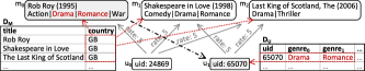
Figure 7. A case study on the movie recommendation task

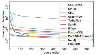
(a) $\mathsf{DBLP}$: Pattern matching speedup

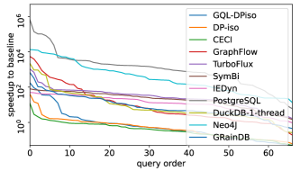
(b) $\mathsf{IMDB}$: Pattern matching speedup

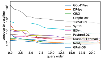
(c) $\mathsf{YAGO}$: Pattern matching speedup

Figure 8. Pattern query performance evaluation

Exp-2: Pattern query efficiency. The most significant difference for $\mathsf{WhiteDB}$ to depart from previous relational systems is the efficiency on pattern queries by utilizing the more efficient operators induced by the $\mathsf{RG}$ model. We first evaluated the performance of $\mathsf{WhiteDB}$ on pattern queries compared to various baselines, to prove that it can bring orders of magnitude speedup compared to other relational systems and is also comparable to the most efficient native graph-based pattern matching algorithms. The patterns used here are all discovered from their underlying data graphs as in (Fan et al., 2022a).

Comparison to all baselines. We first carried out an experiment to compare $\mathsf{WhiteDB}$ to all kinds of baselines we considered, to evaluate the efficiency on pattern query. Restricted by the performance of some baselines, especially the relational ones, we only used a small number of simple patterns here: 761 (8 cyclic), 68 (0 cyclic) and 23 (1 cyclic) patterns on $\mathsf{DBLP}$, $\mathsf{IMDB}$ and $\mathsf{YAGO}$ respectively. Figures 8(a) to 8(c), show the speedup $\mathsf{WhiteDB}$ brings compared to all baselines on all these patterns, ordered in a descending order.

The experimental results show that $\mathsf{WhiteDB}$ is orders of magnitude more efficient than the relational baselines: 32500x to PostgreSQL and 112x to DuckDB with one thread (121x when both used 4-threads). Meanwhile, the enormous size of intermediate result, ¿$100GB$ in some cases, required by these relational baselines much beyond the typically capability of main-memory, which brought an unaffordable cost for them to be written on disk and thence forbidden a large portion of queries here to be executed. $\mathsf{WhiteDB}$ also achieved a 34.0x speedup compared to GRainDB, as it only optimizes pattern query with sideway-information-passing. Although such a relatively less aggressive way optimization allows it to achieve a visible performance improvement compared to DuckDB, it still fails to compare with the most efficient algorithms.

$\mathsf{WhiteDB}$ achieved an efficiency improvement compared to the native graph-based systems, 1640x to Neo4J and 106x to GraphFlow. It should be admitted that a large portion of the speedup compared to Neo4J actually came from the efficiency improvement our C++-based implementation brought compared to their Java-based one. However, for GraphFlow, although the C++-based implementation we utilized (Sun et al., 2022) eliminates such a gap, it still fails to consider the pipelined execution and utilize any of the candidate set selection methods.

$\mathsf{WhiteDB}$ achieved an efficiency improvement compared to several native graph-based algorithms: 36.7x to TurboFlux, 40.9x to IEDyn and 20.9x to SymBi. As only a limited number of simple patterns were used here, it can only be roughly seen that $\mathsf{WhiteDB}$ has a similar performance compared to the most efficient baselines, i.e., GQL-DPiso, DP-iso and CECI, which will be compared in details in the following experiments with a larger number of patterns.

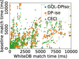
(a) $\mathsf{DBLP}$

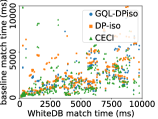
(b) $\mathsf{IMDB}$

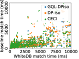
(c) $\mathsf{YAGO}$

Figure 9. Pattern matching time of $\mathsf{WhiteDB}$ and baselines

Comparison to the most efficient baselines. After proving that the implemented $\mathsf{WhiteDB}$ can bring orders of magnitude improvement compared to other baselines, we used a large amount of patterns to empirically evaluate its efficiency compared to the most efficient baselines: 3333 (1908 cyclic), 417 (257 cyclic) and 2485 (1445 cyclic) patterns on $\mathsf{DBLP}$, $\mathsf{IMDB}$ and $\mathsf{YAGO}$ respectively. Figures 9(a) to 9(c) visually present the performance of $\mathsf{WhiteDB}$ and the baselines on these patterns, where the X-axis (resp. Y-axis) represents the execution time on $\mathsf{WhiteDB}$ (resp. baseline).

Generally speaking, the experimental results prove that the $\mathsf{RG}$ supports $\mathsf{WhiteDB}$ to achieve a comparable performance compared to these most efficient native graph-based pattern matching algorithms: 1.01x to GQL-DPiso, 1.20x to DP-iso and 1.41x to CECI, which is even less significant than the variation among different native graph-based algorithms. In particular, $\mathsf{WhiteDB}$ achieved a visible speedup on a portion of queries and can be very significant in some cases, that might own to: (1) the pipelined execution method fairly deploys the locality of the graph structure and is more efficient than the tuple-by-tuple one; (2) the heuristic ordering methods miss the optimal plan. (3) uniformly considering the candidate set for all vertices in all queries lowers the performance in some cases.

$\mathsf{WhiteDB}$ failed to achieve the same performance on some patterns, which might be due to: (1) the requirement of runtime resolving the type of data and operator in $\mathsf{WhiteDB}$, as in other RDBMSs; (2) some optimizations utilized in native graph-based algorithms cannot be considered in $\mathsf{RDBMS}$ developed for general tasks, like pre-sorting the adjacent vertex id to directly utilize the merge intersection. (3) the current implementation of $\mathsf{WhiteDB}$ does not support adaptive query execution to consider different matching order in different portions of the data graph. We defer introducing adaptive query execution into $\mathsf{WhiteDB}$ to future work.

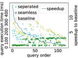
(a) $\mathsf{DBLP}$ $\times$ $\mathsf{DBpedia}$

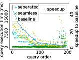
(b) $\mathsf{IMDB}$ $\times$ $\mathsf{LinkedMDB}$

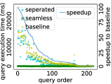
(c) $\mathsf{YAGO}$ $\times$ $\mathsf{DBpedia}$

Figure 10. Hybrid query performance

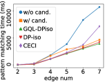
(a) $\mathsf{DBLP}$

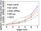
(b) $\mathsf{IMDB}$

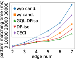
(c) $\mathsf{YAGO}$

Figure 11. Scalability of $\mathsf{WhiteDB}$

Exp-3: Hybrid query. We evaluated the performance improvement $\mathsf{WhiteDB}$ achieved on hybrid queries. For each pattern, we selected two vertices from it for them to join on the corresponding relational data, and thence resulting in 184, 254 and 207 hybrid queries on $\text{{$\mathsf{DBLP}$}}\times$$\mathsf{DBpedia}$, $\text{{$\mathsf{IMDB}$}}\times$$\mathsf{LinkedMDB}$ and $\text{{$\mathsf{YAGO}$}}\times$$\mathsf{DBpedia}$ respectively. We considered the baseline as: (1) utilize GQL-DPiso to estimate the cost of pattern-part of the ${\mathsf{SQL_{\delta}}}$ query; (2) store the entire match results into DuckDB; (3) complete the rest relational processing, and added the time they consume together. Further, we generated two kinds of query plans for hybrid query in $\mathsf{WhiteDB}$: (a) Separated, we first generated the optimized plan for the pattern part of the ${\mathsf{SQL_{\delta}}}$ query and then added additional joins on the external relations on top of it. Such a plan can be executed all inside $\mathsf{WhiteDB}$ without storing the intermediate result into another separated engine. However, it still needs to first complete the entire pattern matching process and failed to make a full use of the capability for hybrid query optimization in $\mathsf{WhiteDB}$; (b) Seamless, we further optimized the “separated” hybrid query plan within the unified enlarged plan space to pull the low selectivity joins down into the pattern matching process.

Figures 10(a) to 10(c) demonstrate their performance on those hybrid queries, sorted in a descending order of the speedup “seamless” achieved compared to the baseline. The experimental result shows that $\mathsf{WhiteDB}$ achieved a visible speedup (¿10x) on 7.38%, 39.8% and 51.4% of the queries and on average achieved 3.62x, 12.9x and 23.9x speedup on $\text{{$\mathsf{DBLP}$}}\times$$\mathsf{DBpedia}$, $\text{{$\mathsf{IMDB}$}}\times$$\mathsf{LinkedMDB}$ and $\text{{$\mathsf{YAGO}$}}\times$$\mathsf{DBpedia}$ respectively. The cost to hold the entire match result, which can easily reach billions, and store them into a separated engine largely slows down the performance of the baseline. Among the dataset we used, the speedup it achieved on $\mathsf{DBLP}$ is relatively less significant, which is due to the cost to complete the entire pattern matching is relatively cheap and the match count is also relatively small. More specifically, “seamless” also achieved 10.1x speedup compared to “separated” by pulling the low selectivity join conditions down for early pruning on average of all data graphs, which shows that optimizing hybrid query in enlarged unified plan space contributes a large portion of the speedup.

Exp-4: Scalability. We evaluated $\mathsf{WhiteDB}$ with larger patterns and showed the average execution time for the patterns with different number of edges in Figures 11(a) to 11(c), where “w/o cand.” (resp. “w/ cand.”) represents $\mathsf{WhiteDB}$ without (resp. with) considering candidate set. The result shows the performance of $\mathsf{WhiteDB}$ will not degrade and is still comparable to the baselines when the patterns scale to 7 edges, 0.91x, 1.15x and 1.68x compared to GQL-DPiso, DP-iso and CECI respectively on average of all data graphs. Moreover, the capability for $\mathsf{WhiteDB}$ to consider the candidate set brings visible improvement for large patterns, 3.17x for the patterns with 7 edges on average of all data graphs. It fairly proved that the proposed evaluation workflow is not only suitable to small patterns.

Graph	Candidate set	Hash operator	Pipeline	Optimizer
$\mathsf{DBLP}$	4.10x	4.90x	3.82x	3.79x
$\mathsf{IMDB}$	1.66x	4.25x	5.64x	11.9x
$\mathsf{YAGO}$	2.33x	5.98x	4.50x	13.3x

Table 1. Ablation study on the efficiency of pattern query

Exp-5: Ablation study. Finally, we performed an ablation study to investigate how much efficiency improvement each component contributes, with the same set of queries used in Exp-2. We omitted the four components one-by-one to evaluate the speedup they brought. As shown in Table 1, the candidate set, the hash operators, the pipelined execution and the optimizer contribute 2.70x, 5.04x, 4.65x and 9.66x efficiency improvement on average of all data graphs respectively. It can be seen that it is the advantage brought by the pipelined execution that makes up the benefits that can be brought by other optimization strategies in various native graph-based algorithms not considered here.

Summary. We find the following. (1) Modelling graph data with the $\mathsf{RG}$ model induces an exploration operator into the relational query evaluation workflow, which allows $\mathsf{WhiteDB}$ to outperform other relational systems with orders of magnitude on pattern query, 32500x to PostgreSQL and 112x to DuckDB. A comprehensive experiment with a large number of patterns also proved that it allows $\mathsf{WhiteDB}$ to achieve a comparable performance to the most efficient graph-based algorithms, 1.01x to GQL-DPiso, 1.20x to DP-iso and 1.41x to CECI. (2) By optimizing the hybrid query in an enlarged unified plan space and evaluate it without involving cross model access, $\mathsf{WhiteDB}$ achieves a 13.5x speedup. (3) $\mathsf{WhiteDB}$ still works for large patterns, 0.91x compared to the most efficient native graph baselines as the patterns scale to 7 edges.

7. Related Work

We categorize the related work as follows.

Polyglot systems. The performance on pattern query of the relation-based polyglot systems (Jindal et al., 2015; Jindal et al., 2014; Steer et al., 2017; Zhao and Yu, 2017; Zhang et al., 2022) is essentially all relatively limited as the topology of graph is not preserved to support an efficient exploration. Some of them are actually built atop of existing relational systems and provide only an intuitive query interface (Dave et al., 2016; Jindal et al., 2014; Jindal et al., 2015) instead of bringing any performance improvement for querying graph-structured data. Among them, GRainDB (Jin and Salihoglu, 2022; Jin et al., 2022) utilizes sideway-information-passing to optimize pattern query but still fails to achieve a comparable performance to the most efficient native graph-based algorithms. The polyglot systems with the native graph-core also somewhat rely on runtime graph view extraction from the relational data (Quamar and Deshpande, 2016; Deshpande, 2018; da Trindade et al., 2020; ten Wolde et al., 2023; Wolde et al., 2023) instead of in-situ processing all in $\mathsf{RDBMS}$. As a comparison, $\mathsf{WhiteDB}$ evaluates both the pattern query and the hybrid query inside the $\mathsf{RDBMS}$ with minor modifications for it to achieve comparable performance to the native graph engines for pattern query.

Multi-model stores. Instead of providing an “one size fit all” (Stonebraker and Cetintemel, 2005) solution, both the multistores systems (Abouzeid et al., 2009; Zhu and Risch, 2011; Kepner et al., 2012) and the polystores systems (Duggan et al., 2015; Halperin et al., 2014; Kolev et al., 2016) store data in different models separately to deploy the advantages they provide. However, they are typically restricted with costly cross model access, e.g., relying on “cut-set join” to exchange intermediate results from different engines (Ma et al., 2016); restricted semantics and optimization to query graph-side data (Hassan et al., 2018a); and lack of an enlarged unified plan space to optimize hybrid query.

Data enrichment. Enriching data in different formats from diverse sources is considered to be a crucial need (SEON, 2021; Insights, 2023; Research, 2022, 2018a; Partners, 2023; MMR, 2022; Research and Consulting, 2022; Research, 2018b). Various technologies are developed to link aligned entities (Shen et al., 2015; Ahmad et al., 2010), or to extract information from graph-side data (Nestorov et al., 1998; Čebirić et al., 2019), from simple label of category (Kazama and Torisawa, 2007) to structured set of data (Lee et al., 2013; Yakout et al., 2012). Meanwhile, the structured data is also utilized to enhance graph data, as in graph neural network feature propagation (Wang et al., 2019a; Wang et al., 2019b), or embedding graph entities with literals (Kristiadi et al., 2019).

In the field of data enrichment, it is also recognized as important to provide a unified embedding space for heterogeneous entities (Toutanova et al., 2015; Pezeshkpour et al., 2018; Trisedya et al., 2019). However, these methods all concentrate on the semantic connection and can lead to unnecessary ambiguousness and cost when the user can clearly and explicitly express their queries with a $\mathsf{SQL}$-like query language.

8. Conclusion

We have introduced minor extensions to $\mathsf{RDBMS}$ to efficiently support pattern query and hybrid query, consisting of: (1) an extended relational model to represent graph in relations while preserving the topology of graph data without breaking the physical data independence, (2) an introduced operator for exploring through the graph data, and (3) minor extensions to the $\mathsf{RDBMS}$ optimizer for hybrid query evaluation without modifying the overall workflow. We have experimentally verified that those extensions allow $\mathsf{WhiteDB}$ to achieve a comparable performance compared to the state-of-the-art native graph-based algorithms and can pull the join on relations down to the pattern matching process for further accelerating the hybrid query.

One topic for future work is to extend $\mathsf{WhiteDB}$ to support graph traversal queries, adaptive query execution and efficient transection processing. Another topic is to consider some assumptions of the entity resolution for it to move across the query tree.

Appendix

A. Extended Query Graph Definition

We provide a formal definition of the extended query graph here, based on its counterpart in (Moerkotte and Neumann, 2008).

Extended query graph. Given a $\mathsf{RG}$ schema ${\mathcal{R}}^{E}=(R_{1}^{E},\ldots,R_{m}^{E})$. The extended query graph is defined as $Q=(N,E,L,F)$, where: (1) $N\neq\emptyset$ denotes the set of nodes in it; (2) $E\subseteq\mathcal{P}(N)\times\mathcal{P}(N)$ denotes the set of hyperedges, ($\mathcal{P}$ for power set), where $\forall e=\langle n_{s},n_{d}\rangle\in E$, there are $n_{s},n_{d}\subseteq N$ and $n_{s}\cap n_{d}=\emptyset$; (3) $L:E\rightarrow\{{\mathsf{explore}},{\mathsf{value}},{\mathsf{duplciate}}\}\times\{A_{ij}\}$ that associates each edge with a label to denote its type and attribute (after rename) of the vertices it connects; (4) $F:E\rightarrow N\times N$ that maps each exploration edge to a pair of vertices $\langle n_{s},n_{d}\rangle$ that denotes the source and destination vertex respectively where $n_{s}\neq n_{d}$.

Intuitively, along with the set of node and hyperedge in (Moerkotte and Neumann, 2008), each hyperedge here is associated with a label with $L$ in addition. $L$ marks the type of the edge, i.e., to be an exploration, plain value condition, or a duplicated (“same-pointer”) condition; and an attribute for the join condition. Meanwhile, although the exploration edge is conceptually defined as directed edge, such a “direction” is actually equivalently represented by a function $F$. Therefore, the query graph for the conventional relational query is only extended with two functions here and thus retains the definition of CSG and CSG-CMP pair in (Moerkotte and Neumann, 2008).

As the all plan enumeration methods considering only the topology of the hypergraph, they can then be directly adopted here to enumerate hybrid query plan from the extended query graph. Meanwhile, as a simplification of the description, we also utilized a specified notation for the exploration edge below:

Directed edge notation. Given a $\mathsf{RG}$ schema ${\mathcal{R}}^{E}=(R_{1}^{E},\ldots,R_{m}^{E})$ and an extended query graph $Q=(N,E,L,F)$. For an attribute $A_{p}$ in ${\mathcal{R}}^{E}$, node $n_{s},n_{d}\in N$ and $n_{s}\neq n_{d}$, we say there is an edge $(n_{s},A_{p},n_{d})$ in $Q$, it means there exists $e=\{n_{s}\}\times\{n_{d}\}\in E$, such that: (1) $L(e)=\langle{\mathsf{explore}},A_{p}\rangle$; (2) $F(e)=\langle n_{s},n_{d}\rangle$.

Informally, for a node $n$ in the query graph, we use $N(n)$ and $N_{E}(n)$ to denote its neighbouring nodes and edges respectively; for an edge $e$, we use $N(e)$ to denote its neighbouring vertices. As a simplification, we consider a query graph-based representation of intermediate result based on the notation of subgraph in (Moerkotte and Neumann, 2008).

Intermediate result. Given a query graph $Q=(N,E,L,F)$ and a subset of vertices $N^{\prime}\subseteq N$. We use $R_{N^{\prime}}$ to denote the intermediate join result corresponds to the sub-query graph $Q|_{N^{\prime}}$.

B. Logical Plan Parsing

We provide a detailed demonstration of the parsing process in Figure 12 from ${\mathsf{SQL_{\delta}}}$ query ${\mathsf{Q_{\delta}}}$ to a logical plan $\text{Plan}_{\text{P}}$, which was omitted in Section 5:

1. Parse the edge: $(v2)-[e2]\to(v0)$ into two subsequent exploration operators: $D_{V}^{2}{\vec{\bowtie}^{out_{L}}}D_{o}^{2}$ and $R_{CSG_{C0}}{\vec{\bowtie}^{D_{o}^{2}.dst_{L}}}D_{V}^{0}$, where $CSG_{C0}=\{D_{V}^{2},D_{o}^{2}\}$.

2. Parse the edge: $(v2)-[e1]\to(v1)$ into two subsequent exploration operators:
   $R_{CSG_{C1}}{\vec{\bowtie}^{D_{V}^{2}.out_{L}}}D_{o}^{1}$ and $R_{CSG_{C2}}{\vec{\bowtie}^{D_{o}^{1}.dst_{L}}}D_{V}^{1}$
   where $CSG_{C1}=\{D_{V}^{2},D_{o}^{2},D_{V}^{0}\}$ and $CSG_{C2}=\{D_{V}^{2},D_{o}^{2},D_{V}^{0},D_{o}^{1}\}$.

   

   
   

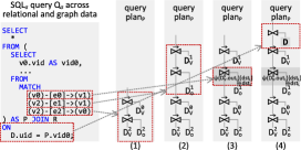
   Figure 12. A step-by-step demonstration of the parsing process from input ${\mathsf{SQL_{\delta}}}$ query to a logical query plan

   

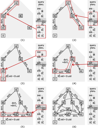
   Figure 13. A step-by-step demonstration of the query graph construction process from an input logical query plan

3. As both vertex $v0$ and $v1$ have already been considered in the query plan, the edge: $(v0)-[e0]\to(v1)$ will be parsed as an exploration condition: $\psi(D_{V}^{0}.out_{L})[dst_{L}]\ni dst_{L}$ and be incorporated into the operator: $R_{CSG_{C1}}{\vec{\bowtie}^{D_{V}^{2}.out_{L}}}_{\psi(D_{V}^{0}.out_{L})[dst_{L}]\ni dst_{L}}D_{o}^{1}$.

4. Parse the join on the relation $D$ as $R_{CSG_{C3}}\bowtie_{D_{V}^{0}.vid=uid}D$ on the top of the query plan generated so far, were $CSG_{C3}=\{D_{V}^{2},D_{o}^{2},D_{V}^{0},D_{o}^{1},D_{V}^{1}\}$.

C. Query Graph Construction

We provide a detailed, step-by-step demonstration in Figure 13 of the query graph construction process from $\text{Plan}_{\text{P}}$:

1. Each leaf node in the query plan will be constructed as a node in the query graph: $D$, $D_{V}^{1}$, $D_{o}^{1}$, $D_{V}^{0}$ $D_{o}^{2}$ and $D_{V}^{2}$.

2. An edge $(D_{V}^{2},out_{L},D_{o}^{2})$ will be constructed corresponding to the exploration operator: $D_{V}^{2}{\vec{\bowtie}^{out_{L}}}D_{o}^{2}$. Following that, an edge $(D_{o}^{2},dst_{L},D_{V}^{0})$ will be constructed corresponding to the exploration operator: $R_{CSG_{C0}}{\vec{\bowtie}^{D_{o}^{2}.dst_{L}}}D_{V}^{0}$.

3. An edge $(D_{V}^{2},out_{L},D_{o}^{1})$ will be constructed corresponding to the exploration operator: $R_{CSG_{C1}}{\vec{\bowtie}^{D_{V}^{2}.out_{L}}}D_{o}^{1}$. Following that, an edge $(D_{o}^{1},dst_{L},D_{V}^{1})$ will be constructed corresponding to the exploration operator: $R_{CSG_{C2}}{\vec{\bowtie}^{D_{o}^{1}.dst_{L}}}D_{V}^{1}$.

4. $D_{V}^{0}$ and $D$ will be connected with an edge that denotes the join: $D_{V}^{0}\bowtie_{vid=uid}D$.

5. Corresponding to the condition: $\psi(D_{V}^{0}.out_{L})[dst_{L}]\ni dst_{L}$, a node $D_{o}^{0}$ will be first inserted into the query graph and an edge $(D_{V}^{0},out_{L},D_{o}^{0})$ will be constructed. As $\mathcal{D}_{G}^{E}$ is in the regular form, it can be looked up that $D_{o}^{0}$ is an alias of $D_{o}$ as it is explored from the field $D_{V}^{0}[out_{L}]$. $D_{o}^{0}$ and $D_{o}^{1}$ will be further connected by an edge denoting the “same-pointer condition”: $D_{o}^{0}\bowtie_{dst_{L}=dst_{L}}D_{o}^{1}$.

6. According to the “same-pointer condition” $D_{o}^{0}\bowtie_{dst_{L}=dst_{L}}D_{o}^{1}$, we know that $D_{o}^{0}[dst_{L}]$ and $D_{o}^{1}[dst_{L}]$ point to the same tuple. Considering that there already exists an edge $(D_{o}^{1},dst_{L},D_{V}^{1})$, an edge $(D_{o}^{0},dst_{L},D_{V}^{1})$ will be constructed in the query graph.

7. All paths in the query graph that have the patterns:

   $$(D_{V})-[out_{L}]\to(D_{o})-[dst_{L}]\to(D_{V})$$

   $$(D_{V})-[in_{L}]\to(D_{i})-[src_{L}]\to(D_{V})$$

   will be recognized and duplicated oppositely. The rest “same pointer” conditions will then be completed, i.e., $D_{o}^{2}[dst_{L}]=D_{i}^{0}[src_{L}]$ and $D_{i}^{2}[src_{L}]=D_{i}^{1}[src_{L}]$.

D. Plan Enumeration

The “exploration” is represented as directed edge with an additional function $F$ in the extended query graph, for it to be still treated as an ordinary hyperedge in the plan enumeration process. Meanwhile, the “same pointer condition” will not be considered in the plan enumeration for exploring neighbouring nodes. That is, the edges with type “$\mathsf{duplicate}$” will be omitted when computing $N(v)$ and $N_{E}(v)$. They will only be used to resolve explorative condition.

However, as also mentioned in Section 5.3, there are several additional restrictions on the enumerated CSG-CMP pair for them to be resolves as exploration operator, like “duplicated nodes will not appear simultaneously”. In this case, the CSG-CMP pairs exported by previous plan enumeration methods we directly apply here can be illegal and break these restrictions. Here, we simply add a filter to verify the CSG-CMP pairs to get the legal ones without touching the details of the plan enumeration methods.

Input: Query graph $Q=(N,E,L,F)$, $CSG_{0},CSG_{1}\subseteq N$, and $D$.

Output: Boolean value $legal$.

// first check whether there are duplicated nodes

1for $n_{0}\in CSG_{0}$ do

      2 for $n_{1}\in CSG_{1}$ do

            3 if $\langle n_{0},n_{1}\rangle\in D$ or $\langle n_{1},n_{0}\rangle\in D$ then

                  4 return false

            

      

// then check whether these two CSGs are connected by exploration edge

5$e_{e}=null$ // to hold the exploration edge if it exists

6for $v\in CSG_{0}\cup CSG_{1}$ do

      7 for $e\in N_{E}(v)$ do

            

            8$\langle l,A\rangle=L(e)$ // to find exploration edge connects them

            9if $l\neq explore$ then

                  10 continue 

            

            11$\langle n_{s},n_{d}\rangle=F(e)$

            12if $n_{s}\in CSG_{0}$ and $n_{d}\notin CSG_{1}$ then

                  13 continue // inside $CSG_{0}$ or toward an outside vertex

            14if $n_{s}\in CSG_{1}$ and $n_{d}\notin CSG_{0}$ then

                  15 continue // inside $CSG_{1}$ or toward an outside vertex

            

            16if $e_{e}\neq null$ then

                  17 return false  // more than one exploration edge

            

            18$e_{e}=e$

      

19if $e_{e}=null$ then

       // the CSG-CMP pair is not connected by exploration edge

      20return true

21$\langle n_{s},n_{d}\rangle=F(e_{e})$

22if $n_{d}\in\{CSG_{0}\}$ and $|\{CSG_{0}\}|>1$ then

      23 return false  // toward the tuples in intermediate result

24if $n_{d}\in\{CSG_{1}\}$ and $|\{CSG_{1}\}|>1$ then

      25 return false  // toward the tuples in intermediate result

26return true

Algorithm 1 Legal CSG-CMP pair

Algorithm 1 shows such a filter. For an extended query graph $Q=(N,E,L,F)$, it accepts a CSG-CMP pair and a set denotes the duplicated nodes in $Q$: $D\subseteq N\times N$. As an example, for the query graph in Figure 6, $D=\bigcup_{k=0,1,2}\{\langle D_{o}^{k},D_{i}^{k}\rangle\}$. It can then return a boolean value to select all legal CSG-CMP pairs for operator resolution.

The example below shows that enumerating query plan in such an enlarged unified space allows the access on graph and relational data to be considered in any order.

Example 1.

We next provide a detailed step-by-step explanation to show how the query plans $\text{Plan}_{\text{RF}}$, $\text{Plan}_{\text{GF}}$ and $\text{Plan}_{\text{H}}$ in Figure 6 can be enumerated.

$\text{Plan}_{\text{RF}}$:

1. $CSG_{R0}\text{=}\{D_{V}^{0}\}\times CSG_{R1}\text{=}\{D\}$.

   Resolve to operator: $D_{V}^{0}\bowtie_{vid=uid}D$.

   As a plain value join operator.

2. $CSG_{R2}\text{=}CSG_{R0}\cup CSG_{R1}\text{=}\{D_{V}^{0},D\}\times CSG_{R3}\text{=}\{D_{o}^{0}\}$.

   Resolve to operator: $R_{CSG_{R2}}{\vec{\bowtie}^{D_{V}^{0}.out_{L}}}D_{o}^{0}$.

   As there is an edge: $(D_{V}^{0},out_{L},D_{o}^{0})$ from $CSG_{R2}$ toward $CSG_{R3}$.

3. $CSG_{R4}\text{=}CSG_{R2}\cup CSG_{R3}\text{=}\{D_{V}^{0},D,D_{o}^{0}\}\times CSG_{R5}\text{=}\{D_{V}^{1}\}$.

   Resolve to operator: $R_{CSG_{R4}}{\vec{\bowtie}^{D_{o}^{0}.dst_{L}}}D_{V}^{1}$.

   As there is an edge: $(D_{o}^{0},dst_{L},D_{V}^{1})$ from $CSG_{R4}$ toward $CSG_{R5}$.

4. $CSG_{R6}\text{=}CSG_{R4}\cup CSG_{R5}\text{=}\{D_{V}^{0},D,D_{o}^{0},D_{V}^{1}\}\times CSG_{R7}\text{=}\{D_{i}^{1}\}$.

   Resolve to operator: $R_{CSG_{R6}}{\vec{\bowtie}^{D_{V}^{1}.in_{L}}}_{\psi(D_{V}^{0}.in_{L})[src_{L}]\ni src_{L}}D_{i}^{1}$.

   As there is an edge: $(D_{V}^{1},in_{L},D_{i}^{1})$ from $CSG_{R6}$ toward $CSG_{R7}$, and a condition $D_{i}^{2}[src_{L}]\text{=}D_{i}^{1}[src_{L}]$ exists and an edge $(D_{V}^{0},in_{L},D_{i}^{2})$ explores from $CSG_{R6}$ to $D_{i}^{2}$, an explorative condition, $\psi(D_{V}^{0}.in_{L})[src_{L}]\ni src_{L}$, can then be incorporated into such an exploration.

5. $CSG_{R8}\text{=}CSG_{R6}\cup CSG_{R7}\text{=}\{D_{V}^{0},D,D_{o}^{0},D_{V}^{1},D_{i}^{1}\}\times CSG_{R9}\text{=}\{D_{V}^{2}\}$.

   Resolve to operator: $R_{CSG_{R8}}{\vec{\bowtie}^{D_{i}^{1}.src_{L}}}D_{V}^{2}$.

   As there is an outward edge: $(D_{i}^{1},src_{L},D_{V}^{2})$ from $CSG_{R8}$ toward $CSG_{R9}$.

$\text{Plan}_{\text{H}}$:

1. $CSG_{H0}\text{=}\{D_{V}^{0}\}\times CSG_{H1}\text{=}\{D_{o}^{0}\}$.

   Resolve to operator: $D_{V}^{0}{\vec{\bowtie}^{out_{L}}}D_{o}^{0}$.

   As there is an edge: $(D_{V}^{0},out_{L},D_{o}^{0})$ from $CSG_{H0}$ toward $CSG_{H1}$.

2. $CSG_{H2}\text{=}CSG_{H0}\cup CSG_{H1}\text{=}\{D_{V}^{0},D_{o}^{0}\}\times CSG_{H3}\text{=}\{D_{V}^{1}\}$.

   Resolve to operator: $R_{CSG_{H2}}{\vec{\bowtie}^{D_{o}^{0}.dst_{L}}}D_{V}^{1}$.

   As there is an edge: $(D_{o}^{0},dst_{L},D_{V}^{1})$ from $CSG_{H2}$ toward $CSG_{H3}$.

3. $CSG_{H4}\text{=}CSG_{H2}\cup CSG_{H3}\text{=}\{D_{V}^{0},D_{o}^{0},D_{V}^{1}\}\times CSG_{H5}\text{=}\{D\}$.

   Resolve to operator: $R_{CSG_{H4}}\bowtie_{D_{V}^{0}.vid=uid}D$.

   As a plain value join operator.

4. $CSG_{H6}\text{=}CSG_{H4}\cup CSG_{H5}\text{=}\{D_{V}^{0},D_{o}^{0},D_{V}^{1},D\}\times CSG_{H7}\text{=}\{D_{i}^{1}\}$.

   Resolve to operator: $R_{CSG_{H6}}{\vec{\bowtie}^{D_{V}^{1}.in_{L}}}_{\psi(D_{V}^{0}.in_{L})[src_{L}]\ni src_{L}}D_{i}^{1}$.

   As there is an edge: $(D_{V}^{1},in_{L},D_{i}^{1})$ from $CSG_{H6}$ toward $CSG_{H7}$, and a condition $D_{i}^{2}[src_{L}]\text{=}D_{i}^{1}[src_{L}]$ exists and an edge $(D_{V}^{0},in_{L},D_{i}^{2})$ explores from $CSG_{H6}$ to $D_{i}^{2}$, an explorative condition, $\psi(D_{V}^{0}.in_{L})[src_{L}]\ni src_{L}$, can then be incorporated into such an exploration.

5. $CSG_{H8}\text{=}CSG_{H6}\cup CSG_{H7}\text{=}\{D_{V}^{0},D_{o}^{0},D_{V}^{1},D,D_{i}^{1}\}\times CSG_{H9}\text{=}\{D_{V}^{2}\}$

   Resolve to operator: $R_{CSG_{H8}}{\vec{\bowtie}^{D_{i}^{1}.src_{L}}}D_{V}^{2}$.

   As there is an edge: $(D_{i}^{1},src_{L},D_{V}^{2})$ from $CSG_{H8}$ toward $CSG_{H9}$.

$\text{Plan}_{\text{GF}}$:

1. $CSG_{G0}\text{=}\{D_{V}^{2}\}\times CSG_{G1}\text{=}\{D_{o}^{1}\}$.

   Resolve to operator: $D_{V}^{2}{\vec{\bowtie}^{out_{L}}}D_{o}^{1}$.

   As there is an edge: $(D_{V}^{2},out_{L},D_{o}^{1})$ from $CSG_{G0}$ toward $CSG_{G1}$.

2. $CSG_{G2}\text{=}CSG_{G0}\cup CSG_{G1}\text{=}\{D_{V}^{2},D_{o}^{1}\}\times CSG_{G3}\text{=}\{D_{V}^{1}\}$.

   Resolve to operator: $R_{CSG_{G2}}{\vec{\bowtie}^{D_{o}^{1}.dst_{L}}}D_{V}^{1}$.

   As there is an edge: $(D_{o}^{1},dst_{L},D_{V}^{1})$ from $CSG_{G2}$ toward $CSG_{G3}$.

3. $CSG_{G4}\text{=}CSG_{G2}\cup CSG_{G3}\text{=}\{D_{V}^{2},D_{o}^{1},D_{V}^{1}\}\times CSG_{G5}\text{=}\{D_{o}^{2}\}$.

   Resolve to operator: $R_{CSG_{G4}}{\vec{\bowtie}^{D_{V}^{2}.out_{L}}}_{\psi(D_{V}^{1}.in_{L})[src_{L}]\ni dst_{L}}D_{o}^{2}$.

   As there is an edge: $(D_{V}^{2},out_{L},D_{o}^{2})$ from $CSG_{G4}$ toward $CSG_{G5}$, and a condition $D_{i}^{0}[src_{L}]\text{=}D_{o}^{2}[dst_{L}]$ exists and an edge $(D_{V}^{1},in_{L},D_{i}^{0})$ explores from $CSG_{G4}$ to $D_{i}^{0}$, an explorative condition, $\psi(D_{V}^{1}.in_{L})[src_{L}]\ni dst_{L}$, can then be incorporated into such an exploration.

4. $CSG_{G6}\text{=}CSG_{G4}\cup CSG_{G5}\text{=}\{D_{V}^{2},D_{o}^{1},D_{V}^{1},D_{o}^{2}\}\times CSG_{G7}\text{=}\{D_{V}^{0}\}$.

   Resolve to operator: $R_{CSG_{G6}}{\vec{\bowtie}^{D_{o}^{2}.dst_{L}}}D_{V}^{0}$.

   As there is an edge: $(D_{o}^{2},dst_{L},D_{V}^{0})$ from $CSG_{G6}$ toward $CSG_{G7}$.

5. $CSG_{G8}\text{=}CSG_{G6}\cup CSG_{G7}\text{=}\{D_{V}^{2},D_{o}^{1},D_{V}^{1},D_{o}^{2},D_{V}^{0}\}\times CSG_{G9}\text{=}\{D\}$.

   Resolve to operator: $R_{CSG_{G8}}\bowtie_{D_{V}^{0}.vid=uid}D$.

   As a plain value join operator.

This example is only to highlight the plan enumeration process, it will be shown below how the operators are resolved by accepting the corresponding CSG-CMP pair as input.

E. Cost Estimation

The example below provides an explanation of the cost estimation.

Example 2.

For the query plan $\text{Plan}_{\text{RF}}$, $\text{Plan}_{\text{GF}}$ and $\text{Plan}_{\text{H}}$ in Figure 6, we then provide a step-by-step explanation of how their cost can be estimated with the cost model $C_{emm}$ in Section 5.3.

$\text{Plan}_{\text{RF}}$:

$$C_{emm}(CSG_{R2})= \tau|D_{V}^{0}|+\tau|D|+|R_{CSG_{R2}}|$$

$$C_{emm}(CSG_{R4})= C_{emm}(CSG_{R2})+\tau|R_{CSG_{R2}}[D_{V}^{0}.out_{L}]|$$

$$C_{emm}(CSG_{R6})= C_{emm}(CSG_{R4})+\tau|R_{CSG_{R4}}[D_{o}^{0}.dst_{L}]|$$

$$= C_{emm}(CSG_{R4})+\tau|R_{CSG_{R4}}|$$

$$C_{emm}(CSG_{R8})= C_{emm}(CSG_{R6})+\tau|R_{CSG_{R6}}[D_{V}^{1}.in_{L}]|$$

$$+\tau{|\Pi_{D_{V}^{0}.in_{L}}R_{CSG_{R6}}[D_{V}^{0}.in_{L}]|}+|R_{CSG_{R8}}|$$

$$C_{emm}(\text{Plan}_{\text{RF}})= C_{emm}(CSG_{R8})+\tau|R_{CSG_{R8}}[D_{i}^{1}.src_{L}]|$$

$$= C_{emm}(CSG_{R8})+\tau|R_{CSG_{R8}}|$$

$$= (1+\tau)|R_{CSG_{R8}}|+\tau|R_{CSG_{R6}}[D_{V}^{1}.in_{L}]|$$

$$+\tau{|\Pi_{D_{V}^{0}.in_{L}}R_{CSG_{R6}}[D_{V}^{0}.in_{L}]|}+\tau|R_{CSG_{R4}}|$$

$$+\tau|R_{CSG_{R2}}[D_{V}^{0}.out_{L}]|+|R_{CSG_{R2}}|+\tau|D_{V}^{0}|+\tau|D|$$

$\text{Plan}_{\text{H}}$:

$$C_{emm}(CSG_{H2})= \tau|D_{V}^{0}|+\tau|D_{V}^{0}[out_{L}]|$$

$$C_{emm}(CSG_{H4})= C_{emm}(CSG_{H2})+\tau|R_{CSG_{H2}}[D_{o}^{0}.dst_{L}]|$$

$$= C_{emm}(CSG_{H2})+\tau|R_{CSG_{H2}}|$$

$$C_{emm}(CSG_{H6})= C_{emm}(CSG_{H4})+\tau|D|+|R_{CSG_{H6}}|$$

$$C_{emm}(CSG_{H8})= C_{emm}(CSG_{H6})+\tau|R_{CSG_{H6}}[D_{V}^{1}.in_{L}]|$$

$$+\tau{|\Pi_{D_{V}^{0}.in_{L}}R_{CSG_{H6}}[D_{V}^{0}.in_{L}]|}+|R_{CSG_{H8}}|$$

$$C_{emm}(\text{Plan}_{\text{H}})= C_{emm}(CSG_{H8})+\tau|R_{CSG_{H8}}[D_{i}^{1}.src_{L}]|$$

$$= C_{emm}(CSG_{H8})+\tau|R_{CSG_{H8}}|$$

$$= (1+\tau)|R_{CSG_{H8}}|+\tau|R_{CSG_{H6}}[D_{V}^{1}.in_{L}]|$$

$$+\tau{|\Pi_{D_{V}^{0}.in_{L}}R_{CSG_{H6}}[D_{V}^{0}.in_{L}]|}+|R_{CSG_{H6}}|$$

$$+\tau|R_{CSG_{H2}}|+\tau|D_{V}^{0}[out_{L}]|+\tau|D_{V}^{0}|+\tau|D|$$

$\text{Plan}_{\text{GF}}$:

$$C_{emm}(CSG_{G2})= \tau|D_{V}^{2}|+\tau|D_{V}^{2}[out_{L}]|$$

$$C_{emm}(CSG_{G4})= C_{emm}(CSG_{G2})+\tau|R_{CSG_{G2}}[D_{o}^{1}.dst_{L}]|$$

$$= C_{emm}(CSG_{G2})+\tau|R_{CSG_{G2}}|$$

$$C_{emm}(CSG_{G6})= C_{emm}(CSG_{G4})+\tau|R_{CSG_{G4}}[D_{V}^{2}.out_{L}]|$$

$$+\tau{|\Pi_{D_{V}^{1}.in_{L}}R_{CSG_{G4}}[D_{V}^{1}.in_{L}]|}+|R_{CSG_{G6}}|$$

$$C_{emm}(CSG_{G8})= C_{emm}(CSG_{G6})+\tau|R_{CSG_{G6}}[D_{o}^{2}.dst_{L}]|$$

$$= C_{emm}(CSG_{G6})+\tau|R_{CSG_{G6}}|$$

$$C_{emm}(\text{Plan}_{\text{GF}})= C_{emm}(CSG_{G8})+\tau|D|+|R_{CSG_{G8}}|$$

$$= |R_{CSG_{G8}}|+(1+\tau)|R_{CSG_{G6}}|+\tau|R_{CSG_{G4}}[D_{V}^{2}.out_{L}]|$$

$$+\tau{|\Pi_{D_{V}^{1}.in_{L}}R_{CSG_{G4}}[D_{V}^{1}.in_{L}]|}$$

$$+\tau|R_{CSG_{G2}}|+\tau|D|+\tau|D_{V}^{2}|+\tau|D_{V}^{2}[out_{L}]|$$

As a simplification, for all relation $T$ and their field $A$, we assume $|\Pi_{A}(T)|\approx|T|$. Meanwhile, for arbitrary relations $T$ and $T^{\prime}$, and pointer field $p$ in $T^{\prime}$, we assume $|T[T^{\prime}.p]|\approx|T|\frac{|T^{\prime}[p]|}{|T^{\prime}|}$, which also implies the simple histogram method we utilized to estimate the “selectivity” of exploration.

We then have:

$$C_{emm}(\text{Plan}_{\text{RF}})\approx (1+\tau)|R_{CSG_{R8}}|$$

$$+\tau|R_{CSG_{R6}}|(\frac{|D_{V}^{1}[in_{L}]|}{|D_{V}^{1}|}+\frac{|D_{V}^{0}[in_{L}]|}{|D_{V}^{0}|})+\tau|R_{CSG_{R4}}|$$

$$+|R_{CSG_{R2}}|(1+\tau\frac{|D_{V}^{0}[out_{L}]|}{|D_{V}^{0}|})+\tau|D_{V}^{0}|+\tau|D|$$

$$C_{emm}(\text{Plan}_{\text{H}})\approx (1+\tau)|R_{CSG_{H8}}|$$

$$+|R_{CSG_{H6}}|(\tau\frac{|D_{V}^{1}[in_{L}]|}{|D_{V}^{1}|}+\tau\frac{|D_{V}^{0}[in_{L}]|}{|D_{V}^{0}|}+1)$$

$$+\tau|R_{CSG_{H2}}|+\tau|D_{V}^{0}|(1+\frac{|D_{V}^{0}[out_{L}]|}{|D_{V}^{0}|})+\tau|D|$$

$$C_{emm}(\text{Plan}_{\text{GF}})\approx |R_{CSG_{G8}}|+(1+\tau)|R_{CSG_{G6}}|$$

$$+\tau|R_{CSG_{G4}}|(\frac{|D_{V}^{1}[in_{L}]|}{|D_{V}^{1}|}+\frac{|D_{V}^{2}[out_{L}]|}{|D_{V}^{2}|})$$

$$+\tau|R_{CSG_{G2}}|+\tau|D_{V}^{2}|(1+\frac{|D_{V}^{2}[out_{L}]|}{|D_{V}^{2}|})+\tau|D|$$

To actually compute such a cost, we then specify a set of statistics, one can verify that there exists a data set that satisfies them especially when there are pulled down filter conditions for label checking contained in these nodes in the query graph:

$$|R_{CSG_{R8}}|=|R_{CSG_{H8}}|=|R_{CSG_{G8}}|=10^{4}$$

$$|R_{CSG_{R6}}|=|R_{CSG_{H6}}|=|R_{CSG_{G6}}|=2\times 10^{3}$$

$$|R_{CSG_{R4}}|=2\times 10^{5},\;|R_{CSG_{G4}}|=10^{4}$$

$$|R_{CSG_{R2}}|=|R_{CSG_{H2}}|=10^{4},\;|R_{CSG_{G2}}|=10^{3}$$

$$\frac{|D_{V}^{0}[in_{L}]|}{|D_{V}^{0}|}=\frac{|D_{V}^{0}[out_{L}]|}{|D_{V}^{0}|}=\frac{|D_{V}^{1}[in_{L}]|}{|D_{V}^{1}|}=\frac{|D_{V}^{2}[out_{L}]|}{|D_{V}^{2}|}=100$$

$$|D_{V}^{0}|=|D_{V}^{2}|=|D|=10^{3}$$

Then, there are:

$C_{emm}(\text{Plan}_{\text{H}})\approx 0.34\;C_{emm}(\text{Plan}_{\text{RF}})\approx 0.27\;C_{emm}(\text{Plan}_{\text{GF}})$

That is, on this set of data with this designated query, the plan $\text{Plan}_{\text{H}}$ has the lowest cost as it pulls the join on relation down to the pattern matching process.

F. Operator Resolution

The above discussions are all about CSG and will generate a tree of them that representing the optimized join order. According to the query optimization workflow, a query plan will then be resolved corresponding to it. The crucial points for the operator resolution process here to departure from its counterpart for conventional relational operator are highlighted in Section 5.3. Below is an overall description of the entire resolution process.

Input: Query graph $Q=(N,E,L,F)$, $CSG_{0},CSG_{1}\subseteq N$.

Output: Operator $op$.

// resolve explorative join condition, as $\mathsf{ResolveExp}$ can only consider exploration condition in only direction

1$\theta=\text{{$\mathsf{ResolveExp}$}}(CSG_{0},CSG_{1})\cup\text{{$\mathsf{ResolveExp}$}}(CSG_{1},CSG_{0})$

// resolve plain value join condition, $\mathsf{ResolveCond}$ can consider the condition from two directions

// will not consider the edges with type $\mathsf{duplicate}$

2$\theta=\theta\cup\text{{$\mathsf{ResolveCond}$}}(CSG_{0},CSG_{1})$

// resolve operator, find whether these two CSGs are connected by an exploration edge

3$e_{e}=null$ // to hold the exploration edge if it exists

4for $v\in CSG_{0}\cup CSG_{1}$ do

      5 for $e\in N_{E}(v)$ do

            

            6$\langle l,A\rangle=L(e)$

            7if $l\neq explore$ then

                  8 continue 

            

            9$\langle n_{s},n_{d}\rangle=F(e)$

            10if $n_{s}\in CSG_{0}$ and $n_{d}\notin CSG_{1}$ then

                  11 continue // inside $CSG_{0}$ or toward an outside vertex

            12if $n_{s}\in CSG_{1}$ and $n_{d}\notin CSG_{0}$ then

                  13 continue // inside $CSG_{1}$ or toward an outside vertex

            

            14$e_{e}=e$

      

15if $e_{e}=null$ then

      

      16return $R_{CSG_{0}}\bowtie_{\theta}R_{CSG_{1}}$ // is a plain value join

17$\langle l,A\rangle=L(e_{e})$, $\langle n_{s},n_{d}\rangle=F(e_{e})$ // is an exploration

18if $n_{s}\in CSG_{0}$ then

      19 return $R_{CSG_{0}}{\vec{\bowtie}^{A}}_{\theta}R_{CSG_{1}}$

20return $R_{CSG_{1}}{\vec{\bowtie}^{A}}_{\theta}R_{CSG_{0}}$

Algorithm 2 $\mathsf{ResolveOp}$

$\mathsf{ResolveOp}$ in Algorithm 2 describes the overall operator resolution process, where the aggression is omitted. By accepting a CSG-CMP pair as input, explorative conditions and plain value join conditions will be first resolved, by calling $\mathsf{ResolveExp}$ and $\mathsf{ResolveCond}$ respectively. After that, an operator will be generated according to the edges connect the two CSGs and be integrated with the resolved conditions. That is, if the two input CSGs are connected by an exploration edge, an exploration operator will then be resolved. Otherwise, a plain-value join operator will be resolved. Meanwhile, it should be noticed that according to the query graph construction process and the CSG-CMP pairs filter atop of the plan enumeration method, any two CSGs that are considered for operator resolution here can only be connected by a single exploration edge or several edges for plain join conditions.

We then show how the explorative conditions can be resolved according to the input CSG-CMP pair through $\mathsf{ResolveExp}$ in Algorithm 3. Corresponding to the description in Section 5.3, outward edges from one CSG will be first explored to find the nodes not contained in both CSGs. For these explored nodes, it will be checked whether there are edges connecting them to the other CSG. If so, those edges will be considered as explorative join conditions. The $\mathsf{ResolveCond}$ resolves plain join conditions along the same line as its relational counterpart and will not be further explained here.

With the above operator resolution process, a logical query plan can then be rewritten from the optimized CSG tree accordingly.

Input: Query graph $Q=(N,E,L,F)$, $CSG_{0},CSG_{1}\subseteq N$.

Output: Explorative condition set $\theta^{I}$.

1$\theta^{I}=\{\}$

2for $n_{0}\in CSG_{0}$ do

      3 for $e\in N_{E}(n_{0})$ do

            

            4$\langle l,A\rangle=L(e)$

            5if $l\neq{\mathsf{explore}}$ then

                  6 continue // is not an exploration edge

            

            7$\langle n_{s},n_{d}\rangle=F(e)$

            8if  $n_{d}\in CSG_{0}\cup CSG_{1}$ then

                  9 continue // has already been considered

            // to find the edges connect $n_{d}$ and nodes in $CSG_{1}$

            10for $e_{c}\in N_{E}(n_{d})$ do

                  

                  11$\langle l_{c},A_{c}\rangle=L(e_{c})$

                  12if $l_{c}={\mathsf{explore}}$ then

                        13 continue 

                  

                  14if $N(e_{c})\subseteq CSG_{1}\cup\{n_{d}\}$ then

                         // $e_{c}$ can be resolved as explorative join condition

                        15$\theta^{I}=\theta^{I}\cup\{\psi(A)[A_{c}]\ni A_{c}\}$

                  

            

      

16return $\theta^{I}$

Algorithm 3 $\mathsf{ResolveExp}$

G. Query Execution

Introducing the exploration operator into the query plan allows the access on graph and relational data to be executed seamlessly without switching to another execution engine to avoid performance degradation, instead of merely satisfying a taste of elegance.

A typical example is demonstrated in Figure 6 but was not clearly explained in Section 5.3 due to the limitation of space, which will be explained with a step-by-step example here in detail.

Example 3.

Considering the three stages of the pipelined execution for $\text{Plan}_{\text{H}}$ in Figure 6, that access across the relational and graph data without breaking the pipelined execution process.

1. In $\text{stage}_{\text{1}}$, an exploration operator $R_{CSG_{H2}}{\vec{\bowtie}^{D_{o}^{0}.dst_{L}}}D_{V}^{1}$ is executed. Field $D_{o}^{0}.dst_{L}$ is held in the pipeline intermediate result $R_{CSG_{H2}}$ which points to relation $D_{V}^{1}$. During the exploration process, all tuples $t_{H2}\in R_{CSG_{H2}}$ will be explored to iterate over all tuples $t_{V}^{1}\in\psi(t_{H2}[D_{o}^{0}.dst_{L}])\subseteq D_{V}^{1}$ to grab field $t_{V}^{1}[in_{L}]$ into the next stage of the pipelined intermediate result till it is filled.

2. In $\text{stage}_{\text{2}}$, an ordinary join operator $R_{CSG_{H4}}\bowtie_{D_{V}^{0}.vid=D.uid}D$ is executed. Field $D_{V}^{0}.vid$ is held in the pipeline intermediate result $R_{CSG_{H4}}$. All tuples $t_{H4}\in R_{CSG_{H4}}$ will then be iterated, to join on all tuples $t_{R}\in D$ s.t. $t_{H4}[D_{V}^{0}.vid]=t_{R}[uid]$.

3. In $\text{stage}_{\text{3}}$, an intersective exploration operator is executed, $R_{CSG_{H6}}{\vec{\bowtie}^{D_{V}^{1}.in_{L}}}_{\psi(D_{V}^{0}.in_{L})[src_{L}]\ni src_{L}}D_{i}^{1}$, to continue the pattern matching process. Field $D_{V}^{0}.in_{L}$ and $D_{V}^{1}.in_{L}$ are held in the pipeline intermediate result $R_{CSG_{H6}}$. All tuples $t_{H6}\in R_{CSG_{H6}}$ will be iterated, to intersect all tuples $t_{i}^{2}\in\psi(t_{H6}[D_{V}^{0}.in_{L}])\subseteq D_{i}^{2}$ and $t_{i}^{1}\in\psi(t_{H6}[D_{V}^{1}.in_{L}])\subseteq D_{i}^{1}$, s.t. $t_{i}^{1}[src_{L}]=t_{i}^{2}[src_{L}]$.

In the external level, it can be seen that $\text{stage}_{\text{1}}$ to $\text{stage}_{\text{3}}$ explore the graph data, relational data and back to the graph data subsequently without breaking the pipelined execution.

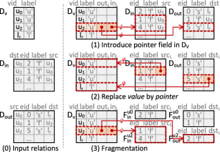
Figure 14. A step-by-step demonstration of the conversion process from relations to $\mathsf{RG}$ model

H. Graph Representation in RG Model

The example below provides a detailed explanation to illustrate how graph-structured data can be represented in the $\mathsf{RG}$ model. Different from the description in Section 4.1 for encoding graph-structured data, the example here offers a (conceptional) conversion process from a relational representation of the graph data, to emphasize the extensions that the $\mathsf{RG}$ model introduces into the relational model.

Example 4.

Taking $G$ in Figure 1 as an example, Figure 14 provides a step-by-step explanation to store the graph $G$ in the $\mathsf{RG}$ model from a relational representation of it. As a simplification, we do not consider the property on both vertices and edges here.

1. The relational representation of $G$ consists of three relations: $\mathsf{D_{V}(vid,label)}$ to hold all vertices in $G$; $\mathsf{D_{in}(dst,eid,label,src)}$ to hold all edges in $G$; $\mathsf{D_{out}(src,eid,label,dst)}$, as a duplication of $\mathsf{D_{in}}$, or a virtual view of it.

2. Add pointer field $out_{L}$ (resp. $in_{L}$) into $D_{V}$ to connect to all outward (resp. input) edges for each vertex in it, which makes it become $\mathsf{D_{V}(vid,label,out_{L},in_{L})}$. Field $src$ in $D_{in}$ and $dst$ in $D_{out}$ can then be removed, for them to become $\mathsf{D_{in}(eid,label,dst)}$ and $\mathsf{D_{out}(src,eid,label)}$ respectively. It thence reduces the duplication between $D_{in}$ and $D_{out}$.

3. Replace the field $src$ in $D_{in}$ (resp. $dst$ in $D_{out}$) as $src_{L}$ (resp. $dst_{L}$), that is, for each tuple $t\in D_{in}$ (resp. $t\in D_{out}$), replace the value of its field $t[src]\in\mathbb{V}$ (resp. $t[dst]\in\mathbb{V}$) with pointer $t[src_{L}]\in\mathbb{P}$ (resp. $t[dst_{L}]\in\mathbb{P}$) towards the same vertex tuple. We can then get $\mathsf{D_{in}(eid,label,dst_{L})}$ and $\mathsf{D_{out}(src_{L},eid,label)}$.

4. Fragment the extended relation $D_{in}$ and $D_{out}$ according to the pointers in $out_{L}$ and $in_{L}$ in $D_{V}$, as mentioned in Section 4.1.

One can verify that the $\mathsf{RG}$ representation obtained in the above process is equivalent to the one resulted in Example 2.

It should be noticed that the extended relations $D_{\mathsf{V}}$, $D_{\mathsf{out}}$, $D_{\mathsf{in}}$ and the dereference function $\psi$ in $\mathcal{D}_{G}^{E}$ have actually already been obtained at $\text{stage}_{\text{2}}$. The following $\text{stage}_{\text{3}}$ is only to complete the fragmentation to support an efficient exploration through the pointer. It is also noteworthy that the fragmentation performed in $\text{stage}_{\text{3}}$ is actually at the logical level, without specifying the memory layout or the physical designs.

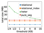
(a) $\mathsf{DBLP}$

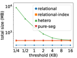
(b) $\mathsf{IMDB}$

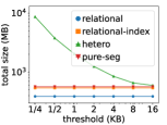
(c) $\mathsf{YAGO}$

Figure 15. Heterogeneous fragment storage estimation

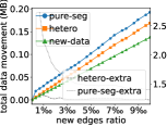
(a) $\mathsf{DBLP}$

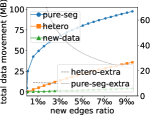
(b) $\mathsf{IMDB}$

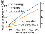
(c) $\mathsf{YAGO}$

Figure 16. Incremental data movement estimation

Meanwhile, it can also be clearly verified here that the $\mathcal{D}_{G}^{E}$ is in the regular form. That is, all pointers in field $out_{L}$ (resp. $in_{L}$) of $D_{V}$ reference to the tuples in $D_{out}$ (resp. $D_{in}$); the pointers in both fields $src_{L}$ (resp. $dst_{L}$) of $D_{in}$ (resp. $D_{out}$) all point to tuple in $D_{V}$. Therefore, given a pointer $p\in\mathbb{P}$, the relation that holds $\psi(p)$ can be looked-up according to the underlying field of $p$. A node can then be introduced into the query graph as an alias of that relation to correspond to the explorative condition as in Appendix C.

I. Evaluation on Memory Management

We evaluated the proposed heterogeneous fragment management strategy, on its storage cost and maintenance cost.

Exp-6: Storage cost. As described in Section 4, the extended relations need to be fragmented to efficiently support the exploration of a set of tuples. However, such a process will inevitably introduce additional costs, including the storage for the additional pointer fields and the internal fragmentation inside a block. We evaluated the cost introduced by the heterogeneous fragment management strategy, denoted as $\mathsf{hetero}$, with the following four kinds of baseline: (1) $\mathsf{relational}$, stores graph data in vertex relation $D_{V}(vid,label)$ and edge relation $D_{E}(eid,src,label,dst)$; (2) $\mathsf{relational\text{-}index}$, further considers two indexes on $src$ and $dst$ field on the edge relation $D_{E}$ respectively; (3) $\mathsf{pure\text{-}seg}$, stores graph data in the $\mathsf{RG}$ model and treats all fragments as segments, even the very large ones, and will not divide them into blocks; (4) $\mathsf{pure\text{-}block}$, stores graph data in the $\mathsf{RG}$ model and allocates at least one block for each fragment. We set the block size as $\mathsf{64KB}$ and varied the predefined block-segment threshold for heterogeneous fragment management mentioned in Section 4.2, to evaluate the cost introduced in such a process.

Evaluated with real-life data, we demonstrated in Figure 15 that storing graph data in the $\mathsf{RG}$ model with the $\mathsf{pure\text{-}seg}$ setting took 51.5%, 49.9% and 46.1% additional space on $\mathsf{DBLP}$, $\mathsf{IMDB}$ and $\mathsf{YAGO}$ respectively compared to the $\mathsf{relational}$ baseline. However, when taking the storage for the indexes data into account, i.e., comparing $\mathsf{pure\text{-}seg}$ to $\mathsf{relational\text{-}index}$, the additional space required on them would be reduced to 9.08%, 5.01% and 6.52% respectively. It should be noticed that the indexes on edge relation took a large portion of the storage since we did not considered heavy property on both vertex and edge in the graph data. Considering the two additional indexes is equivalent to consider the columns $src$ and $dst$ in the edge relation twice which can largely increase the required space. Therefore, it can be seen that the space utilized for storing graph data in the $\mathsf{RG}$ model is basically equivalent to storing the same set of data in relations and then add indexes on them.

We then vary the predefined block-segment threshold to evaluate the extra storage cost that the internal fragmentation in the heterogeneous memory management strategy can bring. As shown in Figures 15(a) to 15(c) , when the threshold is set to $\mathsf{8}$ KB, i.e., the fragments smaller than $\mathsf{8}$ KB will all be managed as segments, $\mathsf{hetero}$ took 24.5%, 11.5% and 21.7% additional space compared to $\mathsf{pure\text{-}seg}$ on these three data graphs respectively. Meanwhile, the heterogeneous management also significantly reduced (¡ 1/100) the space required for the $\mathsf{pure\text{-}block}$ strategy (not drawn).

Exp-7: Maintenance cost. We then evaluated the maintenance cost and the reduction of data movement amount achieved by the heterogeneous fragment management strategy. For each data graph $G$, we generated a $\Delta G$ on it and compared the data movement amount required to accept such an update by the heterogeneous fragment management strategy, denoted as $\mathsf{hetero}$, with two kinds of baselines: (1) in $\mathsf{new\text{-}data}$, we simply calculated the size of new inserted edges; (2) in $\mathsf{pure\text{-}seg}$, we calculated the data movement amount required when all fragments are managed as segments, where all introduced edges would uniformly require their underlying segments to be reallocated. We also estimated the ratio of extra data movement required by these two strategies, i.e., compared $\mathsf{hetero}$ and $\mathsf{pure\text{-}seg}$ to $\mathsf{new\text{-}data}$, denoted as $\mathsf{hetero\text{-}extra}$ and $\mathsf{pure\text{-}seg\text{-}extra}$ respectively.

Figure 16 shows the data movement amount required for segment reallocation when different amounts of new edges were inserted into the data graph that had been stored in the $\mathsf{RG}$ model. Owing to their topological characteristics, it can be seen that the data movement amount in $\mathsf{pure\text{-}seg}$ baseline were not extraordinarily larger than the $\mathsf{new\text{-}data}$ on both $\mathsf{DBLP}$ and $\mathsf{YAGO}$. That is, on these two data graphs, the introduced edges were all added into the relatively small fragments and thus does not introduce much extra data movement. However, the situation is completely different on $\mathsf{IMDB}$, as the introduced edges can easily connect to vertices with a large degree, the required data movement to reallocate the underlying segment thence becomes unacceptable even with only a very few edges inserted. Meanwhile, on all data graphs, the ratio of extra data movement required in both fragment management strategises were reduced as the number of inserted edges increases. This is due to the size of the tuples inserted into the segments is becoming comparable to the data that these segments originally held.

The experimental result shows that the heterogeneous memory management strategy can significantly reduce the extra data movement enforced by introducing a small amount of edges. With the block size set to $\mathsf{64KB}$ and the predefined block-segment threshold set to $\mathsf{8KB}$, such a strategy can reduce the extra data movement in $\mathsf{pure\text{-}seg\text{-}extra}$ by 1.71x, 9.49x and 1.54x on these three data graphs respectively when 1‰ new edges are inserted into them. Combining with the storage cost estimated in Exp-6, it can be seen that such a heterogeneous strategy fairly achieved a trade-off between these two strategies. We defer an in-depth study to apply more advanced dynamic memory management strategies (Wilson et al., 1995) to future work to further reduce the extra data movement here.

J. Notation Collection

We collect the frequent used notations in Table 2, ordered by the location of their first appearance.

	Notation	Conception
Section 2	$\mathbb{V}$	domain of plain values
	$P[\bar{A}](G)$	graph pattern query
	$\bowtie_{\delta}$	join on semantic connection
	${\mathsf{RA_{\delta}}}$	proposed relational algebra dialect
	${\mathsf{SQL_{\delta}}}$	proposed $\mathsf{SQL}$ dialect
Section 4.1	$\mathbb{P}$	domain of pointers
	${\mathcal{R}}^{E}$	$\mathsf{RG}$ schema
	$\mathcal{D}^{E}$	extended database
	$\phi$	injective partial reference function
	$\psi$	dereference function
	${\mathcal{R}}^{E}_{G}$	$\mathsf{RG}$ schema of graph $G$
	$\mathcal{D}_{G}^{E}$	extended relation of graph $G$
	$D_{\mathsf{V}}$	extended relation of vertices
	$D_{\mathsf{out}}$	extended relation of outgoing edges
	$D_{\mathsf{in}}$	extended relation of incoming edges
	$F^{v}_{\mathsf{out}}$	fragment of $D_{\mathsf{out}}$ of all outgoing edges from $v$
	$F^{v}_{\mathsf{in}}$	fragment of $D_{\mathsf{in}}$ of all incoming edges toward $v$
Section 5.1	$\theta^{I}$	notation of explorative condition
	$\psi(A)[B]\ni C$	form of an explorative condition
	$S_{1}\vec{\bowtie}^{A}_{\theta}S_{2}$	the (logical) exploration operator
	$S_{1}\>{\bowtie}_{\theta^{I}}S_{2}$	the (logical) join with explorative condition
	$S_{1}\>\vec{\bowtie}^{A}_{\theta^{I}}S_{2}$	the (logical) intersective exploration
Section 5.3	$(S_{1},A,S_{2})$	form of an exploration edge
	$|S|$	cardinality estimated for relation $S$
	$|S[A]|$	cardinality estimated for data linked by field $A$ in $S$
	$C(v_{i})$	candidate set generated for pattern vertex $v_{i}$
	$D^{C}_{v_{i}}$	separated relation to store $C(v_{i})$

Table 2. Summary of notations

Level	Relational Model		Relational Genetic Model		Graph Model
	structural	operational	structural	operational	structural	operational
External	relational views	$\mathsf{SQL}$ etc.	relational views + graph views	${\mathsf{SQL_{\delta}}}$	graph views	graph query languages
Logical	base relations	logical operators	extended relations	logical operators + exploration	base graphs	logical graph operators
Physical	physical designs	physical operators	physical designs + pointers	physical operators + exploration	physical designs for graph	physical graph operators

Table 3. A comparison of different data models under the perspective of the three level architecture

K. Query Language Comparison

Again, instead of providing a fully-featured and well-standardised query language for the community to follow, ${\mathsf{SQL_{\delta}}}$ is proposed here mainly as a demo language to verify the concept of hybrid queries across graph and relational data, and also to make our discussions on query evaluation more concentrated. It should also be noted again that such a language is defined on the external-level of the $\mathsf{RG}$ model as shown in Figure 2 and Table 3, where the introduced logical-level pointers are hidden to avoid introducing unacceptable complexity.

However, by saying that ${\mathsf{SQL_{\delta}}}$ is a demo language, we do not mean that it is overly simplified and overlooks the key features of various graph query languages, or is in an unusable shape. In fact, a large portion of those features provided by various graph query languages are equivalently achieved in ${\mathsf{SQL_{\delta}}}$ by combing few key features from both the graph-side and relational-side query languages. The most significant limitation on the expressiveness of ${\mathsf{SQL_{\delta}}}$ appears in the lack of support for the recursive feature, which is far beyond the scope that can be discussed here but can have some alternative temporary solution and will be systemically studied in future work.

Below, we compare the expressiveness and the usability of ${\mathsf{SQL_{\delta}}}$ with some graph query languages:

Expressiveness. Following the same categorisation of query features and semantics in (Angles et al., 2017), we first compare the expressiveness of ${\mathsf{SQL_{\delta}}}$ with other graph query languages. We listed the comparison on pattern matching queries and navigational queries in Table 4 and Table 5 respectively. Meanwhile, although they are not collected in the same table, considering the connection between the RDF model and the relational model, it can be seen that the other graph algebras built atop of the relational model (Zhao and Yu, 2017) can, at most, achieve an equivalent expressiveness as SPARQL.

Comparing to the various graph query languages, the most significant limitations of ${\mathsf{SQL_{\delta}}}$ appear on the navigational queries, since it can only describe the path with fixed-length patterns which might even hard to be called a real “navigational” query. The navigational queries in those graph query languages are mainly described by path with different kinds of regular expressions, which can be, and can only be, equivalently achieved in $\mathsf{SQL}$ with a recursive extension (Sakr et al., 2021). Although a consideration of the recursive features is far beyond the scope that can be discussed here, previous works (Jindal et al., 2015) also provide an alternative way to support recursive exploration, i.e., repeatedly running a script until it reaches a fixed point. However, such an approach is only a temporary solution and is far from considering all the optimization methods available for recursive relational queries (Bancilhon et al., 1985), we thus defer a systemic study on this to further work.

In conclusion, as a demo language to prove the concept of hybrid query across graph and relational data, ${\mathsf{SQL_{\delta}}}$ can fairly express the core concepts of the graph query languages especially on pattern queries. Meanwhile, the limitations on navigational queries in ${\mathsf{SQL_{\delta}}}$ can have some temporary solutions as in (Jindal et al., 2015), and a systematic study on this can be achieved by incorporating more classical works on recursive relational queries (Bancilhon et al., 1985), which is deferred to future work.

Usability. We further analysis the usability of such a demo language, more specifically, on its composability, ease of pattern specification, and simplicity of its query interface.

Composability. The composability is to say that the output of a query can be used as the input of another query, which is overlooked by the graph query languages in the early stage (W3C Recommendation, 2008; van Rest et al., 2016). The recent query languages (Angles et al., 2018), and recent versions of some evolving query languages (Francis et al., 2018), achieve such a property in different ways by exporting the result of a query as a graph (Angles et al., 2018) or passing “table-graphs” (Francis et al., 2018). As a dialect of $\mathsf{SQL}$, ${\mathsf{SQL_{\delta}}}$ then naturally retains its capability of query composition, that is, it can naturally export the result of the query on the graph-side data as relations for it to be regarded as the input of another query.

Pattern specification. There are majorly three styles to specify the pattern to be matched on data graph in previous graph query languages, namely, the “SQL-like” style (W3C Recommendation, 2008); the “functional” style (Tin, 2017); and the “ASCII-art” style (39075, 2023; 9075-16, 2022; Angles et al., 2018; Deutsch et al., 2022; Francis et al., 2023, 2018; van Rest et al., 2016). Among them, the “ASCII-art” style is undoubtedly the easiest-to-use and the most widely-recognized one in the community of graph query language, as it is utilized in a major portion of the query languages from both academia and industry, which is thus followed in ${\mathsf{SQL_{\delta}}}$.

Query interface. An important lesson learnt from the “great battle” between the relational and the CODASYL model (Bachman et al., 1969) is that the complicated structures is almost impossible for the practitioners to understand (Stonebraker and Hellerstein, 2005). Therefore, in $\mathsf{RG}$ model, as shown in Figure 2, the similar pointer structures are introduced, but they only appear on the logical level and are hidden from the external view. That is, for the practitioners who are trying to query on the data by writing declarative queries, they can only view on the certain relations and certain graphs, without seeing the extended relations with complicated pointer structures behind them on logical level.

Language	Supported patterns	Semantics
SPARQL (W3C Recommendation, 2008)	all complex graph patterns	homomorphism-based, bags
Cypher (Francis et al., 2018)	all complex graph patterns	no-repeated-edges, bags
Gremlin (Tin, 2017)	all complex graph patterns without explicit optional	homomorphism-based, bags
${\mathsf{SQL_{\delta}}}$	all complex graph patterns	homomorphism-based, bags

Table 4. A comparison of semantics for pattern matching

Language	Path expressions	Semantics	Choice of output
SPARQL	more than RPQs	arbitrary paths, sets	boolean / nodes
Cypher	fragment of RPQs	no repeated edges, bags	boolean / nodes / paths / graphs
Gremlin	more than RPQs	arbitrary paths, bags	nodes / paths
${\mathsf{SQL_{\delta}}}$	fixed-length path queries	fixed-length paths, bags	boolean / nodes

Table 5. A comparison of semantics for navigational queries

By doing so, those logical level pointers can be utilized to support a more efficient exploration without exposing themselves to the external view and can thus keep the query interface simple. An illustration of the $\mathsf{RG}$ model according to the three level architecture of data model (Date, 2000; ste, 1975; Codd, 1990) is demonstrated in Table 3. It can be seen that at the external level, $\mathsf{RG}$ is a combination of the graph and relational data, while ${\mathsf{SQL_{\delta}}}$ is a demonstration of a unified query language to access across them.

However, such a distinction between the graph and relational data would be eliminated at the logical level, where both sides of data are represented uniformly with extended relations as shown in Section 4.1, which thus provides a unified plan space for the access on graph and relational data to be considered in any order without involving cross-model access (gim, 2021; Hassan et al., 2018b; Vyawahare et al., 2018). The practitioners then only need to concentrate on how to express their query without considering it can be evaluated efficiently, as the optimizer behind provides a unified plan space to select the optimal one from them (see Section 5.3).

Conclusively, as a demo language, ${\mathsf{SQL_{\delta}}}$ shows that it is possible to provide a query across graph and relational data, which:

• has the composability to uniformly allow both the query result from both graph and relational data as the input of the other query;

• allows the pattern to be match on the data graph to be specified with a widely accepted “ASCII-art” style, while supporting most of the key features in the various graph query languages;

• has a unified query interface without exposing the complicated pointer structures at the external level, with a capability for automatic optimization to liberate the programmers from considering the detailed execution procedure;

By showing those core features, ${\mathsf{SQL_{\delta}}}$ proves its potential to be considered as a core language, and to be further extended into a fully-featured, well-standardized practical query language.

References

- (1)
- ste (1975) 1975. Interim Report: ANSI/X3/SPARC Study Group on Data Base Management Systems 75-02-08. FDT Bull. ACM SIGFIDET SIGMOD 7, 2 (1975), 1–140.
- Tin (2017) 2017. Apache TinkerPop. http://tinkerpop.apache.org/docs/current/.
- gim (2021) 2021. Combined Graph/Relational Database Management System for Calculated Chemical Reaction Pathway Data. J. Chem. Inf. Model. 61, 2 (2021), 554–559.
- mov (2021) 2021. MovieLens. https://grouplens.org/datasets/movielens/.
- dbp (2023a) 2023a. https://github.com/dbpedia/dbpedia/tree/master/tools/DBpediaAsTables.
- dbp (2023b) 2023b. DBpedia. http://wiki.dbpedia.org.
-
dbp (2023c)
2023c.
DBpedia As Tables, Academic Journal.
https://web.informatik.uni-mannheim.de/DBpediaAsTables/DBpedia-en-2016-04/csv/AcademicJournal.csv.gz. -
dbp (2023d)
2023d.
DBpedia As Tables, Athelete.
http://web.informatik.uni-mannheim.de/DBpediaAsTables/DBpedia-en-2016-04/csv/Athlete.csv.gz. -
dbp (2023e)
2023e.
DBpedia As Tables, Politician.
http://web.informatik.uni-mannheim.de/DBpediaAsTables/DBpedia-en-2016-04/csv/Politician.csv.gz. - ful (2023) 2023. Full version. (2023).
- imd (2023) 2023. . https://www.imdb.com/interfaces.
- neo (2023) 2023. Neo4J Project. http://neo4j.org/.
- yag (2023) 2023. YAGO. https://yago-knowledge.org/.
- 39075 (2023) ISO/IEC 39075. 2023. Information technology — Database languages — GQL. Standard. International Organization for Standardization.
- 9075-16 (2022) ISO/IEC 9075-16. 2022. Information technology — Database languages SQL — Part 16: Property Graph Queries (SQL/PGQ). Standard. International Organization for Standardization.
- Abadi et al. (2006) Daniel J. Abadi, Samuel Madden, and Miguel Ferreira. 2006. Integrating compression and execution in column-oriented database systems. In SIGMOD. 671–682.
- Abiteboul et al. (1995) Serge Abiteboul, Richard Hull, and Victor Vianu. 1995. Foundations of Databases. Addison-Wesley.
- Abouzeid et al. (2009) Azza Abouzeid, Kamil Bajda-Pawlikowski, Daniel J. Abadi, Alexander Rasin, and Avi Silberschatz. 2009. HadoopDB: An Architectural Hybrid of MapReduce and DBMS Technologies for Analytical Workloads. PVLDB 2, 1 (2009), 922–933.
- Agrawal et al. (2009) Parag Agrawal, Robert Ikeda, Hyunjung Park, and Jennifer Widom. 2009. Trio-ER: The Trio system as a workbench for entity-resolution. Technical Report.
- Ahmad et al. (2010) Muhammad Aurangzeb Ahmad, Zoheb Borbora, Jaideep Srivastava, and Noshir Contractor. 2010. Link Prediction Across Multiple Social Networks. In ICDM workshops.
- Ahmed et al. (2014) Rafi Ahmed, Rajkumar Sen, Meikel Poess, and Sunil Chakkappen. 2014. Of Snowstorms and Bushy Trees. Proc. VLDB Endow. 7, 13 (aug 2014), 1452–1461.
- Alagiannis et al. (2014) Ioannis Alagiannis, Stratos Idreos, and Anastasia Ailamaki. 2014. H2O: A hands-free adaptive store. In SIGMOD. 1103–1114.
- Altwaijry et al. (2015) Hotham Altwaijry, Sharad Mehrotra, and Dmitri V. Kalashnikov. 2015. QuERy: A Framework for Integrating Entity Resolution with Query Processing. PVLDB 9, 3 (2015), 120–131.
- Angles et al. (2018) Renzo Angles, Marcelo Arenas, Pablo Barceló, Peter A. Boncz, George H. L. Fletcher, Claudio Gutierrez, Tobias Lindaaker, Marcus Paradies, Stefan Plantikow, Juan F. Sequeda, Oskar van Rest, and Hannes Voigt. 2018. G-CORE: A Core for Future Graph Query Languages. In SIGMOD. 1421–1432.
- Angles et al. (2017) Renzo Angles, Marcelo Arenas, Pablo Barceló, Aidan Hogan, Juan Reutter, and Domagoj Vrgoč. 2017. Foundations of modern query languages for graph databases. ACM Computing Surveys (CSUR) 50, 5 (2017), 1–40.
- Angles et al. (2023) Renzo Angles, Angela Bonifati, Stefania Dumbrava, George Fletcher, Alastair Green, Jan Hidders, Bei Li, Leonid Libkin, Victor Marsault, Wim Martens, Filip Murlak, Stefan Plantikow, Ognjen Savkovic, Michael Schmidt, Juan Sequeda, Slawek Staworko, Dominik Tomaszuk, Hannes Voigt, Domagoj Vrgoc, Mingxi Wu, and Dusan Zivkovic. 2023. PG-Schema: Schemas for Property Graphs. In SIGMOD.
- Angles and Gutierrez (2008) Renzo Angles and Claudio Gutierrez. 2008. Survey of Graph Database Models. ACM Comput. Surv. 40, 1, Article 1 (2008), 39 pages.
- Arulraj et al. (2016) Joy Arulraj, Andrew Pavlo, and Prashanth Menon. 2016. Bridging the Archipelago between Row-Stores and Column-Stores for Hybrid Workloads. In SIGMOD. 583–598.
- Athanassoulis et al. (2019) Manos Athanassoulis, Kenneth S. Bøgh, and Stratos Idreos. 2019. Optimal Column Layout for Hybrid Workloads. PVLDB 12, 13 (2019), 2393–2407.
- Bachman et al. (1969) Charles W. Bachman, Richard E. Batchelor, I. Marvin Beriss, Charles R. Blose, Turgut I. Burakreis, Vincent Delia Valle, George G. Dodd, William Helgeson, John Lyon, A. (Tax) Metaxides, Gerald E. McKinzie, Paul Siegel, Warren G. Simmons, Larry L. Sturgess, Harrison Tellier, Sharon B. Weinberg, and George T. Werner. 1969. Data Base Task Group Report to the CODASYL Programming Language Committee, October 1969. Association for Computing Machinery, New York, NY, USA.
- Bancilhon et al. (1985) Francois Bancilhon, David Maier, Yehoshua Sagiv, and Jeffrey D Ullman. 1985. Magic sets and other strange ways to implement logic programs. In Proceedings of the fifth ACM SIGACT-SIGMOD symposium on Principles of database systems. 1–15.
- Bellatreche et al. (2013) Ladjel Bellatreche, Salmi Cheikh, Sebastian Breß, Amira Kerkad, Ahcène Boukhorca, and Jalil Boukhobza. 2013. How to exploit the device diversity and database interaction to propose a generic cost model?. In Proceedings of the 17th International Database Engineering & Applications Symposium. 142–147.
- Bernstein and Chiu (1981) Philip A. Bernstein and Dah-Ming W. Chiu. 1981. Using Semi-Joins to Solve Relational Queries. J. ACM 28, 1 (jan 1981), 25–40.
- Bhargava et al. (1995) Gautam Bhargava, Piyush Goel, and Balakrishna R. Iyer. 1995. Hypergraph Based Reorderings of Outer Join Queries with Complex Predicates. In SIGMOD. 304–315.
- Bhattacharya et al. (2006) Indrajit Bhattacharya, Lise Getoor, and Louis Licamele. 2006. Query-time entity resolution. In KDD. 529–534.
- Bhattarai et al. (2019) Bibek Bhattarai, Hang Liu, and H. Howie Huang. 2019. CECI: Compact Embedding Cluster Index for Scalable Subgraph Matching. In SIGMOD. 1447–1462.
- Boncz et al. (2005) Peter A. Boncz, Marcin Zukowski, and Niels Nes. 2005. MonetDB/X100: Hyper-Pipelining Query Execution. In CIDR. 225–237.
- Bouhenni et al. (2021) Sarra Bouhenni, Saïd Yahiaoui, Nadia Nouali-Taboudjemat, and Hamamache Kheddouci. 2021. A Survey on Distributed Graph Pattern Matching in Massive Graphs. ACM Computing Surveys (CSUR) 54, 2, Article 36 (2021), 35 pages.
- Čebirić et al. (2019) Šejla Čebirić, François Goasdoué, Haridimos Kondylakis, Dimitris Kotzinos, Ioana Manolescu, Georgia Troullinou, and Mussab Zneika. 2019. Summarizing semantic graphs: a survey. The VLDB journal 28 (2019), 295–327.
- Chaudhuri (1998) Surajit Chaudhuri. 1998. An Overview of Query Optimization in Relational Systems. In Proceedings of the Seventeenth ACM SIGACT-SIGMOD-SIGART Symposium on Principles of Database Systems (PODS ’98). Association for Computing Machinery, New York, NY, USA, 34–43.
- Clauset et al. (2009) Aaron Clauset, Cosma Rohilla Shalizi, and Mark E. J. Newman. 2009. Power-Law Distributions in Empirical Data. SIAM Rev. 51, 4 (2009), 661–703.
- Codd (1979) E. F. Codd. 1979. Extending the Database Relational Model to Capture More Meaning. ACM Trans. on Database Systems 4, 4 (1979), 397–434.
- Codd (1980) E. F. Codd. 1980. Data Models in Database Management. In Workshop on Data Abstraction, Databases and Conceptual Modelling, Vol. 11. 112–114.
- Codd (1982) E. F. Codd. 1982. Relational Database: A Practical Foundation for Productivity. Commun. ACM 25, 2 (1982), 109–117.
- Codd (1990) E. F. Codd. 1990. The Relational Model for Database Management, Version 2. Addison-Wesley.
- Cordella et al. (2004) Luigi P. Cordella, Pasquale Foggia, Carlo Sansone, and Mario Vento. 2004. A (Sub)Graph Isomorphism Algorithm for Matching Large Graphs. IEEE Trans. Pattern Anal. Mach. Intell. 26, 10 (2004), 1367–1372.
- da Trindade et al. (2020) Joana M. F. da Trindade, Konstantinos Karanasos, Carlo Curino, Samuel Madden, and Julian Shun. 2020. Kaskade: Graph Views for Efficient Graph Analytics. In ICDE. 193–204.
- Date (2000) C. J. Date. 2000. An introduction to database systems (7. ed.). Addison-Wesley-Longman.
- Dave et al. (2016) Ankur Dave, Alekh Jindal, Li Erran Li, Reynold Xin, Joseph Gonzalez, and Matei Zaharia. 2016. GraphFrames: an integrated API for mixing graph and relational queries. In GRADES. 2.
- Deshpande (2018) Amol Deshpande. 2018. In situ graph querying and analytics with graphgen: Extended abstract. In GRADES. 2:1–2:2.
- Deshpande et al. (2007) Amol Deshpande, Zachary Ives, and Vijayshankar Raman. 2007. Adaptive Query Processing. Foundations and Trends® in Databases 1, 1 (2007), 1–140.
- Deutsch et al. (2022) Alin Deutsch, Nadime Francis, Alastair Green, Keith Hare, Bei Li, Leonid Libkin, Tobias Lindaaker, Victor Marsault, Wim Martens, Jan Michels, Filip Murlak, Stefan Plantikow, Petra Selmer, Oskar van Rest, Hannes Voigt, Domagoj Vrgoc, Mingxi Wu, and Fred Zemke. 2022. Graph Pattern Matching in GQL and SQL/PGQ. In SIGMOD. 2246–2258.
- Duggan et al. (2015) Jennie Duggan, Aaron J. Elmore, Michael Stonebraker, Magdalena Balazinska, Bill Howe, Jeremy Kepner, Sam Madden, David Maier, Tim Mattson, and Stanley B. Zdonik. 2015. The BigDAWG Polystore System. SIGMOD Rec. 44, 2 (2015), 11–16.
- Fan et al. (2022a) Wenfei Fan, Wenzhi Fu, Ruochun Jin, Ping Lu, and Chao Tian. 2022a. Discovering Association Rules from Big Graphs. Proc. VLDB Endow. 15, 7 (mar 2022), 1479–1492.
- Fan et al. (2022b) Wenfei Fan, Liang Geng, Ruochun Jin, Ping Lu, Resul Tugey, and Wenyuan Yu. 2022b. Linking Entities across Relations and Graphs. In ICDE. IEEE, 634–647.
- Fan et al. (2022c) Wenfei Fan, Yuanhao Li, Muyang Liu, and Can Lu. 2022c. A Hierarchical Contraction Scheme for Querying Big Graphs. In Proceedings of the 2022 International Conference on Management of Data (SIGMOD ’22). Association for Computing Machinery, New York, NY, USA, 1726–1740.
- Fan et al. (2015) Wenfei Fan, Xin Wang, Yinghui Wu, and Jingbo Xu. 2015. Association Rules with Graph Patterns. PVLDB 8, 12 (2015), 1502–1513.
- Fender and Moerkotte (2013) Pit Fender and Guido Moerkotte. 2013. Counter Strike: Generic Top-down Join Enumeration for Hypergraphs. Proc. VLDB Endow. 6, 14 (sep 2013), 1822–1833.
- Francis et al. (2023) Nadime Francis, Amelie Gheerbrant, Paolo Guagliardo, Leonid Libkin, Victor Marsault, Wim Martens, Filip Murlak, Liat Peterfreund, Alexandra Rogova, and Domagoj Vrgoč. 2023. A Researcher’s Digest of GQL. In 26th International Conference on Database Theory (ICDT 2023), Vol. 255.
- Francis et al. (2018) Nadime Francis, Alastair Green, Paolo Guagliardo, Leonid Libkin, Tobias Lindaaker, Victor Marsault, Stefan Plantikow, Mats Rydberg, Petra Selmer, and Andrés Taylor. 2018. Cypher: An Evolving Query Language for Property Graphs. In SIGMOD. 1433–1445.
- Gabrilovich and Finkelstein (2001) Evgeniy Gabrilovich and Lev Finkelstein. 2001. JNI-C++ integration made easy. CC Plus Plus Users Journal 19, 1 (2001), 10–21.
- Galindo-Legaria and Joshi (2001) César A. Galindo-Legaria and Milind Joshi. 2001. Orthogonal Optimization of Subqueries and Aggregation. (2001), 571–581.
- Garcia-Molina and Salem (1992) Hector Garcia-Molina and Kenneth Salem. 1992. Main Memory Database Systems: An Overview. IEEE Trans. Knowl. Data Eng. 4, 6 (1992), 509–516.
- Graefe (1993) Goetz Graefe. 1993. Query Evaluation Techniques for Large Databases. ACM Comput. Surv. 25, 2 (jun 1993), 73–169.
- Graefe and McKenna (1993) Goetz Graefe and William J. McKenna. 1993. The Volcano Optimizer Generator: Extensibility and Efficient Search. In ICDE. 209–218.
- Gupta et al. (2016) Ankush M. Gupta, Vijay Gadepally, and Michael Stonebraker. 2016. Cross-engine query execution in federated database systems. In 2016 IEEE High Performance Extreme Computing Conference (HPEC). 1–6.
- Halperin et al. (2014) Daniel Halperin, Victor Teixeira de Almeida, Lee Lee Choo, Shumo Chu, Paraschos Koutris, Dominik Moritz, Jennifer Ortiz, Vaspol Ruamviboonsuk, Jingjing Wang, Andrew Whitaker, Shengliang Xu, Magdalena Balazinska, Bill Howe, and Dan Suciu. 2014. Demonstration of the Myria big data management service. In SIGMOD. 881–884.
- Han et al. (2019) Myoungji Han, Hyunjoon Kim, Geonmo Gu, Kunsoo Park, and Wook-Shin Han. 2019. Efficient Subgraph Matching: Harmonizing Dynamic Programming, Adaptive Matching Order, and Failing Set Together. In SIGMOD. 1429–1446.
- Han et al. (2013) Wook-Shin Han, Jinsoo Lee, and Jeong-Hoon Lee. 2013. Turboiso: Towards Ultrafast and Robust Subgraph Isomorphism Search in Large Graph Databases. In SIGMOD.
- Hassan et al. (2018a) Mohamed S. Hassan, Tatiana Kuznetsova, Hyun Chai Jeong, Walid G. Aref, and Mohammad Sadoghi. 2018a. Extending In-Memory Relational Database Engines with Native Graph Support. In EDBT. 25–36.
- Hassan et al. (2018b) Mohamed S Hassan, Tatiana Kuznetsova, Hyun Chai Jeong, Walid G Aref, and Mohammad Sadoghi. 2018b. GRFusion: Graphs as First-Class Citizens in Main-Memory Relational Database Systems. In SIGMOD. 1789–1792.
- Hassanzadeh and Consens (2009) Oktie Hassanzadeh and Mariano P Consens. 2009. Linked movie data base. In LDOW.
- He and Singh (2009) Huahai He and Ambuj K. Singh. 2009. Graphs-at-a-time: query language and access methods for graph databases. In SIGMOD.
- Hellerstein et al. (2007) Joseph M. Hellerstein, Michael Stonebraker, and James Hamilton. 2007. Architecture of a Database System. Foundations and Trends® in Databases 1, 2 (2007), 141–259.
- Heule et al. (2013) Stefan Heule, Marc Nunkesser, and Alexander Hall. 2013. HyperLogLog in Practice: Algorithmic Engineering of a State of the Art Cardinality Estimation Algorithm. In Proceedings of the 16th International Conference on Extending Database Technology (EDBT ’13). Association for Computing Machinery, New York, NY, USA, 683–692.
- Huang et al. (2014) Jiewen Huang, Kartik Venkatraman, and Daniel J. Abadi. 2014. Query optimization of distributed pattern matching. In 2014 IEEE 30th International Conference on Data Engineering. 64–75.
- Idris et al. (2017) Muhammad Idris, Martin Ugarte, and Stijn Vansummeren. 2017. The Dynamic Yannakakis Algorithm: Compact and Efficient Query Processing Under Updates. In Proceedings of the 2017 ACM International Conference on Management of Data (SIGMOD ’17). Association for Computing Machinery, New York, NY, USA, 1259–1274.
- Insights (2023) Stratagem Market Insights. 2023. Significant Growth Expected for the Data Enrichment Tool Market Global Opportunities, CAGR Status, Company Profiles, Regional Demand and Future Insights by 2030 Clearbit, Snov.io API, InsideView, BeenVerified. https://www.stratagemmarketinsights.com/report/data-enrichment-tool-market-181657.
- Ioannidis and Kang (1991) Yannis E. Ioannidis and Younkyung Cha Kang. 1991. Left-Deep vs. Bushy Trees: An Analysis of Strategy Spaces and Its Implications for Query Optimization. SIGMOD Rec. 20, 2 (apr 1991), 168–177.
- Jiang et al. (2010) Nan Jiang, Jin Cao, Yu Jin, Li Erran Li, and Zhi-Li Zhang. 2010. Identifying suspicious activities through DNS failure graph analysis. In ICNP. 144–153.
- Jin et al. (2022) Guodong Jin, Nafisa Anzum, and Semih Salihoglu. 2022. GRainDB: A Relational-core Graph-Relational DBMS. In 12th Conference on Innovative Data Systems Research, CIDR 2022, Chaminade, CA, USA, January 9-12, 2022. www.cidrdb.org.
- Jin and Salihoglu (2022) Guodong Jin and Semih Salihoglu. 2022. Making RDBMSs Efficient on Graph Workloads Through Predefined Joins. PVLDB 15, 5 (2022), 1011–1023.
- Jindal et al. (2015) Alekh Jindal, Samuel Madden, Malú Castellanos, and Meichun Hsu. 2015. Graph analytics using vertica relational database. In BigData. IEEE Computer Society, 1191–1200.
- Jindal et al. (2014) Alekh Jindal, Praynaa Rawlani, Eugene Wu, Samuel Madden, Amol Deshpande, and Mike Stonebraker. 2014. VERTEXICA: Your Relational Friend for Graph Analytics! PVLDB 7, 13 (2014), 1669–1672.
- Kankanamge et al. (2017) Chathura Kankanamge, Siddhartha Sahu, Amine Mhedbhi, Jeremy Chen, and Semih Salihoglu. 2017. Graphflow: An active graph database. In Proceedings of the 2017 ACM International Conference on Management of Data. 1695–1698.
- Kazama and Torisawa (2007) Jun’ichi Kazama and Kentaro Torisawa. 2007. Exploiting Wikipedia as External Knowledge for Named Entity Recognition. In EMNLP-CoNLL 2007, Proceedings of the 2007 Joint Conference on Empirical Methods in Natural Language Processing and Computational Natural Language Learning, June 28-30, 2007, Prague, Czech Republic, Jason Eisner (Ed.). ACL, 698–707.
- Kemper and Neumann (2011) Alfons Kemper and Thomas Neumann. 2011. HyPer: A hybrid OLTP&OLAP main memory database system based on virtual memory snapshots. In ICDE. 195–206.
- Kepner et al. (2012) Jeremy Kepner, William Arcand, William Bergeron, Nadya T. Bliss, Robert Bond, Chansup Byun, Gary Condon, Kenneth Gregson, Matthew Hubbell, Jonathan Kurz, Andrew McCabe, Peter Michaleas, Andrew Prout, Albert Reuther, Antonio Rosa, and Charles Yee. 2012. Dynamic distributed dimensional data model (D4M) database and computation system. In ICASSP. 5349–5352.
- Kim et al. (2021) Kyoungmin Kim, Hyeonji Kim, George Fletcher, and Wook-Shin Han. 2021. Combining Sampling and Synopses with Worst-Case Optimal Runtime and Quality Guarantees for Graph Pattern Cardinality Estimation. In SIGMOD. 964–976.
- Kim et al. (2018) Kyoungmin Kim, In Seo, Wook-Shin Han, Jeong-Hoon Lee, Sungpack Hong, Hassan Chafi, Hyungyu Shin, and Geonhwa Jeong. 2018. TurboFlux: A Fast Continuous Subgraph Matching System for Streaming Graph Data. In Proceedings of the 2018 International Conference on Management of Data (SIGMOD ’18). Association for Computing Machinery, New York, NY, USA, 411–426.
- Kolev et al. (2016) Boyan Kolev, Carlyna Bondiombouy, Patrick Valduriez, Ricardo Jiménez-Peris, Raquel Pau, and José Pereira. 2016. The CloudMdsQL, Multistore System. In SIGMOD. 2113–2116.
- Kristiadi et al. (2019) Agustinus Kristiadi, Mohammad Asif Khan, Denis Lukovnikov, Jens Lehmann, and Asja Fischer. 2019. Incorporating literals into knowledge graph embeddings. In International Semantic Web Conference.
- Lang et al. (2016) Harald Lang, Tobias Mühlbauer, Florian Funke, Peter A. Boncz, Thomas Neumann, and Alfons Kemper. 2016. Data Blocks: Hybrid OLTP and OLAP on Compressed Storage Using Both Vectorization and Compilation. In Proceedings of the 2016 International Conference on Management of Data (SIGMOD ’16). Association for Computing Machinery, New York, NY, USA, 311–326.
- Lee et al. (2013) Taesung Lee, Zhongyuan Wang, Haixun Wang, and Seung-won Hwang. 2013. Attribute extraction and scoring: A probabilistic approach. In ICDE. 194–205.
- Leis et al. (2015) Viktor Leis, Andrey Gubichev, Atanas Mirchev, Peter A. Boncz, Alfons Kemper, and Thomas Neumann. 2015. How Good Are Query Optimizers, Really? PVLDB 9, 3 (2015), 204–215.
- Leis et al. (2017) Viktor Leis, Bernhard Radke, Andrey Gubichev, Alfons Kemper, and Thomas Neumann. 2017. Cardinality Estimation Done Right: Index-Based Join Sampling. In CIDR.
- Li and Patel (2013) Yinan Li and Jignesh M. Patel. 2013. BitWeaving: Fast Scans for Main Memory Data Processing. In Proceedings of the 2013 ACM SIGMOD International Conference on Management of Data (SIGMOD ’13). Association for Computing Machinery, New York, NY, USA, 289–300.
- Lightstone et al. (2007) Sam Lightstone, Toby J. Teorey, and Thomas P. Nadeau. 2007. Physical Database Design: the database professional’s guide to exploiting indexes, views, storage, and more. Morgan Kaufmann.
- Lipton et al. (1990) Richard J. Lipton, Jeffrey F. Naughton, and Donovan A. Schneider. 1990. Practical Selectivity Estimation through Adaptive Sampling. SIGMOD Rec. 19, 2 (may 1990), 1–11.
- Lu and Guan (2009) Xin Lu and Jihong Guan. 2009. A new approach to building histogram for selectivity estimation in query processing optimization. Computers & Mathematics with Applications 57, 6 (2009), 1037–1047.
- Ma et al. (2016) Hongbin Ma, Bin Shao, Yanghua Xiao, Liang Jeff Chen, and Haixun Wang. 2016. G-SQL: Fast Query Processing via Graph Exploration. PVLDB 9, 12 (2016), 900–911.
- Mahdisoltani et al. (2013) Farzaneh Mahdisoltani, Joanna Biega, and Fabian M. Suchanek. 2013. YAGO3: A Knowledge Base from Multilingual Wikipedias. In CIDR. Asilomar, United States.
- Manegold et al. (2002a) Stefan Manegold, Peter Boncz, and Martin L Kersten. 2002a. Generic database cost models for hierarchical memory systems. In VLDB’02: Proceedings of the 28th International Conference on Very Large Databases. Elsevier, 191–202.
- Manegold et al. (2002b) Stefan Manegold, Peter A. Boncz, and Martin L. Kersten. 2002b. Optimizing Main-Memory Join on Modern Hardware. IEEE Trans. Knowl. Data Eng. 14, 4 (2002), 709–730.
- Matthews (2005) Brian Matthews. 2005. Semantic web technologies. E-learning 6, 6 (2005), 8.
- Menon et al. (2017) Prashanth Menon, Andrew Pavlo, and Todd C. Mowry. 2017. Relaxed Operator Fusion for In-Memory Databases: Making Compilation, Vectorization, and Prefetching Work Together At Last. PVLDB 11, 1 (2017), 1–13.
- Mhedhbi and Salihoglu (2022) Amine Mhedhbi and Semih Salihoglu. 2022. Modern Techniques for Querying Graph-Structured Relations: Foundations, System Implementations, and Open Challenges. PVLDB 15, 12 (2022), 3762–3765.
- Min et al. (2021) Seunghwan Min, Sung Gwan Park, Kunsoo Park, Dora Giammarresi, Giuseppe F. Italiano, and Wook-Shin Han. 2021. Symmetric Continuous Subgraph Matching with Bidirectional Dynamic Programming. Proc. VLDB Endow. 14, 8 (apr 2021), 1298–1310.
- MMR (2022) MMR. 2022. Data Enrichment Solutions Market: Global Industry Analysis and Forecast (2021-2029). https://www.maximizemarketresearch.com/market-report/global-data-enrichment-solutions-market/94203/.
- Moerkotte and Neumann (2008) Guido Moerkotte and Thomas Neumann. 2008. Dynamic programming strikes back. In SIGMOD. 539–552.
- Müller et al. (2018) Magnus Müller, Guido Moerkotte, and Oliver Kolb. 2018. Improved Selectivity Estimation by Combining Knowledge from Sampling and Synopses. Proc. VLDB Endow. 11, 9 (may 2018), 1016–1028.
- Nestorov et al. (1998) Svetlozar Nestorov, Serge Abiteboul, and Rajeev Motwani. 1998. Extracting Schema from Semistructured Data. In Proceedings of the 1998 ACM SIGMOD International Conference on Management of Data (SIGMOD ’98). Association for Computing Machinery, New York, NY, USA, 295–306.
- Neumann (2009) Thomas Neumann. 2009. Query Simplification: Graceful Degradation for Join-Order Optimization. In Proceedings of the 2009 ACM SIGMOD International Conference on Management of Data (SIGMOD ’09). Association for Computing Machinery, New York, NY, USA, 403–414.
- Neumann (2011) Thomas Neumann. 2011. Efficiently Compiling Efficient Query Plans for Modern Hardware. PVLDB 4, 9 (2011), 539–550.
- Neumann and Weikum (2009) Thomas Neumann and Gerhard Weikum. 2009. Scalable Join Processing on Very Large RDF Graphs. In Proceedings of the 2009 ACM SIGMOD International Conference on Management of Data (SIGMOD ’09). Association for Computing Machinery, New York, NY, USA, 627–640.
- Nystrom et al. (2005) Dag Nystrom, Mikael Nolin, and Christer Norstrom. 2005. Snapshots in Real-Time Databases Using Database Pointer Transactions. In RTCSA. 343–349.
- Özsu and Valduriez (2020) M. Tamer Özsu and Patrick Valduriez. 2020. Principles of Distributed Database Systems, 4th Edition. Springer.
- Papadakis et al. (2020) George Papadakis, George Mandilaras, Luca Gagliardelli, Giovanni Simonini, Emmanouil Thanos, George Giannakopoulos, Sonia Bergamaschi, Themis Palpanas, and Manolis Koubarakis. 2020. Three-dimensional entity resolution with JedAI. Information Systems 93 (2020), 101565.
- Papadakis et al. (2018) George Papadakis, Leonidas Tsekouras, Emmanouil Thanos, George Giannakopoulos, Themis Palpanas, and Manolis Koubarakis. 2018. The Return of JedAI: End-to-End Entity Resolution for Structured and Semi-Structured Data. Proc. VLDB Endow. 11, 12 (2018), 1950–1953.
- Park et al. (2020) Yeonsu Park, Seongyun Ko, Sourav S. Bhowmick, Kyoungmin Kim, Kijae Hong, and Wook-Shin Han. 2020. G-CARE: A Framework for Performance Benchmarking of Cardinality Estimation Techniques for Subgraph Matching. In SIGMOD. 1099–1114.
- Partners (2023) The Insight Partners. 2023. Data Enrichment Solution and Services Market 2028 Enterprise Size, Deployment and Geography. https://www.theinsightpartners.com/reports/data-enrichment-solution-and-services-market.
- Pérez et al. (2009) Jorge Pérez, Marcelo Arenas, and Claudio Gutierrez. 2009. Semantics and Complexity of SPARQL. ACM Transactions on Database Systems (TODS) 34, 3, Article 16 (2009), 45 pages.
- Perron et al. (2019) Matthew Perron, Zeyuan Shang, Tim Kraska, and Michael Stonebraker. 2019. How I Learned to Stop Worrying and Love Re-optimization. In ICDE. 1758–1761.
- Pezeshkpour et al. (2018) Pouya Pezeshkpour, Liyan Chen, and Sameer Singh. 2018. Embedding Multimodal Relational Data for Knowledge Base Completion. In Proceedings of the 2018 Conference on Empirical Methods in Natural Language Processing (EMNLP). 3208–3218.
- P.G. et al. (1979) P.G., M.M. Astrahan, D.D. Chamberlin, R.A. Lorie, and T.G. Price. 1979. Access Path Selection in a Relational Database Management System. In SIGMOD. Boston, Massachusetts, 23–34.
- Piquer (1991) José M. Piquer. 1991. Indirect Reference Counting: A Distributed Garbage Collection Algorithm. In PARLE. 150–165.
- Poosala et al. (1996) Viswanath Poosala, Peter J. Haas, Yannis E. Ioannidis, and Eugene J. Shekita. 1996. Improved Histograms for Selectivity Estimation of Range Predicates. In Proceedings of the 1996 ACM SIGMOD International Conference on Management of Data (SIGMOD ’96). Association for Computing Machinery, New York, NY, USA, 294–305.
- Quamar and Deshpande (2016) Abdul Quamar and Amol Deshpande. 2016. NScaleSpark: Subgraph-Centric Graph Analytics on Apache Spark. In Proceedings of the 1st ACM SIGMOD Workshop on Network Data Analytics (NDA ’16). Association for Computing Machinery, New York, NY, USA, Article 5, 8 pages.
- Raasveldt and Muehleisen ([n.d.]) Mark Raasveldt and Hannes Muehleisen. [n.d.]. DuckDB. https://github.com/duckdb/duckdb
- Raasveldt and Mühleisen (2019) Mark Raasveldt and Hannes Mühleisen. 2019. DuckDB: An Embeddable Analytical Database. In Proceedings of the 2019 International Conference on Management of Data (SIGMOD ’19). Association for Computing Machinery, New York, NY, USA, 1981–1984.
- Ramakrishnan et al. (2003) Raghu Ramakrishnan, Johannes Gehrke, and Johannes Gehrke. 2003. Database management systems. Vol. 3. McGraw-Hill.
- Ramakrishnan and Srivastava (1994) Raghu Ramakrishnan and Divesh Srivastava. 1994. Semantics and Optimization of Constraint Queries in Databases. IEEE Data Eng. Bull. 17, 2 (1994), 14–17.
- Randell (1969) Brian Randell. 1969. A note on storage fragmentation and program segmentation. Commun. ACM 12, 7 (1969), 365–369.
- Rasin and Zdonik (2013) Alexander Rasin and Stan Zdonik. 2013. An Automatic Physical Design Tool for Clustered Column-Stores. In Proceedings of the 16th International Conference on Extending Database Technology (EDBT ’13). Association for Computing Machinery, New York, NY, USA, 203–214.
- Research and Consulting (2022) Acumen Research and Consulting. 2022. Data Enrichment Solutions Market Size - Global Industry, Share, Analysis, Trends and Forecast 2022 - 2030. https://www.acumenresearchandconsulting.com/data-enrichment-solutions-market.
- Research (2022) MarkWide Research. 2022. Data Enrichment Solutions Market Analysis- Industry Size, Share, Research Report, Insights, Covid-19 Impact, Statistics, Trends, Growth and Forecast 2023-2030. https://markwideresearch.com/data-enrichment-solutions-market.
- Research (2018a) Transparency Market Research. 2018a. Data Enrichment Solutions Market. https://www.transparencymarketresearch.com/data-enrichment-solutions-market.html.
- Research (2018b) Transparency Market Research. 2018b. Database Based Integration Tools Market. https://www.transparencymarketresearch.com/database-based-integration-tools-market.html.
- Royer et al. (2008) Loïc Royer, Matthias Reimann, Bill Andreopoulos, and Michael Schroeder. 2008. Unraveling Protein Networks with Power Graph Analysis. PLoS Comput. Biol. 4, 7 (2008).
- Russom et al. (2011) Philip Russom et al. 2011. Big data analytics. TDWI best practices report, fourth quarter 19, 4 (2011), 1–34.
- Sahu et al. (2020) Siddhartha Sahu, Amine Mhedhbi, Semih Salihoglu, Jimmy Lin, and M. Tamer Özsu. 2020. The ubiquity of large graphs and surprising challenges of graph processing: extended survey. VLDB J. 29, 2-3 (2020), 595–618.
- Sakr et al. (2021) Sherif Sakr, Angela Bonifati, Hannes Voigt, Alexandru Iosup, Khaled Ammar, Renzo Angles, Walid Aref, Marcelo Arenas, Maciej Besta, Peter A. Boncz, Khuzaima Daudjee, Emanuele Della Valle, Stefania Dumbrava, Olaf Hartig, Bernhard Haslhofer, Tim Hegeman, Jan Hidders, Katja Hose, Adriana Iamnitchi, Vasiliki Kalavri, Hugo Kapp, Wim Martens, M. Tamer Özsu, Eric Peukert, Stefan Plantikow, Mohamed Ragab, Matei R. Ripeanu, Semih Salihoglu, Christian Schulz, Petra Selmer, Juan F. Sequeda, and Joshua Shinavier. 2021. The future is big graphs: a community view on graph processing systems. Commun. ACM 64, 9 (2021), 62–71.
-
Schloss
Dagstuhl ([n.d.])
Schloss Dagstuhl.
[n.d.].
DBLP citation graph.
https://dblp.uni-trier.de. - Schuh et al. (2016) Stefan Schuh, Xiao Chen, and Jens Dittrich. 2016. An Experimental Comparison of Thirteen Relational Equi-Joins in Main Memory. In Proceedings of the 2016 International Conference on Management of Data (SIGMOD ’16). Association for Computing Machinery, New York, NY, USA, 1961–1976.
-
SEON (2021)
SEON. 2021.
Data Enrichment: What Is It and Why Does Your
Business Need It?
https://seon.io/resources/data-enrichment-what-is-it-and-its-importance/. - Shatdal et al. (1994) Ambuj Shatdal, Chander Kant, and Jeffrey F. Naughton. 1994. Cache Conscious Algorithms for Relational Query Processing. In VLDB. Morgan Kaufmann, 510–521.
- Shekita and Carey (1990) Eugene J. Shekita and Michael J. Carey. 1990. A Performance Evaluation of Pointer-Based Joins. SIGMOD Rec. 19, 2 (may 1990), 300–311.
- Shen et al. (2015) Wei Shen, Jianyong Wang, and Jiawei Han. 2015. Entity Linking with a Knowledge Base: Issues, Techniques, and Solutions. IEEE Transactions on Knowledge and Data Engineering 27, 2 (2015), 443–460.
- Silberschatz et al. (2018) Abraham Silberschatz, Peter B Galvin, and Greg Gagne. 2018. Operating System Concepts, 10e Abridged Print Companion. John Wiley & Sons.
- Sismanis et al. (2009) Yannis Sismanis, Ling Wang, Ariel Fuxman, Peter J. Haas, and Berthold Reinwald. 2009. Resolution-Aware Query Answering for Business Intelligence. In 2009 IEEE 25th International Conference on Data Engineering. 976–987.
- Steer et al. (2017) Benjamin A. Steer, Alhamza Alnaimi, Marco A. B. F. G. Lotz, Félix Cuadrado, Luis M. Vaquero, and Joan Varvenne. 2017. Cytosm: Declarative Property Graph Queries Without Data Migration. In GRADES. 4:1–4:6.
- Steinbrunn et al. (1997) Michael Steinbrunn, Guido Moerkotte, and Alfons Kemper. 1997. Heuristic and Randomized Optimization for the Join Ordering Problem. VLDB J. 6, 3 (1997), 191–208.
- Stonebraker (1975) Michael Stonebraker. 1975. Implementation of Integrity Constraints and Views by Query Modification. In Proceedings of the 1975 ACM SIGMOD International Conference on Management of Data, San Jose, California, USA, May 14-16, 1975, W. Frank King (Ed.). ACM, 65–78.
- Stonebraker et al. (2005) Mike Stonebraker, Daniel J. Abadi, Adam Batkin, Xuedong Chen, Mitch Cherniack, Miguel Ferreira, Edmond Lau, Amerson Lin, Sam Madden, Elizabeth O’Neil, Pat O’Neil, Alex Rasin, Nga Tran, and Stan Zdonik. 2005. C-Store: A Column-Oriented DBMS. In Proceedings of the 31st International Conference on Very Large Data Bases (VLDB ’05). VLDB Endowment, 553–564.
- Stonebraker and Cetintemel (2005) Michael Stonebraker and U. Cetintemel. 2005. ”One size fits all”: an idea whose time has come and gone. In 21st International Conference on Data Engineering (ICDE’05). 2–11.
- Stonebraker and Hellerstein (2005) Michael Stonebraker and Joey Hellerstein. 2005. What Goes Around Comes Around. Readings in database systems 4 (2005), 1.
- Stonebraker and Kumar (1986) Michael Stonebraker and Akhil Kumar. 1986. Operating System Support for Data Management. IEEE Database Eng. Bull. 9, 3 (1986), 43–50.
- Stonebraker et al. (1990) M. Stonebraker, L. A. Rowe, and M. Hirohama. 1990. The Implementation of POSTGRES. IEEE Transactions on Knowledge and Data Engineering 2, 1 (1990), 125–142.
- Stonebraker et al. (1976) Michael Stonebraker, Eugene Wong, Peter Kreps, and Gerald Held. 1976. The Design and Implementation of INGRES. ACM Transactions on Database Systems 1, 3 (1976), 189–222.
- Sun and Luo (2020a) Shixuan Sun and Qiong Luo. 2020a. In-Memory Subgraph Matching: An In-Depth Study. In SIGMOD. ACM, 1083–1098.
- Sun and Luo (2020b) Shixuan Sun and Qiong Luo. 2020b. In-Memory Subgraph Matching: An In-Depth Study. In Proceedings of the 2020 ACM SIGMOD International Conference on Management of Data (SIGMOD ’20). Association for Computing Machinery, New York, NY, USA, 1083–1098.
- Sun et al. (2022) Xibo Sun, Shixuan Sun, Qiong Luo, and Bingsheng He. 2022. An In-Depth Study of Continuous Subgraph Matching. Proc. VLDB Endow. 15, 7 (2022), 1403–1416.
- Surian et al. (2010) Didi Surian, David Lo, and Ee-Peng Lim. 2010. Mining Collaboration Patterns from a Large Developer Network. In WCRE. 269–273.
- Tan et al. (2017) Ran Tan, Rada Chirkova, Vijay Gadepally, and Timothy G. Mattson. 2017. Enabling query processing across heterogeneous data models: A survey. In 2017 IEEE International Conference on Big Data (Big Data). 3211–3220.
- ten Wolde et al. (2023) Daniel ten Wolde, Tavneet Singh, Gábor Szárnyas, and Peter A. Boncz. 2023. DuckPGQ: Efficient Property Graph Queries in an analytical RDBMS. In 13th Conference on Innovative Data Systems Research, CIDR 2023, Amsterdam, The Netherlands, January 8-11, 2023. www.cidrdb.org.
- Tian (2023) Yuanyuan Tian. 2023. The World of Graph Databases from An Industry Perspective. SIGMOD Rec. 51, 4 (jan 2023), 60–67.
- Toutanova et al. (2015) Kristina Toutanova, Danqi Chen, Patrick Pantel, Hoifung Poon, Pallavi Choudhury, and Michael Gamon. 2015. Representing text for joint embedding of text and knowledge bases. In EMNLP.
- Traiger (1982) Irving L. Traiger. 1982. Virtual Memory Management for Database Systems. ACM SIGOPS Operating Systems Review 16, 4 (1982), 26–48.
- Trisedya et al. (2019) Bayu Distiawan Trisedya, Jianzhong Qi, and Rui Zhang. 2019. Entity Alignment between Knowledge Graphs Using Attribute Embeddings. Proceedings of the AAAI Conference on Artificial Intelligence 33, 01 (2019), 297–304.
- van Rest et al. (2016) Oskar van Rest, Sungpack Hong, Jinha Kim, Xuming Meng, and Hassan Chafi. 2016. PGQL: A property graph query language. In GRADES.
- Vyawahare et al. (2018) H.R. Vyawahare, P.P. Karde, and V.M. Thakare. 2018. A Hybrid Database Approach Using Graph and Relational Database. In 2018 International Conference on Research in Intelligent and Computing in Engineering (RICE). 1–4.
-
W3C
Recommendation (2008)
W3C Recommendation.
2008.
SPARQL Query Language for RDF.
https://www.w3.org/TR/rdf-sparql-query/. - Wang et al. (2019a) Hongwei Wang, Fuzheng Zhang, Mengdi Zhang, Jure Leskovec, Miao Zhao, Wenjie Li, and Zhongyuan Wang. 2019a. Knowledge-Aware Graph Neural Networks with Label Smoothness Regularization for Recommender Systems. In Proceedings of the 25th ACM SIGKDD International Conference on Knowledge Discovery & Data Mining (KDD ’19). Association for Computing Machinery, New York, NY, USA, 968–977.
- Wang et al. (2019b) Hongwei Wang, Miao Zhao, Xing Xie, Wenjie Li, and Minyi Guo. 2019b. Knowledge Graph Convolutional Networks for Recommender Systems. In The World Wide Web Conference (WWW ’19). Association for Computing Machinery, New York, NY, USA, 3307–3313.
- Wegner et al. (2006) Jörg K Wegner, Holger Fröhlich, Holger M Mielenz, and Andreas Zell. 2006. Data and graph mining in chemical space for ADME and activity data sets. QSAR & Combinatorial Science 25, 3 (2006), 205–220.
- Wilson et al. (1995) Paul R. Wilson, Mark S. Johnstone, Michael Neely, and David Boles. 1995. Dynamic storage allocation: A survey and critical review. In Memory Management, Henry G. Baler (Ed.). Springer Berlin Heidelberg, Berlin, Heidelberg, 1–116.
- Wolde et al. (2023) Daniel ten Wolde, Gábor Szárnyas, and Peter Boncz. 2023. DuckPGQ: Bringing SQL/PGQ to DuckDB. Proc. VLDB Endow. 16, 12 (aug 2023), 4034–4037.
- Wu et al. (2017) Yingjun Wu, Joy Arulraj, Jiexi Lin, Ran Xian, and Andrew Pavlo. 2017. An Empirical Evaluation of In-Memory Multi-Version Concurrency Control. Proc. VLDB Endow. 10, 7 (2017), 781–792.
- Yakout et al. (2012) Mohamed Yakout, Kris Ganjam, Kaushik Chakrabarti, and Surajit Chaudhuri. 2012. InfoGather: Entity Augmentation and Attribute Discovery by Holistic Matching with Web Tables. In Proceedings of the 2012 ACM SIGMOD International Conference on Management of Data (SIGMOD ’12). Association for Computing Machinery, New York, NY, USA, 97–108.
- Yang et al. (2021) Zhengyi Yang, Longbin Lai, Xuemin Lin, Kongzhang Hao, and Wenjie Zhang. 2021. HUGE: An Efficient and Scalable Subgraph Enumeration System. In SIGMOD. 2049–2062.
- Zhang et al. (2015) Hao Zhang, Gang Chen, Beng Chin Ooi, Kian-Lee Tan, and Meihui Zhang. 2015. In-Memory Big Data Management and Processing: A Survey. IEEE Trans. Knowl. Data Eng. 27, 7 (2015), 1920–1948.
- Zhang et al. (2022) Hao Zhang, Jeffrey Xu Yu, Yikai Zhang, and Kangfei Zhao. 2022. Parallel Query Processing: To Separate Communication from Computation. In SIGMOD. ACM, 1447–1461.
- Zhao and Yu (2017) Kangfei Zhao and Jeffrey Xu Yu. 2017. All-in-One: Graph Processing in RDBMSs Revisited. In SIGMOD. 1165–1180.
- Zhou and Ross (2002) Jingren Zhou and Kenneth A. Ross. 2002. Implementing Database Operations Using SIMD Instructions. In Proceedings of the 2002 ACM SIGMOD International Conference on Management of Data (SIGMOD ’02). Association for Computing Machinery, New York, NY, USA, 145–156.
- Zhou et al. (2022) Xuanhe Zhou, Chengliang Chai, Guoliang Li, and Ji Sun. 2022. Database Meets Artificial Intelligence: A Survey. IEEE Transactions on Knowledge and Data Engineering 34, 3 (2022), 1096–1116.
- Zhu and Risch (2011) Minpeng Zhu and Tore Risch. 2011. Querying combined cloud-based and relational databases. In CSC. 330–335.