Bayesian regularization for flexible baseline hazard functions in Cox survival models

Abstract

Fully Bayesian methods for Cox models specify a model for the baseline hazard function. Parametric approaches generally provide monotone estimations. Semi-parametric choices allow for more flexible patterns but they can suffer from overfitting and instability. Regularization methods through prior distributions with correlated structures usually give reasonable answers to these types of situations.

We discuss Bayesian regularization for Cox survival models defined via flexible baseline hazards specified by a mixture of piecewise constant functions and by a cubic B-spline function. For those “semi-parametric” proposals, different prior scenarios ranging from prior independence to particular correlated structures are discussed in a real study with micro-virulence data and in an extensive simulation scenario that includes different data sample and time axis partition sizes in order to capture risk variations. The posterior distribution of the parameters was approximated using Markov chain Monte Carlo methods. Model selection was performed in accordance with the Deviance Information Criteria and the Log Pseudo-Marginal Likelihood.

The results obtained reveal that, in general, Cox models present great robustness in covariate effects and survival estimates independent of the baseline hazard specification. In relation to the “semi-parametric” baseline hazard specification, the B-splines hazard function is less dependent on the regularization process than the piecewise specification because it demands a smaller time axis partition to estimate a similar behaviour of the risk.

1 Introduction

The Cox proportional hazards model (Cox, 1972) is the most popular regression model in survival analysis. It expresses the hazard function $h(t)$ of the survival time of each individual in the target population as the product of a common baseline hazard function $h_{0}(t)$, which determines the shape of $h(t)$, and an exponential regression term which includes the relevant covariates.Baseline hazard misspecification can imply a loss of valuable information that is necessary to fully report the estimation of the outcomes of interest, such as probabilities or survival curves (Royston, 2011). This issue is especially important in survival studies where $h_{0}(t)$ represents the natural course of a disease or an infection, or even the control group when comparing several treatments.

The frequentist estimation of the Cox model focuses on the regression coefficients $\boldsymbol{\beta}$, which can be obtained without specifying a model for $h_{0}(t)$ by using the partial likelihood methodology (Cox, 1972; van Houwelingen and Stijnen, 2014). Frequentist Cox can also provide a point estimation of $h_{0}(t)$ by means of the Breslow estimator by plugging the estimate $\hat{\boldsymbol{\beta}}$ into $\boldsymbol{\beta}$ and point estimations of the survival function via analogues of the Nelson-Aalen and the Kaplan-Meier estimators (van Houwelingen and Stijnen, 2014). Uncertainty about these estimates is assessed through confidence intervals which rely on asymptotics (Andersen and Gill, 1982; Tsiatis, 1981).

Bayesian analysis of the Cox model needs to specify a model for $h_{0}(t)$ (Christensen et al., 2011). It provides a natural framework to jointly analyse all the uncertainties in the statistical modelling, $h_{0}(t)$ and $\boldsymbol{\beta}$, by means of its joint posterior distribution. This posterior contains all the relevant information from the study and it is usually the starting point for the subsequent estimation and prediction of the outcomes of interest. In this regard, Bayesian inference, unlike frequentist statistics, does not generally use asymptotic arguments to assess the variability of the estimates (Ibrahim et al., 2001). Baseline hazard functions can be defined through parametric or semi-parametric approaches. Parametric models give restricted shapes which do not allow for the presence of irregular behaviours (Dellaportas and Smith, 1993; Kim and Ibrahim, 2000). Semi-parametric choices result in flexible baseline shapes (Sahu et al., 1997; Ibrahim et al., 2001) but they may suffer from overfitting and instability (Breiman, 1996). Regularization methods modify the estimation procedures to solve these types of problems. Frequentist regularization introduces some changes in the likelihood function. Bayesian reasoning accounts for this issue through prior distributions.

In fully Bayesian studies, the joint posterior distribution is obtained via Bayes’ theorem from the likelihood function and the prior distribution. This is why the prior can be considered as the element that regularizes the likelihood and the reason why the elicitation of prior distributions is relevant, particularly in survival analysis when $h_{0}(t)$ is defined in terms of flexible modelling. The selection of different baseline hazard functions implies different likelihood specifications and different prior distributions, which for a given $h_{0}(t)$ can range from prior independence to some particular correlated prior distributions in order to avoid overfitting.

The prior distribution is a fundamental element of Bayesian methodology that serves as a starting point for any Bayesian study. In general terms, prior distributions can be non-informative (or almost) or informative. Non-informative distributions try to play a neutral role in the inferential process and give full prominence to the data. Informative prior distributions are relevant in the statistical procedure, especially in studies with little data. In these cases, it is especially important to add sensitivity analyses to the study in order to check the robustness of the results with regard to the elicited prior distributions. A non-robust prior distribution can be the source of important biases in the results (Berger et al., 1994; Ibrahim et al., 2011).

Regularization methods originated in mathematical settings and were fruitfully and widely disseminated to the world of statistics, providing many different approaches and concepts (Girosi et al., 1993; Benner et al., 2010). All of them share the general and easy idea of combining the aim of simultaneously looking for a function that is close to the data and also smooth. The statistical background on the subject, Bayesian and mainly frequentist, is so extensive that reviewing and understanding the concepts, issues and relationships within each statistical approach is beyond the scope of this paper (see Bickel (2006) for an up-to-date review).

We have a twofold objective in this paper: to assess the role of the specification of $h_{0}(t)$ and to discuss the effect of the Bayesian regularization in the case of semi-parametric modelling of $h_{0}(t)$. We consider two flexible specifications for $h_{0}(t)$ that allow for multimodal patterns: a mixture of piecewise constant functions (Sahu et al., 1997) and a cubic B-spline function (Hastie et al., 2009). A Weibull baseline hazard distribution, the usual parametric proposal for $h_{0}(t)$, is also included for comparison purposes. The baseline risk functions with which we work in this paper, as well as the different prior distributions considered, are methodological proposals known in Bayesian literature that, as far as we know, have not been compared to date. The novelty of our work lies in this comparison, which we carry out through different criteria of goodness for the estimated models.

Piecewise constant functions for $h_{0}(t)$ have a long tradition in Bayesian survival (Kalbfleisch and Prentice, 1973; Sahu et al., 1997). Relevant proposals that induce correlated structures in the subsequent prior distribution for the coefficients of the piecewise functions are based on discrete time martingale processes, Gamma process priors, and random-walk priors (Ibrahim et al., 2001). Cubic B-spline functions for $h_{0}(t)$ are far more recent. They come from the world of generalized additive models (Hastie et al., 2009) and are widely used in spatial and spatio-temporal analysis. Their use in survival settings was proposed by Cai et al. (2002),  Fahrmeir and Hennerfeind (2003) and  Sharef et al. (2010) by means of first or second random walk smoothness priors with Gaussian errors. Other flexible models for baseline hazard functions are based on low-rank thin plate linear splines (Murray et al., 2016), truncated basis splines (Crainiceanu et al., 2005), M-splines (Benner et al., 1988) or the popular P-splines (P. H. C. Eilers and Durbán, 2015), particular B-splines with penalties in the frequentist setting.

The remainder of this article is organized as follows. Section 2 introduces Weibull, piecewise constant and B-spline baseline hazard functions for the Cox model as well as the most common prior distributions for these scenarios. Section 3 explores non-penalized frequentist and Bayesian estimation with piecewise constant and cubic B-spline functions and discusses Bayesian regularization for $h_{0}(t)$ for a real microbial virulence study. Section 4 explores various simulation scenarios to compare the behaviour of the different $h_{0}(t)$ and prior distributions. These last two sections deal with regularization in the semi-parametric settings with regard to different partitions of the time axis in which a mixture of piecewise constant and cubic B-spline functions are defined. The article ends with some general remarks and conclusions.

2 Cox proportional hazards model

Let $T_{i}$ be the random variable that accounts for the observed event time for individual $i$, $i=1,\ldots,n$. It is defined as $T_{i}=\mbox{min}(T_{i}^{*},C_{i})$, the minimum between the true failure time for individual $i$, $T_{i}^{*}$, and the right-censoring time, $C_{i}$, determined by the end of the study (administrative censoring). The event indicator $\delta_{i}=I(T_{i}^{*}\leq C_{i})$ is 1 if the survival time is observed, and 0 otherwise. We assume that $T_{i}^{*}$ is a continuous random variable with survival function, $S_{i}(t)=P(T_{i}^{*}>t)$, and hazard function $h_{i}(t)$, $\forall t\geq 0$, which represents the instantaneous rate of occurrence of the event.

The Cox proportional hazards model for $T_{i}^{*}$ expresses the hazard function for individual $i$ in the form

$$h_{i}(t\mid h_{0},\boldsymbol{x}_{i},\boldsymbol{\beta}) =h_{0}(t)\,\mbox{exp}\{\boldsymbol{x}_{i}^{\prime}\,\boldsymbol{\beta}\},$$ (1)

where $\boldsymbol{x}_{i}$ is a vector of $J$ covariates, $\boldsymbol{\beta}$ is the vector of regression coefficients, and $h_{0}(t)$ is the baseline hazard function.

2.1 Baseline hazard function

We discuss three different proposals for $h_{0}(t)$, a Weibull hazard function and two semi-parametric ones, namely a mixture of piecewise constant functions and a cubic B-spline function.

Weibull function
The most popular parametric model for $h_{0}(t)$ is the Weibull distribution, $\mbox{We}(\alpha,\lambda)$, with shape parameter $\alpha>0$ and scale $\lambda>0$, and baseline hazard function

$$h_{0}(t\mid\alpha,\lambda)=\lambda\,\alpha\,t^{\alpha-1},\,\,t>0.$$ (2)

This is a traditional model for survival data in biometrical applications. It is highly suitable thanks to its computational simplicity, especially in small-sample settings, but it has no flexibility to represent risks away from monotonicity (Lee et al., 2016).

Mixture of piecewise constant functions
Piecewise functions are defined by polynomial functions. They generate a flexible framework for modelling survival data with a long tradition (Henschel et al., 2009; Ibrahim et al., 2001) in the Bayesian literature as alternative models to Weibull $h_{0}(t)$. The overall shape of the baseline hazard function does not have to be imposed in advance as is the case with the parametric models.

We assume a finite partition of the time axis with knots $c_{0}\leq c_{1}\leq\ldots\leq c_{K}$, where $c_{0}\,=\,0$, and $c_{K}$ are usually taken as the last observed survival or censoring time. The hazard function is a mixture of piecewise constant functions defined as

$$h_{0}(t\mid\boldsymbol{\varphi})=\sum_{k=1}^{K}\,\varphi_{k}\,I_{(c_{k-1},c_{k}]}(t),\,\,t>0,$$ (3)

where $\boldsymbol{\varphi}=(\varphi_{1},\ldots,\varphi_{K})$, $I_{(c_{k-1},c_{k}]}(t)$ is the indicator function defined as 1 when $t\in(c_{k-1},c_{k}]$ and 0 otherwise. This baseline hazard function is usually known as the piecewise constant (PC from now on).

Cubic B-spline functions
We assume the same finite partition of the time axis as specified for the PC baseline hazard function. The spline function for the baseline hazard function is usually defined in logarithmic scale (Murray et al., 2016) to accommodate normality and positivity for the subsequent selection of prior distributions. It is defined as

$$\mbox{log}(h_{0}(t\mid\boldsymbol{\gamma}))=\displaystyle\sum_{k=1}^{K+3}\gamma_{k}\,B_{(k,4)}(t),\,\,t>0,$$ (4)

where $\boldsymbol{\gamma}=(\gamma_{1},\ldots,\gamma_{K+3})$, $\{B_{(k,4)}(t),k=1,\ldots,K+3\}$ is a cubic basis of B-splines with boundary knots $c_{0}$ and $c_{K}$ and internal knots $c_{k},\,k=1,..,K-1$ defined recursively by means of the de Boor formula (Boor, 1978) as

$$B_{(k,4)}(t)=\frac{t-\tau_{k}}{\tau_{k+3}-\tau_{k}}\,B_{(k,3)}(t)+\frac{\tau_{k+4}-t}{\tau_{k+4}-\tau_{k+1}}\,B_{(k+1,3)}(t),\,\,k=1,\ldots,K+3,$$ (5)

where $B_{(k,1)}(t)=1$ if $\tau_{k}\leq t\leq\tau_{k+1}$, $k=1,2,\ldots,K$ and zero otherwise. It is worth noting that the definition of this B-spline function needs augmentation of the original knot sequence $\boldsymbol{c}=(c_{0},c_{1},\ldots,c_{K})$ to $\boldsymbol{\tau}$, defined as (Hastie et al., 2009)

$$\tau_{1}\leq\ldots\leq\tau_{4}\leq c_{0};\,\,\,\,\tau_{j+4}=c_{j},\,j=1,2,\ldots,K-1;\,\,\,\,c_{K}\leq\tau_{K+4}\leq\ldots\leq\tau_{K+7}.$$ (6)

This modelling strategy is known as a piecewise cubic B-spline function ($PS$ from now on). Note that functions in hazard (3) are B-spline functions of order 1.

2.2 Bayesian inferential process

Regularization

PC and PS baseline hazard functions can accommodate different shapes depending on the particular characteristics of the partition of the time axis. This is a relevant issue with a great amount of research activity: Breslow (1974) considered various failure times as end points of intervals; Kalbfleisch and Prentice (1973) supported the theory that the grid should be selected independently of the data;  Murray et al. (2016) proposed equally-spaced partitions; Henschel et al. (2009) fixed the intervals assuming the condition that all the intervals contain comparable information, i.e. a similar number of events; and Lee et al. (2016) avoided reliance on fixed partitions of the time scale by introducing the number of splits as a parameter to be estimated. When $K$ is large, the model has so many parameters that it could suffer from overfitting problems. On the contrary, choices of $K$ that are too small will lead to poor model fitting. When using a shrinkage or regularization procedure, the effect of increasing $K$ often diminishes. Regularization processes in the Bayesian setting are usually carried out by means of informative prior distributions that restrict the freedom of the parameters.

The elicitation of prior distributions for PC and PS baseline hazard functions includes different prior distribution proposals for the coefficients $\boldsymbol{\varphi}$ and $\boldsymbol{\gamma}$ in (3) and (4), respectively. They range from a default situation of prior independence among all the coefficients to a correlated prior distribution that accounts for shape restrictions in order to avoid overfitting and strong irregularities in the estimation process.

We consider four prior scenarios for $h_{0}(t)$ defined in terms of a mixture of piecewise constant functions based on different correlation patterns among the coefficients associated with the piecewise functions.

Scenario PC1. Independent gamma prior distributions

$$\pi(\varphi_{k})=\mbox{Ga}(\eta_{k},\psi_{k}),\,\,k=1,2,\ldots,K.$$ (7)

This is the most flexible and general prior scenario. A common selection is $\eta_{k}\,=\,\psi_{k}\,=\,0\mbox{.}01$.

Scenario PC2. Independent gamma prior distributions

$$\pi(\varphi_{k})=\mbox{Ga}(w_{0}\,\eta_{0}\,(c_{k}-c_{k-1}),w_{0}\,(c_{k}-c_{k-1})),\,\,k=1,\ldots,K.$$ (8)

All these marginal prior distributions share the same prior expectation, $\eta_{0}$, but the prior variance of each $\varphi_{k}$ is inversely proportional to the corresponding interval length, $c_{k}-c_{k-1}$. The selection $w_{0}=\,0.01$ is a usual value which provides the prior distribution with a high level of uncertainty. We will assume the ad hoc proposal by Christensen et al. (2011) for the elicitation of $\eta_{0}$ that considers $\eta_{0}=0.69315/\tilde{t}$, where $\tilde{t}$ is the median survival time of the reference group.

Scenario PC3. Correlated conditional gamma prior distributions

$$\pi(\varphi_{k}\mid\varphi_{1},\ldots,\varphi_{k-1})=\mbox{Ga}(\eta_{k},\,\eta_{k}/\varphi_{k-1}),\,\,k=2,\ldots,K.$$ (9)

This prior is based on a discrete-time martingale process (Sahu et al., 1997) which correlates the $\varphi$’s of adjacent intervals with E$(\varphi_{k}\mid\varphi_{1},\ldots,\varphi_{k-1})=\varphi_{k-1}$ and Var$(\varphi_{k}\mid\varphi_{1},\ldots,\varphi_{k-1})=\varphi_{k-1}^{2}/\eta_{k}$. The parameter $\eta_{k}$ is very important because it controls the level of smoothness, which decreases as $\eta_{k}$ reaches zero. A common elicitation is $\eta_{k}=0.01,\,\,k=2,\ldots,K$ and $\pi(\varphi_{1})=\mbox{Ga}(0.01,0.01)$.

Scenario PC4. Correlated conditional normal prior distributions for the $\varphi$ coefficients in a logarithmic scale

$$\pi(\mbox{log}\,(\varphi_{k})\mid\varphi_{1},\ldots,\varphi_{k-1})=\mbox{N}(\mbox{log}\,(\varphi_{k-1}),\sigma^{2}_{\varphi}),\,\,k=2,\ldots,K,$$ (10)

with $\pi(\mbox{log}\,(\varphi_{1}))=\mbox{N}(0,\,\sigma^{2}_{\varphi})$. This is also a proposal based on a discrete-time martingale process. It comes from the areas of spatial statistics (Banerjee et al., 2014) and Bayesian B-splines (Lang and Brezger, 2004), where it is better known as a first-order random walk. Correlation between the $\mbox{log}(\varphi_{k})$ corresponding to neighbouring intervals is expressed assuming conditional normal prior distributions.

Non-informative prior distributions for $\sigma^{2}_{\varphi}$ have generally been taken as inverse gamma distributions, $\mbox{IG}(\nu_{0},\nu_{0})$, with small values for $\nu_{0}$. However, some research questions the role of these distributions for describing lack of prior information. Gelman (2006) proposed the use of proper uniforms and half-t distributions for the standard deviations as sensible choices, which were understood as reference models to be used as a standard of comparison or a starting point of the inferential process (Bernardo, 1979). We also considered different prior specifications for the coefficients of the PS modelling of baseline hazard functions that follow the idea of smoothing its level of flexibility and prevent overfitting. These scenarios are not a mere repetition of those considered for PC baseline hazard functions. They have been chosen because they are usual proposals in the statistical literature regarding cubic B-splines specifications.

Scenario PS1. Independent normal prior distributions

$$\pi(\gamma_{k})=\mbox{N}(0,\sigma^{2}_{k}),\,\,k=1,\ldots,K+3.$$ (11)

This is the simplest scenario, similar to PC1, in which $\gamma_{k}$ are considered as independent and normally distributed with a known variance.

Scenario PS2. Hierarchical normal prior distributions

$$\pi(\gamma_{k}\mid\sigma^{2}_{\gamma})=\mbox{N}(0,\sigma^{2}_{\gamma}),\,\,k=1,\ldots,K+3,$$ (12)

where $\sigma^{2}_{\gamma}$ is the common variance population. As mentioned previously, a usual choice for the hyperprior distribution for $\sigma^{2}_{\gamma}$ is an inverse gamma distribution or also a proper uniform distribution (Gelman, 2006).

Scenario PS3. Correlated conditional normal prior distributions defined as

$$\pi(\gamma_{k}\mid\gamma_{1},\ldots,\gamma_{k-1})=\mbox{N}(\gamma_{k-1},\sigma^{2}_{\gamma}),\,\,k=2,\ldots,K+3,$$ (13)

and based on a first-order Gaussian random walk which involves an intrinsic Gaussian Markov random field as the conditional joint prior distribution for the spline coefficients given $\sigma^{2}_{\gamma}$. This proposal comes from the so-called Bayesian P-splines (Lang and Brezger, 2004; Fahrmeir and Kneib, 2011). It has been widely used in Bayesian spatial statistics (Banerjee et al., 2014), where it is usually expressed in terms of conditional distributions in the form

$$\pi(\gamma_{k}\mid\boldsymbol{\gamma}_{-k})=\mbox{N}\left(\frac{1}{2}(\gamma_{k-1}+\gamma_{k+1}),2\sigma^{2}_{\gamma}\right),\,\,k=2,\ldots,K+3,$$ (14)

where $\boldsymbol{\gamma}_{-k}$ denotes all spline coefficients except $\gamma_{k}$. Popular marginal prior distribution choices for $\sigma_{\gamma}$ that try to be as neutral as possible are Ga$(1,0.0005)$  (Lang and Brezger, 2004) and Ga(0.001, 0.001) as a default option in the software BayesX (Belitz et al., 2015). This scenario is analogous to Scenario PC4. Consequently, all the discussion regarding the elicitation of the prior distribution for the variance $\sigma^{2}_{\gamma}$ (precision or standard deviation $\tau_{\gamma}$ and $\sigma_{\gamma}$, respectively) also applies here.

Posterior distribution

We considered a prior independent scenario between the parameters in $h_{0}(t)$ and the regression coefficients associated to covariates. We also reckoned prior independence between the regression coefficients within a non-informative scenario, with normal distributions centred at zero and a wide known variance:

$$\pi(h_{0},\boldsymbol{\beta}) =\pi(h_{0})\,\pi(\boldsymbol{\beta})=\pi(h_{0})\,\mbox{$\prod$}_{j=1}^{J}\,\mbox{N}(\beta_{j}\mid 0,\sigma_{j}^{2}),$$ (15)

where $\pi(h_{0})$ is the prior distribution of all parameters and hyperparameters in $h_{0}(t)$. The model needs to be fed with data $\mathcal{D}=\{(t_{i},\delta_{i},\boldsymbol{x}_{i}),i=1,\ldots,n\}$, where $t_{i}$ is the observed survival time for the $i$th individual, $\delta_{i}$ is the indicator taking 1 if the event has occurred and 0 otherwise, and $\boldsymbol{x}_{i}$ are the subsequent covariates.

Bayes’ theorem combines prior knowledge and experimental information in the posterior distribution

$$\pi(h_{0},\boldsymbol{\beta}\mid\mathcal{D})\propto\mathcal{L}(h_{0},\boldsymbol{\beta})\,\pi(h_{0},\boldsymbol{\beta}),$$

where $\mathcal{L}(h_{0},\boldsymbol{\beta})$ is the likelihood function of $(h_{0},\boldsymbol{\beta})$ given by Ibrahim et al. (2001) as

$$\mathcal{L}(h_{0},\boldsymbol{\beta})\, =\,\prod_{i=1}^{n}h_{0}(t_{i})^{\delta_{i}}\,\mbox{exp}\{-H_{0}(t_{i})\}[\mbox{exp}\{\boldsymbol{x}_{i}^{\prime}\,\boldsymbol{\beta}\}]^{\delta_{i}}\mbox{exp}\{\mbox{exp}\{\boldsymbol{x}_{i}^{\prime}\,\boldsymbol{\beta}\}\},$$ (16)

with $H_{0}(t)=\int_{0}^{t}\,h_{0}(u)\,\mbox{d}u$ as the cumulative baseline hazard function.

In the case of a Weibull hazard baseline function, the cumulative baseline hazard function is $H_{0}(t)=\lambda t^{\alpha},t>0.$ When the baseline function is defined via a mixture of piecewise constant functions, as in (3)

$$H_{0}(t)=\mbox{$\sum$}_{m=1}^{k-1}\,\varphi_{m}(c_{m}-c_{m-1})+\varphi_{k}(t-c_{k-1}),\,\,c_{k-1}\leq t<c_{k},\,\,k=1,\ldots,K.$$

The expression of the cumulative baseline hazard for $h_{0}(t)$ defined in (4) in logarithmic scale in terms of cubic B-spline functions needs to take into account some additional properties of B-splines (Boor, 1978; Sherar, 2004). In particular,

$$\,\int_{0}^{t}\,\sum_{k=1}^{K+3}\gamma_{k}\,B_{(k,4)}(u)\mbox{d}u=\,\sum_{k=1}^{K+4}\,\phi_{k}\,B_{(k,5)}(t),$$ (17)

with $\phi_{1}=0$, and $\phi_{m+1}=\frac{\tau_{m+1}-\tau_{5}}{4}\,\sum_{j=1}^{m}\,\gamma_{j},\,m=1,2,\ldots,K+3.$ Note that B-splines of order 5 need to add two additional nodes to the augmented knot sequence $\boldsymbol{\tau}$ in (6).

3 An experiment on microbial virulence

3.1 Virulence data and modelling

A dataset involving a virulence assay is taken into account to explore the baseline hazard specifications discussed above. The data came from an experiment designed to assess the effect of the use of a cauliflower by-product infusion treatment in Salmonella enterica serovar Typhimurium (S. Typhimurium) virulence behaviour. S. Typhimurium is one of the most usual serotypes related to salmonellosis outbreaks and cauliflower by-product infusion treatment is an alternative preservation treatment against it.

One and three exposures to the treatment were evaluated. A pathogen S. Typhimurium ($ST$) population non-exposed to the treatment was considered as the control group. The nematode Caenorhabditis elegans (C. elegans) was used as a host model to quantify the virulence of the pathogen. ST non-treated (ST0), ST treated once (ST1), and ST treated three times (ST3) was the source of nutrition of 250 synchronized young adult nematodes kept in identical environmental conditions throughout their lifespan (approximately three weeks at the most). Virulence for each worm was defined in terms of their survival time (see Sanz-Puig et al. (2017) for more details about the validation and special conditions of the study). Most of the data were fully observed. Only five survival times were right-censored due to the accidental death of the individuals when they were being transferred from one plate to another.

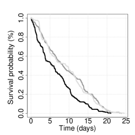
Figure 1: Kaplan-Meier survival curve, in days, for individuals fed on a) ST0 (black), b) ST1 (dark gray), and c) ST3 (gray).

Figure 1 shows a Kaplan-Meier curve, in days, for each of the ST populations considered. Individuals fed on ST0 (the control group) showed a survival curve that was lower over time in relation to the ones fed on ST1 and ST3, with a median survival time of $5.58$ days versus $8.40$ and $9.24$, respectively. The ST1 and ST3 groups exhibit similar trajectories which cross at certain time points, thus confirming a similar behaviour.

FIGURE 1 AROUND HERE

Virulence for the $i$-th worm was modelled by means of the Cox proportional hazards model

$$h_{i}(t\mid h_{0},\boldsymbol{x}_{i},\boldsymbol{\beta}) =h_{0}(t)\,\mbox{exp}\{\beta_{\texttt{1}}\,I_{\texttt{1}}(i)+\beta_{\texttt{3}}\,I_{\texttt{3}}(i)\},$$ (18)

where $I_{\texttt{1}}(i)$ and $I_{\texttt{3}}(i)$ are indicator variables for groups ST1 and ST3, respectively. It is important to highlight that $h_{i}(t\mid\cdot)=h_{0}(t)$ in the case of ST0, which acts as the control group, $h_{i}(t\mid\cdot)=h_{0}(t)\,\mbox{exp}\{\beta_{\texttt{1}}\,I_{\texttt{1}}(i)\}$ when it is ST1, and $h_{i}(t\mid\cdot)=h_{0}(t)\,\mbox{exp}\{\beta_{\texttt{3}}\,I_{\texttt{3}}(i)\}$ when the group is ST3.

We considered a Weibull model for $h_{0}(t)$ as well as $PC$ and $PS$ baseline hazard functions based on four different partitions of the time axis with number of knots $K$ = 5, 10, 25 and 40. All these partitions were chosen following the proposal by Murray et al. (2016) based on selecting intervals with the same length. The last knot in all $PC$ and $PS$ models is $24\mbox{.}50$ days, which was the longest survival time observed.

3.2 Posterior inferences

We carried out all Bayesian survival inferential processes derived from the combination of the generic specifications of the baseline hazard function above with the different prior scenarios and number of knots ($K$ = 5, 10, 25 and 40) for $PC$ and $PS$ models. The joint posterior distribution for each model was approximated using the JAGS software (Plummer, 2003). For each estimated model, we ran three parallel chains with 50,000 iterations and a burn-in of 5,000. Chains were also thinned by storing every 5th iteration to reduce autocorrelation in the sample. Convergence to the joint posterior distribution was guaranteed with a potential scale reduction factor close to 1 and an effective number of independent simulation draws greater than 100.

3.3 Model selection, hazard ratios and baseline hazard-survival function

Deviance information criterion (DIC) (Spiegelhalter et al., 2002) and log pseudo-marginal likelihood (LPML) (Geisser and Eddy, 1979) were considered for model selection. DIC measures the information on a model by means of its deviance penalized with regard to its complexity. Additionally, from the DIC computation we derived the effective number of parameters (pD) to evaluate the model complexity (Spiegelhalter et al., 2002). LPML is based on predictive criteria. It combines, on a logarithmic scale, the conditional predictive ordinate value (CPO) associated with observations of each individual (Gelfand, 1996). Smaller values for DIC are preferred, while larger LPML values indicate better predictive performance. pD is interpreted together with DIC, as a complementary criterion.

As a rule of thumb, if two models differ in the DIC by more than 3, the one with the smaller DIC is preferred as the best fitting (Spiegelhalter et al., 2002). In the case of LPML, there is no rule of thumb about how much this difference should be (Bogaerts et al., 2017). However, the LPML statistics from two competing models, $\mbox{LPML}_{1}$ and $\mbox{LPML}_{2}$, can be used to compute what has been termed a “pseudo Bayes factor” (PBF), which roughly indicates which model is superior at predicting the observed data: $\mbox{PBF}_{12}\,=\,\exp(\mbox{LPML}_{1}-\mbox{LPML}_{2})$ (Hanson and Yang, 2007; Branscum and Hanson, 2008; Zhao et al., 2014). We interpret the PBF following the guidelines proposed by Jeffreys (1961) and Kass and Raftery (1995); thus, a $\mbox{PBF}_{12}$ above 3 denotes there is substantial evidence in favour of model 1.

Table 1 shows the DIC, the pD and LPML values of the estimated models. Based on the DIC and LPML values, PS models exhibit better behaviour than Weibull or PC specifications. The Weibull model shows the worst preformance even if showing the lowest complexity (as measured by pD value). An increase in the number of knots for PC models generally results in a clear improvement in the modelling (from $K\,=\,5$ to $K\,=\,25$), since increasing $K$ up to 40 does not substantially improve goodness of fit while meaningfully increasing model complexity. Differences in DIC and PSB that are higher than 3 favour models with $K\,\leq\,25$. This fact is more relevant with correlated prior distributions, especially for scenario $PC4$. $PS$ (regardless of the number of knots and prior setting) are always the best models, showing no relevant differences between their DIC and LPML (PBF) values. Thus, PS models with $K=5$ show similar performance to their $K=10$, $K=25$ and $K=40$ counterparts. In relation to the pD values, the complexity of the models is clearly influenced by prior specification. $PC4$ and $PS3$ models (above all for $K$ = 25 and $K$ = 40) show a prior-induced parameter reduction (the true parameters (not considering hyperparameters) for $PC$ and $PS$ models can be estimated as $K$+2 and $K$+5, respectively); hence they show an improvement in model complexity with respect to their counterparts.

TABLE 1 AROUND HERE

Below we focus on the posterior stability of the posterior distribution for the hazard ratios as well as the behaviour of the subsequent marginal posterior distribution for the baseline hazard function, which reflects the natural course of the infection, and the survival function.

Hazard ratios

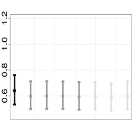
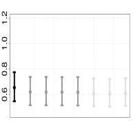
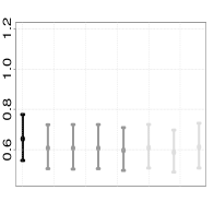
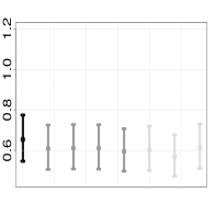
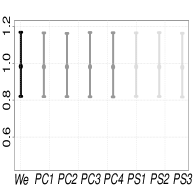
(a) K=5

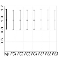
(b) K=10

(c) K=25

(d) K=40

Figure 2: Posterior mean and 95% credible interval for the hazard ratios, HR_ST1 (row one), HR_ST3 (row two) and HR_ST1/ST3 (row three), for all survival models under evaluation.

Discrepancies between the posterior marginal distributions for the regression coefficients and for any of their corresponding derived quantities, such as hazard ratios, are a result of the different modelling of $h_{0}(t)$. Figure 2 shows the posterior mean and a 95% credible interval for the hazard ratios of interest HR_ST1, HR_ST3, HR_ST1/ST3 (computed as $\pi(\exp(\beta_{1})\mid\mathcal{D})$, $\pi(\exp(\beta_{3})\mid\mathcal{D})$ and $\pi(\exp(\beta_{1}-\beta_{3})\mid\mathcal{D})$) with regard to the different specifications of the baseline hazard function, prior scenarios and number of knots for PC and PS models. HR_ST1 and HR_ST3 posterior distributions behave in a similar way, with values below 0 indicating efficacy in bacterium virulence reduction. HR_ST1/ST3 posterior distributions are centred at approximately 1, pointing to similar efficacy for both treatments. We observe great internal robustness in the results of the $PS$ models and the $PC$ models. Weibull estimated coefficients are also quite similar to those obtained from $PC$ and $PS$ models.

FIGURE 2 AROUND HERE

Baseline hazard and baseline survival functions

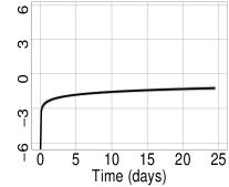
(a) We

(b) PC1

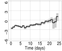
(c) PC2

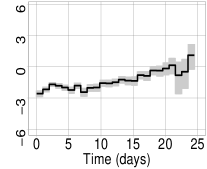
(d) PC3

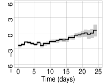
(e) PC4

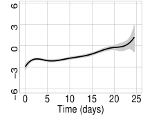
(f) PS1

(g) PS2

(h) PS3

Figure 3: Posterior mean and 95% credible interval for the log baseline hazard function under Weibull (row one), $PC$ (row two) and $PS$ (row three) scenarios. $PC$ and $PS$ models are estimated with $K=25$ and $K=5$ knots, respectively.

We now discuss the posterior distribution for $h_{0}(t)$ and the survival function of the different models in the study. Models with $K=25$ knots were selected for $PC$ specification given that the $PC4$ $(K=25)$ showed the best performance based on DIC and LPML. For $PS$ specification, $PS1$ under $K=40$ showed the best performance based on DIC, but it was dismissed since it presented clear signs of overfitting and instability in the baseline hazard value associated to the last interval. Thus, models under $K=5$ were selected because the $PS1$ was the best model according to the two selection scores and it also shows similar values of pD to those of its counterparts ($PS2$ and $PS3$ under $K=5$). Figures 3 and  4 are a matrix of graphs for illustrating baseline hazard (logarithmic scale) and survival functions posterior distributions under $We$ (row one), PC $(K=25)$ (row two) and $PS(K=5)$ (row three) models.

Baseline hazard estimates are sensitive to their specification and their implicit regularization. The $We$ model displays an increasing monotone behaviour. PC models report a general increasing trend with different ups and downs. They show wider credible intervals in regions with very little data. The $PC4$ model evidences that Bayesian regularization not only smooths the posterior mean but also reduces the uncertainty of the estimate. PS models present a more flexible baseline hazard than $PC$’s and a regularization effect is mainly observed only in uncertainty estimates. On the contrary, estimates of posterior distribution $\pi(S_{0}(t)\mid\mathcal{D})$, which is encapsulated in the unit interval, are robust to baseline hazard function specification and differences between the different modelling proposals are imperceptible.

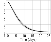
(a) We

(b) PC1

(c) PC2

(d) PC3

(e) PC4

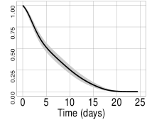
(f) PS1

(g) PS2

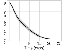
(h) PS3

Figure 4: Posterior mean and 95% credible interval for the baseline survival function under Weibull (row one), $PC$ (row two) and $PS$ (row three) scenarios. $PC$ and $PS$ models are estimated with $K=25$ and $K=5$ knots, respectively.

FIGURES 3 AND 4 AROUND HERE

3.4 Frequentist and Bayesian Cox model

Although it is not a main objective of the article, we have performed a comparison of Bayesian Cox models against their frequentist counterparts. The comparison considered the three generic baseline hazard specifications $We$, $PC$ and $PS$ to be baseline hazard functions based on the four different partitions of the time axis exploited earlier ($K$ = 5, 10, 25, and 40). For the $PC$ and $PS$ models, we only considered models $PC1$ and $PS1$ due to their “non-informative” nature in prior specification. Frequentist Cox with Weibull baseline hazard was estimated through the survreg function of the survival library. Results for the Cox $PC$ and $PS$ models were obtained by the mexhaz function of the mexhaz library, which uses the equivalence between $PC$ models and Poisson regression models (Holford, 1980; Laird and Olivier, 1981).

TABLE 2 AROUND HERE

Table 2 refers to the estimation of the hazard ratios HR_ST1 and HR_ST3. Bayesian reasoning provides the corresponding posterior mean and 95$\%$ credible interval. Frequentist statistics includes maximum likelihood estimates and 95% confidence intervals. Both estimation procedures are very stable, with similar results for $PC$ and $PS$ models.

4 Simulation study

We continue with the exploration of the impact of the baseline hazard specification in the whole inferential process, specifically the posterior estimates of the regression coefficients as well as the posterior for the hazard and survival function. We conduct three simulation studies (based on three different $h_{0}(t)$ definitions) to assess the performance of the Weibull, PC and PS definitions. $PC$ and $PS$ are also discussed with regard to different partitions of the time axis.

4.1 Simulation scenarios

Three simulation scenarios were generated from a CPH model with different specifications for $h_{0}(t)$ as described below.

Scenario 1. A Weibull distribution with an increasing hazard function ($\alpha=1.5$ and $\lambda=0.5$).
Scenario 2. A mixture of five piecewise functions

$$h_{0}(t\mid\boldsymbol{\varphi})=\sum_{k=1}^{5}\,\varphi_{k}\,I_{(c_{k-1},c_{k}]}(t),\,\,t>0,$$

where $\varphi_{1}=0.5$ in $0<t\leq 0.2$, $\varphi_{2}=2.5$ in $0.2<t\leq 0.4$, $\varphi_{3}=0.5$ in $0.4<t\leq 0.6$, $\varphi_{4}=1$ in $0.6<t\leq 0.8$, and $\varphi_{5}=1.5$ in $t>0.8$.
Scenario 3. A mixture of two Weibull distributions

$$h_{0}(t\mid\alpha_{1},\alpha_{2},\lambda_{1},\lambda_{2})=\dfrac{\lambda_{1}\,\alpha_{1}\,t^{\alpha_{1}-1}\,p\,\mbox{exp}\{-\lambda_{1}\,t^{\alpha_{1}}\}+\lambda_{2}\,\alpha_{2}\,t^{\alpha_{2}-1}\,(1-p)\,\mbox{exp}\{-\lambda_{2}\,t^{\alpha_{2}}\}}{p\,\mbox{exp}\{-\lambda_{1}\,t^{\alpha_{1}}\}+(1-p)\,\mbox{exp}\{-\lambda_{2}\,t^{\alpha_{2}}\}},\,\,t>0$$

with shape $\alpha_{1}=3$, $\alpha_{2}=1$, scale $\lambda_{1}=\lambda_{2}=0.5$, and mixing probability parameter $p=0.2$.

These scenarios included an indicator covariate with regression coefficient $\beta=1$. Data were assigned to each group according to a Bernoulli distribution with probability 0.5. We considered right censoring at time $C_{R}$. It was previously fixed for each scenario from the condition $S_{0}(C_{R})=0.3$ for the baseline survival function. Each scenario was replicated $R=100$ times for sample sizes of $N=100$ and $N=300$.

All the simulated dataset were analysed via each of the stated modellings discussed in Section 2. The estimation of the PC and PS models was based on two different partitions of the time axis with $K$ = 5 and 15 knots with intervals of the same length ((Murray et al., 2016)). The last knot in all models corresponds to the previously referred censored time ($C_{R}$), which is the longest survival time observed.

4.2 Generating survival times

We follow the inversion method (Bender et al., 2005; Austin, 2012; Crowther and Lambert, 2013) to simulate survival data for Scenarios 1 and 2. This method is based on the relationship between the cumulative distribution function (CDF) of a survival random variable and a standard uniform random variable. It can be directly applied when the subsequent CDF has a closed form expression and can be directly inverted and easily implemented with R (R Core Team, 2013) packages simsurv (Brilleman, 2013) and SimSCRPiecewise (Chapple, 2016). The inversion method for Scenario 3 is not directly suitable. The subsequent cumulative hazard function cannot be directly inverted and we have used iterative root-finding techniques (Crowther and Lambert, 2013) to solve it. This procedure is implemented for the R software (R Core Team, 2013) in the simsurv (Brilleman, 2013) package. Further details of the inversion method and its corresponding extension to simulate complex baseline hazard functions are described in the supporting information.

4.3 Posterior inferences

Each simulation dataset was used to estimate all the survival models with all the specifications of $h_{0}(t)$ and the different prior scenarios in Section 2. Posterior distributions were approximated by JAGS software (Plummer, 2003) based on three parallel chains with 20,000 iterations each plus another 2,000 for the burn-in period. Moreover, the chains were additionally thinned by storing every 10th draw to reduce autocorrelation in the sequences. Convergence of the chains to the posterior distribution was guaranteed by monitoring in all inferences to ensure that the potential scale reduction factor was close to 1 and the effective number of independent simulation draws was greater than 100.

4.4 Regression coefficients and baseline hazard function

We considered $R=100$ replicas of each inferential process and, consequently, we constructed 100 approximate random samples of the posterior distribution for $\beta$. Let $\{\beta^{(1)}_{(r)},\ldots,\beta^{(N)}_{(r)}\}$ be the approximate MCMC sample of size $N$ of the posterior marginal distribution for $\beta$ corresponding to the replica $r$.

The stability of the posterior distribution for the regression coefficients were assessed by means of the following measures:

• Bias: Difference between the average of the posterior sample means of the replicas and the true regression coefficient, $(\sum_{r=1}^{R}\,\bar{\beta}_{(r)}/R)-\beta$, where $\bar{\beta}_{(r)}$ is the sample mean of the posterior sample corresponding to the replica $r$.

• Standard error (SE): Square root $\sqrt{\sum_{r=1}^{R}\,s_{(r)}^{2}/R}$ of the average of the posterior variances $s_{(r)}^{2}$ of the replicas.

• Standard deviation (SD): Standard deviation of the set $\{\bar{\beta}_{(1)},\ldots,\bar{\beta}_{(R)}\}$ that includes the posterior sample mean of the regression coefficient of all replicas.

• Coverage probability (CP): Proportion of the $R=100$ 95$\%$ credible intervals which contain the true value of the regression coefficient.

The performance of the set of models considered was also evaluated in terms of the posterior baseline hazard estimates (logarithmic transformation). For the posterior sample of each replica we construct an approximate posterior sample of the log baseline hazard function at each time, whose average can be used as a point estimate of the true baseline hazard at that time. We then merge the information of all the replicas to obtain a global estimation, log$(\widehat{h}_{0}(t))$, by calculating their average. This procedure is also useful for extracting information about the posterior variability and constructing, for example, 95$\%$ credible intervals for the posterior of the baseline hazard at each time.

The accuracy of the estimation was measured through the difference between the posterior estimation of the baseline hazard and the true hazard function. A general measure that accounts for this difference over the time period of the study is the root-mean squared deviation (RMSD), computed as

$$\mbox{RMSD}\,=\,\sqrt{\dfrac{\sum_{m=1}^{M}[\mbox{log}(\widehat{h}_{0}(t_{m}))-\mbox{log}(h_{0}(t_{m}))]^{2}}{M}},$$ (19)

a discrete approximation based on the idea of the Riemann sums to approach an integral. At this point, we would like to note that we have used a wide partition of the time axis, with knots spaced at $0.01$ time points from 0 to the maximum time value of each scenario. This maximum time value is determined by the corresponding censoring time ($C_{R}$).

TABLES 3, 4, 5 AROUND HERE

Tables 3, 4 and 5 display the values of the average, bias, SE, SD and CP (related to $\beta$ and RMSD (related to log($h_{0}(t)$)) referring to the three simulation scenarios. In relation to the $\beta$ estimate, the $We$ model is very stable for the three scenarios and the effect of $N$ is not appreciated. $PC$ and $PS$ models approximate the regression coefficient quite well, which is slightly affected by the number of knots ($K$) and the sample size ($N$).

Under Scenario 1, the $We$ models provide the closest fit to the true function with the lowest RMSD values. PS models are generally better than PC’s, which show the worst performance, possibly because of their non-continuous behaviour. Under Scenario 2, $PC4$ models (for $N=100$ and $N=300$) provide the closest fit to the true function with the lowest RMSD values, thereby underlining the relevance of sensitivity to prior scenarios. PS models also seem to capture the behaviour of the true function, on the whole, showing RMSD values lower than the PC1, PC2, PC3 models. The $We$ models present the highest RMSD. Under Scenario 3, $PS$ models provide the lowest RMSD values as a general rule. PS3 specification shows the lowest values for all $K$ configurations. The $We$ models present higher RMSD estimates in relation to $PS$’s. Between PC’s, $PC4$ specification improves the RMSD values of its $PC$ counterparts. For all scenarios, the prior distribution has a strong effect on the baseline hazard estimation of PC models.

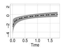
(a) We. RMSD=0.039

(b) $PC1$ ($K=5$). RMSD=0.205

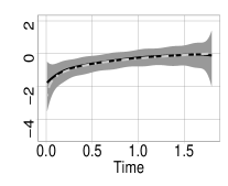
(c) PS2($K=5$). RMSD=0.095

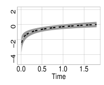
(d) We. RMSD=0.007

(e) PC3 ($K=15$). RMSD=0.130

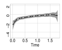
(f) PS1($K=5$). RMSD=0.063

Figure 5: Average replica pointwise of the posterior approximate means of the log-baseline hazard estimate (black solid line), average replica of the posterior 95% credible intervals (dark grey area), and true log-baseline hazard function (grey dash-dotted line) in the simulated Scenario 1 under the $We$, $PC1$ ($K=5$), $PS2$ ($K=5$) for $N$=100 (row 1) and under the $We$, $PC3$ ($K=15$), $PS1$ ($K=5$) for $N$ = 300 (row 2).

Figures 5,  6 and  7 show the posterior mean of the baseline hazard function and a 95% credible bound for the best models (based on RMSD criterion) between the three generic $h_{0}(t)$ specifications and for both $N$ values for Scenario 1, Scenario 2 and Scenario 3. In general, models under $N$ = 300 present lower RMSD values than their $N$ = 100 counterparts as well as more accurate baseline hazard estimates (95% of credible bounds are narrower).

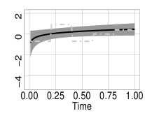
(a) We. RMSD=0.626

(b) PC4 ($K=5$). RMSD=0.095

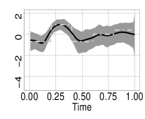
(c) PS2($K=15$). RMSD=0.289

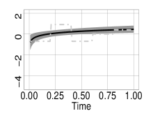
(d) We. RMSD=0.626

(e) PC3 ($K=5$). RMSD=0.042

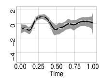
(f) PS2($K=15$). RMSD=0.254

Figure 6: Average replica pointwise of the posterior approximate means of the log-baseline hazard estimate (black solid line), average replica of the posterior 95% credible intervals (grey area), and true log-baseline hazard function (grey dash-dotted line) in the simulated Scenario 2 under the $We$, $PC4$ ($K=5$), $PS2$ ($K=15$) for $N$ = 100 (row 1) and under the $We$, $PC3$ ($K=5$), $PS2$ ($K=15$) for $N$ = 300 (row 2).

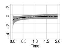
(a) We. RMSD=0.131

(b) PC4 ($K=5$). RMSD=0.116

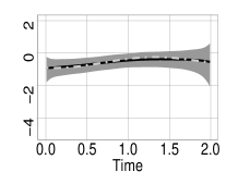
(c) PS3($K=5$). RMSD=0.074

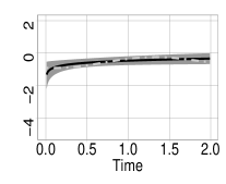
(d) We. RMSD=0.132

(e) PC1 ($K=5$). RMSD=0.066

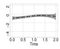
(f) PS3($K=5$). RMSD=0.043

Figure 7: Average replica pointwise of the posterior approximate means of the log-baseline hazard estimate (black solid line), average replica of the posterior 95% credible intervals (grey area), and true log-baseline hazard function (grey dash-dotted line) in the simulated Scenario 3 under the $We$, $PC4$ ($K=5$), $PS3$ ($K=5$) for $N$ = 100 (row 1) and under the $We$, $PC1$ ($K=5$), $PS3$ ($K=5$) for $N$ = 300 (row 3).

FIGURES 5, 6, 7 AROUND HERE

5 Conclusions

We have discussed different proposals for performing a fully time-to-event Bayesian analysis in the context of the CPH model via parametric and semi-parametric definitions of the baseline hazard function. The Bayesian methodology allows the baseline hazard functions to be implemented in an easy conceptual way, even semi-parametric proposals that are necessary in contexts in which a certain complexity in the shape of the underlying function is expected. On this matter, we have examined some of the most popular proposals in the literature related to the subject: the Weibull distribution as the most common parametric model, and piecewise constant and cubic B-spline baseline hazards as semi-parametric definitions. Flexibility and overfitting were discussed within both semi-parametric options with regard to different regularization schemes expressed in terms of prior distributions and time axis partition configurations. These developments provide a unified framework to conduct a fully Bayesian analysis of complex survival data that will surely encourage more comprehensive analyses, which currently often rely on some versions of the CPH model without further examination. The flexibility of our approach allows for easy subsequent research on prior sensitivity, different criteria for determining the axis partition of non-parametric proposals and relationships between covariates and baseline hazard functions. Additionally, we have also incorporated a comparison with the frequentist approach to evaluate the performance of both methodologies under the CPH model.

The virulence database in Section 3 illustrates the main goals of this paper. All inferential processes agree with the conclusions in Sanz-Puig et al. (2017) that the cauliflower by-product infusion can be an alternative preservation treatment. This fact evidences the robustness (regardless of the $h_{0}(t)$ specification) of the Cox model in estimating covariate effects. However, $PC$ models show a certain sensitivity to axis partition in estimating covariate effects. The outcomes also highlight the fact that piecewise constant and B-splines specifications allow us to capture and introduce (dealing with different axis partition configurations) more flexibility in $h_{0}(t)$. However, piecewise constant options exhibit less flexibility, thus requiring a higher number of $K$ as well as a prior correlation specification to behave in a similar way to B-splines. Hence, in this illustrative example the $PC$ model underlines the efficacy of regularization Bayesian methods (based on defining correlation by means of prior definition) to overcome overfitting and instability in baseline hazard estimation under high $K$ values. In relation to the survival function estimation, this derived quantity shows greater robustness regardless of the baseline hazard specification. Both DIC and LPML reinforce the evidence observed in sensitivity analyses in which PS models show better behaviour than $PC$ models irrespective of the number of pre-fixed knots. Frequentist methods showed similar performance to the Bayesian in the Cox inferential process within a framework of non-regularization in relation to Weibull and B-spline specification.
We have also exemplified our proposals through different simulated data generated by Weibull, piecewise constant and mixtures of Weibull baseline hazard functions. In general, the outcomes indicate that moderate bias can be observed in estimates of the regression coefficient for a treatment effect when the baseline hazard function specification does not match the origin specification. For baseline hazard estimates, we appreciate small differences between the true baseline hazard and their point estimates, and lower RMSD values have a close relationship with the data-generating model. In terms of RMSD estimates the Weibull model provides the best results with Weibull simulated data, although $PS$ models also exhibit good behaviour. In the case of piecewise constant simulated data, the PC4 model is the best model, although PS models present a very good behaviour in terms of RMSD values. PS3 models provide the best estimates for the Weibull mixture data. In relation to the performance of the different number of knot configurations ($K$) explored, it is generally noticeable that PC models require a higher number of $K$ than $PS$ models within the same scenario. Thus, the need for regularization becomes more evident under $PC$ models. In all scenarios, the impact of the database size has generally been evident mainly in the estimation of the baseline hazard function, but has been less evident in the regression coefficient estimate.
Although in this article we have extolled the potential of Bayesian inference in dealing with semi-parametric specifications for the baseline hazard in the context of the CPH model, it must be stated that in many settings a simpler distribution may be suitable. However, using a more complex distribution can provide far more realistic inferences in certain situations. Some interesting issues that are beyond the scope of this paper deal with introducing uncertainty in the number of knots, including new regularization proposals such as penalized complexity priors, carrying out a sensitivity analysis within each scenario and also exploring in greater depth the performance of the frequentist approach under the “semi-parametric” specification of the baseline hazard function.

Model	$\boldsymbol{K}$	DIC	pD	LPML	Model	$\boldsymbol{K}$	DIC	pD	LPML
$We$	-	4553.309	3.960	-2276.334
$PC1$	5	4484.455	7.030	-2241.921	$PS1$	5	4460.598	9.930	-2230.660
	10	4478.040	12.067	-2238.658		10	4462.866	14.368	-2231.988
	25	4469.406	27.313	-2235.836		25	4462.494	29.007	-2236.958
	40	4488.393	43.036	-2249.157		40	4419.711	42.537	-2230.357
$PC2$	5	4484.457	7.030	-2241.917	$PS2$	5	4460.024	9.537	-2230.207
	10	4478.069	12.081	-2238.661		10	4462.249	13.831	-2231.412
	25	4469.371	27.295	-2236.586		25	4463.873	26.345	-2233.509
	40	4488.417	43.047	-2249.814		40	4463.732	38.084	-2235.947
$PC3$	5	4484.439	7.021	-2241.905	$PS3$	5	4459.578	8.572	-2229.787
	10	4477.979	12.036	-2238.632		10	4458.998	10.467	-2229.443
	25	4469.221	27.219	-2235.719		25	4460.255	13.471	-2230.112
	40	4487.049	42.356	-2245.979		40	4458.403	15.583	-2229.296
$PC4$	5	4484.445	7.014	-2241.894
	10	4477.070	11.508	-2238.193
	25	4463.265	22.566	-2231.649
	40	4471.340	29.782	-2235.798

Table 1: DIC, pD and LPML values for the survival models defined by means of Weibull, $PC$ and $PS$ specifications of the baseline hazard function with number of knots $K$ = 5, 10, 25, and 40.

		Bayesian approach		Frequentist approach
Model	$\boldsymbol{K}$	HRST1	HRST3	HRST1	HRST3
$We$	–	0.640 (0.533, 0.760)	0.654 (0.546, 0.774)	0.637 (0.534, 0.760)	0.652 (0.546, 0.777)
	5	0.604 (0.503, 0.722)	0.619 (0.515, 0.737)	0.601 (0.503, 0.719)	0.616 (0.515, 0.736)
$PC1$	10	0.598 (0.498, 0.712)	0.615 (0.513, 0.732)	0.596 (0.498, 0.713)	0.613 (0.512, 0.733)
	25	0.594 (0.495, 0.707)	0.607 (0.505, 0.723)	0.592 (0.495, 0.708)	0.605 (0.506, 0.723)
	40	0.594 (0.494, 0.708)	0.608 (0.507, 0.725)	0.593 (0.496, 0.709)	0.608 (0.508, 0.727)
$PS1$	5	0.596 (0.496, 0.709)	0.610 (0.508, 0.725)	0.593 (0.495, 0.709)	0.607 (0.508, 0.726)
	10	0.592 (0.493, 0.706)	0.605 (0.505, 0.719)	0.593 (0.495, 0.709)	0.606 (0.506, 0.725)
	25	0.592 (0.493, 0.705)	0.610 (0.509, 0.725)	0.592 (0.495, 0.709)	0.606 (0.507, 0.725)
	40	0.590 (0.491, 0.702)	0.603 (0.501, 0.719)	0.592 (0.495, 0.709)	0.606 (0.507, 0.725)

Table 2: HR_ST1 and HR_ST3: posterior mean and 95% credible interval (Bayesian approach), and estimate and 95% confidence intervals (Frequentist approach).

Model	$\boldsymbol{N}$	$\boldsymbol{K}$	$\boldsymbol{\beta}$					log$\boldsymbol{({h}_{0}(t))}$
			Average	Bias	SE	SD	CP	RMSD
$We$	100	–	1.035	0.035	0.230	0.211	0.97	0.039
	300	–	1.008	0.008	0.132	0.136	0.95	0.007
$PC1$	100	5	1.037	0.037	0.233	0.216	0.96	0.205
		15	1.049	0.049	0.234	0.216	0.97	2.158
	300	5	1.004	0.004	0.133	0.140	0.95	0.198
		15	1.013	0.013	0.133	0.142	0.95	0.131
$PC2$	100	5	1.038	0.038	0.233	0.215	0.96	0.205
		15	1.051	0.051	0.234	0.216	0.97	3.607
	300	5	1.004	0.004	0.133	0.140	0.96	0.198
		15	1.013	0.013	0.134	0.141	0.97	0.131
$PC3$	100	5	1.037	0.037	0.234	0.216	0.95	0.205
		15	1.050	0.050	0.234	0.216	0.96	1.083
	300	5	1.004	0.004	0.133	0.140	0.96	0.198
		15	1.014	0.014	0.134	0.142	0.97	0.130
$PC4$	100	5	0.946	-0.054	0.234	0.210	0.97	0.212
		15	0.882	-0.118	0.233	0.203	0.96	0.206
	300	5	0.970	-0.030	0.134	0.140	0.96	0.204
		15	0.944	-0.056	0.133	0.139	0.93	0.145
$PS1$	100	5	1.031	0.031	0.232	0.211	0.98	0.117
		15	0.996	-0.004	0.228	0.203	0.97	0.205
	300	5	1.010	0.010	0.133	0.140	0.95	0.063
		15	0.994	-0.006	0.132	0.137	0.96	0.120
$PS2$	100	5	0.925	-0.075	0.231	0.205	0.96	0.095
		15	0.788	-0.212	0.225	0.189	0.88	0.201
	300	5	0.967	-0.033	0.133	0.139	0.95	0.064
		15	0.902	-0.098	0.131	0.134	0.86	0.116
$PS3$	100	5	1.027	0.027	0.233	0.210	0.97	0.096
		15	1.023	0.023	0.234	0.209	0.97	0.121
	300	5	1.007	0.007	0.134	0.140	0.97	0.071
		15	1.005	0.005	0.134	0.140	0.97	0.089

Table 3: Average, bias, SE, SD and CP of the regression coefficient $\beta$ and RMSD of the log$({h}_{0}(t))$ corresponding to all inferential and replicate processes for the Scenario 1 simulated data.

Model	$\boldsymbol{N}$	$\boldsymbol{K}$	$\boldsymbol{\beta}$					log$\boldsymbol{({h}_{0}(t))}$
			Average	Bias	SE	SD	CP	RMSD
$We$	100	–	1.077	0.077	0.234	0.251	0.93	0.626
	300	–	1.074	0.074	0.133	0.163	0.88	0.626
$PC1$	100	5	1.018	0.018	0.234	0.232	0.94	0.276
		15	1.018	0.018	0.235	0.229	0.95	7.933
	300	5	1.012	0.012	0.133	0.149	0.95	0.058
		15	1.013	0.013	0.134	0.150	0.92	0.889
$PC2$	100	5	1.018	0.018	0.234	0.232	0.94	0.760
		15	1.017	0.017	0.235	0.229	0.95	13.085
	300	5	1.011	0.011	0.133	0.149	0.94	0.058
		15	1.013	0.013	0.134	0.151	0.92	1.291
$PC3$	100	5	1.017	0.017	0.233	0.232	0.94	0.345
		15	1.017	0.017	0.235	0.229	0.95	4.381
	300	5	1.012	0.012	0.134	0.149	0.94	0.058
		15	1.013	0.013	0.134	0.150	0.92	0.276
$PC4$	100	5	1.001	0.001	0.230	0.226	0.94	0.095
		15	0.973	-0.027	0.228	0.216	0.95	0.202
	300	5	1.006	0.006	0.133	0.148	0.94	0.042
		15	0.996	-0.004	0.133	0.147	0.92	0.102
$PS1$	100	5	1.012	0.012	0.233	0.225	0.94	0.421
		15	0.992	-0.008	0.231	0.223	0.95	0.402
	300	5	1.013	0.013	0.134	0.150	0.92	0.387
		15	1.003	0.003	0.133	0.147	0.94	0.303
$PS2$	100	5	1.001	0.001	0.226	0.211	0.96	0.405
		15	0.975	-0.025	0.214	0.190	0.97	0.289
	300	5	1.008	0.008	0.132	0.147	0.92	0.386
		15	0.993	-0.007	0.128	0.137	0.94	0.254
$PS3$	100	5	1.018	0.018	0.234	0.229	0.94	0.424
		15	1.015	0.015	0.235	0.229	0.94	0.305
	300	5	1.014	0.014	0.134	0.151	0.92	0.388
		15	1.012	0.012	0.134	0.150	0.92	0.261

Table 4: Average, bias, SE, SD and CP of the regression coefficient $\beta$ and RMSD of the log$({h}_{0}(t))$ corresponding to all inferential and replicate processes for the Scenario 2 simulated data.

Model	$\boldsymbol{N}$	$\boldsymbol{K}$	$\boldsymbol{\beta}$					log$\boldsymbol{({h}_{0}(t))}$
			Average	Bias	SE	SD	CP	RMSD
$We$	100	–	0.955	-0.045	0.230	0.234	0.93	0.131
	300	–	0.960	-0.040	0.131	0.119	0.94	0.132
$PC1$	100	5	0.983	-0.017	0.234	0.254	0.93	0.309
		15	0.989	-0.011	0.235	0.254	0.93	4.524
	300	5	0.979	-0.021	0.133	0.120	0.95	0.066
		15	0.984	-0.016	0.133	0.121	0.95	0.245
$PC2$	100	5	0.985	-0.015	0.234	0.255	0.93	0.831
		15	0.992	-0.008	0.235	0.255	0.93	7.012
	300	5	0.980	-0.020	0.133	0.121	0.95	0.066
		15	0.984	-0.016	0.133	0.122	0.96	0.313
$PC3$	100	5	0.984	-0.016	0.234	0.254	0.93	0.466
		15	0.991	-0.009	0.235	0.255	0.94	3.962
	300	5	0.979	-0.021	0.133	0.120	0.95	0.066
		15	0.984	-0.016	0.133	0.122	0.96	0.102
$PC4$	100	5	0.865	-0.135	0.236	0.251	0.88	0.116
		15	0.802	-0.198	0.232	0.240	0.83	0.141
	300	5	0.938	-0.062	0.133	0.121	0.94	0.077
		15	0.902	-0.098	0.133	0.118	0.91	0.075
$PS1$	100	5	0.978	-0.022	0.232	0.251	0.93	0.136
		15	0.941	-0.059	0.228	0.243	0.93	0.224
	300	5	0.980	-0.020	0.133	0.121	0.96	0.053
		15	0.967	-0.033	0.132	0.121	0.94	0.129
$PS2$	100	5	0.822	-0.178	0.233	0.252	0.84	0.127
		15	0.675	-0.325	0.223	0.236	0.71	0.235
	300	5	0.917	-0.083	0.133	0.123	0.91	0.058
		15	0.844	-0.156	0.132	0.122	0.80	0.114
$PS3$	100	5	0.966	-0.034	0.233	0.244	0.92	0.074
		15	0.964	-0.036	0.233	0.242	0.92	0.084
	300	5	0.974	-0.026	0.133	0.120	0.95	0.043
		15	0.973	-0.027	0.133	0.119	0.95	0.048

Table 5: Average, bias, SE, SD and CP of the regression coefficient $\beta$ and RMSD of the log$({h}_{0}(t))$ corresponding to all inferential and replicate processes for the Scenario 3 simulated data.

Lázaro’s work was supported by a predoctoral FPU fellowship (FPU2013/02042) from the Spanish Ministry of Education, Culture and Sports. This research work was funded by grant MTM2016-77501-P from the Spanish Ministry of Economy and Competitiveness co-financed with FEDER funds.

Conflict of Interest

The authors have declared no conflict of interest.

References

- Andersen and Gill (1982) Andersen, P. K., and R. D. Gill. 1982. Cox’s regression model for counting processes: A large sample study. Annals of Statistics 10: 1100–1120.
- Austin (2012) Austin, P. C. 2012. Generating survival times to simulate Cox proportional hazards models with time-varying covariates. Statistics in Medicine 31 (29): 3946–3958.
- Banerjee et al. (2014) Banerjee, S., B. P. Carlin, and Alan E A. E. Gelfand. 2014. Hierarchical modeling and analysis for spatial data. Boca Raton, Chapman & Hall Crc Press.
- Belitz et al. (2015) Belitz, C., A. Brezger, T. Kneib, S. Lang, and N. Umlauf. 2015. Bayesx software for Bayesian inference in structured additive regression models version 2.0.1. URL http://www. bayesx. org.
- Bender et al. (2005) Bender, R., T. Augustin, and M. Blettner. 2005. Generating survival times to simulate Cox proportional hazards models. Statistics in Medicine 24 (11): 1713–1723.
- Benner et al. (1988) Benner, A., M. Zucknick, T. Hielscher, C. I., and U. Mansmann. 1988. Monotone regression splines in action. Statistical Science 3: 425–461.
- Benner et al. (2010) Benner, A., M. Zucknick, T. Hielscher, C. I., and U. Mansmann. 2010. High-dimensional cox models: the choice of penalty as part of the model building process. Biometrical Journal 52: 50–69.
- Berger et al. (1994) Berger, James, Elías Moreno, Luis Pericchi, M. Bayarri, Jose Bernardo, Juan Cano, Julián Horra, Jacinto Martín, David Rios, Bruno Betrò, A. Dasgupta, Paul Gustafson, Larry Wasserman, Joseph Kadane, Cid Srinivasan, Michael Lavine, Anthony O’Hagan, Wolfgang Polasek, Christian Robert, and Siva Sivaganesan. 1994. An overview of robust bayesian analysis. Test 3: 5–124.
- Bernardo (1979) Bernardo, Jose M. 1979. Reference posterior distributions for Bayesian inference. Journal of the Royal Statistical Society. Series B (Methodological).
- Bickel (2006) Bickel, P. J. 2006. Regularization in statistics. Test 15: 271–344.
- Bogaerts et al. (2017) Bogaerts, K., A. Komarek, and E. Lesaffre. 2017. Survival analysis with interval-censored data: A practical approach with examples in R, SAS, and BUGS. Chapman and Hall/CRC.
- Boor (1978) Boor, C. De. 1978. A practical guide to splines. New York, Springer-Verlag.
- Branscum and Hanson (2008) Branscum, A., and T. E. Hanson. 2008. Bayesian nonparametric meta-analysis using Polya tree mixture models. Biometrics 64 (3): 825–833.
- Breiman (1996) Breiman, L. 1996. Bagging predictors. Machine Learning 24 (2): 123–140.
- Breslow (1974) Breslow, N. 1974. Covariance analysis of censored survival data. Biometrics 30 (1): 89–99.
- Brilleman (2013) Brilleman, S. 2013. simsurv: Simulate Survival Data. R package version 0.1.0.
- Cai et al. (2002) Cai, T., R. J. Hyndman, and M. P. Wand. 2002. Mixed model-based hazard estimation. Journal of Computational and Graphical Statistics 11 (4): 784–798.
- Chapple (2016) Chapple, A. G. 2016. SimSCRPiecewise: Simulates Univariate and Semi-Competing Risks Data Given Covariates and Piecewise Exponential Baseline Hazards. R package version 0.1.1.
- Christensen et al. (2011) Christensen, R., J. Wesley, A. Branscum, and T. E. Hanson. 2011. Bayesian Ideas and Data Analysis: An Introduction for Scientists and Statisticians. Boca Raton, Chapman & Hall/CRC Press.
- Cox (1972) Cox, D. 1972. Regression models and life tables (with discussion). Journal of the Royal Statistical Society 34: 187–220.
- Crainiceanu et al. (2005) Crainiceanu, C. M., D. Ruppert, and M. P. Wand. 2005. Bayesian Analysis for Penalized Spline Regression Using WinBUGS. Journal of Statistical Software 14 (14): 1–24.
- Crowther and Lambert (2013) Crowther, M. J., and P. C. Lambert. 2013. Simulating biologically plausible complex survival data. Statistics in Medicine 32 (23): 4118–4134.
- Dellaportas and Smith (1993) Dellaportas, P., and A. F. M. Smith. 1993. Bayesian inference for generalized linear and proportional hazards models via Gibbs sampling. Applied Statistics.
- Fahrmeir and Hennerfeind (2003) Fahrmeir, L., and A. Hennerfeind. 2003. Nonparametric Bayesian hazard rate models based on penalized splines, Technical report, Discussion paper//Sonderforschungsbereich 386 der Ludwig-Maximilians-Universität München.
- Fahrmeir and Kneib (2011) Fahrmeir, L., and T. Kneib. 2011. Bayesian smoothing and regression for longitudinal, spatial and event history data. Oxford, Oxford University Press.
- Geisser and Eddy (1979) Geisser, S., and W. F. Eddy. 1979. A predictive approach to model selection. Journal of the American Statistical Association 74 (365): 153–160.
- Gelfand (1996) Gelfand, A. E. 1996. Markov chain monte carlo in practice, 146–151. London, Chapman & Hall/CRC Press.
- Gelman (2006) Gelman, A. 2006. Prior distributions for variance parameters in hierarchical models (comment on article by Browne and Draper). Bayesian Analysis 1 (3): 515–534.
- Girosi et al. (1993) Girosi, F., M. Jones, T. Poggio, J. A. Doornik, and H. Hansen. 1993. Priors stabilizers and basis functions: From regularization to radial, tensor and additive splines, C. b. c. l. paper no. 75, Artificial Intelligence Laboratory Massachusetts Institute of Technology.
- Hanson and Yang (2007) Hanson, T., and M. Yang. 2007. Bayesian semiparametric proportional odds models. Biometrics 63 (1): 88–95.
- Hastie et al. (2009) Hastie, T., R. Tibshirani, and J. Friedman. 2009. The Elements of Statistical Learning. New York, Springer-Verlag.
- Henschel et al. (2009) Henschel, V., J. Engel, D. Hölzel, and U. Mansmann. 2009. A semiparametric Bayesian proportional hazards model for interval censored data with frailty effects. BMC Medical Research Methodology 9 (1): 9.
- Holford (1980) Holford, Theodore R. 1980. The analysis of rates and of survivorship using log-linear models. Biometrics 36 (2): 299–305.
- Ibrahim et al. (2001) Ibrahim, J. G., M. H. Chen, and D. Sinha. 2001. Bayesian survival analysis. New York, Springer-Verlag.
- Ibrahim et al. (2011) Ibrahim, J. G., H. Zhu, and N. Tang. 2011. Bayesian local influence for survival models. Lifetime Data Analysis 17 (1): 43–70.
- Jeffreys (1961) Jeffreys, H. 1961. The theory of probability. Oxford University Press.
- Kalbfleisch and Prentice (1973) Kalbfleisch, J. D., and R. L. Prentice. 1973. Marginal likelihoods based on Cox’s regression and life model. Biometrika 60 (2): 267–278.
- Kass and Raftery (1995) Kass, R. E., and A. E. Raftery. 1995. Bayes factors. Journal of the American Statistical Association 90 (430): 773–795.
- Kim and Ibrahim (2000) Kim, S. W., and J. G. Ibrahim. 2000. On Bayesian inference for proportional hazards models using noninformative priors. Lifetime Data Analysis 6 (4): 331–341.
- Laird and Olivier (1981) Laird, N., and D. Olivier. 1981. Covariance analysis of censored survival data using log-linear analysis techniques. Journal of the American Statistical Association 76 (374): 231–240.
- Lang and Brezger (2004) Lang, S., and A. Brezger. 2004. Bayesian P-splines. Journal of Computational and Graphical Statistics 13 (1): 183–212.
- Lee et al. (2016) Lee, K. H., F. Dominici, D. Schrag, and S. Haneuse. 2016. Hierarchical models for semicompeting risks data with application to quality of end-of-life care for pancreatic cancer. Journal of the American Statistical Association 111 (515): 1075–1095.
- Murray et al. (2016) Murray, T. A., B. P. Hobbs, D. J. Sargent, and B. P. Carlin. 2016. Flexible Bayesian survival modeling with semiparametric time-dependent and shape-restricted covariate effects. Bayesian Analysis 11 (2): 381.
- P. H. C. Eilers and Durbán (2015) P. H. C. Eilers, B. D. Marx, and M. Durbán. 2015. Twenty years of p-splines. SORT, Statistics & Operations Research Biometrical Journal 39: 149–186.
- Plummer (2003) Plummer, M. 2003. JAGS: a program for analysis of Bayesian graphical models using Gibbs sampling. In Proceedings of the 3rd international workshop on distributed statistical computing.
- R Core Team (2013) R Core Team. 2013. R: A Language and Environment for Statistical Computing. Vienna, Austria. R Foundation for Statistical Computing. http://www.R-project.org/.
- Royston (2011) Royston, P. 2011. Estimating a smooth baseline hazard function for the Cox model. Department of Statistical Science, University College London Research report 314.
- Sahu et al. (1997) Sahu, S. K., D. K. Dey, H. Aslanidou, and D. Sinha. 1997. A Weibull regression model with gamma frailties for multivariate survival data. Lifetime Data Analysis 3 (2): 123–137.
- Sanz-Puig et al. (2017) Sanz-Puig, M., E. Lázaro, C. Armero, D. Alvares, A. Martínez, and D. Rodrigo. 2017. S. Typhimurium virulence changes caused by exposure to different non-thermal preservation treatments using C. elegans. International Journal of Food Microbiology 262: 49–54.
- Sharef et al. (2010) Sharef, E., R. L. Strawderman, D. Ruppert, M. Cowen, and L. Halasyamani. 2010. Bayesian adaptative b-spline estimationin proportional hazards frailty models. Electronic Journal of Statistics 4: 606–642.
- Sherar (2004) Sherar, P. A. 2004. Variational based analysis and modelling using B-splines. PhD diss, School of Engineering. Cranfield University.
- Spiegelhalter et al. (2002) Spiegelhalter, D. J., N. G. Best, B. P. Carlin, and A. Van Der Linde. 2002. Bayesian measures of model complexity and fit. Journal of the Royal Statistical Society: Series B (Statistical Methodology) 64 (4): 583–639.
- Tsiatis (1981) Tsiatis, A. A. 1981. A large sample study of cox’s regression model. Annals of Statistics 9: 93–108.
- van Houwelingen and Stijnen (2014) van Houwelingen, H. C., and T. Stijnen. 2014. Cox regression model. In Handbook of survival analysis, ed. Ibrahim JG Scheike TH (eds) Klein J van Houwelingen H, 5–26. Boca Raton, Chapman & Hall.
- Zhao et al. (2014) Zhao, L., D. Feng, E. L. Bellile, and J. M. G. Taylor. 2014. Bayesian random threshold estimation in a Cox proportional hazards cure model. Statistics in medicine 33 (4): 650–661.