Robust Inference for Generalized Linear Mixed Models: An Approach Based on Score Sign Flipping

Abstract

Despite the versatility of generalized linear mixed models in handling complex experimental designs, they often suffer from misspecification and convergence problems. This makes inference on the values of coefficients problematic. To address these challenges, we propose a robust extension of the score-based statistical test using sign-flipping transformations. Our approach efficiently handles within-variance structure and heteroscedasticity, ensuring accurate regression coefficient testing. The approach is illustrated by analyzing the reduction of health issues over time for newly adopted children. The model is characterized by a binomial response with unbalanced frequencies and several categorical and continuous predictors. The proposed approach efficiently deals with critical problems related to longitudinal nonlinear models, surpassing common statistical approaches such as generalized estimating equations and generalized linear mixed models.

Keywords: Generalized linear mixed model, Robustness, Score test, longitudinal data, sign flipping.

1 Introduction

Generalized linear mixed models (GLMM) play a pivotal role in psychometric data analysis due to their ability to handle clustered data structures such as longitudinal data when the response variable follows a non-normal distribution, e.g., repeated measures of a binary item across subjects (Cnaan et al.,, 1997; Tuerlinckx et al.,, 2006). Despite their popularity, important drawbacks are sensitivity to model violations and computational issues. Flexibility in dealing with a complex data structure is coupled with a strong reliance on the underlying parametric assumptions.

As a prototypical example, in this paper, we make use of the dataset on follow-up reports of Italian children adopted from foreign countries presented in Santona et al., (2022). The dataset comprises $527$ children. The follow-up questionnaires are administered to children at different times (depending on the regulations of the foreign countries) and range from $4$ to $6$ follow-ups, for a total of $3116$ observations. The health status is measured through the analysis of several questions. The research aim is to explore the adaptation of adopted children to their new family and to the social environment during the early stages of adoption, as well as how this adaptation evolves over time. In this analysis, we will focus on the presence or absence of health issues (i.e., a binary variable). The within-subject variable is then the month from the adoption, while other subject-specific socio-demographic variables (i.e. gender, age, country of origin) are also included in the model.

The fitting of a GLMM with a logistic link function and a binomial response reveals initial difficulties. One of them is that the default optimization method fails to converge, leading to unreliable model parameter estimates. Using alternative constrained optimization methods based on quadratic approximation is necessary by setting a high threshold for the number of times the function can be evaluated within the algorithm, which leads to a large increase in computational time and space complexity. In addition, the specification of the GLMM is not so straightforward. The researcher must decide which variables are considered as random effects and which type of random effect must be inserted into the model. These decisions directly impact the correctness of statistical inference on the coefficients, and the proper choice between a parsimonious model (Bates et al., 2015a, ) and a maximal model (Barr et al.,, 2013) is still an open problem.

In order to deal with these problems, this paper presents a robust approach for coping with inference on binary responses with a complex correlation structure, e.g., longitudinal data. The method can deal with any dependent variable following a generalized linear model (GLM) (Agresti,, 2015) under the usual regularity condition (Azzalini,, 2017). As pointed out at the beginning of the introduction, problems related to the popular generalized linear mixed models are numerous and are summarized below.

First, generalized linear (mixed) models are frequently misspecified due to overdispersion, heteroscedasticity, or neglecting nuisance variables. In case of misspecification, traditional parametric tests (i.e., tests that exclusively depend on an assumed parametric model to compute the null distribution of the test statistic) may lose their validity as they rely on estimating the Fisher information under incorrect assumptions (Heagerty and Kurland,, 2001). An alternative approach for testing regression coefficients in potentially misspecified GLMs is to employ a Wald-type test with a robust variance estimator (i.e., the sandwich estimator). However, for small to moderate sample sizes, sandwich estimates are rather inaccurate, leading to overly liberal tests (Hemerik et al.,, 2020). Moreover, existing quasi-likelihood methods (e.g., Generalized Estimating Equation (GEE)) for testing in misspecified models often fail to provide satisfactory control over the type I error rate as underlined by Hemerik et al., (2020). Even when well-specified, these tests control type I errors only asymptotically.

Second, the estimation process of generalized linear mixed models, having no closed-form solution for the likelihood function, can encounter convergence issues, especially in the presence of complex random effect structures. The main factors contributing to these problems include high dimensionality, non-identifiability, singular design matrices, imbalanced and sparse data, and high sensitivity to starting values, even if strong assumptions are made to simplify the estimation process. Again, these lead to invalid inferences, increased computational time, and resource use.

In summary, model misspecification and convergence issues are important concerns that can impact the reliability of inferences. The robustness of the significance tests depends not only on the degree of agreement between the specified mathematical model and the actual population data structure but also on the precision and robustness of the computational criteria for fitting the specified covariance structure to the data.

To address these challenges, nonparametric methods, such as permutation tests, prove useful for testing the effects of covariates. It is well known that permutation theory has emerged as a promising alternative to traditional, parametric statistical approaches, providing more robust and reliable inference for various hypothesis testing scenarios (Pesarin,, 2001). Kherad-Pajouh and Renaud, (2010) and Lee and Braun, (2012) proposed nonparametric tests for linear mixed models. The first one is based on permuted residuals, while the second one is based on the best linear unbiased predictors and restricted likelihood ratio test statistic. However, both rely on the Gaussian assumption distribution of the outcome. Instead, Basso and Finos, (2012); Finos and Basso, (2014) proposed a permutation test for the generalized linear mixed model based on the parametric statistical test. Basso and Finos, (2012); Finos and Basso, (2014) fit a model for each cluster/subject, and then the parameter of interest is estimated and tested considering the within-subject estimated coefficients as responses. Basso and Finos, (2012) deal with testing within-subjects effect while Finos and Basso, (2014) the between-subject one. The test proposed by Basso and Finos, (2012) is exact but has low power since the power of the statistical test depends on the quality of estimating the covariance of the cluster-level parameter estimator. In contrast, the statistical test presented by Finos and Basso, (2014) is exact only in the case of balanced number of within-subject observations. In addition, the approach of Finos and Basso, (2014) heavily relies on an adequate estimate of the Fisher Information.

This paper investigates challenges and novel methodologies for testing regression coefficients in generalized linear mixed models. We rely on the resampling-based procedure recently proposed by Hemerik et al., (2020) and De Santis et al., (2022) to solve the above-mentioned problems. We extend their approach, dealing with the within-subject dependence that characterizes longitudinal data and the heteroscedasticity between groups of observations. The test proposed by Hemerik et al., (2020) computes effective scores and randomly sign-flips each subject’s contribution to the score. The method is improved in De Santis et al., (2022) by including additional standardization steps. This leads to a test that has excellent small-sample performance and is asymptotically valid under any variance misspecification. Our method exploits the “whole-block exchangeability” concept suggested in a heuristic way by Winkler et al., (2014) for dealing with the within-variance structure of the non-normal longitudinal data. Whole-block exchangeability allows for a statistical approach based on block-wise sign-flipping. This approach was previously limited to linear mixed models, while we extend it to generalized linear mixed models. Thus, within-subject correlation is handled nonparametrically by a permutation-type method, where we use reflections, i.e., sign-flipping, rather than permutations.

The article is organized as follows. Section 2 outlines the sign-flipping test proposed by De Santis et al., (2022). This approach is extended to clustered data in Section 3. We propose a brief comparison between the GEE quasi-likelihood approach and the proposed method in Section 4. Section 5 evaluates by simulations the performance of our method in comparison with the GLM, GLMM, and GEE testing in terms of type I error control and power. Finally, Section 6 presents our case study, highlighting how, thanks to the proposed approach, it is possible to provide robust inference for binary longitudinal data.

The method proposed is efficiently implemented in the R package flipscores (Finos et al.,, 2023), which is compatible with large datasets and complex statistical models. Along the manuscript, we will therefore call the proposed method the flipscores approach.

2 Sign-flipping score test with independent observations

We introduce the method proposed by De Santis et al., (2022) for inference on regression coefficients in GLM, which improves Hemerik et al., (2020)’s approach, particularly in the case of small sample size. The statistical test is based on randomly flipping the signs of scores (i.e., one score for each subject), which is robust to misspecification of the variance in the GLM framework. The notation used throughout the manuscript follows that used by De Santis et al., (2022).

Consider $n$ independent observations $y_{1},\dots,y_{n}$ following a GLM from the exponential dispersion family (Agresti,, 2015):

$$f(y_{i};\theta_{i};\phi_{i})=\exp\Big{\{}\dfrac{y_{i}\theta_{i}-b(\theta_{i})}{a(\phi_{i})}+c(y_{i},\phi_{i})\Big{\}}$$

where $\theta_{i}$ is the canonical parameter, $\phi_{i}$ the dispersion one, and $\mu_{i}=\mathrm{E}(y_{i})=b^{\prime}(\theta_{i})$. The generalized linear model is then defined as:

$$g(\mu)=\eta=X\beta+Z\gamma$$

where $g(\cdot)$ is the link function, $\mu=(\mu_{1},\dots,\mu_{n})^{\top}$, $X$ and $Z$ are the design matrices corresponding to the parameter $\beta$ of interest and the $q$ nuisance parameters $\gamma$ respectively. The case of one parameter of interest, i.e., $\mathrm{dim}(X)=n\times 1$, is then considered. However, the approach is extendable to the multivariate case (Hemerik et al.,, 2020; De Santis et al.,, 2022).

The main focus is to test the null hypothesis $H_{0}:\beta=\beta_{0}\mid\gamma,\phi_{1},\dots,\phi_{n}$. The test statistic used in Hemerik et al., (2020) is the effective score:

$$S=n^{-1/2}X^{\top}W^{1/2}(I-H)V^{1/2}(y-\hat{\mu})$$ (1)

where $V=\mathrm{diag}\{\mathrm{var}(y_{i})\}$, $W=\mathrm{diag}\Big{\{}\dfrac{\partial\mu_{i}}{\partial\eta_{i}}\Big{\}}V^{-1}\mathrm{diag}\Big{\{}\dfrac{\partial\mu_{i}}{\partial\eta_{i}}\Big{\}}$, $H=W^{1/2}Z(Z^{\top}WZ)^{-1}Z^{\top}W^{1/2}$, and $\hat{\mu}=(\hat{\mu}_{1},\dots,\hat{\mu}_{n})$ are the fitted values of the model under the null hypothesis.

To improve the small-sample reliability of the test in Hemerik et al., (2020), De Santis et al., (2022) proposed the standardized version of (1), i.e., $S^{\star}=\dfrac{S}{\mathrm{var}\{S\}^{1/2}}$. $S^{\star}$ results to be asymptotically valid under any variance misspecification. It is important to remark that the tests by Hemerik et al., (2020) and De Santis et al., (2022) are asymptotically equivalent. In particular, they share the same robustness to variance misspecification. The test by De Santis et al., (2022) is, however, better for small sample size since it has better “level accuracy” (i.e., the level of the test tends to be closer to $\alpha$).

The statistic $S$ in Equation (1) can be rephrased as a sum of $n$ components, i.e., the effective score contributions. The associated $p$-value is computed by randomly flipping the signs of these score contributions. We write each sign-flipping transformation as an $n\times n$ diagonal matrix $F$, with diagonal elements that are $-1$ or $1$ with equal probability. Sign-flipping the score contribution means multiplying the effective score by a given sign-flip diagonal matrix $F$, i.e.:

$$S(F)=n^{-1/2}X^{\top}W^{1/2}(I-H)V^{-1/2}F(y-\hat{\mu}).$$ (2)

The corresponding standardized version (De Santis et al.,, 2022) equals

$$S^{\star}(F)=\dfrac{S(F)}{\text{var}\{S(F)\}^{1/2}},$$ (3)

where $\text{var}\{S(F)\}=n^{-1}X^{\top}W^{1/2}(I-H)F(I-H)F(I-H)W^{1/2}X+o_{p}(1)$.

Considering $W$ independent sign flip transformations, where $S_{1}^{\star}=S^{\star}(I)$ is the observed statistical test, we reject the null hypothesis $H_{0}:\beta=\beta_{0}$ versus the alternative $H_{1}:\beta>\beta_{0}$ at significance level $\alpha$ if:

$$S_{1}^{\star}>S_{(\lceil(1-\alpha)W\rceil)}^{\star},$$

where $S_{(1)}^{\star}\leq S_{(2)}^{\star}\leq\cdots\leq S_{(W)}^{\star}$ are the sorted statistics and $\lceil\cdot\rceil$ is the ceiling function.

Having, therefore, the null distribution of the score-based test statistic $S^{\star}$, the following section shows how to deal with the case of multivariate longitudinal data.

3 Extension to the non-independent case

This section extends the test from Section 2 to the case where the dependent variable has a clustered structure, e.g., longitudinal data.

Consider $n$ observations $y_{1},\dots,y_{n}$ with a correlation structure dictated by the longitudinal data nature. We have then $n_{j}$ observations in group $j$ with $n=\sum_{j}^{N}n_{j}$ and $N$ is the total number of groups/clusters. We then assume that the observations within the clusters/groups are dependent (e.g., repeated measurements for each subject). The exchangeability assumption used to compute the null distribution of the standardized score test statistic $S^{\star}$ defined in Equation (3) does not hold. Nevertheless, in cases where the dependence between observations follows a block structure, this structure can be considered during data permutation by using suitable matrices $F$. This involves constraining the set of all potential permutations to only those that maintain the relationships between observations (Pesarin,, 2001). In this case, we cannot use any diagonal sign-flipping matrix $F$, but only matrices $F$ that satisfy $F_{ii}=F_{kk}$ whenever $y_{i}$ and $y_{k}$ are in the same block (Winkler et al.,, 2014).

Thus, to deal with the within-clusters variance, the sign flip matrix $F$ is then defined as a block matrix:

$$\tilde{F}=\begin{bmatrix}\tilde{F}_{1}&\mathbf{0}&\cdots&\cdots&\cdots&\cdots&\mathbf{0}\\ \mathbf{0}&\tilde{F}_{2}&\mathbf{0}&\cdots&\cdots&\cdots&\mathbf{0}\\ \cdots&\cdots&\cdots&\cdots&\cdots&\cdots&\cdots\\ \cdots&\cdots&\mathbf{0}&\tilde{F}_{j}&\mathbf{0}&\cdots&\cdots\\ \cdots&\cdots&\cdots&\cdots&\cdots&\cdots&\cdots\\ \mathbf{0}&\cdots&\cdots&\cdots&\mathbf{0}&\tilde{F}_{N-1}&\mathbf{0}\\ \mathbf{0}&\cdots&\cdots&\cdots&\cdots&\mathbf{0}&\tilde{F}_{N}\\ \end{bmatrix}.$$ (4)

The block matrices $\tilde{F}_{j}$ with $1\leq j\leq N$ are defined as $\tilde{F}_{j}=cI_{n_{j}}$ where $I_{n_{j}}$ stands for the identity matrix of dimensions $n_{j}\times n_{j}$ and $c\in\{1,-1\}$ randomly sampled. If $n_{j^{\prime}}=n_{j}$ $\forall\,\,1\leq j^{\prime},j\leq N$ (i.e., if all blocks have the same size), the block sign flip matrix $\tilde{F}$ can be rewritten compactly as $F\otimes I_{n_{1}}$ with $F$ a sign flip matrix with dimensions $N\times N$.

The set $\tilde{\mathcal{F}}$ containing the block sign flip transformations $\tilde{F}$ as defined in Equation (4) is then used instead of the complete set of sign flip transformations $\mathcal{F}$ to compute the standardized sign-flip score statistics $S^{\star}(\tilde{F})$. The theorem below states that the test using sign-flipping matrices of the form (4) is asymptotically exact.

Theorem 3.1.

Let $\tilde{F}$ a random sign-flipping matrix of the form (4), or the identity matrix. As in Hemerik et al., (2020), assume that as $n$, $N\rightarrow\infty$, $S^{\star}(\tilde{F})=S^{\star}_{0}(\tilde{F})+o_{p}(1)$, where $S^{*}_{0}(F)$ is the test statistic based on plugging in the true nuisance parameters $\gamma$. Then, as $n$, $N\rightarrow\infty$, the level of the test converges to $\lfloor\alpha W\rfloor/W\leq\alpha.$

Proof.

Let $\tilde{F}^{1}:=I,\tilde{F}^{2},...,\tilde{F}^{W}$ be the set of $W$ random sign-flipping matrices used by the test. We have $S^{\star}(\tilde{F})=S(\tilde{F})/\mathrm{var}\{S(\tilde{F})\}^{1/2}$, where $S(\tilde{F})$ can be written as a sum:

$$S(\tilde{F})=n^{-1/2}\sum_{i=1}^{n}\big{[}X^{T}W^{1/2}(I-H)V^{-1/2}\big{]}_{i}\tilde{F}_{ii}(y_{i}-\hat{\mu}_{i}),$$

where $\tilde{F}_{ii}$ is the $i$-th diagonal element of $\tilde{F}$.

There are $N$ blocks with sizes $n_{1},\dots,n_{N}$ and $n=n_{1}+\dots+n_{N}$. Since we can write $S(\tilde{F})$ as a sum of $n$ terms, we can also write it as a sum of $N$ terms, where the $i$-th term is the sum of the terms corresponding to the $i$-th block (where $1\leq i\leq N$). Among these $N$ terms, the $i$-th term only depends on the data from the $i$-th block. Thu,s $S_{0}(\tilde{F}^{w})$ with $1\leq w\leq W$ is the sum of $N$ independent summands, which have mean $0$ under the null hypothesis. Randomly sign-flipping these summands does not alter their variances so that $S_{0}(\tilde{F}^{1}),\cdots,S_{0}(\tilde{F}^{W})$ all have mean $0$ with the same variance. They are asymptotically normal for $N\rightarrow\infty$. Thus, the vector $(S_{0}(I),S_{0}(\tilde{F}^{2}),\cdots S_{0}(\tilde{F}^{W}))$ is asymptotically distributed as a vector of i.i.d. normal variables. Consequently, the variances $\mathrm{var}\{S(\tilde{F}^{1})\},\cdots,\mathrm{var}\{S(\tilde{F}^{W})\}$ are asymptotically equal. Hence, the vector $(S^{\star}_{0}(I),S^{\star}_{0}(\tilde{F}^{2}),\cdots S^{\star}_{0}(\tilde{F}^{W}))$ is also asymptotically distributed as a vector of i.i.d. normal variables. Thus, the same holds for $(S^{\star}(I),S^{\star}(\tilde{F}^{2}),\cdots,S^{\star}(\tilde{F}^{W}))$. The asymptotic type I error control of the test now follows from Lemma 1 in Hemerik et al., (2020). The reasoning underlying that Lemma is as follows: since $S^{*}(I),S^{*}(\tilde{F}^{2}),\cdots,S^{*}(\tilde{F}^{W})$ are asymptotically i.i.d, the test is asymptotically a Monte Carlo test, which has asymptotic level $\lfloor\alpha W\rfloor/W\leq\alpha,$ where $W$ is the number of draws from the null distribution, including the original data (Lehmann and Romano,, 2022). In conclusion, the asymptotic level of the test is $\lfloor\alpha W\rfloor/W\leq\alpha.$

∎

One of the key benefits of employing a semi-parametric approach that involves flipping block signs to address within-subject variance is the freedom it provides to researchers from the complexities associated with formulating the random component of the model (specifically non-nested-random effects). In fact, the debate about how to formulate the random part inside the GLMM framework, i.e., choosing between a parsimonious (Bates et al., 2015a, ) or “maximal” (Barr et al.,, 2013) model, is open.

In this proposed approach, the ability to handle models with random intercepts and/or random slopes is present without requiring direct specification. The only requirement is understanding the underlying structure of data clusters, enabling the selection of an appropriate set of transformations that ensures the fulfillment of the exchangeability assumption under the null hypothesis.

The approach proposed is related in some ways to the score-based statistical test used to infer coefficients based on the GEE method. Therefore, the following section briefly summarizes the characteristics of the GEE method, underlining differences and commonalities with our approach.

4 Relationship with Generalized Estimating Equation

As mentioned in the introduction, a robust solution for variance misspecification relies on employing approaches where the sandwich estimator is used to infer variance parameters. One of the most widely used is the GEE, which can be defined as a generalization of the GLM to longitudinal data (Laird and Ware,, 1982; Liang and Zeger,, 1986; Diggle et al.,, 1994; Carlin et al.,, 1999). The estimation process with GEE is notably simpler compared to its maximum likelihood estimation counterparts. This approach generates statistical tests that exhibit relative robustness to the misspecification of covariance structure models (Liang and Zeger,, 1986). The neglected correlation over time is described by a working correlation matrix, defined as the correlation matrix of the response.

GEE estimates the parameter $\beta$ as the solution of the following estimating equation:

$$\sum_{j=1}^{N}\dfrac{\partial\mu_{j}^{\top}}{\partial\beta}A_{j}^{-1}(y_{j}-\mu_{j})=0,$$ (5)

where $A_{j}=V_{j}^{1/2}R_{j}(\rho)V_{j}^{1/2}$ with $V_{j}=\mathrm{diag}\{\mathrm{var}(y_{ij})\}$ and $R_{j}(\rho)$ is $N\times N$ correlation matrix which depend on the $\rho$ correlation parameter(s).

If $R_{j}(\rho)=I$ for all $j\in\{1,\dots,N\}$, the estimating function is identical to the score function of a GLM. Therefore, the relationship with the score-based test proposed in Section 2 is immediate. In this scenario, the GEE estimate maximizes a product of Bernoulli distributions, which deviates from the true likelihood function due to the correlation among $y_{ij}$. The variance of the estimator $\beta$ equals $W^{-1}_{0}W_{1}W^{-1}_{0}$ where $W_{0}$ and $W_{1}$ are empirically estimated by

$$\widehat{W}_{0}=\sum_{j=1}^{N}\dfrac{\partial\mu_{j}^{\top}}{\partial\beta}A_{j}^{-1}\dfrac{\partial\mu_{j}}{\partial\beta^{\top}}\quad\widehat{W}_{1}=\sum_{j=1}^{N}\dfrac{\partial\mu_{j}^{\top}}{\partial\beta}A_{j}^{-1}(y_{j}-\mu_{j})(y_{j}-\mu_{j})^{\top}A_{j}^{-1}\dfrac{\partial\mu_{j}}{\partial\beta^{\top}}.$$ (6)

The consistency of $\hat{\beta}$ and $\widehat{\text{var}(\hat{\beta})}$ are unaffected by a misspecified correlation structure. However, Sullivan Pepe and Anderson, (1994) proved that the consistency of GEEs is not assured in the case of using an arbitrary working correlation matrix unless the marginal expectation $\mu_{ij}$ equals the partly conditional expectation $E(y_{ij}\mid X_{ij},j=1,\dots,n_{j})$. This assumption becomes relevant when the covariates $X_{ij}$ can vary within a subject over time. Consistency is, however, assured regardless of this assumption when the independence working correlation matrix is utilized. Typically, $R_{j}(\rho)=I$ is chosen as a safe choice even though independence is not necessarily valid. Users may consider specifying the working correlation matrix to enhance efficiency if the data suggests. However, if $\hat{\rho}$ is not $\sqrt{N}$ consistent, the asymptotic proprieties of $\hat{\beta}$ do not hold. The challenge lies in the fact that $\rho$ is not an actual correlation but rather a working correlation, and at times, it is unclear what $\hat{\rho}$ is estimating. This issue is avoided in the case of independent working correlation models. Again, the GEE estimate is inconsistent in the case of missing not random.

However, despite these appealing properties, the GEE approach is inefficient in handling heteroskedasticity, a common characteristic of longitudinal data (Maas and Hox,, 2004; Barry et al.,, 2022). Many authors (e.g., Crowder, (1995); Wang and Carey, (2003); Sutradhar and Das, (2000)) pointed out that the choice of the working correlation structure substantially impacts regression estimator efficiency. In addition, Laird and Ware, (1982) have assumed that the working correlation matrix is constant over covariates, which is impossible in the case of binary outcomes (Huang and Pan,, 2021; Sutradhar and Das,, 2000; Rao Chaganty and Joe,, 2004). The correlation coefficient must have an upper bound smaller than $1$, and ignoring this fact leads again to incorrect statistical inference. Finally, as said before, empirical-based standard errors generated by the GEE approach tend to underestimate the true standard errors unless a large sample size is utilized (Wang and Carey,, 2003; Vonesh and Chinchilli,, 1996; Hemerik et al.,, 2020). The sandwich estimator performs poorly in unbalanced designs when the number of clusters is small, and there are many repeated measurements. Even if optimal conditions are considered, the Wald test based on a robust variance estimator only asymptotically controls the type I error.

The block-wise flipping method proposed in Section 3 differs from the GEE approach in several ways: (1) We do not need to specify a correlation structure; instead, we deal with the within-cluster variance nonparametrically choosing the correct type of permutations to satisfy exchangeability under the null hypothesis. GEE assumes a working correlation that is barely known in practice, and choosing the identity (i.e., assuming independence between the repeated measurements) is a common choice. (2) GEE fails to control type I error in case of small sample size, endogenous covariates if $R_{j}(\rho)\neq I$, and missing values not at random. In contrast, our proposed approach is valid even for small sample size (Hemerik et al.,, 2020).

In the next section, the performance of the proposed method is analyzed by simulations in terms of control type I error and power.

5 Simulations

This section explores the proposed approach compared with the GLM, GLMM, and GEE. The comparison is in terms of type I error control and power. The dependent variable $y$ is simulated as a Bernoulli random variable with the following mean:

$$\mu_{ij}=\text{logit}^{-1}(X_{ij}\beta+Z_{j}\gamma+U_{j}+D_{j}X_{ij})$$

where $1\leq j\leq N$ refers to cluster $j$, which contains $n_{j}$ observations, so that $n=\sum_{j=1}^{N}n_{j}$. The $X$ and $Z$ matrices are the design matrices of the tested and nuisance parameters $\beta$ and $\gamma$. The matrix $U_{j}$ defines the within-subject random effect (i.e., random intercept) and $D_{j}$ the within-subject random slope of $X$.

Since the proposed approach can deal with different types of correlation structures, in these simulations, we consider the case of full random effects (i.e., $U_{j}$ and $D_{j}$ present). The ones considering only random intercept are placed in Appendix A. The aim is to test $H_{0}:\beta=0$ under this correlation structure. We take $\beta=0$ to evaluate type I error control and $\beta=2$ to analyze the power of the approaches. The nuisance parameter is set to $\gamma=2$. The within-subject random effects $U_{j}$ and $D_{j}$ are simulated from a normal distribution with mean $0$ and standard deviation $5$. In both scenarios, $1000$ simulations are performed.

Figure 1 shows the estimated error rate considering $n_{j}\in\{5,10,25,50\}$ $\forall j\in\{1,\dots,N\}$, and $N\in\{10,50,100\}$, while Figure 2 presents only values of the estimated error between $0$ and $0.1$ to have a clearer vision about the difference on controlling type I error between the methods. First, we can note that the misspecified GLMM (i.e., considering only random intercept) and the basic GLM do not control the type I error from small to large sample sizes. The correct specified GLMM only controls the type I error in some scenarios, while the asymptotic proprieties of GEE deteriorate in the presence of a small number of subjects. In contrast, the proposed flipscores approach maintains type I error control in all scenarios. Across all the simulations, the correctly specified GLMM encounters a convergence problem $1.06\%$ of the time and a singularity issue $2.63\%$ of the time.

Figure 3 shows the estimated power under the same settings of Figure 1 for $\beta=2$. In this case, we only show the results for flipscores, GEE, and correctly specified GLMM since the GLM and misspecified GLMM did not control the type I error in any scenario. We see that the GLMM approach has higher power than GEE and flipscores if large sample sizes are considered. However, in most of these scenarios, as Figure 1 shows, the GLMM does not control the type I error rate.

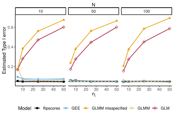
Figure 1: Estimated type I error considering $N\in\{10,50,100\}$ number of subjects and $n_{j}\in\{5,10,25,50\}$ repeated measurements. Each line represents one model and the grey area around the dashed black line represents the $0.95$ confidence bound for $\alpha=0.05$.

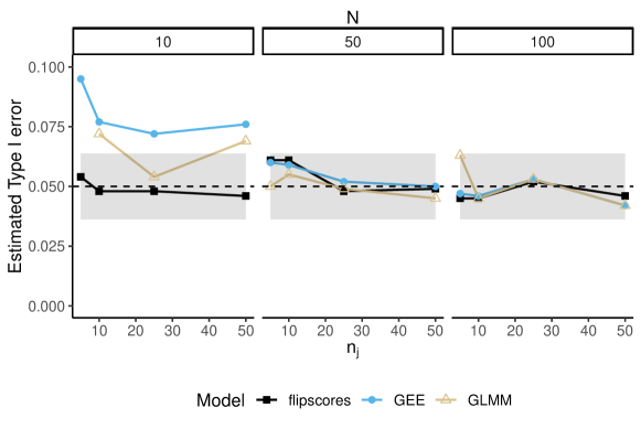
Figure 2: Zoom of Figure 1 considering the estimated type I error $\in[0,0.1]$. Estimated type I error considering $N\in\{10,50,100\}$ number of subjects and $n_{j}\in\{5,10,25,50\}$ repeated measurements. Each line represents one model and the grey area around the dashed black line represents the $0.95$ confidence bound for $\alpha=0.05$.

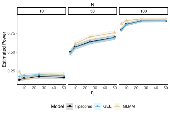
Figure 3: Estimated power considering $N\in\{10,50,100\}$ number of subjects and $n_{j}\in\{5,10,25,50\}$ repeated measurements. Each line represents one model with corresponding colored confidence bounds at $0.95$ level.

We can conclude from these simulations that the proposed method controlled the type I error for both small and large samples and for both few and many repeated measurements, unlike the two competitive methods considered, namely GEE and GLMM. In addition, a downside of the GLMM is that it requires the user to correctly specify the mixed model, which is often a problematic task, as mentioned above (Barr et al.,, 2013; Bates et al., 2015a, ).

6 Application

Adoption is a legal process in which an individual or a couple assumes permanent parental responsibility for a child who is not biologically related to them. The complexity of the adoption journey varies depending on factors such as the child’s age, the circumstances surrounding the adoption, and the child’s prior experiences. The dataset analyzed comes from a study of Santona et al., (2022), which is based on responses given by adoptive parents to reports called follow-ups. Follow-ups are periodic reports that provide information on the progress of the adoption, the child’s adjustment to the new environment, and their psychological and physical well-being. The Authorized Entity (i.e., an Italian institution that manages the adoption procedures), following the return of the adoptive family to Italy with the child, must carry out mandatory follow-ups required of adoptive families by the country of origin, which must then be transmitted to the foreign authority.

The sample analyzed consists of $534$ minors adopted between $2008$ and $2017$ through the Italian Childhood Aid Center (CIAI). The minors range in age from $0.8$ months to $12$ years upon arrival in Italy and come from different countries such as India, China, Burkina Faso, Colombia, Ethiopia, Thailand, Vietnam, and Cambodia. To study the trend over time of children’s physical development and health status detected at each follow-up, a new variable called Unhealth was created based on the following answers:

1. Physical development (regular versus irregular)

2. Psychomotor development (regular versus irregular)

3. Sleep-wake rhythm (regular versus irregular)

4. Nutrition (regular versus irregular)

5. Diseases (pathologies and/or developmental alterations versus none)

which belong to the life and medical areas of the follow-up report. The new variable, Unhealth is defined as a binary variable where $1$ means that at least one of the above health problems is present and $0$ means none are present.

In addition to the questions described above, we have various socio-demographic information for each child described in Table 1.

Variable name	Description
Sex	Sex of the child (Male/Female)
Time	Discrete variable indicating the survey time
Age	Age of the child when they arrived in the family
Country	Country of provenience of the child
Subject	Discrete variable indicating the child

Table 1: Description of the socio-demographic variables.

The health status is recorded multiple times for each child; the aim is to understand the development of this variable across time, taking into account the evident within-child variability. Covariates such as Age (median $5$ year, range: between $1$ month and $12$ years), Country ($8$ countries, proportions ranging from $1.2\%$ to $47.2\%$ ), and Sex (female 42.0%) defined in Table 1 are considered in the model as moderator variables. Figure 4 shows the relation between country and time. As it is visible from the plot, the number of follow-ups and the time – from the adoption – varies among countries, This is due to differing regulations.

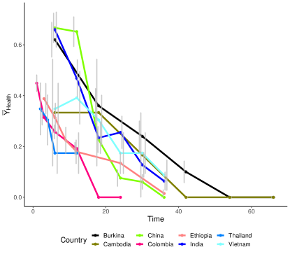
Figure 4: Sample proportion of children with an unhealthy status across time for each country. The grey bars indicate a $\approx 0.3$ confidence interval for each time point/country combination.

Here, we apply our proposed method presented in Section 3 and other two competitive approaches common in the literature, i.e., GEE and GLMM. The packages flipscores (Finos et al.,, 2023), geepack (Højsgaard et al.,, 2006), and lme4 (Bates et al., 2015b, ) are used respectively.

First of all, we want to underline that the functions of the package flipscores follow the structure of the most common models implemented in R, e.g., linear model (lm function), GLM (glm function), and GLMM (glmer function). In short, the main function flipscores, which estimates the proposed method, returns an object with a class similar to the glm, glmer object classes. All the functions the users generally used (e.g., to make plots, a summary of the results) can also be used with the flipscores’s output. The R command used for performing the analysis is described in Code 1.

Listing 1: R command used to compute robust statistical tests for binary longitudinal data by flipscores function.

⬇

mod <- flipscores(formula = Unhealth~Sex+Age+Country+Time,

data= db,

family = binomial,

id = db$Subject)

summary(mod)

anova(mod)

where db denotes the data.frame class object containing our data. The random effects are directly managed by specifying the variable that identifies the cluster (e.g., subject) in the id argument of the flipscores function. Therefore, as mentioned in Section 3, the problem of defining the correlation structure related to the GEE and GLMM models is solved in a simple way.

We start our analysis by estimating the GLMM with two random effects: a random slope defined by the survey time and random intercept defined by the subject variable. The fixed effects part is specified in the same way as defined in the right part of the formula object in Code 1. Using the default optimizer, i.e., a two-stage optimization, where the Bound Optimization BY Quadratic Approximation (BOBYQA) iterative algorithm (Powell et al.,, 2009) is used in the first stage and the Nelder-Mead approach (Lagarias et al.,, 1998) in the second one, the estimation process does not converge. This was solved by specifying the BOBYQA optimizer for both stages, increasing the maximum number of function evaluations to $200000$, leading to a high computational time (i.e., $\approx 4$ minutes). In contrast, GEE and flipscores reach a computational time equal to $35$ and $0.3$ seconds, respectively.

Table 2 shows the results of the flipscores analysis. The ANOVA detects significant effects for all variables included in the model. More specifically, the time from the arrival in the new family and the age of arrival decrease the probability of health issues, while males are more prone to them. The country of origin seems to be important as well. In particular, Burkina Faso – taken as the reference level – is the country with the highest coefficients, while all others have negative fitted values, with only Cambodia and India not being significantly different from Burkina Faso. Results of the GLMM and GEE methods are reported in Tables 3 and 4, respectively. In the GLMM case, we consider both intercept and random slopes; the results assuming only a random intercept are placed in Appendix B. The results are broadly similar, with all variables being significant in the ANOVA analysis and fitted coefficients having the same magnitude and sign. As for flipscores, in GEE Cambodia and India are the only nonsignificant coefficients. This is also true for the GLMM with the intercept as random effect only (see Appendix B), while by modeling both intercept and slopes as random, the nonsignificant ones are China and India (see Table 3). This again emphasizes the problem that the choice of the random part’s structure affects the results. This problem is bypassed by adopting the proposed flipscores approach.

Figures 6 and 6 give an intuition of the effects of the covariates estimated by flipscores on the probability of having at least one physical health problem.

Table 2: flipscores model results: summary of the model and related analysis of variance table.

Estimate Score Std. Error $z$ value Part. Cor $\Pr(>|z|)$ Intercept $2.2428$ $38.245$ $3.896$ $9.817$ $0.1713$ $0.0002$ Time $-0.1273$ $-5576.002$ $254.721$ $-21.891$ $-0.3924$ $0.0002$ Sex Male $0.3632$ $35.427$ $9.939$ $3.564$ $0.0650$ $0.0110$ Country Cambodia $-1.3042$ $-3.737$ $1.759$ $-2.125$ $-0.0382$ $0.1710$ Country China $-0.6331$ $-11.889$ $4.299$ $-2.765$ $-0.0492$ $0.0358$ Country Colombia $-2.1306$ $-43.117$ $3.952$ $-10.911$ $-0.1780$ $0.0002$ Country Ethiopia $-1.8146$ $-31.637$ $4.038$ $-7.835$ $-0.1370$ $0.0002$ Country India $-0.3095$ $-5.341$ $4.147$ $-1.288$ $-0.0231$ $0.3692$ Country Thailand $-2.2514$ $-24.232$ $3.328$ $-7.281$ $-0.1295$ $0.0002$ Country Vietnam $-0.9683$ $-11.520$ $3.483$ $-3.308$ $-0.0594$ $0.0344$ Age $-0.1229$ $-388.565$ $57.148$ $-6.799$ $-0.1245$ $0.0002$ Df Score $\Pr(>\text{Score})$ Time $1$ $0.2106$ $0.0002$ Sex $1$ $0.0357$ $0.0130$ Country $7$ $44.1424$ $0.0002$ Age $1$ $0.0687$ $0.0002$

Table 3: GLMM model results: summary of the model and related analysis of variance table.

	Estimate	Std. Error	$z$ value	$\Pr(>|z|)$
Intercept	$3.2157$	$0.4260$	$7.556$	$<0.001$
Time	$-0.2124$	$0.0150$	$-14.085$	$<0.001$
Sex Male	$0.6401$	$0.2002$	$3.197$	$0.0014$
Country Cambodia	$-1.9436$	$1.0781$	$-1.803$	$0.0714$
Country China	$-0.4745$	$0.4511$	$-1.052$	$0.2929$
Country Colombia	$-2.8972$	$0.3911$	$-7.408$	$<0.001$
Country Ethiopia	$-2.5099$	$0.4407$	$-5.695$	$<0.001$
Country India	$-0.2997$	$0.4705$	$-0.637$	$0.5241$
Country Thailand	$-3.1399$	$0.5844$	$-5.373$	$<0.001$
Country Vietnam	$-1.5479$	$0.5792$	$-2.672$	$0.0075$
Age	$-0.1843$	$0.0356$	$-5.178$	$<0.001$

	n. par	Sum Sq.	Mean Sq.	$F$ value
Time	$1$	$291.6240$	$291.6240$	$291.6240$
Sex	$1$	$10.3020$	$10.3020$	$10.3020$
Country	$7$	$149.4039$	$21.3434$	$21.3434$
Age	$1$	$28.7720$	$28.7720$	$28.7720$

Table 4: GEE results: summary of the model and related analysis of variance table.

	Estimate	Std.err	Wald test	$\Pr(>|W|)$
Intercept	$2.2428$	$0.2620$	$73.306$	$<0.001$
Time	$-0.1273$	$0.0067$	$362.167$	$<0.001$
Sex Male	$0.3632$	$0.1025$	$12.548$	$0.0004$
Country Cambodia	$-1.3042$	$0.7533$	$2.997$	$0.0834$
Country China	$-0.6331$	$0.2487$	$6.481$	$0.0109$
Country Colombia	$-2.1306$	$0.2344$	$82.654$	$<0.001$
Country Ethiopia	$-1.8146$	$0.2672$	$46.111$	$<0.001$
Country India	$-0.3095$	$0.2676$	$1.337$	$0.2475$
Country Thailand	$-2.2514$	$0.3362$	$44.831$	$<0.001$
Country Vietnam	$-0.9683$	$0.3409$	$8.067$	$0.0045$
Age	$-0.1229$	$0.0181$	$45.869$	$<0.001$

	Df	$\chi^{2}$ value	$\Pr(>|\chi^{2}|)$
Time	$1$	$239.8565$	$<0.001$
Sex	$1$	$13.1742$	$0.0004$
Country	$7$	$227.5656$	$<0.001$
Age	$1$	$45.8694$	$<0.001$

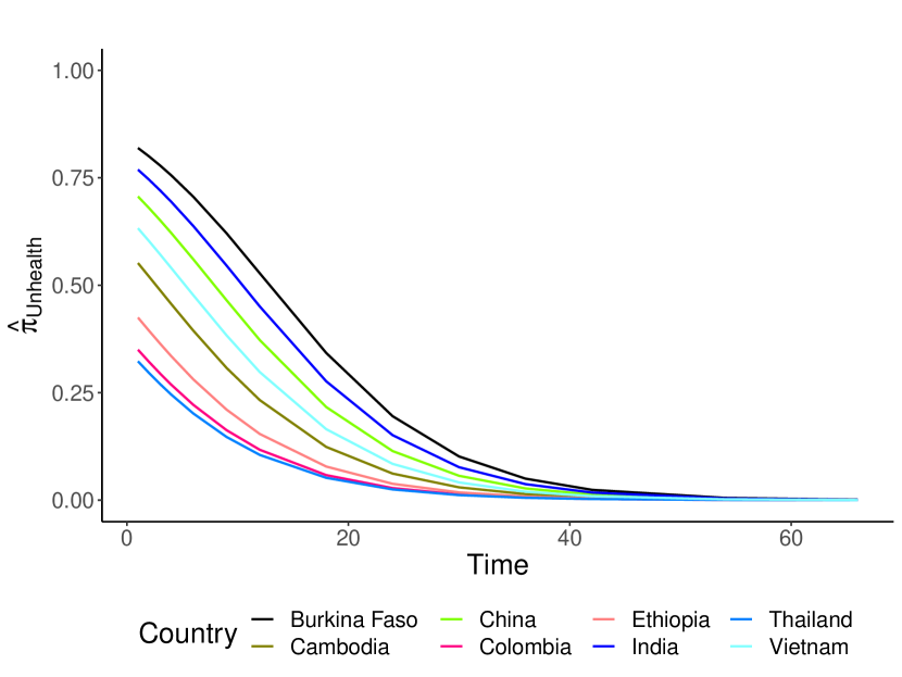
Figure 5: Estimated probabilities of being unhealthy for each country across time estimated by flipscores.

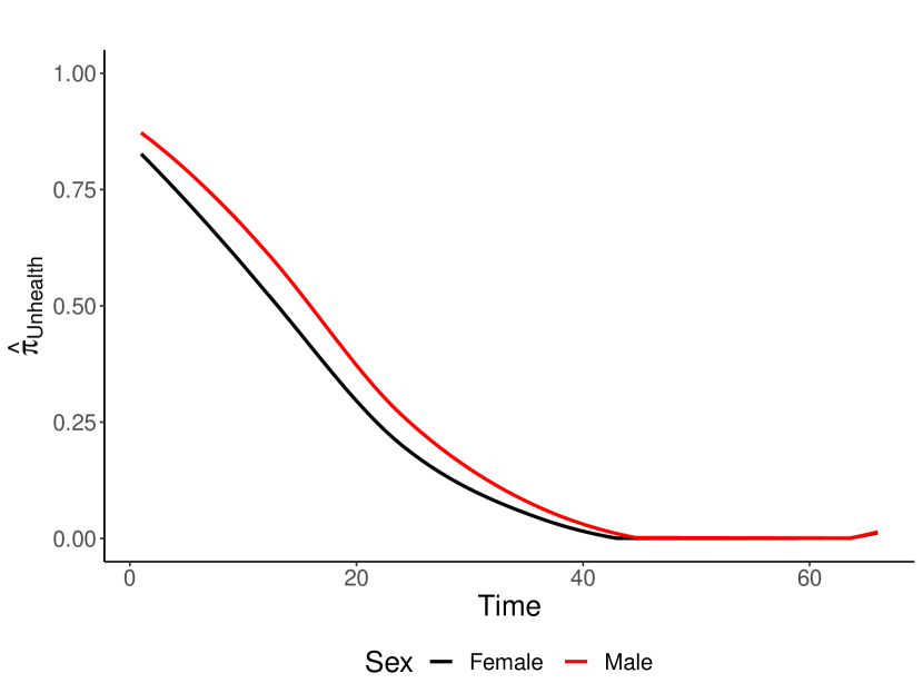
Figure 6: Estimated probabilities of being unhealthy divided by sex across age estimated by flipscores.

7 Discussion

The extension of the flipscores (Hemerik et al.,, 2020; De Santis et al.,, 2022) method proposed here accounts for heteroscedasticity between subjects and within-subject dependence, which are crucial considerations in statistical modeling. With existing methods, the heteroscedastic nature of data can introduce bias and compromise the validity of statistical inferences. Accounting for within-subject dependence is likewise essential for valid statistical inference. The proposed method is shown to have the required properties through mathematical proof, simulations, and real-world applications. These demonstrate our method’s superiority in terms of statistical power and control over false positive rates compared to conventional parametric methods. In addition, the proposed approach is able to handle several random effects without an explicit specification in the model. The researcher is not required to choose the random structure of the model (i.e., random intercept and random slope), as happens when the GLMM is used. The only prerequisite is a grasp of the underlying structure of data clusters in order to ensure the fulfillment of the exchangeability assumption under the null hypothesis. In contrast, specifying the random part of a GLMM is a complex process: no general solution is available for the problem of choosing between e.g., a parsimonious (Bates et al., 2015a, ) and a maximal (Barr et al.,, 2013) model. This choice, however, directly impacts the inferential conclusions.

Some limitations of the approach are to be discussed. In this work, we considered confounding variables at the cluster level (e.g., gender, nationality). The case of having confounding variables that vary within the subject will be explored in a later work. In fact, we noted that when confounding variables vary within subjects and are correlated with the variable of interest, the proposed method does not control type I error. This has also been found using quasi-likelihood-based methods such as GEE. The Appendix A shows results confirming these claims. However, the proposed method remains valid in several situations: (1) when the relationship between the dependent variable and covariates is linear under any scenario, (2) when the nuisance variable varying within-subject is uncorrelated with the variable of interest, (3) when the random effect occurs only as a random intercept under any structure of the nuisance variable. Another limitation includes handling more complex correlation structures such as crossed-random effects, since the whole-block exchangeability is then not satisfied. The cases described above and, in addition, the extension to the multivariate case (i.e., when we have more than one dependent variable) will be properly investigated in further works.

In conclusion, our research extends the applicability of permutation-based approaches in generalized linear mixed models, offering a flexible and reliable tool to overcome the limitations of traditional statistical parametric methods. With its ability to handle complex random effect structures and account for heteroscedasticity and within-subject dependence, our approach promises to advance statistical inference in psychometric research and beyond. As such, it opens up new avenues for exploring intricate relationships and dependencies within diverse datasets, expanding the horizons of statistical analysis in various fields.

Author contribution

AA: conceptualization, methodology, data curation, formal analysis, investigation, writing - original draft, writing - review & editing. JG: conceptualization, methodology, investigation, writing - review & editing, supervision. JH: conceptualization, methodology, investigation, writing - review & editing. LF: conceptualization, methodology, data curation, investigation, writing - review & editing, supervision.

Appendix A Simulation results

Figure A.1 represents the same situation as Figure 1 simulating without the random effect with respect to the covariate of interest $X_{ij}$, i.e., $D_{j}=0$. The corrected specified GLMM returns $5\%$ of the times a singularity warning and $0.5\%$ of the times a non-convergence issue, while the misspecified model encounters $74\%$ of the times a singularity warning. In these cases, we consider a $p$-value equals $1$. Finally, Figure A.2 shows the estimated power as Figure 3 again fixing $D_{j}=0$.

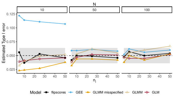
Figure A.1: Estimated type I error considering $N\in\{10,50,100\}$ number of subjects and $n_{j}\in\{5,10,25,50\}$ repeated measurements. Each line represents one model and the grey area around the dashed black line represents the $0.95$ confidence bounds for $\alpha=0.05$.

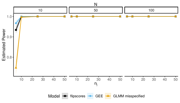
Figure A.2: Estimated power considering $N\in\{10,50,100\}$ number of subjects and $n_{j}\in\{5,10,25,50\}$ repeated measurements. Each line represents one model with corresponding colored confidence bounds at level $0.95$.

Finally, the scenario when the nuisance covariate $Z$ varies within the subject is represented. Figure A.3 shows the case when $Z$ is uncorrelated with $X$, while Figure A.3 illustrates the case when $Z$ and $X$ are correlated, imposing a correlation equals $0.5$. Focusing on Figure A.3, we can note that the correct specified GLMM does not fail in controlling the error only when both numbers of subjects and repeated measurements for each subject are large (i.e., $n_{j}\in\{25,50\}$ and $N\in\{50,100\}$). In addition, the asymptotic proprieties of GEE decay in the presence of a small number of subjects. Instead, the flipscores approach proposed maintains type I error control in all scenarios. Across all the simulations, the correctly specified GLMM encounters a convergence problem $3.31\%$ times, singularity issue $1.62\%$ times, and gives error $0.008\%$ of the times. In this case, we consider a p-values equal to $1$.

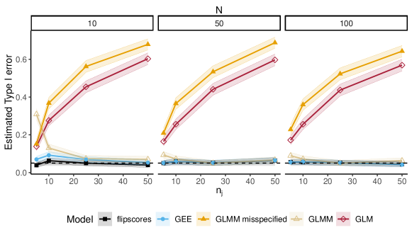
Figure A.3: Estimated type I error considering $N\in\{10,50,100\}$ number of subjects and $n_{j}\in\{5,10,25,50\}$ repeated measurements. Each line represents one model with corresponding colored confidence bounds at level $0.95$.

However, in the case of correlation between $X$ and $Z$, both GEE and flipscores approaches do not properly compute valid statistical tests. As discussed in the conclusion, we will explore this in a future paper. The intuition behind erroneous error control is that the score-based test statistic retains the random effect on the variable of interest correlated with the nuisance one in the case of nonlinearity between covariates and the dependent variable under the null hypothesis. In fact, the problem does not persist in the case of the dependent variable being normally distributed or if we simulate data with only a random intercept with a logistic link function.

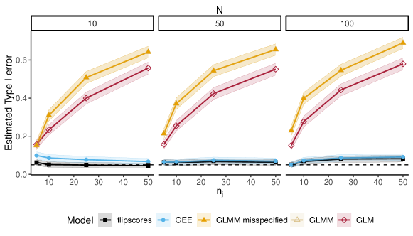
Figure A.4: Estimated type I error considering $N\in\{10,50,100\}$ number of subjects and $n_{j}\in\{5,10,25,50\}$ repeated measurements. Each line represents one model with corresponding colored confidence bounds at level $0.95$.

Appendix B Application

Table B.1: GLMM results assuming only the random intercept: summary of the model and related analysis of variance table.

	Estimate	Std. Error	$z$ value	$\Pr(>|z|)$
Intercept	$2.9887$	$0.3922$	$7.6194$	$<0.001$
Time	$-0.1697$	$0.0091$	$-18.7307$	$<0.001$
Sex Male	$0.5634$	$0.1909$	$2.9513$	$0.0032$
Country Cambodia	$-1.8076$	$1.0064$	$-1.7961$	$0.0725$
Country China	$-0.8781$	$0.3954$	$-2.2210$	$0.0264$
Country Colombia	$-2.9164$	$0.3557$	$-8.1989$	$<0.001$
Country Ethiopia	$-2.5128$	$0.4119$	$-6.1007$	$<0.001$
Country India	$-0.4908$	$0.4225$	$-1.1618$	$0.2453$
Country Thailand	$-3.1311$	$0.5585$	$-5.6058$	$<0.001$
Country Vietnam	$-1.3727$	$0.5266$	$-2.6068$	$0.0091$
Age	$-0.1682$	$0.0339$	$-4.9663$	$<0.001$

	n. par	Sum Sq.	Mean Sq.	$F$ value
Time	$1$	$279.6168$	$279.6168$	$279.6168$
Sex	$1$	$7.9399$	$7.9399$	$7.9399$
Country	$7$	$144.3750$	$20.6250$	$20.6250$
Age	$1$	$26.0067$	$26.0067$	$26.0067$

References

- Agresti, (2015) Agresti, A. (2015). Foundations of linear and generalized linear models. John Wiley & Sons.
- Azzalini, (2017) Azzalini, A. (2017). Statistical inference based on the likelihood. Routledge.
- Barr et al., (2013) Barr, D. J., Levy, R., Scheepers, C., and Tily, H. J. (2013). Random effects structure for confirmatory hypothesis testing: Keep it maximal. Journal of memory and language, 68(3):255–278.
- Barry et al., (2022) Barry, A., Oualkacha, K., and Charpentier, A. (2022). A new gee method to account for heteroscedasticity using asymmetric least-square regressions. Journal of Applied Statistics, 49(14):3564–3590.
- Basso and Finos, (2012) Basso, D. and Finos, L. (2012). Exact multivariate permutation tests for fixed effects in mixed-models. Communications in Statistics-Theory and Methods, 41(16-17):2991–3001.
- (6) Bates, D., Kliegl, R., Vasishth, S., and Baayen, H. (2015a). Parsimonious mixed models. arXiv preprint arXiv:1506.04967.
- (7) Bates, D., Mächler, M., Bolker, B., and Walker, S. (2015b). Fitting linear mixed-effects models using lme4. Journal of Statistical Software, 67:1–48.
- Carlin et al., (1999) Carlin, J. B., Wolfe, R., Coffey, C., and Patton, G. C. (1999). Analysis of binary outcomes in longitudinal studies using weighted estimating equations and discrete-time survival methods: prevalence and incidence of smoking in an adolescent cohort. Statistics in medicine, 18(19):2655–2679.
- Cnaan et al., (1997) Cnaan, A., Laird, N. M., and Slasor, P. (1997). Using the general linear mixed model to analyse unbalanced repeated measures and longitudinal data. Statistics in medicine, 16(20):2349–2380.
- Crowder, (1995) Crowder, M. (1995). On the use of a working correlation matrix in using generalised linear models for repeated measures. Biometrika, 82(2):407–410.
- De Santis et al., (2022) De Santis, R., Goeman, J. J., Hemerik, J., and Finos, L. (2022). Inference in generalized linear models with robustness to misspecified variances. arXiv preprint arXiv:2209.13918.
- Diggle et al., (1994) Diggle, P., Liang, K.-Y., and Zeger, S. L. (1994). Longitudinal data analysis. New York: Oxford University Press, 5:13.
- Finos and Basso, (2014) Finos, L. and Basso, D. (2014). Permutation tests for between-unit fixed effects in multivariate generalized linear mixed models. Statistics and Computing, 24:941–952.
- Finos et al., (2023) Finos, L., Goeman, J., Hemerik, J., and with contribution of Riccardo De Santis. (2023). flipscores: Robust Score Testing in GLMs, by Sign-Flip Contributions. R package version 1.3.0.
- Heagerty and Kurland, (2001) Heagerty, P. J. and Kurland, B. F. (2001). Misspecified maximum likelihood estimates and generalised linear mixed models. Biometrika, 88(4):973–985.
- Hemerik et al., (2020) Hemerik, J., Goeman, J. J., and Finos, L. (2020). Robust testing in generalized linear models by sign flipping score contributions. Journal of the Royal Statistical Society Series B: Statistical Methodology, 82(3):841–864.
- Højsgaard et al., (2006) Højsgaard, S., Halekoh, U., and Yan, J. (2006). The r package geepack for generalized estimating equations. Journal of statistical software, 15:1–11.
- Huang and Pan, (2021) Huang, Y. and Pan, J. (2021). Joint generalized estimating equations for longitudinal binary data. Computational Statistics & Data Analysis, 155:107110.
- Kherad-Pajouh and Renaud, (2010) Kherad-Pajouh, S. and Renaud, O. (2010). An exact permutation method for testing any effect in balanced and unbalanced fixed effect anova. Computational Statistics & Data Analysis, 54(7):1881–1893.
- Lagarias et al., (1998) Lagarias, J. C., Reeds, J. A., Wright, M. H., and Wright, P. E. (1998). Convergence properties of the nelder–mead simplex method in low dimensions. SIAM Journal on optimization, 9(1):112–147.
- Laird and Ware, (1982) Laird, N. M. and Ware, J. H. (1982). Random-effects models for longitudinal data. Biometrics, pages 963–974.
- Lee and Braun, (2012) Lee, O. E. and Braun, T. M. (2012). Permutation tests for random effects in linear mixed models. Biometrics, 68(2):486–493.
- Lehmann and Romano, (2022) Lehmann, E. L. and Romano, J. P. (2022). Multivariate permutation tests: with applications in biostatistics. Springer.
- Liang and Zeger, (1986) Liang, K.-Y. and Zeger, S. L. (1986). Longitudinal data analysis using generalized linear models. Biometrika, 73(1):13–22.
- Maas and Hox, (2004) Maas, C. J. and Hox, J. J. (2004). Robustness issues in multilevel regression analysis. Statistica Neerlandica, 58(2):127–137.
- Pesarin, (2001) Pesarin, F. (2001). Multivariate permutation tests: with applications in biostatistics.
- Powell et al., (2009) Powell, M. J. et al. (2009). The bobyqa algorithm for bound constrained optimization without derivatives. Cambridge NA Report NA2009/06, University of Cambridge, Cambridge, 26.
- Rao Chaganty and Joe, (2004) Rao Chaganty, N. and Joe, H. (2004). Efficiency of generalized estimating equations for binary responses. Journal of the Royal Statistical Society Series B: Statistical Methodology, 66(4):851–860.
- Santona et al., (2022) Santona, A., Tognasso, G., Miscioscia, C. L., Russo, D., and Gorla, L. (2022). Talking about the birth family since the beginning: The communicative openness in the new adoptive family. International Journal of Environmental Research and Public Health, 19(3):1203.
- Sullivan Pepe and Anderson, (1994) Sullivan Pepe, M. and Anderson, G. L. (1994). A cautionary note on inference for marginal regression models with longitudinal data and general correlated response data. Communications in statistics-simulation and computation, 23(4):939–951.
- Sutradhar and Das, (2000) Sutradhar, B. C. and Das, K. (2000). On the accuracy of efficiency of estimating equation approach. Biometrics, 56(2):622–625.
- Tuerlinckx et al., (2006) Tuerlinckx, F., Rijmen, F., Verbeke, G., and De Boeck, P. (2006). Statistical inference in generalized linear mixed models: A review. British Journal of Mathematical and Statistical Psychology, 59(2):225–255.
- Vonesh and Chinchilli, (1996) Vonesh, E. and Chinchilli, V. M. (1996). Linear and nonlinear models for the analysis of repeated measurements. CRC press.
- Wang and Carey, (2003) Wang, Y.-G. and Carey, V. (2003). Working correlation structure misspecification, estimation and covariate design: implications for generalised estimating equations performance. Biometrika, 90(1):29–41.
- Winkler et al., (2014) Winkler, A. M., Ridgway, G. R., Webster, M. A., Smith, S. M., and Nichols, T. E. (2014). Permutation inference for the general linear model. Neuroimage, 92:381–397.