Bagging cross-validated bandwidths with application to Big Data

Abstract

Hall & Robinson (2009) proposed and analyzed the use of bagged cross-validation to choose the bandwidth of a kernel density estimator. They established that bagging greatly reduces the noise inherent in ordinary cross-validation, and hence leads to a more efficient bandwidth selector. The asymptotic theory of Hall & Robinson (2009) assumes that $N$, the number of bagged subsamples, is $\infty$. We expand upon their theoretical results by allowing $N$ to be finite, as it is in practice. Our results indicate an important difference in the rate of convergence of the bagged cross-validation bandwidth for the cases $N=\infty$ and $N<\infty$. Simulations quantify the improvement in statistical efficiency and computational speed that can result from using bagged cross-validation as opposed to a binned implementation of ordinary cross-validation. The performance of the bagged bandwidth is also illustrated on a real, very large, data set. Finally, a byproduct of our study is the correction of errors appearing in the Hall & Robinson (2009) expression for the asymptotic mean squared error of the bagging selector.

Keywords: Bagging, Bandwidth, Big data, Cross-validation, Kernel density

Introduction

Cross-validation is a rough-and-ready method of model selection that predates an early exposition of the method by Stone (1974). In its simplest form, cross-validation consists of dividing one’s data set into two parts, using one part to build one or more models, and then predicting the data in the second part with the models so-built. In this way, one can objectively compare the predictive ability of different models. The leave-one-out version of cross-validation is somewhat more involved. It excludes one datum from the data set, fits a model from the remaining observations, uses this model to predict the datum left out, and then repeats this process for all the data.

While leave-one-out cross-validation is a very useful method, due in no small part to its wide applicability, it does have its drawbacks. In the context of smoothing parameter selection for function estimation, it has been regarded skeptically for many years owing to its large variability (see, e.g. Park & Marron, 1990). A number of modified versions of cross-validation have been proposed in an effort to produce more stable smoothing parameter selectors. These include partitioned cross-validation (Marron, 1987; Bhattacharya & Hart, 2016), proposals of Stute (1992) and Feluch & Koronacki (1992), smoothed cross-validation (Hall et al., 1992), one-sided cross-validation (Hart & Yi, 1998; Miranda et al., 2011), a bagged version of cross-validation (Hall & Robinson, 2009), indirect cross-validation (Savchuk et al., 2010) and DO-validation (Mammen et al., 2011).

The current paper revisits the application of bagging to the selection of a kernel density estimator’s bandwidth. Given a random sample of size $n$ from an unknown density $f$, bagging consists of selecting $N$ subsamples of size $m<n$, each without replacement, from the $n$ observations. One then computes a cross-validation bandwidth from each of the $N$ subsets, averages them, and then scales the average down appropriately to account for the fact that $m<n$. It is well-known that the use of bagging can lead to substantial reductions in the variability of an estimator that is nonlinear in the observations (see Friedman & Hall, 2007). Indeed, this is true in the bandwidth selection problem, as demonstrated in Hall & Robinson (2009).

A method closely related to bagging is partitioned cross-validation (Marron, 1987), wherein the data set is partitioned into mutually exclusive subsets, and a bandwidth is computed from each subset. One may then average these bandwidths and rescale as in bagging. A little thought reveals that the statistical properties of bagging and a replicated version of partitioned cross-validation are essentially equivalent, and hence to fix ideas we consider only bagging in this paper.

Two other popular methods of bandwidth selection are the plug-in method of Sheather & Jones (1991) and the bootstrap (Cao, 1993). It is worth mentioning that bagged versions of these two methodologies could also be considered. Some readers might argue that plug-in methods are more efficient than any version of cross-validation and hence should be the method of choice. However, Loader (1999) challenges this notion and provides good reasons for not discarding cross-validatory methods.

The main contributions of our paper are as follows:

(i) In the case $N=\infty$, we provide a correct expression for the asymptotic mean squared error of the bagged bandwidth. The analogous expression given by Hall & Robinson (2009) is in error. Their variance approximation is of too large an order, thus downplaying the actual reduction in variance that is possible with the use of bagging. In addition, we provide an expression for the first order bias of the bagged bandwidth and show that the Hall & Robinson (2009) bias approximation is actually of smaller order in terms of sample size. The same bias error appears in the article of Marron (1987). See Appendix 4.

(ii) We provide a first order approximation to the variance in the case where $N$ is finite, which, of course, is the case in practice. This is important because even if $N=n$, the asymptotic variance of the bagged bandwidth is of a different order than it is when $N=\infty$. The relevance of this result is immediate for massive data sets, since in such cases taking $N$ as large as $n$ can be prohibitive computationally.

(iii) We provide an automatic method to estimate the best subsample size, in the sense of minimum mean squared error.

(iv) Both the automatic method and the bagged bandwidth selector have been implemented into an R (R Development Core Team, 2020) package, called baggedcv (Barreiro-Ures et al., 2019), which is already available at CRAN.

Methodology

Let $X_{1},\ldots,X_{n}$ be a random sample from a density $f$, and consider estimating $f(x)$ by the kernel estimator (Parzen, 1962; Rosenblatt, 1956)

$$\hat{f}_{h}(x)=\frac{1}{nh}\sum_{i=1}^{n}K\left(\frac{x-X_{i}}{h}\right),$$

where $K$ is a symmetric kernel function and $h>0$ is the bandwidth or smoothing parameter. Making a good choice of the bandwidth is crucial to obtaining a good density estimate. An oft-used criterion for defining a good bandwidth is based on mean integrated squared error (MISE), defined by:

$$M(h)=E\left[\int_{-\infty}^{\infty}\left\{\hat{f}_{h}(x)-f(x)\right\}^{2}\,{\rm d}x\right].$$

Suppose that $f$ has two continuous derivatives. As shown by, for example, Silverman (1986), the minimizer, $h_{n0}$, of $M(h)$ with respect to $h$ is asymptotic to $h_{na}=Cn^{-1/5}$, as $n\rightarrow\infty$, where

$$C=\left\{\frac{R(K)}{\mu_{2}(K)^{2}R(f^{\prime\prime})}\right\}^{1/5},$$ (1)

$R(g)=\int g^{2}(x)\,{\rm d}x$ and $\mu_{j}(g)=\int x^{j}g(x)\,{\rm d}x$ ($j=0,1,\ldots$), provided that these integrals exist finite. Ideally, one would use $h_{n0}$ as a bandwidth in the estimator $\hat{f}_{h}$, but of course $h_{n0}$ depends on $f$ and so this is not feasible. A means of estimating $h_{n0}$ is based on cross-validation.

The leave-one-out cross-validation criterion can be written as:

$$CV(h)=\int_{-\infty}^{\infty}\hat{f}_{h}(x)^{2}\,{\rm d}x-\frac{2}{n}\sum_{i=1}^{n}\hat{f}_{h}^{i}(X_{i}),\quad h>0,$$

where $\hat{f}_{h}^{i}$ is a kernel estimate computed with the $n-1$ observations other than $X_{i}$. It is easily shown that, for any $h>0$, $CV(h)$ is an unbiased estimator of $M(h)-R(f)$. It seems natural then to estimate $h_{n0}$ by $\hat{h}_{n}$, the minimizer of $CV(h)$. Hall & Marron (1987) show that

$$n^{1/10}\left(\frac{\hat{h}_{n}-h_{n0}}{h_{n0}}\right)\to Z$$ (2)

in distribution, where $Z$ is normally distributed with mean 0. The good news here is that the relative error $(\hat{h}-h_{n0})/h_{n0}$ converges to 0 in probability, as $n\rightarrow\infty$. The bad news is that the rate of convergence is very slow, $n^{-1/10}$, which confirms the large variability of cross-validation alluded to in the introduction.

We now explain how bagging may be applied in the cross-validation context. A random sample $X_{1}^{*},\ldots,X_{m}^{*}$ is drawn without replacement from $X_{1},\ldots,X_{n}$, where $m<n$. This subsample is used to calculate a least squares cross-validation bandwidth $\hat{h}_{m}$. A rescaled version of $\hat{h}_{m}$, $\tilde{h}_{m}=(m/n)^{1/5}\hat{h}_{m}$, is a feasible estimator of the optimal MISE bandwidth, $h_{n0}$, for $\hat{f}_{h}$. Bagging consists of repeating the resampling independently $N$ times, leading to $N$ rescaled bandwidths $\tilde{h}_{m,1},\ldots,\tilde{h}_{m,N}$. The bagging bandwidth is then defined to be

$$\hat{h}(m,N)=\frac{1}{N}\sum_{i=1}^{N}\tilde{h}_{m,i}.$$ (3)

This approach was first proposed and studied by Hall & Robinson (2009).

It is worth mentioning that an alternative approach is to apply bagging to the cross-validation curves, wherein one averages the cross-validation curves from $N$ independent resamples of size $m$, finds the minimizer of the average curve, and then rescales the minimizer as before. The asymptotic properties of the two approaches are equivalent, but we prefer bagging the bandwidths since doing so requires less communication between resamples.

Asymptotic results

In this section, we provide asymptotic expressions for the bias and variance of the bagging bandwidth (3). Hall & Robinson (2009) studied this selector only in the case $N=\infty$. We find that the expression they give for the variance of (3), at $N=\infty$, is in error. We provide a correct expression for this variance, and, more importantly, study the case of finite $N$, since there is an important interplay between the values of $m$ and $N$. Of course, in practice it is not possible to use $N=\infty$, and indeed there is a computational motivation for limiting the size of $N$. We will show that if $N$ is, for example, of order $n$, then the rate of convergence of the variance to 0 is different than in the case $N=\infty$. This is a new result that does not arise from the method of proof used in Hall & Robinson (2009).

Obviously $E\{\hat{h}(m,N)\}=E\{(m/n)^{1/5}\hat{h}_{m}\}$, and hence it suffices to know the bias of $(m/n)^{1/5}\hat{h}_{m}$ as an estimator of $h_{n0}$. We have

$$E\left\{(m/n)^{1/5}\hat{h}_{m}\right\}-h_{n0}=B_{\rm rescale}(m,n)+(m/n)^{1/5}B_{\rm CV}(m),$$

where

$$B_{\rm rescale}(m,n)=(m/n)^{1/5}h_{m0}-h_{n0}\quad{\rm and}\quad B_{\rm CV}(m)=E(\hat{h}_{m})-h_{m0}.$$

The rescaling bias, $B_{\rm rescale}(m,n)$, is well-understood. Marron (1987) shows that

$$B_{\rm rescale}(m,n)=\mu_{\rm rescale}m^{-2/5}n^{-1/5}+o\left(m^{-2/5}n^{-1/5}\right),$$

where

$$\mu_{\rm rescale}=\frac{R(K)^{3/5}R(f^{\prime\prime\prime})\mu_{4}(K)}{20R(f^{\prime\prime})^{8/5}}.$$

Hall & Robinson (2009) also provide an expression for $B_{\rm rescale}(m,n)$, although their rate is in error.

The other bias component, $B_{\rm CV}$, is the bias inherent to cross-validation itself, and has a curious history in the literature. In establishing (2), Hall & Marron (1987) write

$$\hat{h}_{n}-h_{n0}=\xi_{n}+e_{n},$$ (4)

where $E(\xi_{n})=0$ and $e_{n}=o_{p}(\xi_{n})$, and hence $B_{\rm CV}(n)$ is lost in the term $e_{n}$. Doing so is acceptable in the case of ordinary cross-validation because of the fact that ${\rm var}(\xi_{n})$ is so large. In the case of bagging, however, when ${\rm var}\{\hat{h}(m,N)\}$ becomes sufficiently small, one should no longer ignore $B_{\rm CV}(m)$, although this seems to be what both Marron (1987) and Hall & Robinson (2009) did.

In Appendix 1 as part of the proof of the main theorem stated below, we prove that $n^{2/5}e_{n}$ converges in distribution to a random variable with mean

$$\mu_{\rm CV}=-\frac{8R(f)\int V(u)W(u)du}{25R(K)^{8/5}R(f^{\prime\prime})^{2/5}},$$ (5)

where $V$ and $W$ are functions determined completely by $K$. For example, $\int V(u)W(u)du=0.1431285$ in the case of the standard normal kernel.

The following assumptions are made in order to prove Theorem 1:

Assumption 1.

As $m,n\to\infty$, $m=o(n)$ and $N$ tends to a positive constant or $\infty$.

Assumption 2.

$K$ is a symmetric and twice differentiable density function having, without loss of generality, variance $\mu_{2}(K)=1$.

Assumption 3.

As $u\to\infty$, both $K(u)$ and $K^{\prime}(u)$ are $o\{\exp(-a_{1}u^{a_{2}})\}$ for positive constants $a_{1}$ and $a_{2}$.

Assumption 4.

The first three derivatives of $f$ exist and are bounded and continuous.

Theorem 1.

Under Assumptions 1–4, the bias of the bagged bandwidth (3) is:

$$E\left\{\hat{h}(m,N)\right\}-h_{n0}=m^{-1/5}n^{-1/5}\left(\mu_{\rm CV}+\mu_{\rm rescale}m^{-1/5}\right)+o\left(m^{-1/5}n^{-1/5}\right)$$ (6)

and its variance is:

$${\rm var}\left\{\hat{h}(m,N)\right\} = AC^{2}m^{-1/5}n^{-2/5}\left\{\frac{1}{N}+\left(\frac{m}{n}\right)^{2}\right\}$$

$$+ o\left(\frac{m^{-1/5}n^{-2/5}}{N}+m^{9/5}n^{-12/5}\right),$$

where $A$ and $C$ are constants defined by (22) in Appendix 1 and (1), respectively.

Expression (3) implies that at $N=\infty$ the asymptotic variance of the bagged bandwidth is completely determined by the covariance between bandwidths for two different resamples. Furthermore, to first order, as derived in Bhattacharya & Hart (2016), the correlation between bagged bandwidths from different resamples is independent of $f$ and equal to $(m/n)^{2}$. This correlation is smaller when $m$ is smaller, which is due to the fact that two resamples will usually have fewer data values in common when $m$ is smaller. In fact, taking $N=\infty$ yields the approximation

$${\rm var}\left\{\hat{h}(m,N)\right\}=AC^{2}m^{9/5}n^{-12/5}+o\left(m^{9/5}n^{-12/5}\right),$$ (8)

which matches precisely one of the two summands in expression (13) of Hall & Robinson (2009). It can be shown that the other summand, rather than being the dominant term, as claimed by Hall & Robinson (2009), is actually negligible in comparison to (8).

It is easily verified that the choice of $m$ that minimizes the main term of (1) is asymptotic to $n/(3\sqrt{N})$. Therefore, if $N=n$, say, then the fastest rate at which ${\rm var}\{\hat{h}(m,N)\}/h_{n0}^{2}$ can converge to 0 is $n^{-11/10}$. In contrast, when $N=\infty$, the rate of convergence of ${\rm var}\{\hat{h}(m,N)\}/h_{n0}^{2}$ can be arbitrarily close to $n^{-2}$ by allowing $m$ to increase sufficiently slowly with $n$. This makes it clear that the properties of the bagged bandwidth are substantially affected by how many subsamples are taken, and hence it does not suffice to analyze the bagged bandwidth by setting $N=\infty$.

It is remarkable how much stability bagging can provide. Whether $N$ is $\infty$ or merely tending to $\infty$, ${\rm var}\{\hat{h}(m,N)/h_{n0}\}$ can converge to 0 faster than the usual parametric rate of $n^{-1}$. This is in stark contrast to the extremely slow rate of $n^{-1/5}$ for ordinary cross-validation. Unfortunately, this extreme stability cannot be fully taken advantage of since the bagged bandwidth is more biased than the ordinary cross-validation bandwidth. The largest reductions in variance are associated with small values of $m$, but it turns out that small $m$ yields the largest bias.

As seen in (6), the bias term $B_{\rm CV}$, that has been ignored to date, is of a larger order than the rescaling bias. This and the fact that $\mu_{\rm CV}<0$ suggest that the bagged bandwidth would tend to be smaller than the optimal bandwidth $h_{n0}$. However, our experience in numerous simulations is that the bagged bandwidth actually tends to be larger than $h_{n0}$. The explanation for this phenomenon is simple: $\mu_{\rm rescale}>0$ and $\mu_{\rm rescale}$ is larger than $|\mu_{CV}|$ in every case we have checked. Indeed, we have not found a case where $\mu_{\rm rescale}/|\mu_{CV}|$ is less than 2, and it appears that there is no limit to how large this ratio can be.

Table 1 provides the constants $\mu_{\rm rescale}$ and $\mu_{CV}$ for several densities. Two patterns are apparent here: (i) the heavier the tail of the density, the more dominant is the rescaling bias, and (ii) the rescaling bias is more dominant for multimodal mixtures of normals than for the normal itself. Define $m_{\rm crit}$ to be the smallest subsample size at which the asymptotic mean of the bagged bandwidth is not larger than the optimal MISE bandwidth, $h_{n0}$. Since the ratio $\mu_{\rm rescale}/\mu_{CV}$ is invariant to location and scale, it follows that the values of $m_{\rm crit}$ for any normal, logistic or Cauchy distribution are the same as in Table 1. Except in the case of the Beta$(5,5)$ and normal densities, the values of $m_{\rm crit}$ are very large, especially considering that a good choice for $m$ is usually much smaller than $n$, as we shall subsequently see. So, in spite of what the asymptotics suggest, it will often be the case that the bagged bandwidth is larger on average than the optimal bandwidth. This is a classic case of asymptotics not kicking in until the sample size is extremely large.

Table 1: Bias constants and critical $m$ ($m_{\rm crit}$) for the Gaussian kernel. The claw density (Marron & Wand, 1992) is a symmetric density mixture of six normals with five modes (see Section Appendix 2. Simulation study, for the definition of the claw density). The bimodal mixture of two normals has parameters $\mu=(-1.5,1.5)$, $\sigma=(0.5,0.5)$ and $w=(0.5,0.5)$, where $\mu$, $\sigma$ and $w$ are the mean, standard deviation and weight vectors, respectively, for the density mixture (see Section Appendix 2. Simulation study, for the notation used for a normal mixture density).

Density	$\mu_{\rm rescale}$	$\mu_{\rm CV}$	$m_{\rm crit}$
Beta$(5,5)$	$0.06554$	$-0.03070$	$45$
Standard normal	$0.44565$	$-0.18216$	$88$
Standard logistic	$0.92556$	$-0.25787$	$596$
Bimodal mixture of two normals	$0.32809$	$-0.05988$	$4936$
Standard Cauchy	$1.24349$	$-0.09793$	$330,154$
Claw	$0.22774$	$-0.00766$	$>10^{7}$

• The bimodal mixture of two normals has parameters $\mu=(-1.5,1.5)$, $\sigma=(0.5,0.5)$ and $w=(0.5,0.5)$, where $\mu$, $\sigma$ and $w$ are the mean, standard deviation and weight vectors, respectively, for the density mixture (see Section Appendix 2. Simulation study, for the notation used for a normal mixture density).

Choosing an optimal subsample size

In practice, for fixed $n$ and $N$, our results allow one to estimate an optimal subsample size, $m_{0}$. This quantity is defined to be the minimizer of the asymptotic mean squared error (AMSE) of $\hat{h}(m,N)$ with respect to $m$:

$$\textsc{AMSE}\left\{\hat{h}(m,N)\right\} = AC^{2}m^{-1/5}n^{-2/5}\left\{\frac{1}{N}+\left(\frac{m}{n}\right)^{2}\right\}$$ (9)

$$+ m^{-2/5}n^{-2/5}\left(\mu_{CV}+\mu_{rescale}m^{-1/5}\right)^{2}.$$

Since $\mu_{rescale}$, $\mu_{CV}$, $A$ and $C$ are unknown, we propose the following method to estimate

$$m_{0}=\operatorname*{arg\,min}\limits_{m>1}\textsc{AMSE}\left\{\hat{h}(m,N)\right\}.$$

1. Consider $s$ subsamples of size $r<n$, drawn without replacement from the original sample of size $n$.

2. For each of these subsamples, fit a normal mixture model. To fit a mixture model with a given number of components, use the expectation-maximization algorithm initialized by hierarchical model-based agglomerative clustering. Then, estimate the optimal number of mixture components by using BIC, the Bayesian information criterion. In practice, this process is performed employing the R package mclust (see Scrucca et al., 2016).

3. Use $R(\hat{f}_{i})$, $R(\hat{f}_{i}^{\prime\prime})$ and $R(\hat{f}_{i}^{\prime\prime\prime})$ to estimate $A$, $C$, $\mu_{CV}$ and $\mu_{rescale}$, where $\hat{f}_{i}$ denotes the density function of the normal mixture fitted to the $i$th subsample. Denote these estimates by $\hat{A}_{i}$, $\hat{C}_{i}$, $\hat{\mu}_{CV,i}$ and $\hat{\mu}_{rescale,i}$.

4. Compute the bagged estimates of the unknown constants, that is, $\hat{D}=\frac{1}{s}\sum\limits_{i=1}^{s}\hat{D}_{i}$, where $\hat{D}_{i}$ can be $\hat{A}_{i}$, $\hat{C}_{i}$, $\hat{\mu}_{CV,i}$ or $\hat{\mu}_{rescale,i}$, and obtain $\widehat{\textsc{AMSE}}\{\hat{h}(m,N)\}$ by plugging these bagged estimates into (9).

5. Finally, estimate $m_{0}$ by:

   $$\hat{m}_{0}=\operatorname*{arg\,min}\limits_{m>1}\widehat{\textsc{AMSE}}\left\{\hat{h}(m,N)\right\}.$$

Regarding the selection of $s$ and $r$ in Step 1, we have performed some empirical tests and observed that the estimation of $h_{n0}$ by $\hat{h}(\hat{m}_{0},N)$ is quite robust to the values of these parameters. For example, values of $s\simeq 50$ and $r\simeq 0.01n$ have provided, in general, good results.

Discussion

The finite sample behaviour of a bagged cross-validation bandwidth was investigated by means of a simulation study, and its practical performance was illustrated using a large data set involving flight delays. These experiments, included in Appendixes 2 and 3, show that subsampling can significantly reduce computing time relative to a binned version of leave-one-out cross-validation.

As mentioned in Section 1, bagged versions of other bandwidth selection methodologies, such as plug-in and bootstrap, could be considered. While both cross-validation and bootstrap approaches try to estimate $h_{n0}$, plug-in bandwidths are estimators of $h_{na}$, the bandwidth minimizing the asymptotic MISE, and hence they only need to estimate $R(f^{\prime\prime})$. It is worth noting that there is a clear similarity between the three methods. Both cross-validation (Scott & Terrell, 1987) and bootstrap (Cao, 1993) bandwidths are minimizers of criteria of the form:

$$\sum\limits_{(i,j)\in\cal{I}}H_{nhg}(X_{i}-X_{j})+\frac{R(K)}{nh},$$ (10)

where ${\cal I}\subset\{1,\ldots,n\}\times\{1,\ldots,n\}$ and $H_{nhg}$ is a function that may depend on the sample size, $n$, the bandwidth, $h$, and a pilot bandwidth, $g$. Note that $g$ plays a role only in the bootstrap criterion. Although plug-in bandwidths are not solutions to a minimization problem, the nonparametric estimation of $R(f^{\prime\prime})$ using pilot bandwidth $g$ requires working with a $U$-statistic like the one given in the first term in (10), which would only depend on $n$ and $g$. Due to the nonlinearity of (10) with respect to the observations, it stands to reason that a bagged implementation of these methods could reduce their variability, as in the case of cross-validation.

Appendix 1. Theoretical results

This Appendix includes the proof of Theorem 1, providing the asymptotic bias and variance of our bagged cross-validation bandwidth.

To prove Theorem 1, we establish one lemma in advance.

Lemma 1.

Under Assumptions 1–4,

$$n^{1/5}CV^{\prime\prime\prime}(\tilde{h}_{n})=o_{P}(1),$$ (11)

where $\tilde{h}_{n}$ is a bandwidth between the cross-validation bandwidth $\hat{h}_{n}$ and the MISE minimizer $h_{n0}$.

Proof.

First, we write

$$n^{1/5}CV^{\prime\prime\prime}(\tilde{h}_{n})=\alpha_{1}+\alpha_{2},$$ (12)

with $\alpha_{1}=n^{1/5}CV^{\prime\prime\prime}(h_{n0})$ and $\alpha_{2}=n^{1/5}\left\{CV^{\prime\prime\prime}(\tilde{h}_{n})-CV^{\prime\prime\prime}(h_{n0})\right\}$. To prove Lemma 1 it is sufficient to show that $\alpha_{1}=o_{P}(1)$ and $\alpha_{2}=o_{P}(1)$. In order to study the term $\alpha_{1}$, we first consider the asymptotic MISE of the Parzen–Rosenblatt estimator of the density function. It is well-known that if $K$ is a second order symmetric kernel function and considering that $K$ has variance $1$, as stated in Assumption 2, the MISE is:

$$M(h)=\frac{R(K)}{nh}+\frac{1}{4}h^{4}R(f^{\prime\prime})+o\left\{(nh)^{-1}+h^{4}\right\},$$

and, hence,

$$M^{\prime\prime\prime}(h)=-\frac{6R(K)}{nh^{4}}+6hR(f^{\prime\prime})+o\left\{(nh^{4})^{-1}+h\right\}.$$

Since

$$-\frac{6R(K)}{nh_{na}^{4}}+6h_{na}R(f^{\prime\prime})=0,$$

where $h_{na}$ denotes the bandwidth minimizing the asymptotic MISE, it follows immediately that $n^{1/5}M^{\prime\prime\prime}(h_{n0})$ converges to 0. Now, we can write

$$n^{1/5}CV^{\prime\prime\prime}(h_{n0})=n^{1/5}M^{\prime\prime\prime}(h_{n0})+n^{1/5}\eta_{n},$$

where $\eta_{n}=CV^{\prime\prime\prime}(h_{n0})-M^{\prime\prime\prime}(h_{n0})$. Thus, to prove that $\alpha_{1}=o_{P}(1)$, it is sufficient to prove that

$$\eta_{n}=o_{P}\left(n^{-1/5}\right),$$ (13)

or, by Markov’s inequality, that $n^{2/5}{\rm var}\{CV^{\prime\prime\prime}(h_{n0})\}=o(1)$. It is easy to prove that, for every $r\geq 1$,

$$CV^{(r)}(h)=M^{(r)}(h)+\frac{1}{n(n-1)}\sum_{i\neq j}\bar{\gamma}_{nh}^{(r)}(X_{i}-X_{j}),$$ (14)

where

$$\gamma_{n}(u)=\frac{n-1}{n}K*K(u)-2K(u),$$

$$\gamma_{nh}(u)=\gamma_{n}(u/h)/h,$$

$$\bar{\gamma}_{nh}(u)=\gamma_{nh}(u)-E\{\gamma_{nh}(X_{1}-X_{2})\}$$

and

$$\bar{\gamma}_{nh}^{(r)}(u)=\frac{{\rm d}^{r}\bar{\gamma}_{nh}(u)}{{\rm d}h^{r}}.$$

Therefore,

$${\rm var}\left\{CV^{\prime\prime\prime}(h)\right\}=\frac{1}{n^{2}(n-1)^{2}}\sum_{\begin{subarray}{c}i,j,k,l=1\\ i\neq j\\ k\neq l\end{subarray}}^{n}{\rm cov}\left\{\Psi_{3}(X_{i}-X_{j}),\Psi_{3}(X_{k}-X_{l})\right\},$$

where

$$\Psi_{3}(u)=\frac{{\rm d}^{3}\gamma_{nh}(u)}{{\rm d}h^{3}}=-\left\{\frac{6}{h^{4}}\gamma_{n}(u/h)+\frac{18u}{h^{5}}\gamma_{n}^{\prime}(u/h)+\frac{9u^{2}}{h^{6}}\gamma_{n}^{\prime\prime}(u/h)+\frac{u^{3}}{h^{7}}\gamma_{n}^{\prime\prime\prime}(u/h)\right\}.$$

Counting the different possible cases, we get

$${\rm var}\left\{CV^{\prime\prime\prime}(h)\right\} = \frac{1}{n^{2}(n-1)^{2}}\left[4n(n-1)(n-2){\rm cov}\left\{\Psi_{3}(X_{1}-X_{2}),\Psi_{3}(X_{1}-X_{3})\right\}\right.$$

$$+ \left.2n(n-1){\rm var}\left\{\Psi_{3}(X_{1}-X_{2})\right\}\right].$$

Let us now define the function $\tilde{\Psi}_{3}(u)$, such that, $\Psi_{3}(u)=\tilde{\Psi}_{3}(u/h)/h$. Consequently,

$$\tilde{\Psi}_{3}(u)=-\frac{1}{h^{3}}\left\{6\gamma_{n}(u)+18u\gamma_{n}^{\prime}(u)+9u^{2}\gamma_{n}^{\prime\prime}(u)+u^{3}\gamma_{n}^{\prime\prime\prime}(u)\right\}.$$

Taking into account the definition of $\mu_{j}(g)=\int x^{j}g(x)\,{\rm d}x$, $j=0,1,\ldots$, for any function $g$, we shall now proceed to compute $\mu_{j}\left(\tilde{\Psi}_{3}\right)$, for $j=0,2,4,6$, and $\mu_{j}\left(\tilde{\Psi}_{3}^{2}\right)$, for $j=0,2$, since we will need these quantities later on. Note that $\mu_{j}\left(\tilde{\Psi}_{3}\right)=0$, for every odd $j$, since $\tilde{\Psi}_{3}$ is symmetric.

For $j=0$,

$$\mu_{0}(\tilde{\Psi}_{3})=-\frac{1}{h^{3}}\left\{6\mu_{0}(\gamma_{n})+18\mu_{1}(\gamma_{n}^{\prime})+9\mu_{2}(\gamma_{n}^{\prime\prime})+\mu_{3}(\gamma_{n}^{\prime\prime\prime})\right\}.$$

Using integration by parts and the fact that $\mu_{0}(K)=\mu_{0}(K*K)=1$, we get

$$\mu_{0}(\gamma_{n}) = -\frac{n+1}{n},$$

$$\mu_{1}(\gamma_{n}^{\prime}) = \frac{n+1}{n},$$

$$\mu_{2}(\gamma_{n}^{\prime\prime}) = -2\left(\frac{n+1}{n}\right),$$

$$\mu_{3}(\gamma_{n}^{\prime\prime\prime}) = 6\left(\frac{n+1}{n}\right),$$

and, hence,

$$\mu_{0}(\tilde{\Psi}_{3})=0.$$

Now,

$$\mu_{2}(\tilde{\Psi}_{3})=-\frac{1}{h^{3}}\left\{6\mu_{2}(\gamma_{n})+18\mu_{3}(\gamma_{n}^{\prime})+9\mu_{4}(\gamma_{n}^{\prime\prime})+\mu_{5}(\gamma_{n}^{\prime\prime\prime})\right\}.$$

Partial integration and the equality $\mu_{2}(K*K)=2\mu_{2}(K)$ give

$$\mu_{2}(\gamma_{n}) = -2\mu_{2}(K)/n,$$

$$\mu_{3}(\gamma_{n}^{\prime}) = 6\mu_{2}(K)/n,$$

$$\mu_{4}(\gamma_{n}^{\prime\prime}) = -24\mu_{2}(K)/n,$$

$$\mu_{5}(\gamma_{n}^{\prime\prime\prime}) = 120\mu_{2}(K)/n,$$

and, therefore,

$$\mu_{2}(\tilde{\Psi}_{3})=0.$$

We have

$$\mu_{4}(\tilde{\Psi}_{3})=-\frac{1}{h^{3}}\left\{6\mu_{4}(\gamma_{n})+18\mu_{5}(\gamma_{n}^{\prime})+9\mu_{6}(\gamma_{n}^{\prime\prime})+\mu_{7}(\gamma_{n}^{\prime\prime\prime})\right\}.$$

Using integration by parts and the fact that $\mu_{4}(K*K)=2\mu_{4}(K)+6\mu_{2}(K)^{2}$, we get

$$\mu_{4}(\gamma_{n}) = 6\mu_{2}(K)^{2}-2\mu_{4}(K)/n,$$

$$\mu_{5}(\gamma_{n}^{\prime}) = -30\mu_{2}(K)^{2}+10\mu_{4}(K)/n,$$

$$\mu_{6}(\gamma_{n}^{\prime\prime}) = 180\mu_{2}(K)^{2}-60\mu_{4}(K)/n,$$

$$\mu_{7}(\gamma_{n}^{\prime\prime\prime}) = -1260\mu_{2}(K)^{2}+420\mu_{4}(K)/n,$$

and, therefore,

$$\mu_{4}(\tilde{\Psi}_{3})=\frac{144\mu_{2}(K)^{2}}{h^{3}}+O\left(\frac{1}{nh^{3}}\right).$$

Finally,

$$\mu_{6}(\tilde{\Psi}_{3})=-\frac{1}{h^{3}}\left\{6\mu_{6}(\gamma_{n})+18\mu_{7}(\gamma_{n}^{\prime})+9\mu_{8}(\gamma_{n}^{\prime\prime})+\mu_{9}(\gamma_{n}^{\prime\prime\prime})\right\}.$$

Using integration by parts and the fact that $\mu_{6}(K*K)=2\mu_{6}(K)+30\mu_{2}(K)\mu_{4}(K)$, we get

$$\mu_{6}(\gamma_{n}) = 30\mu_{2}(K)\mu_{4}(K)+O(1/n),$$

$$\mu_{7}(\gamma_{n}^{\prime}) = -210\mu_{2}(K)\mu_{4}(K)+O(1/n),$$

$$\mu_{8}(\gamma_{n}^{\prime\prime}) = 1680\mu_{2}(K)\mu_{4}(K)+O(1/n),$$

$$\mu_{9}(\gamma_{n}^{\prime\prime\prime}) = -15120\mu_{2}(K)\mu_{4}(K)+O(1/n),$$

and so

$$\mu_{6}(\tilde{\Psi}_{3})=\frac{3600\mu_{2}(K)\mu_{4}(K)}{h^{3}}+O\left(\frac{1}{nh^{3}}\right).$$

Analogously, it can be proved that

$$\mu_{0}(\tilde{\Psi}_{3}^{2})=\mu_{2}(\tilde{\Psi}_{3}^{2})=O\left(\frac{1}{h^{6}}\right).$$

On the other hand,

$${\rm var}\left\{\Psi_{3}(X_{1}-X_{2})\right\}=I_{1}-I_{2}^{2}$$

and

$${\rm cov}\left\{\Psi_{3}(X_{1}-X_{2}),\Psi_{3}(X_{1}-X_{3})\right\}=I_{3}-I_{2}^{2},$$

where

$$I_{1} = \int\Psi_{3}^{2}*f(x)f(x)\,{\rm d}x,$$

$$I_{2} = \int\Psi_{3}*f(x)f(x)\,{\rm d}x,$$

$$I_{3} = \int\Psi_{3}*f(x)^{2}f(x)\,{\rm d}x.$$

Simple algebra and Taylor expansions give

$$I_{1} = \frac{1}{h}\int\int\tilde{\Psi}_{3}(u)^{2}f(x)\left\{f(x)+\frac{h^{2}u^{2}}{2}f^{\prime\prime}(\zeta)\right\}\,{\rm d}x\,{\rm d}u$$

$$= \frac{1}{h}\left[\mu_{0}(\tilde{\Psi}_{3}^{2})R(f)+O\left\{h^{2}\mu_{2}(\tilde{\Psi}_{3}^{2})\right\}\right]=O\left(\frac{1}{h^{7}}\right),$$

$$I_{2} = \int\int\tilde{\Psi}_{3}(u)f(x)\left\{\frac{h^{4}u^{4}}{4!}f^{(4)}(x)+\frac{h^{6}u^{6}}{6!}f^{(6)}(\xi)\right\}\,{\rm d}x\,{\rm d}u$$

$$= \frac{h^{4}}{24}\mu_{4}(\tilde{\Psi}_{3})R(f^{\prime\prime})+O\left\{h^{6}\mu_{6}(\tilde{\Psi}_{3})\right\}=6\mu_{2}(K)^{2}R(f^{\prime\prime})h+O\left(h^{3}\right),$$

and

$$I_{3} = \int f(x)\left\{\int\frac{1}{h}\tilde{\Psi}_{3}\left(\frac{x-y}{h}\right)f(y)\,{\rm d}y\right\}^{2}\,{\rm d}x$$

$$= \int f(x)\left\{6\mu_{2}(K)^{2}f^{(4)}(x)h+O\left(h^{3}\right)\right\}^{2}\,{\rm d}x$$

$$= 36\mu_{2}(K)^{4}\int f^{(4)}(x)^{2}f(x)\,{\rm d}xh^{2}+O\left(h^{4}\right).$$

Therefore,

$${\rm var}\left\{\Psi_{3}(X_{1}-X_{2})\right\} = O\left(\frac{1}{h^{7}}\right),$$

$${\rm cov}\left\{\Psi_{3}(X_{1}-X_{2}),\Psi_{3}(X_{1}-X_{3})\right\} = \mathcal{L}h^{2}+O\left(h^{4}\right),$$

where $\mathcal{L}=36\mu_{2}(K)^{4}\left\{\int f^{(4)}(x)^{2}f(x)\,{\rm d}x-R(f^{\prime\prime})^{2}\right\}$. Consequently,

$${\rm var}\left\{CV^{\prime\prime\prime}(h)\right\}=O\left(\frac{1}{n^{2}h^{7}}\right),$$ (15)

and ${\rm var}\left\{CV^{\prime\prime\prime}(h_{n0})\right\}=O\left(n^{-3/5}\right)$. Therefore, as required, ${\rm var}\left\{CV^{\prime\prime\prime}(h_{n0})\right\}=o\left(n^{-2/5}\right)$ and so $\alpha_{1}=o_{P}(1)$.

To handle the term $\alpha_{2}$ in (12), we write

$$\alpha_{2}=n^{1/5}\left\{CV^{\prime\prime\prime}(\tilde{h}_{n})-CV^{\prime\prime\prime}(h_{n0})\right\}=n^{1/5}(\tilde{h}_{n}-h_{n0})CV^{(4)}(\overline{h}_{n}),$$ (16)

where $\overline{h}_{n}$ is an intermediate value between $\tilde{h}_{n}$ and $h_{n0}$. The results of Hall & Marron (1987) imply that $\tilde{h}_{n}-h_{n0}=O_{P}\left(n^{-3/10}\right)$. Thus, in view of (16), to prove $\alpha_{2}=o_{P}(1)$ it is sufficient to show that

$$n^{-1/10}\sup_{h\in I(h_{n},h_{n0})}|CV^{(4)}(h)|=o_{P}(1),$$ (17)

where $I(h_{n},h_{n0})$ is the interval with endpoints $h_{n}$ and $h_{n0}$.

Let $a$ be arbitrarily small but fixed, and such that $an^{-1/5}<h_{n0}<a^{-1}n^{-1/5}$. Without loss of generality, we suppose that $CV(h)$ is minimized over a finite set $I_{n}$ having equally spaced points on the interval $(an^{-1/5},a^{-1}n^{-1/5})$. It is assumed that the number of points in $I_{n}$ is $n^{2/5-d}$, where $0<d<1/5$. Let $h_{n}^{*}$ be the minimizer of $M(h)$ over $I_{n}$. Then optimizing $CV$ over $I_{n}$ suffices since $h_{n}^{*}-h_{n0}$ is of order $n^{-3/5+d}$, implying that this source of error is smaller than $n^{-2/5}$ and hence negligible for the current argument. It is enough to show that $n^{-1/10}\max_{h\in I_{n}}|CV^{(4)}(h)|$ converges in probability to 0. Since $|CV^{(4)}(h)|\leq|CV^{(4)}(h)-E_{n}(h)|+|E_{n}(h)|$, where $E_{n}(h)=E\left\{CV^{(4)}(h)\right\}$, it suffices to show that $\lim_{n\rightarrow\infty}n^{-1/10}\max_{h\in I_{n}}|E_{n}(h)|=0$ and $n^{-1/10}\max_{h\in I_{n}}|CV^{(4)}(h)-E_{n}(h)|=o_{P}(1)$.

For any $\epsilon>0$, we have

$$P\left\{n^{-1/10}\max_{h\in I_{n}}|CV^{(4)}(h)-E_{n}(h)|\geq\epsilon\right\} \leq P\left[\bigcup_{h\in I_{n}}\left\{n^{-1/10}|CV^{(4)}(h)-E_{n}(h)|\geq\epsilon\right\}\right]$$

$$\leq \sum_{h\in I_{n}}P\left\{n^{-1/10}|CV^{(4)}(h)-E_{n}(h)|\geq\epsilon\right\}$$

$$\leq \sum_{h\in I_{n}}\frac{{\rm var}\left\{CV^{(4)}(h)\right\}}{n^{1/5}\epsilon^{2}}$$

$$\leq \frac{n^{1/5-d}}{\epsilon^{2}}\,\max_{h\in I_{n}}{\rm var}\left\{CV^{(4)}(h)\right\}.$$

Let us now obtain uniform bounds for the expectation and variance of $CV^{(4)}(h)$. It is straightforward to prove that

$$E_{n}(h)=M^{(4)}(h)\sim 6\mu_{2}(K)^{2}R(f^{\prime\prime})+24R(K)n^{-1}h^{-5}$$

and, since $h_{n0}\sim h_{na}=Cn^{-1/5}$, we have that $E_{n}(h_{n0})\sim\mathcal{D}$, for some constant $\mathcal{D}>0$. On the other hand, since $I_{n}\subset[an^{-1/5},a^{-1}n^{-1/5}]$, we get

$$\max_{h\in I_{n}}E\left\{CV^{(4)}(h)\right\}=O(1).$$ (18)

To obtain a uniform bound for the variance, long and tedious calculations can be performed to get a similar expression to (15), but for the fourth derivative:

$${\rm var}\left\{CV^{(4)}(h)\right\}=O\left(\frac{1}{n^{2}h^{9}}\right).$$

Using again $h_{n0}\sim Cn^{-1/5}$ and $I_{n}\subset[an^{-1/5},a^{-1}n^{-1/5}]$, we obtain

$$\max_{h\in I_{n}}{\rm var}\left\{CV^{(4)}(h)\right\}=O(n^{-1/5}).$$ (19)

Using expressions (18) and (19), it now follows that

$$\max_{h\in I_{n}}n^{-1/10}|CV^{(4)}(h)|=o_{P}(1),$$

thus completing the proof.

 

of Theorem 1.

The variance of the bagging bandwidth is:

$${\rm var}\left\{\hat{h}(m,N)\right\}=\frac{1}{N}{\rm var}\left(\tilde{h}_{m,1}\right)+\frac{N-1}{N}{\rm cov}\left(\tilde{h}_{m,1},\tilde{h}_{m,2}\right).$$ (20)

The work of Hall & Marron (1987) provides an approximation to the variance of $\tilde{h}_{m,1}$:

$$\frac{{\rm var}\left(\tilde{h}_{m,1}\right)}{h_{n0}^{2}}=Am^{-1/5}+o\left(m^{-1/5}\right),$$ (21)

where

$$A=\frac{8R(V)R(f)\mu_{2}(K)^{4/5}}{25R(K)^{9/5}R(f^{\prime\prime})},$$ (22)

the function $V$ is defined in Bhattacharya & Hart (2016) and only depends on the kernel $K$ and $\mu_{j}(g)=\int x^{j}g(x)\,{\rm d}x$ for $j=0,1,2,\dots$ Bhattacharya & Hart (2016) derive the following approximation to the last term in (20):

$${\rm cov}\left\{\tilde{h}_{m,1},\tilde{h}_{m,2}\right\}={\rm var}\left(\tilde{h}_{m,1}\right)\left(\frac{m}{n}\right)^{2}+o\left(m^{9/5}n^{-12/5}\right).$$ (23)

Plugging (21) and (23) into (20), when $N$ is either fixed or tending to $\infty$ with $n$, then,

$${\rm var}\left\{\hat{h}(m,N)\right\}\sim AC^{2}m^{-1/5}n^{-2/5}\left\{\frac{1}{N}+\left(\frac{m}{n}\right)^{2}\right\}.$$

Regarding the bias of $\hat{h}(m,N)$, as explained in Section 3 of the main paper, we only have to focus on deriving the bias inherent to cross-validation itself. Let $\hat{h}_{n}$ be the ordinary cross-validation bandwidth for a sample of size $n$, and let $h_{n0}$ be the minimizer of MISE, $M(h)$. Using the fact that $CV^{\prime}(\hat{h}_{n})=0$, a Taylor expansion gives

$$\hat{h}_{n}-h_{n0}=-\frac{CV^{\prime}(h_{n0})}{CV^{\prime\prime}(h_{n})}$$

for $h_{n}$ between $\hat{h}_{n}$ and $h_{n0}$. Now expand $1/CV^{\prime\prime}(h_{n})$ in a Taylor series about $\Delta=M^{\prime\prime}(h_{n0})$, yielding

$$\hat{h}_{n}-h_{n0}=-\frac{CV^{\prime}(h_{n0})}{\Delta}+\frac{CV^{\prime}(h_{n0})\left\{CV^{\prime\prime}(h_{n})-\Delta\right\}}{\hat{\Delta}^{2}},$$

where $\hat{\Delta}$ is between $CV^{\prime\prime}(h_{n})$ and $M^{\prime\prime}(h_{n0})$.

Using the notation in equation (4) of the main paper, $\xi_{n}=-CV^{\prime}(h_{n0})/\Delta$ and

$$e_{n}=\frac{CV^{\prime}(h_{n0})\left\{CV^{\prime\prime}(h_{n})-\Delta\right\}}{\hat{\Delta}^{2}}.$$

The random variable $-CV^{\prime}(h_{n0})/\Delta$ has mean $0$ and is $O_{P}\left(n^{-3/10}\right)$, as shown by Hall & Marron (1987). We will show that $n^{2/5}e_{n}\to Y$ in distribution, where $E(Y)=\mu_{CV}<0$ and ${\rm var}(Y)>0$, with $\mu_{CV}$ as in equation (5) in the main paper. In effect, this will establish the first order bias of $\hat{h}_{n}$ as an estimator of $h_{n0}$. Using results of Hall & Marron (1987), $n^{4/5}\hat{\Delta}^{2}\to D^{2}>0$ in probability, where $D$ is the limit of $n^{2/5}M^{\prime\prime}(h_{n0})$ as $n\to\infty$. It is sufficient then to consider

$$n^{6/5}CV^{\prime}(h_{n0})\left\{CV^{\prime\prime}(h_{n})-\Delta\right\}=n^{6/5}CV^{\prime}(h_{n0})\left\{CV^{\prime\prime}(h_{n0})-\Delta+\delta_{n}\right\},$$ (24)

where $\delta_{n}=CV^{\prime\prime}(h_{n})-CV^{\prime\prime}(h_{n0})$. Now,

$$\delta_{n}=(h_{n}-h_{n0})CV^{\prime\prime\prime}(\tilde{h}_{n}),$$

where $\tilde{h}_{n}$ is between $h_{n}$ and $h_{n0}$. From Hall & Marron (1987), we know that $CV^{\prime}(h_{n0})=O_{P}\left(n^{-7/10}\right)$ and $h_{n}-h_{n0}=O_{P}\left(n^{-3/10}\right)$. It follows that

$$n^{6/5}CV^{\prime}(h_{n0})\delta_{n}=CV^{\prime\prime\prime}(\tilde{h}_{n})O_{P}(n^{1/5}).$$

Considering Lemma 1, in equation (24), we need only investigate

$$n^{6/5}CV^{\prime}(h_{n0})\left\{CV^{\prime\prime}(h_{n0})-\Delta\right\}.$$

Hall & Marron (1987) show that

$$n^{7/10}CV^{\prime}(h_{n0})\to N(0,\sigma_{1}^{2})$$

in distribution. As shown in Bhattacharya & Hart (2016), $h_{n0}\left\{CV^{\prime\prime}(h_{n0})-\Delta\right\}$ is identical in structure to $CV^{\prime}(h_{n0})$ and, hence,

$$n^{7/10}h_{n0}\left\{CV^{\prime\prime}(h_{n0})-\Delta\right\}\sim C_{0}\sqrt{n}\left\{CV^{\prime\prime}(h_{n0})-\Delta\right\}\to N(0,\sigma_{2}^{2})$$

in distribution. Using the Cramér-Wold device, it follows that

$$\sqrt{n}\left\{n^{1/5}CV^{\prime}(h_{n0}),CV^{\prime\prime}(h_{n0})-\Delta\right\}$$

converges in distribution to a bivariate normal random variable with mean vector $0$ and covariance matrix $\Sigma$. Using Theorem B., p. 124 of Serfling (1980), we have

$$n^{6/5}CV^{\prime}(h_{n0})\left\{CV^{\prime\prime}(h_{n0})-\Delta\right\}\to Y_{1}Y_{2}$$

in distribution, where $(Y_{1},Y_{2})$ are bivariate normal with mean vector $0$ and covariance matrix $\Sigma$. Bhattacharya & Hart (2016) show that $E(Y_{1}Y_{2})$ is

$$-\frac{8}{R(K)^{4/5}R(f^{\prime\prime})^{-4/5}}\int V(u)W(u)\,{\rm d}u\int f^{2}(x)\,{\rm d}x.$$

Also, taking into account that (Bhattacharya & Hart, 2016)

$$M^{\prime\prime}(h_{n,0})\sim 5R(K)^{2/5}R(f^{\prime\prime})^{3/5}n^{-2/5},$$

the limiting expectation of $n^{2/5}(\hat{h}_{n}-h_{n0})$ is

$$\frac{E(Y_{1}Y_{2})}{D^{2}}=\mu_{CV}=-\frac{8R(f)\int V(u)W(u)du}{25R(K)^{8/5}R(f^{\prime\prime})^{2/5}},$$

which completes the proof.

 

Appendix 2. Simulation study

To test the behaviour of the bagged cross-validation bandwidth (3) in the main paper, some simulation studies were performed considering different density functions, sample sizes ($n$), subsample sizes ($m$), and number of subsamples ($N$). For the sake of brevity, we only present the results obtained for two normal mixture densities, although similar results were obtained for other densities. We denote by $\mu=(\mu_{1},\ldots,\mu_{k})$, $\sigma=(\sigma_{1},\ldots,\sigma_{k})$ and $w=(w_{1},\ldots,w_{k})$ the mean, standard deviation and weight vectors, respectively, for the density mixture $f\left(x\right)=\sum_{i=1}^{k}w_{i}\phi_{\mu_{i},\sigma_{i}}$, with $\phi_{\mu_{i},\sigma_{i}}$ a $N\left(\mu_{i},\sigma_{i}\right)$ density, $i=1,\ldots,k$. Here, we consider the density mixture of two normals, denoted by D1, with parameters $\mu=(0,1.5)$, $\sigma=(1,1/3)$ and $w=(0.75,0.25)$, and the claw density, denoted by D2, mixture of six normals, with parameters $\mu=(0,-1,-0.5,0,0.5,1)$, $\sigma=(1,0.1,0.1,0.1,0.1,0.1)$ and $w=(0.5,0.1,0.1,0.1,0.1,0.1)$.

In this experiment, $1,000$ samples of size $n=10^{5}$ were simulated from the previous densities and the bagged, $\hat{h}(m,N)$, and leave-one-out cross-validation, $\hat{h}_{n}$, bandwidths were computed. The bagged bandwidths were calculated using $N=500$ subsamples and considering four values for the size of the subsamples, $m$, including the theoretical optimal values, $m_{0}=13,081$ and $m_{0}=20,326$, for densities D1 and D2, respectively. For each sample, we also computed the estimated $m_{0}$ using the algorithm presented in Section 4 of the main paper, with values $s=50$ and $r\in\{500,1,000,5,000\}$ in Step 1. The Gaussian kernel was used throughout the study. The R (R Development Core Team, 2020) package baggedcv (Barreiro-Ures et al., 2019) was employed to carry out the simulation experiments.

To compute the different cross-validation bandwidths involved in this simulation, $\hat{h}_{n}$ and $\hat{h}_{m,i}$, $i=1,\ldots,N$, we employed the R function bw.ucv. This function uses a binned implementation and, therefore, it is extremely fast. However, when the number of bins, nb, is significantly smaller than the sample size, bw.ucv has the disturbing tendency to choose the very smallest bandwidth allowed. This is illustrated in Listing 1, where we show the output of the bw.ucv function applied to a sample of size $n=10^{6}$ drawn from a standard normal and the number of bins set to its default value of $\texttt{nb}=1,000$. In this case the true cross-validation bandwidth is approximately 0.06, while bw.ucv returned a much smaller smoothing parameter, the lower bound of the search interval.

⬇

set.seed(1)

x = rnorm(10^6)

bw.ucv(x,lower=0.001,upper=1)

[1] 0.001045393

Warning message:

In bw.ucv(x, lower = 0.001, upper = 1) :

minimum occured at one end of the range

Listing 1: Bad behaviour of bw.ucv when using the default number of bins

For some densities, bw.ucv works fine with nb being relatively small with respect to the sample size. However, for more complex, heavy-tailed or multimodal, densities, nb needs to be quite close to the sample size for bw.ucv to give sensible results. This limits the computational gain that binned cross-validation could in principle achieve. Even when nb is equal to the sample size, bw.ucv returns an incorrect value in a small proportion of cases. In spite of this, in practice, we recommend using bw.ucv with nb close to the sample size. Taking this suggestion into account, if $\texttt{nb}=m$ at the subsample level for $\hat{h}(m,N)$, we found that the average of the bagged bandwidths obtained using bw.ucv is usually quite close to the results obtained employing the more accurate non-binned version of $\hat{h}(m,N)$. Moreover, by using bw.ucv in the implementation of $\hat{h}(m,N)$, its runtime can obviously be significantly reduced, even being much shorter than the time needed for the computation of the binned cross-validation selector, especially for large sample sizes and certain values of $m$ and $N$. This can be observed in Table 2, which shows the computing time for the binned version of leave-one-out cross-validation and the bagged bandwidth selector for different values of $n$, $m$ and $N$. For $\hat{h}(m,N)$, we considered $\texttt{nb}=m$ at the subsample level and the code was run in parallel on an Intel Core i5-8600K 3.6GHz using the R package baggedcv (Barreiro-Ures et al., 2019). In the case of the binned version of leave-one-out cross-validation, the number of bins was also set equal to $n$ to provide a fair comparison of both methods. As we can see the bagged bandwidth can achieve a significant reduction in computing time with respect to binned leave-one-out cross-validation for samples of considerable size.

Table 2: Elapsed time, in seconds, for binned leave-one-out cross-validation and the bagged bandwidth selector.

			Bagged CV
		$m=1,000$	$m=5,000$	$m=10,000$
$n$	bw.ucv( . , nb=n)	$N=500$	$N=500$	$N=500$
$10^{5}$	3.1	1.1	2.0	4.3
$10^{6}$	367	1.3	2.2	4.4

• Computing time for bagged cross-validation depends on $m$, $N$ and the number of CPU cores.

In addition to the substantial reduction in computing time, the bagged cross-validation bandwidth yielded, in general, greater statistical precision. This can be observed in Figure 1, where the sampling distributions of $\log\hat{h}_{n}/h_{n0}$ and $\log\hat{h}(m,N)/h_{n0}$, for different values of $m$, for models D1, in the left panel, and D2, in the right panel, are presented. Specifically, we considered, for D1, the values of $m$: $5,000$, $13,081$ ($m_{0}$), $20,000$, and $\hat{m}_{0}$ computed with $s=50$ and $r=500,1,000,5,000$, while, for D2, the values of $m$ employed were: $5,000$, $20,326$ ($m_{0}$), $25,000$, and $\hat{m}_{0}$ computed with $s=50$ and $r=500,1,000,5,000$. It is clear that the bagged bandwidth achieves, in general, an important reduction in the mean squared error with respect to the leave-one-out cross-validation selector. Namely, the bagged bandwidth with $m=m_{0}$ produced a mean squared error which is $95.3\%$ and $92.2\%$ lower than that of the leave-one-out cross-validation bandwidth for models D1 and D2, respectively. This significant reduction is also observed, in general, when using $m=\hat{m}_{0}$ for each simulated sample. In that case, for $r=1,000$ ($r=5,000$), the mean squared error reduction with respect to leave-one-out cross-validation is $95.9\%$ ($95.9\%$) for model D1 and $92.3\%$ ($93.5\%$) for model D2.

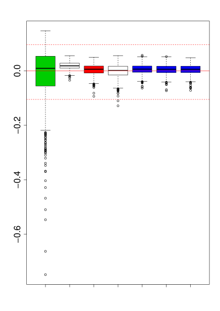
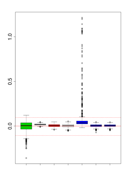
Figure 1: Sampling distribution of $\log\hat{h}/h_{n0}$, with $\hat{h}$ denoting the leave-one-out cross-validation (green) and the bagged bandwidths for different values of $m$. For the bagged bandwidths, we considered $N=500$ and $m\in\{5,000,13,081$ (red)$,20,000,\hat{m}_{0}$ (blue)$\}$, for density D1 (left panel); and $m\in\{5,000,20,326$ (red)$,25,000,\hat{m}_{0}$ (blue)$\}$, for density D2 (right panel). The two white boxes correspond, from left to right, to $m=5,000$ and $20,000$, for D1 (left panel); and to $m=5,000$ and $25,000$, for D2 (right panel). The three blue boxes correspond, from left to right, to $r=500,1,000,5,000$. Red dotted lines are plotted at values 0.9 and 1.1 for reference.

The mean squared error of the bagged bandwidth using $m=\hat{m}_{0}$ may be larger than the one for leave-one-out cross-validation for density D2 using $r=500$, as it can be observed in the left blue box-plot on the right panel in Figure 1. These results are somewhat misleading because the final behaviour of the kernel density estimator with the bagged bandwidth selector, denoted by $\hat{h}$ for simplicity, is still very good in this setting. The distribution of $\hat{h}$ is biased upward and there are numerous extremely large values of $\hat{h}$. However, it turns out that even the largest of these bandwidths produces very effective density estimates, as observed in Figure 2. Consider, for example, $\log\hat{h}/h_{n0}=1$, which means that $\hat{h}\simeq 2.72h_{n0}$. In Figure 2, we provide the claw density and two kernel estimates from a sample of size $10^{5}$. The bandwidths of the two estimates are $h_{n0}=0.031$ and $2.72h_{n0}\simeq 0.084$. The kernel estimate with larger bandwidth captures the five modes and has better tail behaviour than the estimate based on the MISE bandwidth. Figure 2 illustrates the fact that integrated squared error (ISE) loss is not always ideal. One might well prefer an estimate with larger than optimum ISE, as long as it captures all the important features of the underlying density and is smoother than the ISE optimal estimate. However, despite this remark, ISE error criterion can be used to see the effect of the different bandwidth selectors on the kernel density estimates. Figure 3 shows the sampling distribution of ratio of the ISE of the kernel density estimates using the bagging cross-validation bandwidths and the classical cross-validation one, ${\rm ISE}\{\hat{h}(m,N)\}/{\rm ISE}(\hat{h}_{n})$, for both models and the same values of $m$ considered in Figure 1. In this case, outliers were omitted in order to be able to appreciate the differences between the different box-plots.

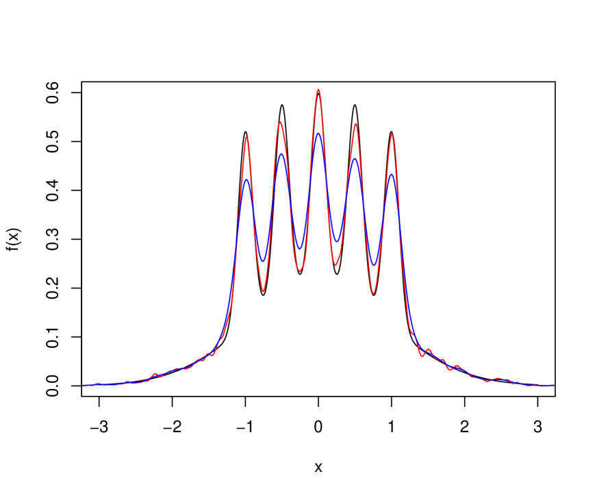
Figure 2: Claw density (black line) and kernel estimates (red and blue lines). The kernel estimates are computed from a sample of size $10^{5}$. The red estimate uses the MISE optimal bandwidth of 0.031 and the blue uses bandwidth $0.084$.

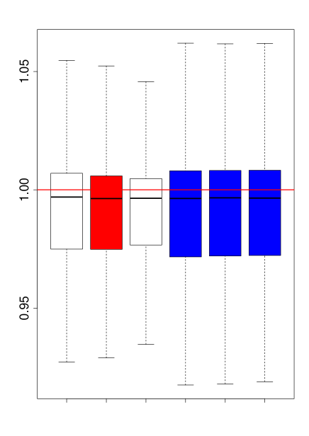
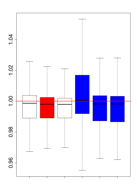
Figure 3: Sampling distribution of the random variable ${\rm ISE}\{\hat{h}(m,N)\}/{\rm ISE}(\hat{h}_{n})$, with $\hat{h}(m,N)$ denoting the bagged bandwidths for different values of $m$, and $\hat{h}_{n}$ denoting the leave-one-out cross-validation bandwidth. For the bagged bandwidths, we considered $N=500$ and $m\in\{5,000,13,081$ (red)$,20,000,\hat{m}_{0}$ (blue)$\}$, for density D1 (left panel); and $m\in\{5,000,20,326$ (red)$,25,000,\hat{m}_{0}$ (blue)$\}$, for density D2 (right panel). The two white boxes correspond, from left to right, to $m=5,000$ and $20,000$, for D1 (left panel); and to $m=5,000$ and $25,000$, for D2 (right panel). The three blue boxes correspond, from left to right, to $r=500,1,000,5,000$.

The means of ${\rm ISE}\{\hat{h}(m,N)\}/{\rm ISE}(\hat{h}_{n})$ for the values of $m$ and $N$, and densities considered in Figure 3, as well as the proportion of times where the ISE of the kernel density estimates using $\hat{h}(m,N)$ is lower than using $\hat{h}_{n}$ are shown in Table 3. In general, it can be observed a slightly better performance of the estimators when using the bagged bandwidths than when employing the leave-one-out cross-validation selector, except when considering the density D2 and using $m=\hat{m}_{0}$, with $r=500$ (left blue box-plot on the right panel in Figure 3). These results are totally consistent with those shown in Figure 1 for the bandwidths.

Table 3: Top Table: means of ${\rm ISE}\{\hat{h}(m,N)\}/{\rm ISE}(\hat{h}_{n})$, with $\hat{h}(m,N)$ computed using the combinations of $m$ and $N$ and densities considered in Figure 3. Bottom Table: proportion of values of $\hat{h}(m,N)$ whose ISE is lower than that of $\hat{h}_{n}$.

			Means
Density	$B_{1}$	$B_{2}$	$B_{3}$	$B_{4}$	$B_{5}$	$B_{6}$
D1	$0.98533$	$0.98505$	$0.98512$	$0.98448$	$0.98428$	$0.98537$
D2	$0.99624$	$0.99594$	$0.99530$	$1.23742$	$0.99539$	$0.99494$
			Proportions
Density	$B_{1}$	$B_{2}$	$B_{3}$	$B_{4}$	$B_{5}$	$B_{6}$
D1	0.606	0.603	0.609	0.590	0.593	0.590
D2	0.584	0.622	0.637	0.461	0.604	0.599

• $B_{i}$ refers to the $i$th box-plot in order of appearance in Figure 3.

In Figure 4, the sampling distribution of $\hat{m}_{0}/m_{0}$ is shown. It can be observed that the mean squared error of $\hat{m}_{0}$ is reduced as $r$ increases. Furthermore, the bias of the estimator depends on the complexity of the target density. For small values of $r$, in spite of the high variability of $\hat{m}_{0}$, the sampling distribution of the bagged bandwidth, considering $m=\hat{m}_{0}$, is virtually unchanged with respect to the case $m=m_{0}$ for densities that are not very complex, such as D1. For more complex densities, such as D2, the effect that the variability of $\hat{m}_{0}$ has on the bagged bandwidth is more noticeable for small values of $r$, translating into a more biased bandwidth. More importantly, when we compare the errors in Figure 4 and Figure 1, it is clear that there is a large range of values for $m$ around its optimal value, $m_{0}$, such that the effect the error of $\hat{m}_{0}$ has on the sampling distribution of $\hat{h}(\hat{m}_{0},N)$ is very small.

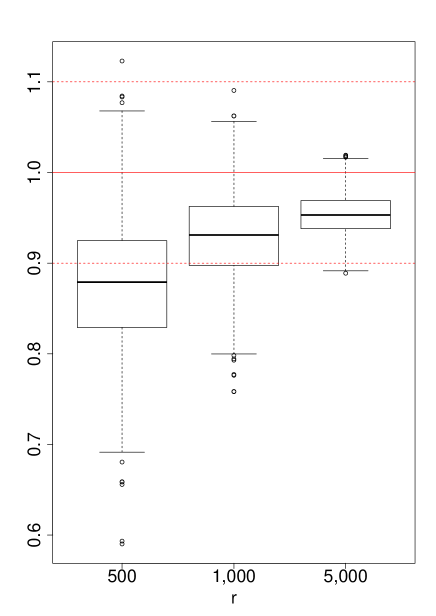
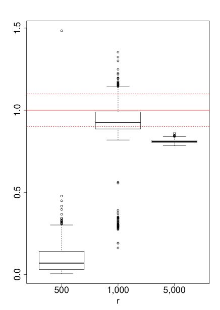
Figure 4: Sampling distribution of $\hat{m}_{0}/m_{0}$, with $\hat{m}_{0}$ denoting the estimator of the optimal subsample size, $m_{0}$, as defined in Section $4$ of the main paper, for densities D1 (left panel) and D2 (right panel). The values chosen for the parameters of the estimator were $s=50$ and, from left to right, $r\in\{500,1,000,5,000\}$. Red dotted lines are plotted at values 0.9 and 1.1 for reference.

Appendix 3. Real data example

To further explore the performance of the bagged bandwidth selector, we considered the public dataset “On-Time: Reporting Carrier On-Time Performance” corresponding to the year $2017$, available at https://www.transtats.bts.gov/Fields.asp. In particular, we were interested in the variable ArrDelay, which measures the difference in minutes between scheduled and actual arrival time. Early arrivals show negative numbers. Due to the fact that the dataset contains many ties and in order to avoid problems when performing cross-validation, we decided to remove the ties by jittering the data. In particular, we worked with the sample of size $n=5,579,346$ which results from adding a random sample of size $n$, drawn from a continuous uniform distribution defined on the interval $(-0.5,0.5)$, to the original dataset.

To estimate the optimal subsample size, $m_{0}$, for the bagged bandwidth, we used the procedure described in Section $4$ of the main paper, considering $N=100$ subsamples. In particular, using $r=1,000$ and $s=500$, yielded the estimate $\hat{m}_{0}=272,222$. The process of estimating $m_{0}$ with those parameters took $32$ seconds. The estimated bagged bandwidth with these values of $m$ and $N$ was $\hat{h}(m=272,222,N=100)=0.490$. Its calculation took $63$ seconds. The calculation of both $\hat{m}_{0}$ and $\hat{h}(m,N)$ were executed in parallel on an Intel Core i5-8600K 3.6GHz. Figure 5 shows the kernel density estimates obtained when considering the bagged bandwidth $h=\hat{h}(\hat{m}_{0},N=100)=0.490$ and the bandwidth produced by the R function bw.ucv, using the same number of bins and search interval as in the case of the bagged bandwidth, that is, $h=$ bw.ucv($\cdot$, nb=1e5, lower=0.01, upper=1), that returned the value 0.01039. As we can see, even with those parameters, bw.ucv basically returns the lower bound of the search interval thus producing a heavily undersmoothed estimate of the underlying density.

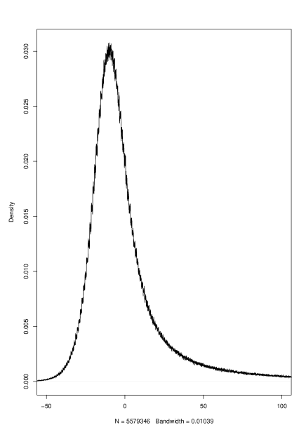
Figure 5: Kernel density estimates with bandwidths $h=\hat{h}(\hat{m}_{0},N=100)$ (left) and $h=$ bw.ucv($\cdot$, nb=1e5, lower=0.01, upper=1) (right).

Computing the leave-one-out cross-validation bandwidth for the whole sample is prohibitive due to the huge amount of time it would require. Even with a binned implementation, as employed in the R function bw.ucv, the computing time would be very high, as highlighted in Section $2$. In order for this function to produce accurate results the number of bins must be very close to $n$. Therefore, to predict the value of the cross-validation bandwidth for the original sample size, $n$, and also the time required for its computation, we used appropriate regression models. We repeated these experiments considering binned and non-binned cross-validation bandwidths. The predicted cross-validation bandwidth for the whole sample is practically identical whether or not one uses binning, with a large enough number of bins, and hence we just describe the experiment when using a binned implementation. Nevertheless, the predicted time is obviously much higher when binning is not used, as we will see later. Specifically, we selected 100 subsamples of sizes $557$, $5,579$ and $55,793$ from the whole dataset. For each size and subsample, we computed the binned version of the leave-one-out cross-validation bandwidth, using the R function bw.ucv with nb, number of bins, equal to the corresponding sample size (see Figure 6). Finally, we considered the parametric regression model:

$$Y_{i}=\beta_{0}n_{i}^{\beta_{1}},$$ (25)

where $n_{i}\in\{557,\,5,579,\,55,793\}$ and $Y_{i}\in\{3.606,2.129,1.352\}$ denotes the mean of the binned cross-validation bandwidths using the subsamples of size $n_{i}$. Taking logarithms in (25), we get a linearized version of (25),

$$\log Y_{i}=\log\beta_{0}+\beta_{1}\log n_{i},$$ (26)

which we can see as a linear regression model with parameters $\log\beta_{0}$, intercept, and $\beta_{1}$, slope. Applying least squares, we obtained the following estimates for the parameters of model (25):

$$\hat{\beta}_{0} = 13.69,$$

$$\hat{\beta}_{1} = -0.213.$$

With these values of $\hat{\beta}_{0}$ and $\hat{\beta}_{1}$, the predicted value of the leave-one-out cross-validation bandwidth for the original sample size is $\hat{h}_{n}=0.501$, very close to the value produced by the bagged approach, $\hat{h}(m=272,222,N=100)=0.490$. Figure 7 shows the fitted values for the nonlinear model defined in (25). Analogously, we considered a model similar to the one described in (25) to predict the time required to compute a binned version of the ordinary cross-validation bandwidth for the original sample. Fitted values for this model are shown in Figure 8. As previosuly, we employed the R function bw.ucv with nb equal to the corresponding sample size to compute the different cross-validation bandwidths. In this case and using the same notation as in (25), we considered $n_{i}=\{5,579,\,55,793,\,557,934\}$ and $Y_{i}=\{0.0102,0.959,103.08\}$, with $Y_{i}$ now denoting the elapsed time (in seconds) needed to compute bw.ucv($\cdot$, nb=$n_{i}$), that is, the binned cross-validation bandwidth for a sample of size $n_{i}$ with the number of bins set to $n_{i}$. Again, using the same notation as in (25), we obtained the following estimates for the model parameters:

$$\hat{\beta}_{0} = 3.14\times 10^{-10},$$

$$\hat{\beta}_{1} = 2.002.$$

This means that the time needed to compute the binned cross-validation bandwidth for the original sample is predicted to be approximately $2.8$ hours. Analogously, we repeated the experiment to predict the time required to compute a non-binned leave-one-out cross-validation bandwidth for the whole sample and this predicted time turned out to be $5.1$ years. Fitted values for the model are shown in Figure 9.

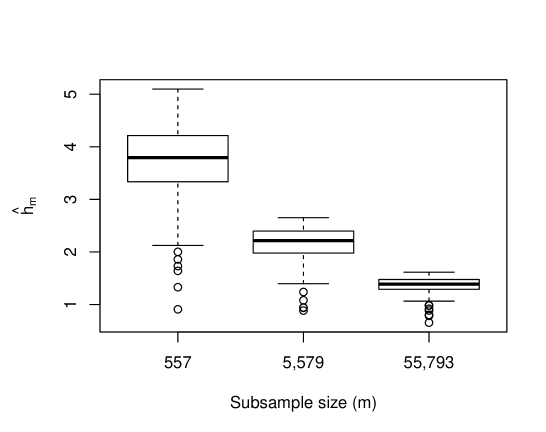
Figure 6: Box-plots of $\hat{h}_{m}$ for subsamples of size $m\in\{557,\,5,579,\,55,793\}$.

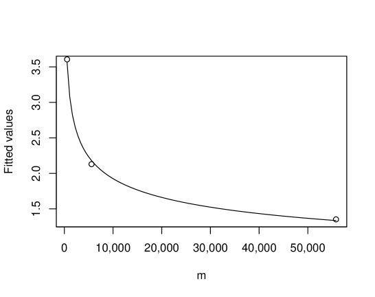
Figure 7: Fitted values for the regression model defined in (25). White dots correspond to the observations used to fit the model.

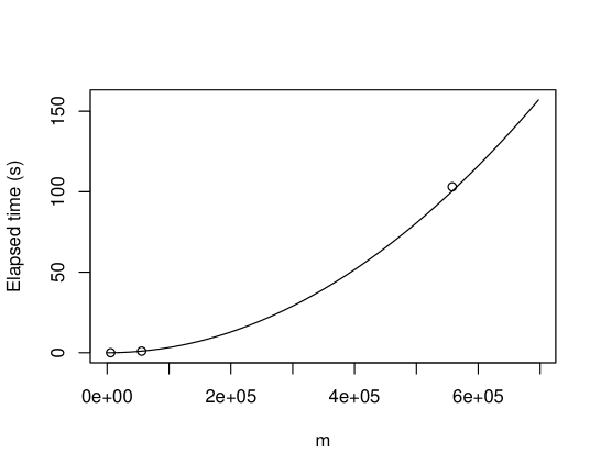
Figure 8: Fitted values for the regression model that relates the elapsed time needed to compute the binned cross-validation bandwidth to the sample size. White dots correspond to the observations used to fit the model.

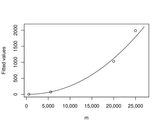
Figure 9: Fitted values for the regression model that relates the elapsed time needed to compute the standard non-binned cross-validation bandwidth to the sample size. White dots correspond to the observations used to fit the model.

Appendix 4. Variance of the bagged bandwidth (Hall and Robinson, 2009)

In this section, we show that the variance approximation of the bagged bandwidth studied in Hall & Robinson (2009) is in error. We also provide the correct expression for this variance and the corresponding proof. The bagged bandwidth studied in Hall & Robinson (2009), $\hat{h}_{bagg}$, corresponds to the case where $N=\infty$ in the smoothing parameter (3) of the main paper, that is, $\hat{h}_{bagg}=\hat{h}(m,\infty)$, following the notation adopted. From equation (7) in the main paper, it follows that

$${\rm var}\left(\hat{h}_{bagg}\right)=AC^{2}m^{9/5}n^{-12/5}+o\left(m^{9/5}n^{-12/5}\right),$$ (27)

which exactly matches the second term given in equation (13) of Hall & Robinson (2009). However, it is claimed in that paper that the dominant term is of order $m^{4/5}n^{-7/5}$. We will prove that this last statement is wrong and that, in fact, the dominant term is precisely the one given in (27).

It can be easily proved that for a sample of size $n$ we have

$$CV(h)=M(h)-R(f)+S(h),$$ (28)

where, as previously, $M(h)$ denotes the MISE function of the Parzen–Rosenblatt kernel density estimator for a sample of size $n$, and $S(h)=S_{1}(h)+S_{2}(h)$ is defined on p. $184$ of Hall & Robinson (2009). From (28) it follows that, for any $r\in\mathbb{N}$,

$${\rm var}\left\{CV^{(r)}(h)\right\}={\rm var}\left\{S^{(r)}(h)\right\}.$$

More importantly, finding the asymptotic variance of the cross-validation bandwidth, whether bagged or ordinary, boils down to finding ${\rm var}\left\{S^{\prime}(h)\right\}$. As stated in equation (14) in Section Appendix 1. Theoretical results of this document, for any $r\geq 1$,

$$CV^{(r)}(h)=M^{(r)}(h)+\frac{1}{n(n-1)}\sum\limits_{i\neq j}\bar{\gamma}_{nh}^{(r)}(X_{i}-X_{j}),$$

where

$$\bar{\gamma}_{nh}^{(r)}(u)=\gamma_{nh}^{(r)}(u)-E\left\{\gamma_{nh}^{(r)}(X_{1}-X_{2})\right\},$$

$$\gamma_{nh}^{(r)}(u)=\frac{{\rm d}^{r}\gamma_{nh}(u)}{{\rm d}h^{r}},$$

$$\gamma_{nh}(u)=\gamma_{n}(u/h)/h$$

and

$$\gamma_{n}(u)=\frac{n-1}{n}K*K(u)-2K(u).$$

Therefore,

$${\rm var}\left\{S^{\prime}(h)\right\}=\frac{1}{n^{4}h^{2}}{\rm var}\left\{\sum\limits_{i\neq j}H(X_{i}-X_{j})\right\},$$ (29)

where

$$H(u)=\gamma_{e,h}(u)+u(\gamma_{e,h})^{\prime}(u),$$

$$\gamma_{e,h}(u)=\gamma_{e}(u/h)/h$$

and

$$\gamma_{e}(u)=\frac{n}{n-1}\gamma_{n}(u).$$

Let us now define $\tilde{H}(u)=\gamma_{e}(u)+u\gamma_{e}^{\prime}(u)$, so we have that $H(u)=\tilde{H}_{h}(u)$. Standard algebra gives

$${\rm var}\left\{\sum\limits_{i\neq j}H(X_{i}-X_{j})\right\}=4n(n-1)(n-2)C_{b}+2n(n-1)C_{c},$$ (30)

where $C_{b}={\rm cov}\left\{H(X_{1}-X_{2}),H(X_{1}-X_{3})\right\}$ and $C_{c}={\rm var}\left\{H(X_{1}-X_{2})\right\}$. These terms can be further decomposed into

$$C_{b}=C_{b1}-C_{b2}^{2}$$ (31)

and

$$C_{c}=C_{c1}-C_{b2}^{2},$$ (32)

where

$$C_{b1} = \int H*f(x)^{2}f(x)\,{\rm d}x,$$

$$C_{c1} = \int H^{2}*f(x)f(x)\,{\rm d}x,$$

$$C_{b2} = \int H*f(x)f(x)\,{\rm d}x.$$

Using the facts that $\tilde{H}$ is symmetric, $\mu_{0}\left(\tilde{H}\right)=0$, $\mu_{2}\left(\tilde{H}\right)=4\mu_{2}(K)/(n-1)$, and $\mu_{4}\left(\tilde{H}\right)=\mu_{6}\left(\tilde{H}\right)=O\left(1\right)$, we have

$$C_{b2} = \int\int\frac{1}{h}\tilde{H}\left(\frac{x-y}{h}\right)f(y)f(x)\,{\rm d}x\,{\rm d}y=\int\int\tilde{H}(u)f(x-hu)f(x)\,{\rm d}x\,\rm{d}u$$

$$= \int\int\tilde{H}(u)\left\{f(x)-huf^{\prime}(x)+\cdots-\frac{h^{5}u^{5}}{5!}f^{(5)}(x)+\frac{h^{6}u^{6}}{6!}f^{(6)}(\tilde{x})\right\}f(x)\,{\rm d}x\,{\rm d}u$$

$$= \int f(x)\left\{\frac{h^{2}}{2}\mu_{2}\left(\tilde{H}\right)f^{\prime\prime}(x)+\frac{h^{4}}{4!}\mu_{4}\left(\tilde{H}\right)f^{(4)}(x)+O\left(h^{6}\right)\right\}\,{\rm d}x$$

$$= \frac{1}{4}\mu_{2}(K)^{2}R(f^{\prime\prime})h^{4}+O\left(h^{6}\right),$$

and, therefore,

$$C_{b2}^{2}=\frac{1}{16}\mu_{2}(K)^{4}R(f^{\prime\prime})^{2}h^{8}+O\left(h^{10}\right).$$ (33)

For the term $C_{b1}$,

$$C_{b1} = \int f(x)\left\{\int\frac{1}{h}\tilde{H}\left(\frac{x-y}{h}\right)f(y)\,dy\right\}^{2}\,{\rm d}x=\int f(x)\left\{\int\tilde{H}(u)f(x-hu)\,du\right\}^{2}\,{\rm d}x$$ (34)

$$= \int f(x)\left\{\frac{1}{4}\mu_{2}(K)^{2}f^{(4)}(x)h^{4}+O\left(h^{6}\right)\right\}^{2}\,{\rm d}x$$

$$= \int f(x)\left\{\frac{1}{16}\mu_{2}(K)^{4}f^{(4)}(x)^{2}h^{8}+O\left(h^{10}\right)\right\}\,{\rm d}x$$

$$= \frac{1}{16}\mu_{2}(K)^{4}J_{1}h^{8}+O\left(h^{10}\right),$$

where

$$J_{1}=\int f^{(4)}(x)^{2}f(x)\,{\rm d}x.$$

The term $C_{b1}$ can be handled in a similar way

$$C_{c1} = \frac{1}{h^{2}}\int\int\tilde{H}\left(\frac{x-y}{h}\right)^{2}f(y)f(x)\,{\rm d}x\,{\rm d}y=\frac{1}{h}\int\int\tilde{H}(u)^{2}f(x-hu)f(x)\,{\rm d}x\,{\rm d}u$$ (35)

$$= \frac{1}{h}\int\int\tilde{H}(u)^{2}f(x)\left\{f(x)-huf^{\prime}(x)+\frac{h^{2}u^{2}}{2}f^{\prime\prime}(\tilde{x})\right\}\,{\rm d}x\,{\rm d}u$$

$$= \frac{R(f)R\left(\tilde{H}\right)}{h}+O\left(h\right).$$

Plugging (33), (34) and (35) into (31) and (32) yields, respectively,

$$C_{b}=\frac{1}{16}\mu_{2}(K)^{4}\left\{J_{1}-R(f^{\prime\prime})^{2}\right\}h^{8}+O\left(h^{10}\right),$$ (36)

$$C_{c}=\frac{R(f)R\left(\tilde{H}\right)}{h}+O\left(h\right).$$ (37)

Now, plugging (36) and (37) into (30) and then into (29), and using the fact that $2R\left(f\right)R\left(\tilde{H}\right)=A_{3}+O\left(n^{-1}\right)$, we get

$${\rm var}\left\{S^{\prime}(h)\right\}=A_{3}\frac{1}{n^{2}h^{3}}+O\left(\frac{1}{n^{2}h}\right),$$ (38)

where $A_{3}$ is defined on p. 183 of Hall & Robinson (2009). Equation (38) is completely consistent with the results obtained in Hall & Marron (1987) and Scott & Terrell (1987). Now, taking variance in equation (A2) of Hall & Robinson (2009) and plugging (38) into that expression yields (27). Equation (38) is enough to show that expression (A3) of Hall & Robinson (2009) is wrong, which in turn explains the error in their equation (13) regarding the variance of the bagged bandwidth. Nonetheless, we will provide an asymptotic expression for ${\rm var}\left\{S_{1}^{\prime}(h)\right\}$, since that is where the error in Hall & Robinson (2009) comes from.

From the definition of $V_{nh}(X_{i})$ and $S_{1}(h)$ given on p. 184 of Hall & Robinson (2009), it is easy to show that

$$V_{nh}(X_{1})=\left(1-n^{-1}\right)\tilde{z}_{1}^{(h)}-\tilde{T}_{1}^{(h)},$$

where

$$\tilde{z}_{1}^{(h)}=K_{h}*K_{h}*f(X_{1})-\int K_{h}*f(x)^{2}\,{\rm d}x$$

and

$$\tilde{T}_{1}^{(h)}=2\left\{K_{h}*f(X_{1})-\int K_{h}*f(x)f(x)\,{\rm d}x\right\}.$$

Let us define the functions $\nu$ and $\eta$, where

$$\nu(x)=K(x)+xK(x)$$

and

$$\eta(x)=K*K(x)+x(K*K)^{\prime}(x).$$

Then, we have that

$$\frac{{\rm d}\tilde{T}_{1}^{(h)}}{{\rm d}h}=-\frac{1}{h}\nu_{h}*f(X_{1})$$

and

$$\frac{{\rm d}\tilde{z}_{1}^{(h)}}{{\rm d}h}=-\frac{1}{h}\left[\eta_{h}*f(X_{1})-\mbox{E}\left\{\eta_{h}*f(X_{1})\right\}\right].$$

Therefore,

$$\frac{{\rm d}V_{nh}(X_{1})}{{\rm d}h}=\frac{1}{h}\left[\tau_{h}*f(X_{1})-\mbox{E}\left\{\tau_{h}*f(X_{1})\right\}\right],$$

where

$$\tau(x)=2K(x)+2xK^{\prime}(x)-\frac{n-1}{n}\left\{K*K(x)+x(K*K)^{\prime}(x)\right\}.$$

We have that

$${\rm var}\left\{\frac{{\rm d}V_{nh}(X_{1})}{{\rm d}h}\right\}=\frac{1}{h}\left[\mbox{E}\left\{\tau_{h}*f(X_{1})^{2}\right\}-\mbox{E}\left\{\tau_{h}*f(X_{1})\right\}^{2}\right].$$

It is easy to show that

$$\mu_{0}(\tau) = 0,$$

$$\mu_{2}(\tau) = -\frac{4}{n}\mu_{2}(K),$$

$$\mu_{4}(\tau) = -\frac{8}{n}\mu_{4}(K)+24\frac{n-1}{n}\mu_{2}(K)^{2},$$

$$\mu_{6}(\tau) = -\frac{12}{n}\mu_{6}(K)+180\frac{n-1}{n}\mu_{2}(K)\mu_{4}(K).$$

Using standard calculations, one can see that

$$\mbox{E}\left\{\tau_{h}*f(X_{1})\right\} = \int\int\tau(u)f(x)f(x-hu)\,{\rm d}x\,{\rm d}u$$

$$= \int\int\tau(u)f(x)\left\{f(x)-huf^{\prime}(x)+\cdots-\frac{h^{7}u^{7}}{7!}f^{(7)}(x)+\frac{h^{8}u^{8}}{8!}f^{(8)}(\tilde{x})\right\}\,{\rm d}x\,{\rm d}u$$

$$= -\frac{h^{2}}{2}\mu_{2}(\tau)R(f^{\prime})+\frac{h^{4}}{24}\mu_{4}(\tau)R(f^{\prime\prime})-\frac{h^{6}}{6!}\mu_{6}(\tau)R(f^{\prime\prime\prime})+O\left(h^{8}\right).$$

Therefore,

$$\mbox{E}\left\{\tau_{h}*f(X_{1})\right\}^{2} = \frac{h^{4}}{4}\mu_{2}(\tau)^{2}R(f^{\prime})^{2}-\frac{h^{6}}{24}\mu_{2}(\tau)\mu_{4}(\tau)R(f^{\prime})R(f^{\prime\prime})$$

$$+ \frac{h^{8}}{24^{2}}\mu_{4}(\tau)^{2}R(f^{\prime\prime})^{2}+\frac{h^{8}}{6!}\mu_{2}(\tau)\mu_{6}(\tau)R(f^{\prime})R(f^{\prime\prime\prime})+O\left(h^{10}\right).$$

On the other hand,

$$\mbox{E}\left\{\tau_{h}*f(X_{1})^{2}\right\} = \int\int\int\tau(u)f(x-hu)\tau(v)f(x-hv)f(x)\,{\rm d}x\,{\rm d}u\,{\rm d}v$$

$$= \int\int\int\tau(u)\tau(v)f(x)\left\{f(x)-huf^{\prime}(x)+\cdots+O\left(h^{10}\right)\right\}$$

$$\left\{f(x)-hvf^{\prime}(x)+\cdots+O\left(h^{10}\right)\right\}\,{\rm d}x\,{\rm d}u\,{\rm d}v$$

$$= \frac{h^{4}}{4}\mu_{2}(\tau)^{2}J_{2}+\frac{h^{6}}{24}\mu_{2}(\tau)\mu_{4}(\tau)J_{3}+\frac{h^{8}}{6!}\mu_{2}(\tau)\mu_{6}(\tau)J_{4}+\frac{h^{8}}{24^{2}}\mu_{4}(\tau)^{2}J_{1}+O\left(h^{10}\right),$$

where

$$J_{2} = \int f(x)f^{\prime\prime}(x)^{2}\,{\rm d}x,$$

$$J_{3} = \int f(x)f^{\prime\prime}(x)f^{(4)}(x)\,{\rm d}x,$$

$$J_{4} = \int f(x)f^{\prime\prime}(x)f^{(6)}(x)\,{\rm d}x.$$

So, we have that

$${\rm var}\left\{\frac{{\rm d}V_{nh}(X_{1})}{{\rm d}h}\right\} = \frac{h^{2}}{4}\mu_{2}(\tau)^{2}\left\{J_{2}-R(f^{\prime})^{2}\right\}+\frac{h^{4}}{24}\mu_{2}(\tau)\mu_{4}(\tau)\left\{J_{3}+R(f^{\prime})R(f^{\prime\prime})\right\}$$

$$+ \frac{h^{6}}{6!}\mu_{2}(\tau)\mu_{6}(\tau)\left\{J_{4}-R(f^{\prime})R(f^{\prime\prime\prime})\right\}$$

$$+ \frac{h^{6}}{24^{2}}\mu_{4}(\tau)^{2}\left\{J_{1}-R(f^{\prime\prime})^{2}\right\}+O\left(h^{8}\right).$$

Finally, since

$${\rm var}\left\{S_{1}^{\prime}(h)\right\}=\frac{4}{n}{\rm var}\left\{\frac{{\rm d}V_{nh}(X_{1})}{{\rm d}h}\right\},$$

it follows that

$${\rm var}\left\{S_{1}^{\prime}(h)\right\}=4\mu_{2}(K)^{4}\left\{J_{1}-R(f^{\prime\prime})^{2}\right\}\frac{h^{6}}{n}+O\left(\frac{h^{8}}{n}\right).$$

This, in conjunction with (38), proves that ${\rm var}\left\{S_{1}^{\prime}(h)\right\}$ is negligible with respect to ${\rm var}\left\{S_{2}^{\prime}(h)\right\}$ and, in particular, that ${\rm var}\left\{S_{1}^{\prime}(h)\right\}$ cannot be asymptotic to $A_{2}\,h^{2}/n$ as claimed in Hall & Robinson (2009).

References

• Barreiro-Ures et al. (2019) Barreiro-Ures, D., Hart, J. D., Cao, R. & Francisco-Fernandez, M. (2019). baggedcv: bagged cross-validation for kernel density bandwidth selection. R package version 1.0. https://cran.r-project.org/package=baggedcv.
• Bhattacharya & Hart (2016) Bhattacharya, A. & Hart, J. D. (2016). Partitioned cross-validation for divide-and conquer density estimation. ArXiv:1609.00065.
• Cao (1993) Cao, R. (1993). Bootstrapping the mean integrated squared error. J. Mult. Anal. 45, 137–160.
• Feluch & Koronacki (1992) Feluch, W. & Koronacki, J. (1992). A note on modified cross-validation in density estimation. Comput. Statist. Data Anal. 13, 143–151.
• Friedman & Hall (2007) Friedman, J. H. & Hall, P. (2007). On bagging and nonlinear estimation. J. Statist. Plan. Infer. 137, 669–683.
• Hall & Marron (1987) Hall, P. & Marron, J. (1987). Extent to which least-squares cross-validation minimises integrated square error in nonparametric density estimation. Prob. Theory Rel. Fields 74, 567–581.
• Hall et al. (1992) Hall, P., Marron, J. & Park, B. (1992). Smoothed cross-validation. Prob. Theory Rel. Fields 92, 1–20.
• Hall & Robinson (2009) Hall, P. & Robinson, A. P. (2009). Reducing variability of crossvalidation for smoothing parameter choice. Biometrika 96, 175–186.
• Hart & Yi (1998) Hart, J. D. & Yi, S. (1998). One-sided cross-validation. J. Am. Statist. Assoc. 93, 620–631.
• Loader (1999) Loader, C. R. (1999). Bandwidth selection: classical or plug-in? Ann. Statist. 27, 415–438.
• Mammen et al. (2011) Mammen, E., Martínez-Miranda, M. D., Nielsen, J. P. & Sperlich, S. (2011). Do-validation for kernel density estimation. J. Am. Statist. Assoc. 106, 651–660.
• Marron (1987) Marron, J. S. (1987). Partitioned cross-validation. Econom. Rev. 6, 271–283.
• Marron & Wand (1992) Marron, J. S. & Wand, M. P. (1992). Exact mean integrated squared error. Ann. Statist. 20, 712–736.
• Miranda et al. (2011) Miranda, M. M., Nielsen, J. & Sperlich, S. (2011). One-sided cross-validation for density estimation with an application to operational risk. In Operational Risk toward Basel III, G. N. Gregoriou, ed., chap. 9. New Jersey: John Wiley & Sons, Ltd, pp. 177–195.
• Park & Marron (1990) Park, B. & Marron, J. S. (1990). Comparsion of data-driven bandwidth selectors. J. Am. Statist. Assoc. 85, 66–72.
• Parzen (1962) Parzen, E. (1962). On estimation of a probability density function and mode. Ann. Math. Statist. 33, 1065–1076.
• R Development Core Team (2020) R Development Core Team (2020). R: A Language and Environment for Statistical Computing. R Foundation for Statistical Computing, Vienna, Austria. http://www.R-project.org.
• Rosenblatt (1956) Rosenblatt, M. (1956). Remarks on some nonparametric estimates of a density function. Ann. Math. Statist. 27, 832–837.
• Savchuk et al. (2010) Savchuk, O., Hart, J. D. & Sheather, S. J. (2010). Indirect cross-validation for density estimation. J. Am. Statist. Assoc. 105, 415–423.
• Scott & Terrell (1987) Scott, D. & Terrell, G. (1987). Biased and unbiased cross-validation in density estimation. J. Am. Statist. Assoc. 82, 1131–1146.
• Scrucca et al. (2016) Scrucca, L., Fop, M., Murphy, T. B. & Raftery, A. E. (2016). mclust 5: clustering, classification and density estimation using Gaussian finite mixture models. R. J. 8, 205–233.
• Serfling (1980) Serfling, R. (1980). Approximation Theorems of Mathematical Statistics. Wiley Series in Probability and Statistics - Applied Probability and Statistics Section Series. Wiley.
• Sheather & Jones (1991) Sheather, S. J. & Jones, M. C. (1991). A reliable data-based bandwidth selection method for kernel density estimation. J. Roy. Statist. Soc. Ser. B 53, 683–690.
• Silverman (1986) Silverman, B. W. (1986). Density Estimation for Statistics and Data Analysis. Monographs on Statistics and Applied Probability. London: Chapman & Hall.
• Stone (1974) Stone, M. (1974). Cross-validatory choice and assessment of statistical predictions. J. R. Statist. Soc. B 36, 111–147.
• Stute (1992) Stute, W. (1992). Modified cross-validation in density estimation. J. Statist. Plan. Infer. 30, 293–305.