Shrub of a thousand faces: an individual segmentation from satellite images using deep learning

Rohaifa Khaldi^a,b,e (rohaifa@go.ugr.es), Siham Tabik^b (siham@ugr.es), Sergio Puertas-Ruiz^f (s.p.r@csic.es), Julio Peñas de Giles^c (jgiles@ugr.es), José Antonio Hódar Correa^c (jhodar@ugr.es), Regino Zamora^d,e (rzamora@ugr.es), Domingo Alcaraz Segura^c,e (dalcaraz@ugr.es)

^a LifeWatch-ERIC, ICT Core, 41071 Seville, Spain.
^b Dept. of Computer Science and Artificial Intelligence, Andalusian Research Institute in Data Science and Computational Intelligence, DaSCI, University of Granada, 18071 Granada, Spain.
^c Department of Botany, Faculty of Science, University of Granada, 18071 Granada, Spain.
^d Department of Ecology, Faculty of Science, University of Granada, 18071 Granada, Spain.
^e Interuniversity Institute of Earth System Research in Andalusia, Andalusian Center for the Environment (IISTA-CEAMA), Granada, 18071, Spain
^f Pyrenean Institute of Ecology, Spanish National Research Council (IPE-CSIC), 50059 Zaragoza, Spain.

Abstract

Monitoring the distribution and size-structure of long-living shrubs, such as Juniperus communis L. (common juniper), can be used to estimate the long-term effects of climate change on high-mountain and high latitude ecosystems. Historical aerial very-high resolution imagery offers a retrospective tool to monitor shrub growth and distribution at high precision. Currently, deep learning models provide impressive results for detecting and delineating the contour of objects with defined shapes. However, adapting these models to detect natural objects that express complex growth patterns, such as junipers, is still a challenging task.

This research presents a novel approach that leverages remotely sensed RGB imagery in conjunction with Mask R-CNN-based instance segmentation models to individually delineate Juniperus shrubs above the treeline in Sierra Nevada (Spain). In this study, we propose a new data construction design that consists in using photo interpreted (PI) and field work (FW) data to respectively develop and externally validate the model. We also propose a new shrub-tailored evaluation algorithm based on a new metric called Multiple Intersections over Ground Truth Area (MIoGTA) to assess and optimize the model shrub-delineation performance. Finally, we deploy the developed model for the first time to generate a wall-to-wall map of Juniperus individuals.

The experimental results demonstrate the efficiency of our dual data construction approach (PI and FW) in overcoming the limitations associated with traditional field survey methods. They also highlight the robustness of our MIoGTA metric in evaluating instance segmentation models on species with complex growth patterns showing more resilience against data annotation uncertainty. Furthermore, they show the effectiveness of employing Mask R-CNN with ResNet101-C4 backbone in delineating PI and FW shrubs, achieving F1-score of 87,87% and 76.86%, respectively. The deployment results reveal that the shrubs are highly concentrated in the North-West region, in the North-West orientation, and within a specific range of slope and altitude. In addition, they show that smaller shrubs tend to currently occur at higher altitudes and larger shrubs at lower altitudes.

1 Introduction

Climate change is forcing species to move latitudinally and altitudinally to maintain their climatic optimum. Species are often moving rapidly over large geographic areas, so methodological tools are needed to track these massive movements over large areas and to identify the dynamics of advancing and retreating fronts. The study of the distribution and abundance of organisms has always been a fundamental tenet in ecological science (Townsend et al. 2003, Krebs 2013). This study can be approached at the regional scale, where the focus is on abundance along the range of each species, from the center of the range to the periphery at latitudinal and altitudinal distribution limits. But it can also be approached from a more local perspective, where the focus is on analyzing the distribution and abundance of each individual and the factors (abiotic and biotic) that determine them at a much finer scales of analysis. Classical field surveys (e.g., transects, plots) to count individuals are the most accurate, but it is impractical to use them when trying to identify and count individuals over vast and frequently remote areas. New methodological tools need to be developed to enable ecologists to identify, count and map individuals over large areas with precision.

High-mountain shrubs play a vital role in ecosystems, contributing significantly to soil stabilization in the headwaters of watersheds, carbon sequestration, wildlife habitat provision, microclimate moderation, and overall biodiversity support (Adhikari et al. 2017). Climate change may intensify the vulnerability of these species, and reshape their geographical ranges to more climatically suitable regions (El-Barougy et al. 2023, Bellard et al. 2012). In this context, the development of high-precision maps at individual level is indispensable for an accurate, but efficient and timely tracking of shrub distribution (Otto et al. 2012, Thompson 2006). This precise but quick mapping is essential for various purposes, including environmental monitoring, biodiversity conservation, forestry, climate impact assessment, invasive species monitoring, land management, and urban planning (Ayhan et al. 2020).

Monitoring the distribution and size-structure of Juniperus communis L. (common juniper) could be used to estimate the long-term effects of climate change on high-mountain and high latitude ecosystems throughout the northern hemisphere. The common juniper is one of the most widely-spread woody plants of the world and it is frequently one of the last species that conform the woody-line in high latitudes and mountains. However, these situations often occur in remote locations and in complex terrains, posing a challenge for both field surveys and remote sensing.

Combining remote sensing (RS) and artificial intelligence (AI) technologies can provide a great opportunity to improve in-situ field surveying by opening up opportunities for automation. Remote sensing technologies offer highly detailed spatial resolution granting exceptional flexibility in data acquisition (Zhang et al. 2020). This data can be afterwards processed by deep learning (DL) technologies for automatic identification of shrubs.

Many studies have used remote sensing data to generate land cover maps including shrublands (Niphadkar et al. 2017, Ayhan & Kwan 2020, Soubry et al. 2022). These studies have been performed to capture a broad distribution of shrubs without delineating individually a specific type of shrub. Only a few attempts have been made to identify individuals of a particular species of shrub. So far and for the best of our knowledge, all the studies that have used machine learning (ML) models and DL models to detect shrub individuals using remote sensing data are summarized in Table 1. According to these studies, three remote sensing technologies have been used to perform this operation. The most common one is UAV (Unmanned Aerial Vehicle), followed by Google Earth (GE) satellite, then LiDAR (Light Detection and Ranging). Initially GE satellite data was used by Guirado et al. (2017) to detect Ziziphus lotus shrubs using patch-based classification approach. Then, different studies appeared using aerial photography which captures very-high resolution images of shrubs, and facilitates the process of shrub detection (James & Bradshaw 2020, Li et al. 2021, James & Bradshaw 2021, Retallack et al. 2022). Further, another attempt combining both UAV and GE satellite data was applied by Guirado et al. (2021) to perform instance segmentation of Ziziphus lotus shrubs. Eventually, another study used LiDAR with laser technology to collect volumetric data to make three-dimensional detection of Cytisus scoparius shrubs (Madsen et al. 2020). While LiDAR and UAVs offer higher spatial resolution and flexibility for data collection, satellites provide large-scale coverage, long-term monitoring capabilities, and cost-effectiveness.

These investigations are each constrained by various limitations. (1) It is important to highlight that all the existing studies have been conducted across three distinct ecosystems, primarily encompassing the arid landscapes of Australia, China, and Spain, as well as the grasslands of Denmark, and the fynbos biome in South Africa. Mountain areas have never been tackled. (2) It is noteworthy to mention that only one study has utilized satellite data for the purpose of shrub delineation (Guirado et al. 2021). (3) It is essential to stress that all the studied shrubs have an easy growth patterns (i.e., scattered distributions, homogeneous shapes, fixed sizes and colors, etc.) which to some extent, make their detection/delineation process more straightforward. (4) Eventually, none of these studies have deployed the model to generate a large scale distribution map of these shrubs.

Table 1: Review of studies using remote sensing and machine/deep learning to identify shrub individuals.

Shrub species	RS technology	Spatial resolution	Data type	Data size	Open source	Mapping approach	Model	Study area	Ecosystem type	Reference
Hakea suaveolens and Hakea sericea	UAV	20 cm	RGB	100 images with shrubs	No	Semantic segmentation	U-Net	South Africa	Fynbos	James & Bradshaw (2020)
4 species	UAV	1.5 cm	RGB	2991 shrubs	No	Semantic segmentation	OBIA + Random Forest	Northwest China	Dryland	Li et al. (2021)
Hakea sericea	UAV	-	RGB	100 images with shrubs	No	Patch-based classification and Semantic segmentation	Xception Inception MobileNet U-Net	South Africa	Fynbos	James & Bradshaw (2021)
pearl bluebush and Maireana sedifolia	UAV	(0.8, 2, 3) cm	RGB	4111 shrubs	No	Object detection	Faster-RCNN YOLO-V3 SSD	South of Australia	Dryland	Retallack et al. (2022)
Cytisus scoparius	LiDAR	2 cm	Structural features	65 shrubs	No	3D point detection	Machine learning models	Denmark	Grassland	Madsen et al. (2020)
Ziziphus lotus (scattered shrubs)	GE satellite	12 cm	RGB	82 shrubs	No	Patch-based classification	GoogleNet and ResNet	South of Spain and Cyprus	Dryland	Guirado et al. (2017)
Ziziphus lotus (scattered shrubs)	GE satellite and UAV	1m	RGB	-	Under request	Instance segmentation	Mask R-CNN + OBIA	South of Spain	Dryland	Guirado et al. (2021)
Juniperus	GE Satellite	13 cm	RGB	8580 shrubs	Yes	Instance segmentation	Mask R-CNN	South of Spain	High-mountain	Ours

In general, shrub delineation using Convolution Neural Networks (CNNs) can be effective when these shrubs have a consistent pattern in size, color, shape, density, and the scene is relatively simple. However, this process may become more challenging in scenarios with multiple faces shrubs (i.e., shrubs with complex growth patterns) and complex backgrounds such as areas where shrubs and trees grow together, different species coexist, or where there are intricate clusters of individual shrubs (Dong et al. 2019). These scenarios make the field surveying process challenging where most of the time experts face difficulties in recognizing the real extent of these shrubs. This complexity in input data affects the data annotation process leading to various issues. These include incorrect detections, known as False Positives (FPs), and overlooked detections, referred to as False Negatives (FNs). The data annotation task becomes increasingly challenging, less certain, and generally less uniform. Sometimes, a cluster of individuals may be perceived by experts as a single entity, while at other times, it might be identified as multiple entities. Additionally, experts often encounter challenges in accurately delineating specific shrub species from others. Subsequently, the data modeling task becomes more critical since it depends on three factors: (1) the data complexity, (2) the results of the data annotation process, and (3) the model performance itself. These factors can lead the model to detect multiple annotated individuals as one individual or one annotated individual as multiple individuals, it may also lead the model to totally ignore some target shrubs or make a partial detection of shrubs. For these reasons, a fair model evaluation process should be applied that takes into consideration the uncertainty associated with data labels.

The research reported in this paper aims to combine AI and RS technologies using a new data construction design and a new model evaluation protocol to individually delineate Juniperus shrubs from RGB satellite images. We used Juniperus shrubs as a proof of concept because it is a species that has a wide latitudinal distribution in Eurasia. These species that colonizes mountains, hold a complex orography that tests the use of remote sensing, whose usefulness is proven in flat scenarios. Thus, having a wide latitudinal and altitudinal distribution, these shrubs become an ideal model species for determining the ability of AI models to detect changes in distribution and abundance resulting from global change at a very fine spatial resolution scale.

Our main contributions are summarized as follows:

• We proposed the largest open-source DL-ready dataset for individual delineation of shrubs.

• We introduced a DL-ready dataset for instance segmentation of plants with complex growth patterns.

• We proposed a new data construction approach to overcome the limitations of field surveying methods.

• We explored the potential of AI models to individually delineate plants with complex growth patterns.

• We proposed a model evaluation protocol for plants with complex growth patterns.

• We generated a wall-to-wall map of high-mountain individual shrubs and counted their numbers.

• We analyzed the distribution of high-mountain shrubs with respect to different topographical features.

The structure of this study is organized as follows: Section 2 describes the study area, the target shrub, and the new data construction design. Section 3 outlines the research methodology used in our study for individual delineation of shrubs. Section 4 presents the obtained results. Section 5 provides a discussion of the methodological and ecological considerations as well as the study limitations. Section 6 summarizes the key findings of the study and sheds light onto future works.

2 Study area and materials

This section describes the study area and provides details about how the dual data construction approach was designed. In this study, we consider the challenging task of delineating a specific type of shrubs in high mountain ecosystem using GE satellite RGB images.

2.1 Study area

This research occurred in the Sierra Nevada National Park located on the southern fringe of Iberia at $37^{o}06^{\prime}$N $3^{o}05^{\prime}$ W, between the provinces of Granada and Almería, Spain (Fig. 1). This park contains the highest mountains in western Europe after the Alps, with an elevation of 3479 m at the Mulhacén peak (Palacios et al. 2020). This ecosystem includes an abundance of two long-living shrubs, named Juniperus communis and Juniperus sabina, with priority conservation interest at the European level.

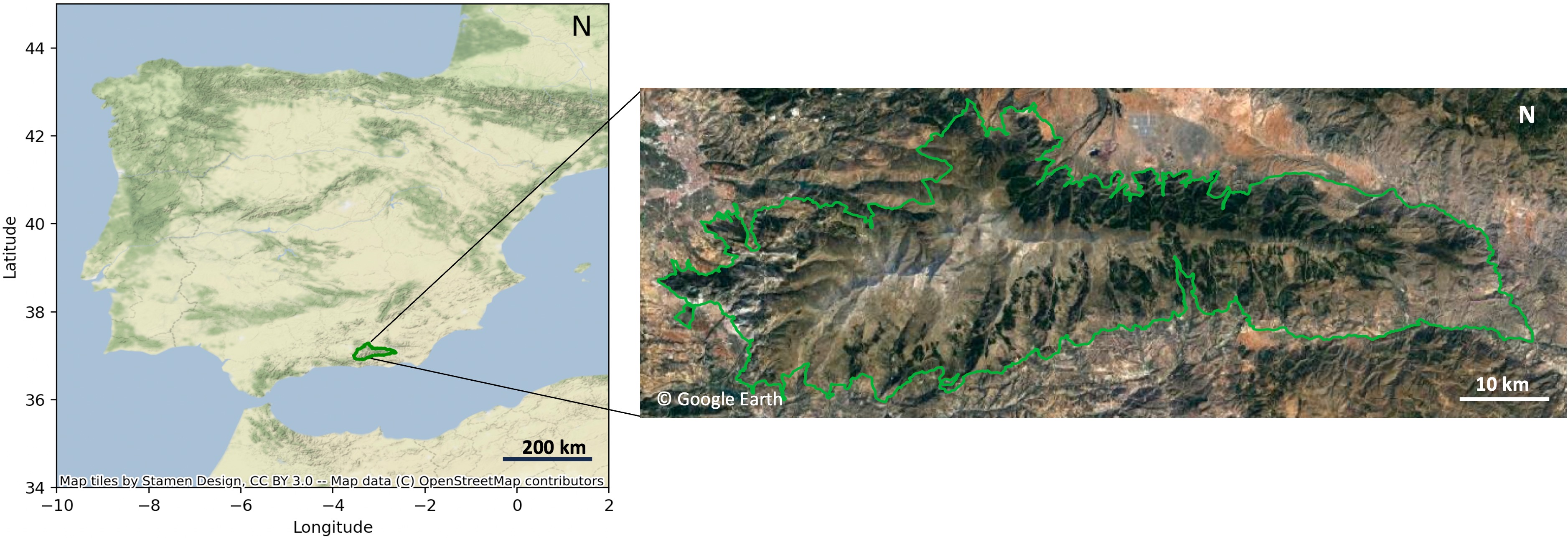
Figure 1: Location of the study area in the National Park of Sierra Nevada (Andalusia, Spain). The green line shows the border of the Natural Park that surrounds the National Park.

2.2 Target species

Common juniper, Juniperus communis L. (Cupresaceae), is among the most widely distributed gymnosperms in the Holarctic, ranging from circum-Mediterranean mountains up to subarctic tundra (García et al. 2000). Juniperus communis is a typical dwarf evergreen needle-leaf long-living shrub that occurs on poor soils and harsh environments. This species shows a continuous distribution in northern and central Europe, but populations become progressively more fragmented towards the Mediterranean Basin, where the species is located exclusively in high-mountain areas, dominating the strip between the tree-line and the woody-line. These populations, such as those in the southern Iberian Peninsula, are characterized by a very low regeneration ability under natural conditions (García et al. 1999). There, populations are currently dominated by adult and senescent individuals, with extremely low proportions of seedlings and juveniles (García et al. 1999).

The Juniperus genus includes between 50 and 67 species, depending on the taxonomy, with varying growth habits, which can include low-growing ground cover species that can reach only a few centimeters in height as well as taller shrubs and trees that can grow up to 15 m or even taller. The female shrubs are very distinctive, with fleshy cones and hard-shelled seeds, which are adaptations to avian seed dispersal. Above the tree-line in Sierra Nevada, J. communis (with leaves not decurrent) is dominant, though unfrequent individuals of J. sabina (with leaves decurrent down stem) can also be found in the lower altitudes (Fig. 2 ). Despite the two species are very easy to differentiate visually, they are difficult to be distinguished from far away.

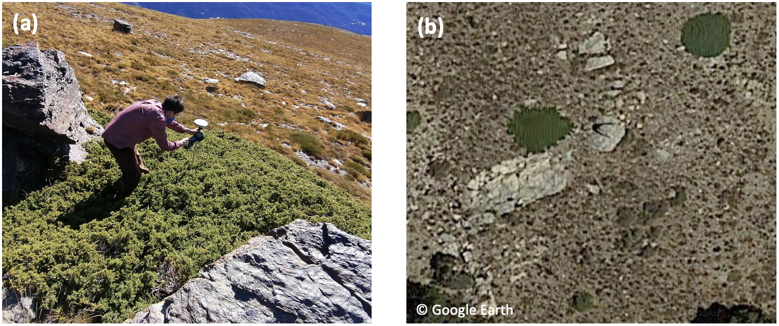
Figure 2: Visualization of Juniperus communis L. shrub located in the National Park of Sierra Nevada: (a) captured in-situ during the field work. (b) captured from Google Earth satellites.

Segmenting J. communis shrubs at high accuracy from satellite imagery with artificial intelligence remains more challenging than for common objects with fixed shapes such as those in bench-marking datasets like COCO (Common Objects in Context) (Lin et al. 2014). Junipers have complex growth patterns involving great variations in their sizes, colors, shapes, physiological status, distribution patterns, surroundings, and soil background (Fig. 3), which must be all considered.

2.3 Data acquisition

Since obtaining Field Work (FW) data is very expensive, labor-intensive, time-consuming, unsustainable, and limited to small spatial scale, we decided to create a Photo Interpreted (PI) data to have more flexibility in generating a large number of representative samples sufficient to train DL models. Therefore, two types of datasets were built in this study: a PI data used for model development, and a FW data used for model external validation. Both datasets contain pairs of input-output samples, collected from different sites in the National Park of Sierra Nevada, but they differ in the way these samples were collected and annotated (see subsections 2.3.1 and 2.3.2).

The input samples of both datasets contain RGB images, captured at $13cm$ spatial resolution, created as follows: first, RGB satellite images were downloaded from GE satellites at a maximum zoom of 21 using the coordinate reference system EPSG-4326 (WGS84), these scenes were cropped into small patches following a specific window size, then a selection process was applied in which we tried to cover the different land covers in Sierra Nevada as well as all Juniperus patterns described in Fig. 3. The output samples include shapefiles with Juniperus annotations corresponding to each input image.

In this study, a total of 836 images covering a set of 8580 shrubs were collected and annotated. A summarized description of both datasets in terms of Juniperus size is provided in Table 2 and Table 4, and the spatial distribution of these datasets is displayed in Fig. 4 and Fig. 5.

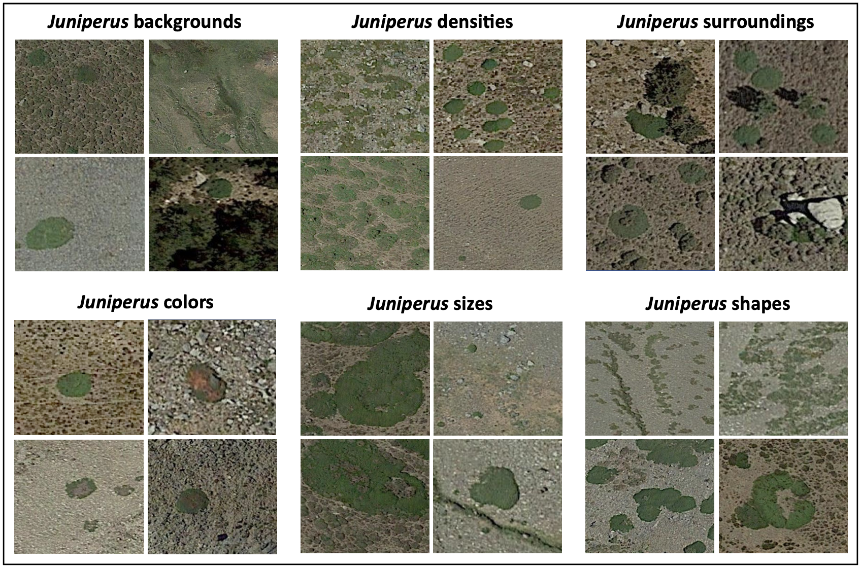
Figure 3: Samples of the different patterns of the studied Juniperus shrubs in the high mountains of Sierra Nevada captured by Google Earth satellites. These samples highlight the complex growth patterns of these shrubs.

2.3.1 Photo Interpreted (PI) dataset

The annotations of this dataset were manually created by experts using a visual inspection of the downloaded satellite images through a GIS (Geographic Information System) software (Fig. 4). This data is well distributed over all the National Park (Fig. 4). Only shrub images with high experts’ confidence were selected which implies that images with complicated patterns were excluded. This data contains a total number of 712 images of size (448 x 448), including a set of 6809 shrubs (Table 4), where each image covers an area of size $3392m^{2}$.

2.3.2 Field Work (FW) dataset

The annotations of this dataset were created by experts using an in-situ inspection of three different accessible field sites (Fig. 5). To do this, experts went to the field, delimited an area with a specific size ($2385m^{2}$), then took the geographic location of the center of each encountered Juniperus using a GPS (Global Positioning System) device. These locations were afterwards uploaded to a GIS software for a manual delineation of their corresponding shrubs. This data contains a total number of 124 images of size (420 x 336), including a set of 1771 shrubs (Table 4), where each image covers an area of size $2385m^{2}$.

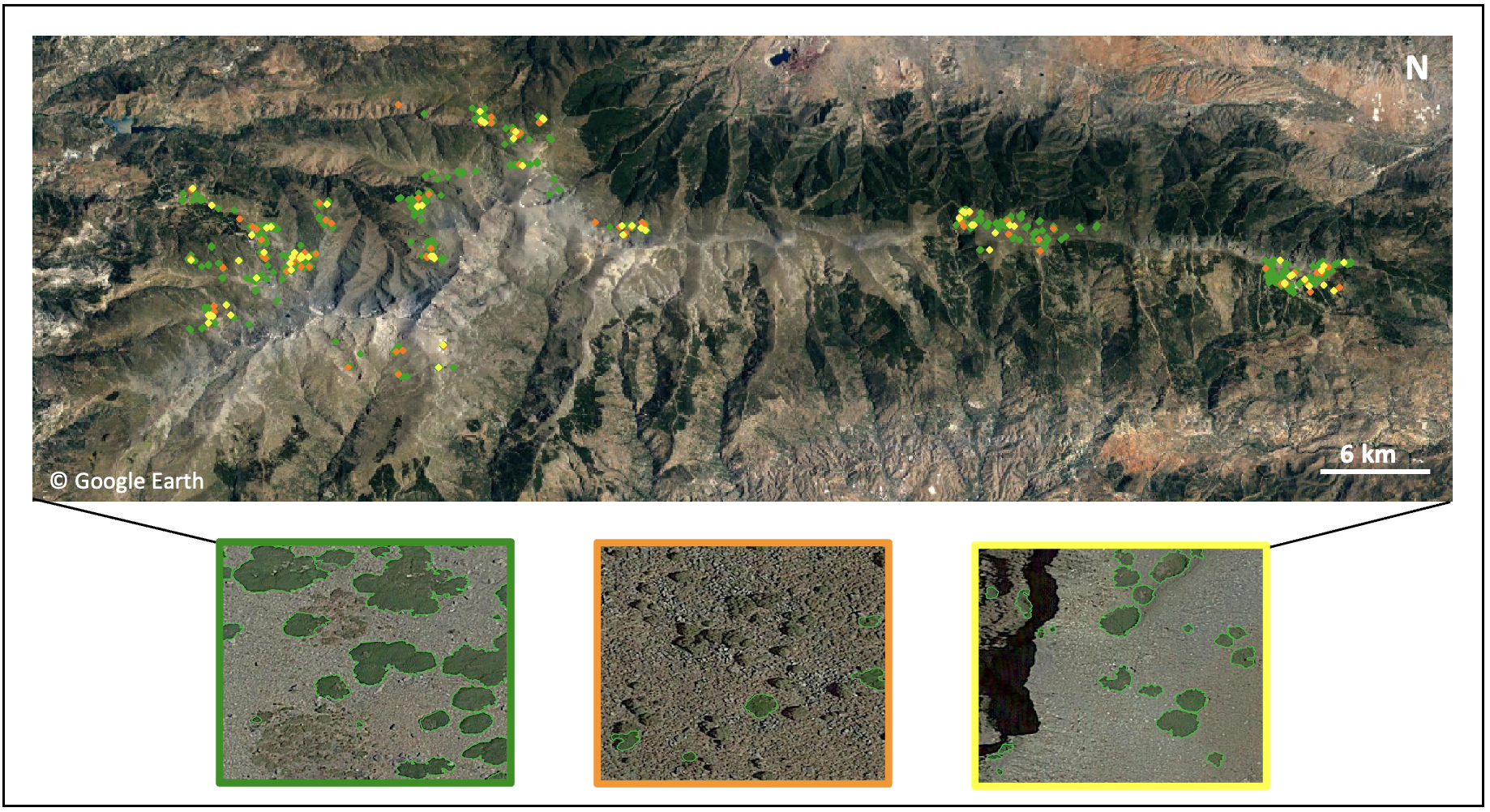
Figure 4: Distribution of the photo interpreted (PI) dataset in the National Park of Sierra Nevada (Andalusia, Spain). Three data partitions are highlighted: train data (green boxes), test data (orange boxes), and validation data (yellow boxes). The green segmentations delineate Juniperus shrubs.

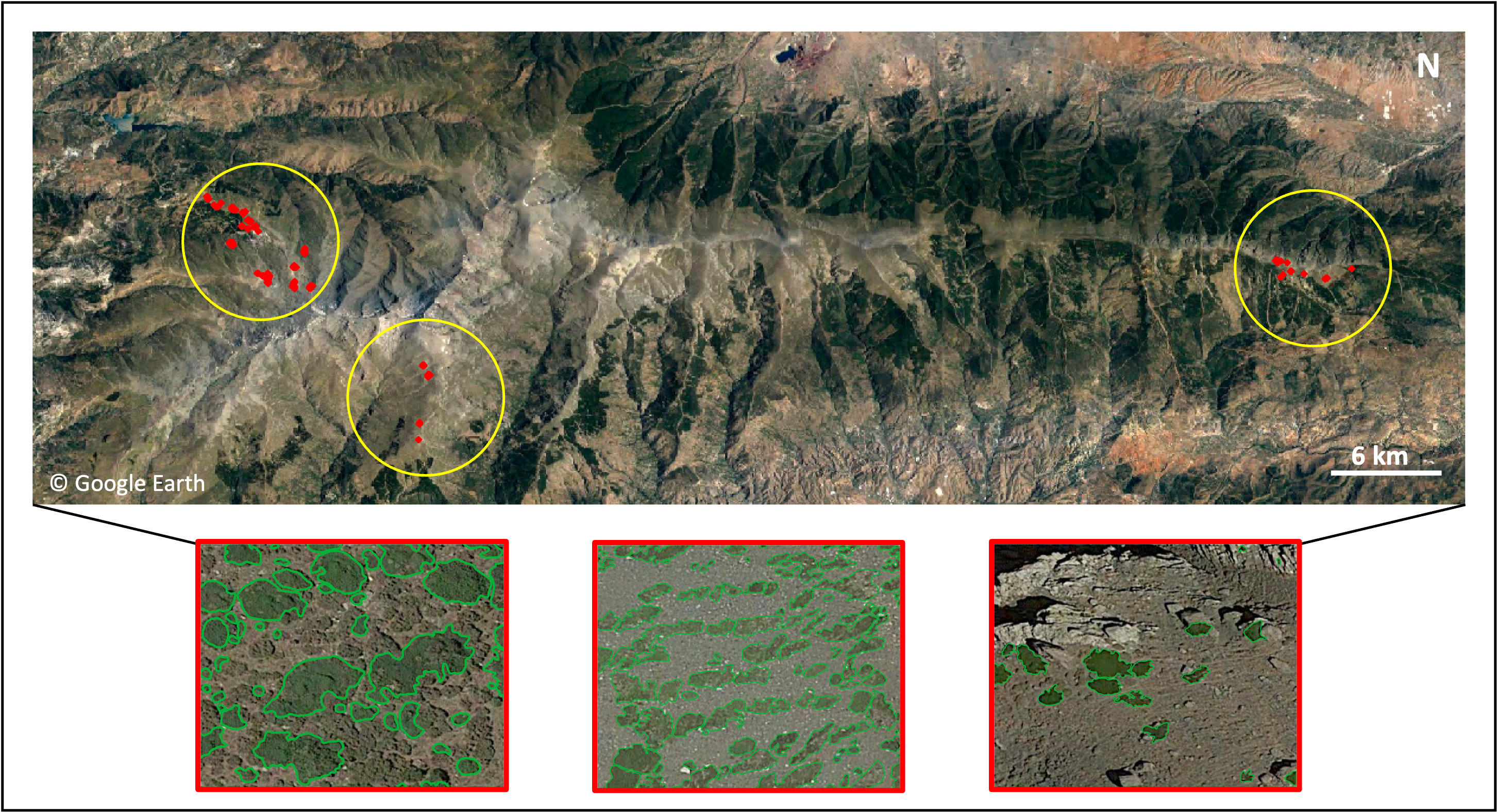
Figure 5: Distribution of the field work (FW) dataset collected from three different sites (yellow circles) in the National Park of Sierra Nevada (Andalusia, Spain). Red boxes display annotated samples from the field work data. The green segmentations delineate Juniperus shrubs.

Table 2: Statistical description of Juniperus size per square meters.

Data name	Statistics per size ($m^{2}$)
	Mean	Std	Min	25%	75%	Max	Count
Photo interpreted	19.97	42.39	0.13	3.62	20.82	761.42	6809
Field work	15.99	38.75	0.16	2.36	16.42	970.60	1771

Table 3: Description of shrub size classification schema. Six classes were defined corresponding to each quantile range: extra small (XS), small (S), medium (M), large (L), extra large (XL), and extra extra large (XXL).

	Shrub size categories
	XS	S	M	L	XL	XXL
Range (m2)	$[0.13,1.72[$	$[1.72,3.62[$	$[3.62,9.08[$	$[9.08,20.82[$	$[20.82,41.06[$	$[41.06,\infty[$
Quantiles (%)	$0-10$	$10-25$	$25-50$	$50-75$	$75-90$	$90-100$

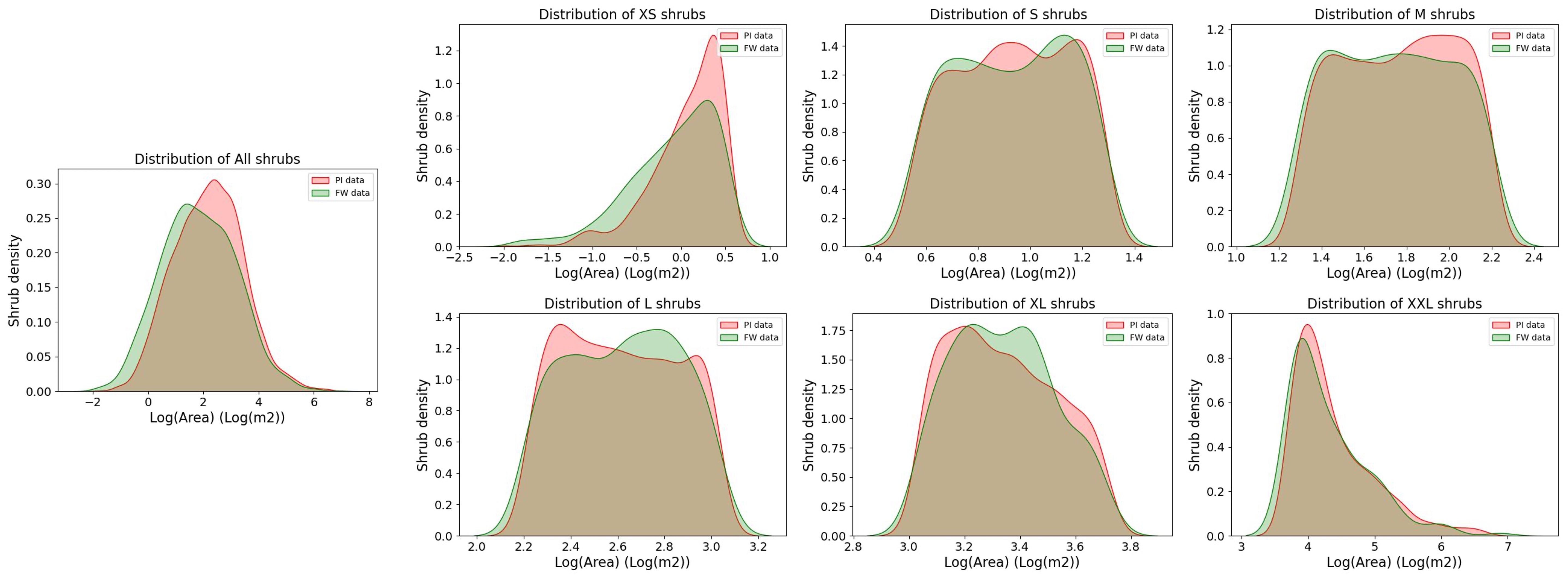
Figure 6: Logarithmic distribution of Juniperus areas in the photo interpreted (PI) and the field work (FW) datasets with respect to each size range: extra small (XS), small (S), medium (M), large (L), extra large (XL), and extra extra large (XXL).

Table 4: Distribution of the number of images and instances in photo interpreted and field work datasets over six size ranges: extra small (XS), small (S), medium (M), large (L), extra large (XL), and extra extra large (XXL).

Data name	Data partitions	Size of images	Number of images	Number of shrubs
				All	XS	S	M	L	XL	XXL
Photo Interpreted	Train	(448 x 448)	570	5459	559	837	1392	1331	805	535
	Test		75	690	29	91	163	201	119	87
	Validation		67	660	90	91	152	170	97	60
Field Work	External Validation	(420 x 336)	124	1771	310	329	439	351	194	148
Total			836	8580	988	1348	2146	2053	1215	830

2.3.3 Shrub size categorization

Notably, Juniperus exhibits a significant variation in its size (Table 2 and Fig. 6). In the PI dataset, the smallest shrubs measure $13cm^{2}$, while the largest ones span an impressive $761.42m^{2}$. Similarly, in the FW dataset, Juniperus shrubs range from $16cm^{2}$ to as large as $970.60m^{2}$. As a result, we categorized the shrubs into six distinct groups based on their size ranges (Table 3): extra small (XS), small (S), medium (M), large (L), extra large (XL), and extra extra large (XXL). This categorization was created using the PI data quantiles, since it is well distributed over all the park than the FW data. Fig. 6 displays the distribution of Juniperus area in both datasets PI and FW over the different size ranges. It can be noticed that these distributions are approximately similar, while the FW distribution is always wider than the PI distribution because it includes more complicated patterns than the PI data reflecting the real world observations.

3 Methods

This section describes the methodology used to develop the workflow of individual segmentation of Juniperus shrubs from RGB very-high resolution images collected from GE satellites at 13 cm spatial resolution.

3.1 Study design

The design of this study is organized into four main steps (Fig. 7): (1) the PI and the FW data were collected, annotated, and preprocessed, (2) the shrub delineation model was developed using the PI data, (3) the best model setup for deployment was determined using FW data, then (4) the model deployment was performed to generate a wall-to-wall map of Juniperus.

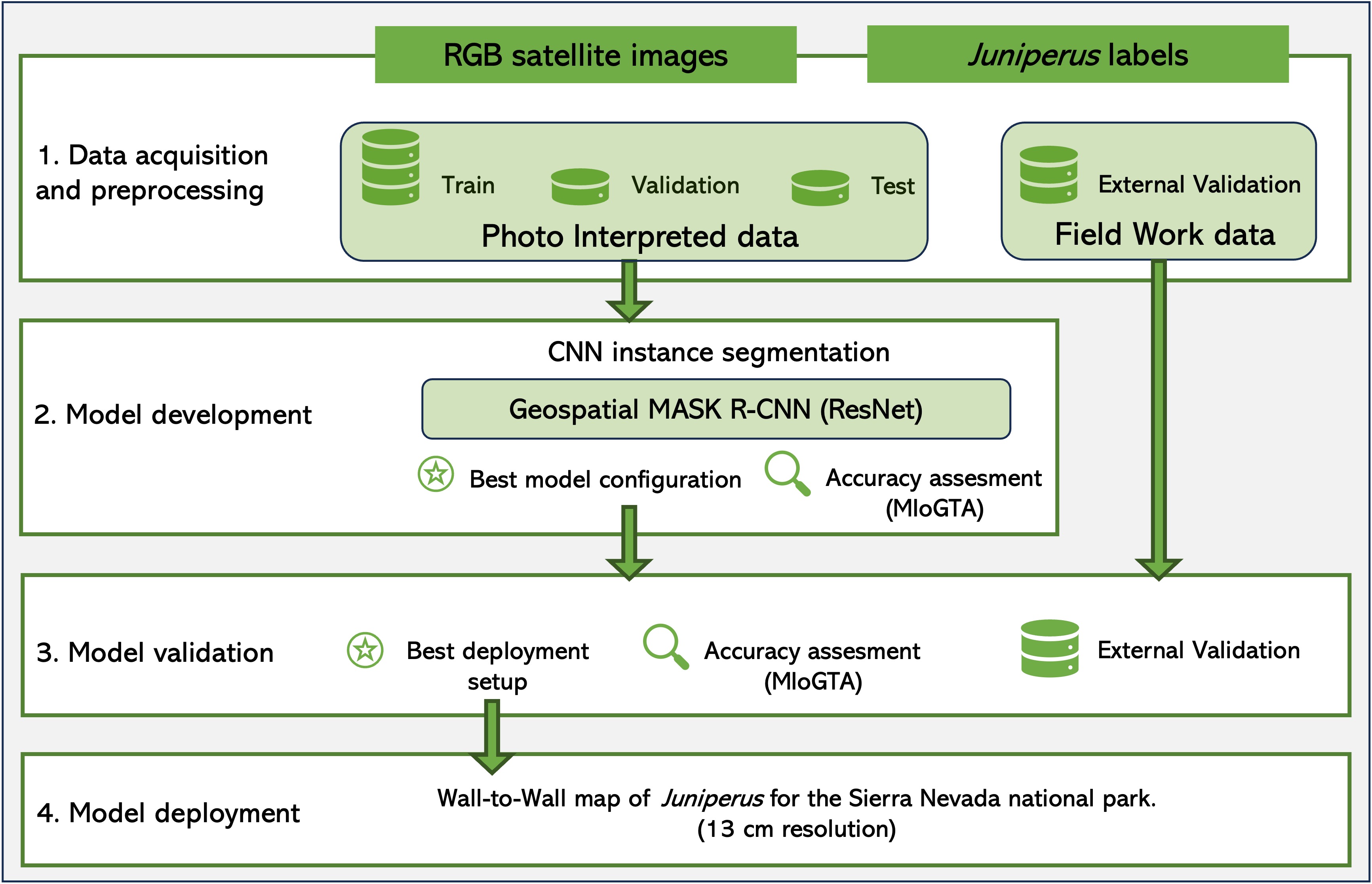
Figure 7: Workflow illustrating the process of automatic delineation of Juniperus shrubs.

3.2 Data preparation

The PI data was partitioned into three subsets: 1) train set which contains 80% of images to be used to train the model, 2) test set which contains about 10% of images to be used to evaluate the generalization capacity of the model on new examples from the PI data, and 3) validation set which contains about 10% of images to be used to regularize the model during the training process. The model regularization consists in evaluating the model performance on the validation data each 10 epochs during the training process, then save the best model state. The number of images and the number of shrubs for each data partition and for each shrub range size are stated in Table 4.

3.3 Model development

Deep learning models have shown impressive results in a variety of DL-based computer vision applications (Nguyen et al. 2024, Voulodimos et al. 2018, Chai et al. 2021, Khaldi & Shah 2021). Instance segmentation is a DL task that integrates both object detection with semantic segmentation. Mask R-CNN is a powerful DL model architecture that was used in various computer vision applications to perform the task of instance segmentation, particularly in individual vegetation delineation (Sani-Mohammed et al. 2022, Sun et al. 2022, Gené-Mola et al. 2020, Tian et al. 2020, Champ et al. 2020, Zheng et al. 2022, Kierdorf et al. 2023).

In this context, we adapted the model architecture Mask R-CNN (He et al. 2017), developed by META AI, to handle geospatial input/output data and perform a delineation of individual Juniperus shrubs. This architecture is the best release of instance segmentation when tested on Microsoft COCO benchmark. It is developed within computer vision library called Detectron2. This library contains a zoo of models with different backbone architectures already trained on COCO dataset (Lin et al. 2014). We adapted and re-trained all the available architectures of instance segmentation models to solve our task. This process, known as transfer learning, enables the reduction of both training time and the volume of data required to achieve good model performance (Weiss et al. 2016).

The Mask R-CNN architecture adapted to handle geospatial data is presented in Fig 8. This model contains the following five blocks (Fig 8 (a)):

1. The backbone network is a CNN model that extract feature maps from the input image.

2. The Region Proposal network (RPN) is responsible for scanning the feature maps generated by the backbone, then proposing regions, called Region of Interests (RoIs), that may potentially contain objects. The number of RoIs proposed by this network is always reduced using the Non-Maximum Suppression (NMS) operation.

3. The RoIAlign is used to extract a fixed-size feature map corresponding to each RoI proposed by RPN using the original feature maps generated by the backbone.

4. The Box head is a Fully Connected (FC) layer that flattens the feature maps provided by the RoIAlign into feature vectors, then maps these laters to the final $n$ number of classes and to the $4n$ bounding box coordinates. It includes two sub-heads, a classification head that classifies each RoI into object classes or background, and a regression head that refines the bounding box coordinates of each RoI.

5. The Mask head is responsible for generating a pixel-wise mask for each fixed-size feature map generated by the RoIAlign block. It consists of convolutional layers followed by deconvolutional (transpose convolution) layers to generate a mask with the same size as the original image. The generated masks are binary where each pixel is classified as either belonging to the object or the background.

The model generates for each detected shrub three kinds of outputs: 1) the bounding box coordinates of the region where the detected shrub is located, 2) a confidence score indicating the model’s level of certainty that the identified shrub is indeed a Juniperus, and 3) a mask highlighting all the pixels belonging to the detected shrub. After output generation, a postprocessing pipeline is performed to filter, refine and georeference the results. This includes four main steps: (1) the NMS process to eliminate redundant bounding boxes (using a threshold of $50\%$), (2) thresholding to refine mask predictions by removing detections with low confidence score, (3) georeferencing to associate each binary mask with the geographic coordinates of the input image, and (4) polygonizing to convert the georeferenced binary mask into a shape file of polygon(s) delineating each shrub while saving its corresponding confidence score (Fig 8 (b)).

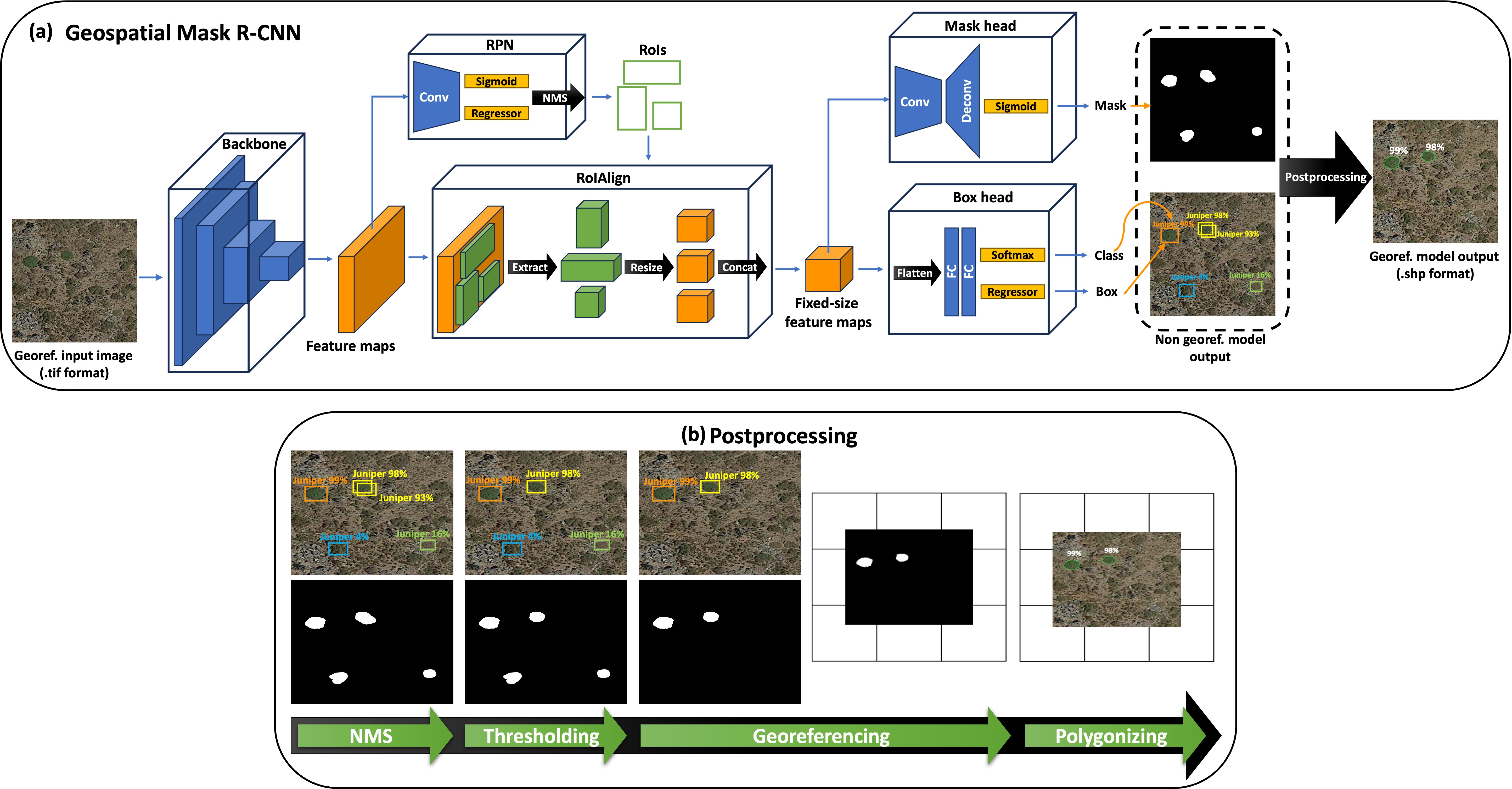
Figure 8: Description of the model design used to delineate Juniperus shrubs. (a) Description of the geospatial Mask R-CNN architecture used in this study. (b) Description of the postprocessing pipeline used to generate the final georeferenced output.

To find the best Mask R-CNN model in our case, a hyperparameter optimization process was applied on different combinations of hyperparameters: maximum number of iterations, optimization algorithms, learning rate values and schedulers, maximum number of boxes per image to sample from the RPN, type of transformations to use within data augmentation, and backbone architectures (Carvalho et al. 2020).

3.4 Model evaluation

In computer vision, an ordinary object may have different sizes and colors but maintains the same spatial signature characterizing its identity. Juniperus shrubs, on the contrary, are one of the living organisms exhibiting a complex growth patterns (i.e., high variations in their spatial distribution): (1) they can grow not only in different sizes and colors but also in different shapes and densities (Fig. 3). (2) They can follow aggregated growth patterns where individual shrubs share a close proximity and can overlap or grow in clusters. (3) They can follow a ramifying growth patterns where individual shrubs divide into distinct parts. This complex character can mainly depend on the geographic, topographic, and climatic conditions.

All these factors make the identification of Juniperus by experts through satellite images confusing, and their annotation process challenging. One expert may identify a shrub as one individual while others may see it as multiple individuals (i.e., a cluster/colony of shrubs). This subjectivity introduces uncertainty in the annotation process and makes the model prone to generate one detection enclosing a set of annotated shrubs and/or multiple partial detections for one annotated shrub. An example of this model behavior is depicted in Fig. 9, where the yellow delineations refer to the model detections and the green ones to the expert annotations.

Given the aggregated/ramifying growth patterns of Juniperus, the partial detections made by the model for one annotated shrub or the single detection made for a colony of annotated shrubs are still correct from the ecological perspective. The main goal of ecologists in this case is to have a model able to localize the shrub position while delineating a great percentage of its area, regardless of how the model see the shrub (i.e., as one individual or colony of individuals).

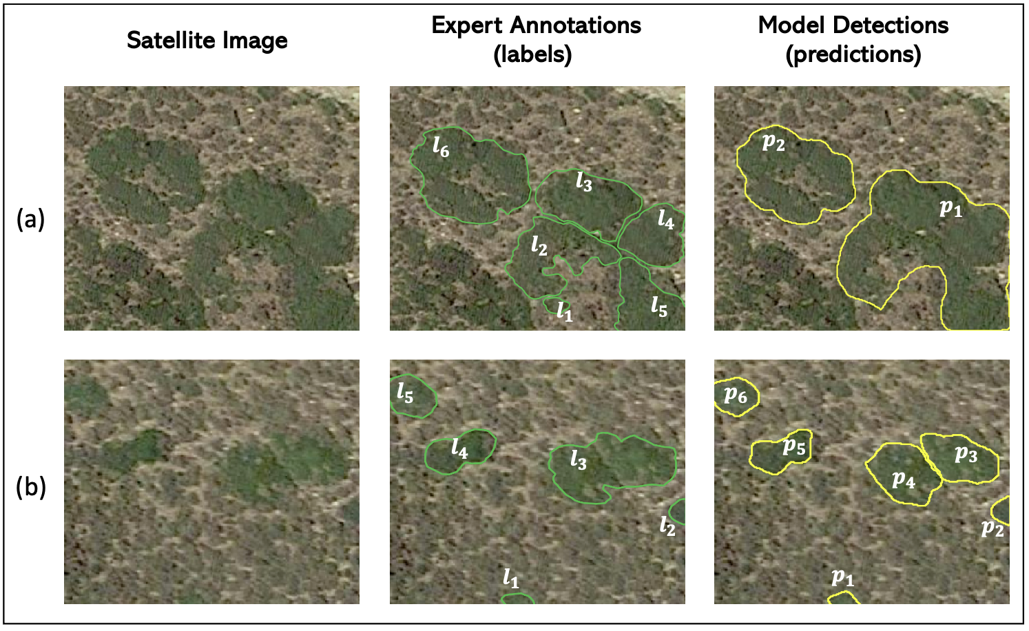
Figure 9: Two examples showing a high discrepancy between expert annotations $l$ (in green) and model detections $p$ (in yellow): (a) the expert annotated a cluster of shrubs ($l_{1}$ to $l_{5}$) but the model detected one individual shrub ($p_{1}$). (b) the expert annotated one individual shrub ($l_{3}$) but the model detected a cluster of two individual shrubs ($p_{3}$ and $p_{4}$).

The number of TPs (true positives), FPs, and FNs made by object detection and instance segmentation models are often evaluated using the Intersection over Union (IoU) metric. This metric computes the area of the intersection between the prediction $p$ and the label (i.e., ground truth) $l$ and divide the result by the area of their union (Eq. 1). It evaluates the matching amount between the prediction and the labels. Here, the prediction and the label could be the shrub’s bounding box or segmentation depending whether one is evaluating the object detection head or the mask head, respectively.

$$IoU(p,l)=\frac{Area(p\cap l)}{Area(p\cup l)}$$ (1)

The evaluation process includes two main steps: (1) predictions evaluation step where the algorithm iterates over the predicted instances to compute the number of TPs and FPs, and (2) labels evaluation step where the algorithm iterates over the ground truth instances to get the number of FNs. This evaluation process is described in details in Algorithm 1 in A.

To compute the number of TPs and FPs, the IoU-based evaluation algorithm iterates over each prediction $p_{i}\in S_{p}$, and looks for all overlapping ground truth $l_{j}\in S_{l}$, then picks the best matching ground truth $l_{match}$ with the highest value of IoU: $l_{match}=\arg\max_{l_{j}\in S_{l}}IoU(p_{i},l_{j})$. Similarly, to compute the number of FNs, this algorithm iterates in this case over each ground truth $l_{j}\in S_{l}$, and looks for all predictions $p_{i}\in S_{p}$ overlapping with this ground truth, then selects the best matching prediction $p_{match}$ with the highest value of IoU: $p_{match}=\arg\max_{p_{i}\in S_{p}}IoU(l_{j},p_{i})$.

If we use the IoU metric to evaluate the model in the case of plants with aggregated/ramifying growth patterns, we will end up with many false detections (FPs) and overlooked detections (FNs). This is mainly because IoU is totally dependent on the quality of annotations since it considers them as a reference to evaluate the accuracy of the model predictions. Figure 9 shows two examples in which although the model detects all the existing shrubs, this metric penalizes the model for being not aligned with the existing annotations made by the expert. In example (a) of Figure 9, the expert annotated six shrubs $\{l_{j}:j\in[1:6]\}$ but the model generated only two predictions $\{p_{1},p_{2}\}$, such that the detection $p_{1}$ includes all the five annotated shrubs. During the evaluation process, the algorithm will classify the labels $\{l_{j}:j\in[1:5]\}$ as FNs and the corresponding prediction $p_{1}$ as FP. Alternatively, in example (b) of Figure 9, the expert annotated five shrubs $\{l_{j}:j\in[1:5]\}$ but the model generated six predictions $\{p_{i}:i\in[1:6]\}$, such that the label $l_{3}$ is covered by two detections $p_{3}$ and $p_{4}$. Again, during the evaluation process, the label $l_{3}$ will be classified as FN.

Accordingly, we can consider in this case that the IoU-based evaluation process is biased to the uncertainty in the data annotation, then turns to be unfair and not reflective to the real model performance, and does not comply with the main goal of this application. Therefore, creating a new metric less sensitive to data annotation uncertainty (i.e., independent of how shrubs have been annotated by experts) is necessary to evaluate the model performance in identifying this kind of plants with complex growth patterns.

In this regard, we propose a shrub-tailored evaluation process using a new evaluation metric called Multiple Intersections over Ground Truth Area (MIoGTA). Unlike the IoU that evaluates the predictions and labels similarly, this metric has two formulas, one to evaluate the predictions to get the number of TPs and FPs (Eq. 2), and another one to evaluate the labels to get the number of FNs (Eq. 3). The main concept behind this metric is to count all matching shrubs in the evaluation of labels and predictions (Fig 10 (b),(d)), rather than focusing solely on the best-matching shrub as performed by IoU metric (Fig 10 (a),(c)).

To evaluate a prediction $p$, we look for the set of all matching labels $S_{l_{match}}$. Subsequently, we calculate the area of the intersection between $p$ and $S_{l_{match}}$, we then divide this area by the area of all matching labels $S_{l_{match}}$ to evaluate how much of the labels’ areas are covered by the prediction $p$. The predictions evaluation process is defined in Eq. 2 by the metric $MIoGTA(p,S_{l_{match}})$ and visualized in Fig 10 (b).

$$MIoGTA(p,S_{l_{match}})=\frac{Area(p\cap\bigcup_{k=1}^{|S_{l_{match}}|}l_{k})}{Area(\bigcup_{k=1}^{|S_{l_{match}}|}l_{k})}$$ (2)

To evaluate a label $l$, we look for the set of all matching predictions $S_{p_{match}}$. Afterwards, we calculate the area of the intersection between $l$ and $S_{p_{match}}$, we then divide this area by the area of the label $l$ to evaluate how much of the label’s area is covered by the set of predictions. In this case, the score that is going to be attributed to the label $l$ will be the maximum score over the $p_{k}$ predictions where $k\in\{1,...,|S_{p_{match}}|\}$. The labels evaluation process is defined in Eq. 3 by the metric $MIoGTA(l,S_{p_{match}})$ and visualized in Fig 10 (d).

$$MIoGTA(l,S_{p_{match}})=\frac{Area(l\cap\bigcup_{k=1}^{|S_{p_{match}}|}p_{k})}{Area(l)}$$ (3)

In Eq. 2, $p$ denotes the prediction made by the model, $S_{l_{match}}$ is the set of all matching labels made by experts, and $l_{k}$ is the matching label $k$. In Eq. 3, $l$ denotes the label made by experts, $S_{p_{match}}$ is the set of all matching predictions made by the model, and $p_{k}$ is the matching prediction $k$. Both the labels and predictions can refer to either bounding boxes or segmentations. The whole evaluation protocol, including predictions and labels evaluation, is explained in Algorithm 2 in A.

Using the number of TPs, FPs, and FNs generated by Algorithm 2, three evaluation metrics can be computed to evaluate the model performance for shrubs delineation: (1) the $Precision$ (4) to assess how precise the model is in delineating the shrubs, (2) the $Recall$ (5) to evaluate how accurate the model is in recalling the shrubs, and (3) the $F1-score$ (6) to examine the ability of the model to maintain the trade-off between the Precision and the Recall.

$$Precision=\frac{TP}{TP+FP}$$ (4)

$$Recall=\frac{TP}{TP+FN}$$ (5)

$$F1-score=\frac{2*Precision*Recall}{Precision+Recall}$$ (6)

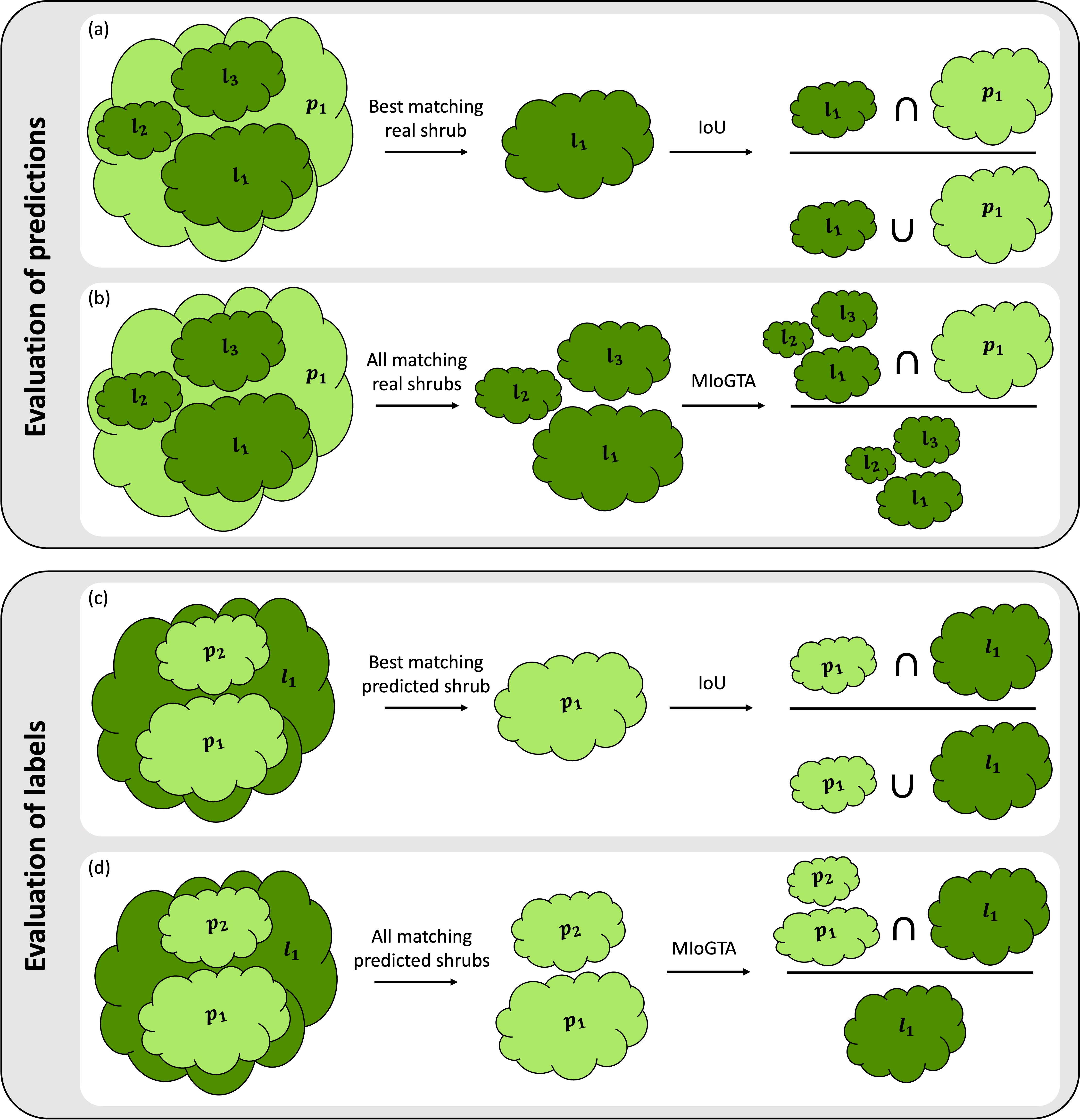
Figure 10: Graphics showing the difference between IoU and MIoGTA metrics for predictions and labels evaluation. Figures (a) and (b) present an example where the expert annotated a cluster of shrubs but the model detected one shrub, then explain how the model prediction is evaluated using the IoU and MIoGTA, respectively. Figures (c) and (d) present an example where the expert annotated one shrub but the model detected a cluster of shrubs, then explain how the expert label is evaluated using the IoU and MIoGTA, respectively. $p$ denotes the model predictions (light green) and $l$ the expert annotations (dark green).

3.5 Model deployment

After developing the model using the PI data and validating the model using the FW data, it was deployed over all the park of Sierra Nevada to generate a wall-to-wall map of all Juniperus shrubs. The deployment pipeline consists in seven main steps (Fig. 11): (1) A set of RGB tiles covering the whole park were downloaded at 13 cm resolution. (2) Each tile was cropped into images of size (448 x 448). (3) A DEM (Digital Elevation Model) at 2m/pixel resolution was used to filter out images with altitude less than 1.9km because we assume that Juniperus is more likely to grow above this altitude and the model is more prone to make false detections below this altitude. To perform this filtering, each image was assigned an altitude value corresponding to the maximum altitude covered by the image. (4) The filtered images were, afterwards, conveyed to the model in order to individually delineate the shrubs. (5) Even after applying the NMS operation, the model can still generate multiple detections of the same shrub. For this reason, a refining process was applied to these detections that consists in dissolving the multiple detections of the same shrub in one detection using the union over their geometries and creating three kinds of scores (average, median, and maximum scores). (6) A second area-based filtering was applied, where we filtered out all the detections with area less than 1.04m2 because we are less confident in the model detections below this threshold. (7) All the detections of the images were merged to generate a final map of Juniperus for all the park at 13cm resolution.

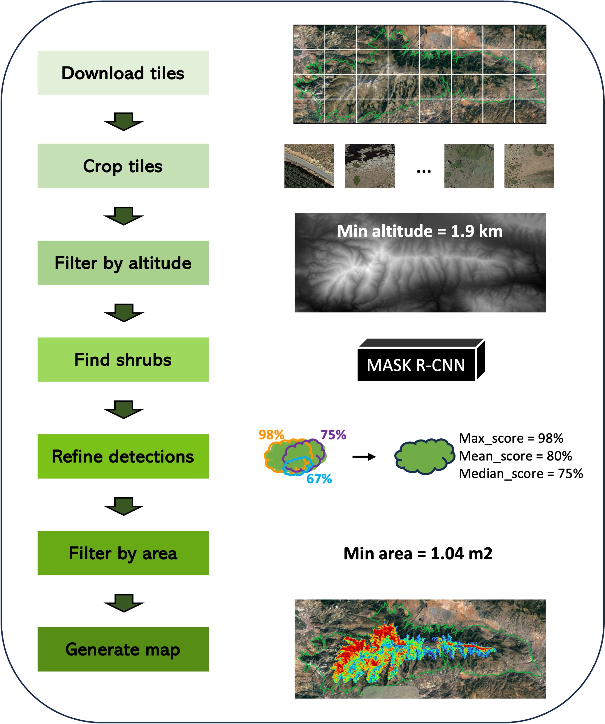
Figure 11: Description of the deployment pipeline.

4 Results

4.1 Finding the best model configuration

The best model configuration was obtained after training the model with 4000 iterations using Momentum optimization algorithm with a mini-batch size of two images. This algorithm was optimized using an adaptive learning rate called WarmupCosine scheduler where a warm-up phase with a low learning rate of value 0.0025 started, then the learning rate was gradually decreased by 10 in a cosine-like manner after each 2000 epochs. In our study, data augmentation was not used because it showed no significant improvement in the model performance and this is because our data size is very large. In addition, the hyperparameter optimization process showed that 256 is the best maximum number of RoIs to sample from the RPN network, while, the backbone architecture ResNet101-C4 is the best feature extractor for Mask R-CNN in both shrub detection and delineation. Table 5 presents the results of all the used backbones, where AP, AR, and AF1 refer to average precision, average recall, and average F1-score over MIoGTA metric thresholds ranging from 50% to 95% with a step of 5% $(\theta_{MIoGTA}\in[50:5:95]\%)$, respectively. The best model configuration using the evaluation metric $MIoGTA$ is described in Table 6.

Table 5: Comparison between the different Mask R-CNN backbones using the test data at confidence score threshold $\theta_{score}=90\%$. AP, AR, and AF1 refer to average precision, average recall, and average F1-score over MIoGTA metric thresholds $(\theta_{MIoGTA}\in[50:5:95]\%)$.

Backbones	Box			Mask
	AP	AR	AF1	AP	AR	AF1
ResNet50-C4	56.33	65.28	60.46	73.75	72.78	73.26
ResNet50-DC5	54.15	67.12	59.92	73.15	76.39	74.73
ResNet50-FPN	60.65	64.89	62.68	78.82	72.89	75.74
ResNet101-C4	59.55	69.47	64.11	78.27	77.26	77.76
ResNet101-DC5	56.09	63.62	59.60	75.14	72.98	74.04
ResNet101-FPN	63.63	55.06	59.02	80.99	62.14	70.32
ResNeXt101-FPN	65.93	57.16	61.23	81.68	63.93	71.72

Table 6: Description of the best Mask R-CNN configuration used in the automatic delineation of individual shrubs.

Hyperparameters	Best values
Maximum number of iterations	4000
Optimization algorithms	Momentum
Batch size	2
Learning rate	0.0025
Learning rate scheduler	WarmupCosine
Data augmentation	No augmentation
Maximum number of boxes	256
Feature extractor (backbone)	ResNet101-C4

4.2 Comparing between the proposed evaluation metric MIoGTA and IoU metric

After choosing the optimal Mask R-CNN architecture, we assessed the performance of the proposed MIoGTA metric in comparison to the standard IoU metric at a confidence score threshold $\theta_{score}=90\%$ using the test dataset. Tables 7 and 8 present the model’s performance for both shrub detection and delineation, respectively. These results are presented for two different metric thresholds: 50% and 75%.

For shrub detection, the use of the MIoGTA metric resulted in a significant reduction in the number of FNs, while the FPs showed an opposing trend (Table 7). In addition, the IoU metric demonstrates superior performance compared to MIoGTA at thresholds 50% and 75%, achieving F1-scores of 84.82% and 72.46% as opposed to 80.62% and 70.00%, respectively. On the other hand, for shrub delineation, both FPs and FNs decreased significantly which make MIoGTA outperform the IoU metric across all thresholds 50% and 75% achieving F1-scores of 87.87% and 84.77%, respectively, surpassing F1-scores of IoU: 84.84% and 73.95%, respectively (Table 8).

Unlike IoU metric, MIoGTA results showed that there is a high discrepancy between the model performance in shrubs detection (80.62%) and shrub delineation (87.87%). This discrepancy can be attributed to the fundamental concept of considering all matching predictions and labels when evaluating the label-to-prediction relationship. In cases where a cluster of shrubs is present, even if their shapes do not overlap, their bounding boxes often intersect. Thus, during the detection evaluation, many FPs are generated (Table 8), which explains the large gap between model performance in shrub delineation and shrub detection.

Thereafter, we can conclude that the proposed metric is very powerful to evaluate the model ability to solve instance segmentation tasks but not object detection tasks. Since the main objective of our study is to create a model able to delineate shrubs with high accuracy, the proposed MIoGTA was selected as the best evaluation metric to determine the number of TPs, FPs, and FNs.

Table 7: Comparison between MIoGTA and IoU metrics in evaluating the Mask R-CNN ability for shrub detection using the test data at confidence score threshold $\theta_{score}=90\%$.

metric name	metric threshold	TP	FP	FN	Precision	Recall	F1-score
IoU	50%	567	79	124	87.77	82.06	84.82
	75%	484	162	206	74.92	70.15	72.46
MIoGTA	50%	493	153	84	76.32	85.44	80.62
	75%	413	233	121	63.93	77.34	70.00

Table 8: Comparison between MIoGTA and IoU metrics in evaluating the Mask R-CNN ability for shrub delineation using the test data at confidence score threshold $\theta_{score}=90\%$.

metric name	metric threshold	TP	FP	FN	Precision	Recall	F1-score
IoU	50%	568	78	125	87.93	81.96	84.84
	75%	494	152	196	76.47	71.59	73.95
MIoGTA	50%	572	74	84	88.55	87.20	87.87
	75%	551	95	103	85.29	84.25	84.77

Figure 12 compared the metrics MIoGTA and IoU over different model confidence score thresholds $\theta_{score}$ for both tasks, shrub detection and delineation. For shrub detection, the IoU curve is slightly higher than the MIoGTA curve (Figure 12(a)). For shrub delineation, we notice an opposite behavior such that the gap between both curves is slightly low with threshold 50% but becomes widely high with threshold 75% (Figure 12(b)). Thus, we can confirm that MIoGTA is powerful in revealing the true ability of the model to delineate shrubs compared to IoU metric.

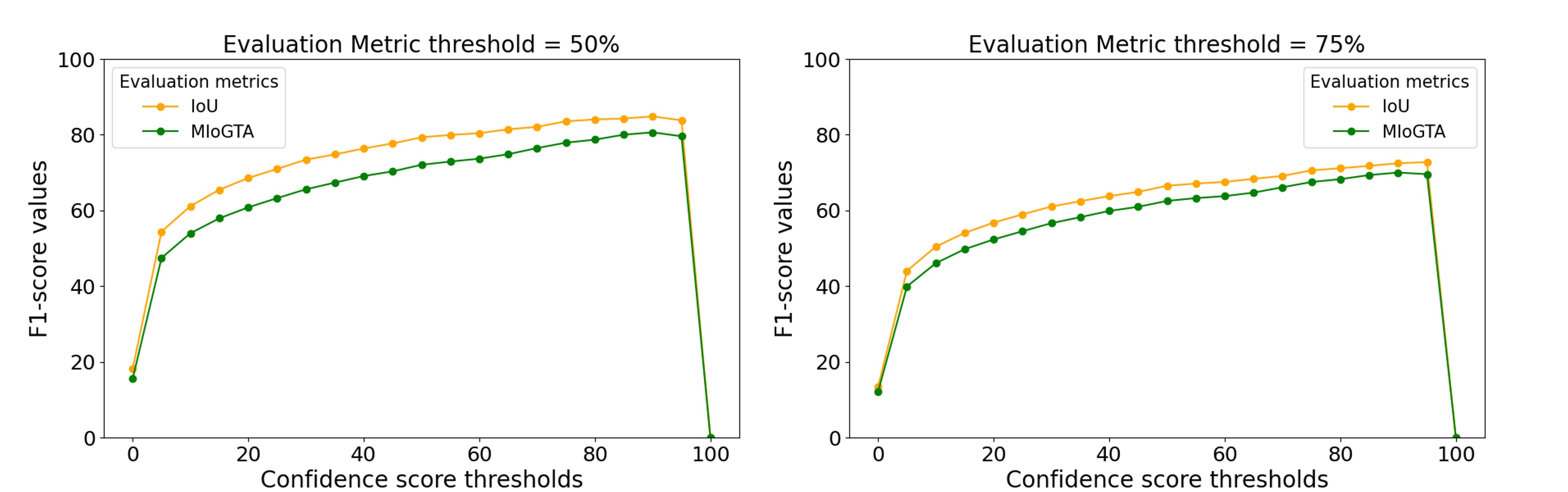
(a) Shrub detection evaluation.

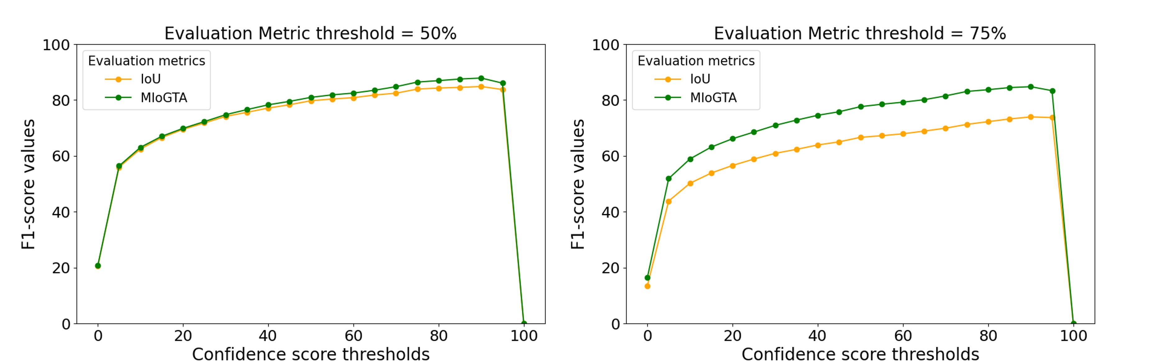
(b) Shrub delineation evaluation.

Figure 12: Representation of the Mask R-CNN performance after being evaluated by IoU and MIoGTA metrics, independently for the tasks of: (a) shrub detection and (b) shrub delineation. These figures display the F1-score curve for the test data over different confidence score thresholds $\theta_{score}$ ranging from 0% to 100%.

4.3 Finding the model deployment setup using the external validation data

To validate the model ability in delineating Juniperus shrubs, the external validation data belonging to the FW dataset was used. Figure 13 presents the F1-score values of the model applied on both test and external validation data over different confidence score thresholds $\theta_{score}$ ranging from 0% to 100%. Accordingly, we can notice that the two curves exhibit different patterns. The F1-score curve of the test data is monotonically increasing reaching a maximum confidence score at $\theta_{score}=90\%$. While the F1-score of the external validation data increases, then maintains a stationary behavior between confidence score 20% and 85% while hitting the maximum at $\theta_{score}=50\%$. Consequently, unlike PI data, the model performance in the FW data is approximately stable for any model confidence score threshold. Therefore, since the FW data is a snapshot of the real world data, the best confidence score threshold to use in the deployment process is $\theta_{score}=50\%$.

Table 9 highlights in detail the difference in model performance on the test and external validation data using the aforementioned best confidence score threshold $\theta_{score}$ in each case. Given that PI and FW datasets are sampled from totally different distributions, there is a drop of only 11.01% in the F1-score between both datasets at $\theta_{MIoGTA}=50\%$: $87.87\%$ in PI data and $76.86\%$ in FW data. This discrepancy is mainly due to the complicated patterns of the shrubs used in the FW data as well as to their data size: 1771 shrubs in the external validation data and 690 shrubs in the test data. Accordingly, we can still assert the efficiency of the dual data construction approach (i.e., developing the model using PI data and externally validating it using FW data) overcoming the challenging aspect of collecting samples from field surveying. Fig. 14 presents some samples of the model detections and their corresponding expert annotations for both PI (test data) and FW (external validation data) datasets.

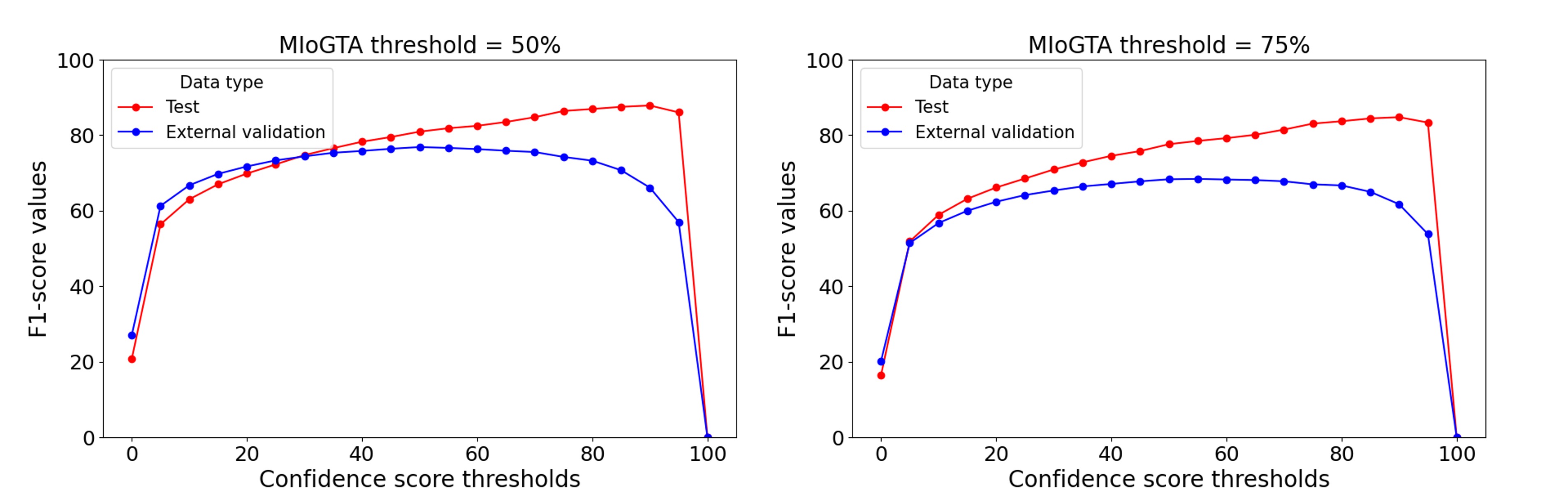
Figure 13: Representation of F1-score curves for both test data (red line) and external validation data (blue line) over different confidence score thresholds $\theta_{score}$, and at metric thresholds $\theta_{MIoGTA}$: $50\%$ and $75\%$.

Table 9: Comparison between Mask R-CNN performances for shrub delineation on test data at $\theta_{score}=90\%$ and external validation data at $\theta_{score}=50\%$.

Data name	MIoGTA threshold	TP	FP	FN	Precision	Recall	F1-score
PI data (Test)	50%	572	74	84	88.55	87.20	87.87
	75%	551	95	103	85.29	84.25	84.77
FW data (External Validation)	50%	1307	399	388	76.61	77.11	76.86
	75%	1141	565	493	66.88	69.83	68.32

4.4 Assessing the impact of Juniperus size on the model performance

To further explore the difference in the model performance between PI dataset (test) and FW dataset (external validation), we decided to evaluate the model with respect to the six different shrub size ranges (XS, S, M, L, XL, and XXL) (Table 10). The XL followed by L then XXL shrubs are very well delineated by the model with an F1-score above 92% for PI data and 83% for FW data. In addition, the M and S shrubs are well delineated with an F1-score above 78% and 73%, for the PI and FW dataset, respectively. However, the model finds more difficulty to delineate XS shrubs for both datasets: F1-score of 53.06% in PI dataset and 61.45% in FW dataset. All in all, either in the PI dataset (F1-score=87.87%) or in the FW dataset (F1-score=76.86%), the model performance is very promising given the difficulty of the shrub delineation task from RGB satellite images, the input complexity, and the label uncertainty.

Table 10: Comparison between model performances for shrub delineation on test data at $\theta_{score}=90\%$ and external validation data at $\theta_{score}=50\%$ over six size ranges: extra small (XS), small (S), medium (M), large (L), extra large (XL), and extra extra large (XXL) using $\theta_{MIoGTA}=50\%$.

Data name	Size	TP	FP	FN	Precision	Recall	F1-score
PI data (Test)	XS	13	11	12	54.17	52.00	53.06
	S	64	16	19	80.00	77.11	78.53
	M	128	23	28	84.77	82.05	83.39
	L	171	10	13	94.48	92.94	93.70
	XL	112	7	6	94.12	94.92	94.52
	XXL	84	7	6	92.31	93.33	92.82
	All	572	74	84	88.55	87.20	87.87
FW data (External Validation)	XS	165	96	111	63.22	59.78	61.45
	S	243	89	85	73.19	74.09	73.64
	M	319	129	86	71.21	78.77	74.80
	L	298	55	45	84.42	86.88	85.63
	XL	172	20	24	89.58	87.76	88.66
	XXL	110	8	37	93.22	74.83	83.02
	All	1307	399	388	76.61	77.11	76.86

4.5 Assessing the correlation between the real and the predicted shrub areas

To analyze the model performance from the shrub area perspective within the PI and FW data, a correlation analysis was performed between the area of the real shrubs that were detected by the model and the area of the model predictions. Fig. 15 displays the results of the correlation analysis for PI data (test) and FW data (external validation) with respect to all shrub sizes (XS, S, M, L, XL, and XXL). Accordingly, there is a high correlation between the areas of the real and predicted shrubs in both datasets: $r=0.99$ in PI data and $r=0.96$ in FW data for all sizes.

In the PI dataset, we observe strong correlations among shrub sizes. The XXL, XL, and M shrubs exhibit the highest correlations with coefficients of 0.99, 0.93, and 0.92, respectively. Meanwhile, the L and S shrubs display a remarkable correlations with coefficients of 0.88 and 0.87, respectively. The XS shrubs, though, exhibit the lowest correlation ($r=0.77$).

Similarly, within the FW dataset, we notice noteworthy correlations. The XXL and M-sized shrubs show significant correlations, with coefficients of 0.93 and 0.80, respectively. On the other hand, the L and XS shrubs demonstrate notable correlations of 0.73 and 0.72, respectively. In contrast, the XL and S shrubs have relatively weaker correlations, with values of 0.67 and 0.65, respectively.

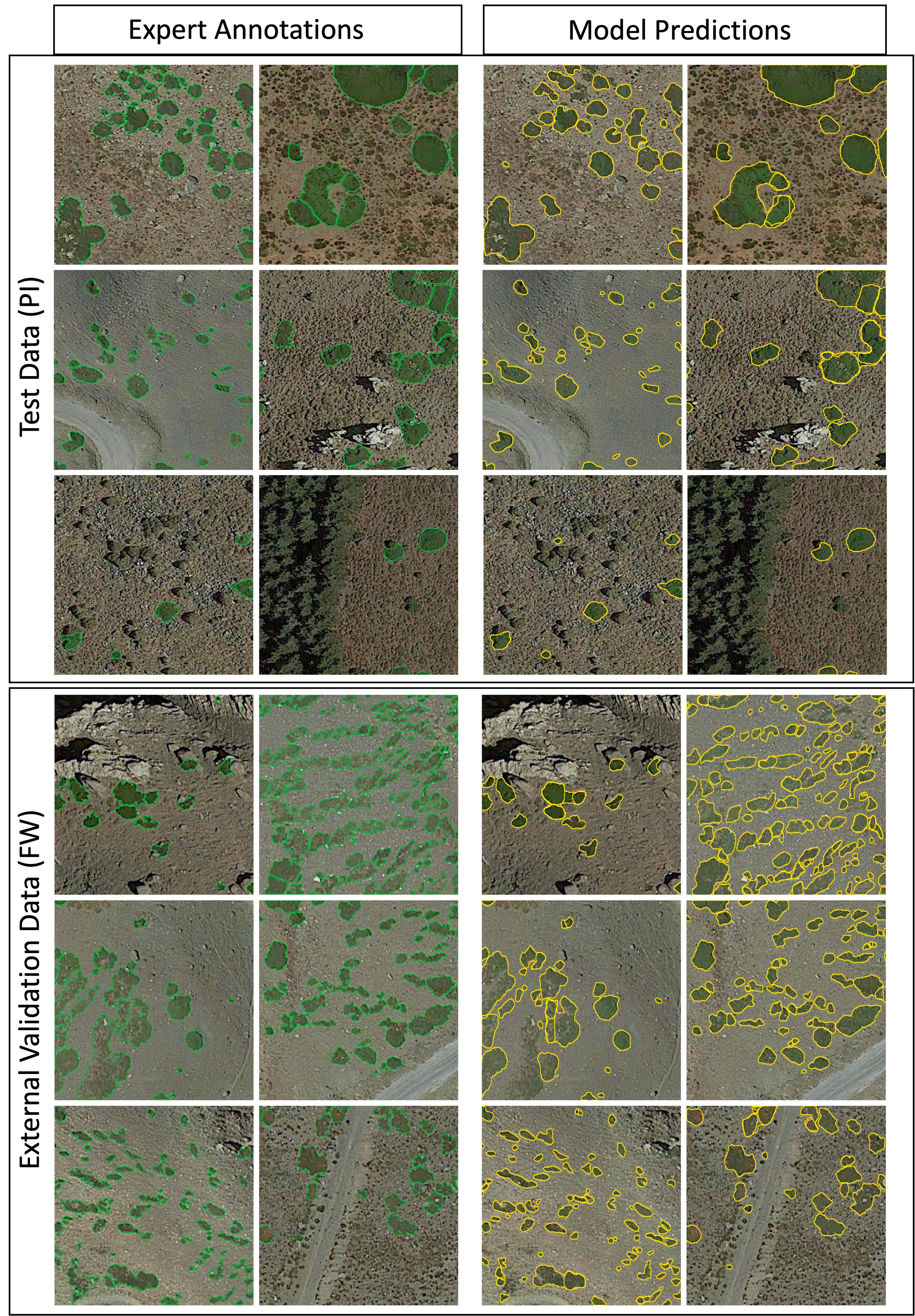
Figure 14: Samples of model predictions (in yellow) and their corresponding experts annotations (in green) from photo interpreted (PI) data at $\theta_{score}=90\%$ and field work (FW) data at $\theta_{score}=50\%$.

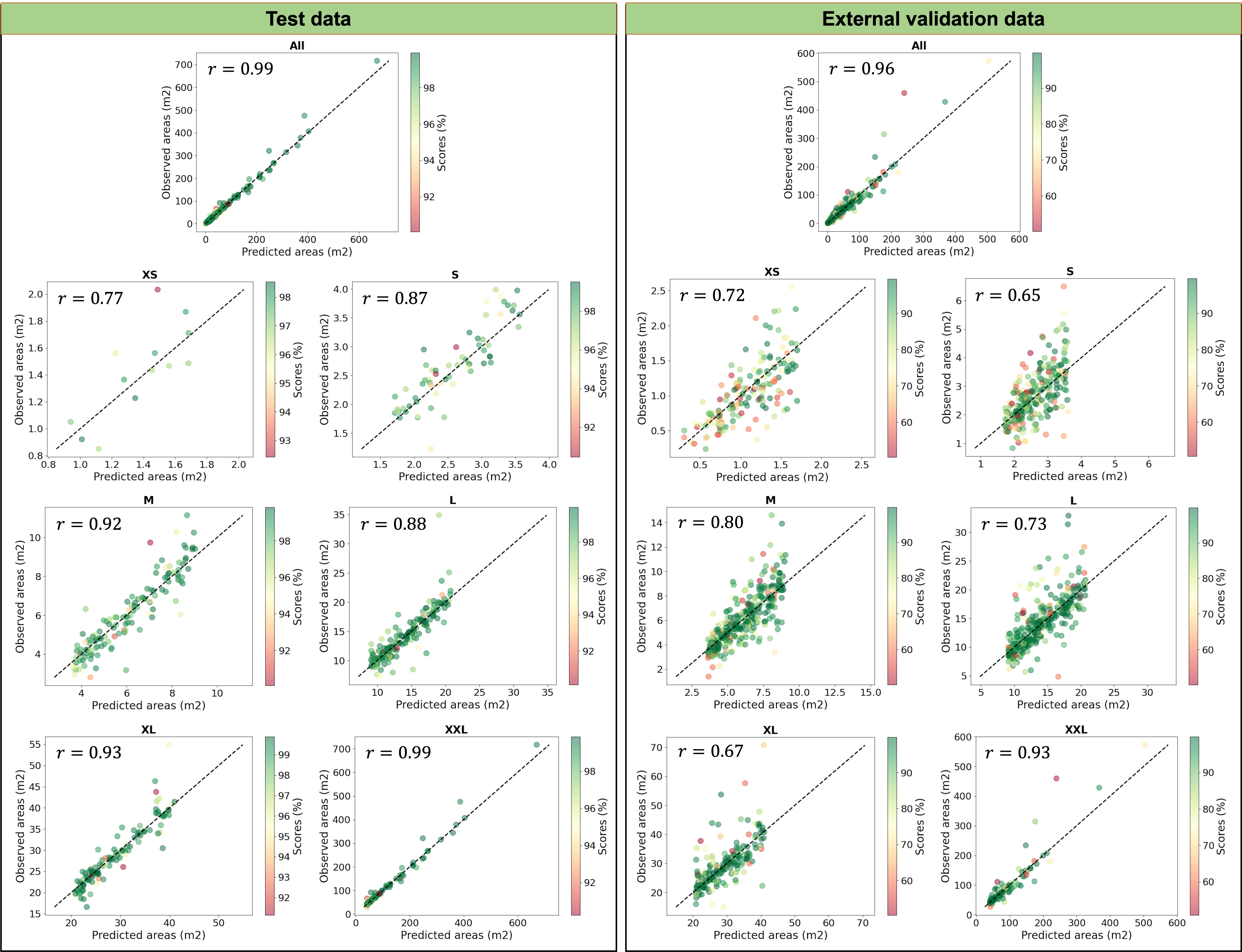
Figure 15: Correlations between real and predicted Juniperus areas over all shrub sizes and over the six size ranges: extra small (XS), small (S), medium (M), large (L), extra large (XL), and extra extra large (XXL) using $\theta_{MIoGTA}=50\%$. To the left the correlations within the test data are displayed at $\theta_{score}=90\%$. To the right the correlations within the external validation data are displayed at $\theta_{score}=50\%$. The color of the points refer to the magnitude of the confidence score $\theta_{score}$ given by the model to each shrub. $r$ is the Pearson correlation coefficient.

4.6 Analyzing the model deployment

In this section, we present the results of the model deployment process over the National Park of Sierra Nevada. We also analyze the model detections using different confidence score thresholds, multiple shrub size categories, and different topographical features: altitude, terrain slope, and terrain aspect.

Fig 16 displays the distribution of the detected Juniperus with respect to each confidence score threshold $\theta_{score}\in\{50\%,80\%,90\%,95\%,98\%,99\%\}$. We can observe that Juniperus are highly concentrated in the North-West region and follow a stripe pattern in the North-East region, while they are less concentrated in the Southern region. In addition, it is noteworthy that when the confidence score threshold increases the number of shrubs per hectare decreases ranging from a maximum number of 152 shrubs per hectare with $\theta_{score}=50\%$, to 78 shrubs per hectare with $\theta_{score}=90\%$, to 29 shrubs per hectare with $\theta_{score}=99\%$.

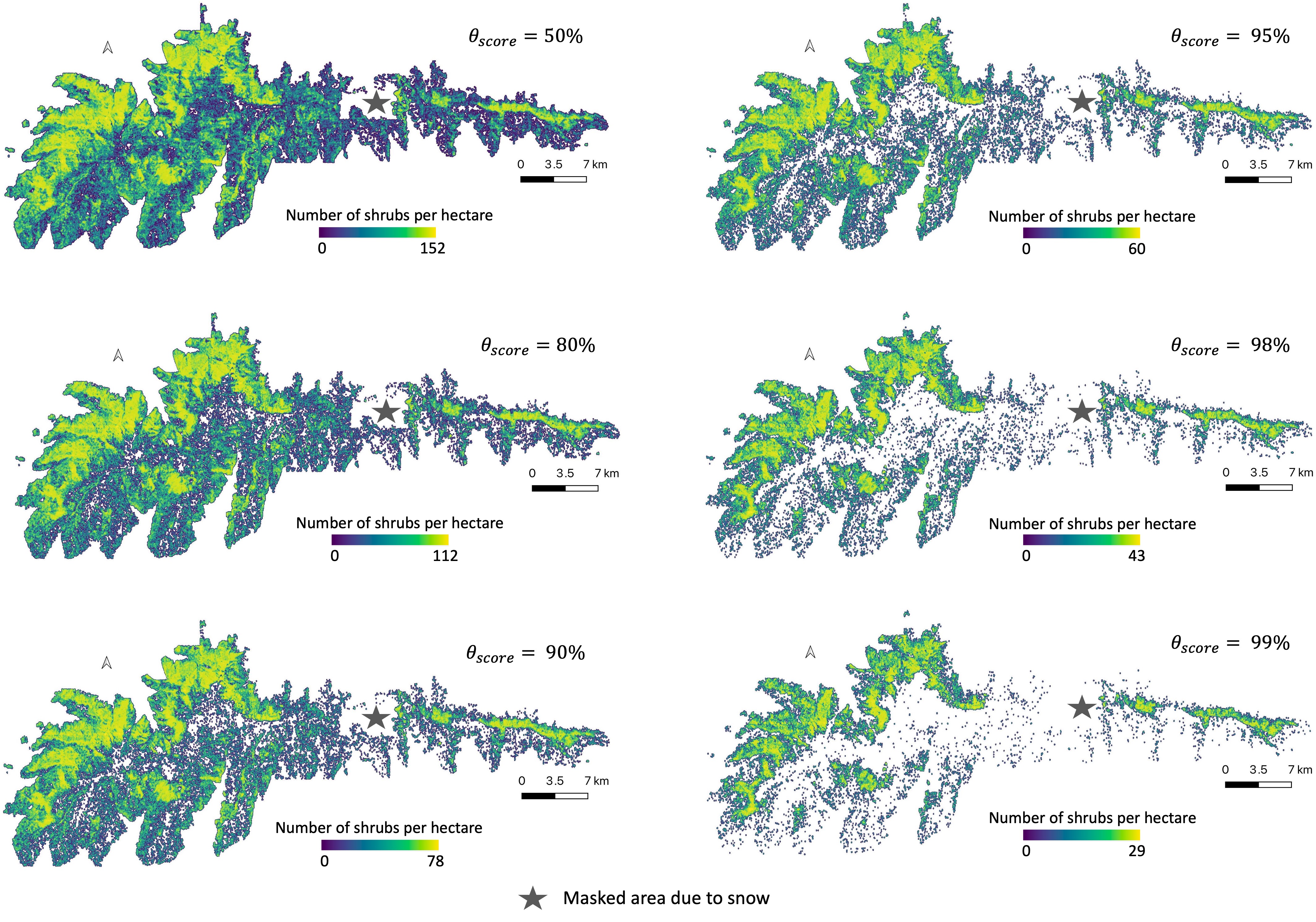
Figure 16: Density map highlighting the distribution of Juniperus, in the National Park of Sierra Nevada of Spain, with respect to each model’s confidence score threshold $\theta_{score}$ using an altitude threshold of 1900m.

In Fig. 17, we present the distribution of Juniperus shrubs for each altitude range from 1.9km to 3.5km with a step of 100m with respect to the aforementioned confidence score thresholds. For all the score thresholds the number of shrubs follows the same pattern: it increases until 2.5km of altitude, then starts to decrease gradually. In the same context, Fig. 18 displays the distribution of these shrubs for each shrub size category at $\theta_{score}=80\%$. Accordingly, they are more concentrated within a specific range of altitude (mainly between 2000 and 2600 m). In addition, we observe that the different shrub size categories follow an altitude-based order where small shrubs (XS, S, and M) have high tendency to grow at high altitudes (i.e, above 2375m) while large shrubs (XXL, XL, and L) grow at low altitudes (i.e., below 2375m). Furthermore, the shrubs are distributed as follows: there are 188,963 M-sized shrubs, 148,530 L-sized shrubs, 121,379 S-sized shrubs, 66,612 XL-sized shrubs, 50,949 XXL-sized shrubs, and 44,791 XS-sized shrubs.

To study the distribution of Juniperus with respect to terrain slopes, a slope map of the Sierra Nevada was generated from the DEM at 2m/pixel resolution. Fig. 19 exhibits the distribution of the different Juniperus size categories over all terrain slope ranges from 0 to 90 degrees at confidence score threshold $\theta_{score}=80\%$. Accordingly, all the categories of shrub sizes follow the same pattern and mostly grow between a slope of value 10 and 30 degrees (i.e., moderately steep slopes), while their number decreases exponentially after 30 degrees of slope.

Similarly, to study the distribution of Juniperus with respect to mountain orientation (i.e., aspect), a terrain aspect map of the Sierra Nevada was generated from the DEM at 2m/pixel resolution. Fig 20 depicts the distribution of the different Juniperus size categories over all terrain orientations at confidence score threshold $\theta_{score}=80\%$. In accordance with Fig. 16, most shrubs are highly concentrated in the North-West slopes and less concentrated in the South and South-East slopes. Fig. 20 also displays that there is a relatively higher proportion of small shrubs in the East orientation compared to the other shrub sizes.

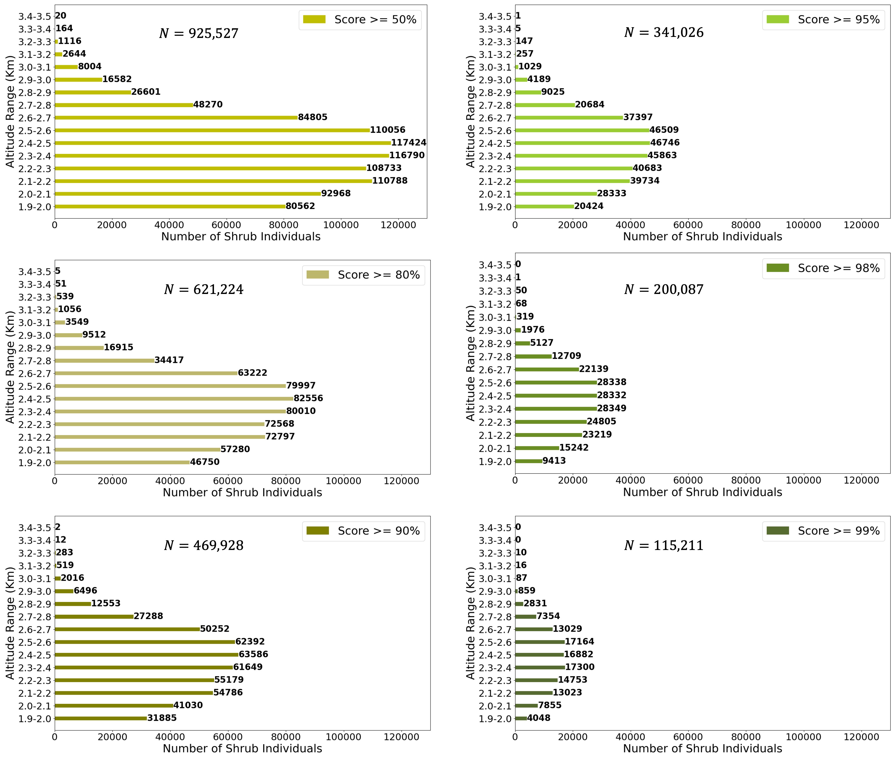
Figure 17: Distribution of the total number of Juniperus over all altitude ranges from 1.9km to 3.5km with respect to each model’s confidence score threshold $\theta_{score}$. $N$ is the total number of shrubs over all altitudes.

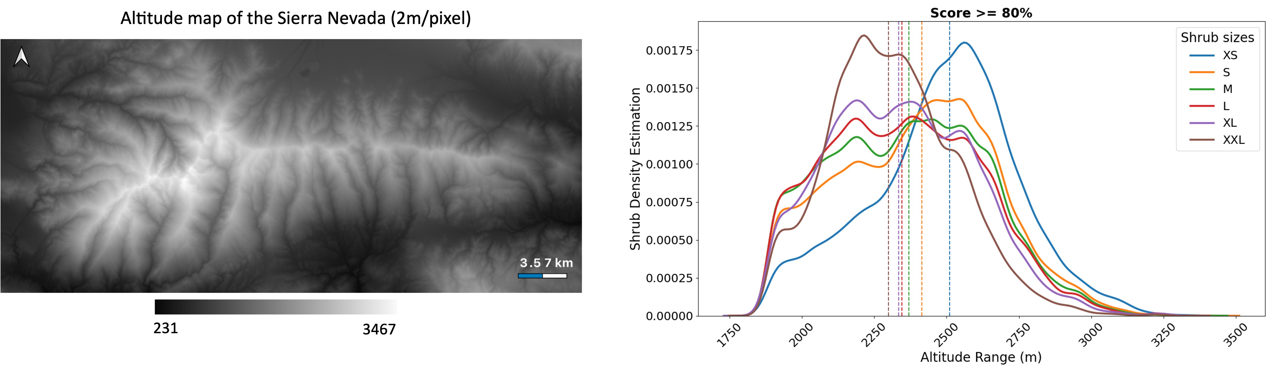
Figure 18: Density estimation of Juniperus sizes over all the different altitudes at model’s confidence score threshold $\theta_{score}=80\%$. The used shrub sizes are: extra small (XS), small (S), medium (M), large (L), extra large (XL), and extra extra large (XXL).

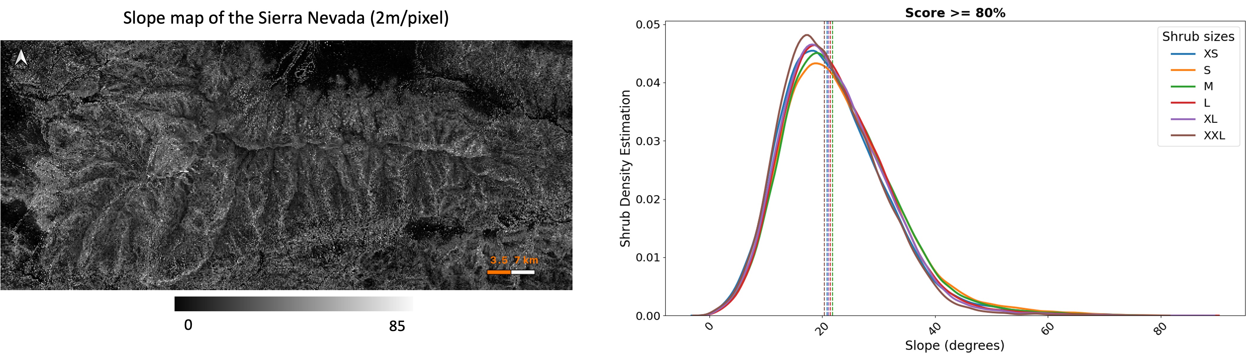
Figure 19: Density estimation of Juniperus sizes over all the different slopes at model’s confidence score threshold $\theta_{score}=80\%$. The used shrub sizes are: extra small (XS), small (S), medium (M), large (L), extra large (XL), and extra extra large (XXL).

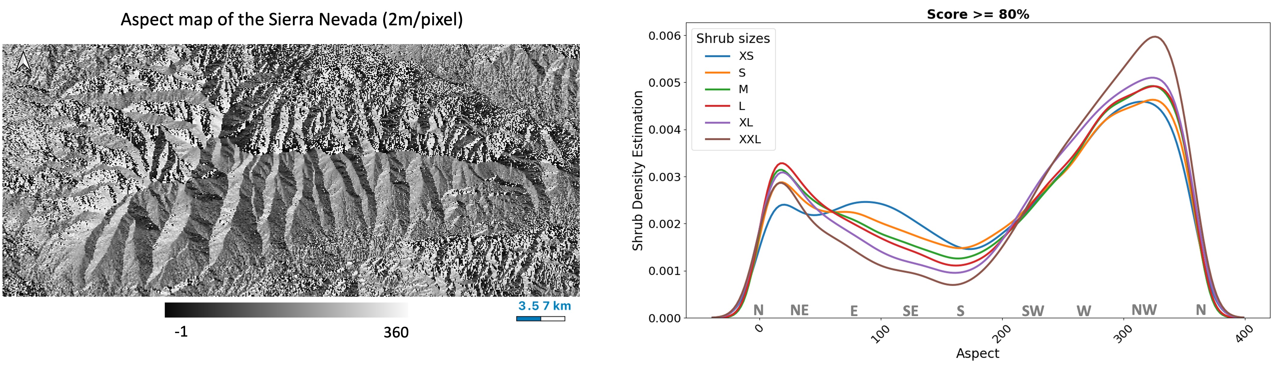
Figure 20: Distribution of Juniperus sizes over all the different types of terrain aspects (i.e., mountain orientation) at model’s confidence score threshold $\theta_{score}=80\%$. The used shrub sizes are: extra small (XS), small (S), medium (M), large (L), extra large (XL), and extra extra large (XXL). The aspect range for each orientation is: $NE\in[22.5,67.5[$, $E\in[67.5,112.5[$, $SE\in[112.5,157.5[$, $S\in[157.5,202.5[$, $SW\in[202.5,247.5[$, $W\in[247.5,292.5[$, $NW\in[292.5,337.5[$, and $N\in[0,22.5[\cup]337.5,370]$.

5 Discussion

5.1 Ecological considerations

Our methodology, which combines AI and RS technologies with the new data construction design and the new model evaluation protocol, was powerful to individually and accurately delineate Juniperus shrubs from RGB very-high-resolution satellite images in a complex mountain environment. Such a tool could be extended to systematically produce high-precision maps of Juniperus shrubs (or similar shrubs) in high-mountains or high latitudes to track climate change effects on their distribution, abundance, and size structure, and in the woody-line throughout the Palearctic.

This new tool makes it possible to count all the individuals present in a large geographic region (e.g. a mountain range), determining their size with a precision of 13x13 cm2. It allowed us to quantify the distribution, abundance and size (i.e., demographic structure) of individuals, which helped us to determine whether these population parameters varied as a function of environmental variables, such as altitude, slope, ecological context, etc., in mountain environments. In short, it allowed us to do things that are not possible with traditional field methodologies.

Our analysis showed that Juniperus are more abundant in the North-West region and in the North-West orientations of Sierra Nevada, within a specific range of altitude (mainly between 2000 and 2600 m), and on moderately steep slopes (mainly between 10 and 30 degrees). Our results also revealed a massive difference in shrub size with altitude, i.e., the distribution of small shrubs is biased towards the highest altitudes while the largest ones tend to occur at the lowest altitudes (Figure 19). Such dominance of the smallest individuals in the highest altitudes could be indicative of a process of altitudinal rise as a consequence of global warming, which requires further investigation using historical aerial photography. If this were the case, during the last decades, Juniperus communis individuals would have been establishing more successfully at higher altitudes, where they found the preferred temperature range, the necessary sunlight, and suitable habitats with less competition for resources with other plant species, and less human activity. The obtained results can be used to investigate the factors explaining Juniperus distribution, and can further be employed by policymakers to establish efficient management plans of this protected area.

5.2 Methodological considerations

We introduced a novel open-source dataset of very-high resolution RGB satellite images. This is the first DL-ready dataset of Juniperus species, and the largest of its kind in which 8580 shrubs were digitized (Guirado et al. 2017; 2021, James & Bradshaw 2020, Retallack et al. 2022). This is the first dataset for individual delineation of plants with complex growth patterns since all existing studies created datasets of plants with well defined and stable patterns and a straightforward spatial distribution where most of them are private or have restricted access (Zhang et al. 2020, Zheng et al. 2022, Kierdorf et al. 2023, Zheng et al. 2023, Gan et al. 2023, Sani-Mohammed et al. 2022). Our primary objective is to present a valuable resource for designing and developing DL models to individually delineate shrubs in particular, and plants with complex patterns in general.

DL models are known as data-hungry models (Adadi 2021, Christin et al. 2019). However, collecting data through field surveying is costly, laborious, time-consuming, unsustainable, and spatially restricted. To the best of our knowledge, a data design handling such issues is lacking in the literature, as existing studies developed and externally validated their models only on FW data (Guirado et al. 2017; 2021, James & Bradshaw 2020, Retallack et al. 2022). Thus, we proposed a new data construction approach (i.e., dual PI-FW data design) that consist in developing the model with PI dataset, then externally validating it using FW dataset. Our outcomes proved the efficiency and scalability of this approach in developing a delineation model in a more optimized way.

We proposed a new evaluation algorithm based on a new metric called MIoGTA to assess and optimize the delineation performance of instance segmentation models. Our results demonstrate the robustness of the proposed metric in reducing the FPs and FNs compared to the standard IoU metric. All existing studies delineating shrubs and other types of plants used the standard IoU metric to evaluate their models (James & Bradshaw 2020, Retallack et al. 2022, Zheng et al. 2023, Zhang et al. 2020, Gan et al. 2023, Kierdorf et al. 2023). However, natural species may have complex growth patterns (i.e., high variation in their spatial distribution) making the experts-based data annotation process prone to uncertainty. The IoU metric relies on the quality of data annotation and it was proved that using this metric in such cases generates an unfair and a non representative evaluation of the model performance. Therefore, our proposed metric overcomes the aforementioned limitations being less sensitive to data annotation uncertainty and more robust in evaluating delineation models over plants with complex growth patterns.

To the best of our knowledge, this is the first study exploring the potential of AI models to delineate individual plants with complex growth patterns since all existing studies handle the delineation of plants with well defined patterns (Zhang et al. 2020, Zheng et al. 2022; 2023, Gan et al. 2023, Sani-Mohammed et al. 2022).

This study is also the first attempt to deploy a DL model at the regional scale for individual delineation of high-mountain shrubs (Guirado et al. 2017; 2021, James & Bradshaw 2020, Retallack et al. 2022), simultaneously offering valuable insights into the distribution of these shrubs.

The proposed methodology can provide useful perspectives to the scientific community interested in using RS and AI technologies to individually delineate plants with complex growth patterns. The created data can open possibilities for new explorations of the potential of AI models and RS data for Earth observation. The developed model can be applied in other high-mountain ecosystems to individually delineate the same type of shrubs. It can also be applied to delineate other types of shrubs by fine tuning the model using small amount of data.

5.3 Limitations

Indeed, our model provides useful insights about shrubs distribution in high mountains, however, it still ignores some shrubs (FNs), and still makes some false detections (FPs). These FPs can be manifested in the detection of other kinds of shrubs, isolated trees, small dark rocks with shades, edges of lagoons, and parts of "borreguiles" (i.e., humid pastures/grasslands). On the other hand, FNs can be noticed when shrubs have aggregated growth patterns, when the shrub size is very large and covers a great proportion of the image tile size, when the image background is very dark, and when the land cover is very patchy.

These FPs and FNs are totally expected where the main factors explaining the high ability of the model to delineate shrubs in some areas while not in other areas can be summarized as follows:

1. The temporal distribution of satellite images which is related to the season during which these images were captured. Winter-based images are more likely to contain snow, the soils are darker than in summer-based images due to soil humidity, less sun light, and the existence of clouds and cloud shadows.

2. The spatial distribution of satellite images: images are captured from different angles that can introduce shadows from trees, hills, etc. Sometimes, they can have different resolutions where some areas are captured with very high resolution while others with less resolution.

3. The spectral resolution of satellite images: in the case of this study, only three visual bands (RGB) are used. Adding more spectral information may provide enough differentiation to help the model confusing rocks, lagoons, and humid grasslads with shrubs.

4. The local heterogeneity and patchiness of the area: areas with homogeneous land covers, such as barren lands, are easier for the model to detect shrubs than areas with high heterogeneity such as urban areas or cropland mosaics.

5. The complex growth patterns of Juniperus: these shrubs exhibit a significant variation in their spatial patterns and shape along their distribution. Although we tried to make our data representative of the different shapes and backgrounds, it is difficult to collect all aspect in nature of this multiple faces shrub.

6. The distribution of the PI dataset: given that the PI data relies on expert visual inspection of images, we excluded images featuring complex Juniperus behavior due to low expert confidence. This exclusion can prevent the model from being trained on images with more complex patterns.

To solve some of the aforementioned issues and further improve the model performance, ancillary information can be included such as orientation, altitude, and slope. For instance, stripe sized shrubs can only grow in areas with high slopes. Multispectral data can also be a good alternative to prevent the model from making false detections. In addition, other DL models architectures are encouraged to be evaluated.

6 Conclusion

In this study, we demonstrated the potential of combining remotely sensed RGB imagery with Mask R-CNN instance segmentation model using a new data construction design and a new model evaluation protocol to individually delineate Juniperus shrubs in high-mountain ecosystems.

Our deployment results revealed that the distribution of Juniperus shrubs is influenced by topographic features, including altitude, slope, and mountain orientation. Notably, these shrubs exhibit a pronounced concentration in the North-West region and in the North-West orientations of Sierra Nevada, within a specific range of altitude, and on moderately steep slopes. This concentration pattern reveals that currently smaller shrubs tend to occur at higher altitudes, while larger shrubs are more prevalent at lower altitudes. Such potential shift in the altitudinal range will be investigated in further research. Our work and cartography will assist to the management and conservation of the Sierra Nevada National Park, a global hotspot for biodiversity, in the face of global warming.

Our experimental results showed the efficiency of the proposed dual data construction approach (i.e., PI and FW) in overcoming the limitations associated with traditional field surveying methods. They also indicate the robustness of the proposed MIoGTA metric in evaluating the delineation ability of instance segmentation models on species with complex growth patterns showing a great resilience against the uncertainty of the data annotation process performed by experts. In addition, they demonstrated the potential of AI models in individually delineating plants with complex growth patterns. Particularly, they showed the effectiveness of employing Mask R-CNN with ResNet101-C4 backbone in delineating both PI and FW shrubs achieving F1-score of 87,87% and 76.86%, respectively. However, the results captured a drop in the model performance to delineate XS shrubs compared to other shrub sizes.

While this study marks a significant advancement in the application of RS and DL for individual shrub delineation, it is important to acknowledge its limitations. The delineation accuracy is influenced by several factors, including the temporal and spatial distribution of satellite images, the spectral resolution of satellite images, the heterogeneity of the background, the complex growth patterns of Juniperus shrubs, and the distribution of the PI data used to develop the delineation model. Future studies should focus on refining these aspects to achieve even greater accuracy by using ancillary information (topographic, atmospheric, etc.), multispectral data, and new delineation models.

Declaration of Competing Interest

The authors declare that they have no known competing financial interests or personal relationships that could have appeared to influence the work reported in this paper.

Data availability

Data will be made available to the public after the acceptation of the paper.

Code availability

The scripts used to perform this study will be made avaiable to the public after the acceptation of the paper.

Appendix A

Algorithm 1 Description of the IoU-based evaluation algorithm

1:  Inputs: The set of predictions $S_{p}$ obtained after applying a confidence score threshold $\theta_{score}$: $S_{p}=\{p_{i}:i\in[1:n]\}$ The set of labels $S_{l}$: $S_{l}=\{l_{j}:j\in[1:m]\}$ The evaluation metric $IoU$ and its threshold $\theta_{IoU}$.

2:  Outputs: The number of TP, FP, and FN: $\{n_{TP},n_{FP},n_{FN}\}$

3:  Initialize $n_{TP}\leftarrow 0$ , $n_{FP}\leftarrow 0$ and $n_{FN}\leftarrow 0$

4:  for each prediction $p_{i}$ in $S_{p}$ do

5:     Find the best match label $l_{match}$ with the prediction $p_{i}$

6:     Compute the evaluation metric $IoU(p_{i},l_{match})$

7:     if $IoU(p_{i},l_{match})\geq\theta_{IoU}$ then

8:        $n_{TP}\leftarrow 1$

9:     else

10:        $n_{FP}\leftarrow 1$

11:     end if

12:  end for

13:  for each label $l_{j}$ in $S_{l}$ do

14:     Find the best match prediction $p_{match}$ with the label $l_{j}$

15:     Compute the evaluation metric $IoU(l_{j},p_{match})$

16:     if $IoU(l_{j},p_{match})<\theta_{IoU}$ then

17:        $n_{FN}\leftarrow 1$

18:     end if

19:  end for

Algorithm 2 Description of the MIoGTA-based evaluation algorithm

1:  Inputs: The set of predictions $S_{p}$ obtained after applying a confidence score threshold $\theta_{score}$: $S_{p}=\{p_{i}:i\in[1:n]\}$ The set of labels $S_{l}$: $S_{l}=\{l_{j}:j\in[1:m]\}$ The evaluation metric $MIoGTA$ and its threshold $\theta_{MIoGTA}$.

2:  Outputs: The number of TP, FP, and FN: $\{n_{TP},n_{FP},n_{FN}\}$

3:  Initialize $n_{TP}\leftarrow 0$ , $n_{FP}\leftarrow 0$ and $n_{FN}\leftarrow 0$

4:  for each prediction $p_{i}$ in $S_{p}$ do

5:     Find the set of labels $S_{l_{match}}\subset S_{l}$ matching with the prediction $p_{i}$

6:     Compute the evaluation metric $MIoGTA(p_{i},S_{l_{match}})$

7:     if $MIoGTA(p_{i},S_{l_{match}})\geq\theta_{MIoGTA}$ then

8:        $n_{TP}\leftarrow 1$

9:     else

10:        $n_{FP}\leftarrow 1$

11:     end if

12:  end for

13:  for each label $l_{j}$ in $S_{l}$ do

14:     Find the set of predictions $S_{p_{match}}\subset S_{p}$ matching with the label $l_{j}$

15:     Compute the evaluation metric $MIoGTA(l_{j},S_{p_{match}})$

16:     if $MIoGTA(l_{j},S_{p_{match}})<\theta_{MIoGTA}$ then

17:        $n_{FN}\leftarrow 1$

18:     end if

19:  end for

References

- Adadi (2021) Adadi, A. (2021). A survey on data-efficient algorithms in big data era. Journal of Big Data, 8, 24.
- Adhikari et al. (2017) Adhikari, A., Yao, J., Sternberg, M., McDowell, K., & White, J. D. (2017). Aboveground biomass of naturally regenerated and replanted semi-tropical shrublands derived from aerial imagery. Landscape and Ecological Engineering, 13, 145–156.
- Ayhan & Kwan (2020) Ayhan, B., & Kwan, C. (2020). Tree, shrub, and grass classification using only rgb images. Remote Sensing, 12, 1333.
- Ayhan et al. (2020) Ayhan, B., Kwan, C., Budavari, B., Kwan, L., Lu, Y., Perez, D., Li, J., Skarlatos, D., & Vlachos, M. (2020). Vegetation detection using deep learning and conventional methods. Remote Sensing, 12, 2502.
- Bellard et al. (2012) Bellard, C., Bertelsmeier, C., Leadley, P., Thuiller, W., & Courchamp, F. (2012). Impacts of climate change on the future of biodiversity. Ecology letters, 15, 365–377.
- Carvalho et al. (2020) Carvalho, O. L. F. d., de Carvalho Junior, O. A., Albuquerque, A. O. d., Bem, P. P. d., Silva, C. R., Ferreira, P. H. G., Moura, R. d. S. d., Gomes, R. A. T., Guimaraes, R. F., & Borges, D. L. (2020). Instance segmentation for large, multi-channel remote sensing imagery using mask-rcnn and a mosaicking approach. Remote Sensing, 13, 39.
- Chai et al. (2021) Chai, J., Zeng, H., Li, A., & Ngai, E. W. (2021). Deep learning in computer vision: A critical review of emerging techniques and application scenarios. Machine Learning with Applications, 6, 100134.
- Champ et al. (2020) Champ, J., Mora-Fallas, A., Goëau, H., Mata-Montero, E., Bonnet, P., & Joly, A. (2020). Instance segmentation for the fine detection of crop and weed plants by precision agricultural robots. Applications in plant sciences, 8, e11373.
- Christin et al. (2019) Christin, S., Hervet, É., & Lecomte, N. (2019). Applications for deep learning in ecology. Methods in Ecology and Evolution, 10, 1632–1644.
- Dong et al. (2019) Dong, T., Shen, Y., Zhang, J., Ye, Y., & Fan, J. (2019). Progressive cascaded convolutional neural networks for single tree detection with google earth imagery. Remote Sensing, 11, 1786.
- El-Barougy et al. (2023) El-Barougy, R. F., Dakhil, M. A., Halmy, M. W. A., Cadotte, M., Dias, S., Farahat, E. A., El-keblawy, A., & Bersier, L.-F. (2023). Potential extinction risk of juniperus phoenicea under global climate change: Towards conservation planning. Global Ecology and Conservation, (p. e02541).
- Gan et al. (2023) Gan, Y., Wang, Q., & Iio, A. (2023). Tree crown detection and delineation in a temperate deciduous forest from uav rgb imagery using deep learning approaches: Effects of spatial resolution and species characteristics. Remote Sensing, 15, 778.
- García et al. (2000) García, D., Zamora, R., Gómez, J. M., Jordano, P., & Hódar, J. A. (2000). Geographical variation in seed production, predation and abortion in juniperus communis throughout its range in europe. Journal of Ecology, 88, 435–446.
- García et al. (1999) García, D., Zamora, R., Hódar, J. A., & Gómez, J. M. (1999). Age structure of juniperus communis l. in the iberian peninsula: conservation of remnant populations in mediterranean mountains. Biological Conservation, 87, 215–220.
- Gené-Mola et al. (2020) Gené-Mola, J., Sanz-Cortiella, R., Rosell-Polo, J. R., Morros, J.-R., Ruiz-Hidalgo, J., Vilaplana, V., & Gregorio, E. (2020). Fruit detection and 3d location using instance segmentation neural networks and structure-from-motion photogrammetry. Computers and Electronics in Agriculture, 169, 105165.
- Guirado et al. (2021) Guirado, E., Blanco-Sacristan, J., Rodriguez-Caballero, E., Tabik, S., Alcaraz-Segura, D., Martinez-Valderrama, J., & Cabello, J. (2021). Mask r-cnn and obia fusion improves the segmentation of scattered vegetation in very high-resolution optical sensors. Sensors, 21, 320.
- Guirado et al. (2017) Guirado, E., Tabik, S., Alcaraz-Segura, D., Cabello, J., & Herrera, F. (2017). Deep-learning versus obia for scattered shrub detection with google earth imagery: Ziziphus lotus as case study. Remote Sensing, 9, 1220.
- He et al. (2017) He, K., Gkioxari, G., Dollár, P., & Girshick, R. (2017). Mask r-cnn. In Proceedings of the IEEE international conference on computer vision (pp. 2961–2969).
- James & Bradshaw (2020) James, K., & Bradshaw, K. (2020). Detecting plant species in the field with deep learning and drone technology. Methods in Ecology and Evolution, 11, 1509–1519.
- James & Bradshaw (2021) James, K., & Bradshaw, K. (2021). Shrub detection in high-resolution imagery: A comparative study of two deep learning approaches. In International Advanced Computing Conference (pp. 545–561). Springer.
- Khaldi & Shah (2021) Khaldi, K., & Shah, S. K. (2021). Cupr: Contrastive unsupervised learning for person re-identification. In VISIGRAPP (5: VISAPP) (pp. 92–100).
- Kierdorf et al. (2023) Kierdorf, J., Junker-Frohn, L. V., Delaney, M., Olave, M. D., Burkart, A., Jaenicke, H., Muller, O., Rascher, U., & Roscher, R. (2023). Growliflower: An image time-series dataset for growth analysis of cauliflower. Journal of Field Robotics, 40, 173–192.
- Krebs (2013) Krebs, C. (2013). Ecology: The Experimental Analysis of Distribution and Abundance. Always learning. Pearson. URL: https://books.google.es/books?id=Rq5GngEACAAJ.
- Li et al. (2021) Li, Z., Ding, J., Zhang, H., & Feng, Y. (2021). Classifying individual shrub species in uav images—a case study of the gobi region of northwest china. Remote Sensing, 13, 4995.
- Lin et al. (2014) Lin, T.-Y., Maire, M., Belongie, S., Hays, J., Perona, P., Ramanan, D., Dollár, P., & Zitnick, C. L. (2014). Microsoft coco: Common objects in context. In Computer Vision–ECCV 2014: 13th European Conference, Zurich, Switzerland, September 6-12, 2014, Proceedings, Part V 13 (pp. 740–755). Springer.
- Madsen et al. (2020) Madsen, B., Treier, U. A., Zlinszky, A., Lucieer, A., & Normand, S. (2020). Detecting shrub encroachment in seminatural grasslands using uas lidar. Ecology and Evolution, 10, 4876–4902.
- Nguyen et al. (2024) Nguyen, V. D., Khaldi, K., Nguyen, D., Mantini, P., & Shah, S. (2024). Contrastive viewpoint-aware shape learning for long-term person re-identification. In Proceedings of the IEEE/CVF Winter Conference on Applications of Computer Vision (pp. 1041–1049).
- Niphadkar et al. (2017) Niphadkar, M., Nagendra, H., Tarantino, C., Adamo, M., & Blonda, P. (2017). Comparing pixel and object-based approaches to map an understorey invasive shrub in tropical mixed forests. Frontiers in plant science, 8, 892.
- Otto et al. (2012) Otto, F. E., Massey, N., van Oldenborgh, G. J., Jones, R. G., & Allen, M. R. (2012). Reconciling two approaches to attribution of the 2010 russian heat wave. Geophysical Research Letters, 39.
- Palacios et al. (2020) Palacios, D., Oliva, M., Gómez-Ortiz, A., Andrés, N., Fernández-Fernández, J. M., Schimmelpfennig, I., Léanni, L., Team, A. et al. (2020). Climate sensitivity and geomorphological response of cirque glaciers from the late glacial to the holocene, sierra nevada, spain. Quaternary Science Reviews, 248, 106617.
- Retallack et al. (2022) Retallack, A., Finlayson, G., Ostendorf, B., & Lewis, M. (2022). Using deep learning to detect an indicator arid shrub in ultra-high-resolution uav imagery. Ecological Indicators, 145, 109698.
- Sani-Mohammed et al. (2022) Sani-Mohammed, A., Yao, W., & Heurich, M. (2022). Instance segmentation of standing dead trees in dense forest from aerial imagery using deep learning. ISPRS Open Journal of Photogrammetry and Remote Sensing, 6, 100024.
- Soubry et al. (2022) Soubry, I., Robinov, L., Chu, T., & Guo, X. (2022). Mapping shrub cover in grasslands with an object-based approach and investigating the connection to topo-edaphic factors. Geocarto International, 37, 16926–16950.
- Sun et al. (2022) Sun, Y., Li, Z., He, H., Guo, L., Zhang, X., & Xin, Q. (2022). Counting trees in a subtropical mega city using the instance segmentation method. International Journal of Applied Earth Observation and Geoinformation, 106, 102662.
- Thompson (2006) Thompson, A. (2006). Management under anarchy: the international politics of climate change. Climatic Change, 78, 7–29.
- Tian et al. (2020) Tian, Y., Yang, G., Wang, Z., Li, E., & Liang, Z. (2020). Instance segmentation of apple flowers using the improved mask r–cnn model. Biosystems engineering, 193, 264–278.
- Townsend et al. (2003) Townsend, C. R., Begon, M., Harper, J. L. et al. (2003). Essentials of ecology.. Ed. 2. Blackwell Science.
- Voulodimos et al. (2018) Voulodimos, A., Doulamis, N., Doulamis, A., Protopapadakis, E. et al. (2018). Deep learning for computer vision: A brief review. Computational intelligence and neuroscience, 2018.
- Weiss et al. (2016) Weiss, K., Khoshgoftaar, T. M., & Wang, D. (2016). A survey of transfer learning. Journal of Big data, 3, 1–40.
- Zhang et al. (2020) Zhang, C., Atkinson, P. M., George, C., Wen, Z., Diazgranados, M., & Gerard, F. (2020). Identifying and mapping individual plants in a highly diverse high-elevation ecosystem using uav imagery and deep learning. ISPRS Journal of Photogrammetry and Remote Sensing, 169, 280–291.
- Zheng et al. (2022) Zheng, C., Abd-Elrahman, A., Whitaker, V. M., & Dalid, C. (2022). Deep learning for strawberry canopy delineation and biomass prediction from high-resolution images. Plant Phenomics, .
- Zheng et al. (2023) Zheng, J., Yuan, S., Wu, W., Li, W., Yu, L., Fu, H., & Coomes, D. (2023). Surveying coconut trees using high-resolution satellite imagery in remote atolls of the pacific ocean. Remote Sensing of Environment, 287, 113485.