The Metallicity-Electron Temperature Relationship in H ii Regions

Abstract

H ii region heavy-element abundances throughout the Galactic disk provide important constraints to theories of the formation and evolution of the Milky Way. In LTE, radio recombination line (RRL) and free-free continuum emission are accurate extinction-free tracers of the H ii region electron temperature. Since metals act as coolants in H ii regions via the emission of collisionally excited lines, the electron temperature is a proxy for metallicity. Shaver et al. found a linear relationship between metallicity and electron temperature with little scatter. Here, we use CLOUDY H ii region simulations to (1) investigate the accuracy of using RRLs to measure the electron temperature; and (2) explore the metallicity-electron temperature relationship. We model 135 H ii regions with different ionizing radiation fields, densities, and metallicities. We find that electron temperatures derived under the assumption of LTE are about 20% systematically higher due to non-LTE effects, but overall LTE is a good assumption for cm-wavelength RRLs. Our CLOUDY simulations are consistent with the Shaver et al. metallicity-electron temperature relationship but there is significant scatter since earlier spectral types or higher electron densities yield higher electron temperatures. Using RRLs to derive electron temperatures assuming LTE yields errors in the predicted metallicity as large as 10%. We derive correction factors for Log(O/H) + 12 in each CLOUDY simulation. For lower metallicities the correction factor depends primarily on the spectral-type of the ionizing star and range from 0.95 to 1.10, whereas for higher metallicities the correction factor depends on the density and is between 0.97 and 1.05.

1 Introduction

H ii regions are the sites of massive star formation where O and B-type stars ionize the surrounding gas (Strömgren, 1939). Since H ii regions are short-lived ($\lesssim 10$$\,{\rm Myr}$), their elemental abundances correspond to present-day values at their location in the Galaxy. They therefore provide a snapshot of the distribution of elemental abundances that are critical to constrain Galactic chemical evolution models (e.g., Chiappini et al., 2001). H ii region abundance studies complement similar studies of stars, which are typically much older and have moved from their birthplace (e.g., Schönrich & Binney, 2009).

H ii regions are bright at multiple wavelengths. They emit copious amounts of energy via collisionaly excited lines (CELs) from metals at optical (e.g., Peimbert & Costero, 1969) and infrared (e.g., Simpson et al., 1995) wavelengths, and they are detected in radio recombination line (RRL) and continuum emission (Hoglund & Mezger, 1965). H ii region tracers at radio wavelengths have the advantage that they are not affected by dust and can be detected throughout the Galactic disk. Recently, H ii region RRL surveys have nearly tripled the number of known Galactic H ii regions (Anderson et al., 2011; Wenger et al., 2021).

For an optically thin nebula in local thermodynamic equilibrium (LTE), the RRL and free-free continuum ratio provides an excellent probe of the electron (thermal) temperature (e.g., Wilson et al., 2009). In LTE, both the RRL emission and continuum emission have the same dependence on electron density, but differ in their dependence on electron temperature. Furthermore, since we are forming a line-to-continuum ratio there is no need for an absolute calibration of the intensity scale, yielding a very accurate determination of the electron temperature. In particular, radio interferometers provide very precise measurements of the line-to-continuum ratio yielding electron temperatures with uncertainties of $\sim 1$% (Wenger et al., 2019). Systematic uncertainties should therefore dominate (e.g., non-LTE effects).

Churchwell & Walmsley (1975) were the first to use RRL and continuum data toward a sample of Galactic H ii regions to discover radial electron temperature gradients in the Milky Way disk (also see Lichten et al., 1979). They suggested that these results were due to radial metallicity gradients, similar to those found by observations of optical CELs in nearby galaxies (Searle, 1971). Theoretical models of H ii regions predict that the metal abundance is the dominant factor that determines the electron temperature (e.g., Rubin, 1985). This is because metals act as coolants via the escape of CEL radiation from primarily oxygen and nitrogen (e.g., Osterbrock & Ferland, 2006).

Shaver et al. (1983) derived an empirical metallicity-electron temperature relationship by using optical CELs of oxygen to determine the O/H abundance ratio, and RRLs to determine the electron temperature, $T_{\rm e}$, toward a sample of Galactic H ii regions. Since RRLs of elements heavier than hydrogen and helium are too weak to detect in H ii regions, using the electron temperature as a proxy for metallicity provides an indirect method to explore metallicity structure in the Milky Way disk with radio data. Recent results of this technique have found azimuthal metallicity structure in the Galactic disk in addition to the well-established radial metallicity gradient (Balser et al., 2011, 2015; Wenger et al., 2019).

Factors other than metallicity that affect the electron temperature may not be negligible, however, and should be considered when evaluating the metallicity-electron temperature relationship. For example, the stellar effective temperature, $T_{\rm eff}$, of the ionizing star determines the hardness of the radiation field that excites and heats the gas, so higher values of $T_{\rm eff}$ will marginally increase $T_{\rm e}$ (Rubin, 1985). The electron density, $n_{\rm e}$, alters the rate of collisional de-excitation and so higher values of $n_{\rm e}$ will inhibit cooling and thus slightly increase $T_{\rm e}$ (Rubin, 1985). Lastly, dust affects the electron temperature in complex ways (Mathis, 1986; Baldwin et al., 1991; Shields & Kennicutt, 1995). Dust can enable heating through the photo-electric effect as electrons are ejected from dust grains and collide with atoms. In contrast, cooling can result when there are collisions of fast particles with dust grains.

2 Cloudy Simulations

Here, we investigate the metallicity-electron temperature relationship by simulating H ii regions using the spectral synthesis code CLOUDY (Chatzikos et al., 2023). We model a wide range of H ii regions physical conditions and investigate departures from LTE in RRL emission. We use a development version of CLOUDY (trunk branch, revision r13270M) that includes an update to the energy changing collisonal rates that is important for predicting RRL emission from ionized gas (for details see Guzmán et al., 2019). For all simulations we assume a spherical nebula with hydrogen density, $n_{\rm H}$, and diameter, $D$, ionized by a central star. Since we are modeling spectral transitions with high principal quantum number, $n$, a large number of quantum levels must be considered. The first 25 levels from hydrogen are resolved into $nl$ terms, whereas the next 375 levels are collapsed into one effective level where the $nl$ terms are assumed to be populated according to their statistical weight. Here, $l$ is the azimuthal quantum number related to the angular momentum of the atom. All simulations use the semiclassical straight-trajectory Born approximation of Lebedev & Beigman (1998) for the excitation rate coefficients as recommended by Guzmán et al. (2019).

We use CLOUDY to explore the wide range of physical properties found in Galactic H ii regions. Table 1 summarizes the H ii region properties of the CLOUDY simulations. We choose three different spectral types—O3, O6, and O9—in our grid of simulations with corresponding effective temperatures and number of H-ionizing photons, $N_{\rm Ly}$, given by Martins et al. (2005). We use the ATLAS stellar grids which are LTE, plane-parallel, hydrostatic model atmospheres (Castelli & Kurucz, 2003). We assume the metallicity of the star and gas are the same and therefore select the stellar metallicity that is closest to the gas metallicity (see below). There are some nearby H ii regions that are ionized by B-type stars, but most H ii regions detected at optical or radio wavelengths require O-type stars (e.g., Caplan et al., 2000; Bania et al., 2007).

Kurtz (2005) classifies H ii regions based on their density and size. We approximately follow this classification in our grid of simulations by modeling ultra-compact to giant H ii regions. This sets the total hydrogen density and size of the model nebula where more compact sources will have higher densities. The range of ($n_{\rm H},D$) pairs corresponds to emission measures $EM\equiv\int{n_{\rm e}^{2}d\ell}=10^{3}-10^{7}$$\,{\rm cm^{-6}\,pc}$ for a fully ionized nebula. We therefore call these ($n_{\rm H},D$) pairs EM3, EM4, etc. (see Table 1).

The nominal elemental abundance ratios relative to hydrogen are specified by the CLOUDY H ii region model for Orion. The abundances are determined by calculating the mean value from three independent studies. We vary the metallicity via the CLOUDY metals command which scales the abundance ratios for all elements heavier than helium. This corresponds to O/H abundance ratios between Log(O/H) + 12 = 7.8 and 9.4 that conservatively encompasses the values determined across the Milky Way disk (e.g., Deharveng et al., 2000; Rudolph et al., 2006; Arellano-Córdova et al., 2020, 2021). We do not include dust for two reasons. First, Oliveira & Maciel (1986) estimate that the net effect of dust on the electron temperature is relatively small. Second, for some simulations that included Orion dust grains, we received warnings that the dust would not survive at these temperatures and thus the simulations were not realistic.

Table 1: CLOUDY Simulation H ii Region Properties

Ionizing Star				Cloud Properties				Metallicity
Spectral	$T_{\rm eff}$	Log($N_{\rm Ly}$)		$n_{\rm H}$	$D$	Name		Log(O/H) + 12
Type	(K)	(s-1)		(cm-3)	(pc)
O3	44,616	49.63		10	10.0	EM3		7.8
O6	38,151	48.63		50	4.0	EM4		8.0
O9	31,524	47.90		200	2.5	EM5		8.2
$\cdots$	$\cdots$	$\cdots$		1,000	1.0	EM6		8.4
$\cdots$	$\cdots$	$\cdots$		10,000	0.1	EM7		8.6
$\cdots$	$\cdots$	$\cdots$		$\cdots$	$\cdots$	$\cdots$		8.8
$\cdots$	$\cdots$	$\cdots$		$\cdots$	$\cdots$	$\cdots$		9.0
$\cdots$	$\cdots$	$\cdots$		$\cdots$	$\cdots$	$\cdots$		9.2
$\cdots$	$\cdots$	$\cdots$		$\cdots$	$\cdots$	$\cdots$		9.4

Note. — The CLOUDY simulations consider 3 different spectral types with corresponding effective temperature ($T_{\rm eff}$) and hydrogen ionizing photon rates ($N_{\rm Ly}$); 5 different spherical nebulae with density ($n_{\rm H}$) and diameter ($D$); and 9 different metallicities characterized by the O/H abundance ratio. This corresponds to $3\times 5\times 9=135$ simulations.

What is the optimal RRL transition to observe when using radio data to determine the electron temperature? To derive accurate electron temperatures requires (1) that the RRL and free-free continuum emission be optically thin; and (2) that the RRL be formed in LTE. To accommodate (1) in classical H ii regions the RRL frequency must be greater than about 5$\,{\rm GHz}$ or Hn$\alpha$ transitions with $n\lesssim 109$ (e.g., Wilson et al., 2009). RRL emission from most Galactic H ii regions is typically close to LTE. This is because the physical conditions necessary for non-LTE effects, low electron densities and high emission measure, are not common in Galactic H ii regions (see Shaver, 1980a). This depends, however, on the detailed physical conditions, geometry, and RRL frequency. For example, significant stimulated emission was found toward MWC 349, which may comprise of a rotating and expanding disk, from the H30$\alpha$ transition at 1$\,{\rm mm}$ (Martin-Pintado et al., 1989). Pressure broadening from electron impacts that decrease the peak line intensity was detected toward Sgr B2, which contains many high emission measure components, from the H109$\alpha$ transition at 6$\,{\rm cm}$ (von Procházka et al., 2010). Shaver (1980b) has determined that the optimal frequency to observe RRLs such that the electron temperature derived assuming LTE is equal to the true electron temperature is given by:

$$\nu\sim 0.081\,EM^{0.36}\,\,\,{\rm GHz}.$$ (1)

For typical Galactic H ii region emission measures this corresponds to cm-wavelength RRLs. This is, in part, why recent studies of Galactic metallicity structure have used cm-wavelength RRLs (Wenger et al., 2019). Here, we therefore focus on the H87$\alpha$ transition at 3.05$\,{\rm cm}$ as a representative RRL.

In total there are 135 CLOUDY simulations which correspond to 3 spectral types $\times$ 5 emission measures $\times$ 9 metallicities. Appendix A includes the input parameters for one CLOUDY simulation as an example. The simulations were run on an Intel Xeon Silver 4114 processor at 2.20$\,{\rm GHz}$. We only used 1 of the available 20 cores since the total memory (RAM) was only 251.4 GB and each simulation required $\sim 100\,$GB. Because of the large number of quantum levels that were considered each simulation took about 2.5 hr to run.

3 Results

All 135 CLOUDY simulations exited without errors after two iterations. The nebula was typically divided into about 200 numerical zones. For some simulations with high metallicities the nebular electron temperature fell below 4,000$\,{\rm K}$, the default threshold value below which the CLOUDY calculation will be stopped. This is the default value because thermal instabilities may occur when the temperature is below $\sim\rm few\times 10^{3}$$\,{\rm K}$ since the cooling curve allows more than one thermal solution (Williams, 1967). We therefore reran all simulations with a threshold temperature of 1,000$\,{\rm K}$ to allow for more realistic electron temperatures. For 30 simulations we lowered the threshold temperature to 500$\,{\rm K}$ because the temperature dropped below 1,000$\,{\rm K}$ halting the simulation. We received no warnings from CLOUDY that the heating-cooling balance was not preserved in these cases and therefore the temperatures should be reliable.

Figure 1 shows the incident and transmitted continuum for three representative simulations. As expected the simulations with earlier spectral type stars have harder incident radiation fields. The transmitted continuum includes emission from spectral lines. Notable are the CELs at infrared and optical frequencies. The RRLs are present but not visible on this scale.

Figure 2 illustrates how several physical properties vary with depth into the nebula for the same three simulations as shown in Figure 1. Included are the H ii and He ii ionization fraction and the electron temperature and density. The nebulae ionized by either O3 or O6-type stars are density-bounded where the hydrogen and helium are fully ionized. In contrast, the nebula ionized by the O9 star is ionization-bounded where neutral gas lies beyond the ionized gas. The electron temperature and density are relatively constant with depth but there are some variations. For example, the electron temperature slightly increases at the H ii region boundary because of photon hardening (e.g., Osterbrock & Ferland, 2006; Wilson et al., 2015). The electron density decreases past the He ii region boundary since fewer electrons are available from helium.

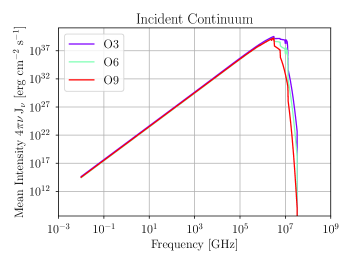
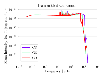
Figure 1: Incident and transmitted continuum spectra for three CLOUDY simulations. For all three simulations: $n_{\rm H}=200$$\,{\rm cm^{-3}}$, $D=2.5$$\,{\rm pc}$, and Log(O/H) + 12 = 8.6. This corresponds to an emission measure of $EM=10^{5}$$\,{\rm cm^{-6}\,pc}$ for a fully ionized nebula. Each plot shows the results for ionizing stars with spectral-types O3, O6, and O9. The transmitted continuum emission includes the spectral lines which are dominated by infrared and optical collisionally exited lines. At lower frequencies RRLs are present but not visible on this scale.

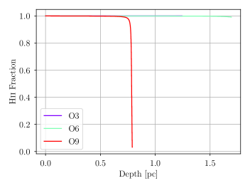
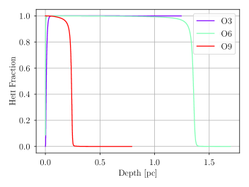
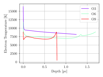
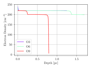
Figure 2: Physical properties as a function of nebula depth for three CLOUDY simulations. For all three simulations: $n_{\rm H}=200$$\,{\rm cm^{-3}}$, $D=2.5$$\,{\rm pc}$, and Log(O/H) + 12 = 8.6. This corresponds to an emission measure of $EM=10^{5}$$\,{\rm cm^{-6}\,pc}$ for a fully ionized nebula. Shown are the ionization fraction of H ii and He ii (top) and the electron temperature and density (bottom). Each plot show the results for ionizing stars with spectral-types O3, O6, and O9. The simulations with spectral-types O3 and O6 fully ionize both H and He, whereas the simulation with spectral-type O9 is ionization bounded.

Since our goal is to use the electron temperature as a proxy for metallicity, we need to determine a representative value for the entire nebula. First, we derive a “real” electron temperature using values within each numerical zone. Specifically, we calculate a $n_{\rm e}n_{\rm p}$-weighted value averaged over the volume of the model spherical nebula, denoted as $T_{\rm e}^{n_{\rm e}n_{\rm p}}$. Here, $n_{\rm p}$ is the proton density. This weighting is appropriate for radio studies with tracers that depend on the emission measure. We also derive a “synthetic” electron temperature based on observable radio diagnostics produced by the CLOUDY simulations. We use the synthetic H87$\alpha$ RRL and free-free continuum intensity that escapes the model nebula to derive the LTE electron temperature, $T_{\rm e}^{*}$, given by

$$T_{\rm e}^{*}=\Big{[}7.100\times 10^{3}\Big{(}\frac{I_{\rm C}(\nu_{\rm L})}{I_{\rm L}(\nu_{\rm L})}\Big{)}\Big{(}\frac{\nu_{\rm L}}{\rm GHz}\Big{)}^{1.1}\Big{(}\frac{\Delta V}{\,{\rm km\,s^{-1}}}\Big{)}^{-1}(1+y^{+})^{-1}\Big{]}^{0.87}\,{\rm K},$$ (2)

where $I_{\rm L}(\nu_{\rm L})$ and $I_{\rm C}(\nu_{\rm L})$ are the RRL and free-free continuum intensities, respectively, at the RRL frequency $\nu_{\rm L}$, $\Delta V$ is the full-width at half-maximum RRL width, and $y^{+}$ is the singly ionized helium abundance ratio, ${}^{4}{\rm He}^{+}/{\rm H^{+}}$ (see Wenger et al., 2019).

3.1 Departures from LTE

The advantage of assuming LTE is that the electron temperature can be derived independent of the geometry and density structure of the H ii region which are difficult to constrain with observations. Here, we consider departures from LTE to assess the limitations of using RRLs as a diagnostic for metallicity. Figure 3 summarizes non-LTE effects for our CLOUDY simulations. Plotted are the departure coefficients $b_{\rm n}$ (left) and $\beta_{\rm n}$ (right) as a function of $n$. The departure coefficients depend on the physical properties of the ionized gas, primarily the electron density and temperature, for a given $n$ (e.g., see Brocklehurst & Seaton, 1972).

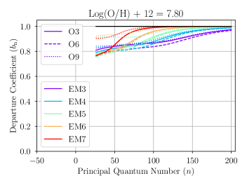
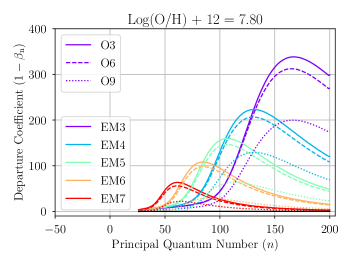
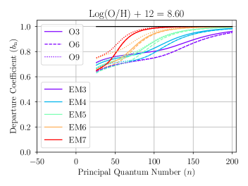
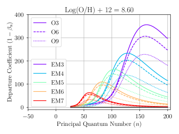
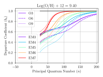
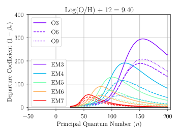
Figure 3: Departures from LTE in our CLOUDY simulations. Plotted are the departure coefficients $b_{\rm n}$ (left) and $\beta_{\rm n}$ (right) as a function of $n$. Different metallicities are shown with Log(O/H) + 12 values of 7.8 (top), 8.6 (middle), and 9.4 (bottom). The line color represents different emission measures, whereas the line style corresponds to different spectral types. The departure coefficients were taken from a representative numerical cell that has a depth 25% into the H ii region from the center of the model nebula. For cm-wavelength RRLs, $n\sim 100$.

The departure coefficient $b_{\rm n}$ is given by

$$b_{\rm n}=N_{\rm n}/N_{\rm n}^{*},$$ (3)

where $N_{\rm n}$ is the true population level and $N_{\rm n}^{*}$ is the population level in LTE for quantum level $n$. Since the Einstein $A$ coefficient for the lower state is larger and the atom is smaller so that collisions are less effective, $b_{\rm n}<1$. For $n=100$, $b_{\rm n}>0.8$ for most simulations but larger departures from LTE exist for the higher metallicities where the electron temperatures are smaller. Simulations with lower electron densities have larger departures from LTE since there are fewer collisions.

The departure coefficient $\beta_{\rm n}$ is a measure of the gradient of $b_{\rm n}$ with respect to $n$ and is given by (Wilson et al., 2009):

$$\beta_{\rm n}=1-20.836\Big{(}\frac{T_{\rm e}}{\rm K}\Big{)}\Big{(}\frac{\nu_{\rm L}}{\rm GHz}\Big{)}^{-1}\frac{{\rm d}\,{\rm ln}\,b_{\rm n}}{{\rm d}n}\Delta{n}.$$ (4)

The values of $\beta_{\rm n}$ can be much different than unity and for inverted populations, $\beta_{\rm n}<0$, maser amplification occurs. For our simulations we see values as high as $\beta_{\rm n}\sim-300$, but how this alters the RRL intensities will depend on the detailed radiative transfer and continuum opacity (e.g., see Wilson et al., 2009).

How do the departure coefficients affect the electron temperature? Following Wilson et al. (2009), we estimate the non-LTE RRL electron temperature as

$$T_{\rm e}=T_{\rm e}^{*}\,[b_{\rm n}(1-\frac{1}{2}\beta_{\rm n}\tau_{\rm c})]^{0.87},$$ (5)

where $\tau_{\rm c}$ is the free-free continuum opacity. Equation 5 is an approximation to a uniform region with a background opacity $\tau_{\rm c}$. In practice, the equation of transfer must be solved from the back of the nebula to the front with respect to the observer. If the nebula is optically thin, however, ($1-\frac{1}{2}\beta_{\rm n}\tau_{\rm c})\sim 1$ and so $T_{\rm e}\sim T_{\rm e}^{*}\,b_{\rm n}^{0.87}$. Because most nebulae are optically thin at cm-wavelengths, deviations from LTE will be mostly due to $b_{\rm n}$. Since $b_{\rm n}<1$, electron temperatures calculated assuming LTE will overestimate the true electron temperature.

Figure 4 compares the “real” electron temperature, $T_{\rm e}^{n_{\rm e}n_{\rm p}}$, to the “synthetic” electron temperature derived using RRLs assuming LTE, $T_{\rm e}^{*}$, for all 135 simulation. As expected, $T_{\rm e}^{*}>T_{\rm e}^{n_{\rm e}n_{\rm p}}$ for almost all simulations. Electron temperatures derived assuming LTE are about 20% systematically higher than the “real” electron temperature. For model nebula with low densities and high metallicities the difference can be as high as 50%. The plots on the right correct the electron temperatures for departures from LTE assuming an optically thin nebula and account for most, but not all, of the discrepancy.

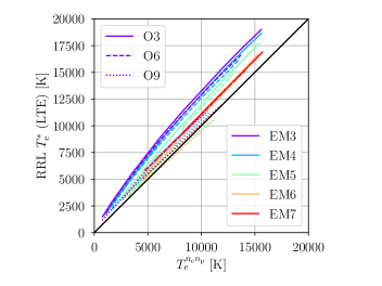
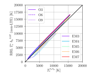
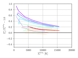
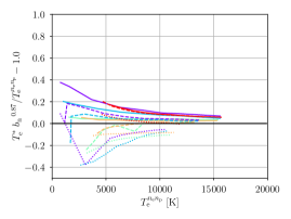
Figure 4: Accuracy of electron temperatures derived using RRLs. The electron temperature, $T_{\rm e}^{n_{\rm e}n_{\rm p}}$, is determined by averaging the $n_{\rm e}n_{\rm p}$-weighted electron temperatures over the volume of the model spherical nebula. The RRL-derived electron temperature is calculated from the synthetic H87$\alpha$ RRL and free-continuum emission produced by the CLOUDY simulation assuming LTE (left) and non-LTE (right). Here we assume the gas is optically thin so $T_{\rm e}=T_{\rm e}^{*}\,b_{\rm n}^{0.87}$ (Wilson et al., 2009). We plot the results of this comparison for all 135 simulations. The nine different metallicities provide the wide range of electron temperatures shown as curves in the plots. The line color represents different emission measures, whereas the line style corresponds to different spectral types. The bottom panels plot the fractional difference to reveal details.

3.2 CLOUDY Metallicity-Electron Temperature Relationship

There is an empirical correlation between the metallicity, probed by the O/H abundance ratio, and electron temperature because the metallicity is the main factor that regulates the temperature in H ii regions (e.g., Rubin, 1985). But the ionizing radiation field spectrum and the nebular density also influence the thermal properties of the H ii region. Figure 5 summarizes the metallicity-electron temperature relationship produced by the CLOUDY simulations. The left panel plots Log(O/H) + 12 as a function of the “real” electron temperature, $T_{\rm e}^{n_{\rm e}n_{\rm p}}$, for all 135 simulations. The line color represents different emission measures, whereas the line style corresponds to different spectral types. The black solid line is the empirical metallicity-electron temperature relationship determined by Shaver et al. (1983) and given by:

$${\rm Log(O/H)}+12=(9.82\pm 0.02)-(1.49\pm 0.11)T_{\rm e}/10^{4}.$$ (6)

This empirical relationship is consistent with the CLOUDY results but there is considerable scatter due to differences in the spectral type of the ionizing star and the nebular electron density. For example, simulations with earlier type stars or higher electron densities have higher electron temperatures. The right panel plots the same relationship using the “synthetic” electron temperature, $T_{\rm e}^{*}$. Here the scatter is larger with a systematic offset. This is primarily due to departures from LTE that can overestimate the electron temperature, especially for earlier type stars with lower emission measures (see Section 3.1).

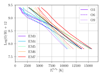
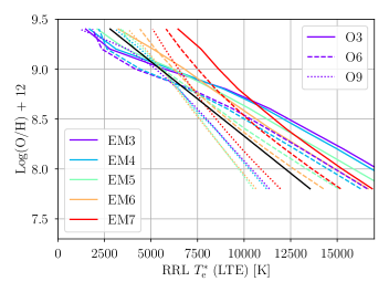
Figure 5: The oxygen abundance ratio, Log(O/H) + 12, as a function of electron temperature for all 135 CLOUDY simulations. Left: The electron temperature is determined by averaging the $n_{\rm e}n_{\rm p}$-weighted electron temperatures over the volume of the model spherical nebula. Right: The RRL-derived electron temperature calculated from the synthetic H87$\alpha$ RRL and free-continuum emission produced by the CLOUDY simulation assuming LTE. The line color represents different emission measures and the line style corresponds to different spectral-types. The black solid line is the metallicity-electron temperature relationship from Shaver et al. (1983). Generally, the electron temperature increases with earlier spectral-type stars and increasing electron density.

4 Discussion

To determine the Galactic metallicity structure from radio data requires RRL and free-free continuum observations in H ii regions and a metallicity-electron temperature relationship (e.g., Wenger et al., 2019). Here we show that non-LTE effects and variations in the physical properties of the ionized gas produce systematic errors in the Galactic metallicity structure. RRL and free-free continuum emission toward H ii regions provide an accurate measure of $T_{\rm e}$ if the nebula is optically thin and the ionized gas is in LTE. Studies have shown that at cm-wavelengths that these conditions are valid in many H ii regions (Shaver, 1980a, b). Pressure broadening via electron impacts can alter the line shape, causing an underestimate of the integrated RRL emission when the spectral baselines are not well behaved. This can especially be an issue for single-dish radio telescopes (e.g., see Balser et al., 1999), but is not a significant issue for radio interferometers (e.g., Balser et al., 2022). Stimulated emission is not common at cm-wavelengths and typically requires a bright background source with a specific geometry (e.g., Martin-Pintado et al., 1989).

Our CLOUDY simulations show, however, that non-LTE effects are important when attempting to derive accurate electron temperatures. In particular, electron temperatures are systematically higher by about 20% when assuming LTE, and in some cases are 50% larger for low density nebula (see Figure 4). Since we are mostly interested in metallicity structure (e.g., radial or azimuthal gradients), systematic offsets are less important than the dispersion in these offsets. Nevertheless, such uncertainties need to be included in any analysis of metallicity structure when using RRL and continuum data to derive electron temperatures. We therefore calculate correction factors for the electron temperature when LTE is assumed. Specifically, the correction factor is the ratio of the “real” electron temperature to the “synthetic” electron temperature, $T_{\rm e}^{n_{\rm e}n_{\rm p}}$/$T_{\rm e}^{*}$. The electron temperature correction factors are shown as contour plots in Figure 6 for spectral types O3, O6, and O9. The correction factors are typically less than unity for most simulations since the electron temperatures are systematically higher when assuming LTE. For nebulae ionized by O9 stars, however, the correction factors are closer to unity.

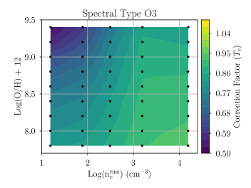
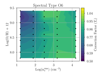
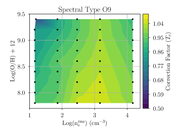
Figure 6: Correction factors of the electron temperature for ionizing stars with spectral-types O3, O6, and O9. The correction factor is the ratio of the “real” electron temperature to the “synthetic” electron temperature, $T_{\rm e}^{n_{\rm e}n_{\rm p}}$/$T_{\rm e}^{*}$. The black points correspond to the location, defined by Log(O/H) + 12 and $n_{\rm e}^{\rm rms}$ from each simulation, from which the contours are generated. The contour levels are between 0.5 and 1.1 with an increment of 0.03. For most simulations the predicted electron temperature is overestimated yielding correction factors less than unity.

The metallicity-electron relationship exists since heavy elements primarily regulate the thermal properties of the ionized gas. To determine the metallicity-electron temperature H ii region relationship requires the abundance of a heavy element (e.g., oxygen) relative to hydrogen. Many studies employ CELs at optical wavelengths since they are bright. To derive O/H directly, however, requires the electron temperature—the $T_{\rm e}$-method. Electron temperatures are often determined using the ratio of nebular lines to the higher energy level auroral lines; for example, [O iii]$\lambda\lambda$4959, 5007/$\lambda$4363 (e.g., Peimbert & Costero, 1969). Unfortunately, [O iii]$\lambda$4363 is weak and often not detected, so indirect methods have been developed. For example, Pagel et al. (1979) suggested the $R_{23}$-method, an empirical strong line method, which uses bright transitions to form the ratio ([O ii]$\lambda\lambda$3726, 3729 + [O iii]$\lambda\lambda$4959, 5007)/H$\beta$. Many other approaches or calibrations have been investigated (see Pilyugin & Grebel, 2016; Peimbert et al., 2017, and references within).

Shaver et al. (1983) employed a novel approach by using RRLs to determine the electron temperature instead of optical data and then applied these values of $T_{\rm e}$ to the empirical formulae to calculate the O/H abundance ratio. The Shaver et al. (1983) metallicity-electron temperature relationship therefore self-consistently uses the radio data. There have since been several studies, however, that produce different results. For example, Pilyugin et al. (2003) used the $T_{\rm e}$-method and found systematically lower O/H abundance ratios by 0.2–0.3 dex. The different results are due to different atomic data and different assumptions about the temperature structure. For recent studies with more sensitive observations and updated atomic data see Arellano-Córdova et al. (2020, 2021).

Temperature fluctuations within the nebula can produce different evaluations of $T_{\rm e}$ depending on the method and therefore different O/H abundance ratios (Peimbert, 1967). This is thought to be at least one explanation for the discrepancy between heavy element abundances derived from CELs and optical recombination lines (ORLs) that has existed for many years (Wyse, 1942). Méndez-Delgado et al. (2023) suggested that temperature fluctuations are confined to the central regions of a nebula, which primarily affects the highly ionized gas traced by [O iii], and causes the abundance discrepancy problem. They derived a new metallicity-electron temperature relationship, based on data from both Galactic and extragalacitc H ii regions, appropriate when $T_{\rm e}$ is determined using recombination lines and therefore appropriate for RRLs:

$${\rm Log(O/H)}+12=(9.44\pm 0.08)-(1.07\pm 0.09)T_{\rm e}/10^{4}.$$ (7)

The intercept of this linear relationship is similar to that of Shaver et al. (1983) but the slope is about 1.4 times smaller (see Figure 7). Shaver et al. (1983) estimated that temperature fluctuations in their H ii region sample were small, $t^{2}\lesssim 0.015$, based on values of $T_{\rm e}$ derived from RRLs and CELs. Here, $t^{2}$ is the root-mean-square (rms) deviation from the average electron temperature. In contrast, Méndez-Delgado et al. (2023) estimate $t^{2}>0.025$ for most of the H ii regions in their sample. The quality of the optical spectra and the accuracy of the atomic data are clearly very different between the two studies. Moreover, the sample by Méndez-Delgado et al. (2023) includes giant H ii regions with lower densities and metallicities. Therefore, a comparison between the two metallicity-electron temperature relationships may not be appropriate.

Another approach is to use CELs at far-infrared (FIR) wavelengths. They have several advantages over optical CELs: (1) there is less extinction from dust; and (2) they are not very sensitive to electron temperature and thus temperature fluctuations. But FIR CELs are sensitive to electron density and are less bright then their optical counterparts. Rudolph et al. (2006) reanalyzed observations from the literature (Simpson et al., 1995; Afflerbach et al., 1997; Rudolph et al., 1997; Peeters et al., 2002) in a self-consistent way to derive the O/H abundance ratio toward H ii regions in the Galactic disk using the FIR lines of [O iii] (52µm and 88µm). Their results are plotted in Figure 7 where the electron temperatures have been determined from RRLs (Wenger et al., 2019). The large uncertainties in the FIR-determined O/H abundance ratios cannot distinguish between the two metallicity-electron temperature relationships.

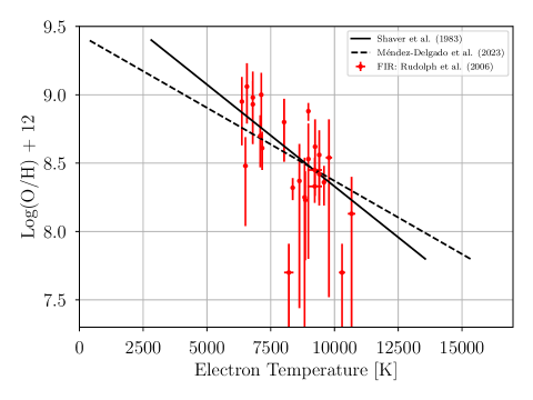
Figure 7: Metallicity-electron temperature H ii region relationships from Shaver et al. (1983) (solid line) and Méndez-Delgado et al. (2023) (dashed line). The red circles denote O/H abundance ratios from FIR CELs (Rudolph et al., 2006) and electron temperatures from RRLs (Wenger et al., 2019). Here, we exclude the results from Peeters et al. (2002) which yield systematically lower O/H abundance ratios.

Because other factors besides metallicity will affect the electron temperature, no single linear relationship will hold between O/H and $T_{\rm e}$. Moreover, most H ii regions in the Milky Way are not accessible to optical studies due to dust extinction (Anderson et al., 2014), and therefore the diagnostic tracers of various nebular properties (e.g., $t^{2}$) are not available. Here, we therefore use the CLODUY simulations to assess the uncertainties in the metallicity-electron temperature relationship and provide correction factors to Log(O/H) + 12 when using radio data. Specifically, the correction factor is the ratio of Log(O/H) + 12 input into the CLOUDY simulation to the Log(O/H) + 12 value derived from the Shaver et al. metallicity-electron temperature relationship using the LTE electron temperature calculated from the synthetic H87$\alpha$ RRL in the CLOUDY simulation. The fractional uncertainty is just the correction factor minus 1.0.

The results are summarized as contour plots in Figure 8 for spectral types O3, O6, and O9. The correction factors depend on the O/H abundance ratios input into the CLOUDY simulation and the electron density. Here we derive a rms electron density in the same way as would be done using radio observations: $n_{\rm e}^{\rm rms}=\sqrt{EM/D}$. For the CLOUDY simulations we calculate the emission measure as $EM=\sum_{\rm i=1}^{\rm N}n_{\rm e,i}^{2}\Delta\ell_{\rm i}$, where $n_{\rm e,i}$ is the electron density in numerical zone i, $\Delta\ell_{\rm i}$ is the width of zone i, and N is the number of zones.

Table 2 summarizes the correction factors for both the electron temperature and O/H abundance ratio. Listed are the spectral type of the ionizing star, the rms electron density, the metallicity given by Log(O/H) + 12, and the correction factors. The correction factors are a measure of the uncertainty when using radio tracers to determine metallicity, but in principle they may also be used to correct for systematic uncertainties if the spectral type, electron density, and metallicity can be estimated (e.g., Schraml & Mezger, 1969). This is an iterative process because the correction factor is a function of metallicity. Overall, the correction factors are less than 10% from unity. For lower metallicities the correction factor depends on the spectral-type of the ionizing star, whereas for higher metallicities the correction factor is sensitive to the electron density.

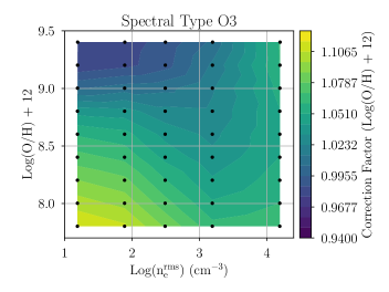
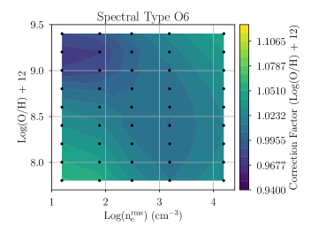
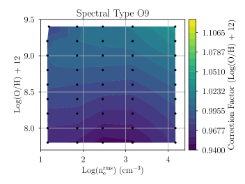
Figure 8: Correction factors of Log(O/H) + 12 for ionizing stars with spectral-types O3, O6, and O9. The correction factor is the ratio of the O/H abundance input into the CLOUDY simulation to the O/H abundance derived from the Shaver et al. (1983) metallicity-electron temperature relationship using the LTE electron temperature calculated from the synthetic H87$\alpha$ RRL in the CLOUDY simulation. The black points correspond to the location, defined by Log(O/H) + 12 and $n_{\rm e}^{\rm rms}$ from each simulation, from which the contours are generated. The contour levels are between 0.94 and 1.125 with an increment of 0.00925. For lower metallicities the correction factor depends on the spectral-type of the ionizing star, whereas for higher metallicities the correction factor is sensitive to the electron density.

5 Summary

Heavy element abundances, or the metallicity, in H ii regions provide important constraints to Galactic chemical evolution models. Radio recombination lines from H ii regions are one of the few tracers that are not affected by dust and therefore probe the entire Galactic disk. RRL emission from elements heavier than helium, however, is too weak to be detected in H ii regions. Since metals act as coolants they primarily regulate the thermal motions of the ionized gas to produce a linear relationship between metallicity and electron temperature. Assuming LTE, the ratio of the RRL to the radio free-free continuum provides a measure of the electron temperature independent from the electron density, and therefore a way to indirectly determine the metallicity (Wenger et al., 2019).

Here, we use CLOUDY simulations to investigate the uncertainties in this indirect method of determining the metallicity from radio data. We run 135 CLOUDY simulations varying the spectral type, electron density, and metallicity (defined by the O/H abundance ratio). We find that electron temperatures derived assuming LTE are about 20% higher, but overall LTE is a good assumption for cm-wavelength RRLs. Overall, the CLOUDY simulation results are consistent with the metallicity-electron temperature relationship determined empirically by Shaver et al. (1983). But there exists significant dispersion since ionizing stars with earlier spectral types or nebulae with higher electron density yield higher electron temperatures. When combined the errors in the predicted metallicity, defined by Log(O/H) + 12, are less than 10%. We derive correction factors to the Shaver et al. (1983) metallicity-electron temperature relationship that depend on the spectral type, electron density, and metallicity.

Table 2: Correction Factor

Spectral	Log($n_{\rm e}^{\rm rms}$)	Log(O/H) + 12	Correction Factor
Type	(cm-3)		$T_{\rm e}$	Log(O/H) + 12
O3	1.191	8.4	0.7564	1.0730
O3	1.890	8.4	0.7741	1.0668
O3	2.492	8.4	0.8338	1.0483
O3	3.191	8.4	0.9021	1.0349
O3	4.191	8.4	0.9056	1.0511
O3	1.191	8.2	0.7769	1.0882
O3	1.890	8.2	0.7941	1.0811
O3	2.492	8.2	0.8423	1.0607
O3	3.191	8.2	0.9058	1.0432
O3	4.191	8.2	0.9178	1.0550
O3	1.191	8.0	0.7980	1.1019
O3	1.890	8.0	0.8143	1.0942
O3	2.492	8.0	0.8576	1.0731
O3	3.191	8.0	0.9146	1.0523
O3	4.191	8.0	0.9243	1.0603
O3	1.191	7.8	0.8211	1.1163
O3	1.890	7.8	0.8361	1.1083
O3	2.492	7.8	0.8689	1.0868
O3	3.191	7.8	0.9182	1.0633
O3	4.191	7.8	0.9301	1.0681
O3	1.191	8.6	0.7272	1.0592
O3	1.890	8.6	0.7535	1.0543
O3	2.492	8.6	0.8161	1.0386
O3	3.191	8.6	0.8937	1.0300
O3	4.191	8.6	0.8986	1.0505
O3	1.191	8.8	0.6927	1.0383
O3	1.890	8.8	0.7262	1.0362
O3	2.492	8.8	0.8012	1.0262
O3	3.191	8.8	0.8861	1.0250
O3	4.191	8.8	0.8868	1.0506
O3	1.192	9.0	0.6405	1.0037
O3	1.891	9.0	0.6906	1.0094
O3	2.493	9.0	0.7867	1.0113
O3	3.192	9.0	0.8769	1.0221
O3	4.192	9.0	0.8728	1.0548
O3	1.193	9.2	0.5700	0.9785
O3	1.892	9.2	0.6454	0.9836
O3	2.494	9.2	0.7694	0.9916
O3	3.193	9.2	0.8687	1.0157
O3	4.193	9.2	0.8551	1.0607
O3	1.195	9.4	0.5199	0.9796
O3	1.894	9.4	0.6074	0.9827
O3	2.496	9.4	0.7430	0.9892
O3	3.195	9.4	0.8441	1.0070
O3	4.195	9.4	0.8309	1.0613
O6	1.190	8.4	0.7520	1.0320
O6	1.889	8.4	0.7760	1.0252
O6	2.491	8.4	0.8419	1.0095
O6	3.190	8.4	0.9118	1.0042
O6	4.190	8.4	0.9023	1.0232
O6	1.190	8.2	0.7791	1.0423
O6	1.889	8.2	0.7944	1.0349
O6	2.491	8.2	0.8536	1.0152
O6	3.190	8.2	0.9147	1.0054
O6	4.190	8.2	0.9112	1.0246
O6	1.190	8.0	0.8008	1.0521
O6	1.889	8.0	0.8216	1.0444
O6	2.491	8.0	0.8686	1.0219
O6	3.190	8.0	0.9245	1.0085
O6	4.190	8.0	0.9169	1.0274
O6	1.190	7.8	0.8246	1.0623
O6	1.889	7.8	0.8365	1.0547
O6	2.491	7.8	0.8754	1.0302
O6	3.190	7.8	0.9256	1.0139
O6	4.190	7.8	0.9285	1.0324
O6	1.191	8.6	0.7228	1.0218
O6	1.890	8.6	0.7533	1.0164
O6	2.484	8.6	0.8922	1.0074
O6	3.189	8.6	0.9130	1.0049
O6	4.191	8.6	0.8921	1.0253
O6	1.191	8.8	0.6844	1.0051
O6	1.890	8.8	0.7234	1.0028
O6	2.492	8.8	0.8246	1.0049
O6	3.187	8.8	0.9178	1.0074
O6	4.191	8.8	0.8777	1.0284
O6	1.191	9.0	0.6291	0.9783
O6	1.890	9.0	0.6843	0.9823
O6	2.489	9.0	0.8460	1.0021
O6	3.186	9.0	0.9209	1.0121
O6	4.192	9.0	0.8607	1.0345
O6	1.192	9.2	0.5905	0.9718
O6	1.891	9.2	0.6746	0.9762
O6	2.486	9.2	0.9289	0.9998
O6	3.184	9.2	0.9309	1.0179
O6	4.193	9.2	0.8403	1.0414
O6	1.193	9.4	0.6196	0.9852
O6	1.892	9.4	0.7724	0.9905
O6	2.484	9.4	0.9406	1.0090
O6	3.182	9.4	0.9493	1.0260
O6	4.194	9.4	0.8089	1.0500
O9	1.164	8.4	0.8744	0.9817
O9	1.860	8.4	0.9352	0.9812
O9	2.461	8.4	1.0045	0.9749
O9	3.163	8.4	1.0401	0.9740
O9	4.171	8.4	0.9719	0.9897
O9	1.164	8.2	0.8933	0.9744
O9	1.861	8.2	0.9393	0.9733
O9	2.461	8.2	1.0218	0.9653
O9	3.163	8.2	1.0482	0.9652
O9	4.171	8.2	0.9804	0.9824
O9	1.165	8.0	0.9111	0.9673
O9	1.862	8.0	0.9481	0.9653
O9	2.460	8.0	1.0313	0.9554
O9	3.163	8.0	1.0554	0.9565
O9	4.172	8.0	0.9833	0.9760
O9	1.165	7.8	0.9337	0.9598
O9	1.862	7.8	0.9549	0.9573
O9	2.460	7.8	1.0489	0.9449
O9	3.162	7.8	1.0625	0.9474
O9	4.172	7.8	0.9962	0.9704
O9	1.163	8.6	0.8564	0.9882
O9	1.857	8.6	0.9491	0.9860
O9	2.461	8.6	0.9888	0.9843
O9	3.163	8.6	1.0329	0.9830
O9	4.170	8.6	0.9611	0.9979
O9	1.163	8.8	0.8376	0.9935
O9	1.857	8.8	0.9241	0.9947
O9	2.461	8.8	0.9718	0.9934
O9	3.163	8.8	1.0251	0.9923
O9	4.170	8.8	0.9502	1.0070
O9	1.161	9.0	0.8298	0.9961
O9	1.858	9.0	0.8973	1.0014
O9	2.462	9.0	0.9553	1.0015
O9	3.164	9.0	1.0177	1.0012
O9	4.169	9.0	0.9362	1.0166
O9	1.156	9.2	0.8259	0.9933
O9	1.858	9.2	0.8704	1.0045
O9	2.462	9.2	0.9402	1.0073
O9	3.164	9.2	1.0120	1.0093
O9	4.169	9.2	0.9196	1.0267
O9	1.194	9.4	0.6392	0.9747
O9	1.859	9.4	0.8566	1.0042
O9	2.463	9.4	0.9404	1.0096
O9	3.165	9.4	1.0103	1.0154
O9	4.168	9.4	0.9023	1.0375

Appendix A CLOUDY Simulation Parameters

Below are the inputs for one CLOUDY simulation that consisted of a O6-type ionizing star and a model nebula with $n_{\rm H}=200$$\,{\rm cm^{-3}}$, $D=2.5$$\,{\rm pc}$, and ${\rm Log(O/H)}+12=8.8$.

title hii_O6_em5_m0.2_starz
# commands controlling continuum =========
table star atlas Z-1.5 38151.0
q(h) 48.96
# commands controlling geometry  =========
sphere
radius 0.001 to 1.25 linear parsecs
# commands for density & abundances =========
hden 200.0 linear
abundances "HII.abn" no grains
metals 0.2 log
filling 1.
# number of levels to use
database h-like resolved levels 25
database h-like collapsed levels 375
database he-like resolved levels 20
database he-like collapsed levels 380
# collisional excitation data (default is lebedev)
#database h-like collisions lebedev
# other commands for details     =========
iterate
# Allow for lower temperatures (default is Te=4000K)
stop temperature 1000.0 linear
# commands controlling output    =========
# set continuum frequencies
set nFnu add 3.00299 cm
set nFnu add 3.05299 cm
set nFnu add 3.10299 cm
set nFnu add 3.15887 cm
set nFnu add 3.20887 cm
set nFnu add 3.26716 cm
set nFnu add 3.31716 cm
set nFnu add 3.37791 cm
set nFnu add 3.42791 cm
set nFnu add 3.49113 cm
set nFnu add 3.54113 cm
set nFnu add 3.60686 cm
set nFnu add 3.65686 cm
set nFnu add 3.72511 cm
set nFnu add 3.77511 cm
# save details about calculation and model
save performance "hii_O6_em5_m0.2_starz.per"
save overview last "hii_O6_em5_m0.2_starz.ovr"
save dr last "hii_O6_em5_m0.2_starz.dr"
save incident continuum last "hii_O6_em5_m0.2_starz.inc"
save continuum last "hii_O6_em5_m0.2_starz.con" units microns
save transmitted continuum last "hii_O6_em5_m0.2_starz.trn"
save line list "hii_O6_em5_m0.2_starz.linaC" "linelistOnlyCont.dat" last absolute
save line list "hii_O6_em5_m0.2_starz.lineaL" "linelistNoCont.dat" last emergent absolute
save hydrogen lines alpha last "hii_O6_em5_m0.2_starz.hlin"
save species departure coefficients last "hii_O6_em5_m0.2_starz.dep" "H[:]"
# hii_O6_em5_m0.2_starz.in

References

- Afflerbach et al. (1997) Afflerbach, A., Churchwell, E., & Werner, M. W. 1997, ApJ, 478, 190, doi: 10.1086/303771
- Anderson et al. (2014) Anderson, L. D., Bania, T. M., Balser, D. S., et al. 2014, ApJS, 212, 1, doi: 10.1088/0067-0049/212/1/1
- Anderson et al. (2011) Anderson, L. D., Bania, T. M., Balser, D. S., & Rood, R. T. 2011, ApJS, 194, 32, doi: 10.1088/0067-0049/194/2/32
- Arellano-Córdova et al. (2020) Arellano-Córdova, K. Z., Esteban, C., García-Rojas, J., & Méndez-Delgado, J. E. 2020, MNRAS, 496, 1051, doi: 10.1093/mnras/staa1523
- Arellano-Córdova et al. (2021) —. 2021, MNRAS, 502, 225, doi: 10.1093/mnras/staa3903
- Baldwin et al. (1991) Baldwin, J. A., Ferland, G. J., Martin, P. G., et al. 1991, ApJ, 374, 580, doi: 10.1086/170146
- Balser et al. (1999) Balser, D. S., Bania, T. M., Rood, R. T., & Wilson, T. L. 1999, ApJ, 510, 759, doi: 10.1086/306598
- Balser et al. (2011) Balser, D. S., Rood, R. T., Bania, T. M., & Anderson, L. D. 2011, ApJ, 738, 27, doi: 10.1088/0004-637X/738/1/27
- Balser et al. (2015) Balser, D. S., Wenger, T. V., Anderson, L. D., & Bania, T. M. 2015, ApJ, 806, 199, doi: 10.1088/0004-637X/806/2/199
- Balser et al. (2022) Balser, D. S., Wenger, T. V., & Bania, T. M. 2022, ApJ, 936, 168, doi: 10.3847/1538-4357/ac87a6
- Bania et al. (2007) Bania, T. M., Balser, D. S., Rood, R. T., Wilson, T. L., & LaRocque, J. M. 2007, ApJ, 664, 915, doi: 10.1086/519453
- Brocklehurst & Seaton (1972) Brocklehurst, M., & Seaton, M. J. 1972, MNRAS, 157, 179, doi: 10.1093/mnras/157.2.179
- Caplan et al. (2000) Caplan, J., Deharveng, L., Peña, M., Costero, R., & Blondel, C. 2000, MNRAS, 311, 317, doi: 10.1046/j.1365-8711.2000.03029.x
- Castelli & Kurucz (2003) Castelli, F., & Kurucz, R. L. 2003, in Modelling of Stellar Atmospheres, ed. N. Piskunov, W. W. Weiss, & D. F. Gray, Vol. 210, A20, doi: 10.48550/arXiv.astro-ph/0405087
- Chatzikos et al. (2023) Chatzikos, M., Bianchi, S., Camilloni, F., et al. 2023, arXiv e-prints, arXiv:2308.06396, doi: 10.48550/arXiv.2308.06396
- Chiappini et al. (2001) Chiappini, C., Matteucci, F., & Romano, D. 2001, ApJ, 554, 1044, doi: 10.1086/321427