Avoiding breakdown in incomplete factorizations in low precision arithmetic

Abstract

The emergence of low precision floating-point arithmetic in computer hardware has led to a resurgence of interest in the use of mixed precision numerical linear algebra. For linear systems of equations, there has been renewed enthusiasm for mixed precision variants of iterative refinement. We consider the iterative solution of large sparse systems using incomplete factorization preconditioners. The focus is on the robust computation of such preconditioners in half precision arithmetic and employing them to solve symmetric positive definite systems to higher precision accuracy; however, the proposed ideas can be applied more generally. Even for well-conditioned problems, incomplete factorizations can break down when small entries occur on the diagonal during the factorization. When using half precision arithmetic, overflows are an additional possible source of breakdown. We examine how breakdowns can be avoided and we implement our strategies within new half precision Fortran sparse incomplete Cholesky factorization software. Results are reported for a range of problems from practical applications. These demonstrate that, even for highly ill-conditioned problems, half precision preconditioners can potentially replace double precision preconditioners, although unsurprisingly this may be at the cost of additional iterations of a Krylov solver.

1 Introduction

We are interested in solving sparse linear systems $Ax=b$, where $A\in\mathbb{R}^{n\times n}$ is nonsingular and $x,b\in\mathbb{R}^{n}$. The majority of algorithms for solving such systems fall into two main categories: direct methods and iterative methods. Direct methods transform $A$ using a finite sequence of elementary transformations into a product of simpler sparse matrices in such a way that solving linear systems of equations with the factor matrices is comparatively easy and inexpensive. For example, for a general nonsymmetric matrix, $A=PLUQ$, where $L$ is a lower triangular matrix, $U$ is an upper triangular matrix, and $P$ and $Q$ are permutation matrices chosen to preserve sparsity in the factors and ensure the factorization is stable. Direct methods, when properly implemented, are robust and can be confidently used as black-box solvers for computing solutions with predictable accuracy, which is typically at the level of double precision. However, they require significant expertise to implement efficiently (particularly in parallel). They also need large amounts of memory (which increases nonlinearly with the size and density of $A$) and the matrix factors normally contain many more nonzero entries than $A$; these extra entries are termed the fill-in and much effort goes into trying to minimise the amount of fill-in.

By contrast, iterative methods compute a sequence of approximations ${x}^{(0)},{x}^{(1)},{x}^{(2)},\ldots$ that (hopefully) converge to the solution in an acceptable number of iterations. The number of iterations (and whether or not convergence occurs at all) depends on ${x}^{(0)}$, $A$ and $b$ as well as the required accuracy in $x$. Basic implementations of iterative solvers are relatively straightforward as they only use the sparse matrix $A$ indirectly, through matrix-vector products and, most importantly, their memory demands are limited to a (small) number of vectors of length $n$, making them attractive for very large problems and problems where $A$ is not available explicitly. However, preconditioning is usually essential to enhance convergence of the iterative method. Preconditioning seeks to transform the system into one that is more tractable and from which the required solution of the original system can easily be recovered. Determining and computing effective preconditioners is highly problem dependent and generally very challenging. Algebraic preconditioners that are built using an incomplete factorization of $A$ in which entries that would be part of a complete factorization are dropped are frequently used, especially when the underlying physics of the problem is difficult to exploit. Such preconditioners can be employed within more sophisticated methods; for example, to precondition subdomain solves in domain decomposition schemes or as smoothers in multigrid methods.

The performance differences for computing and communicating in different precision formats has led to a long history of efforts to enhance numerical algorithms by combining precision formats. The goals of mixed-precision algorithms include accelerating the computational time by including the use of lower-precision formats while obtaining high-precision accuracy of the output and, by reducing the memory requirements, extending the size of problems that can be solved as well as potentially lowering energy usage. Numerical linear algebra software, and linear system solvers in particular, traditionally use double precision (64-bit) arithmetic, although some packages (including the BLAS and LAPACK routines and some sparse solvers, such as those in the HSL mathematical software library [HSL(2023)]) have always also offered single precision (32-bit) versions. In the mid 2000s, the speed difference between single and double precision arithmetic on what were then state-of-the-art architectures, notably Sony/Toshiba/IBM Cell processors (see, for example, [Buttari et al.(2007a), Kurzak and Dongarra(2007), Langou et al.(2006)]), led to studies into the feasibility of factorizing a matrix in single precision and then using the factors as a preconditioner for a simple iterative method to regain higher precision accuracy [Arioli and Duff(2009), Buttari et al.(2008), Buttari et al.(2007b)]. Hogg and Scott [Hogg and Scott(2010)] extended this to develop a mixed precision sparse symmetric indefinite solver. More recently, the potential for employing single precision arithmetic in solving sparse systems to double precision accuracy using multiple cores has been considered by Zounon et al [Zounon et al.(2022)]. For such systems, the integer data used to hold the sparse structures of the matrix and its factors is independent of the precision and memory savings come only from the real factor data. However, this does have the potential to increase the size of problem that can be tackled and, in the incomplete factorization case, to allow more entries to be retained in the factors, which can result in a higher quality preconditioner, leading to savings in the total solution time.

In the past few years, the emergence of lower precision arithmetic in hardware has led to further interest in mixed precision algorithms. A key difference compared to earlier work is the use of half precision (16-bit) arithmetic. A comprehensive state-of-the-art survey of work on mixed precision numerical linear algebra routines (including an extensive bibliography) is given in [Higham and Mary(2022)] (see also [Abdelfattah et al.(2021)]). In particular, there have been important ideas and theory on mixed precision iterative refinement methods that employ the matrix factors computed in low precision as a preconditioner to recover higher precision accuracy [Amestoy et al.(2021), Carson and Higham(2017), Carson and Higham(2018)]. The number of entries in the factors of a sparse matrix $A$ is typically much greater than in $A$ and so, unlike in the dense case, the overhead of keeping a high precision copy of $A$ for computing the residual in the refinement process is small. Amestoy et al [Amestoy et al.(2023)] investigate the potential of mixed precision iterative refinement to enhance methods for sparse systems based on a particular class of approximate sparse factorizations. They employ the well-known parallel sparse direct solver MUMPS [Amestoy et al.(2000)], which is able to exploit block low-rank factorizations and static pivoting to compute approximate factors. The reported results in [Amestoy et al.(2023)] are restricted to combining single and double precision arithmetic because, in common with all other currently available sparse direct solvers, MUMPS does not yet support the use of half precision arithmetic. Developing an efficient half precision solver is not straightforward, requiring 16-bit versions of the dense linear algebra routines that provide the building blocks behind direct solvers. Such routines are now becoming available (for example, dense matrix-matrix multiplication in half precision is now supported by NVIDIA’s cuBLAS library), making the future development of efficient software potentially more feasible.

Higham and Pranesh [Higham and Pranesh(2021)] focus on symmetric positive definite linear systems. They compute a Cholesky factorization using low precision arithmetic and employ the factors as preconditioners in GMRES-based and CG-based iterative refinement. While they are interested in the sparse case, their MATLAB experiments (which simulate low precision using their chop function [Higham and Pranesh(2019)]) store the sparse test examples as dense matrices and their Cholesky factorizations are computed using dense routines. The reported theoretical and numerical results demonstrate the potential for low precision (complete) factors to be used to obtain high precision accuracy. Most recently, Carson and Khan [Carson and Khan(2023)] have considered using sparse approximate inverse preconditioners (SPAI) that are based on Frobenius norm minimization [Grote and Huckle(1997)]. They again propose computing the preconditioner using low precision and then employing GMRES-based iterative refinement and report MATLAB experiments using the chop function. Mixed precision has also been investigated for multigrid methods (see, for example, the error analysis of McCormick et al [McCormick et al.(2021)], who observed that different levels in the grid hierarchy should use different precisions).

Our emphasis is on low precision incomplete factorization preconditioners, combined with Krylov subspace based iterative refinement. Although our ideas can be used for general sparse linear systems, we focus on the sparse symmetric positive definite case. We use half precision arithmetic to construct incomplete Cholesky factorizations that are then employed as preconditioners to recover double precision accuracy. Our primary objective is to show that for a range of problems (some of which are highly ill-conditioned) it is possible to successfully obtain and use low precision incomplete factors. We consider the potential sources of overflow during the incomplete factorization and look at how to safely detect and prevent overflow. We follow a number of others working on the development of numerical linear algebra algorithms in mixed precision in performing experiments that aim to explore the feasibility of the ideas by simulating half precision (see, for example, [Higham and Pranesh(2019), Carson et al.(2020), Carson and Khan(2023)]). We want the option to experiment with sparse problems that may be too large for MATLAB and have chosen to develop our software in Fortran. Half precision and double precision versions are tested on systems coming from practical applications.

This paper makes the following contributions:

(a) it considers the practicalities of computing classical incomplete factorizations using low precision arithmetic, in particular, the safe prediction of possible overflows;

(b) it successfully employs global modifications combined with a simple prescaling to prevent breakdowns during the factorization;

(c) it develops level-based incomplete Cholesky factorization software in half precision (written in Fortran);

(d) it demonstrates the potential for robust half precision incomplete factorization preconditioners to be used to solve ill-conditioned symmetric positive definite systems.

The rest of the paper is organised as follows. In Section 2, we briefly recall incomplete factorizations of sparse matrices and consider the challenges that incomplete Cholesky factorizations can face, particularly when low precision arithmetic is employed. In Section 3, we summarise basic mixed precision iterative refinement algorithms before presenting numerical results for a range of problems coming from practical applications in Section 4. Concluding remarks and possible future directions are given in Section 5.

Terminology. We use the term high precision for precision formats that provide high accuracy at the cost of a larger memory volume (in terms of bits) and low precision to refer to precision formats that compose of fewer bits (smaller memory volume) and provide low(er) accuracy. Unless stated otherwise, we mean IEEE double precision (64-bit) when using the term high precision (denoted by fp64) and the 1985 IEEE standard 754 half precision (16-bit) when using the term low precision (denoted by fp16). bfloat16 is another form of half-precision arithmetic that was introduced by Google in its tensor processing units and formalized by Intel; we do not use it in this paper. Table 1.1 summarises the parameters for different precision arithmetic. We use $u_{16}$ , $u_{32}$ , $u_{64}$ to denote the unit roundoffs in fp16, fp32, and fp64 arithmetic, respectively.

Table 1.1: Parameters for bfloat16, fp16, fp32, and fp64 arithmetic: the number of bits in the significand and exponent, unit roundoff $u$, smallest positive (subnormal) number $x^{s}_{min}$ , smallest normalized positive number $x_{min}$, and largest finite number $x_{max}$, all given to three significant figures. ${\dagger}$ In Intel’s bfloat16 specification, subnormal numbers are not supported.

	Signif.	Exp.	$\;\;u$	$\;x^{s}_{min}$	$\;x_{min}$	$\;x_{max}$
bfloat16	8	8	$3.91\times 10^{-3}$	$\;\;\;\dagger$	$1.18\times 10^{-38}$	$3.39\times 10^{38}$
fp16	11	5	$4.88\times 10^{-4}$	$5.96\times 10^{-8}$	$6.10\times 10^{-5}$	$6.55\times 10^{4}$
fp32	24	8	$5.96\times 10^{-8}$	$1.40\times 10^{-45}$	$1.18\times 10^{-38}$	$3.40\times 10^{38}$
fp64	53	11	$1.11\times 10^{-16}$	$4.94\times 10^{-324}$	$2.22\times 10^{-308}$	$1.80\times 10^{308}$

2 Incomplete factorizations

In this section, we briefly recall incomplete factorizations of sparse matrices and then discuss how breakdown can happen, particularly when using low precision.

2.1 A brief introduction to incomplete factorizations

For a general sparse matrix $A$, the incomplete factorizations that we are interested in are of the form $A\approx LU$, where $L$ and $U$ are sparse lower and upper triangular matrices, respectively (for simplicity of notation, the permutations $P$ and $Q$ that are for preserving sparsity in the factors are omitted). The computed incomplete factors are used to define the preconditioner; the preconditioned linear system is $U^{-1}L^{-1}A=U^{-1}L^{-1}b$. If $A$ is a symmetric positive definite (SPD) matrix then $A=LL^{T}$. There are three main classes of incomplete factorization preconditioners. Firstly, threshold-based $ILU(\tau)$ methods in which the locations of permissible fill-in in the factors are determined in conjunction with the numerical factorization of $A$; entries of the computed factors that are smaller than a prescribed threshold are dropped. Secondly, memory-based $ILU(m)$ methods in which the amount of memory available for the incomplete factorization is prescribed and only the largest entries are retained at each stage of the factorization. Thirdly, structure-based $ILU(\ell)$ methods in which an initial symbolic phase determines the location of permissible entries using only the sparsity pattern of $A$. The memory requirements for the incomplete factors are then determined before the numerical factorization is performed. The simplest such approach (for which the symbolic phase is trivial) is an $ILU(0)$ factorization (or $IC(0)$ in the SPD case) that limits entries in the incomplete factors to positions corresponding to entries in $A$ (no fill-in is permitted). $ILU(0)$ preconditioners are frequently used for comparison purposes when assessing the performance of other approaches.

The different approaches have been developed, modified and refined over many years. Variants have been proposed that combine the ideas and/or employ them in conjunction with discarding entries in $A$ (sparsification) before the factorization commences. For an introduction to ILU-based preconditioners and details of possible variants, we recommend [Chan and van der Vorst(1997)] and Chapter 10 of the book [Saad(2003)] and the references therein.

Algorithm 2.1 outlines a basic (right-looking) incomplete Cholesky (IC) factorization of a SPD matrix $A=\{a_{ij}\}$. Here all computations are performed in the same precision as $A$. The algorithm assumes a target sparsity pattern ${\mathcal{S}}\{L\}$ for $L=\{l_{ij}\}$ is provided, where

$${\mathcal{S}}\{L\}=\{(i,j)\,|\ l_{ij}\neq 0,\,1\leq j\leq i\leq n\}.$$

It is assumed that ${\mathcal{S}}\{L\}$ includes the diagonal entries. Modifications can be made to incorporate threshold dropping strategies and to determine ${\mathcal{S}}\{L\}$ as the method proceeds. At each major step $k$, outer product updates are applied to the part of the matrix that has not yet been factored (Lines 7–11).

 

Algorithm 2.1.

Basic right-looking IC factorization
Input: SPD matrix $A$ and a target sparsity pattern ${\mathcal{S}}\{L\}$
Output: Incomplete Cholesky factorization $A\approx LL^{T}$.  

1:Initialize $l_{ij}=a_{ij}$ for all $(i,j)\in{\mathcal{S}}\{L\}$

2:for $k=1:n$ do$\triangleright$ Start of $k$-th major step

3:     $l_{kk}\leftarrow(l_{kk})^{1/2}$$\triangleright$ Diagonal entry is the pivot

4:     for $i=k+1:n$ such that $(i,j)\in{\mathcal{S}}\{L\}$ do

5:         $l_{ik}\leftarrow l_{ik}/l_{kk}$ $\triangleright$ Scale pivot column $k$ of the incomplete factor by the pivot

6:     end for$\triangleright$ Column $k$ of $L$ has been computed

7:     for $j=k+1:n$ such that $(j,k)\in{\mathcal{S}}\{L\}$ do

8:         for $i=j:n$ such that $(i,j)\in{\mathcal{S}}\{L\}$  do

9:              $l_{ij}\leftarrow l_{ij}-l_{ik}l_{jk}$ $\triangleright$ Update operation on column $j$

10:         end for

11:     end for

12:end for

 

2.2 Breakdown during incomplete factorizations

For arbitrary choices of the sparsity pattern ${\mathcal{S}}\{L\}$, the incomplete Cholesky factorization exists if $A$ is an M-matrix or a H-matrix with positive diagonal entries [Meijerink and van der Vorst(1977), Manteuffel(1980)]. But for a general SPD matrix, there is no such guarantee and an incomplete factorization algorithm can (and frequently does) break down. There are three places where breakdown can occur. We refer to these as problems B1, B2, and B3 as follows.

• B1: The computed diagonal entry $l_{kk}$ (which is termed the pivot at step $k$) may be unacceptably small or negative.

• B2: The scaling $l_{ik}\leftarrow l_{ik}/l_{kk}$ may overflow.

• B3: The update $l_{ij}\leftarrow l_{ij}-l_{ik}l_{jk}$ may overflow.

It is crucial for a robust implementation to detect the possibility of overflow before it occurs (otherwise, the code will simply crash). Tests for potential breakdown must themselves only use operations that cannot overflow. We say that an operation is safe in the precision being used if it cannot overflow; otherwise it is unsafe.

Safe detection of problem B1 is straightforward as we simply need to check at Line 3 of Algorithm 2.1 that the pivot satisfies $l_{kk}\geq\tau>x_{min}$, where the threshold parameter $\tau$ depends on the precision used. Based on our experience with practical problems, in our reported results in Section 4, we use $\tau=10^{-5}$ for half precision factorizations and, for double precision factorizations, $\tau=10^{-20}$ (note that preconditioner quality is not sensitive to the precise choice of $\tau$).

Problem B2 can happen during the column scaling at Line 5 of Algorithm 2.1. Let $a$ be the entry of largest absolute value in the current pivot column $k$ and let $d$ denote the current pivot $l_{kk}$ (set at Line 3). If $a\leq x_{max}$ and $1\leq d\leq x_{max}$ then $d\geq a/x_{max}$ and it is safe to compute $a/d$ (and thus safe to scale column $k$).

Problem B3 can occur during the update operations at Line 9 of Algorithm 2.1. Algorithm 2.2 can be used to perform safe updates. Here the scalars and the computation are in the working precision.  

Algorithm 2.2.

Safe test for a safe update operation (detecting B3 breakdown)
Input: Scalars $a,b,c$ such that $|a|,|b|,|c|\leq x_{max}$.
Output: Either $v=a-bc$ or $flag=-3$ (unsafe to perform update).  

1:$flag=0$

2:if $|b|\leq 1$ or $|c|\leq 1$ then $\triangleright$ $x_{max}/|c|$ cannot be tested if $|c|<1$

3:     $w=bc$

4:else if $|b|\ \leq\ x_{max}/|c|$ then

5:     $w=bc$

6:else

7:     $flag=-3$ and return $\triangleright$ Unsafe to compute $bc$

8:end if

9:if $a\geq 0$  then

10:     if $w\geq 0$ or ($x_{max}-a\geq-w$) then

11:         $v=a-w$

12:     else

13:         $flag=-3$ and return $\triangleright$ Unsafe to perform subtraction

14:     end if

15:else

16:     if $w<0$ or ($x_{max}+a\geq w$) then

17:         $v=a-w$

18:     else

19:         $flag=-3$ and return $\triangleright$ Unsafe to perform subtraction

20:     end if

21:end if

 

Algorithm 2.3 presents the basic IC factorization algorithm with the inclusion of safe checks for possible breakdown. Here the matrix $A$ and the computation are in the working precision. In practice, when using single and double precision the tests in Lines 8–11 and 16–20 are omitted but B1 can occur when using any arithmetic. Note that the safe test for B3 breakdown does not have to be applied to individual scalar entries but can be applied to each column $j\geq k+1$.

 

Algorithm 2.3.

Basic IC factorization with safe checks for breakdown
Input: SPD matrix $A$, a target sparsity pattern ${\mathcal{S}}\{L\}$ and parameter $\tau>0$ for testing small entries.
Output: Either $flag<0$ (breakdown occurred) or $A\approx LL^{T}$ with $L$ lower triangular  

1:Initialize $l_{ij}=a_{ij}$ for all $(i,j)\in{\mathcal{S}}\{L\}$

2:Set $flag=0$

3:for $k=1:n$ do$\triangleright$ Start of $k$-th major step

4:     if $l_{kk}<\tau$ then

5:         Set $flag=-1$ and return$\triangleright$ B1 breakdown

6:     end if

7:     $l_{kk}\leftarrow(l_{kk})^{1/2}$

8:     $a=\max_{i=k+1:n}\{|l_{ik}|:(i,k)\in{\mathcal{S}}\{L\}\}$

9:     if  $l_{kk}\geq 1$ or $l_{kk}\geq a/x_{max}$ then $\triangleright$ Note that if $l_{kk}\geq 1$ then $a$ does not need to be computed

10:         for $i=k+1:n$ such that $(i,k)\in{\mathcal{S}}\{L\}$ do

11:              $l_{ik}\leftarrow l_{ik}/l_{kk}$ $\triangleright$ Perform safe scaling

12:         end for$\triangleright$ Column $k$ of $L$ has been computed

13:     else

14:         Set $flag=-2$ and return$\triangleright$ B2 breakdown

15:     end if

16:     for $j=k+1:n$ such that $(j,k)\in{\mathcal{S}}\{L\}$ do

17:         Use Algorithm 2.2 to test for safe update

18:         if  $flag=-3$ then

19:              return$\triangleright$ B3 breakdown

20:         end if

21:         for $i=j:n$ such that $(i,j)\in{\mathcal{S}}\{L\}$  do

22:              $l_{ij}\leftarrow l_{ij}-l_{ik}l_{jk}$$\triangleright$ Perform safe update operation

23:         end for

24:     end for$\triangleright$ Column $j$ of $L$ has been updated

25:end for

 

Observe that the occurrence of underflows when using fp16 arithmetic does not prevent the computation of the incomplete factors, although underflows could lead to a loss of information that affects the preconditioner quality. However, provided the problem has been well scaled, the dropping strategy used within the incomplete factorization normally has more influence on the computed factors than underflows do. A subnormal floating-point number is a nonzero number with absolute value less than that of the smallest normalized number. Floating-point operations on subnormals can be very slow, because they often require extra clock cycles, which introduces a high overhead. If an off-diagonal factor entry is subnormal, it can again be replaced by zero without significantly affecting the preconditioner quality.

2.3 Prescaling of the system matrix

Sparse direct solvers typically prescale $A$ and factorize $\widehat{A}=S_{1}^{-1}AS_{2}^{-1}$, where $S_{1}$ and $S_{2}$ are diagonal scaling matrices ($S_{1}=S_{2}=S$ in the symmetric case). Because no single choice of scaling always results in the best performance (in terms of the time, factor sizes, memory requirements and data movement), several possibilities (with different associated costs) are typically offered to allow a user to experiment and select the optimum for their application. For incomplete factorizations, prescaling can reduce the incidence of breakdowns. This is illustrated for SPD matrices in [Scott and Tuma(2014)], where experiments (in double precision arithmetic) show that the cheap scaling in which the entries in column $j$ of $A$ are normalised by the 2-norm of column $j$ (so that the absolute values of the entries of the scaled matrix are all less than 1) is generally a good choice. However, scaling alone cannot guarantee to prevent breakdown. If breakdown does happen then modifications need to be made to the scaled matrix that is being factorized, either before or during the factorization; this is discussed in the next subsection.

In their work on matrix factorizations in low precision, Higham, Pranesh and Zounon [Higham et al.(2019)] prescale $A$ using the working precision and then round to fp16 once all the absolute values of all the entries of the matrix are at most $x_{max}$ (see also [Higham and Pranesh(2021), Higham and Mary(2022)]). They employ an equilibration approach [Knight et al.(2014)] and then multiply each entry of the scaled matrix by $\mu=\theta x_{max}/\gamma$, where $\gamma$ is the entry of largest absolute value in the scaled matrix $\widehat{A}$ and $\theta\in(0,1)$ is a parameter chosen with the objective of limiting the possibility of overflow during the factorization. Our experiments have found, in the incomplete factorization case, that it is sufficient to use an inexpensive $l_{2}$-norm scaling and we set $\mu=1$.

2.4 Global modifications to prevent breakdown

Local diagonal modifications were first described in the 1970s by Kershaw [Kershaw(1978)]. The idea is to simply modify an individual diagonal entry of $A$ during the factorization if it is found to be too small (or negative) to use as a pivot, that is, at the Lines 4–6 of Algorithm 2.3, instead of terminating the factorization, the pivot is perturbed by some positive quantity so that it is at least $\tau$. While such local modifications are inexpensive to implement within a right-looking factorization algorithm, it is frequently the case that even a small number of modifications can result in a poor preconditioner. Consider, for example, the extreme case that, at the start of the major step $k$ of Algorithm 2.3 the diagonal entry $l_{kk}$ is equal to zero and the absolute values of all the remaining entries of column $k$ are $x_{max}$. A local modification that replaces $l_{kk}$ by some chosen value less than $1$ prevents B1, but the corresponding column then does not scale (entries overflow) so that B1 is transferred into a B2 problem.

Global strategies are generally more successful in terms of the quality of the resulting preconditioner (see, for example, [Benzi(2002)] and the theoretical and numerical results given in [Lin and Moré(1999), Manteuffel(1980), Scott and Tuma(2014)]). When an incomplete factorization breaks down, a straightforward strategy is to select a shift $\alpha>0$, replace the scaled matrix $\widehat{A}$ by $\widehat{A}+\alpha I$ ($I$ is the identity matrix) and restart the factorization. This is outlined in Algorithm 2.4. The factors of the shifted matrix are used to precondition $\widehat{A}$. If $A_{D}$ and $A_{E}$ are, respectively, the diagonal and off-diagonal parts of $\widehat{A}$, then there is always some $\alpha$ for which $(1+\alpha)A_{D}+A_{E}$ is diagonally dominant. Provided the target sparsity pattern of the incomplete factors contains the positions of the diagonal entries, then it can be shown that the incomplete factorization of this shifted matrix does not break down [Manteuffel(1980)]. Diagonal dominance is sufficient for avoiding breakdown but it is not a necessary condition and an incomplete factorization may be breakdown free for much smaller values of $\alpha$. An appropriate $\alpha$ is not usually known a priori: too large a value may harm the quality of the incomplete factors as a preconditioner and too small a value will not prevent breakdown, necessitating more than one restart, with a successively larger $\alpha$. Typically, the shift is doubled after a breakdown, although more sophisticated strategies are sometimes used (see, for example, [Scott and Tuma(2014)]).

 

Algorithm 2.4.

Shifted incomplete IC factorization
Input: SPD matrix $A$, scaling matrix $S$, and initial shift $\alpha_{S}\geq 0$, all in precision $u$
Output: Shift $\alpha\geq 0$ and incomplete Cholesky factorization $S^{-1}AS^{-1}+\alpha I\approx LL^{T}$ in precision $u_{l}\geq u$

1:$\alpha_{0}=0$

2:$\widehat{A}=S^{-1}AS^{-1}$ in precision $u$

3:if $u_{l}\neq u$ then $\widehat{A}^{(\ell)}=fl(\widehat{A})$ $\triangleright$ Squeeze the scaled matrix into precision $u_{l}$

4:for $i=0,1,2,\ldots$ do

5:     $\widehat{A}^{(\ell)}+\alpha_{i}I\approx LL^{T}$ in precision $u_{l}$$\triangleright$ Use Algorithm 2.3

6:     if successful then set $\alpha=\alpha_{i}$ and return$\triangleright$ This is the case of no breakdown

7:     $\alpha_{i+1}=\max(2\alpha_{i},\ \alpha_{S})$$\triangleright$ Breakdown detected so increase the shift and restart

8:end for

 

When using fp16 arithmetic for the factorization ($u_{\ell}=u_{16}$), Line 3 in Algorithm 2.4 “squeezes” the scaled matrix $\widehat{A}$ from the working precision $u$ into half precision. The squeezed matrix $\widehat{A}^{(\ell)}$ is factorized using Algorithm 2.3 with everything in precision $u_{l}$. Our experiments on SPD matrices confirm that, provided we prescale $A$, the number of times we must increase $\alpha$ and restart is generally small but it depends on the IC algorithm and the precision (see the statistics $nmod$ and $nofl$ is the tables of results in Section 4).

2.5 Using the low precision factors

Each application of an incomplete LU factorization preconditioner is equivalent to solving a system $LUv=w$ (or $LL^{T}v=w$ in the SPD case). This involves a solve with the lower triangular $L$ factor followed by a solve with the upper triangular $U$ (or $L^{T}$) factor; these are termed forward and back substitutions, respectively. Algorithm 2.5 outlines a simple lower triangular solve; it can be modified for sparse $w$.  

Algorithm 2.5.

Forward substitution: lower triangular solve $Ly=w$
Input: Lower triangular matrix $L$ with nonzero diagonal entries and right-hand side $w$.
Output: The dense solution vector $y$.  

1:Initialise $y_{j}=w_{j}$, $1\leq j\leq n$

2:for  $j=1:n$ do

3:     $y_{j}\leftarrow y_{j}/l_{jj}$$\triangleright$ For sparse $w$, if $y_{j}=0$ cycle to next $j$

4:     for $i=j+1:n$ do

5:         if $l_{ij}\neq 0$ then

6:              $y_{i}\leftarrow y_{i}-l_{ij}y_{j}$

7:         end if

8:     end for

9:end for

 If the factors are computed and stored in fp32 or fp64 arithmetic then overflows are unlikely to occur in Algorithm 2.5. However, if half precision arithmetic $u_{\ell}$ is used for the factors and the forward and back substitutions applied in precision $u_{\ell}$ then overflows are much more likely at Lines 3 and 6. We can try and avoid this using simple scaling of the right hand side so that we solve $LUv=w/\|w\|_{\infty}$ (or $LL^{T}v=w/\|w\|_{\infty}$) and then set $y=v\times\|w\|_{\infty}$ (see [Carson and Higham(2018)]). Nevertheless, as in problems B2 and B3 above, overflows can still happen. The safe tests for monitoring potential overflow can again be used. If detected, higher precision arithmetic can be used for the triangular solves.

3 LU and Cholesky factorization based iterative refinement

3.1 LU-IR and Krylov-IR using low precision factors

As already observed, a number of studies in the late 2000s looked at computing the (complete) matrix factors in single precision and then employing them as a preconditioner within an iterative solver to regain double precision accuracy (e.g. [Arioli and Duff(2009), Buttari et al.(2008), Buttari et al.(2007b), Hogg and Scott(2010)]). The simplest method is iterative refinement, which seeks to improve the accuracy of a computed solution $x$ by iteratively repeating the following steps until the required accuracy is achieved, the refinement stagnates, or a prescribed limit on the number of iterations is reached.

1. Compute the residual $r=b-Ax$.

2. Solve the correction equation $Ad=r$.

3. Update the computed solution $x\leftarrow x+d$.

A number of variants exist. For a general matrix $A$, the most common is LU-IR, which computes the LU factors of $A$ in precision $u_{\ell}$, and then solves the correction equation by forward and back substitution using the computed LU factors in precision $u_{\ell}$. The computation of the residual is performed in precision $u_{r}$ and the update is performed in the working precision $u$, with $u_{r}\leq u\leq u_{\ell}$. This is outlined in Algorithm 3.6. Here and in Algorithm 3.7, $A$ and $b$ are held in the working precision $u$ and the computed solution is also in the working precision. A discussion of stopping tests (and many references) may be found in the book [Higham(2002)] (see also the later papers [Baboulin et al.(2009), Demmel et al.(2006)]).

 

Algorithm 3.6.

LU-based iterative refinement using three precisions (LU-IR)
Input: Non singular matrix $A$ and vector $b$ in precision $u$, three precisions satisfying $u_{r}\leq u\leq u_{\ell}$
Output: Computed solution of the system $Ax=b$ in precision $u$  

1:Compute the factorization $A=LU$ in precision $u_{\ell}$

2:Initialize $x_{1}$ (e.g., by solving $LUx_{1}=b$ using substitution in precision $u_{\ell}$)

3:for  i = 1 : itmax or until converged do$\triangleright$ $itmax$ is the maximum iteration count

4:     Compute $r_{i}=b-Ax_{i}$ in precision $u_{r}$; store $r_{i}$ in precision $u$

5:     Use the computed factors to solve $Ad_{i}=r_{i}$ by substitution in precision $u_{\ell}$; store $d_{i}$ in precision $u$

6:     Compute $x_{i+1}\leftarrow x_{i}+d_{i}$ in precision $u$

7:end for

 

 

Algorithm 3.7.

Krylov-based iterative refinement using precisions (Krylov-IR)
Input: Non singular matrix $A$ and vector $b$ in precision $u$, a Krylov subspace method, and five precisions $u_{r}$, $u_{g}$, $u_{p}$, $u$, $u_{\ell}$
Output: Computed solution of the system $Ax=b$ in precision $u$  

1:Compute the factorization $A=LU$ in precision $u_{\ell}$

2:Initialize $x_{1}$ (e.g., by solving $LUx_{1}=b$ using substitution in precision $u_{\ell}$)

3:for  i = 1 : itmax or until converged do$\triangleright$ $itmax$ is the maximum iteration count

4:     Compute $r_{i}=b-Ax_{i}$ in precision $u_{r}$; store $r_{i}$ in precision $u$

5:     Solve $U^{-1}L^{-1}Ad_{i}=U^{-1}L^{-1}r_{i}$ using the Krylov method in precision $u_{g}$, with $U^{-1}L^{-1}A$ performed in precision $u_{p}$; store $d_{i}$ in precision $u$

6:     Compute $x_{i+1}\leftarrow x_{i}+d_{i}$ in precision $u$

7:end for

 

LU-IR can stagnate. In particular, if the LU factorization is performed in fp16 arithmetic, then LU-IR is only guaranteed to reduce the solution error if the condition number $\kappa(A)$ satisfies $\kappa(A)\ll 2\times 10^{3}$. To extend the range of problems that can be tackled, Carson and Higham [Carson and Higham(2017)] propose a variant that uses GMRES preconditioned by the LU factors to solve the correction equation. This is outlined in Algorithm 3.7, with the Krylov subspace method set to GMRES. Carson and Higham use two precisions $u=u_{\ell}$ and $u_{r}=u_{g}=u_{p}=u^{2}$; this was later extended to allow up to five precisions [Amestoy et al.(2021), Carson and Higham(2018)]. If the LU factorization is performed in fp16 arithmetic and $u_{g}=u_{p}=u_{64}$, then the solution error is reduced by GMRES-IR provided $\kappa(A)\ll 3\times 10^{7}$. Note that Algorithm 3.7 requires two convergence tests and stopping criteria; firstly, for the Krylov method on Line 5 (inner iteration) and secondly, for testing the updated solution (outer iteration).

In the SPD case, a natural choice is to choose the Krylov method to be the conjugate gradient (CG) method. However, the supporting rounding error analysis applies only to GMRES, because it relies on the backward stability of GMRES and preconditioned CG is not guaranteed to be backward stable [Greenbaum(1997)]. This is also the case for MINRES. Nevertheless, the MATLAB results presented in [Higham and Pranesh(2021)] suggest that in practice CG-IR generally works as well as GMRES-IR.

We observe that Arioli and Duff [Arioli and Duff(2009)] earlier proposed a simplified two precision variant of Krylov-IR in which $itmax$ was set to 1. They used single and double precision and employed restarted FGMRES [Saad(1994)] as the Krylov solver. This choice was based on their experience that FGMRES is more robust than GMRES [Arioli et al.(2007)]. Hogg and Scott [Hogg and Scott(2010)] subsequently developed a single-double precision solver for large-scale symmetric indefinite linear systems; this Fortran code is available as HSL_MA79 within the HSL library [HSL(2023)]. It uses a single precision multifrontal method to factorize $A$ (it computes a sparse LDLT factorization) and then mixed precision iterative refinement (that is, LU-IR with $u_{r}=u=u_{64}$ and $u_{\ell}=u_{32}$). If iterative refinement stagnates, HSL_MA79 employs restarted FGMRES to try and obtain double precision accuracy, that is, a switch is automatically made within the code from LU-IR to Krylov-IR with $x_{1}$ in Line 2 of Algorithm 3.7 taken to be the current approximation to the solution computed using LU-IR and $itmax=1$ (see Algorithms 1–3 of [Hogg and Scott(2010)]).

3.2 Generalisation to low precision incomplete factors

GMRES-IR can be modified by replacing $U^{-1}L^{-1}$ with a preconditioner $M^{-1}$. Work on using scalar Jacobi and ILU(0) preconditioners has been reported by Lindquist et al. [Lindquist et al.(2020), Lindquist et al.(2022)], with tests performed on a GPU-accelerated node combining single and double precision arithmetic. Loe et al. [Loe et al.(2021)] present an experimental evaluation of multiprecision strategies for GMRES on GPUs using block Jacobi and polynomial preconditioners. Carson and Khan [Carson and Khan(2023)] use a sparse approximate inverse preconditioner computed in low precisions and present MATLAB results. In addition, Amestoy et al. [Amestoy et al.(2023)] use the option within the MUMPS solver to compute sparse factors in single precision using block low-rank factorizations and static pivoting and then employ them within GMRES-IR to recover double precision accuracy.

 

Algorithm 3.8.

Krylov-based iterative refinement with an incomplete factorization preconditioner using five precisions (IC-Krylov-IR)
Input: SPD matrix $A$ and vector $b$ in precision $u$, a Krylov subspace method, and five precisions $u_{r}$, $u_{g}$, $u_{p}$, $u$ and $u_{\ell}$
Output: Computed solution of the system $Ax=b$ in precision $u$  

1:Compute an incomplete Cholesky factorization of $A$ in precision $u_{\ell}$ $\triangleright$ Use Algorithm 2.4 to compute $L$

2:Initialize $x_{1}=0$

3:for  i = 1 : itmax or until converged do$\triangleright$ $itmax$ is the maximum iteration count

4:     Compute $r_{i}=b-Ax_{i}$ in precision $u_{r}$; store $r_{i}$ in precision $u$

5:     Solve $Ad_{i}=r_{i}$ using the preconditioned Krylov method in precision $u_{g}$, with preconditioning and products with $A$ performed in precision $u_{p}$; store $d_{i}$ in precision $u$$\triangleright$ Computed factors used as the preconditioner

6:     Compute $x_{i+1}\leftarrow x_{i}+d_{i}$ in precision $u$

7:end for

 Our interest is in using the IC factors of the SPD matrix $A$ as preconditioners within CG-IR and GMRES-IR. Algorithm 3.8 summarises the approach, which we call IC-Krylov-IR to emphasise that an IC factorization is used (this is consistent with the notation used in [Carson and Khan(2023)]). Note that if $itmax=1$ then the algorithm simply applies the preconditioned Krylov solver to try and achieve the requested accuracy. Algorithm 3.6 can be modified in a similar way to obtain what we will call the IC-LU-IR method.

4 Numerical experiments

In this section, we investigate the potential effectiveness and reliability of half precision IC preconditioners. Our test examples are SPD matrices taken from the SuiteSparse Collection; they are listed in Table 4.1. In the top part of the table are those we classify as being well-conditioned (those for which our estimate $cond2$ of the 2-norm condition number is less than $10^{7}$) and in the lower part are ill-conditioned examples. We have selected problems coming from a range of application areas and of different sizes and densities. Many are initially poorly scaled and some (including the first three problems in Table 4.1) contain entries that overflow in fp16 and thus prescaling of $A$ is essential. We use the $l_{2}$ norm scaling (computed and applied in double precision arithmetic). We have performed tests using equilibration scaling (implemented using the HSL routine MC77 [Ruiz(2001), Ruiz and Uçar(2011)]) and found that the resulting preconditioner is of a similar quality; this is consistent with [Scott and Tuma(2014)]. The right-hand side vector $b$ is constructed by setting the solution $x$ to be the vector of 1’s.

Table 4.1: Statistics for our test examples. Those in the top half are considered to be well conditioned and those in the lower half to be ill conditioned. $nnz(A)$ denotes the number of entries in the lower triangular part of $A$. $normA$ and $normb$ are the infinity norms of $A$ and $b$. $cond2$ is a computed estimate of the condition number of $A$.

Identifier	$n$	$nnz(A)$	$normA$	$normb$	$cond2$
HB/bcsstk27	1224	2.87$\times 10^{4}$	2.96$\times 10^{7}$	9.74$\times 10^{5}$	2.41$\times 10^{4}$
Nasa/nasa2146	2146	3.72$\times 10^{4}$	2.79$\times 10^{8}$	9.05$\times 10^{6}$	1.72$\times 10^{3}$
Cylshell/s1rmq4m1	5489	1.43$\times 10^{5}$	8.14$\times 10^{6}$	1.73$\times 10^{5}$	1.81$\times 10^{6}$
MathWorks/Kuu	7102	1.74$\times 10^{5}$	4.73$\times 10^{2}$	5.01	1.58$\times 10^{4}$
Pothen/bodyy6	19366	7.71$\times 10^{4}$	1.09$\times 10^{5}$	9.81$\times 10^{4}$	9.91$\times 10^{4}$
GHS$\_$psdef/wathen120	36441	3.01$\times 10^{5}$	1.52$\times 10^{3}$	2.66$\times 10^{2}$	9.58$\times 10^{2}$
GHS$\_$psdef/jnlbrng1	40000	1.20$\times 10^{5}$	3.29$\times 10^{1}$	2.00$\times 10^{-1}$	1.83$\times 10^{2}$
Williams/cant	62451	2.03$\times 10^{6}$	2.92$\times 10^{5}$	5.05$\times 10^{3}$	8.06$\times 10^{3}$
UTEP/Dubcova2	65025	5.48$\times 10^{5}$	6.67$\times 10^{1}$	1.18	3.33
Cunningham/qa8fm	66127	8.63$\times 10^{5}$	4.28$\times 10^{-3}$	9.51$\times 10^{-4}$	8.00
Mulvey/finan512	74752	3.36$\times 10^{5}$	3.91$\times 10^{2}$	3.78$\times 10^{1}$	2.51$\times 10^{1}$
GHS$\_$psdef/apache1	80800	3.11$\times 10^{5}$	8.10$\times 10^{5}$	6.76$\times 10^{-1}$	4.18$\times 10^{2}$
Williams/consph	83334	3.05$\times 10^{6}$	6.61$\times 10^{5}$	7.20$\times 10^{3}$	1.25$\times 10^{5}$
AMD/G2$\_$circuit	150102	4.38$\times 10^{5}$	2.27$\times 10^{4}$	2.17$\times 10^{4}$	2.02$\times 10^{4}$
Boeing/msc01050	1050	1.51$\times 10^{4}$	2.58$\times 10^{7}$	1.90$\times 10^{6}$	4.58$\times 10^{15}$
HB/bcsstk11	1473	1.79$\times 10^{4}$	1.21$\times 10^{10}$	7.05$\times 10^{8}$	2.21$\times 10^{8}$
HB/bcsstk26	1922	1.61$\times 10^{4}$	1.68$\times 10^{11}$	8.99$\times 10^{10}$	1.66$\times 10^{8}$
HB/bcsstk24	3562	8.17$\times 10^{4}$	5.28$\times 10^{14}$	4.21$\times 10^{13}$	1.95$\times 10^{11}$
HB/bcsstk16	4884	1.48$\times 10^{5}$	4.12$\times 10^{10}$	9.22$\times 10^{8}$	4.94$\times 10^{9}$
Cylshell/s2rmt3m1	5489	1.13$\times 10^{5}$	9.84$\times 10^{5}$	1.73$\times 10^{4}$	2.50$\times 10^{8}$
Cylshell/s3rmt3m1	5489	1.13$\times 10^{5}$	1.01$\times 10^{5}$	1.73$\times 10^{3}$	2.48$\times 10^{10}$
Boeing/bcsstk38	8032	1.82$\times 10^{5}$	4.50$\times 10^{11}$	4.04$\times 10^{11}$	5.52$\times 10^{16}$
Boeing/msc10848	10848	6.20$\times 10^{5}$	4.58$\times 10^{13}$	6.19$\times 10^{11}$	9.97$\times 10^{9}$
Oberwolfach/t2dah$\_$e	11445	9.38$\times 10^{4}$	2.20$\times 10^{-5}$	1.40$\times 10^{-5}$	7.23$\times 10^{8}$
Boeing/ct20stif	52329	1.38$\times 10^{6}$	8.99$\times 10^{11}$	8.87$\times 10^{11}$	1.18$\times 10^{12}$
DNVS/shipsec8	114919	3.38$\times 10^{6}$	7.31$\times 10^{12}$	4.15$\times 10^{11}$	2.40$\times 10^{13}$
Um/2cubes$\_$sphere	101492	8.74$\times 10^{5}$	3.43$\times 10^{10}$	3.59$\times 10^{10}$	2.59$\times 10^{8}$
GHS$\_$psdef/hood	220542	5.49$\times 10^{6}$	2.23$\times 10^{9}$	1.51$\times 10^{8}$	5.35$\times 10^{7}$
Um/offshore	259789	2.25$\times 10^{6}$	1.44$\times 10^{15}$	1.16$\times 10^{15}$	4.26$\times 10^{9}$

We use Algorithm 3.8 to explore whether we can recover (close to) double precision accuracy using preconditioners computed in fp16 arithmetic, although we are aware that in practice much less accuracy in the computed solution may be sufficient (indeed, in many practical situations, inaccuracies in the supplied data may mean low precision accuracy in the solution is all that can be justified). We thus use two precisions: $u_{\ell}=u_{16}$ for the factorization and $u_{r}=u_{g}=u_{p}=u_{64}$. Algorithm 3.8 terminates when the normwise backward error for the computed solution satisfies

$$res=\frac{\|b-Ax\|_{\infty}}{\|A\|_{\infty}\|x\|_{\infty}+\|b\|_{\infty}}\leq\delta.$$ (4.1)

In our experiments, we set $\delta=10^{3}\times u_{64}$. The implementations of CG and GMRES used are MI21 and MI24, respectively, from the HSL software library [HSL(2023)]. Except for the results in Table 4.3, the CG and the GMRES convergence tolerance is $\delta_{krylov}=u_{64}^{1/4}$ and the limit on the number of iterations for each application of CG and GMRES is 1000.

The numerical experiments are performed on a Windows 11-Pro-based machine with an Intel(R) Core(TM) i5-10505 CPU processor (3.20GHz). Our results are for the level-based incomplete Cholesky factorization $IC(\ell)$ for a range of values of $\ell\geq 0$. The sparsity pattern of $L$ is computed using the approach of Hysom and Pothen [Hysom and Pothen(1999)]. This computes the pattern of each row of $L$ independently. Our software is written in Fortran and compiled using the NAG compiler (Version 7.1, Build 7118). This is currently the only Fortran compiler that supports the use of fp16. The NAG documentation states that their half precision implementation conforms to the IEEE standard. In addition, using the -round$\_$hreal option, all half-precision operations are rounded to half precision, both at compile time and runtime. Section 3 of [Higham and Pranesh(2019)] presents an insightful discussion on rounding every operation or rounding kernels (see also [Higham and Mary(2022)]). Because of all the conversions needed, half precision is slower using the NAG compiler than single precision and so timings are not useful.

We refer to the $IC(\ell)$ factorizations computed using half and double precision arithmetic as fp16-$IC(\ell)$ and fp64-$IC(\ell)$, respectively. The key difference between the fp16 and fp64 versions of our $IC(\ell)$ software is that for the former, during the incomplete factorization, we incorporate the safe checks for the scaling and update operations (as discussed in Section 2.2); for the fp64 version, only tests for B1 breakdowns are performed (B2 and B3 breakdowns are not encountered in our double precision experiments). In addition, the fp16 version allows the preconditioner to be applied in either half or double precision arithmetic; the former is for IC-LU-IR and the latter for IC-Krylov-IR. In the IC-Krylov-IR case, preconditioning is performed in double precision. For $L$ computed using fp16, there are two straightforward ways of handling solving systems with $L$ and $L^{T}$ in double precision. The first makes an explicit copy of $L$ by casting the data into double precision but this negates the important benefit that half precision offers of reducing memory requirements. The alternative casts the entries on the fly. This is straightforward to incorporate into a serial triangular solve routine, and only requires a temporary double precision array of length $n$.

In the results tables, $nnz(L)$ is the number of entries in the incomplete factor $L$; $iouter$ denotes the number of iterative refinement steps (that is, the number of times the loop starting at Line 3 in Algorithm 3.8 is executed) and $totits$ is the total number of CG (or GMRES) iterations performed; $resint$ is (4.1) with $x=L^{-T}L^{-1}b$, and $resfinal$ is the scaled residual for the computed solution; $nmod$ and $nofl$ are the numbers of times problems B1 and B3 occur during the incomplete factorization, with the latter for fp16 only. Increasing the global shift and restarting the factorization after the detection of problem B1 avoided problem B2 in all our tests. Problem B3 can occur in column $k$ if after the shift, the diagonal entry $l_{kk}$ is close to the shift $\alpha$ and $|l_{ik}|/x_{max}\geq\alpha$ for some $i>k$. In all the experiments on well-conditioned problems, we found $nofl=0$ and so this statistic is omitted from the corresponding tables of results. As expected, $nmod>0$ can occur for fp16 and fp64, and for both well-conditioned and ill-conditioned examples.

4.1 Results for IC-LU-IR

IC-LU-IR is attractive because if fp16 arithmetic is used then the application of the preconditioner is performed in half precision arithmetic. Table 4.2 reports results for IC-LU-IR with the $IC(3)$ preconditioner. The iteration count is limited to 1000. When using fp16 and fp64 arithmetic, we were unable to to achieve the requested accuracy within this limit for some problems. Additionally, for problem Williams/consph, the refinement procedure diverges and the process is stopped when the norm of the residual approaches $x_{max}$ in double precision. For the ill-conditioned problems, results are given only the ones that were successfully solved; for the other test examples, we failed to achieve convergence.

Table 4.2: IC-LU-IR results using the $IC(3)$ preconditioner. $resint$ and $resfinal$ are the initial and final residuals; $nnz(L)$ is the number of entries in the $IC(3)$ factor; $iters$ is the number of refinement steps; and $nmod$ denotes the number of times problem B1 occurs during the factorization. $>1000$ indicates the requested accuracy was not obtained within the iteration limit. ${\dagger}$ indicates the refinement procedure breaks down.

Preconditioner fp16-$IC(3)$
Identifier	$resinit$	$resfinal$	$nnz(L)$	$iters$	$nmod$
HB/bcsstk27	8.27$\times 10^{-5}$	6.11$\times 10^{-14}$	4.88$\times 10^{4}$	13	0
Nasa/nasa2146	9.07$\times 10^{-5}$	1.89$\times 10^{-13}$	7.89$\times 10^{4}$	15	0
Cylshell/s1rmq4m1	5.81$\times 10^{-5}$	6.77$\times 10^{-9}$	3.15$\times 10^{5}$	$>1000$	0
MathWorks/Kuu	1.74$\times 10^{-4}$	2.17$\times 10^{-13}$	7.65$\times 10^{5}$	194	0
Pothen/bodyy6	7.39$\times 10^{-3}$	2.22$\times 10^{-13}$	1.76$\times 10^{5}$	822	2
GHS$\_$psdef/wathen120	4.34$\times 10^{-4}$	1.72$\times 10^{-14}$	8.30$\times 10^{5}$	5	0
GHS$\_$psdef/jnlbrng1	1.41$\times 10^{-3}$	6.48$\times 10^{-14}$	2.77$\times 10^{5}$	16	0
Williams/cant	3.26$\times 10^{-4}$	4.61$\times 10^{-8}$	9.95$\times 10^{6}$	$>1000$	0
UTEP/Dubcova2	1.54$\times 10^{-3}$	2.19$\times 10^{-13}$	6.22$\times 10^{6}$	736	0
Cunningham/qa8fm	3.54$\times 10^{-4}$	3.42$\times 10^{-15}$	5.14$\times 10^{6}$	5	0
Mulvey/finan512	3.50$\times 10^{-4}$	2.59$\times 10^{-15}$	4.08$\times 10^{6}$	5	0
GHS$\_$psdef/apache1	8.52$\times 10^{-5}$	1.05$\times 10^{-7}$	1.54$\times 10^{6}$	$>1000$	0
Williams/consph	1.05$\times 10^{-4}$	$~{}~{}~{}~{}~{}{\dagger}$	2.02$\times 10^{7}$	${\dagger}~{}~{}$	0
AMD/G2$\_$circuit	8.16$\times 10^{-4}$	7.71$\times 10^{-8}$	1.04$\times 10^{6}$	$>1000$	0
Oberwolfach/t2dah$\_$e	6.81$\times 10^{-4}$	1.42$\times 10^{-14}$	3.29$\times 10^{5}$	5	0
Um/2cubes$\_$sphere	1.02$\times 10^{-3}$	9.10$\times 10^{-16}$	8.70$\times 10^{6}$	5	0
Preconditioner fp64-$IC(3)$
Identifier	$resinit$	$resfinal$	$nnz(L)$	$iters$	$nmod$
HB/bcsstk27	3.93$\times 10^{-5}$	2.06$\times 10^{-14}$	4.88$\times 10^{4}$	7	0
Nasa/nasa2146	4.32$\times 10^{-5}$	6.29$\times 10^{-14}$	7.89$\times 10^{4}$	15	0
Cylshell/s1rmq4m1	3.55$\times 10^{-5}$	4.11$\times 10^{-9}$	3.15$\times 10^{5}$	$>1000$	0
MathWorks/Kuu	2.50$\times 10^{-4}$	1.95$\times 10^{-13}$	7.64$\times 10^{5}$	110	0
Pothen/bodyy6	9.31$\times 10^{-3}$	2.20$\times 10^{-13}$	1.76$\times 10^{5}$	$>1000$	2
GHS$\_$psdef/wathen120	1.77$\times 10^{-4}$	5.62$\times 10^{-15}$	8.30$\times 10^{5}$	5	0
GHS$\_$psdef/jnlbrng1	9.40$\times 10^{-3}$	1.14$\times 10^{-13}$	2.77$\times 10^{5}$	14	0
Williams/cant	3.19$\times 10^{-4}$	2.55$\times 10^{-8}$	9.95$\times 10^{6}$	$>1000$	0
UTEP/Dubcova2	1.65$\times 10^{-3}$	2.17$\times 10^{-13}$	6.22$\times 10^{6}$	709	0
Cunningham/qa8fm	3.29$\times 10^{-4}$	1.49$\times 10^{-15}$	5.14$\times 10^{6}$	4	0
Mulvey/finan512	3.72$\times 10^{-4}$	9.22$\times 10^{-15}$	4.08$\times 10^{6}$	4	0
GHS$\_$psdef/apache1	8.28$\times 10^{-5}$	2.83$\times 10^{-8}$	1.54$\times 10^{6}$	$>1000$	0
Williams/consph	3.38$\times 10^{-4}$	$~{}~{}~{}~{}~{}{\dagger}$	2.02$\times 10^{7}$	${\dagger}~{}~{}$	0
AMD/G2$\_$circuit	8.42$\times 10^{-5}$	2.64$\times 10^{-8}$	1.04$\times 10^{6}$	$>1000$	0
HB/bcsstk24	4.01$\times 10^{-7}$	2.21$\times 10^{-13}$	2.77$\times 10^{5}$	801	0
HB/bcsstk16	7.01$\times 10^{-4}$	1.81$\times 10^{-9}$	4.89$\times 10^{6}$	$>1000$	0
Oberwolfach/t2dah$\_$e	5.49$\times 10^{-6}$	5.95$\times 10^{-14}$	3.29$\times 10^{5}$	4	0
Um/2cubes$\_$sphere	2.25$\times 10^{-5}$	1.10$\times 10^{-13}$	8.70$\times 10^{6}$	3	0

4.2 Dependence of the iteration counts on the CG tolerance

The results in Table 4.3 illustrate the dependence of the number of iterative refinement steps and the total iteration count on the convergence tolerance $\delta_{krylov}$ used by CG within IC-CG-IR. The preconditioner $IC(3)$ computed using fp16 arithmetic. For three examples, we test $\delta_{krylov}$ ranging from $10^{-10}$ to $10^{-1}$. The first problem is well-conditioned and the other two are ill-conditioned. As expected, the number of outer iterations increases slowly with $\delta_{krylov}$, but the precise choice of $\delta_{krylov}$ is not critical. The results confirm the choice of $u_{64}^{1/4}$, which is used for all remaining experiments. Similar results are obtained for IC-GMRES-IR, emphasising that an advantage of the IR approach is that it can significantly reduce the maximum number of Krylov vectors used.

Table 4.3: The effects of changing the CG convergence tolerance $\delta_{krylov}$ used in IC-CG-IR. The preconditioner is fp16-$IC(3)$. $iouter$ and $totits$ denote the number of outer iterations and the total number of CG iterations, respectively.

	UTEP/Dubcova2
$\delta_{krylov}$	$10^{-10}$	$10^{-9}$	$10^{-8}$	$10^{-7}$	$10^{-6}$	$10^{-5}$	$10^{-4}$	$10^{-3}$	$10^{-2}$	$10^{-1}$
$iouter$	2	2	2	2	2	3	3	4	6	8
$totits$	79	73	64	58	49	68	55	57	58	65
	HB/bcsstk26
$\delta_{krylov}$	$10^{-10}$	$10^{-9}$	$10^{-8}$	$10^{-7}$	$10^{-6}$	$10^{-5}$	$10^{-4}$	$10^{-3}$	$10^{-2}$	$10^{-1}$
$iouter$	2	2	2	2	2	3	3	4	6	9
$totits$	134	121	107	93	78	103	81	84	97	93
	Cylshell/s2rmt3m1
$\delta_{krylov}$	$10^{-10}$	$10^{-9}$	$10^{-8}$	$10^{-7}$	$10^{-6}$	$10^{-5}$	$10^{-4}$	$10^{-3}$	$10^{-2}$	$10^{-1}$
$iouter$	2	2	2	2	2	3	3	4	5	8
$totits$	132	130	125	120	116	94	83	117	85	150
	GHS$\_$psdef/wathen120
$\delta_{krylov}$	$10^{-10}$	$10^{-9}$	$10^{-8}$	$10^{-7}$	$10^{-6}$	$10^{-5}$	$10^{-4}$	$10^{-3}$	$10^{-2}$	$10^{-1}$
$iouter$	2	2	2	2	2	2	3	3	6	6
$totits$	9	8	7	6	6	5	6	5	6	6
	GHS$\_$psdef/jnlbrng1
$\delta_{krylov}$	$10^{-10}$	$10^{-9}$	$10^{-8}$	$10^{-7}$	$10^{-6}$	$10^{-5}$	$10^{-4}$	$10^{-3}$	$10^{-2}$	$10^{-1}$
$iouter$	2	2	2	2	2	2	3	4	5	7
$totits$	20	18	16	14	12	15	12	12	11	12
	Oberwolfach/t2dah$\_$e
$\delta_{krylov}$	$10^{-10}$	$10^{-9}$	$10^{-8}$	$10^{-7}$	$10^{-6}$	$10^{-5}$	$10^{-4}$	$10^{-3}$	$10^{-2}$	$10^{-1}$
$iouter$	2	2	2	2	2	3	3	3	5	5
$totits$	9	8	7	6	5	7	6	5	5	5

4.3 Results for $IC(0)$

Table 4.4: Results for IC-CG-IR using an $IC(0)$ preconditioner: well-conditioned problems. $resint$ and $resfinal$ are the initial and final residuals. $nnz(L)$ is the number of entries in the $IC(0)$ factor. $iouter$ and $totits$ denote the number of outer iterations and the total number of CG iterations, respectively $>1000$ indicates CG tolerance not reached on outer iteration $iouter$. $nmod$ denotes the number of times problem B1 occurs during the factorization. A count in bold indicates the fp16 result is within 10 per cent of (or is better than) the corresponding fp64 result.

Preconditioner fp16-$IC(0)$
Identifier	$resinit$	$resfinal$	$nnz(L)$	$iouter$	$totits$	$nmod$
HB/bcsstk27	4.19$\times 10^{-4}$	2.02$\times 10^{-14}$	2.87$\times 10^{4}$	3	35	0
Nasa/nasa2146	3.26$\times 10^{-4}$	3.82$\times 10^{-15}$	3.72$\times 10^{4}$	3	24	0
Cylshell/s1rmq4m1	1.49$\times 10^{-4}$	2.16$\times 10^{-14}$	1.15$\times 10^{5}$	3	210	0
MathWorks/Kuu	3.27$\times 10^{-3}$	1.38$\times 10^{-14}$	1.43$\times 10^{5}$	3	274	4
Pothen/bodyy6	1.71$\times 10^{-4}$	1.58$\times 10^{-16}$	7.03$\times 10^{4}$	4	178	2
GHS$\_$psdef/wathen120	1.09$\times 10^{-2}$	1.09$\times 10^{-13}$	3.01$\times 10^{5}$	3	17	0
GHS$\_$psdef/jnlbrng1	9.98$\times 10^{-3}$	1.18$\times 10^{-14}$	1.20$\times 10^{5}$	3	40	0
Williams/cant	4.62$\times 10^{-3}$	2.81$\times 10^{-8}$	1.46$\times 10^{6}$	2	$>1000$	9
UTEP/Dubcova2	5.55$\times 10^{-3}$	1.86$\times 10^{-13}$	4.19$\times 10^{5}$	3	225	0
Cunningham/qa8fm	3.59$\times 10^{-3}$	3.52$\times 10^{-16}$	8.63$\times 10^{5}$	4	14	0
Mulvey/finan512	2.88$\times 10^{-3}$	1.25$\times 10^{-14}$	3.36$\times 10^{5}$	3	14	0
GHS$\_$psdef/apache1	3.61$\times 10^{-4}$	2.54$\times 10^{-14}$	3.11$\times 10^{5}$	2	274	0
Williams/consph	8.59$\times 10^{-5}$	1.62$\times 10^{-14}$	3.05$\times 10^{6}$	3	435	7
AMD/G2$\_$circuit	7.75$\times 10^{-4}$	9.01$\times 10^{-16}$	4.38$\times 10^{5}$	4	842	0
Preconditioner fp64-$IC(0)$
Identifier	$resinit$	$resfinal$	$nnz(L)$	$iouter$	$totits$	$nmod$
HB/bcsstk27	4.31$\times 10^{-4}$	2.42$\times 10^{-14}$	2.87$\times 10^{4}$	3	35	0
Nasa/nasa2146	3.06$\times 10^{-4}$	4.74$\times 10^{-15}$	3.72$\times 10^{4}$	3	24	0
Cylshell/s1rmq4m1	1.61$\times 10^{-4}$	1.57$\times 10^{-14}$	1.43$\times 10^{5}$	3	176	0
MathWorks/Kuu	9.47$\times 10^{-4}$	2.47$\times 10^{-14}$	1.74$\times 10^{5}$	3	130	0
Pothen/bodyy6	8.68$\times 10^{-5}$	1.40$\times 10^{-16}$	7.71$\times 10^{4}$	4	138	0
GHS$\_$psdef/wathen120	1.09$\times 10^{-2}$	1.10$\times 10^{-13}$	3.01$\times 10^{5}$	3	17	0
GHS$\_$psdef/jnlbrng1	9.96$\times 10^{-3}$	1.05$\times 10^{-14}$	1.20$\times 10^{5}$	3	40	0
Williams/cant	2.63$\times 10^{-3}$	4.82$\times 10^{-8}$	2.03$\times 10^{6}$	2	$>1000$	8
UTEP/Dubcova2	5.36$\times 10^{-3}$	1.40$\times 10^{-13}$	5.48$\times 10^{5}$	3	227	0
Cunningham/qa8fm	3.57$\times 10^{-3}$	1.23$\times 10^{-16}$	8.63$\times 10^{5}$	4	14	0
Mulvey/finan512	2.92$\times 10^{-3}$	4.18$\times 10^{-14}$	3.36$\times 10^{5}$	3	14	0
GHS$\_$psdef/apache1	3.63$\times 10^{-4}$	1.81$\times 10^{-14}$	3.11$\times 10^{5}$	2	244	0
Williams/consph	8.26$\times 10^{-5}$	2.46$\times 10^{-14}$	3.05$\times 10^{6}$	3	440	7
AMD/G2$\_$circuit	5.44$\times 10^{-4}$	6.55$\times 10^{-16}$	4.38$\times 10^{5}$	4	855	0

Table 4.5: Results for IC-CG-IR and IC-GMRES-IR using an $IC(0)$ preconditioner: ill-conditioned problems. $resint$ is the initial residual; $resfinal$ is the final IC-CG-IR scaled residual. $nnz(L)$ is the number of entries in the $IC(0)$ factor. $iouter$ and $totits$ denote the number of outer iterations and the total number of CG iterations with the GMRES statistics in parentheses. $>1000$ indicates CG (or GMRES) tolerance not reached on outer iteration $iouter$. $nmod$ denotes the number of times problem B1 occurs during the factorization. A count in bold indicates the fp16 result is within 10 per cent of (or is better than) the corresponding fp64 result. ^∗ denotes early termination of CG.

Preconditioner fp16-$IC(0)$
Identifier	$resinit$	$resfinal$	$nnz(L)$	$iouter$		$totits$		$nmod$
Boeing/msc01050	1.45$\times 10^{-5}$	1.20$\times 10^{-13}$	9.49$\times 10^{3}$	3	(3)	572	(333)	7
HB/bcsstk11	5.37$\times 10^{-4}$	1.66$\times 10^{-13}$	1.52$\times 10^{4}$	3	(3)	914	(644)	5
HB/bcsstk26	6.70$\times 10^{-4}$	1.18$\times 10^{-16}$	1.33$\times 10^{4}$	4	(4)	488	(422)	2
HB/bcsstk24	4.50$\times 10^{-5}$	1.41$\times 10^{-12}$	7.97$\times 10^{4}$	3	(3)	$>1000$	(834)	3
HB/bcsstk16	3.36$\times 10^{-3}$	3.50$\times 10^{-14}$	1.27$\times 10^{5}$	3	(3)	88	(80)	4
Cylshell/s2rmt3m1	1.41$\times 10^{-4}$	9.88$\times 10^{-15}$	1.02$\times 10^{5}$	3	(3)	347	(473)	0
Cylshell/s3rmt3m1	1.13$\times 10^{-5}$	1.64$\times 10^{-14}$	1.02$\times 10^{5}$	3	(3)	$>1000$	($>1000$)	3
Boeing/bcsstk38	3.27$\times 10^{-2}$	1.58$\times 10^{-10}$	1.63$\times 10^{5}$	3	(3)	$>1000$	($>1000$)	8
Boeing/msc10848	5.46$\times 10^{-6}$	1.96$\times 10^{-14}$	6.18$\times 10^{5}$	3	(3)	$>1000$	(622)	2
Oberwolfach/t2dah$\_$e	4.87$\times 10^{-2}$	5.61$\times 10^{-9}$∗	9.38$\times 10^{4}$	1	(4)	15	(34)	0
Boeing/ct20stif	3.82$\times 10^{-3}$	1.83$\times 10^{-9}$	1.30$\times 10^{6}$	3	(3)	$>1000$	($>1000$)	7
DNVS/shipsec8	2.31$\times 10^{-3}$	2.40$\times 10^{-9}$	1.53$\times 10^{6}$	3	(3)	$>1000$	($>1000$)	8
Um/2cubes$\_$sphere	1.88$\times 10^{-2}$	1.77$\times 10^{-14}$	8.74$\times 10^{5}$	3	(3)	13	(11)	0
GHS$\_$psdef/hood	1.93$\times 10^{-3}$	5.01$\times 10^{-17}$	5.06$\times 10^{6}$	4	(3)	620	(346)	2
Um/offshore	1.49$\times 10^{-2}$	2.88$\times 10^{-16}$	2.25$\times 10^{6}$	4	(3)	602	(101)	0
Preconditioner fp64-$IC(0)$
Identifier	$resinit$	$resfinal$	$nnz(L)$	$iouter$		$totits$		$nmod$
Boeing/msc01050	6.03$\times 10^{-3}$	3.11$\times 10^{-14}$	1.51$\times 10^{4}$	3	(3)	555	(485)	8
HB/bcsstk11	7.49$\times 10^{-4}$	7.44$\times 10^{-14}$	1.79$\times 10^{4}$	3	(3)	902	(475)	4
HB/bcsstk26	1.59$\times 10^{-3}$	2.37$\times 10^{-16}$	1.61$\times 10^{4}$	4	(4)	592	(504)	4
HB/bcsstk24	4.59$\times 10^{-5}$	1.11$\times 10^{-13}$	8.17$\times 10^{4}$	3	(3)	$>1000$	(812)	3
HB/bcsstk16	2.76$\times 10^{-3}$	2.66$\times 10^{-14}$	1.48$\times 10^{5}$	3	(3)	68	(66)	0
Cylshell/s2rmt3m1	1.45$\times 10^{-4}$	1.10$\times 10^{-14}$	1.13$\times 10^{5}$	3	(3)	314	(455)	0
Cylshell/s3rmt3m1	1.14$\times 10^{-5}$	7.88$\times 10^{-15}$	1.13$\times 10^{5}$	3	(3)	584	(719)	0
Boeing/bcsstk38	1.21$\times 10^{-2}$	1.69$\times 10^{-13}$	1.82$\times 10^{5}$	3	(3)	$>1000$	($>1000$)	7
Boeing/msc10848	1.07$\times 10^{-5}$	1.38$\times 10^{-15}$	6.20$\times 10^{5}$	3	(3)	$>1000$	(760)	3
Oberwolfach/t2dah$\_$e	4.86$\times 10^{-2}$	1.52$\times 10^{-16}$∗	9.38$\times 10^{4}$	1	(4)	15	(34)	0
Boeing/ct20stif	3.65$\times 10^{-3}$	3.20$\times 10^{-12}$	1.38$\times 10^{6}$	3	(3)	$>1000$	($>1000$)	7
DNVS/shipsec8	2.75$\times 10^{-4}$	6.00$\times 10^{-13}$	3.38$\times 10^{6}$	3	(3)	$>1000$	($>1000$)	4
Um/2cubes$\_$sphere	1.89$\times 10^{-2}$	2.55$\times 10^{-14}$	8.74$\times 10^{5}$	3	(3)	13	(11)	0
GHS$\_$psdef/hood	9.82$\times 10^{-4}$	1.73$\times 10^{-13}$	5.49$\times 10^{6}$	3	(3)	546	(377)	2
Um/offshore	1.51$\times 10^{-2}$	1.92$\times 10^{-13}$	2.25$\times 10^{6}$	4	(3)	590	(100)	0

As already remarked, $IC(0)$ is a very simple preconditioner but one that is frequently reported on in publications. Results for IC-CG-IR using an $IC(0)$ preconditioner computed in half and double precision arithmetics are given in Tables 4.4 and 4.5 for well-conditioned and ill-conditioned problems, respectively. If the total iteration count ($totits$) for fp16 is within 10 per cent of the count for fp64 (or is less than the fp64 count) then it is highlighted in bold. Note that the number of entries in $L$ is equal to the number of entries in the matrix that is being factorized, that is, $nnz(L)=nnz(\widehat{A}^{(l)})$ for fp16 and $nnz(L)=nnz(A)$ for fp64. The difference between them is equal to the number of entries that underflow and are dropped when the scaled matrix is squeezed into half precision. For the well-conditioned problems, the only problem for which $\widehat{A}^{(l)}$ is significantly sparser than $A$ is Williams/cant but for some of the ill-conditioned problems (including Boeing/msc01050 and DNVS/shipsec8), $nnz(L)$ is much smaller for fp16 than for fp64.

From the tables we see that, for well-conditioned problems, using fp16 arithmetic to compute the $IC(0)$ factorization is often as good as using fp64 arithmetic. For problem Williams/cant, on the second outer iteration the CG method fails to converge within 1000 iterations for both the fp16 and the fp64) preconditioners. $nofl$ is omitted from Tables 4.4 and 4.5 because it was equal to 0 for all our test examples. However, for many problems (particularly the ill-conditioned ones), $nmod>0$ for both half precision and double precision and this can lead to a poor quality preconditioner, indicated by high iteration counts, with the limit of 1000 iterations being exceeded on the third outer iteration for a number of test examples (such as Boeing/bcsstk38 and Boeing/msc10848). Although the requested accuracy is not achieved, there are still significant reductions in the initial residual so the preconditioners may be acceptable if less accuracy is required. Nevertheless, the fp16 performance is often competitive with that of fp64. For problem Oberwolfach/t2dah$\_$e, the CG algorithm terminates before the requested accuracy has been achieved; this is because the curvature encountered within the CG algorithm is found to be too small, triggering an error return.

We have also tested IC-GMRES-IR with the $IC(0)$ preconditioners. For the well-conditioned problems, the iteration counts using GMRES are broadly similar to those for CG. For the ill-conditioned examples, the IC-GMRES-IR counts are given in parentheses in the $iouter$ and $totits$ columns of Table 4.5. Our findings are broadly consistent with those reported in [Higham and Pranesh(2021)]. Although IC-GMRES-IR can require fewer iterations than IC-CG-IR, it is important to remember that a GMRES iteration is more expensive than a CG iteration so simply comparing counts may be misleading.

In Table 4.6, we give results for $itmax=1$, that is, preconditioned GMRES is not applied within a refinement loop (we denote this by IC-GMRES). The initial residual, the number of entries in the factor, and the number of occurrences of problem B1 are as in Table 4.5 and so are omitted. We also report the maximum number $maxbasis$ of GMRES iterations performed on an outer iteration of IC-GMRES-IR using the same fp16-$IC(0)$ preconditioner. We see that the total iteration count for IC-GMRES-IR can exceed the count for IC-GMRES but, for many of the problems (including Boeing/msc01050, HB/bcsstk26 and Oberwolfach/t2dah$\_$e), the maximum size of the constructed Krylov basis is smaller for IC-GMRES-IR than for IC-GMRES. Another option would be to use restarted GMRES, which would involve selecting an appropriate restart parameter. We do not consider this here.

Table 4.6: Results for IC-GMRES (without outer steps) using the fp16-$IC(0)$ preconditioner. $resfinal$ is the final scaled residual. $totits$ denotes the number of GMRES iterations, with the counts for IC-GMRES-IR in parentheses. $>2000$ indicates convergence is not achieved within $2000$ iterations. $maxbasis$ is the maximum number of GMRES iterations performed on an outer iteration of IC-GMRES-IR.

Identifier	$resfinal$	$totits$		$maxbasis$
Boeing/msc01050	7.68$\times 10^{-16}$	439	(333)	162
HB/bcsstk11	1.28$\times 10^{-14}$	602	(644)	510
HB/bcsstk26	3.21$\times 10^{-14}$	273	(422)	148
HB/bcsstk24	1.00$\times 10^{-14}$	755	(834)	695
HB/bcsstk16	2.05$\times 10^{-15}$	61	(80)	29
Cylshell/s2rmt3m1	1.66$\times 10^{-15}$	262	(473)	223
Cylshell/s3rmt3m1	2.71$\times 10^{-15}$	841	($>$1000)	739
Boeing/bcsstk38	4.01$\times 10^{-13}$	$>$2000	($>$1000)	$>$1000
Boeing/msc10848	4.36$\times 10^{-16}$	491	(622)	474
Oberwolfach/t2dah$\_$e	2.35$\times 10^{-16}$	54	(34)	11
Boeing/ct20stif	1.71$\times 10^{-12}$	$>$2000	($>$1000)	$>$1000
DNVS/shipsec8	1.52$\times 10^{-12}$	$>$2000	($>$1000)	$>$1000
Um/2cubes$\_$sphere	1.63$\times 10^{-16}$	26	(11)	4
GHS$\_$psdef/hood	2.13$\times 10^{-14}$	365	(346)	189
Um/offshore	3.32$\times 10^{-13}$	$>$2000	(101)	92

4.4 Results for $IC(\ell)$

Figure 4.1 illustrates the influence of the number of levels $\ell$ in the $IC(\ell)$ preconditioner computed in half precision and double precision. Typically, $\ell$ is chosen to be small (large values lead to slow computation times and loss of sparsity in $L$) although there are cases where larger $\ell$ may be employed [Hysom and Pothen(1999)]. In general, it is hoped that as $\ell$ increases, the additional fill-in in $L$ will result in a better preconditioner (but there is no guarantee of this). We observe that for the well-conditioned problem UTEP/Dubcova2, the half precision and double precision preconditioners generally behave in a similar way (with the fp16 preconditioner having a higher iteration count for $\ell=4$ and 5). As $\ell$ increases from 1 to 9 the number of entries in the incomplete factor increases from $1.76\times 10^{6}$ to $3.65\times 10^{7}$. For the ill-conditioned problem Cylshell/s2rmt3m1, the corresponding increase is from $1.43\times 10^{5}$ to $5.58\times 10^{5}$. In this case, the iteration count for fp64+$IC(\ell)$ steadily decreases as $\ell$ increases but for fp16+$IC(\ell)$ the decrease is much less and it stagnates for $\ell>4$. In the rest of this section, we use $\ell=3$.

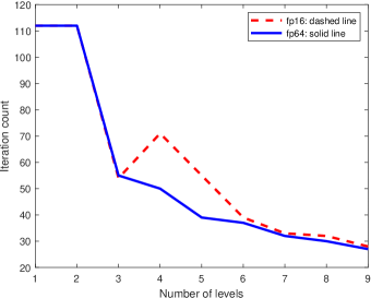
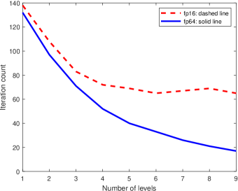
Figure 4.1: IC-CG-IR total iteration counts for the fp16+$IC(\ell)$ preconditioner (dashed line) and fp64+$IC(\ell)$ preconditioner (solid line) with $l$ ranging from 1 to 9 for problems UTEP/Dubcova2 (left) and Cylshell/s2rmt3m1 (right).

Table 4.7: Results for IC-CG-IR using an $IC(3)$ preconditioner: well-conditioned problems. $resint$ and $resfinal$ are the initial and final residuals. $nnz(L)$ is the number of entries in the $IC(3)$ factor. $iouter$ and $totits$ denote the number of outer iterations and the total number of CG iterations, respectively. $>1000$ indicates CG tolerance not reached on outer iteration $iouter$. $nmod$ denotes the number of times problem B1 occurs during the factorization (for fp64-$IC(3)$ it is equal to 0 for all our test cases and so omitted). A count in bold indicates the fp16 result is within 10 per cent of (or is better than) the corresponding fp64 result.

Preconditioner fp16-$IC(3)$
Identifier	$resinit$	$resfinal$	$nnz(L)$	$iouter$	$totits$	$nmod$
HB/bcsstk27	8.27$\times 10^{-5}$	1.23$\times 10^{-15}$	4.88$\times 10^{4}$	3	11	0
Nasa/nasa2146	9.07$\times 10^{-5}$	7.41$\times 10^{-15}$	7.89$\times 10^{4}$	3	11	0
Cylshell/s1rmq4m1	5.81$\times 10^{-5}$	1.05$\times 10^{-14}$	3.15$\times 10^{5}$	3	47	0
MathWorks/Kuu	1.74$\times 10^{-4}$	8.21$\times 10^{-15}$	7.65$\times 10^{5}$	3	33	0
Pothen/bodyy6	7.39$\times 10^{-3}$	1.40$\times 10^{-16}$	1.76$\times 10^{5}$	4	108	2
GHS$\_$psdef/wathen120	4.34$\times 10^{-4}$	6.69$\times 10^{-16}$	8.30$\times 10^{5}$	3	6	0
GHS$\_$psdef/jnlbrng1	1.41$\times 10^{-3}$	5.10$\times 10^{-15}$	2.77$\times 10^{5}$	3	12	0
Williams/cant	3.28$\times 10^{-4}$	3.74$\times 10^{-15}$	9.95$\times 10^{6}$	3	1103	0
UTEP/Dubcova2	1.54$\times 10^{-3}$	1.88$\times 10^{-13}$	6.22$\times 10^{6}$	3	54	0
Cunningham/qa8fm	3.54$\times 10^{-4}$	1.04$\times 10^{-16}$	5.14$\times 10^{6}$	3	6	0
Mulvey/finan512	3.50$\times 10^{-4}$	4.97$\times 10^{-17}$	4.08$\times 10^{6}$	3	6	0
GHS$\_$psdef/apache1	8.51$\times 10^{-5}$	3.65$\times 10^{-14}$	1.54$\times 10^{6}$	2	116	0
Williams/consph	1.04$\times 10^{-4}$	1.57$\times 10^{-14}$	2.02$\times 10^{7}$	3	160	0
AMD/G2$\_$circuit	8.15$\times 10^{-4}$	3.28$\times 10^{-16}$	1.04$\times 10^{6}$	4	282	0
Preconditioner fp64-$IC(3)$
Identifier	$resinit$	$resfinal$	$nnz(L)$	$iouter$	$totits$
HB/bcsstk27	3.93$\times 10^{-5}$	3.13$\times 10^{-16}$	4.88$\times 10^{4}$	3	8
Nasa/nasa2146	4.32$\times 10^{-5}$	8.80$\times 10^{-16}$	7.89$\times 10^{4}$	3	11
Cylshell/s1rmq4m1	3.55$\times 10^{-5}$	1.66$\times 10^{-15}$	3.15$\times 10^{5}$	3	56
MathWorks/Kuu	2.50$\times 10^{-4}$	2.25$\times 10^{-15}$	7.65$\times 10^{5}$	3	30
Pothen/bodyy6	9.31$\times 10^{-3}$	1.40$\times 10^{-16}$	1.76$\times 10^{5}$	4	63
GHS$\_$psdef/wathen120	1.77$\times 10^{-4}$	9.56$\times 10^{-17}$	8.30$\times 10^{5}$	3	6
GHS$\_$psdef/jnlbrng1	9.40$\times 10^{-4}$	3.22$\times 10^{-16}$	2.77$\times 10^{5}$	3	12
Williams/cant	3.19$\times 10^{-4}$	6.09$\times 10^{-15}$	9.95$\times 10^{6}$	3	927
UTEP/Dubcova2	1.65$\times 10^{-3}$	1.84$\times 10^{-13}$	6.22$\times 10^{6}$	3	55
Cunningham/qa8fm	3.29$\times 10^{-5}$	1.24$\times 10^{-16}$	5.14$\times 10^{6}$	3	5
Mulvey/finan512	3.72$\times 10^{-5}$	6.63$\times 10^{-17}$	4.08$\times 10^{6}$	3	6
GHS$\_$psdef/apache1	8.28$\times 10^{-5}$	4.12$\times 10^{-14}$	1.54$\times 10^{6}$	2	120
Williams/consph	3.39$\times 10^{-4}$	6.07$\times 10^{-3}$	2.02$\times 10^{7}$	1	$>1000$
AMD/G2$\_$circuit	8.42$\times 10^{-5}$	2.46$\times 10^{-16}$	1.04$\times 10^{6}$	4	273

Table 4.8: Results for IC-CG-IR and IC-GMRES-IR using an $IC(3)$ preconditioner: ill-conditioned problems. $resint$ is the initial residual; $resfinal$ is the final IC-CG-IR scaled residual. $nnz(L)$ is the number of entries in the $IC(3)$ factor. $iouter$ and $totits$ denote the number of outer iterations and the total number of CG iterations with the GMRES statistics in parentheses. $>1000$ indicates CG (or GMRES) tolerance not reached on outer iteration $iouter$. $nmod$ and $nofl$ denote the numbers of times problems B1 and $B3$ occur during the factorization (for fp64-$IC(3)$ they are equal to 0 for all our test cases and so omitted). A count in bold indicates the fp16 result is within 10 per cent (or better) of the corresponding fp64 result. ‡ indicates failure to compute the factorization because of enormous growth in its entries.

Preconditioner fp16-$IC(3)$
Identifier	$resinit$	$resfinal$	$nnz(L)$	$iouter$	$totits$		$nmod$	$nofl$
Boeing/msc01050	1.61$\times 10^{-3}$	6.47$\times 10^{-14}$	3.74$\times 10^{4}$	3	125	(64)	2	0
HB/bcsstk11	5.84$\times 10^{-4}$	1.89$\times 10^{-13}$	4.18$\times 10^{4}$	3	265	(184)	0	2
HB/bcsstk26	6.42$\times 10^{-5}$	1.51$\times 10^{-13}$	3.43$\times 10^{4}$	3	80	(70)	2	0
HB/bcsstk24	5.91$\times 10^{-7}$	1.77$\times 10^{-13}$	2.27$\times 10^{5}$	3	437	(260)	0	2
HB/bcsstk16	6.16$\times 10^{-4}$	6.64$\times 10^{-15}$	4.89$\times 10^{5}$	3	17	(17)	0	0
Cylshell/s2rmt3m1	9.24$\times 10^{-6}$	4.11$\times 10^{-15}$	2.60$\times 10^{5}$	3	83	(117)	0	0
Cylshell/s3rmt3m1	1.72$\times 10^{-6}$	9.01$\times 10^{-15}$	2.60$\times 10^{5}$	3	386	(504)	1	1
Boeing/bcsstk38	1.07$\times 10^{-3}$	1.43$\times 10^{-15}$	5.64$\times 10^{5}$	4	$1004$	(282)	2	0
Boeing/msc10848	5.97$\times 10^{-7}$	1.13$\times 10^{-14}$	2.51$\times 10^{6}$	3	138	(89)	0	0
Oberwolfach/t2dah$\_$e	6.81$\times 10^{-4}$	1.88$\times 10^{-16}$	3.29$\times 10^{5}$	3	6	(6)	0	0
Boeing/ct20stif	2.78$\times 10^{-5}$	1.63$\times 10^{-9}$	6.70$\times 10^{6}$	3	$>1000$	($>1000$)	2	0
DNVS/shipsec8	5.56$\times 10^{-6}$	1.26$\times 10^{-16}$	1.22$\times 10^{7}$	4	$2067$	($1399$)	2	0
Um/2cubes$\_$sphere	1.02$\times 10^{-3}$	1.63$\times 10^{-16}$	8.70$\times 10^{6}$	3	6	(6)	0	0
GHS$\_$psdef/hood	6.80$\times 10^{-4}$	5.01$\times 10^{-17}$	2.78$\times 10^{7}$	4	444	(406)	0	4
Um/offshore	1.53$\times 10^{-3}$	1.38$\times 10^{-13}$	2.08$\times 10^{7}$	3	103	(40)	0	4
Preconditioner fp64-$IC(3)$
Identifier	$resinit$	$resfinal$	$nnz(L)$	$iouter$	$totits$
Boeing/msc01050	1.41$\times 10^{-4}$	5.80$\times 10^{-14}$	3.74$\times 10^{4}$	3	38	(25)
HB/bcsstk11	1.48$\times 10^{-5}$	6.96$\times 10^{-14}$	4.18$\times 10^{4}$	3	29	(29)
HB/bcsstk26	9.24$\times 10^{-5}$	1.68$\times 10^{-13}$	3.43$\times 10^{4}$	3	60	(62)
HB/bcsstk24	4.01$\times 10^{-7}$	1.01$\times 10^{-13}$	2.27$\times 10^{5}$	3	71	(67)
HB/bcsstk16	7.01$\times 10^{-4}$	3.13$\times 10^{-15}$	4.89$\times 10^{5}$	3	15	(14)
Cylshell/s2rmt3m1	8.61$\times 10^{-6}$	8.74$\times 10^{-15}$	2.60$\times 10^{5}$	3	71	(105)
Cylshell/s3rmt3m1	2.00$\times 10^{-6}$	6.12$\times 10^{-5}$	2.60$\times 10^{5}$	1	$>1000$	($>1000$)
Boeing/bcsstk38	4.67$\times 10^{-9}$	8.34$\times 10^{-14}$	5.64$\times 10^{5}$	3	154	115)
Boeing/msc10848	8.73$\times 10^{-10}$	2.26$\times 10^{-16}$	2.51$\times 10^{6}$	3	47	(46)
Oberwolfach/t2dah$\_$e	5.49$\times 10^{-6}$	6.54$\times 10^{-16}$	3.29$\times 10^{5}$	3	5	(5)
Boeing/ct20stif	5.82$\times 10^{-8}$	2.02$\times 10^{-11}$	6.70$\times 10^{6}$	3	$>1000$	($>1000$)
DNVS/shipsec8	7.50$\times 10^{-7}$	1.11$\times 10^{-16}$	1.22$\times 10^{7}$	4	313	(181)
Um/2cubes$\_$sphere	2.25$\times 10^{-5}$	1.63$\times 10^{-16}$	8.70$\times 10^{6}$	3	5	(5)
GHS$\_$psdef/hood	‡	‡	‡	‡	‡	‡
Um/offshore	‡	‡	‡	‡	‡	‡

Tables 4.7 and 4.8 present results for IC-CG-IR with the fp16-$IC(3)$ and fp64-$IC(3)$ preconditioners for the well-conditioned and ill-conditioned test sets, respectively. The latter also reports total iteration counts for IC-GMRES-IR (the number of outer iterations $iouter$ for IC-GMRES-IR and IC-CG-IR are the same for all the test examples). In double precision arithmetic, B1 breakdowns do not happen for any of our test cases and so the $nmod$ statistic is omitted. B3 breakdowns occur for a small number of the ill-conditioned problems. We see that, for our examples, the number of entries in $L$ is (approximately) the same for both fp16 and fp64 arithmetic, indicating that (in contrast to $IC(0)$) the number of subnormal numbers is small. fp16-$IC(3)$ performs as well as fp64-$IC(3)$ on most of the well-conditioned problems. Note that for problem Williams/consph the required accuracy was not achieved using fp64 on the first outer iteration. For the ill-conditioned problems, while the fp16-$IC(3)$ preconditioner combined with IC-CG-IR and IC-GMRES-IR is able to return a computed solution with a small residual, for the problems for which B1 and/or B3 are detected in fp16 arithmetic the iteration counts are significantly greater than for the fp64-$IC(3)$ preconditioner (see, for instance, Boeing/msc01050 and HB/bcsstk11). This is because the use of shifts to prevent breakdowns means the computed factors are for a shifted matrix. However, for a small number of problems the computation of the fp64-$IC(3)$ preconditioner fails because the computed factor has very large entries, which do not overflow in double precision but make it useless as a preconditioner. This indicates that it is not just in half precision arithmetic that it is necessary to monitor the possibility of growth occurring in the factor entries, something that is not currently considered when computing incomplete Cholesky factorizations in double (or single) precision arithmetic.

Note that, when using fp16 arithmetic, the initial residual $resint$ is typically larger than for fp64 arithmetic. However, if double precision accuracy in the computed solution is not required, performing refinement may be unnecessary (or a small number of steps may be sufficient), even for fp16 incomplete factors.

5 Concluding remarks and future directions

The focus of this study is the construction and employment of incomplete factorizations using half precision arithmetic to solve large-scale sparse linear systems to double precision accuracy. Our experiments, which simulate half precision arithmetic through the use of the NAG compiler demonstrate that, when carefully implemented, the use of fp16 level-based incomplete factorization preconditioners may not impact on the overall accuracy of the computed solution, even when a small tolerance is imposed on the requested scaled residual. Unsurprisingly, the number of iterations of the Krylov subspace method that is used in the refinement process can be greater for fp16 factors compared to fp64 factors but generally this increase is only significant for highly ill-conditioned systems. Our results support the view that, for many real-world problems, it is sufficient to employ half precision arithmetic. Its use may be particularly advantageous if the linear system does not need to be solved to high accuracy. Our study also encourages us to conjecture that by building safe operations into sparse direct solvers it should be possible to build efficient and robust half precision variants and, because this would lead to substantial memory savings for the matrix factors, it could potentially allow direct solvers to be used (in combination with an appropriate refinement process) to solve much larger problems than is currently possible. This is a future direction that is becoming more feasible to explore as compiler support for fp16 arithmetic improves and becomes available on more platforms and for more languages.

It is of interest to consider other Krylov solvers such as flexible CG and flexible GMRES and to explore other classes of algebraic preconditioners, to consider how they can be safely computed using fp16 arithmetic and how effective they are compared to higher precision versions. For sparse approximate inverse (SPAI) preconditioners, we anticipate that it may be possible to combine the systematic dropping of subnormal quantities with avoiding overflows in local linear solves as we have discussed without significantly affecting the preconditioner quality because such changes may only influence a small number of the computed columns of the SPAI preconditioner (see also [Carson and Khan(2023)] for a recent analysis of SPAI preconditioners in mixed precision). For other approximate inverses, such as AINV [Benzi et al.(1996)] and AIB [Saad(2003)], the sizes of the diagonal entries follow from maintaining a generalized orthogonalization property and avoiding overflows using local or global modifications may be possible but challenging. We also plan to consider the construction of the HSL_MI28 [Scott and Tuma(2014)] IC preconditioner using low precision arithmetic. HSL_MI28 uses an extended memory approach for the robust construction of the factors. Once the factors have been computed, the extended memory can be freed, limiting the size of the factors and the work needed in the substitution steps, generally without a significant reduction in the preconditioner quality. A challenge here is safely allowing intermediate quantities of absolute value at least $x_{min}$ to be retained in the factors or in the extended memory.

Acknowledgements We are very grateful to the anonymous reviewers for their detailed comments that have led to significant improvements to this paper.

References

- [1]
- [Abdelfattah et al.(2021)] A. Abdelfattah, H. Anzt, E. G. Boman, E. Carson, T. Cojean, J. Dongarra, A. Fox, M. Gates, N. J. Higham, X. S. Li, J. Loe, P. Luszczek, S. Pranesh, S. Rajamanickam, T. Ribizel, B. F. Smith, K. Swirydowicz, S. Thomas, S. Tomov, Y. M. Tzai, and U. Meier Yang. 2021. A survey of numerical linear algebra methods utilizing mixed-precision arithmetic. International J. High Performance Computing Applications 35, 4 (2021), 344–369.
- [Amestoy et al.(2021)] P. Amestoy, A. Buttari, N. J. Higham, J.-Y. L’Excellent, T. Mary, and B. Vieuble. 2021. Five-Precision GMRES-based iterative refinement. Technical Report MIMS EPrint: 2021.5. Manchester Institute for Mathematical Sciences, University of Manchester.
- [Amestoy et al.(2023)] P. Amestoy, A. Buttari, N. J. Higham, J.-Y. L’Excellent, T. Mary, and B. Vieuble. 2023. Combining sparse approximate factorizations with mixed precision iterative refinement. ACM Trans. Math. Software 49, 1 (2023), 4:1–4:28.
- [Amestoy et al.(2000)] P. R. Amestoy, I. S. Duff, and J-Y L’Excellent. 2000. Multifrontal parallel distributed symmetric and unsymmetric solvers. Computer methods in applied mechanics and engineering 184, 2-4 (2000), 501–520.
- [Arioli and Duff(2009)] M. Arioli and I. S Duff. 2009. Using FGMRES to obtain backward stability in mixed precision. Electronic Transactions on Numerical Analysis 33 (2009), 31–44.
- [Arioli et al.(2007)] M. Arioli, I. S. Duff, S. Gratton, and S. Pralet. 2007. A note on GMRES preconditioned by a perturbed LDLT decomposition with static pivoting. SIAM J. on Scientific Computing 29, 5 (2007), 2024–2044. https://doi.org/10.1137/060661545
- [Baboulin et al.(2009)] M. Baboulin, A. Buttari, J. Dongarra, J. Kurzak, J. Langou, J. Langou, P. Luszczek, and S. Tomov. 2009. Accelerating scientific computations with mixed precision algorithms. Comp. Phys. Comm. 180, 12 (2009), 2526–2533.
- [Benzi(2002)] M. Benzi. 2002. Preconditioning techniques for large linear systems: a survey. J. of Computational Physics 182, 2 (2002), 418–477.
- [Benzi et al.(1996)] M. Benzi, C. D. Meyer, and M. Tuma. 1996. A sparse approximate inverse preconditioner for the conjugate gradient method. SIAM J. on Scientific Computing 17, 5 (1996), 1135–1149.
- [Buttari et al.(2007a)] A. Buttari, J. Dongarra, and J. Kurzak. 2007a. Limitations of the PlayStation 3 for high performance cluster computing. Technical Report MIMS EPrint: 2007.93. Manchester Institute for Mathematical Sciences, University of Manchester.
- [Buttari et al.(2008)] A. Buttari, J. Dongarra, J. Kurzak, P. Luszczek, and S. Tomov. 2008. Using mixed precision for sparse matrix computations to enhance the performance while achieving 64-bit accuracy. ACM Trans. Math. Software 34 (2008), 17:1–17:22.
- [Buttari et al.(2007b)] A. Buttari, J. Dongarra, J. Langou, J. Langou, P. Luszczek, and J. Kurzak. 2007b. Mixed Precision Iterative Refinement Techniques for the Solution of Dense Linear Systems. International J. High Performance Computing Applications 21, 4 (2007), 457–466. https://doi.org/10.1177/1094342007084026
- [Carson et al.(2020)] E. Carson, N. Higham, and S. Pranesh. 2020. Three-Precision GMRES-based Iterative Refinement for Least Squares Problems. SIAM J. on Scientific Computing 42, 6 (2020), A4063–A4083.
- [Carson and Higham(2017)] E. Carson and N. J. Higham. 2017. A new analysis of iterative refinement and its application to accurate solution of ill-conditioned sparse linear systems. SIAM J. on Scientific Computing 39, 6 (2017), A2834–A2856.
- [Carson and Higham(2018)] E. Carson and N. J. Higham. 2018. Accelerating the solution of linear systems by iterative refinement in three precisions. SIAM J. on Scientific Computing 40, 2 (2018), A817–A847.
- [Carson and Khan(2023)] E. Carson and N. Khan. 2023. Mixed Precision Iterative Refinement with Sparse Approximate Inverse Preconditioning. SIAM J. on Scientific Computing (2023). To appear.
- [Chan and van der Vorst(1997)] T. F. Chan and H. A. van der Vorst. 1997. Approximate and incomplete factorizations. In Parallel Numerical Algorithms, ICASE/LaRC Interdisciplinary Series in Science and Engineering IV. Centenary Conference, D.E. Keyes, A. Sameh and V. Venkatakrishnan, eds. Kluver Academic Publishers, Dordrecht, 167–202.
- [Demmel et al.(2006)] J. Demmel, Y. Hida, W. Kahan, X. S. Li, S. Mukherjee, and E. J. Riedy. 2006. Error bounds from extra-precise iterative refinement. ACM Trans. Math. Software 32, 2 (2006), 325–351.
- [Greenbaum(1997)] A. Greenbaum. 1997. Estimating the attainable accuracy of recursively computed residual methods. SIAM J. on Matrix Analysis and Applications 18 (1997), 535–551.
- [Grote and Huckle(1997)] M. J. Grote and T. Huckle. 1997. Parallel preconditioning with sparse approximate inverses. SIAM J. on Scientific Computing 18, 3 (1997), 838–853.
- [Higham(2002)] N. J. Higham. 2002. Accuracy and stability of numerical algorithms. SIAM.
- [Higham and Mary(2022)] N. J. Higham and T. Mary. 2022. Mixed precision algorithms in numerical linear algebra. Acta Numerica 31 (2022), 347–414.
- [Higham and Pranesh(2019)] N. J. Higham and S. Pranesh. 2019. Simulating low precision floating-point arithmetic. SIAM J. on Scientific Computing 41, 5 (2019), C585–C602.
- [Higham and Pranesh(2021)] N. J. Higham and S. Pranesh. 2021. Exploiting lower precision arithmetic in solving symmetric positive definite linear systems and least squares problems. SIAM J. on Scientific Computing 43, 1 (2021), A258–A277.
- [Higham et al.(2019)] N. J. Higham, S. Pranesh, and M. Zounon. 2019. Squeezing a matrix into half precision, with an application to solving linear systems. SIAM J. on Scientific Computing 41, 4 (2019), A2536–A2551. https://doi.org/10.1137/18M1229511
- [Hogg and Scott(2010)] J. D. Hogg and J. A. Scott. 2010. A fast and robust mixed precision solver for sparse symmetric systems. ACM Trans. Math. Software 37, 2 (2010), 1–24. Article 4, 19 pages.
- [HSL(2023)] HSL 2023. HSL. A collection of Fortran codes for large-scale scientific computation. http://www.hsl.rl.ac.uk.
- [Hysom and Pothen(1999)] D. Hysom and A. Pothen. 1999. Efficient parallel computation of ILU(k) preconditioners. In SC ’99: Proceedings of the 1999 ACM/IEEE conference on Supercomputing, Portland, OR. ACM/IEEE, 1–29.
- [Kershaw(1978)] D. S. Kershaw. 1978. The incomplete Cholesky-conjugate gradient method for the iterative solution of systems of linear equations. J. of Computational Physics 26 (1978), 43–65.
- [Knight et al.(2014)] P. A. Knight, D. Ruiz, and B. Uçar. 2014. A symmetry preserving algorithm for matrix scaling. SIAM J. on Matrix Analysis and Applications 35, 3 (2014), 931–955. https://doi.org/10.1137/110825753
- [Kurzak and Dongarra(2007)] J. Kurzak and J. Dongarra. 2007. Implementation of mixed precision in solving systems of linear equations on the CELL processor. Concurrency and Computation: Practice and Experience 19, 10 (2007), 1371–1385.
- [Langou et al.(2006)] J. Langou, Jul. Langou, P. Luszczek, J. Kurzak, A. Buttari, and J. Dongarra. 2006. Exploiting the performance of 32 bit floating point arithmetic in obtaining 64 bit accuracy (revisiting iterative refinement for linear systems). In SC’06: Proceedings of the 2006 ACM/IEEE Conference on Supercomputing. https://doi.org/10.1109/SC.2006.30
- [Lin and Moré(1999)] C.-J. Lin and J. J. Moré. 1999. Incomplete Cholesky factorizations with limited memory. SIAM J. on Scientific Computing 21, 1 (1999), 24–45.
- [Lindquist et al.(2020)] N. Lindquist, P. Luszczek, and J. Dongarra. 2020. Improving the performance of the GMRES method using mixed-precision techniques. In Driving Scientific and Engineering Discoveries Through the Convergence of HPC, Big Data and AI: 17th Smoky Mountains Computational Sciences and Engineering Conference, SMC 2020, Oak Ridge, TN, USA, August 26–28, 2020, Revised Selected Papers 17. Springer, 51–66.
- [Lindquist et al.(2022)] N. Lindquist, P. Luszczek, and J. Dongarra. 2022. Accelerating restarted GMRES with mixed precision arithmetic. IEEE Transactions on Parallel and Distributed Systems 33, 4 (2022), 1027–1037.
- [Loe et al.(2021)] J. A. Loe, C. A. Glusa, I. Yamazaki, E. G. Boman, and S. Rajamanickam. 2021. Experimental evaluation of multiprecision strategies for GMRES on GPUs. In 2021 IEEE International Parallel and Distributed Processing Symposium Workshops (IPDPSW). IEEE, 469–478. https://doi.org/10.1109/IPDPSW52791.2021.00078
- [Manteuffel(1980)] T. A. Manteuffel. 1980. An incomplete factorization technique for positive definite linear systems. Math. Comp. 34 (1980), 473–497.
- [McCormick et al.(2021)] S. F. McCormick, J. Benzaken, and R. Tamstorf. 2021. Algebraic error analysis for mixed-precision multigrid solvers. SIAM J. on Scientific Computing 43, 5 (2021), S392–S419. https://doi.org/10.1137/20M1348571
- [Meijerink and van der Vorst(1977)] J. A. Meijerink and H. A. van der Vorst. 1977. An iterative solution method for linear systems of which the coefficient matrix is a symmetric -matrix. Math. Comp. 31, 137 (1977), 148–162.
- [Ruiz(2001)] D. Ruiz. 2001. A scaling algorithm to equilibrate both rows and columns norms in matrices. Technical Report RAL-TR-2001-034. Rutherford Appleton Laboratory, Chilton, Oxfordshire, England.
- [Ruiz and Uçar(2011)] D. Ruiz and B. Uçar. 2011. A symmetry preserving algorithm for matrix scaling. Technical Report INRIA RR-7552. INRIA, Grenoble, France.
- [Saad(1994)] Y. Saad. 1994. A flexible inner-outer preconditioned GMRES algorithm. SIAM J. on Scientific and Statistical Computing 14 (1994), 461–469.
- [Saad(2003)] Y. Saad. 2003. Iterative Methods for Sparse Linear Systems (second ed.). SIAM, Philadelphia, PA. xviii+528 pages.
- [Scott and Tuma(2014)] J. A. Scott and M. Tuma. 2014. HSL_MI28: an efficient and robust limited-memory incomplete Cholesky factorization code. ACM Trans. Math. Software 40, 4 (2014), 24:1–19.
- [Zounon et al.(2022)] M. Zounon, N. J. Higham, C. Lucas, and F. Tisseur. 2022. Performance impact of precision reduction in sparse linear systems solvers. PeerJ Computer Science 8 (2022), e778:1–22. https://doi.org/10.7717/perrj-cs.778