Gaussian Entanglement Measure:
Applications to Multipartite Entanglement of Graph States and Bosonic Field Theory

Abstract

Computationally feasible multipartite entanglement measures are needed to advance our understanding of complex quantum systems. An entanglement measure based on the Fubini-Study metric has been recently introduced by Cocchiarella and co-workers, showing several advantages over existing methods, including ease of computation, a deep geometrical interpretation, and applicability to multipartite entanglement. Here, we present the Gaussian Entanglement Measure (GEM), a generalization of geometric entanglement measure for multimode Gaussian states, based on the purity of fragments of the whole systems. Our analysis includes the application of GEM to a two-mode Gaussian state coupled through a combined beamsplitter and a squeezing transformation. Additionally, we explore 3-mode and 4-mode graph states, where each vertex represents a bosonic mode, and each edge represents a quadratic transformation for various graph topologies. Interestingly, the ratio of the geometric entanglement measures for graph states with different topologies naturally captures properties related to the connectivity of the underlying graphs. Finally, by providing a computable multipartite entanglement measure for systems with a large number of degrees of freedom, we show that our definition can be used to obtain insights into a free bosonic field theory on $\mathbb{R}_{t}\times S^{1}$, going beyond the standard bipartite entanglement entropy approach between different regions of spacetime. The results presented herein suggest how the GEM paves the way for using quantum information-theoretical tools to study the topological properties of the space on which a quantum field theory is defined.

Introduction

Quantum entanglement stands as a cornerstone in the development of quantum-based technologies due to its significance in the pursuit of quantum supremacy  [1, 2] and enhanced quantum control  [3, 4]. Major advances have been made in characterizing quantum entanglement and its robustness in the mathematical theory of quantum information for both pure and mixed states [5, 6]. Yet, the quantification of entanglement remains an open challenge [7, 8, 9, 10, 11]. Previous efforts to quantify entanglement have primarily focused on entropy measures; for example, in pure and bipartite systems, the entropy of entanglement is widely accepted as a measure of entanglement [12, 13, 14]. Faithful measures for mixed states of the same class of system include the entropy of formation [15], the entropy of distillation [12], and relative entropy of entanglement [7, 16, 17]. However, extending these measures to more general quantum states, particularly for multipartite systems, necessitates the exploration of diverse approaches [18, 19, 20, 21]. Various measures, such as the Schmidt measure [22] and generalizations of concurrence [23], have been proposed for multipartite systems in both pure and mixed states. The demand for a well-defined entanglement measure capable of encompassing multipartite entanglement in both pure and mixed states, applicable to a broad spectrum of systems beyond qubits, has led to the exploration of new methods to derive entanglement measures. In recent years, estimators of quantum entanglement and measures of complexity in multipartite systems have been introduced using results developed within the framework of information geometry, i.e., through the quantum Fisher information [24, 25, 26].
More recently, a geometrical entanglement distance  [27, 28] has been proposed in the form of a well-defined entanglement monotone derived from a scalar quantity obtained for the Fubini-Study metric defined on the projective Hilbert space of the quantum state of a system of $M$ qudit states. This entanglement distance presents numerous advantages: it applies both to pure and mixed states, it can be easily extended to characterize multipartite entanglement for different partitions of the same composite system, it is easier to compute than other entanglement measures (such as the entropy of formation), and it naturally provides a geometrical framework to describe quantum entanglement.
The properties and the analytical form of such a geometrical entanglement metric have been extensively studied for systems of finite-dimensional Hilbert spaces. While, in principle, the entanglement distance can be applied to continuous variable quantum systems, no extensive studies have been done so far in this direction. The present work extends the entanglement distance defined in [27] for investigating multipartite entanglement for multimode bosonic Gaussian states. Among all possible manifolds of states associated with continuous quantum variables, Gaussian states occupy an important role: they are referred to with different names (squeezed coherent states, generalized Slater determinants, ground states of quadratic Hamiltonians, etc.) and are used in a wide range of research fields including quantum information [29, 30, 31, 32], in quantum field theory in curved spacetime [33, 34] and in thermofield dynamics [35, 36]. In particular, Gaussian states constitute a manifold of states in (projective) Hilbert space often used to approximate ground states for complicated Hamiltonians through variational methods [37, 38, 39, 40]. Moreover, many quantum information methods can be analytically applied to Gaussian states (e.g., entanglement entropy [41, 42], logarithmic negativity [43, 44, 45], circuit complexity [46, 47]). Finally, recent studies in mathematical physics have revealed the rich differential geometrical structure of Gaussian states (both for bosons and fermions), clearly enlightening the connection with the theory of Kähler manifolds and generalized group theoretic coherent states [48, 49]. In this work, we extensively use the geometrical language of variational manifold developed in  [48] to introduce the Gaussian Entanglement Measure (GEM), which extends the entanglement distance to the manifold of bosonic Gaussian states. Among the possible interesting applications of our results, we treat the case of a bosonic scalar field in two spacetime dimensions. The interplay between quantum information and quantum field theory is a very active area of research, in particular in the framework of holography [50, 51, 52, 53, 54, 55]. Traditionally, bipartite entanglement measures such as entanglement entropy have been widely employed to explore the quantum entanglement of quantum fields across two disjoint regions in spacetime. Additionally, expanding the range of application of the entanglement distance to Gaussian states would offer a new quantum information theoretical tool for exploring quantum phase transitions in condensed matter systems. Recent research has highlighted the significance of multipartite entanglement measures linked to quantum Fisher information [25, 56] (as the entanglement distance defined in  [27]) in gaining deeper insights into many-body correlations [57, 58], thus paving the way toward comprehension of quantum phase transitions both in quantum spin systems and in conformal field theory [59]. The paper is structured as follows. In Sec. I we will review the definition of entanglement distance given in  [27] within the framework of the geometry of variational manifold presented in [48]. In particular, we will elucidate how the geometric entanglement distance can be naturally introduced as a scalar geometrical invariant on the homogeneous submanifold generated by the group of local operations embedded in a generalized group theoretical coherent state manifold. In Sec.II we will present the derivation of the analytic expression of the geometric entanglement distance to pure bosonic Gaussian states, i.e. introducing the Gaussian Entanglement Measure (GEM), discussing its general properties and how this is related to other known multipartite entanglement measures for Gaussian states. Finally, in Sec.III we present the application of the GEM to what we will refer to as ’graph state’, and to the ground state of a bosonic quantum field theory on two spacetime dimensions.

The Conclusion section provides a discussion on how the results obtained in the paper suggest several natural generalizations, as well as applications concerning the use of the GEM for better understanding graph theoretic properties of multimode Gaussian states, as well as for potentially being able to capture topological properties of the spacetime on which a field theory is put.

Notations:

Lower case Greek letters denote the mode index. Lower case Latin letters denote Lie algebra indices. Upper case Latin letters denote coordinate indices in phase space.

I Entanglement distance from generalized coherent state manifold: general geometric formulation

I.1 Fubini-Study metric on projective Hilbert space

In introducing the geometrical properties of the manifold of generalized coherent state generated by the action of the LU transformation group $\mathcal{L}$, we will strictly follow [48].
Consider a finite quantum system $\mathcal{S}$ constituted by $N$ distinguishable physical elements. The wave function for the isolated $i$-th part belongs to the Hilbert space $\mathcal{H}_{i}$ so that all the wavefunction $|\Psi\rangle$ the of the full system belongs to the Hilbert space $\mathcal{H}_{\mathcal{S}}=\bigotimes_{\mu=1}^{N}\mathcal{H}_{\mu}$.
The quantum state of the total systems is represented by the projective Hilbert space

$$\mathcal{P}(\mathcal{H}_{\mathcal{S}})=(\mathcal{H}_{\mathcal{S}}\setminus\{\bm{0}\})/\sim\,,$$ (1)

where two wavefunctions are equivalent if the multiplication by a complex number relates them

$$|\Psi\rangle\sim|\Psi^{\prime}\rangle\iff\exists\,c\in\mathbb{C}^{*}\ \ \text{such that}\ \ |\Psi\rangle=c|\Psi^{\prime}\rangle\,\,.$$ (2)

The tangent space to the projective Hilbert space at the point $|\Psi\rangle$ be defined as

$$\mathcal{T}_{\Psi}\mathcal{P}=\mathcal{H}_{\mathcal{S}}/\sim\,,$$ (3)

where the following equivalence relation has been introduced

$$|X\rangle\approx|X^{\prime}\rangle\iff\exists\,c\in\mathbb{C}^{*}\ \text{such that}\ |X^{\prime}\rangle=c|X\rangle\,\,.$$ (4)

From such a definition, it follows that the tangent space to a state vector $|\Psi\rangle$ in projective Hilbert space can be identified with the space of orthogonal vectors to $|\Psi\rangle$, i.e.

$$\mathcal{T}_{\Psi}\mathcal{P}(\mathcal{H}_{\mathcal{S}})=\mathcal{H}^{\perp}_{\Psi}=\{|X\rangle\in\mathcal{H}_{\mathcal{S}}\,\,\,|\,\,\,\langle X|\Psi\rangle=0\}\,\,.$$ (5)

We notice that the tangent space to a state vector $|\Psi\rangle$ has the structure of a Hilbert space induced by the Hilbert space structure of $\mathcal{S}$. In fact, a projector $\mathbb{Q}_{\Psi}$ acting on the space of state vector variations $|\delta\Psi\rangle$ at $|\Psi\rangle$ can be introduced such that

$$\mathbb{Q}_{\Psi}|\delta\Psi\rangle=|\delta\Psi\rangle-\dfrac{\langle\Psi|\delta\Psi\rangle}{\langle\Psi|\Psi\rangle}|\Psi\rangle\,\,.$$ (6)

In what follows, we will consider the case of a variational manifold $\mathcal{M}\subset\mathcal{H}_{\mathcal{S}}$ of vector states $|\Psi(\bm{x})\rangle$ parametrized by a set of $N_{\rm par}$ real parameters $\bm{x}\in\mathcal{D}\subseteq\mathbb{R}^{N_{\rm par}}$, the tangent space $\mathcal{T}_{\bm{x}}\mathcal{M}$ at $|\Psi(\bm{x})\rangle$ is spanned by the vectors

$$|V_{\mu}(\bm{x})\rangle=\mathbb{Q}_{\Psi(\bm{x})}\dfrac{\partial}{\partial x^{\mu}}|\Psi(\bm{x})\rangle\,\,.$$ (7)

forming a real basis $|V^{(\Psi)}_{\mu}\rangle$ of $\mathcal{T}_{\Psi}\mathcal{P}(\mathcal{H}_{\mathcal{S}})$. Within this framework, it is possible to show that the inner product on the Hilbert space $\langle\cdot|\cdot\rangle$ induces a real positive-definite metric bilinear structure $g$ on $\mathcal{T}_{\Psi}\mathcal{P}(\mathcal{H}_{\mathcal{S}})$, the well-known Fubini-Study metric, defined as

$$g_{\mu\nu}(\Psi)=\dfrac{2\mathrm{Re}\left(\left\langle\left.V^{(\Psi)}_{\mu}\right|V^{(\Psi)}_{\nu}\right\rangle\right)}{\langle\Psi|\Psi\rangle}\,.$$ (8)

The Fubini-Study metric endows the variational manifold of the Riemannian metric structure. In [27, 28] a multipartite entanglement measure for pure and mixed states of a system $\mathcal{S}_{qd}$ of q-dits have been proposed based on the Riemannian structure induced on the projective Hilbert describing the state of $\mathcal{S}_{qd}$. In the next session, we reviewed this method within the conceptual framework of generalized coherent state manifold. This would allow a straightforward extension to the submanifold of Gaussian states for a system of distinguishable bosonic modes or Majorana fermions.

I.2 Geometry of generalized coherent states of local operations

In this section, we review the geometric entanglement measure introduced in [27], stressing the connection with the geometry of the manifold of the Lie group generalized coherent states.
As extensively discussed in previous works, any entanglement measure is invariant on the set of states $\varrho_{S}/\mathcal{L}$. It has been noted that such a requirement implies that an entanglement measure of a given pure state represented by the wavefunction $|\Psi_{S}\rangle$ can be introduced from the geometrical invariant of the manifold, the orbits $\mathcal{M}^{(\Psi)}_{\mathcal{L}}$ generated by the application of unitary representations of local operations $\mathcal{L}$ to a state $|\Psi_{S}\rangle$.
In the following derivation, we assume that the considered set of local operations is a real Lie group admitting a real algebra $\mathfrak{l}$ and a projective unitary representation $\mathcal{U}$ on $\mathcal{H}$, i.e.

$$\mathcal{U}(g_{1})\mathcal{U}(g_{2})\sim\mathcal{U}(g_{1}g_{2})\,,\qquad g_{1},g_{2}\in\mathcal{L}\,,$$ (9)

where the equivalence class $\sim$ identifies elements of the representation $\mathcal{U}$ that differ for a complex phase factor.
In case of a composed system $\mathcal{S}$, we define for each part a Lie group action $\mathcal{G}_{\mu}$ with an algebra $\mathfrak{g}_{\mu}$, such that the Lie algebra $\mathfrak{g}_{\rm LO}$ of the considered local transformations is the direct sum of the Lie algebras of the Lie groups acting on fragments, i.e. $\mathfrak{g}_{\rm LO}=\oplus_{\mu=1}^{M}\mathfrak{g}_{\mu}$. At this point, it is worth mentioning that, in general, the Lie group of the considered local operations and, consequently, the associated multipartite entanglement will depend on the partition $\mathfrak{P}$ of the $N$ components of the systems $\mathcal{S}$. Considering the finer partitions implies identifying each part of the system with each physical element, i.e. $N=M$. However, a different partition can be chosen in general with $M<N$ and $\mathfrak{P}=\{\mathcal{S}_{1},...,\mathcal{S}_{M}\}$ where $\sqcup_{\mu=1}^{M}\mathcal{S}_{\mu}=\mathcal{S}$. If $\{T_{(\mu,i)}\}_{i=1,...,n_{\mu}}$ is a basis for the algebra $\mathfrak{g}_{\mu}$, the product in the algebra $\mathfrak{g}_{\rm LO}$ is defined by the brackets

$$[T_{(\mu,i)},T_{(\nu,j)}]=\delta_{\mu\nu}[c^{(\mu)}]_{ij}^{k}T^{(\mu)}_{k}\,,$$ (10)

where $[c^{(\mu)}]_{ij}^{k}$ is the structure constant of the algebra $\mathfrak{g}_{\mu}$.
The action of the algebra of the Lie group on the Hilbert space is defined as

$$\hat{T}_{(\mu,i)}=\dfrac{\mathrm{d}}{\mathrm{d}s}\mathcal{U}(e^{isT_{(\mu,i)}})\biggr{|}_{s=0}\,.$$ (11)

The piece-wise local unitary operators are operators of the form $\mathcal{U}_{\rm LO}(g)=\prod_{i=1}^{N}\mathcal{U}^{(\mu)}$ where $\mathcal{U}^{(\mu)}$ act non-trivially only on the Hilbert space $\mathcal{H}_{\mu}$.

The adjoint representation $\mathrm{Ad}_{\mathfrak{M}}(T_{(\mu,i)})$ of the action of a Lie group element $\mathfrak{M}\in\mathcal{G}_{\rm LO}$ on the algebra $\mathfrak{g}_{\rm LO}$ is represented as the linear map:

$$\mathrm{Ad}_{\mathfrak{M}}(T_{(\mu,i)})=\dfrac{\mathrm{d}}{\mathrm{d}s}\mathfrak{M}e^{sT_{(\mu,i)}}\mathfrak{M}^{-1}\biggr{|}_{s=0}$$ (12)

while the action of the algebra $\mathfrak{g}_{\rm LO}$ on itself is given by

$$\mathrm{ad}_{T_{(\mu,i)}}(T_{(\nu,j)})=[T_{(\mu,i)},T_{(\nu,j)}]=\delta_{\mu\nu}[c^{(\mu)}]_{ij}^{k}T_{(\mu,k)}\,.$$ (13)

From the adjoint representations, a bilinear form, the so-called Killing form, can be introduced to the algebra of the group:

$$\kappa_{(\mu,i)(\nu,j)} =\mathrm{Tr}(\mathrm{ad}_{T_{(\mu,i)}}\mathrm{ad}_{T_{(\nu,j)}})$$

$$=\delta_{\mu\nu}(\kappa^{(\mu)})_{ij}[c^{(\mu)}]_{ik}^{l}[c^{(\mu)}]_{jl}^{k}\,.$$ (14)

where $(\kappa^{(\mu)})_{ij}=[c^{(\mu)}]_{ik}^{l}[c^{(\mu)}]_{jl}^{k}$.
Given a representative state $|\phi\rangle$, one can generate the orbit under the (free) group action of $\mathcal{G}$ on $\mathcal{M}$ generating the orbit $\mathcal{M}_{\mathcal{G}\phi}$, i.e.

$$\mathcal{M}_{\mathcal{G}\phi}=\{\mathcal{U}(\mathfrak{M})|\phi\rangle\ |\ \mathfrak{M}\in\mathcal{G}\}/\sim\ \subset\mathcal{P}(\mathcal{H})\,.$$ (15)

A local system of coordinates on $\mathcal{M}_{\mathcal{G}\phi}$ in a neighbor of $\mathcal{U}(\mathfrak{M})|\phi\rangle$ is induced by the exponential map

$$|\mathfrak{M},\bm{s}\rangle=\mathcal{U}\left(e^{i\sum_{\mu=1}^{N}\sum_{i_{\mu}}^{n_{\mu}}s_{(\mu,i_{\mu})}T_{(\mu,i_{\mu})}}\right)|\phi\rangle\,.$$ (16)

so that a basis of tangent vectors $|\mathcal{V}_{(\mu,i)}(\mathfrak{M})\rangle=\mathbb{Q}_{\psi(\mathfrak{M})}\mathcal{M}\hat{T}_{(\mu,i)}|\phi\rangle$ can be defined on the tangent space $\mathcal{T}_{\psi(\mathfrak{M})}\mathcal{M}_{\mathcal{G}\phi}$. The Fubini-Study metric on $\mathcal{P}(\mathcal{H})$ induces a metric structure on the manifold $\mathcal{M}_{\mathcal{G}\phi}$

$$[g(|\psi(\mathfrak{M})\rangle)]_{(\mu,i)(\nu,j)}=\dfrac{2\mathrm{Re}\big{\langle}\left.\mathcal{V}_{(\mu,i)}(|\psi(\mathfrak{M})\rangle)\right|\mathcal{V}_{\nu,j}(|\psi(M)\rangle)\big{\rangle}}{\langle\psi(\mathfrak{M})|\psi(\mathfrak{M})\rangle}\,,$$ (17)

that has the property to be independent on $\mathfrak{M}\in\mathcal{G}$, i.e.

$$(g[\phi])_{(\mu,i)(\nu,j)}=-\dfrac{\langle\phi|\left(\hat{T}_{(\mu,i)}\mathbb{Q}_{\phi}\hat{T}_{(\nu,j)}+\hat{T}_{(\nu,j)}\mathbb{Q}_{\phi}\hat{T}_{(\mu,i)}\right)|\phi\rangle}{2\langle\phi|\phi\rangle}\,.$$ (18)

Using the definition of the projector $\mathbb{Q}_{\phi}$ and assuming $|\delta_{(\mu,j)}\phi\rangle=\hat{T}_{(\nu,j)}|\phi\rangle$, we obtain that

$$\mathbb{Q}_{\phi}\hat{T}_{(\nu,j)}|\phi\rangle=\left(\hat{T}_{(\nu,j)}-\langle\hat{T}_{(\nu,j)}\rangle_{\phi}\right)|\phi\rangle=[\Delta_{\phi}\hat{T}_{(\nu,j)}]|\phi\rangle\,,$$ (19)

and substituting the previous expression into (18) we obtain

$$(g[\phi])_{(\mu,i)(\nu,j)}=$$ (20)

$$=-\dfrac{\left\langle[\Delta_{\phi}\hat{T}_{(\mu,i)}][\Delta_{\phi}\hat{T}_{(\nu,j)}]\right\rangle_{\phi}+(\mu,i)\leftrightarrow(\nu,j)}{2}\,.$$

It can be directly rewritten

$$(g[\phi])_{(\mu,i)(\nu,j)}=-\frac{M_{ij}^{\mu\nu}+M_{ji}^{\nu\mu}}{2}+M_{i}^{\mu}M_{j}^{\nu}\,.$$ (21)

in terms of the first and second moments in state $|\phi\rangle$ of the $\mathfrak{g}_{\rm LO}$ generators

$$M_{i}^{\mu}\stackrel{{\scriptstyle\text{def}}}{{=}}\left\langle\phi\left|T_{(\mu,i)}\right|\phi\right\rangle\,,\ \ \ \ M_{ij}^{\mu\nu}\stackrel{{\scriptstyle\text{def}}}{{=}}\left\langle\phi\left|T_{(\mu,i)}T_{(\nu,j)}\right|\phi\right\rangle\,.$$ (22)

The invariance of the metric tensor $g$ over the manifold $\mathcal{M}_{\mathcal{G}\phi}$. In [27] a measure of entanglement has been proposed, defining a scalar quantity that is invariant under local unitary transformations that can be rewritten as follows using the language introduced in our work

$$\text{GEM}[\phi]=a\sum_{\mu,\nu=1}^{N}\sum_{i=1}^{n_{N_{\mu}}}\sum_{j=1}^{n_{N_{\nu}}}\kappa^{(\mu,i)(\nu,j)}(g[\phi])_{(\mu,i)(\nu,j)}+b\,,$$ (23)

where $a,b\in\mathbb{R}$ are constants that can be fixed to ensure the correct normalization of the entanglement measure, in particular, if $\phi_{\rm sep}$ is a separable state, then $\text{GEM}[\phi_{\rm sep}]=0.\\$ In the next section, we apply this multipartite entanglement definition to multimode bosonic Gaussian states.

II Geometic entanglement distance for pure Gaussian states

II.1 The geometry of Gaussian states manifold

Let us consider an $N$-modes bosonic system defined by the algebra of creation annihilation operators

$$\mathcal{A}_{N}=\{\hat{a}_{1},\hat{a}^{\dagger}_{1},...,\hat{a}_{N},\hat{a}^{\dagger}_{N}\}$$ (24)

satisfying the canonical commutation relation:

$$[a_{\mu},a_{\nu}^{\dagger}]=\delta_{\mu\nu}\,,$$ (25)

and the space of pure states belonging to the (projective) Hilbert space $\mathcal{P}\mathcal{H}_{M}=\bigotimes_{\mu=1}^{N}\mathcal{P}\mathcal{H}_{\mu}$.
It is convenient to introduce the algebra of quadrature operators

$$\{\hat{q}_{1},\hat{p}_{1},...,\hat{q}_{N},\hat{p}_{N}\}=\{\hat{\xi}_{1},...,\hat{\xi}_{2N}\}\,,$$ (26)

that are related to the creation/annihilation operators by the transformation

$$\hat{a}_{\mu}=\frac{\hat{q}_{\mu}+i\hat{p}_{\mu}}{\sqrt{2}}\,,\ \ \ \ \hat{a}_{\nu}^{\dagger}=\frac{\hat{q}_{\nu}-i\hat{p}_{\nu}}{\sqrt{2}}\,.$$ (27)

and satisfying the commutation relations

$$[\hat{q}_{\mu},\hat{p}_{\nu}]=i\delta_{\mu\nu}\,.$$ (28)

For each state $[|\Psi\rangle]\in\mathcal{P}\mathcal{H}_{N}$, we define the $k$-point correlation coefficients

$$\mathcal{C}_{A_{1},\dots,A_{k}}([|\Psi\rangle])=\langle(\hat{\xi}_{A_{1}}-\langle\hat{\xi}_{A_{1}}\rangle_{\Psi})\dots(\hat{\xi}_{A_{k}}-\langle\hat{\xi}_{A_{k}}\rangle_{\Psi})\rangle_{\Psi}\,\,.$$ (29)

where the capital Latin letters runs over the $2N$-dimensional phase space, i.e. $A_{1},...,A_{k}=1,...,2N$. In particular, the 2-point correlation coefficients can be rewritten in terms of the matrices

$$\mathcal{C}_{A,B}=\Gamma_{AB}+\dfrac{i}{2}\,\Omega_{AB}\,,$$ (30)

where we have introduced the

$$\Gamma_{AB}=\dfrac{1}{2}\left\langle\Psi\left|\left\{\hat{\xi}_{A},\hat{\xi}_{B}\right\}\right|\Psi\right\rangle=\dfrac{\mathcal{C}_{AB}+\mathcal{C}_{BA}}{2}\,,$$ (31)

and anti-symmetric (symplectic) matrix determined by the CCR

$$\Omega_{AB}=-i\left\langle\Psi\left|\left[\hat{\xi}_{A},\hat{\xi}_{B}\right]\right|\Psi\right\rangle=-i(\mathcal{C}_{AB}-\mathcal{C}_{BA})\,,$$ (32)

that, according to our conventions, can be rewritten as

$$\Omega=\bigoplus_{\mu=1}^{N}\Omega^{(\mu)}=\bigoplus_{\mu=1}^{N}\begin{pmatrix}0&1\\ -1&0\\ \end{pmatrix}\,.$$ (33)

In what follows, we will consider the set of Gaussian states parametrized by the matrix $\Gamma$ such that

$$\langle\xi_{A}\rangle_{\Gamma}=0\,\,\,\text{for}\,\,A=1,...,2N\quad\text{and}\quad(\Gamma\Omega^{-1})^{2}=-\mathbb{I}\,\,.$$ (34)

A property of the Gaussian states as defined in eq.(34) is that all the $2n+1$-point correlation coefficients vanish while all the $2n$-point correlation coefficients can be expressed in terms of products of the $\Gamma$ matrix.
We indicate the generic Gaussian state as $|\Gamma\rangle$, and whenever unambiguous, we will denote by simple brackets the expectation in state $|\Gamma\rangle$.
A remarkable property of the Gaussian states is the well-known Wick theorem: the $2n$-point functions in state $|\Gamma\rangle$ can be decomposed into the sum of products of 2-point functions

$$\mathcal{C}_{A_{1},\dots,A_{2n}}(\Gamma)=\frac{1}{n!}\sum_{\sigma}\mathcal{C}_{A_{\sigma(1)},A_{\sigma(2)}}\dots\mathcal{C}_{A_{\sigma(2n-1)},A_{\sigma(2n)}}\,,$$ (35)

where the sum is over all the permutations of $2n$ elements such that $\sigma(2i-1)<\sigma(2i)$ for all $i$.

II.2 Generators of Gaussian unitary transformations: single mode case

To estimate the multipartite entanglement distance eq.(23) for a generic multimode bosonic Gaussian state, we need to define the generators of unitary representation of local operations that are automorphisms in the space of bosonic Gaussian states. We assume identifying each part of our system with a single bosonic mode. A group of automorphism admitting unitary representation on the Gaussian state manifold is the group of Gaussian unitary operator generated by a quadratic Hamiltonian of the form

$$\hat{H}=\frac{1}{2}\begin{pmatrix}\hat{a}^{\dagger}&\hat{a}\end{pmatrix}\begin{pmatrix}A&B\\ B^{*}&A\end{pmatrix}\begin{pmatrix}\hat{a}\\ \hat{a}^{\dagger}\end{pmatrix}\,,$$ (36)

with the constraint that $A\in\mathbb{R}$ and $B\in\mathbb{C}$. One can expand it as

$$\hat{H}=2\text{Re}(B)\,\hat{T}_{1}-2\text{Im}(B)\,\hat{T}_{2}+2A\,\hat{T}_{3}\stackrel{{\scriptstyle\text{def}}}{{=}}\bm{n}\cdot\hat{\bm{T}}$$ (37)

where we have defined the generators

$$\hat{T}_{1} =\frac{\hat{a}^{2}+(\hat{a}^{\dagger})^{2}}{4} =\frac{\hat{q}^{2}-\hat{p}^{2}}{4}\,,$$ (38)

$$\hat{T}_{2} =-\frac{\hat{a}^{2}-(\hat{a}^{\dagger})^{2}}{4i} =-\frac{\hat{p}\hat{q}+\hat{q}\hat{p}}{4}\,,$$

$$\hat{T}_{3} =\frac{\hat{a}^{\dagger}\hat{a}+\hat{a}\hat{a}^{\dagger}}{4} =\frac{\hat{q}^{2}+\hat{p}^{2}}{4}\,,$$

and the vector

$$\bm{n}=2\left(\text{Re}(B),-\text{Im}(B),A\right)^{\textsc{t}}\,.$$ (39)

One can check that the generators satisfy the $\mathfrak{sp}(2,\mathbb{R})$ algebra

$$[\hat{T}_{1},\hat{T}_{2}] =-i\hat{T}_{3}\,,$$

$$[\hat{T}_{2},\hat{T}_{3}] =i\hat{T}_{1}\,,$$ (40)

$$[\hat{T}_{3},\hat{T}_{1}] =i\hat{T}_{2}\,.$$

The associated Killing form corresponds to the Lorentzian metric

$$\kappa_{ij}=2\begin{pmatrix}-1&0&0\\ 0&-1&0\\ 0&0&1\end{pmatrix}\,.$$ (41)

We denote the inverse Killing form by $\kappa^{ij}$.

II.3 Exact computation of the metric tensor: derivation of the GEM

To apply the general definition of the GEM in eq.(23) to a multimode pure Gaussian state, it is required to explicitly compute the (non-trivial) metric tensor defined on the Lie subgroup of single-mode local operations discussed above.
This necessitates the estimation of the expectation values expressed in Eq .(22) for both the generators outlined in eq.(38) and their pairwise products, i.e. 2-points and 4-points functions of the $\hat{q}_{\mu},\hat{p}_{\mu}$ that can be easily calculated by Wick theorem in eq. (35). In the particular case of 4-point functions relevant to us, Wick’s theorem gives:

$$\mathcal{C}_{A_{1},A_{2},A_{3},A_{4}} =\mathcal{C}_{A_{1},A_{2}}\mathcal{C}_{A_{3},A_{4}}+\mathcal{C}_{A_{1},A_{3}}\mathcal{C}_{A_{2},A_{4}}$$

$$+\mathcal{C}_{A_{1},A_{4}}\mathcal{C}_{A_{2},A_{3}}\,,$$ (42)

while the two-point function can be expressed in terms of the correlation matrix and the symplectic form as in eq. (30) The metric tensor is then obtained by symmetrizing the connected component of the second moments. The reader will find the explicit expression of these moments in the App. (A). After the dust settles down, we obtain the following components of the metric tensor:

$$(g[\Gamma])_{(\mu,1)(\nu,1)} =\frac{1}{8}\left(-\Gamma_{p_{\mu},p_{\nu}}^{2}+\Gamma_{p_{\mu},q_{\nu}}^{2}+\Gamma_{p_{\nu},q_{\mu}}^{2}-\Gamma_{q_{\mu},q_{\nu}}^{2}\right)-\frac{\delta_{\mu,\nu}}{16}\,,$$ (43)

$$(g[\Gamma])_{(\mu,1)(\nu,2)} =\frac{1}{4}\left(\Gamma_{q_{\mu},q_{\nu}}\Gamma_{p_{\nu},q_{\mu}}-\Gamma_{p_{\mu},p_{\nu}}\Gamma_{p_{\mu},q_{\nu}}\right)\,,$$

$$(g[\Gamma])_{(\mu,1)(\nu,3)} =\frac{1}{8}\left(\Gamma_{p_{\mu},p_{\nu}}^{2}+\Gamma_{p_{\mu},q_{\nu}}^{2}-\Gamma_{p_{\nu},q_{\mu}}^{2}-\Gamma_{q_{\mu},q_{\nu}}^{2}\right)\,,$$

$$(g[\Gamma])_{(\mu,2)(\nu,2)} =\frac{1}{16}\left(-\delta_{\mu,\nu}-4\left(\Gamma_{p_{\mu},q_{\nu}}\Gamma_{p_{\nu},q_{\mu}}+\Gamma_{p_{\mu},p_{\nu}}\Gamma_{q_{\mu},q_{\nu}}\right)\right)\,,$$

$$(g[\Gamma])_{(\mu,1)(\nu,3)} =\frac{1}{4}\left(\Gamma_{p_{\mu},p_{\nu}}\Gamma_{p_{\nu},q_{\mu}}+\Gamma_{q_{\mu},q_{\nu}}\Gamma_{p_{\mu},q_{\nu}}\right)\,,$$

$$(g[\Gamma])_{(\mu,3)(\nu,3)} =\frac{1}{16}\left(\delta_{\mu,\nu}-2\left(\Gamma_{p_{\mu},p_{\nu}}^{2}+\Gamma_{p_{\mu},q_{\nu}}^{2}+\Gamma_{p_{\nu},q_{\mu}}^{2}+\Gamma_{q_{\mu},q_{\nu}}^{2}\right)\right)\,.$$

In particular, contracting with the Killing form, we have:

$$\text{GEM}[\Gamma] =a\sum_{i,j,\mu,\nu}k^{(\mu,i)(\nu,j)}(g[\Gamma])_{(\mu,i)(\nu,j)}+b$$

$$=a\sum_{i,j,\mu}\kappa^{ij}(g[\Gamma])_{(\mu,i)(\mu,j)}+b$$

$$=\frac{a}{8}\sum_{\mu=1}^{N}\left[\text{det}\left(\Gamma^{(\mu)}\right)-\frac{3}{4}\right]+b\,,$$ (44)

where the reduced density correlation matrix is defined as

$$\Gamma^{(\mu)}=\begin{pmatrix}\Gamma_{q_{\mu},q_{\mu}}&\Gamma_{q_{\mu},p_{\mu}}\\ \Gamma_{p_{\mu},q_{\mu}}&\Gamma_{p_{\mu},p_{\mu}}\end{pmatrix}\,.$$ (45)

To fix the normalization parameters $a$ and $b$, we note that for pure single-mode Gaussian states the eq.(34) reads

$$\Gamma^{(\mu)}[\Omega^{(\mu)}]^{-1}=J^{(\mu)}\quad\text{and}\quad[J^{(\mu)}]^{2}=-\mathbb{1}\,.$$ (46)

From the previous definitions, it follows that

$$(G^{(\mu)}[\Omega^{(\mu)}]^{-1})^{2}=\left[\begin{array}[]{cc}(\mathcal{C}_{q_{\mu},p_{\mu}}+\mathcal{C}_{p_{\mu},q_{\mu}})^{2}-4\mathcal{C}_{q_{\mu},q_{\mu}}\mathcal{C}_{p_{\mu},p_{\mu}}&0\\ 0&(\mathcal{C}_{q_{\mu},p_{\mu}}+\mathcal{C}_{p_{\mu},q_{\mu}})^{2}-4\mathcal{C}_{q_{\mu},q_{\mu}}\mathcal{C}_{p_{\mu},p_{\mu}}\\ \end{array}\right]\overset{!}{=}-\mathbb{1}\,,$$ (47)

from which the following conditions for 2-point functions follow

$$4\mathcal{C}_{q_{\mu},q_{\mu}}\mathcal{C}_{p_{\mu},p_{\mu}}-(\mathcal{C}_{q_{\mu},p_{\mu}}+\mathcal{C}_{p_{\mu},q_{\mu}})^{2}=1\,,$$ (48)

or, equivalently, in terms of the correlation matrix:

$$\Gamma_{p_{\mu},q_{\mu}}^{2}=\Gamma_{q_{\mu},q_{\mu}}\Gamma_{p_{\mu},p_{\mu}}-\frac{1}{4}\,.$$ (49)

Therefore, one has for a separable state (setting here $a=1$ and $b=0$)

$$\text{GEM}[\Gamma_{\text{separable}}]=\frac{N}{8}\,.$$ (50)

Therefore, setting $a=1$ and $b=-\text{GEM}[\Gamma_{\text{separable}};1,0]$, the Gaussian Entanglement Measure of a pure $M$-mode Gaussian state is then given by:

$$\text{GEM}[\Gamma]=\frac{1}{8}\sum_{\mu=1}^{N}\left[\text{det}\left(\Gamma^{(\mu)}\right)-\frac{1}{4}\right]\,.$$ (51)

Let us recall that the purity of a quantum state described by the density matrix $\rho$ is defined as $P\left(\rho\right)=\text{tr}\left(\rho^{2}\right)$. For a Gaussian state identified by the covariance matrix $\Gamma$, the purity can be simply expressed [60] as:

$$P\left(\rho\right)=\frac{1}{2\sqrt{\text{det}\left(\Gamma\right)}}\,.$$ (52)

Hence, the GEM can be rewritten in terms of the purities of the subsystems:

$$\text{GEM}[\Gamma]=\frac{1}{32}\sum_{\mu=1}^{N}\left[\frac{1}{P\left(\rho^{(\mu)}\right)^{2}}-1\right]\,.$$ (53)

It can be very interestingly noticed that another quantity known as the ’potential of multipartite entanglement’ $\pi_{\text{ME}}$ [61, 62], appears to be defined as an average of the purity over partitions of a quantum state into subsystems, $\pi_{\text{ME}}\propto\sum_{\mu}P(\rho^{(\mu)})$. Our approach can be viewed as providing a first-principles motivation for introducing the average purity of the subsystems. Note that by linearity, one can subtract away the contribution of separable states already at the level of the full metric tensor by defining $h[\Gamma]\stackrel{{\scriptstyle\text{def}}}{{=}}g[\Gamma]-g[\Gamma_{\text{separable}}]$ with the following non-zero components:

$$(h[\Gamma])_{(\mu,1)(\nu,1)} =\frac{1}{8}\left(-\Gamma_{p_{\mu},p_{\nu}}^{2}+\Gamma_{p_{\mu},q_{\nu}}^{2}+\Gamma_{p_{\nu},q_{\mu}}^{2}-\Gamma_{q_{\mu},q_{\nu}}^{2}+\left(\Gamma_{p_{\mu},p_{\mu}}-\Gamma_{q_{\mu},q_{\mu}}\right){}^{2}+1-\frac{\delta_{\mu,\nu}}{2}\right)\,,$$ (54)

$$(h[\Gamma])_{(\mu,1)(\nu,2)} =\frac{1}{4}\left(-\Gamma_{p_{\mu},p_{\nu}}\Gamma_{p_{\mu},q_{\nu}}+\Gamma_{q_{\mu},q_{\nu}}\Gamma_{p_{\nu},q_{\mu}}+\Gamma_{p_{\mu},q_{\mu}}\left(\Gamma_{p_{\mu},p_{\mu}}-\Gamma_{q_{\mu},q_{\mu}}\right)\right)\,,$$

$$(h[\Gamma])_{(\mu,1)(\nu,3)} =\frac{1}{8}\left(\Gamma_{p_{\mu},p_{\nu}}^{2}-\Gamma_{p_{\mu},p_{\mu}}^{2}+\Gamma_{p_{\mu},q_{\nu}}^{2}-\Gamma_{p_{\nu},q_{\mu}}^{2}-\Gamma_{q_{\mu},q_{\nu}}^{2}+\Gamma_{q_{\mu},q_{\mu}}^{2}\right)\,,$$

$$(h[\Gamma])_{(\mu,2)(\nu,2)} =\frac{1}{4}\left(-\Gamma_{p_{\mu},q_{\nu}}\Gamma_{p_{\nu},q_{\mu}}-\Gamma_{p_{\mu},p_{\nu}}\Gamma_{q_{\mu},q_{\nu}}+2\Gamma_{p_{\mu},p_{\mu}}\Gamma_{q_{\mu},q_{\mu}}-\frac{\delta_{\mu,\nu}}{4}\right)\,,$$

$$(h[\Gamma])_{(\mu,2)(\nu,3)} =\frac{1}{4}\left(\Gamma_{p_{\mu},p_{\nu}}\Gamma_{p_{\nu},q_{\mu}}+\Gamma_{q_{\mu},q_{\nu}}\Gamma_{p_{\mu},q_{\nu}}-\Gamma_{p_{\mu},q_{\mu}}\left(\Gamma_{p_{\mu},p_{\mu}}+\Gamma_{q_{\mu},q_{\mu}}\right)\right)\,,$$

$$(h[\Gamma])_{(\mu,3)(\nu,3)} =\frac{1}{16}\left(-\Gamma_{p_{\mu},p_{\nu}}^{2}-\Gamma_{p_{\mu},q_{\nu}}^{2}-\Gamma_{p_{\nu},q_{\mu}}^{2}-\Gamma_{q_{\mu},q_{\nu}}^{2}+\left(\Gamma_{p_{\mu},p_{\mu}}+\Gamma_{q_{\mu},q_{\mu}}\right){}^{2}-1+\frac{\delta_{\mu,\nu}}{2}\right)\,.$$

The GEM is then simply given by contraction with the inverse of the Killing metric as before:

$$\text{GEM}[\Gamma] =\sum_{i,j,\mu,\nu}k^{(\mu,i)(\nu,j)}(h[\Gamma])_{(\mu,i)(\mu,j)}$$ (55)

$$=\frac{1}{32}\sum_{\mu=1}^{N}\left[\frac{1}{P\left(\rho^{(\mu)}\right)^{2}}-1\right]\,.$$

Let us mention at this point that we could actually choose to normalize the GEM slightly differently, in particular by dividing by a global factor of $N$, giving the GEM the interpretation of an arithmetic average over the subsystems. We do not choose such a normalization here, but we refer the reader to the end of Sec. III.2 for another comment about this other possible choice of normalization.

II.4 Properties satisfied by GEM

Generic entanglement measures are required to satisfy axioms [63, 27, 64, 65], that we check below for our GEM measure.

Invariance under local unitaries:

This property is natural given the construction. By definition, our quantity only depends on the state up to single-mode unitary transformations.

Positivity:

This property is obvious from the expression (53) in terms of the purity.

Upper bound:

Due to the non-compactness of $\text{Sp}(2M,\mathbb{R})$, one should not expect our definition to admit an upper bound. We refer the reader to Sec. III.1.1 below for a comment concerning a possible way to modify the GEM to make it upper-bounded.

Upper bound attained by maximally entangled states:

The states playing the role of the maximally entangled Bell states correspond in the continuous variable setting to non-normalizable states of the form $\sum_{n}|n\rangle\otimes\dots\otimes|n\rangle$, for which will see in Sec. III.1.1 that indeed their GEM diverges.

Vanishes on separable states:

By construction of the metric tensor $h$, eq. (54), the GEM attains its lower bound for separable states.

III Examples

Generic families of multi-mode Gaussian states are obtained using Hermitian Hamiltonians that are quadratic in the quadratures, or in the creation and annihilation operators. If we define multi-mode generators generalizing their single-mode counterpart (38) as follows:

$$\hat{T}_{1,\mu\nu} =\frac{\hat{a}_{\mu}\hat{a}_{\nu}+\hat{a}_{\mu}^{\dagger}\hat{a}_{\nu}^{\dagger}}{4}\,,$$

$$\hat{T}_{2,\mu\nu} =-\frac{\hat{a}_{\mu}\hat{a}_{\nu}-\hat{a}_{\mu}^{\dagger}\hat{a}_{\nu}^{\dagger}}{4i}\,,$$ (56)

$$\hat{T}_{3,\mu\nu} =\frac{\hat{a}_{\mu}^{\dagger}\hat{a}_{\nu}-\hat{a}_{\mu}\hat{a}_{\nu}^{\dagger}}{4}\,,$$

one can indeed define the following families of $M$-mode Gaussian states:

$$\left|\left\{c_{i,\mu\nu}\right\}\right\rangle\stackrel{{\scriptstyle\text{def}}}{{=}}U\left(\left\{c_{i,\mu\nu}\right\}\right)|0\rangle\stackrel{{\scriptstyle\text{def}}}{{=}}e^{i\hat{H}\left(\left\{c_{i,\mu\nu}\right\}\right)}|0\rangle$$ (57)

with the following generic Hermitian generator:

$$\hat{H}\left(\left\{c_{i,\mu\nu}\right\}\right)=\sum_{\begin{subarray}{c}\mu,\nu=1\\ (\mu<\nu)\end{subarray}}^{N}\sum_{i=1}^{3}c_{i,\mu\nu}\hat{T}_{i,\mu\nu}\,.$$ (58)

and real coefficients $c_{i,\mu\nu}$. For a given number of modes $N$, this family of states is $\tfrac{3N(N-1)}{2}$-dimensional.

For visualization, we will illustrate the GEM for low dimensional sub-families of states which we will call ’graph states’ in what follows.

We also study the case of a massive Klein-Gordon field in two spacetime dimensions to illustrate the applicability of our results to systems with a large number of degrees of freedom.

III.1 Graph states

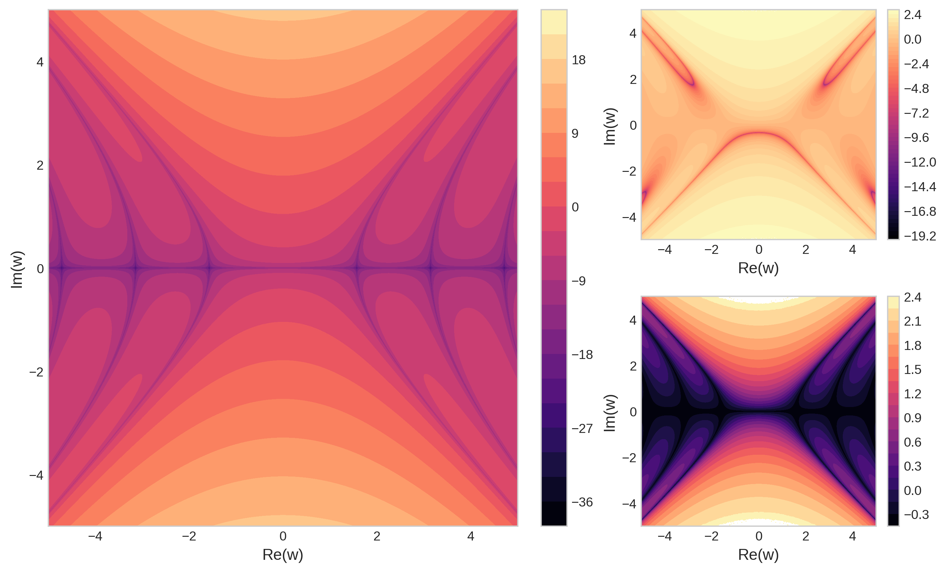
Figure 1: Comparision of our GEM with other well-known measures of entanglement for the two-mode graph states. Left: Logarithm of the Geometric Gaussian Entanglement Measure. Top Right: Logarithm of the Entanglement of Formation. Bottom Right: Logarithm of the Logarithmic Negativity.

Hence, let us introduce a family of multi-mode Gaussian states obtained by setting $c_{1,\mu\nu}=0$ in eq. (58). We also set by convention the remaining variables to

$$c_{3,\mu\nu}\stackrel{{\scriptstyle\text{def}}}{{=}}4\,\text{Re}(A_{\mu\nu})\,,\ \ \ \ \ c_{2,\mu\nu}\stackrel{{\scriptstyle\text{def}}}{{=}}4\,\text{Im}(A_{\mu\nu})\,.$$ (59)

The states are then parameterized by the set of complex numbers $\{A_{\mu\nu}\}$ and given by

$$|\psi\rangle=U\left(\left\{A_{\mu\nu}\right\}\right)|0\rangle\,,$$ (60)

with

$$U\left(\left\{A_{\mu\nu}\right\}\right)=$$ (61)

$$=\text{exp}\left[i\sum_{\begin{subarray}{c}\mu,\nu=1\\ (\mu<\nu)\end{subarray}}^{N}\left(\text{Re}\left(A_{\mu\nu}\right)\hat{a}_{\mu}^{\dagger}\hat{a}_{\nu}+i\text{Im}\left(A_{\mu\nu}\right)\hat{a}_{\mu}\hat{a}_{\nu}+\text{h.c.}\right)\right]\,.$$

The unitary operator generating this $M$-mode state can be expressed in quadrature basis as

$$U\left(\left\{A_{\mu\nu}\right\}\right)=\text{exp}\left[\frac{i}{2}\hat{\bm{\xi}}^{\textsc{t}}h\left(\left\{A_{\mu\nu}\right\}\right)\hat{\bm{\xi}}\right]\,,$$ (62)

with the $h\left(\left\{A_{\mu\nu}\right\}\right)$ matrix being built out of blocks

$$\pNiceMatrix[first-row,first-col]&x_{\nu}p_{\nu}\\ x_{\mu}\text{Re}(A_{\mu\nu})-\text{Im}(A_{\mu\nu})\\ p_{\mu}-\text{Im}(A_{\mu\nu})\text{Re}(A_{\mu\nu})\\ \,,$$ (63)

when $\mu\neq\nu$, and the trivial matrix $\bf 0_{2}$ if $\mu=\nu$. The corresponding symplectic transformation then reads:

$$S\left(\left\{A_{\mu\nu}\right\}\right)=\exp\left[\Omega h\left(\left\{A_{\mu\nu}\right\}\right)\right]\,.$$ (64)

The covariance matrix is again given by

$$\Gamma\left(\left\{A_{\mu\nu}\right\}\right)=\frac{1}{2}\,S\left(\left\{A_{\mu\nu}\right\}\right)S\left(\left\{A_{\mu\nu}\right\}\right)^{\textsc{t}}$$ (65)

The coupling constants $\left\{A_{\mu\nu}\right\}$ are naturally interpreted as the complex weights carried by the edges of a graph connecting the $N$ modes. In what follows, we will treat the case of $N=2$ and $N=3$ node graphs.

III.1.1 Two-mode states

In the particular case of a two-mode state, we denote by $w=A_{12}$ the single coupling appearing in the Hamiltonian. The GEM can be computed exactly as a function of $w$:

$$\text{GEM}[|w\rangle]=\frac{\text{Im}(w)^{2}\sin^{2}\left(2\sqrt{\text{Re}(w)^{2}-\text{Im}(w)^{2}}\right)}{16(\text{Re}(w)^{2}-\text{Im}(w)^{2})}\,.$$ (66)

We refer the reader to fig. (1) (on the left) for a depiction of the GEM as a function of the complex coupling $w$. Two other well-known measures of entanglement for bipartite quantum states are depicted in the same figure: namely, the Entanglement of Formation [66] (computed using the algorithm of [67]) and the Logarithmic Negativity [68]. We observe that the GEM behaves qualitatively like these to other measures. Let us recall that the Entanglement of Formation is notoriously difficult to compute in general, being the solution to a complex optimization problem.

By expressing the complex coupling $w$ in polar coordinates as $w=re^{i\phi}$, one can reexpress the GEM (66) as follows:

$$\text{GEM}[|w\rangle]=\frac{\sin^{2}(\phi)\sin^{2}\left(2r\sqrt{\cos(2\phi)}\right)}{16\cos(2\phi)}\,.$$ (67)

An interesting feature appears in the large squeezing limit. Let us set, for a moment, $\phi=\pm\pi/2$ to turn off the pure beamsplitter component and focus on the two-mode squeezing contribution. In that case, the GEM reduces to:

$$\text{GEM}[|w\rangle]=\frac{1}{16}\sinh^{2}(2r)\,.$$ (68)

One can show [69] that the Schmidt decomposition (over Fock states) of the two-mode squeezed state reads:

$$\exp\left[r\left(a_{1}^{\dagger}a_{2}^{\dagger}-a_{1}a_{2}\right)\right]|0\rangle=\frac{1}{\cosh(r)}\sum_{i\geq 0}\tanh^{i}(r)|i\rangle\otimes|i\rangle\,.$$ (69)

In particular, in the limit of large squeezing $r\to\infty$, this state converges to the balanced superposition of all the states of the form $|i\rangle\otimes|i\rangle$. Though non-normalizable, this state, similarly to EPR states for qubits, corresponds to a maximally entangled state. Once again, this is consistent with the fact that the GEM diverges in the infinite squeezing limit. This observation hints towards a possible new definition of a compact GEM that is, in this case, bounded from above by the entanglement measure of such non-normalizable EPR-like states. Such an upper bound of the entanglement measure can be set to $1$ by convention. For this two-mode example in particular, this can be achieved by bounding the values that can take the modulus of $w$ by substituting, for instance, $r=\tanh(\nu)$, and by normalizing the GEM as follows:

$$\text{GEM}\big{[}\left|\tanh(\nu)e^{i\phi}\right\rangle\big{]}=$$

$$=\frac{1}{2\sinh^{2}(2)}\left[\frac{1}{P\left(\rho^{(1)}\right)^{2}}+\frac{1}{P\left(\rho^{(2)}\right)^{2}}-2\right]\,.$$ (70)

The GEM is then bounded from above by $1$. This regularization can be viewed as effectively compactifying the space of Gaussian states by constraining the possible energy of the states [70, 71] (with respect to a Hamiltonian $\sum_{\mu}\tfrac{p_{\mu}^{2}+q_{\mu}^{2}}{2}$).

Finally, it can be noticed that the full metric tensor can be computed exactly, as can be seen by the interested reader in the App. C.

III.1.2 Three-mode states

In the case of a three-mode state, one can consider two different (connected) graph topologies. Each edge carries a complex weight; therefore, the family of states is 6-dimensional. To visualize the GEM, we reduce the study to two separate 2-dimensional families of states.

Figure 2: Generic complex coupling coefficients.

First family:

For the first family of states, we set all the non-zero complex couplings to be identical, and we consider both the fully connected graph (G1), and the graph with one edge turned off (G2), cf. fig. 3.

Figure 3: First family of three-mode graph states, with identical complex couplings.

The GEM can be expressed explicitely. For G1 we obtain:

$$\text{GEM}_{\text{G}1}\left(w\right)=\frac{\text{Im}(w)^{2}}{12}\frac{\sin^{2}\left(3\sqrt{\text{Re}(w)^{2}-\text{Im}(w)^{2}}\right)}{\text{Re}(w)^{2}-\text{Im}(w)^{2}}$$

$$=\frac{1}{12}\sin^{2}(\phi)\sec(2\phi)\sin^{2}\left(3r\sqrt{\cos(2\phi)}\right)\,,$$ (71)

and for G2:

$$\text{GEM}_{\text{G}2}\left(w\right) =\frac{\text{Im}(w)^{2}\sin^{2}\left(\sqrt{2}\sqrt{\text{Re}(w)^{2}-\text{Im}(w)^{2}}\right)\left(3\cos\left(2\sqrt{2}\sqrt{\text{Re}(w)^{2}-\text{Im}(w)^{2}}\right)+5\right)}{32\left(\text{Re}(w)^{2}-\text{Im}(w)^{2}\right)}$$ (72)

$$=\frac{1}{32}\sin^{2}(\phi)\sec(2\phi)\sin^{2}\left(r\sqrt{\sin(4\phi)\csc(2\phi)}\right)\left(3\cos\left(2r\sqrt{\sin(4\phi)\csc(2\phi)}\right)+5\right)$$

Note that the full metric tensor can be computed for both graphs and is provided for completeness in the App. C.

In fig. (4) we depict the logarithm of the GEM for these two cases, as well as the ratio of the GEM of graph 2 and graph 1. The first observation concerns the fact that a purely real coupling does not generate entanglement. To proceed with interpreting the results, it is fruitful to consider the graph weights to be all proportional to a common time parameter $t$. Therefore, an increase in the amplitude of the couplings corresponds to time evolution. Within this picture, the state preparation provided in eq. (60) can naturally be interpreted as the unitary time evolution given by eq. (60) of an initial state corresponding to the tensor product of Fock vacua under. Equipped with this interpretation, the comparison of the GEM for the two graph topologies becomes clear and compatible with a first intuition: the fully connected graph allows for a faster entanglement. However, for long times, the two GEM become identical, as can be seen in fig. (3) (on the right), indicating that the logarithm of their ratio tends to zero for large amplitudes of $w$.

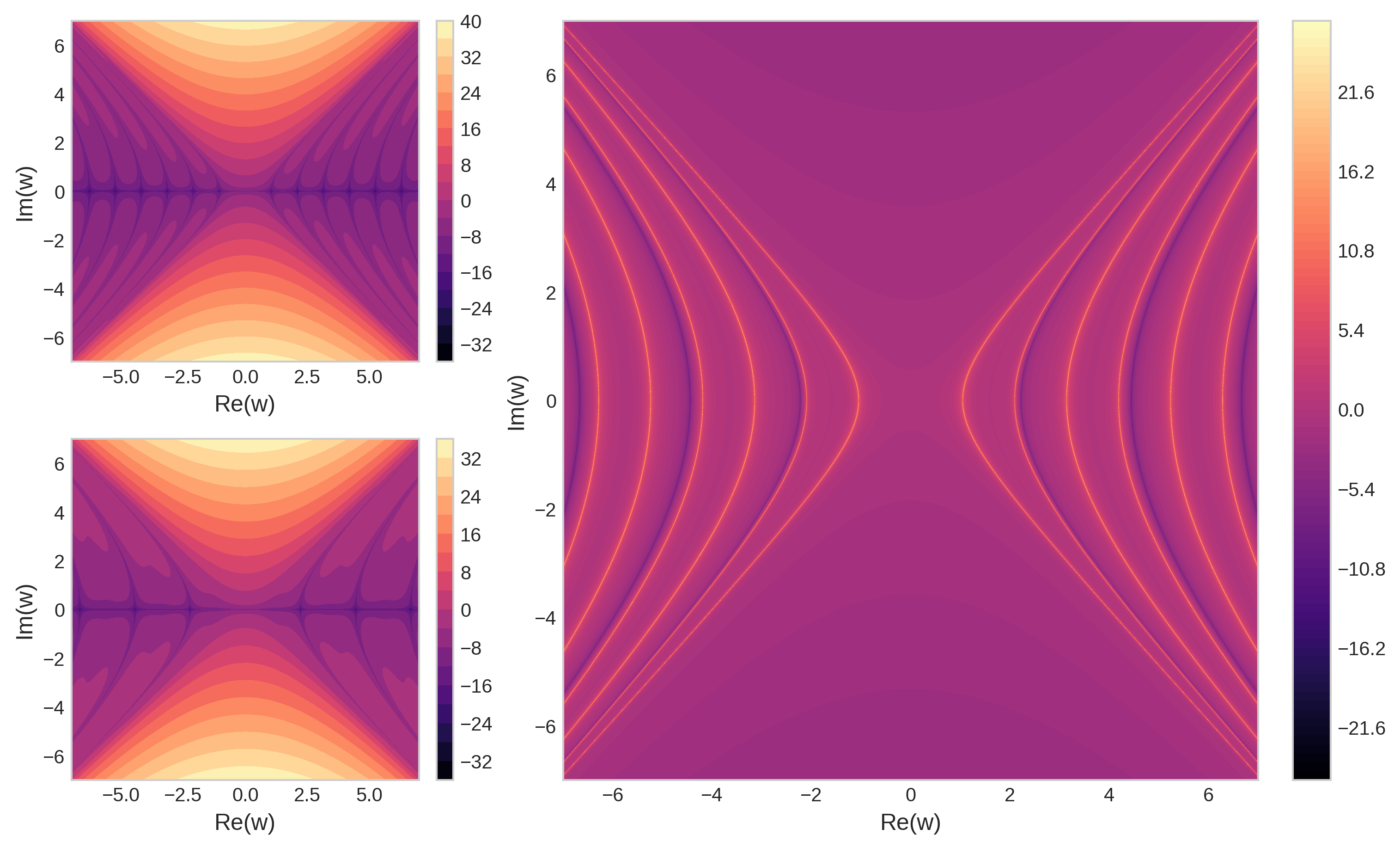
Figure 4: GEM for the first family of three-mode graph states. Top Left: Logarithm of the GEM for the fully connected graph. Bottom Left: Logarithm of the GEM for the partially connected graph. Right: Logarithm of the ratio of the partially connected GEM to the fully connected GEM.

Interestingly, we note that the ratio

$$\frac{\text{GEM}_{\text{G}2}}{\text{GEM}_{\text{G}1}}(w) =\frac{3}{8}\frac{\sin^{2}\left(\sqrt{2}\sqrt{\text{Re}(w)^{2}-\text{Im}(w)^{2}}\right)}{\sin^{2}\left(3\sqrt{\text{Re}(w)^{2}-\text{Im}(w)^{2}}\right)}\left(3\cos\left(2\sqrt{2}\sqrt{\text{Re}(w)^{2}-\text{Im}(w)^{2}}\right)+5\right)$$ (73)

$$=\frac{3}{8}\csc^{2}\left(3r\sqrt{\cos(2\phi)}\right)\sin^{2}\left(r\sqrt{\sin(4\phi)\csc(2\phi)}\right)\left(3\cos\left(2r\sqrt{\sin(4\phi)\csc(2\phi)}\right)+5\right)\,.$$

has the following finite limit on the two principal axes in the $w$ complex plane, corresponding to $\phi\to\frac{\pi}{4}+\frac{n\pi}{2}$ with $n\in\{0,1,2,3\}$ (or $r\to 0$):

$$\frac{\text{GEM}_{\text{G}2}}{\text{GEM}_{\text{G}1}}\to\frac{2}{3}\,,$$ (74)

which is precisely the ratio of the number of edges in the two graphs.

Let us mention, without entering into the details, that the above observation concerning how the ratio of GEMs captures information about the connectivity of the underlying graphs actually generalizes to more complicated graph topologies, as can be seen when inspecting the ratio of GEMs for 4-mode graph states (with obvious notations):

$$\frac{\text{GEM}\Big{(}\leavevmode\hbox to8.94pt{\vbox to8.94pt{\text{[drawing]}}}\Big{)}}{\text{GEM}\Big{(}\leavevmode\hbox to8.94pt{\vbox to8.94pt{\text{[drawing]}}}\Big{)}}\to\frac{5}{6}\,, \ \ \ \ \ \frac{\text{GEM}\Big{(}\leavevmode\hbox to8.94pt{\vbox to8.94pt{\text{[drawing]}}}\Big{)}}{\text{GEM}\Big{(}\leavevmode\hbox to8.94pt{\vbox to8.94pt{\text{[drawing]}}}\Big{)}}\to\frac{2}{3}\,,$$ (75)

$$\frac{\text{GEM}\Big{(}\leavevmode\hbox to8.94pt{\vbox to8.94pt{\text{[drawing]}}}\Big{)}}{\text{GEM}\Big{(}\leavevmode\hbox to8.94pt{\vbox to8.94pt{\text{[drawing]}}}\Big{)}}\to\frac{2}{3}\,, \ \ \ \ \ \frac{\text{GEM}\Big{(}\leavevmode\hbox to8.94pt{\vbox to8.94pt{\text{[drawing]}}}\Big{)}}{\text{GEM}\Big{(}\leavevmode\hbox to8.94pt{\vbox to8.94pt{\text{[drawing]}}}\Big{)}}\to\frac{2}{5}\,,$$

$$\frac{\text{GEM}\Big{(}\leavevmode\hbox to8.94pt{\vbox to8.94pt{\text{[drawing]}}}\Big{)}}{\text{GEM}\Big{(}\leavevmode\hbox to8.94pt{\vbox to8.94pt{\text{[drawing]}}}\Big{)}}\to\frac{1}{2}\,, \ \ \ \ \ \frac{\text{GEM}\Big{(}\leavevmode\hbox to8.94pt{\vbox to8.94pt{\text{[drawing]}}}\Big{)}}{\text{GEM}\Big{(}\leavevmode\hbox to8.94pt{\vbox to8.94pt{\text{[drawing]}}}\Big{)}}\to\frac{4}{5}\,.$$

Second family:

Given that, as we saw, the real part of the coupling to not play an important role regarding the generation of entanglement in the sense of our measure, and in order to study the effect of the ratio of the communication strength between the vertices of the graph, let us now set $\text{Re}(A_{\mu\nu})=0$ and consider again the two graph topologies discussed above. For the fully connected graph (G1) we set $A_{13}=1$, and for both graphs we set $A_{12}=ix$ and $A_{23}=iy$, cf. fig. 5.

Inspecting the ratio of the GEMs, we observe that asymptotically at large times (or large strength of the couplings), the ratio tends to $1$. Namely provided enough time has passed, the two states reach the same level of entanglement in the sense of our measure. However, we observe that the more balanced the strength $x$ and $y$ of the two edges are, the faster the two states reach a similar level of GEM entanglement.

Figure 5: Second family of three-mode graph states, with imaginary unequal couplings.

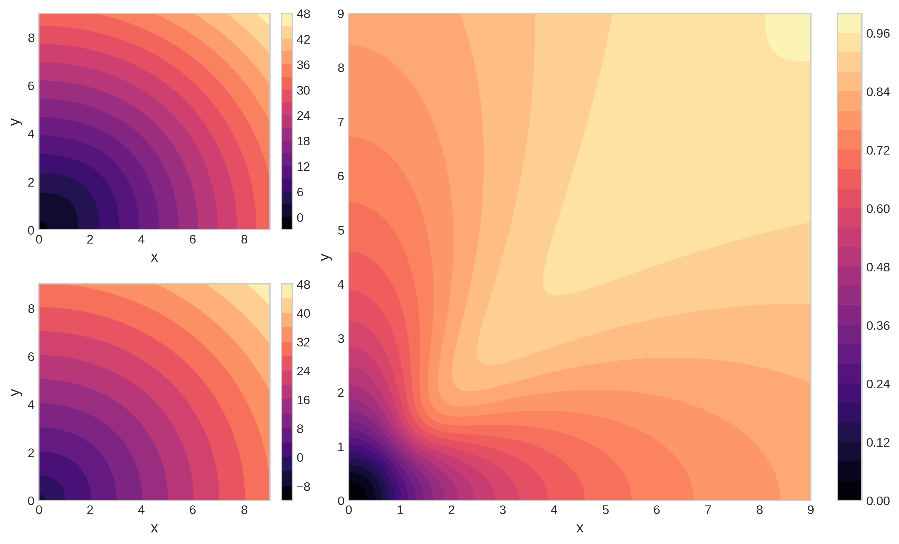
Figure 6: GEM for the second family of three-mode graph states. Top Left: Logarithm of the GEM for the fully connected graph. Bottom Left: Logarithm of the GEM for the partially connected graph. Right: Ratio of the partially connected GEM to the fully connected GEM.

III.2 Free scalar field

Instead of considering systems with slightly more degrees of freedom, let us directly study the case of a very large number of bosonic modes. We therefore consider in this section a massive real Klein-Gordon field in $(1+1)$ dimensions (we set the speed of light $c$ to unity). We refer the reader to App. B for details concerning this example.

We compactify the spatial dimension on a circle $S^{1}$ of radius $R$. The Lagrangian density of the system reads (we use the signature $(+,-)$ for the flat Lorentzian metric):

$$\mathcal{L}=\frac{1}{2}\Big{(}\partial_{\mu}\phi\partial^{\mu}\phi-m^{2}\phi^{2}\Big{)}\,.$$ (76)

Introducing, as usual, the conjugate momentum to the field

$$\Pi=\frac{\partial\mathcal{L}}{\partial(\partial_{0}\phi)}=\partial_{0}\phi\,,$$ (77)

the Hamiltonian density reads:

$$\mathcal{H}=\frac{1}{2}\Big{(}\Pi^{2}+(\bm{\nabla}\phi)^{2}+m^{2}\phi^{2}\Big{)}\,.$$ (78)

We discretize the theory and solely consider the values of the field and its conjugate momentum on a lattice $\mathbb{Z}_{N}\subset S^{1}$ composed of $N=2n+1$ points $\{x_{\mu}\}_{\mu=1}^{N}$ separated by a distance $\delta=2\pi R/N$. The Hamiltonian of the discretized theory then reads ($Q_{N+1}\stackrel{{\scriptstyle\text{def}}}{{=}}Q_{1}\,,P_{N+1}\stackrel{{\scriptstyle\text{def}}}{{=}}P_{1}$)

$$\hat{H}=\sum_{\mu=1}^{N}\left(\frac{\delta}{2}\hat{P}_{\mu}^{2}+\frac{1}{2\delta}\omega^{2}\hat{Q}_{\mu}^{2}-\frac{1}{\delta^{3}}\hat{Q}_{\mu}\hat{Q}_{\mu+1}\right)\,,$$ (79)

with

$$\hat{Q}_{\mu}=\phi(x_{\mu})\delta\,,\ \ \ \ \ \hat{P}_{\mu}=\Pi(x_{\mu})\,.$$ (80)

and where we defined the effective frequency:

$$\omega\stackrel{{\scriptstyle\text{def}}}{{=}}\sqrt{m^{2}+\frac{2}{\delta^{2}}}\,.$$ (81)

By translation invariance, the Hamiltonian can be diagonalized by discrete Fourier transform ($0\leq k\leq N-1$):

$$\hat{q}_{k}=\frac{1}{\sqrt{N}}\sum_{\mu=1}^{N}e^{\frac{2i\pi k\mu}{N}}\hat{Q}_{\mu}\,,\ \ \ \ \ \hat{p}_{k}=\frac{1}{\sqrt{N}}\sum_{\mu=1}^{N}e^{-\frac{2i\pi k\mu}{N}}\hat{P}_{\mu}\,.$$ (82)

We further separate the complex modes into real and imaginary parts by defining for all $1\leq k\leq n$

$$\hat{q}_{\textsc{r},k}=\frac{\hat{q}_{k}+\hat{q}_{-k}}{\sqrt{2}}\,,\ \ \ \ \hat{p}_{\textsc{r},k}=\frac{\hat{p}_{k}+\hat{p}_{-k}}{\sqrt{2}}\,,$$ (83)

$$\hat{q}_{\textsc{i},k}=\frac{\hat{q}_{k}-\hat{q}_{-k}}{i\sqrt{2}}\,,\ \ \ \ \ \hat{p}_{\textsc{i},k}=i\,\frac{\hat{p}_{k}-\hat{p}_{-k}}{\sqrt{2}}\,,$$

in terms of which the Hamiltonian is expressed as a collection of uncoupled harmonic oscillators:

$$H =\frac{\delta}{2}\,\hat{p}_{0}^{2}+\frac{m^{2}}{2\delta}\,\hat{q}_{0}^{2}+$$ (84)

$$+\sum_{k=1}^{n}\left(\frac{\delta}{2}\,\hat{p}_{\textsc{r},k}^{2}+\frac{\omega_{k}^{2}}{2\delta}\,\hat{q}_{\textsc{r},k}^{2}+\frac{\delta}{2}\,\hat{p}_{\textsc{i},k}^{2}+\frac{\omega_{k}^{2}}{2\delta}\,\hat{q}_{\textsc{i},k}^{2}\right)\,,$$

with the familiar dispersion relation:

$$\omega_{k}=\sqrt{m^{2}+\frac{4}{\delta^{2}}\sin^{2}\left(\frac{\pi k}{N}\right)}\,.$$ (85)

We define the dimensionless creation (and annihilation) operators by

$$\hat{a}_{\mu} =\frac{1}{\sqrt{2}}\left(\sqrt{\frac{\omega}{\delta}}\,\hat{Q}_{\mu}+i\sqrt{\frac{\delta}{\omega}}\,\hat{P}_{\mu}\right)\,,\ \mu=1,\dots,N\,,$$

$$\hat{b}_{0} =\frac{1}{\sqrt{2}}\left(\sqrt{\frac{m}{\delta}}\,\hat{q}_{0}+i\sqrt{\frac{\delta}{m}}\,\hat{p}_{0}\right)\,,$$ (86)

$$\hat{b}_{\textsc{r},k} =\frac{1}{\sqrt{2}}\left(\sqrt{\frac{\omega_{k}}{\delta}}\,\hat{q}_{\textsc{r},k}+i\sqrt{\frac{\delta}{\omega_{k}}}\,\hat{p}_{\textsc{r},k}\right)\,,\ k=1,\dots,n\,.$$

$$\hat{b}_{\textsc{i},k} =\frac{1}{\sqrt{2}}\left(\sqrt{\frac{\omega_{k}}{\delta}}\,\ \hat{q}_{\textsc{i},k}+i\sqrt{\frac{\delta}{\omega_{k}}}\,\hat{p}_{\textsc{i},k}\right)\,,\ \ \,k=1,\dots,n\,.$$

Following the conventions of [72], we gather them into vectors

$$\hat{\bm{\alpha}} =\left(\hat{a}_{1},\dots,\hat{a}_{N},\hat{a}_{1}^{\dagger},\dots,\hat{a}_{N}^{\dagger}\right)^{\textsc{t}}\,,$$ (87)

$$\hat{\bm{\beta}} =\left(b_{0},b_{\textsc{r},k},b_{\textsc{i},k},b_{0}^{\dagger},b_{\textsc{r},k}^{\dagger},b_{\textsc{i},k}^{\dagger}\right)^{\textsc{t}}\,,$$

such that one then has $\hat{\bm{\beta}}=T\hat{\bm{\alpha}}$ with the Bogoliubov transformation matrix:

$$T=\left[\begin{array}[]{c|c}X^{*}&-Y^{*}\\ \hline\cr-Y&X\end{array}\right]\,,$$ (88)

with the matrices $X$ and $Y$ given by:

$$X=\frac{1}{\sqrt{N}} \left[\begin{array}[]{c}\frac{1}{2}\left(\sqrt{\frac{m}{\omega}}+\sqrt{\frac{\omega}{m}}\right)\bm{1}_{1\times N}\\ \left(\frac{1}{\sqrt{2}}\cos\left(\frac{2\pi ka}{N}\right)\left(\sqrt{\frac{\omega_{k}}{\omega}}+\sqrt{\frac{\omega}{\omega_{k}}}\right)\right)_{k,a}\\ \left(\frac{1}{\sqrt{2}}\sin\left(\frac{2\pi ka}{N}\right)\left(-\sqrt{\frac{\omega_{k}}{\omega}}+\sqrt{\frac{\omega}{\omega_{k}}}\right)\right)_{k,a}\end{array}\right]\,,$$ (89)

$$Y=-\frac{1}{\sqrt{N}} \left[\begin{array}[]{c}\frac{1}{2}\left(\sqrt{\frac{m}{\omega}}-\sqrt{\frac{\omega}{m}}\right)\bm{1}_{1\times N}\\ \left(\frac{1}{\sqrt{2}}\cos\left(\frac{2\pi ka}{N}\right)\left(\sqrt{\frac{\omega_{k}}{\omega}}-\sqrt{\frac{\omega}{\omega_{k}}}\right)\right)_{k,a}\\ \left(\frac{1}{\sqrt{2}}\sin\left(\frac{2\pi ka}{N}\right)\left(-\sqrt{\frac{\omega_{k}}{\omega}}-\sqrt{\frac{\omega}{\omega_{k}}}\right)\right)_{k,a}\end{array}\right]\,.$$

From the expressions above, one can easily check that the matrix $T$ does define a genuine symplectic transformation, namely that $T\in\text{Sp}(2N,\mathbb{R})$:

$$XX^{\dagger}-YY^{\dagger} =\mathbb{1}\,,\ \ \ \ \ XY^{\textsc{t}}-YX^{\textsc{t}}=0\,,$$ (90)

$$X^{\dagger}X-Y^{\textsc{t}}Y^{*} =\mathbb{1}\,,\ \ \ \ \ X^{\textsc{t}}Y^{*}-Y^{\dagger}X=0\,.$$

The ground state of the system $|\emptyset\rangle$ is a Gaussian state,therefore fully characterized by its correlation matrix.

Using the results reported in Appendix B.2 to express the correlation matrix elements in terms of $X$, $Y$ matrices, the following expression for the determinant of the reduced correlation matrix:

$$\text{det}\left(\Gamma^{(\mu)}\right)=\frac{1}{4}\left(Y^{\dagger}Y+X^{\dagger}X\right)_{\mu\mu}^{2}-\dfrac{\left(Y^{\dagger}X\right)_{\mu\mu}^{2}+\left(X^{\dagger}Y\right)_{\mu\mu}^{2}}{2}\,.$$ (91)

Using the expression of the matrices $X$ and $Y$, one can compute this determinant very explicitly. After the dust settles down, we obtain:

$$\text{det}\left(\Gamma^{(\mu)}\right)=\frac{1}{4N^{2}}\left[1+2\sum_{k=1}^{n}\left(\frac{m}{\omega_{k}}+\frac{\omega_{k}}{m}\right)+4\sum_{k,k^{\prime}}\frac{\omega_{k}}{\omega_{k^{\prime}}}\right]\,.$$ (92)

The GEM of the ground state of the QFT then reads:

$$\text{GEM}[|\emptyset\rangle]=\frac{1}{32N}\left[1+2\sum_{k=1}^{\frac{N-1}{2}}\left(\frac{m}{\omega_{k}}+\frac{\omega_{k}}{m}\right)+4\sum_{k=1}^{\frac{N-1}{2}}\sum_{k^{\prime}=1}^{\frac{N-1}{2}}\frac{\omega_{k}}{\omega_{k^{\prime}}}\right]-\frac{N}{32}\,.$$ (93)

In the large mass limit, the GEM vanishes

$$\text{GEM}[|\emptyset\rangle]\underset{m\to\infty}{\rightarrow}0\,,$$ (94)

which is consistent with the fact that in the infinite mass limit, the coupling between neighbouring sites becomes subleading, and therefore quantum correlations are not present in the vacuum state, which simply corresponds to the (separable) tensor product of Fock vacua. Instead, in the limit of small mass parameter, the GEM diverges as the inverse of the mass:

$$\text{GEM}[|\emptyset\rangle]\underset{m\to 0}{\sim}\frac{1}{32\pi Rm}\cot\left(\frac{\pi}{2N}\right)\,.$$ (95)

This is also consistent with the fact that the continuum theory becomes conformal in that limit because of the absence of any typical length scale.

Another very interesting limit is the continuum limit, in which the regularization parameter $N=2n+1$ goes to infinity for fixed mass $m$ and the radius of space $R$. In App. (B.3), we derive the asymptotic behavior of the GEM at large $n$. We obtain the following behavior:

$$\text{GEM}[|\emptyset\rangle]\underset{n\to\infty}{\sim}\kappa^{(1)}_{p}(\tau)+\kappa^{(2)}_{p}(\tau)\log n+\kappa^{(3)}_{p}(\tau)\,n+\kappa^{(4)}_{p}(\tau)\,n\log n+\mathcal{O}(n^{-1})\,,$$ (96)

where $\tau\stackrel{{\scriptstyle\text{def}}}{{=}}mR$, and where the parameter $p\in\mathbb{N}$, the ’Bernoulli cutoff’, is explained in App. (B.3). Let us simply say that, in principle, the larger the cutoff, the more precise the value of the coefficients $\kappa^{(\ell)}_{p}(\tau)$, but that in practice the a priori very crude approximation $p=0$ already gives a very good estimate. Therefore we observe that GEM diverges in the limit of an infinitely dense lattice in a controlled way. A few comments should be made at this point. First, note that the coefficients $\kappa^{(\ell)}_{p}$ depend on the mass and radius only through their dimensionless combination $\tau$. Second, the coefficients $\kappa^{(2)}_{p}$ and $\kappa^{(4)}_{p}$ turn out to depend neither on the Bernoulli cutoff $p$, nor on the modulus $\tau$. They are given by

$$\kappa^{(2)}_{p}(\tau)=\frac{1}{16\pi}\,,\ \ \ \ \ \ \kappa^{(4)}_{p}(\tau)=\frac{1}{4\pi^{2}}\,.$$ (97)

Euler-Maclaurin expansions generally give good approximations already for small values of the Bernouilly cutoff, and this is indeed what we observe when plugging in some dummy values of the modulus, like $\tau=1$. We observe a stabilization of $\kappa^{(1)}_{p}$ and $\kappa^{(3)}_{p}$ already for $p=3$, and actually $p=0$ is already converged at two decimal figures. For concreteness, we report here the analytical expression of the running coefficients for $p=0$ and $p=1$:

$$\kappa^{(1)}_{p=0}(\tau) =\frac{1}{32\pi}\left(\frac{1}{\sqrt{\tau^{2}+1}}+\frac{1}{\tau}-2\log(\tau)-2\log(\pi)+\log(64)+2\right)\,,$$ (98)

$$\kappa^{(3)}_{p=0}(\tau) =\frac{1}{8\pi^{2}}\left(\frac{1}{\sqrt{\tau^{2}+1}}+\frac{1}{\tau}-2\log(\tau)-2\log(\pi)+\log(64)-\frac{\pi^{2}}{2}\right)\,,$$

$$\kappa^{(1)}_{p=1}(\tau) =\frac{1}{192\pi}\left(\frac{1}{\left(\tau^{2}+1\right)^{3/2}}+\frac{6}{\sqrt{\tau^{2}+1}}+\frac{6}{\tau}-12\log(\tau)-12\log(\pi)+36\log(2)+12\right)\,,$$

$$\kappa^{(3)}_{p=1}(\tau) =\frac{1}{28\pi^{2}}\left(\frac{6\tau^{2}+7}{\left(\tau^{2}+1\right)^{3/2}}+\frac{6}{\tau}-12\log(\tau)-12\log(\pi)+36\log(2)-3\pi^{2}\right)\,.$$

Note that one can directly check that the asymptotic behavior given in eq. (96) is perfectly correct, as can be seen in fig. (7).

Finally, let us say that had we chosen to normalize our expression of the GEM (53) with an extra factor scaling linearly in the size of the system, the above asymptotic behavior would be much simpler, and reduce to the following universal behavior:

$$\text{GEM}[|\emptyset\rangle]\underset{N\to\infty}{\sim}\frac{1}{4\pi^{2}}\,\log N+\mathcal{O}\left(1\right)\,.$$ (99)

Figure 7: Asymptotic fit of the GEM of the free massive Klein-Gordon field, with mass $m=1$ and radius of space $R=1$. We observe a perfect agreement between the exact result given by eq. (93) and the asymptotic behavior predicted by eq. (96).

Outlook

In this work, we have defined the Geometric Gaussian Entanglement Measure, a simple scalar measure of quantum correlations in multimode Gaussian states. The intuition is rooted in the geometric description of the space of Gaussian states [48], leveraging on the Riemannian metric and action of the local Gaussian unitary transformations, in the spirit of what was done for discrete systems in [27]. We then computed the GEM for various natural families of Gaussian states, and observed in particular in the multimode graph case that it naturally captures some topological properties of the underlying graph defining the state.

Let us mention a few natural directions suggested by our definition. Our work naturally extends the results of [27] and can be viewed as a non-compact version of their qubit examples, for which the local algebra of unitaries $\bigoplus_{\mu}\mathfrak{su}(2)\in\mathfrak{su}(2^{M})$ is naturally replaced by the symplectic group $\bigoplus_{\mu}\mathfrak{sp}(2,\mathbb{R})\in\mathfrak{sp}(2M,\mathbb{R})$. From a geometric perspective, this leads to structures reminiscent of the well-known Segre embedding for qubit systems [73], but where the Block sphere $\mathbb{P}^{1}=\text{SU}(2)/\text{U}(1)$ is now replaced by the hyperboloid $\mathbb{H}^{1}=\text{SU}(1,1)/\text{U}(1)$. More generally, the freedom in the choice of the algebra of local transformations allows for a broad generalization of our definitionon. Given an $M$-mode system, one can consider the set of partitions of the set of modes. Given a partition $P$, one associates to it the subalgebra $\bigoplus_{\sigma\in P}\mathfrak{sp}(2|\sigma|,\mathbb{R})\in\mathfrak{sp}(2M,\mathbb{R})$, which can then be chosen a the algebra of ’local’ transformations. The choice made in this paper corresponds then to the choice of the finest partition of the set of modes. The set of partitions is naturally endowed with a partial order corresponding to the level of refinement, and we would expect our generalized GEM to respect that partial order, in the sense that given a state $|\psi\rangle$, its GEM for the coarsest partition (containing solely the whole set of modes) should vanish identically, and should be non-decreasing as the partition is being refined, reaching a maximal value for the finest partition described in this paper. This is left for future investigations.

We saw that the GEM can naturally be expressed in terms of a quadratic Casimir, namely a quadratic element of the center of the universal enveloping algebra. Though slightly deviating from the geometric root of our definition, this observation naturally suggests the possibility of defining a family of entanglement measures in terms of higher-order Casimir operators.

Gaussian states represent an extremely rich class of continuous variable quantum states. However, including even richer families of states beyond Gaussianity is of critical importance. One possibility consists in considering the stellar representation of quantum states, which provides a neat framework in which non-Gaussianities can be implemented in a very controlled way in terms of the stellar rank [74] (number of zeros of the Husimi Q-function in phase space). Another approach could be to consider families of states generated by the action of higher-order Hamiltonian, as described in [75].

Finally, it will be of great interest to consider the case of bosonic field theories in higher dimension, for instance, a free boson on $\mathbb{R}_{t}\times\Sigma_{g}$, where $\Sigma_{g}$ is a compact Riemann surface of genus $g$. Generally, the coefficients appearing in the asymptotic expansion obtained when switching off the UV cutoff of the theory could capture some invariants of the underlying manifold.

Competing Interests

The Authors declare no Competing Financial or Non-Financial Interests.

Appendix A Moments

We provide here some details about the moments entering in the derivation of the metric tensor in Sec. II.3.

The first moments of the $\mathfrak{sp}(2,\mathbb{R})$ generators are directly given by:

$$M_{1}^{\mu} =\left\langle\phi\left|\frac{q_{\mu}^{2}-p_{\mu}^{2}}{4}\right|\phi\right\rangle =\frac{1}{4}\big{(}\mathcal{C}_{q_{\mu},q_{\mu}}-\mathcal{C}_{p_{\mu},p_{\mu}}\big{)}$$ (100)

$$M_{2}^{\mu} =-\left\langle\phi\left|\frac{p_{\mu}q_{\mu}+q_{\mu}p_{\mu}}{4}\right|\phi\right\rangle =-\frac{1}{4}\big{(}\mathcal{C}_{p_{\mu},q_{\mu}}+\mathcal{C}_{q_{\mu},p_{\mu}}\big{)}$$

$$M_{3}^{\mu} =\left\langle\phi\left|\frac{q_{\mu}^{2}+p_{\mu}^{2}}{4}\right|\phi\right\rangle =\frac{1}{4}\big{(}\mathcal{C}_{q_{\mu},q_{\mu}}+\mathcal{C}_{p_{\mu},p_{\mu}}\big{)}$$

For the second moments, application of Wick’s theorem gives:

$$M_{11}^{\mu\nu} =\frac{1}{16}\left(2\mathcal{C}_{p_{\mu},p_{\nu}}^{2}-2\mathcal{C}_{p_{\mu},q_{\nu}}^{2}-2\mathcal{C}_{q_{\mu},p_{\nu}}^{2}+\left(\mathcal{C}_{p_{\mu},p_{\mu}}-\mathcal{C}_{q_{\mu},q_{\mu}}\right)\left(\mathcal{C}_{p_{\nu},p_{\nu}}-\mathcal{C}_{q_{\nu},q_{\nu}}\right)+2\mathcal{C}_{q_{\mu},q_{\nu}}^{2}\right)$$ (101)

$$M_{12}^{\mu\nu} =\frac{1}{16}\left(4\mathcal{C}_{p_{\mu},p_{\nu}}\mathcal{C}_{p_{\mu},q_{\nu}}-4\mathcal{C}_{q_{\mu},q_{\nu}}\mathcal{C}_{q_{\mu},p_{\nu}}+\left(\mathcal{C}_{p_{\mu},p_{\mu}}-\mathcal{C}_{q_{\mu},q_{\mu}}\right)\left(\mathcal{C}_{p_{\nu},q_{\nu}}+\mathcal{C}_{q_{\nu},p_{\nu}}\right)\right)$$

$$M_{13}^{\mu\nu} =\frac{1}{16}\left(-2\mathcal{C}_{p_{\mu},p_{\nu}}^{2}-2\mathcal{C}_{p_{\mu},q_{\nu}}^{2}+2\left(\mathcal{C}_{q_{\mu},p_{\nu}}^{2}+\mathcal{C}_{q_{\mu},q_{\nu}}^{2}\right)-\left(\mathcal{C}_{p_{\mu},p_{\mu}}-\mathcal{C}_{q_{\mu},q_{\mu}}\right)\left(\mathcal{C}_{p_{\nu},p_{\nu}}+\mathcal{C}_{q_{\nu},q_{\nu}}\right)\right)$$

$$M_{21}^{\mu\nu} =\frac{1}{16}\left(4\mathcal{C}_{p_{\mu},p_{\nu}}\mathcal{C}_{q_{\mu},p_{\nu}}-4\mathcal{C}_{q_{\mu},q_{\nu}}\mathcal{C}_{p_{\mu},q_{\nu}}+\left(\mathcal{C}_{p_{\mu},q_{\mu}}+\mathcal{C}_{q_{\mu},p_{\mu}}\right)\left(\mathcal{C}_{p_{\nu},p_{\nu}}-\mathcal{C}_{q_{\nu},q_{\nu}}\right)\right)$$

$$M_{22}^{\mu\nu} =\frac{1}{16}\left(4\left(\mathcal{C}_{p_{\mu},q_{\nu}}\mathcal{C}_{q_{\mu},p_{\nu}}+\mathcal{C}_{p_{\mu},p_{\nu}}\mathcal{C}_{q_{\mu},q_{\nu}}\right)+\left(\mathcal{C}_{p_{\mu},q_{\mu}}+\mathcal{C}_{q_{\mu},p_{\mu}}\right)\left(\mathcal{C}_{p_{\nu},q_{\nu}}+\mathcal{C}_{q_{\nu},p_{\nu}}\right)\right)$$

$$M_{23}^{\mu\nu} =\frac{1}{16}\left(-4\left(\mathcal{C}_{p_{\mu},p_{\nu}}\mathcal{C}_{q_{\mu},p_{\nu}}+\mathcal{C}_{q_{\mu},q_{\nu}}\mathcal{C}_{p_{\mu},q_{\nu}}\right)-\left(\mathcal{C}_{p_{\mu},q_{\mu}}+\mathcal{C}_{q_{\mu},p_{\mu}}\right)\left(\mathcal{C}_{p_{\nu},p_{\nu}}+\mathcal{C}_{q_{\nu},q_{\nu}}\right)\right)$$

$$M_{31}^{\mu\nu} =\frac{1}{16}\left(-2\mathcal{C}_{p_{\mu},p_{\nu}}^{2}+2\mathcal{C}_{p_{\mu},q_{\nu}}^{2}-2\mathcal{C}_{q_{\mu},p_{\nu}}^{2}-\left(\mathcal{C}_{p_{\mu},p_{\mu}}+\mathcal{C}_{q_{\mu},q_{\mu}}\right)\left(\mathcal{C}_{p_{\nu},p_{\nu}}-\mathcal{C}_{q_{\nu},q_{\nu}}\right)+2\mathcal{C}_{q_{\mu},q_{\nu}}^{2}\right)$$

$$M_{32}^{\mu\nu} =\frac{1}{16}\left(-4\mathcal{C}_{p_{\mu},p_{\nu}}\mathcal{C}_{p_{\mu},q_{\nu}}-4\mathcal{C}_{q_{\mu},q_{\nu}}\mathcal{C}_{q_{\mu},p_{\nu}}-\left(\mathcal{C}_{p_{\mu},p_{\mu}}+\mathcal{C}_{q_{\mu},q_{\mu}}\right)\left(\mathcal{C}_{p_{\nu},q_{\nu}}+\mathcal{C}_{q_{\nu},p_{\nu}}\right)\right)$$

$$M_{33}^{\mu\nu} =\frac{1}{16}\left(2\mathcal{C}_{p_{\mu},p_{\nu}}^{2}+2\mathcal{C}_{p_{\mu},q_{\nu}}^{2}+2\left(\mathcal{C}_{q_{\mu},p_{\nu}}^{2}+\mathcal{C}_{q_{\mu},q_{\nu}}^{2}\right)+\left(\mathcal{C}_{p_{\mu},p_{\mu}}+\mathcal{C}_{q_{\mu},q_{\mu}}\right)\left(\mathcal{C}_{p_{\nu},p_{\nu}}+\mathcal{C}_{q_{\nu},q_{\nu}}\right)\right)$$

Appendix B Free scalar field

In this appendix, we provide details concerning the derivation of the GEM of a free massive.

B.1 Derivation of the Bogoliubov transform

As explained in Sec. III.2, the starting Hamiltonian reads:

$$H=\sum_{\mu=1}^{N}\left(\frac{\delta}{2}P_{\mu}^{2}+\frac{m^{2}}{2\delta}Q_{\mu}^{2}+\frac{1}{2\delta^{3}}\left(Q_{\mu}-Q_{\mu+1}\right)^{2}\right)=\sum_{\mu=1}^{N}\left(\frac{\delta}{2}P_{\mu}^{2}+\frac{1}{2\delta}\omega^{2}Q_{\mu}^{2}-\frac{1}{\delta^{3}}Q_{\mu}Q_{\mu+1}\right)\,.$$ (102)

where we defined the effective frequency:

$$\omega\stackrel{{\scriptstyle\text{def}}}{{=}}\sqrt{m^{2}+\frac{2}{\delta^{2}}}\,.$$ (103)

The Hamiltonian can be diagonalized by discrete Fourier transform ($0\leq k\leq N-1$)

$$q_{k}=\frac{1}{\sqrt{N}}\sum_{\mu=1}^{N}e^{\frac{2i\pi k\mu}{N}}Q_{\mu}\,,\ \ \ \ \ p_{k}=\frac{1}{\sqrt{N}}\sum_{\mu=1}^{N}e^{-\frac{2i\pi k\mu}{N}}P_{\mu}\,.$$ (104)

We further define for all $1\leq k\leq\frac{N-1}{2}$

$$q_{\textsc{r},k}=\frac{q_{k}+q_{-k}}{\sqrt{2}}\,,\ \ \ \ \ p_{\textsc{r},k}=\frac{p_{k}+p_{-k}}{\sqrt{2}}\,,\ \ \ \ \ q_{\textsc{i},k}=\frac{q_{k}-q_{-k}}{i\sqrt{2}}\,,\ \ \ \ \ p_{\textsc{i},k}=i\frac{p_{k}-p_{-k}}{\sqrt{2}}\,,$$ (105)

in terms of which the Hamiltonian reads

$$H=\frac{\delta}{2}\,p_{0}^{2}+\frac{m^{2}}{2\delta}\,q_{0}^{2}+\sum_{k=1}^{\frac{N-1}{2}}\left(\frac{\delta}{2}\,p_{\textsc{r},k}^{2}+\frac{\omega_{k}^{2}}{2\delta}\,q_{\textsc{r},k}^{2}+\frac{\delta}{2}\,p_{\textsc{i},k}^{2}+\frac{\omega_{k}^{2}}{2\delta}\,q_{\textsc{i},k}^{2}\right)\,,$$ (106)

with

$$\omega_{k}=\sqrt{m^{2}+\frac{4}{\delta^{2}}\sin^{2}\left(\frac{\pi k}{N}\right)}\,.$$ (107)

The canonical change of variable we performed in terms of positions and momenta is therefore

$$q_{0} =\frac{1}{\sqrt{N}}\sum_{\mu=1}^{N}Q_{\mu}\,, \ \ \ \ \ \ p_{0}=\frac{1}{\sqrt{N}}\sum_{\mu=1}^{N}P_{\mu}\,,$$ (108)

$$q_{\textsc{r},k} =\sqrt{\frac{2}{N}}\sum_{\mu=1}^{N}\cos\left(\frac{2\pi k\mu}{N}\right)Q_{\mu}\,, \ \ \ \ p_{\textsc{r},k}=\sqrt{\frac{2}{N}}\sum_{\mu=1}^{N}\cos\left(\frac{2\pi k\mu}{N}\right)P_{\mu}\,,$$

$$q_{\textsc{i},k} =\sqrt{\frac{2}{N}}\sum_{\mu=1}^{N}\sin\left(\frac{2\pi k\mu}{N}\right)Q_{\mu}\,, \ \ \ \ p_{\textsc{i},k}=\sqrt{\frac{2}{N}}\sum_{\mu=1}^{N}\sin\left(\frac{2\pi k\mu}{N}\right)P_{\mu}\,.$$

We define the dimensionless creation (and annihilation) operators by

$$a_{\mu}=\frac{1}{\sqrt{2}}\left(\sqrt{\frac{\omega}{\delta}}Q_{\mu}+i\sqrt{\frac{\delta}{\omega}}P_{\mu}\right)\,,\ \ b_{0}=\frac{1}{\sqrt{2}}\left(\sqrt{\frac{m}{\delta}}q_{0}+i\sqrt{\frac{\delta}{m}}p_{0}\right)\,,\ \ b_{\textsc{r}/\textsc{i},k}=\frac{1}{\sqrt{2}}\left(\sqrt{\frac{\omega_{k}}{\delta}}q_{\textsc{r}/\textsc{i},k}+i\sqrt{\frac{\delta}{\omega_{k}}}p_{\textsc{r},\textsc{i},k}\right)\,,$$ (109)

in terms of which

$$H =\frac{\omega}{2}\sum_{\mu=1}^{N}\left(a_{\mu}^{\dagger}a_{\mu}+a_{\mu}a_{\mu}^{\dagger}-\frac{1}{\delta^{2}\omega^{2}}\left(a_{\mu}+a_{\mu}^{\dagger}\right)\left(a_{\mu+1}+a_{\mu+1}^{\dagger}\right)\right)$$ (110)

$$=\frac{m}{2}\left(b_{0}^{\dagger}b_{0}+b_{0}b_{0}^{\dagger}\right)+\sum_{k=1}^{\frac{N-1}{2}}\frac{\omega_{k}}{2}\left(b_{\textsc{r},k}^{\dagger}b_{\textsc{r},k}+b_{\textsc{r},k}b_{\textsc{r},k}^{\dagger}+b_{\textsc{i},k}^{\dagger}b_{\textsc{i},k}+b_{\textsc{i},k}b_{\textsc{i},k}^{\dagger}\right)\,.$$

In the creation/annihilation basis, the canonical transformation (108) reads:

$$b_{0} =\frac{1}{2}\frac{1}{\sqrt{N}}\sum_{\mu=1}^{N}\left[\left(\sqrt{\frac{m}{\omega}}+\sqrt{\frac{\omega}{m}}\right)a_{\mu}+\left(\sqrt{\frac{m}{\omega}}-\sqrt{\frac{\omega}{m}}\right)a_{\mu}^{\dagger}\right]\,,$$ (111)

$$b_{0}^{\dagger} =\frac{1}{2}\frac{1}{\sqrt{N}}\sum_{\mu=1}^{N}\left[\left(\sqrt{\frac{m}{\omega}}-\sqrt{\frac{\omega}{m}}\right)a_{\mu}+\left(\sqrt{\frac{m}{\omega}}+\sqrt{\frac{\omega}{m}}\right)a_{\mu}^{\dagger}\right]\,,$$

$$b_{\textsc{r},k} =\frac{1}{2}\sqrt{\frac{2}{N}}\sum_{\mu=1}^{N}\cos\left(\frac{2\pi k\mu}{N}\right)\left[\left(\sqrt{\frac{\omega_{k}}{\omega}}+\sqrt{\frac{\omega}{\omega_{k}}}\right)a_{\mu}+\left(\sqrt{\frac{\omega_{k}}{\omega}}-\sqrt{\frac{\omega}{\omega_{k}}}\right)a_{\mu}^{\dagger}\right]\,,$$

$$b_{\textsc{r},k}^{\dagger} =\frac{1}{2}\sqrt{\frac{2}{N}}\sum_{\mu=1}^{N}\cos\left(\frac{2\pi k\mu}{N}\right)\left[\left(\sqrt{\frac{\omega_{k}}{\omega}}-\sqrt{\frac{\omega}{\omega_{k}}}\right)a_{\mu}+\left(\sqrt{\frac{\omega_{k}}{\omega}}+\sqrt{\frac{\omega}{\omega_{k}}}\right)a_{\mu}^{\dagger}\right]\,,$$

$$b_{\textsc{i},k} =\frac{1}{2}\sqrt{\frac{2}{N}}\sum_{\mu=1}^{N}\sin\left(\frac{2\pi k\mu}{N}\right)\left[\left(\sqrt{\frac{\omega_{k}}{\omega}}+\sqrt{\frac{\omega}{\omega_{k}}}\right)a_{\mu}+\left(-\sqrt{\frac{\omega_{k}}{\omega}}-\sqrt{\frac{\omega}{\omega_{k}}}\right)a_{\mu}^{\dagger}\right]\,,$$

$$b_{\textsc{i},k}^{\dagger} =\frac{1}{2}\sqrt{\frac{2}{N}}\sum_{\mu=1}^{N}\sin\left(\frac{2\pi k\mu}{N}\right)\left[\left(\sqrt{\frac{\omega_{k}}{\omega}}-\sqrt{\frac{\omega}{\omega_{k}}}\right)a_{\mu}+\left(-\sqrt{\frac{\omega_{k}}{\omega}}+\sqrt{\frac{\omega}{\omega_{k}}}\right)a_{\mu}^{\dagger}\right]\,,$$

from which one reads out the matrices $X$ and $Y$ defined in eq. (88).

B.2 Derivation of the GEM

The ground state of the system $|\emptyset\rangle$ is a Gaussian state, therefore fully characterized by its correlation matrix. The correlation matrix elements in $(p,q)$-basis and $(a,a^{\dagger})$-basis are related as follows:

$$\Gamma_{q_{\mu},q_{\mu}}=\dfrac{1}{2}\langle\emptyset|(\hat{a}_{\mu}+\hat{a}^{\dagger}_{\mu})(\hat{a}_{\mu}+\hat{a}^{\dagger}_{\mu})|\emptyset\rangle=\dfrac{\Gamma_{a_{\mu}a_{\mu}}+\Gamma_{a_{\mu}^{\dagger}a_{\mu}^{\dagger}}}{2}+\Gamma_{a_{\mu}a_{\mu}^{\dagger}}\,,$$ (112)

$$\Gamma_{p_{\mu},p_{\mu}}=-\dfrac{1}{2}\langle\emptyset|(\hat{a}^{\dagger}_{\mu}-\hat{a}_{\mu})(\hat{a}^{\dagger}_{\mu}-\hat{a}_{\mu})|\emptyset\rangle=\Gamma_{a_{\mu}a_{\mu}^{\dagger}}-\dfrac{\Gamma_{a_{\mu}a_{\mu}}+\Gamma_{a_{\mu}^{\dagger}a_{\mu}^{\dagger}}}{2}\,,$$ (113)

$$\Gamma_{p_{\mu},q_{\mu}}=\dfrac{i}{4}\langle\emptyset|(\hat{a}^{\dagger}_{\mu}-\hat{a}_{\mu})(\hat{a}^{\dagger}_{\mu}-\hat{a}_{\mu})+(\hat{a}^{\dagger}_{\mu}-\hat{a}_{\mu})(\hat{a}^{\dagger}_{\mu}-\hat{a}_{\mu})|\emptyset\rangle=\dfrac{i}{2}\left(\Gamma_{a_{\mu}^{\dagger}a_{\mu}^{\dagger}}-\Gamma_{a_{\mu}a_{\mu}}\right)\,.$$ (114)

It follows that the reduced determiant can be rewritten as

$$\mathrm{det}\left(\Gamma^{(\mu)}\right)=\Gamma_{q_{\mu},q_{\mu}}\Gamma_{p_{\mu},p_{\mu}}-(\Gamma_{q_{\mu},p_{\mu}})^{2}=(\Gamma_{a_{\mu}a_{\mu}^{\dagger}})^{2}-\dfrac{(\Gamma_{a_{\mu}^{\dagger}a_{\mu}^{\dagger}})^{2}+(\Gamma_{a_{\mu}a_{\mu}})^{2}}{2}$$ (115)

Using the inverse of the Bogoliubov matrix

$$T^{-1}=\left[\begin{array}[]{c|c}X^{\textsc{t}}&Y^{\dagger}\\ \hline\cr Y^{\textsc{t}}&X^{\dagger}\end{array}\right]\,,$$ (116)

one can compute the correlation matrix element in $(a,a^{\dagger})$-basis by exploiting the fact that the vacuum state $|\emptyset\rangle$ is annihilated by the pseudo-particle annihilation operators. In the $(a,a^{\dagger})$-basis, one has (with index ordering prescribed by eq. (87)):

$$\Gamma_{AB}=\frac{1}{2}\left\langle\emptyset\left|\left\{\alpha_{A},\alpha_{B}\right\}\right|\emptyset\right\rangle=\frac{1}{2}\left(\mathcal{C}_{A,B}+\mathcal{C}_{B,A}\right)\,,$$ (117)

with the two-point function

$$\mathcal{C}_{A,B}=\left\langle\emptyset\left|\alpha_{A}\alpha_{B}\right|\emptyset\right\rangle\,,$$ (118)

which can be computed In creation/annihilation basis one therefore has

$$\mathcal{C}_{A,B}=\left\langle\emptyset\left|\alpha_{A}\alpha_{B}\right|\emptyset\right\rangle=\sum_{C=1}^{2N}\sum_{D=1}^{2N}\left(T^{-1}\right)_{AC}\left(T^{-1}\right)_{BD}\left\langle\emptyset\left|\beta_{C}\beta_{D}\right|\emptyset\right\rangle=\sum_{c=1}^{N}\left(T^{-1}\right)_{Ac}\left(T^{-1}\right)_{B,c+N}$$ (119)

and therefore

$$\Gamma_{AB}=\frac{1}{2}\sum_{c=1}^{N}\left[\left(T^{-1}\right)_{Ac}\left(T^{-1}\right)_{B,c+N}+\left(T^{-1}\right)_{Bc}\left(T^{-1}\right)_{A,c+N}\right]\,.$$ (120)

One therefore obtains:

$$\text{det}\left(\Gamma^{(\mu)}\right)=\frac{1}{4}\left(Y^{\dagger}Y+X^{\dagger}X\right)_{\mu\mu}^{2}-\dfrac{\left(Y^{\dagger}X\right)_{\mu\mu}^{2}+\left(X^{\dagger}Y\right)_{\mu\mu}^{2}}{2}\,.$$ (121)

Using the expression of the matrices $X$ and $Y$, one can compute this determinant very explicitly. Indeed, one has:

$$(Y^{\dagger}X)_{\mu\mu}=-\frac{1}{2N}\Bigg{\{}\frac{1}{2}\left(\frac{m}{\omega}-\frac{\omega}{m}\right)+\sum_{k=1}^{\frac{N-1}{2}}\left(\frac{\omega_{k}}{\omega}-\frac{\omega}{\omega_{k}}\right)\Bigg{\}}\,,$$ (122)

$$(X^{\dagger}X)_{\mu\mu}=\frac{1}{N}\Bigg{\{}\frac{1}{4}\left(\sqrt{\frac{m}{\omega}}+\sqrt{\frac{\omega}{m}}\right)^{2}+\frac{1}{2}\sum_{k=1}^{\frac{N-1}{2}}\left[\cos^{2}\left(\frac{2\pi k\mu}{N}\right)\left(\sqrt{\frac{\omega_{k}}{\omega}}+\sqrt{\frac{\omega}{\omega_{k}}}\right)^{2}+\sin^{2}\left(\frac{2\pi k\mu}{N}\right)\left(-\sqrt{\frac{\omega_{k}}{\omega}}+\sqrt{\frac{\omega}{\omega_{k}}}\right)^{2}\right]\Bigg{\}}\,,$$

$$(Y^{\dagger}Y)_{\mu\mu}=\frac{1}{N}\Bigg{\{}\frac{1}{4}\left(\sqrt{\frac{m}{\omega}}-\sqrt{\frac{\omega}{m}}\right)^{2}+\frac{1}{2}\sum_{k=1}^{\frac{N-1}{2}}\left[\cos^{2}\left(\frac{2\pi k\mu}{N}\right)\left(\sqrt{\frac{\omega_{k}}{\omega}}-\sqrt{\frac{\omega}{\omega_{k}}}\right)^{2}+\sin^{2}\left(\frac{2\pi k\mu}{N}\right)\left(-\sqrt{\frac{\omega_{k}}{\omega}}-\sqrt{\frac{\omega}{\omega_{k}}}\right)^{2}\right]\Bigg{\}}\,,$$

and therefore

$$(X^{\dagger}X+Y^{\dagger}Y)_{\mu\mu} =\frac{1}{2N}\Bigg{\{}\frac{1}{2}\left(\sqrt{\frac{m}{\omega}}+\sqrt{\frac{\omega}{m}}\right)^{2}+\frac{1}{2}\left(\sqrt{\frac{m}{\omega}}-\sqrt{\frac{\omega}{m}}\right)^{2}+\sum_{k=1}^{\frac{N-1}{2}}\left[\left(\sqrt{\frac{\omega_{k}}{\omega}}+\sqrt{\frac{\omega}{\omega_{k}}}\right)^{2}+\left(\sqrt{\frac{\omega_{k}}{\omega}}-\sqrt{\frac{\omega}{\omega_{k}}}\right)^{2}\right]\Bigg{\}}$$ (123)

$$=\frac{1}{2N}\Bigg{\{}\frac{m}{\omega}+\frac{\omega}{m}+2\sum_{k=1}^{\frac{N-1}{2}}\left[\frac{\omega_{k}}{\omega}+\frac{\omega}{\omega_{k}}\right]\Bigg{\}}\,.$$

Therefore the determinant reads:

$$\text{det}\left(\Gamma^{(\mu)}\right) =\frac{1}{16N^{2}}\Bigg{\{}\frac{m}{\omega}+\frac{\omega}{m}+2\sum_{k=1}^{\frac{N-1}{2}}\left[\frac{\omega_{k}}{\omega}+\frac{\omega}{\omega_{k}}\right]\Bigg{\}}^{2}-\frac{1}{16N^{2}}\Bigg{\{}\frac{m}{\omega}-\frac{\omega}{m}+2\sum_{k=1}^{\frac{N-1}{2}}\left[\frac{\omega_{k}}{\omega}-\frac{\omega}{\omega_{k}}\right]\Bigg{\}}^{2}$$ (124)

$$=\frac{1}{4N^{2}}\left[1+2\sum_{k=1}^{\frac{N-1}{2}}\left(\frac{m}{\omega_{k}}+\frac{\omega_{k}}{m}\right)+4\sum_{k,k^{\prime}}\frac{\omega_{k}}{\omega_{k^{\prime}}}\right]\,.$$

In the limit of small mass parameter

$$\text{GEM}[|\emptyset\rangle] \underset{m\to 0}{\sim}\frac{1}{32N}\left[1+\frac{4}{m\delta}\sum_{k=1}^{\frac{N-1}{2}}\sin\left(\frac{\pi k}{N}\right)+4\sum_{k=1}^{\frac{N-1}{2}}\sum_{k^{\prime}=1}^{\frac{N-1}{2}}\frac{\sin\left(\frac{\pi k}{N}\right)}{\sin\left(\frac{\pi k^{\prime}}{N}\right)}\right]-\frac{N}{32}\underset{m\to 0}{\sim}\frac{1}{32\pi Rm}\cot\left(\frac{\pi}{2N}\right)\,.$$ (125)

B.3 Continuum limit

Let us write the GEM given in eq. (93) as follows (we recall that $N=2n+1$):

$$\text{GEM}[|\emptyset\rangle]=\frac{1}{32(2n+1)}\left(1+\frac{2}{m}A_{n}+2m\bar{A}_{n}+4A_{n}\bar{A}_{n}\right)-\frac{2n+1}{32}\,,$$ (126)

with

$$A_{n}\stackrel{{\scriptstyle\text{def}}}{{=}}\sum_{k=1}^{n}\omega_{k}\,,\ \ \ \ \ \ \ \bar{A}_{n}\stackrel{{\scriptstyle\text{def}}}{{=}}\sum_{k=1}^{n}\omega_{k}^{-1}\,.$$ (127)

with we recall ($R$ being the radius of space)

$$\omega_{k}=\sqrt{m^{2}+\left(\frac{2n+1}{\pi R}\right)^{2}\sin^{2}\left(\frac{\pi k}{2n+1}\right)}\,.$$ (128)

In order to obtain an asymptotic expansion for large $n$ of the two sums $A_{n}$ and $\bar{A}_{n}$, recall the Euler-Maclaurin formula which controls the difference between a sum and its approximating integral:

$$\sum_{k=1}^{n}f(k)=\int_{1}^{n}f(x)\,\text{d}x+\frac{f(1)+f(n)}{2}+\sum_{i=1}^{p}\frac{B_{2i}}{(2i)!}\left(f^{(2i-1)}(n)-f^{(2i-1)}(1)\right)+R_{p,n}\,,$$ (129)

where the Bernoulli numbers are defined by

$$\frac{x}{e^{x}-1}=\sum_{i\geq 0}B_{i}\frac{x^{i}}{i!}\,,$$ (130)

and where the remainder term $R_{p,n}$ is typically small. In our case we fix the integer $p$, that we will call the Bernoulli cutoff, to be small. The integral can be expressed as follows:

$$\int_{1}^{n}f(x)\,\text{d}x=n\int_{0}^{1-\frac{1}{n}}f(ny+1)\,\text{d}y\underset{n\to\infty}{\sim}n\int_{0}^{1}f(ny)\,\text{d}y\,.$$ (131)

Inserting for the function $f$ the functions $g(x)=\omega_{x}$ and $\bar{g}(x)=\omega_{x}^{-1}$, one obtains

$$\int_{0}^{1}g(ny)\,\text{d}y \underset{n\to\infty}{\sim}\frac{2m}{\pi}\,E\left(\frac{\pi}{2}\left|-\left(\frac{2n}{m\pi R}\right)^{2}\right.\right)\,,$$ (132)

$$\int_{0}^{1}\bar{g}(ny)\,\text{d}y \underset{n\to\infty}{\sim}\frac{2}{m\pi}\,F\left(\frac{\pi}{2}\left|-\left(\frac{2n}{m\pi R}\right)^{2}\right.\right)\,,$$

with $E$ and $F$ being the elliptic integrals of second and first kind respectively [76]:

$$E(\phi|m)=\int_{0}^{\phi}\sqrt{1-m\sin^{2}\theta}\,\text{d}\theta\,,\ \ \ \ \ F(\phi|m)=\int_{0}^{\phi}\frac{\,\text{d}\theta}{\sqrt{1-m\sin^{2}\theta}}\,.$$ (133)

Using these results, one can extract the asymptotic behavior of the sums $A_{n}$ and $\bar{A}_{n}$, and then following generic asymptotic behavior of the GEM:

$$\text{GEM}[|\emptyset\rangle]\underset{n\to\infty}{\sim}\kappa^{(1)}_{p}(mR)+\kappa^{(2)}_{p}(mR)\log n+\kappa^{(3)}_{p}(mR)\,n+\kappa^{(4)}_{p}(mR)\,n\log n+\mathcal{O}(n^{-1})\,.$$ (134)

We refer the reader to the main text, Sec. (III.2) for a discussion concerning this result.

Appendix C Metrics

For completeness, we collect here the expression of the metric tensor components for the two-mode graph states, cf. Sec. III.1.1:

$$A =-\frac{1}{16}\sin^{2}(\phi)\sec(2\phi)\sin^{2}\left(2r\sqrt{\cos(2\phi)}\right)\,,$$ (135)

$$B =\frac{1}{16}\left(2-\sin^{2}(\phi)\sec(2\phi)\sin^{2}\left(2r\sqrt{\cos(2\phi)}\right)\right)\,,$$

$$C =\frac{1}{16}\sec(2\phi)\left(\sin^{2}(\phi)\sin^{2}\left(2r\sqrt{\cos(2\phi)}\right)+2\sec(2\phi)\left(\cos^{2}(\phi)-\sin^{2}(\phi)\cos\left(2r\sqrt{\cos(2\phi)}\right)\right)^{2}\right)\,,$$

$$D =-\frac{1}{4}\sin(\phi)\cos(\phi)\sec^{2}(2\phi)\left(\cos^{2}(\phi)-\sin^{2}(\phi)\cos\left(2r\sqrt{\cos(2\phi)}\right)\right)\sin^{2}\left(r\sqrt{\cos(2\phi)}\right)\,,$$

$$E =\frac{1}{4}\sin^{2}(\phi)\sec(2\phi)\sin^{2}\left(r\sqrt{\cos(2\phi)}\right)\left(\sec(2\phi)\sin^{2}\left(r\sqrt{\cos(2\phi)}\right)+1\right)\,.$$

$$(h[\phi])_{(\mu,1)(\nu,1)} =\left[\begin{array}[]{cc}A&B\\ B&A\\ \end{array}\right]\,,\ \ \ \ \ (h[\phi])_{(\mu,1)(\nu,2)}=\left[\begin{array}[]{cc}0&0\\ 0&0\\ \end{array}\right]\,,\ \ \ (h[\phi])_{(\mu,1)(\nu,3)}=\left[\begin{array}[]{cc}0&0\\ 0&0\\ \end{array}\right]\,,$$ (136)

$$(h[\phi])_{(\mu,2)(\nu,2)} =\left[\begin{array}[]{cc}-A&C\\ C&-A\\ \end{array}\right]\,,\ (h[\phi])_{(\mu,2)(\nu,3)}=\left[\begin{array}[]{cc}0&D\\ D&0\\ \end{array}\right]\,,\ (h[\phi])_{(\mu,3)(\nu,3)}=\left[\begin{array}[]{cc}-A&E\\ E&-A\\ \end{array}\right]\,.$$

References

- Arute et al. [2019] F. Arute, K. Arya, R. Babbush, D. Bacon, J. C. Bardin, R. Barends, R. Biswas, S. Boixo, F. G. Brandao, D. A. Buell, et al., Quantum supremacy using a programmable superconducting processor, Nature 574, 505 (2019).
- Wu et al. [2021] Y. Wu, W.-S. Bao, S. Cao, F. Chen, M.-C. Chen, X. Chen, T.-H. Chung, H. Deng, Y. Du, D. Fan, et al., Strong quantum computational advantage using a superconducting quantum processor, Phys. Rev. Lett. 127, 180501 (2021).
- Ma et al. [2021] W.-L. Ma, S. Puri, R. J. Schoelkopf, M. H. Devoret, S. M. Girvin, and L. Jiang, Quantum control of bosonic modes with superconducting circuits, Sci. Bull. 66, 1789 (2021).
- Tebbenjohanns et al. [2021] F. Tebbenjohanns, M. L. Mattana, M. Rossi, M. Frimmer, and L. Novotny, Quantum control of a nanoparticle optically levitated in cryogenic free space, Nature 595, 378 (2021).
- Vidal and Tarrach [1999] G. Vidal and R. Tarrach, Robustness of entanglement, Phys. Rev. A 59, 141 (1999).
- Vidal [2000] G. Vidal, Entanglement monotones, J. Mod. Opt. 47, 355 (2000).
- Vedral et al. [1997a] V. Vedral, M. B. Plenio, M. A. Rippin, and P. L. Knight, Quantifying entanglement, Phys. Rev. Lett. 78, 2275 (1997a).
- Horodecki et al. [2000] M. Horodecki, P. Horodecki, and R. Horodecki, Limits for entanglement measures, Phys. Rev. Lett. 84, 2014 (2000).
- Eisert et al. [2002] J. Eisert, C. Simon, and M. B. Plenio, On the quantification of entanglement in infinite-dimensional quantum systems, Phys. A Math. Gen. 35, 3911 (2002).
- Plenio and Virmani [2007] M. B. Plenio and S. Virmani, An introduction to entanglement measures., Quantum Inf. Comput. 7, 1 (2007).
- Lancien et al. [2016] C. Lancien, S. Di Martino, M. Huber, M. Piani, G. Adesso, and A. Winter, Should entanglement measures be monogamous or faithful?, Phys. Rev. Lett. 117, 060501 (2016).
- Bennett et al. [1996a] C. H. Bennett, D. P. DiVincenzo, J. A. Smolin, and W. K. Wootters, Mixed-state entanglement and quantum error correction, Phys. Rev. A 54, 3824 (1996a).
- Popescu and Rohrlich [1997] S. Popescu and D. Rohrlich, Thermodynamics and the measure of entanglement, Phys. Rev. A 56, R3319 (1997).
- Vidal [1999] G. Vidal, Entanglement of pure states for a single copy, Phys. Rev. Lett. 83, 1046 (1999).
- Wootters [1998] W. K. Wootters, Entanglement of formation of an arbitrary state of two qubits, Phys. Rev. Lett. 80, 2245 (1998).
- Bennett et al. [1996b] C. H. Bennett, G. Brassard, S. Popescu, B. Schumacher, J. A. Smolin, and W. K. Wootters, Purification of noisy entanglement and faithful teleportation via noisy channels, Phys. Rev. Lett. 76, 722 (1996b).
- Horodecki et al. [1998] M. Horodecki, P. Horodecki, and R. Horodecki, Mixed-state entanglement and distillation: Is there a “bound” entanglement in nature?, Phys. Rev. Lett. 80, 5239 (1998).
- Dür et al. [2000] W. Dür, G. Vidal, and J. I. Cirac, Three qubits can be entangled in two inequivalent ways, Phys. Rev. A 62, 062314 (2000).
- Briegel and Raussendorf [2001] H. J. Briegel and R. Raussendorf, Persistent entanglement in arrays of interacting particles, Phys. Rev. Lett. 86, 910 (2001).
- Coffman et al. [2000] V. Coffman, J. Kundu, and W. K. Wootters, Distributed entanglement, Phys. Rev. A 61, 052306 (2000).
- Yu and Song [2005] C.-s. Yu and H.-s. Song, Multipartite entanglement measure, Phys. Rev. A 71, 042331 (2005).
- Eisert and Briegel [2001] J. Eisert and H. J. Briegel, Schmidt measure as a tool for quantifying multiparticle entanglement, Phys. Rev. A 64, 022306 (2001).
- Carvalho et al. [2004] A. R. Carvalho, F. Mintert, and A. Buchleitner, Decoherence and multipartite entanglement, Phys. Rev. Lett. 93, 230501 (2004).
- Pezzé and Smerzi [2009] L. Pezzé and A. Smerzi, Entanglement, nonlinear dynamics, and the heisenberg limit, Phys. Rev. Lett. 102, 100401 (2009).
- Hyllus et al. [2012] P. Hyllus, W. Laskowski, R. Krischek, C. Schwemmer, W. Wieczorek, H. Weinfurter, L. Pezzé, and A. Smerzi, Fisher information and multiparticle entanglement, Phys. Rev. A 85, 022321 (2012).
- Scali and Franzosi [2019] S. Scali and R. Franzosi, Entanglement estimation in non-optimal qubit states, Ann. Phys. 411, 167995 (2019).
- Cocchiarella et al. [2020] D. Cocchiarella, S. Scali, S. Ribisi, B. Nardi, G. Bel-Hadj-Aissa, and R. Franzosi, Entanglement distance for arbitrary m-qudit hybrid systems, Phys. Rev. A 101, 042129 (2020).
- Vesperini et al. [2023] A. Vesperini, G. Bel-Hadj-Aissa, and R. Franzosi, Entanglement and quantum correlation measures for quantum multipartite mixed states, Sci. Rep. 13, 2852 (2023).
- Braunstein and Van Loock [2005] S. L. Braunstein and P. Van Loock, Quantum information with continuous variables, RMP 77, 513 (2005).
- Wang et al. [2007] X.-B. Wang, T. Hiroshima, A. Tomita, and M. Hayashi, Quantum information with gaussian states, Phys. Rep. 448, 1 (2007).
- Weedbrook et al. [2012] C. Weedbrook, S. Pirandola, R. García-Patrón, N. J. Cerf, T. C. Ralph, J. H. Shapiro, and S. Lloyd, Gaussian quantum information, RMP 84, 621 (2012).
- Adesso et al. [2014] G. Adesso, S. Ragy, and A. R. Lee, Continuous variable quantum information: Gaussian states and beyond, Open Syst. Inf. Dyn. 21, 1440001 (2014).
- Wald [1994] R. M. Wald, Quantum field theory in curved spacetime and black hole thermodynamics (University of Chicago press, Chicago, US, 1994).
- Parker and Toms [2009] L. Parker and D. Toms, Quantum field theory in curved spacetime: quantized fields and gravity (Cambridge university press, Cambridge, UK, 2009).
- Umezawa et al. [1982] H. Umezawa, H. Matsumoto, and M. Tachiki, Thermo field dynamics and condensed states (North Holland, Amsterdam, NL, 1982).
- Blasone et al. [2011] M. Blasone, P. Jizba, and G. Vitiello, Quantum Field Theory and its macroscopic manifestations: Boson condensation, ordered patterns, and topological defects (World Scientific, London, UK, 2011).
- Berezin [2012] F. Berezin, The method of second quantization, Vol. 24 (Elsevier, Orlando, US, 2012).
- Guaita et al. [2019] T. Guaita, L. Hackl, T. Shi, C. Hubig, E. Demler, and J. I. Cirac, Gaussian time-dependent variational principle for the bose-hubbard model, Phys. Rev. B 100, 094529 (2019).
- Windt et al. [2021] B. Windt, A. Jahn, J. Eisert, and L. Hackl, Local optimization on pure gaussian state manifolds, SciPost Phys. 10, 066 (2021).
- Cerezo et al. [2021] M. Cerezo, A. Arrasmith, R. Babbush, S. C. Benjamin, S. Endo, K. Fujii, J. R. McClean, K. Mitarai, X. Yuan, L. Cincio, et al., Variational quantum algorithms, Nat. Rev. Phys. 3, 625 (2021).
- Chen [2005] X.-y. Chen, Gaussian relative entropy of entanglement, Phys. Rev. A 71, 062320 (2005).
- De Palma and Hackl [2022] G. De Palma and L. Hackl, Linear growth of the entanglement entropy for quadratic hamiltonians and arbitrary initial states, SciPost Phys. 12, 021 (2022).
- Adesso and Illuminati [2005] G. Adesso and F. Illuminati, Gaussian measures of entanglement versus negativities: Ordering of two-mode gaussian states, Phys. Rev. A 72, 032334 (2005).
- Adesso et al. [2006] G. Adesso, A. Serafini, and F. Illuminati, Multipartite entanglement in three-mode gaussian states of continuous-variable systems: Quantification, sharing structure, and decoherence, Phys. Rev. A 73, 032345 (2006).
- Tserkis and Ralph [2017] S. Tserkis and T. C. Ralph, Quantifying entanglement in two-mode gaussian states, Phys. Rev. A 96, 062338 (2017).
- Hackl and Myers [2018] L. Hackl and R. C. Myers, Circuit complexity for free fermions, J. High Energy Phys. 2018 (7), 1.
- Chapman et al. [2019] S. Chapman, J. Eisert, L. Hackl, M. P. Heller, R. Jefferson, H. Marrochio, and R. Myers, Complexity and entanglement for thermofield double states, SciPost Phys. 6, 034 (2019).
- Hackl et al. [2020] L. Hackl, T. Guaita, T. Shi, J. Haegeman, E. Demler, and I. Cirac, Geometry of variational methods: dynamics of closed quantum systems, SciPost Phys. 9, 048 (2020).
- Hackl and Bianchi [2021] L. Hackl and E. Bianchi, Bosonic and fermionic gaussian states from kähler structures, SciPost Phys. Core 4, 025 (2021).
- Nishioka [2018] T. Nishioka, Entanglement entropy: Holography and renormalization group, Rev. Mod. Phys. 90, 035007 (2018).
- Calabrese and Cardy [2009] P. Calabrese and J. Cardy, Entanglement entropy and conformal field theory, J. Phys. A Math. Theor. 42, 504005 (2009).
- Casini and Huerta [2009] H. Casini and M. Huerta, Entanglement entropy in free quantum field theory, J. Phys. A Math. Theor. 42, 504007 (2009).
- Witten [2018] E. Witten, Aps medal for exceptional achievement in research: Invited article on entanglement properties of quantum field theory, Rev. Mod. Phys. 90, 045003 (2018).
- Hollands and Sanders [2017] S. Hollands and K. Sanders, Entanglement measures and their properties in quantum field theory, arXiv:1702.04924 (2017).
- Rangamani and Takayanagi [2017] M. Rangamani and T. Takayanagi, Holographic Entanglement Entropy, Vol. 931 (Springer, Cham, CH, 2017) arXiv:1609.01287 [hep-th] .
- Tóth [2012] G. Tóth, Multipartite entanglement and high-precision metrology, Phys. Rev. A 85, 022322 (2012).
- Pezzè and Smerzi [2014] L. Pezzè and A. Smerzi, Quantum theory of phase estimation, in Atom Interferometry (IOS Press, 2014) pp. 691–741.
- Hauke et al. [2016] P. Hauke, M. Heyl, L. Tagliacozzo, and P. Zoller, Measuring multipartite entanglement through dynamic susceptibilities, Nat. Phys. 12, 778 (2016).
- Rajabpour [2017] M. Rajabpour, Multipartite entanglement and quantum fisher information in conformal field theories, Phys. Rev. D 96, 126007 (2017).
- Paris et al. [2003] M. G. Paris, F. Illuminati, A. Serafini, and S. De Siena, Purity of gaussian states: Measurement schemes and time evolution in noisy channels, Phys. Rev. A 68, 012314 (2003).
- Facchi et al. [2008] P. Facchi, G. Florio, G. Parisi, and S. Pascazio, Maximally multipartite entangled states, Phys. Rev. A 77, 060304 (2008).
- Facchi et al. [2009] P. Facchi, G. Florio, C. Lupo, S. Mancini, and S. Pascazio, Gaussian maximally multipartite-entangled states, Phys. Rev. A 80, 062311 (2009).
- Vedral et al. [1997b] V. Vedral, M. B. Plenio, M. A. Rippin, and P. L. Knight, Quantifying entanglement, Phys. Rev. Lett. 78, 2275 (1997b).
- Horodecki et al. [2009] R. Horodecki, P. Horodecki, M. Horodecki, and K. Horodecki, Quantum entanglement, Rev. Mod. Phys. 81, 865 (2009).
- Andersson and Öhberg [2014] E. Andersson and P. Öhberg, Quantum Information and Coherence (Springer, 2014).
- Hill and Wootters [1997] S. A. Hill and W. K. Wootters, Entanglement of a pair of quantum bits, Phys. Rev. Lett. 78, 5022 (1997).
- Tserkis et al. [2019] S. Tserkis, S. Onoe, and T. C. Ralph, Quantifying entanglement of formation for two-mode gaussian states: Analytical expressions for upper and lower bounds and numerical estimation of its exact value, Phys. Rev. A 99, 052337 (2019).
- Plenio [2005] M. B. Plenio, Logarithmic negativity: A full entanglement monotone that is not convex, Phys. Rev. Lett. 95, 090503 (2005).
- Serafini [2017] A. Serafini, Quantum continuous variables: a primer of theoretical methods (CRC press, Boca Raton, US, 2017).
- Serafini et al. [2007] A. Serafini, O. Dahlsten, D. Gross, and M. Plenio, Canonical and micro-canonical typical entanglement of continuous variable systems, J. Phys. A Math. Theor. 40, 9551 (2007).
- Fukuda and Koenig [2019] M. Fukuda and R. Koenig, Typical entanglement for gaussian states, J. Math. Phys. 60 (2019).
- Blaizot and Ripka [1986] J.-P. Blaizot and G. Ripka, Quantum theory of finite systems, (No Title) (1986).
- Bengtsson and Życzkowski [2017] I. Bengtsson and K. Życzkowski, Geometry of quantum states: an introduction to quantum entanglement (Cambridge university press, United Kingdom, 2017).
- Chabaud et al. [2020] U. Chabaud, D. Markham, and F. Grosshans, Stellar representation of non-gaussian quantum states, Phys. Rev. Lett. 124, 063605 (2020).
- Guaita et al. [2021] T. Guaita, L. Hackl, T. Shi, E. Demler, and J. I. Cirac, Generalization of group-theoretic coherent states for variational calculations, Phys. Rev. Res. 3, 023090 (2021).
- [76] DLMF, NIST Digital Library of Mathematical Functions, https://dlmf.nist.gov/, Release 1.1.12 of 2023-12-15, f. W. J. Olver, A. B. Olde Daalhuis, D. W. Lozier, B. I. Schneider, R. F. Boisvert, C. W. Clark, B. R. Miller, B. V. Saunders, H. S. Cohl, and M. A. McClain, eds.