Delayed response to the photovoltaic performance in a double quantum dot photocell with spatially correlated fluctuation

Abstract

A viable strategy for enhancing photovoltaic performance in a double quantum dot (DQD) photocell is to comprehend the underlying quantum physical regime of charge transfer. This work explores the photovoltaic performance dependent spatially correlated fluctuation in a DQD photocell. A suggested DQD photocell model was used to examine the effects of spatially correlated variation on charge transfer and output photovoltaic efficiency. The charge transfer process and the process of reaching peak solar efficiency were both significantly delayed as a result of the spatially correlated fluctuation, and the anti-spatial correlation fluctuation also resulted in lower output photovoltaic efficiency. Further results revealed that some structural parameters, such as gap difference and tunneling coefficient within two dots, could suppress the delayed response, and a natural adjustment feature was demonstrated on the delayed response in this DQD photocell model. Subsequent investigation verified that the delayed response was caused by the spatial correlation fluctuation, which slowed the generative process of noise-induced coherence, which had previously been proven to improve quantum photovoltaic performance in quantum photocells. While anti-spatial correlation fluctuation and a hotter thermal ambient environment could diminish the condition for noise-induced coherence, as demonstrated by the reduced photovoltaic capabilities in this suggested DQD photocell model. As a result, we expect that regulated noise-induced coherence, via spatially correlated fluctuation, will have a major impact on photovoltaic qualities in a DQD photocell system. The discovery of its underlying physical regime of quantum fluctuation will broaden and deepen understanding of quantum features of electron transfer, as well as provide some indications concerning quantum techniques for high efficiency DQD solar cells.

Keywords

Delayed response; spatially correlated fluctuation; double quantum dots photocell

PACS

73.23.-b, 73.63.Kv, 42.50.Hz

I Introduction

Recently, in many experimental works, the spatially correlated fluctuations between the ambient environment and neighboring chromophores were identified as the underlying regime2007Evidence777 ; 2010Efficient2 ; 2010Coherent11 ; 2010Long111 ; 2010Coherently333 ; 2014Combined ; 2017Signatures of quantum coherent energy transfer, and it was also proposed to be capable of protecting long-lived quantum coherence with the strong system-bath coupling condition, so it was regarded as the source of coherence beatings in light-harvesting complexes2017Role ; 2021Coherentw . In Ref.PhysRevE.78.050902 , a unified theory was presented to account for spatially correlated conformational a static variations and high-frequency a dynamic fluctuations in densely packed pigment-protein complexes, and the calculated photon-echo signals demonstrated long-lasting coherence, which was also observed in experimentsPhysRevE.78.050902 . Other researchers distinguished between the energy transfer process, quantum coherence signatures, and line shape of an exciton with spatially correlated and uncorrelated bath2020QuantumDutta . At high temperatures, spatially correlated fluctuation was found to suppress the transition from coherent to incoherent dynamics2010Coherentprb . In a loop system, spatially correlated fluctuation was shown to differentiate the best energy transfer pathway and obtain an optimal trapping probability2010QuantumTuning . In terms of density matrix dynamics, simulations were run on models with spatially uncorrelated and correlated fluctuations, and the results revealed that spatially correlated fluctuations had no effect on single-exciton dynamics, whereas spatially uncorrelated transition energy fluctuations damped interband coherence2011Excitondy . Some studies in the field of 2D electronic spectra2017Signatures discovered that increasing the spatially correlated fluctuations increased the lifetime of oscillatory 2D signals at rephasing cross-peaks and non-rephasing diagonal peaks, while decreasing it at rephasing diagonal peaks and non-rephasing cross-peaks. Bath fluctuations can affect the excitation energy transfer dynamics even in the weak system-bath coupling regime by changing the spectral overlap factor between different chromophores2009Sharedmore ; PhysRevA.84.053818 ; Scully15097 ; 2014Noise . Cao and colleaguesdoi:10.1021/jp4047243 demonstrated how spatial correlations produce similar results in an efficient energy transfer process for a multi-chromophoric system. In addition to the previously mentioned research efforts assessing the effects of spatially correlated fluctuations on quantum coherence and exciton dynamics, it was used to understand incoherent processes such as electrical transport in polymer filmsPhysRevB.63.245326 and fluorescent resonant energy transfer in one-dimensional polyproline peptides2007Fluorescentyu .

Because of the prospect of efficient photoelectric conversion efficiency, some studies have been drawn to the quantum photovoltaic behavior in the quantum dot (QD) photocell in the last decade2020High ; 2010Quantum ; Dorfman2746 ; Zhao2019 ; 2011Peak ; 2013Optimal ; ZHONG2021104094 . The multi-band QD photocellZhao2019 scheme demonstrated a higher current output due to more absorbed low-energy photons, resulting in a higher output efficiency. The electron tunneling effect between two QDs has been shown to result in the redistribution of populations on two QDs in a DQD photocell ZHONG2021104094 , leading to an improvement in photovoltaic properties. Furthermore, quantum coherence has been shown to be advantageous in semiconductor QDs 2007Analytical and heterostructures PhysRevA.63.053803 ; 2014Noise .

Quantum coherence, on the other hand, has been shown to modify photon absorption and emission2010Quantum ; Dorfman2746 in atomic systems, including lasing without inversion1996Electromagnetically , electromagnetically induced transparency2009Plasmonic ; 0Light . As a result, noise-induced quantum interference was demonstrated to drive photo-carrier generation dynamics at polymeric semiconductor heterojunctions2014Noise , and it was thought to be an effective method of improving photovoltaic performancePhysRevA.84.053818 ; Scully15097 . To the best of our knowledge, the spatially correlated fluctuations couples to the conduction bands (CBs) in a DQD photocell scheme have received less attention in all previous studies.

It is thus intriguing to investigate how it affects a DQD photocell scheme when spatially correlated fluctuation is considered. In a DQD photocell model with two CBs coupled by spatially correlated fluctuations, we evaluate photovoltaic performance using photovoltaic current and output efficiency. The following is how the paper is structured. In Section II, we define notation and introduce the Hamiltonian for the DQD photocell model. The photovoltaic DQD cell’s dynamics behavior in terms of reduced density matrix dynamics is presented in Sec.III. Sec.IV describes the delayed response of quantum fluctuation on photovoltaic properties. Sec.V discusses strategies for improving photovoltaic performance and suppressing delayed response. In Section VI, we include and make some remarks.

II Hamiltonian for the DQD photocell model

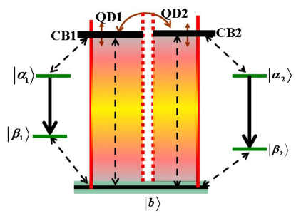
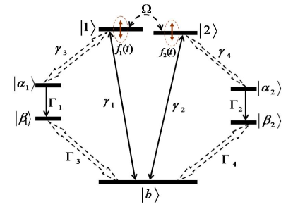
Figure 1: (Color online)(a) Schematic of electronic states of the DQD in both their eigenstate basis (solid lines). Solar radiation (depicted by warm-toned zones) drives transitions between the valence band (VB) and conduction band (CB) formed the photocell p-n junction. Other transitions are driven by ambient thermal phonon reservoir. Charge transfer to the left/right lead (denoted by states $|\alpha_{1}\rangle$ and $|\alpha_{2}\rangle$) are illustrated by dashed double-headed arrows. States $|\alpha_{i}\rangle$ and $|\beta_{i}\rangle$(_i=1,2) connected to loads form the output electric current. (b) Corresponding energy-level diagram of the DQD photocell model.

The discovery of intermediate band solar cell (IBSC) has made a breakthrough in the field of modern photovoltaic research1961Shockley ; 1997Luque , which was first introduced by Marti with the efficiency 63.2$\%$ exceeding the previous maximum 33$\%$ efficiency proposed by Shockley and Queisser. However, it is difficult to achieve in practical models due to manufacturing constraints. An intermediate band (IB£©can be achieved by the QDs2011Yang ; 2014Aly due to their multifunctionality such as small size and tuning the range of band. The formed IB provides easier transportation path for the carriers. At the same time, it may also promote the electrons to the conduction band (CB) increasing the overall generation rate2014Aly ; 2017Jian . This kind of structure may result in the multistep absorption process when arranging them in parallel or series to couple them either by tunneling or capacitively. Hence, double quantum dots (DQDs) have emerged as versatile and efficient scaffolds to absorb light and then convert optical energy into other useful forms of energy. The wave functions of closely spaced QDs get coupled and form minibands. These minibands exhibit new optoelectronics properties which is quite unique from the parent semiconductor materials2011Sugaya . Different from these previous work, we focus on the photovoltaic performance in a DQD photocell with spatially correlated fluctuation.

We propose a DQD system with each dot contacting its individual electron reservoir at zero temperature and zero bias in this suggested DQD photocell model, and the system interacts with ambient radiation and phonon thermal reservoirs (See Fig.1 (a)). In this DQD photocell model (designated as QD1 and QD2 in Fig.1 (a), the level $|b\rangle$ represents the valence band (VB), while levels $|1\rangle$ and $|2\rangle$ represent the conduction bands (CB1 and CB2). Thermal solar photons drive $|b\rangle$ $\leftrightarrow$ $|i\rangle$ transitions and have average occupation numbers $n_{i}(\frac{E_{ib}}{K_{B}T_{s}})$=$[exp(\frac{E_{ib}}{K_{B}T_{s}})-1]^{-1}$ with the energy gap $E_{ib}$(_i=1,2). At temperature $T_{a}$, low-energy transitions $|i\rangle$ $\leftrightarrow$ $|\alpha_{i}$ and $|\beta_{i}\rangle$ $\leftrightarrow$ $|b\rangle_{(i=1,2)}$ are driven by ambient thermal phonons. The corresponding phonon occupation numbers are $n_{3,4}={[exp(\frac{E_{i\alpha_{i}}}{K_{B}T_{a}})-1]}^{-1}$ and $n_{5,6}={[exp(\frac{E_{\beta_{i}b}}{K_{B}T_{a}})-1]}^{-1}$ for each. The electric charges were then transferred to the external loads through the transitions $|\alpha_{i}\rangle$ $\leftrightarrow$ $|\beta_{i}\rangle$.

Unlike the earlier DQD photocell modelZHONG2021104094 ; ZHONG2021104503 , the quantum fluctuations coupling to the CBs (corresponding to the levels $|1\rangle$ and $|2\rangle$ in Fig.1 (b)) will be examined due to its interaction with the surrounding environment. In this suggested photocell model, we will investigate spatially correlated stochastic noise processes and explain how the spatial correlation influences charge transfer. As a result, the total Hamiltonian of the DQD photovoltaic model may be stated as (For convenience, we set $\hbar=1$),

$$\hat{H_{T}}=\hat{H}_{s}+\hat{H}_{P}+\hat{H}_{s-P},$$ (1)

Without loss of generality, the DQD system has three states: the left dot occupied state $|1\rangle$, the corresponding right one $|2\rangle$, and the ground state $|b\rangle$ with both dots empty owing to the strong Coulomb repulsion limit(see in Fig.1(b))RevModPhys.75.1 . Hence, the Hamiltonian $\hat{H}_{s}$ in Eq.(1) describes these states with an extra electron in the left or right dot (i.e. in the CB states $|1\rangle$ or $|2\rangle$ ) and it contains the following physical elements,

$$\hat{H}_{s}=\hat{H}_{D}+\hat{H}_{L}+\hat{H}_{L-D},$$ (2)

in which $\hat{H}_{D}$ depicts the Hamiltonian of the DQD system with quantum fluctuation taken into account,

$$\hat{H}_{D}=\frac{\varepsilon}{2}\hat{\sigma}_{z}+\Omega\hat{\sigma}_{x}+\sum_{i=1,2}f_{i}(t)\hat{d}_{i}^{{\dagger}}\hat{d}_{i},$$ (3)

In the first term of the above Eq.(3), $\varepsilon$ describes the electrostatic energy difference between the two CB states, and the Pauli matrix is defined asRevModPhys.75.1 $\hat{\sigma}_{z}$ = $\hat{d}_{1}^{{\dagger}}\hat{d}_{1}$ - $\hat{d}_{2}^{{\dagger}}\hat{d}_{2}$ with the subspace of states $\hat{d}_{i}^{{\dagger}}$ ($\hat{d}_{i}$)_(i=1,2) representing the creation (annihilation ) operators and an electron in the left or right quantum dot, respectively. The second term in above equation depicts the tunnel effect of an electron between the two dots with $\Omega$ being the tunnel matrix element of an electron, and with Pauli operator $\hat{\sigma}_{x}$ = $\hat{d}_{1}^{{\dagger}}$$\hat{d}_{2}$ + $\hat{d}_{2}^{{\dagger}}$$\hat{d}_{1}$. If a bias DC voltage is applied to this DQD system, the two eigenstates will be splitted by $\omega$: $\hbar\omega=\sqrt{\varepsilon^{2}+\Omega^{2}}$RevModPhys.75.1 . The last item in Eq.(3) describes the spatially correlated fluctuation coupling to the two CB states owing to their interactions with the ambient environment. $f_{i}(t)$ is the fluctuating frequency on the CB states (corresponding to the levels $|1\rangle$ and $|2\rangle$ in Fig.1(b)) and is considered as a stochastic process with the average of frequency fluctuation $\langle f_{i}(t)\rangle$= 0 for each state. In this model, we will consider the fluctuation generated by the spatially correlated stochastic noise, and show what impact it will have and how to optimize the parameters of the DQD system in different ambient environment to control quantum photovoltaic properties. Therefore, for the sake of convenience, the correlation function $\langle f_{i}(0)f_{j}(t)\rangle_{(i,j=1,2)}$ is described in a exponential decay processPhysRevE.83.011906 ; npjUchiyama2018 as follows,

$$\langle f_{i}(0)f_{j}(t)\rangle_{(i,j=1,2)}=kA^{2}exp[-\frac{t}{\tau_{ij}}],$$ (4)

where $k$ is defined over the range by $-1\leq$ k $\leq 1$, its positive and negative values represent the noise with spatial or anti-spatial correlations. The extremal value $-1$ ($+1$) corresponds to perfectly anti-correlated (correlated) noise, respectively. $A$ describes the amplitude of quantum fluctuation, and $\tau_{1,2}$ is the correlation time of the fluctuation. Therefore, insights into the spatio-correlation and intensity of quantum fluctuations will be measured by the two mentioned parameters for the optimizing charge transfer and output efficiency in this DQD photovoltaic model,

In Eq.(2), $\hat{H}_{L}$ depicts the Hamiltonian of the external electrodes attached to the DQD system, the two eletrodes are modeled as collection of noninteracting electron with energy $\hbar\omega_{ik}$ and momentum $k$ in the ith (i=1,2) electrode as follows,

$$\hat{H}_{L}=\sum_{i=1,2}\sum_{k}\omega_{ik}\hat{a}_{ik}^{{\dagger}}\hat{a}_{ik},$$ (5)

in which $\hat{a}_{ik}^{{\dagger}}$ ($\hat{a}_{ik}$) depicts the creation (annihilation) operator for an electron with momentum $k$ in the ith (i=1,2) electrode. By making the rotating wave approximation approximation and with the Weisskopf-Wigner theoryZhao2019 , the Hamiltonian between the dot i and lead i(i=1,2) with the corresponding coupling constant $g_{ik}$ in Eq.(2) can be given as,

$$\hat{H}_{L-D}=\sum_{i=1,2}\sum_{k}g_{ik}\hat{d}_{ik}^{{\dagger}}\hat{a}_{ik}+H.c,$$ (6)

where $H.c$ denotes the Hermite conjugate of the previous parts in Eq.(6). In Eq.(1), the ambient environment’s Hamiltonian is written as $\hat{H}_{P}=\sum_{q}\omega_{q}\hat{b}_{q}^{{\dagger}}\hat{b}_{q}$ with its q-th noninteracting photon mode frequency $\omega_{q}$. The interaction between the DQD photovoltaic system and photon degrees of freedom, $\hat{H}_{s-P}$ in the Eq.(1) is described by the Hamiltonian Wertnik2018Optimizing with the corresponding coupling strength $\lambda_{q}$ as follows,

$$\hat{H}_{s-P}=\hat{\sigma}_{x}\sum_{q}\lambda_{q}(\hat{b}_{q}^{{\dagger}}+\hat{b}_{q}),$$ (7)

In the current work, we devote to the influence generated by the quantum fluctuations which is the fundamental difference with the previous DQD photovoltaic modelZHONG2021104094 ; PhysRevB.87.035429 ; ZHONG2021104503 . In this DQD photovoltaic model, utilizing the Lindblad-like master equation, we analytically find that there is a decay response both to the dynamics of charge transfer and delivery efficiency, and the anti-spatial correlation fluctuation in a hotter thermal ambient environment brings out the damped photovoltaic properties owing to the damaged condition for noise-induced coherence. Comparing with the photovoltaic power enhanced by Fano-induced coherencePhysRevA.84.053818 , this work will reveal some different physical regimes on the efficient photovoltaic properties due to the quantum coherence deteriorated by the quantum fluctuations.

III Dynamics behavior of the photovoltaic DQD cell

In the Schr$\ddot{o}$dinger picture the Born-Markov second order master equation takes the form,

$$\frac{d\hat{\rho}_{s}}{dt}=-i[\hat{H}_{s},\hat{\rho}_{s}]-\int^{\infty}_{0}d\tau\langle[\hat{H}_{s-P}(t),[\hat{H}_{s-P}(\tau),\hat{\rho}_{s}(t)\bigotimes\hat{\rho}_{P}(t_{0})]]\rangle_{\hat{H}_{P}},$$ (8)

where $\hat{\alpha}(\tau)$=$\exp[\frac{i}{\hbar}\hat{H}_{s}t]\hat{\alpha}(t)\exp[-\frac{i}{\hbar}\hat{H}_{s}t]$ is an operator $\hat{\alpha}$ at time $\tau$ in the interaction picture. And the symbol “$\langle\cdots\rangle_{\hat{H}_{P}}$” denotes the trace operation on photons reservoir. Utilizing the second order perturbation methodQinA2016 ; ZHONG2021104503 , the dynamics of electronic system can be described by the following Lindblad-like master equation:

$$\frac{d\hat{\rho}_{s}}{dt}=-i[\hat{H}_{s},\hat{\rho}_{s}]+\hat{L}\hat{\rho}_{s},$$ (9)

The first term on the right-hand side of Eq. (9) describes the unitary evolution of the DQD system and the second term accounts for the dissipative processes, and in which the superoperator $\hat{L}\hat{\rho}_{s}$ can be decomposed by,

$$\hat{L}\hat{\rho}_{s}=\hat{L_{h}}\hat{\rho}_{s}+\hat{L_{c(1)}}\hat{\rho}_{s}+\hat{L_{c(2)}}\hat{\rho}_{s}+\hat{L_{rel}}\hat{\rho}_{s},$$ (10)

in which $\hat{L_{h}}\hat{\rho}_{s},\hat{L_{c(1)}}\hat{\rho}_{s},\hat{L_{c(2)}}\hat{\rho}_{s},\hat{L_{rel}}\hat{\rho}_{s}$ are the superoperators related to the different dissipative processes between the DQD photovoltaic system and ambient photon (or phonon) reservoirs. As shown in Fig.1 (b), we assume that thermal solar photons are directed onto this DQD system and the solar photons are absorbed or radiated between the levels $|1\rangle$ ($|2\rangle$) and $|b\rangle$ at the rate $\gamma_{i}$. Hence, superoperator $\hat{L_{h}}\hat{\rho}_{s}$ describes transition process with the following expression,

$$\hat{L_{h}}\hat{\rho}_{s}=\sum_{i=1,2}\frac{\gamma_{i}}{2}[(n_{i}+1)\mathcal{D}[\hat{\sigma}_{bi}]\hat{\rho}_{s}+n_{i}\mathcal{D}[\hat{\sigma}_{bi}^{{\dagger}}]\hat{\rho}_{s}],$$ (11)

where $\hat{\sigma}_{bi}=|b\rangle\langle i|$ (i=1,2). Moreover, $n_{i}=[exp(x)-1]^{-1}$ is the average number of solar photons, $x=\frac{E_{i}b}{K_{B}T_{s}}_{(i=1,2)}$ with $T_{s}$, $E_{ib}$ being the solar’s temperature and corresponding gap energy, respectively. The specific expression of the symbol $\mathcal{D}$ acting on any operator $\hat{A}$ is defined as $\mathcal{D}[\,\hat{A}\,]\hat{\rho}=2\hat{A}\hat{\rho}\hat{A}^{{\dagger}}-\hat{\rho}\hat{A}^{{\dagger}}\hat{A}-\hat{A}^{{\dagger}}\hat{A}\hat{\rho}$. The dissipative transitions $|i_{(i=1,2)}\rangle$ $\leftrightarrow$ $|\alpha_{i(i=1,2)}\rangle$ is depicted by the super-operator $\hat{L_{c(1)}}\hat{\rho}_{s}$ with the following formula,

$$\hat{L_{c(1)}}\hat{\rho}_{s}=\frac{\gamma_{3,4}}{2}[(n_{3,4}+1)\mathcal{D}[\hat{\sigma}_{\alpha_{i}i}]\hat{\rho}_{s}+n_{3,4}\mathcal{D}[\hat{\sigma}_{\alpha_{i}i}^{{\dagger}}]\hat{\rho}_{s}],$$ (12)

where $\gamma_{3,4}$ are the spontaneous decay rates corresponding to the transitions $|1\rangle$ $\leftrightarrow$ $|\alpha_{1}\rangle$ and $|2\rangle$ $\leftrightarrow$ $|\alpha_{2}\rangle$, respectively. And these transitions coupled to the ambient environment have the related phonon numbers $n_{3,4}=[exp(y)-1]^{-1}$, $y=\frac{E_{i\alpha_{i}}}{K_{B}T_{a}}_{(i=1,2)}$ with the ambient temperature $T_{a}$ and the energy difference $E_{i\alpha_{i}}$. The Pauli operator $\hat{\sigma}_{\alpha_{i}i}$ is defined as $\hat{\sigma}_{\alpha_{i}i}=|\alpha_{i}\rangle\langle i|$ (i=1,2). Similarly,the dissipative process in the transition between $|\beta_{i(i=1,2)}\rangle$ $\leftrightarrow$ $|b\rangle$ can be written as

$$\hat{L_{c(2)}}\hat{\rho}_{s}=\frac{\Gamma_{3,4}}{2}[(n_{5,6}+1)\mathcal{D}[\hat{\sigma}_{\beta_{i}b}]\hat{\rho}_{s}+n_{5,6}\mathcal{D}[\hat{\sigma}_{\beta_{i}b}^{{\dagger}}]\hat{\rho}_{s}],$$ (13)

In these dissipation processes, $\Gamma_{3,4}$ are the spontaneous decay rate corresponding to the transitions $|\beta_{1}\rangle$ $\leftrightarrow$ $|b\rangle$ and $|\beta_{2}\rangle$ $\leftrightarrow$ $|b\rangle$(see in the fig.1(b)), respectively. And the phonons numbers induced by the interference between these transitions are $n_{5,6}={[exp(z)-1]}^{-1}$ with $z=\frac{E_{\beta_{i}b}}{K_{B}T_{a}}$ and $T_{a}$ being the ambient temperature, the energy difference $E_{\beta_{i}b}$_(i=1,2). The Pauli operator $\hat{\sigma}_{\beta_{i}i}$ in Eq.(13) is defined as $\hat{\sigma}_{\beta_{i}i}=|\beta_{i}\rangle\langle b|_{(i=1,2)}$ .

In this proposed DQD photovoltaic model, it contains two output terminals which can be directly connected to the external circuit. The photovoltaic currents are proportional to the relaxation rates $\Gamma_{1,2}$ via the dissipation processes $|\alpha_{i}\rangle$ $\leftrightarrow$ $|\beta_{i}\rangle$, which is defined as follows,

$$\hat{L_{rel}}\hat{\rho}_{s}=\sum_{i=1,2}\frac{\Gamma_{i}}{2}(|\beta_{i}\rangle\langle\alpha_{i}|\hat{\rho}|\alpha_{i}\rangle\langle\beta_{i}|-|\alpha_{i}\rangle\langle\alpha_{i}|\hat{\rho}-\hat{\rho}|\alpha_{i}\rangle\langle\alpha_{i}|),$$ (14)

Consequently, $|\alpha_{1}\rangle$ and $|\alpha_{2}\rangle$ are acted as charge separation states in this DQD photocell model. When the electrons are released from $|\alpha_{1}\rangle$ to $|\beta_{1}\rangle$ or from the second way $|\alpha_{2}\rangle$ to $|\beta_{2}\rangle$, the DQD is positively charged. The electrons are brought back to the neutral ground state $|b\rangle$ from $|\beta_{1}\rangle$ or $|\beta_{2}\rangle$, which completes a closed loop. With this knowledge, this photovoltaic model is similar to the parallel circuit in classical electromagnetism. Thus, the collective currents can be defined by,

$$j=e\sum_{i=1,2}\Gamma_{i}{\rho}_{\alpha_{i}\alpha_{i}},$$ (15)

Considering the Boltzmann distribution on the upper and lower levels $|\alpha_{i}\rangle$ and $|\beta_{i}\rangle$ with the populations on the two levels being as follows,

$$\rho_{\alpha_{i}\alpha_{i}}= exp(-\frac{E_{\alpha_{i}}-\mu_{\alpha_{i}}}{k_{B}T_{a}}),$$ (16)

$$\rho_{\beta_{i}\beta_{i}}= exp(-\frac{E_{\beta_{i}}-\mu_{\beta_{i}}}{k_{B}T_{a}}),$$ (17)

The total output voltage can be defined by the difference of the chemical potentials $\mu_{\alpha_{i}}$ and $\mu_{\beta_{i}}$ as follows,

$$eV=\sum_{i=1,2}(E_{\alpha_{i}}-E_{\beta_{i}}+K_{B}T_{a}\ln\frac{\rho_{\alpha_{i}\alpha_{i}}}{\rho}_{\beta_{i}\beta_{i}}),$$ (18)

Utilizing the definitions of the current and the voltage mentioned in Eq.(15) and Eq.(18), we can intuitively deduce the output power of this DQD photovoltaic model with the classic definition $P=jV$. Considering that incident solar photons are directed on the DQD photovoltaic system, the absorbed solar photons irrigate the DQD photovoltaic system with the input energy $P_{s}$. Therefore, the delivery efficiency of this photovoltaic system can be expressed as,

$$\eta=\frac{P}{Ps},$$ (19)

Unlike the traditional processing methodPhysRevB.87.035429 ; PhysRevA.84.053818 , we are not concerned with quantum coherence itself, but rather with the influence of quantum fluctuations on photovoltaic characteristics, and we attempt to fundamentally reveal the physical mechanism that affects quantum interference. As a result, the influence generated by external environments is reduced during the interaction with the external environment under the Weisskopf-Wigner approximation1974On , and the reduced matrix elements corresponding to Eg.(9) are listed as follows:

$$\dot{\rho}_{11}= -i\Omega(\rho_{21}-\rho_{12})-i\gamma_{3}(\rho_{\alpha_{1}1}-\rho_{1\alpha_{1}})-\gamma_{3}[(n_{3}+1)\rho_{11}-n_{3}\rho_{\alpha_{1}\alpha_{1}}]$$

$$-\gamma_{1}[(n_{1}+1)\rho_{11}-n_{1}\rho_{bb}],$$

$$\dot{\rho}_{22}= i\Omega(\rho_{21}-\rho_{12})-i\gamma_{4}(\rho_{\alpha_{2}2}-\rho_{2\alpha_{2}})-\gamma_{4}[(n_{4}+1)\rho_{22}-n_{4}\rho_{\alpha_{2}\alpha_{2}}]$$

$$-\gamma_{2}[(n_{2}+1)\rho_{22}-n_{2}\rho_{bb}],$$

$$\dot{\rho}_{12}= -i\varepsilon\rho_{12}-i\Omega(\rho_{22}-\rho_{11})-i\rho_{12}(f_{1}(t)-f_{2}(t))-\frac{\rho_{12}}{2}[\gamma_{1}(n_{1}+1)$$

$$+\gamma_{2}(n_{2}+1)+\gamma_{3}(n_{3}+1)+\gamma_{4}(n_{4}+1)],$$

$$\dot{\rho}_{21}= i\varepsilon\rho_{21}+i\Omega(\rho_{22}-\rho_{11})+i\rho_{21}(f_{1}(t)-f_{2}(t))-\frac{\rho_{21}}{2}[\gamma_{1}(n_{1}+1)$$

$$+\gamma_{2}(n_{2}+1)+\gamma_{3}(n_{3}+1)+\gamma_{4}(n_{4}+1)],$$

$$\dot{\rho}_{\alpha_{1}\alpha_{1}}= i\gamma_{3}(\rho_{\alpha_{1}1}-\rho_{1\alpha_{1}})+\gamma_{3}[(n_{3}+1)\rho_{11}-n_{3}\rho_{\alpha_{1}\alpha_{1}}]-\Gamma_{1}\rho_{\alpha_{1}\alpha_{1}},$$

$$\dot{\rho}_{\alpha_{2}\alpha_{2}}= i\gamma_{4}(\rho_{\alpha_{2}2}-\rho_{2\alpha_{2}})+\gamma_{4}[(n_{4}+1)\rho_{22}-n_{4}\rho_{\alpha_{2}\alpha_{2}}]-\Gamma_{2}\rho_{\alpha_{2}\alpha_{2}},$$

$$\dot{\rho}_{\beta_{1}\beta_{1}}= \Gamma_{1}\rho_{\alpha_{1}\alpha_{1}}-\Gamma_{3}[(n_{5}+1)\rho_{\beta_{1}\beta_{1}}-n_{5}\rho_{bb}],$$

$$\dot{\rho}_{\beta_{2}\beta_{2}}= \Gamma_{2}\rho_{\alpha_{2}\alpha_{2}}-\Gamma_{4}[(n_{6}+1)\rho_{\beta_{2}\beta_{2}}-n_{6}\rho_{bb}],$$

$$\dot{\rho}_{1\alpha_{1}}= -i\gamma_{3}(\rho_{\alpha_{1}\alpha_{1}}-\rho_{11})+i(\omega_{1}-\frac{\varepsilon}{2}){\rho}_{1\alpha_{1}}-if_{1}(t){\rho}_{1\alpha_{1}}$$

$$-\frac{\rho_{1\alpha_{1}}}{2}[\gamma_{1}(n_{1}+1)+\gamma_{3}(2n_{3}+1)+\Gamma_{1}],$$

$$\dot{\rho}_{\alpha_{1}1}= i\gamma_{3}(\rho_{\alpha_{1}\alpha_{1}}-\rho_{11})-i(\omega_{1}-\frac{\varepsilon}{2}){\rho}_{\alpha_{1}1}+if_{1}(t){\rho}_{\alpha_{1}1}$$

$$-\frac{\rho_{\alpha_{1}1}}{2}[\gamma_{1}(n_{1}+1)+\gamma_{3}(2n_{3}+1)+\Gamma_{1}],$$

$$\dot{\rho}_{2\alpha_{2}}= -i\gamma_{4}(\rho_{\alpha_{2}\alpha_{2}}-\rho_{22})+i(\omega_{2}+\frac{\varepsilon}{2}){\rho}_{2\alpha_{2}}-if_{2}(t){\rho}_{2\alpha_{2}}$$

$$-\frac{\rho_{2\alpha_{2}}}{2}[\gamma_{2}(n_{2}+1)+\gamma_{4}(2n_{4}+1)+\Gamma_{2}],$$

$$\dot{\rho}_{\alpha_{2}2}= i\gamma_{4}(\rho_{\alpha_{2}\alpha_{2}}-\rho_{22})-i(\omega_{2}+\frac{\varepsilon}{2}){\rho}_{\alpha_{2}2}+if_{2}(t){\rho}_{\alpha_{2}2}$$

$$-\frac{\rho_{\alpha_{2}2}}{2}[\gamma_{2}(n_{2}+1)+\gamma_{4}(2n_{4}+1)+\Gamma_{2}].$$

IV Delayed response to the photovoltaic properties due to the spatially correlated fluctuation

To verify the photovoltaic properties in this DQD photocell model, we assess the charge transfer dynamics with some selected parameters, such as $E_{i}-E_{\alpha_{i}}$=$E_{\beta_{i}}-E_{b}=0.005eV$PhysRevA.84.053818 , $\gamma_{1}$ =$6.28\gamma$, $\gamma_{2}$ =$1.18\gamma$, $\gamma_{3}$=$\gamma_{4}$=$4.02\gamma$, $\Gamma_{1}$=$3.58\gamma$, $\Gamma_{2}$=$3.15\gamma$, $\Gamma_{3}$=$\Gamma_{4}$=$0.04\gamma$ with $\gamma$=$10^{-8}Hz$. Considering the fact that a small number of solar photons are absorbed at per unit time as well as weak-coupling between the DQD system and ambient environment, the photons with $\hbar\omega_{1}$=1.64 eV, $\hbar\omega_{2}$=1.6 eV are absorbed in the generated photovoltaic current process, and the numbers of photoelectron are set as $n_{1}$=30 and $n_{2}$=15 populated on the CB states $|1\rangle$ and $|2\rangle$, respectively. The correlation time of the fluctuation between two CBs, $\tau_{12}$= 2.5 femtosecond. For the sake of applicability, we do not use gap energy as a controlling parameter, but utilize interdot gap energy difference $\varepsilon$ to revaluate the photovoltaic properties in our subsequent discussion.

At the ambient temperature is close to room temperature, i.e., $T_{a}$=0.026$eV$, the interdot tunneling coefficient $\Omega$=0.03, gap energy difference $\varepsilon$=0.04$eV$, $k$=0.1 in Fig.2(a1) while $\Omega$= 0.0025, $\varepsilon$=0.01$eV$, fluctuation amplitude $A$=0.9 in Fig.2(a2) are utilized, respectively. We numerically solve the Eqs.(III) and plot the evolution of output current with different spatially correlated fluctuation amplitudes $A$, and output efficiency with different spatio-correlation robustness $k$ in Fig.2(a1) and (a2), respectively. In order to highlight the role of spatially correlated fluctuations in photovoltaic performance, other parameters, such as the self-structure and other performance parameters, ambient temperatures are not concluded in Fig.2.

The dashed lines in Fig.2 (a1) and (a2) show a striking delayed response to the photovoltaic behavior, illustrating the prolonging peak times with the increments of $A$ and $k$ , respectively. The curves in Fig.2 (a1) show the delayed response as the spatially correlated fluctuation amplitudes $A$ increase, whereas the curves in Fig.2 (a2) show the increasing spatial correlation robustness $k$. Furthermore, we can see that the parameters $k$ and $k$ have no effect on the peaks and final steady values. However, we believe that the delayed response will affect the physical behavior of charge transfer and, as a result, the photovoltaic performance under various operating conditions. With this in mind, we continue to investigate the regulation influence on delayed response via some structural parameters, with the goal of clarifying the role of delayed response in this DQD photovoltaic model.

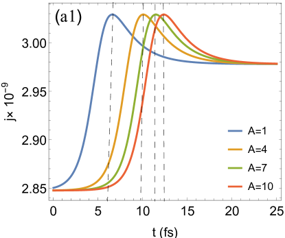
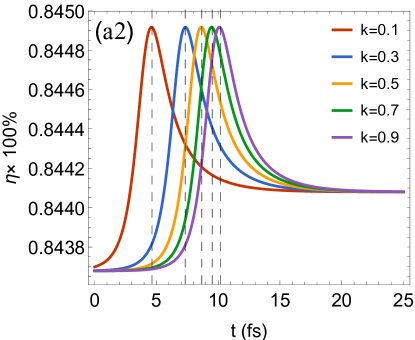
Figure 2: (Color online) Dynamics of the photovoltaic behavior influenced by spatially correlated fluctuations. (a1) Evolution of output current with different spatially correlated fluctuation amplitudes $A$, (a2) Evolution of delivery efficiency under different spatial correlation robustness $k$.

V Regulating strategies for delayed response

V.1 Delayed response regulated by the gap differences

So far, the delayed response caused by spatially correlated fluctuations in the DQD photovoltaic cell has not been reported. We hypothesize that the delayed response caused by spatially correlated fluctuations is inhibited by a physical regime generated by the DQD itself. In order to better illustrate the underlying physical mechanisms, the spatial correlation robustness and fluctuation amplitudes are set to $k$=0.3, $A$=0.9, respectively, in the following discussion; all other parameters are the same as in Fig.2.

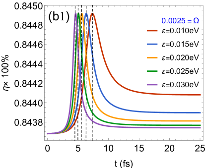
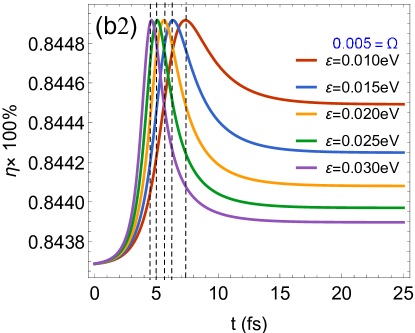
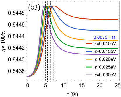
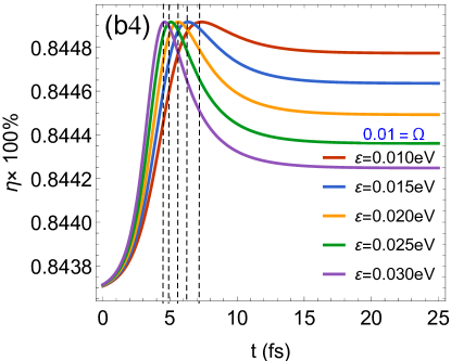
Figure 3: (Color online) Evolution of the output photovoltaic efficiency controlled by gap energy difference with different inter-dot tunneling coefficients (b1) $\Omega$$=$0.0025, (b2) $\Omega$$=$0.005, (b3) $\Omega$$=$0.0075, (b4) $\Omega$$=$0.01.

The curves in Fig.3 back up our theory about the underlying physical regime. The times corresponding to the peaks, as well as the final stable output efficiencies, decrease as the interdot gap energy difference $\varepsilon$ increases, as shown in Fig.3 (b1). In addition to these, two noteworthy conclusions emerge from a comparison of the curves in Fig.3 (b1) with (b2), (b3) and (b4). The peak efficiencies and delayed times, as shown by the peaks and their corresponding times, hardly change with increments of $\Omega$. The other is that stable efficiencies ascend in parallel with $\Omega$, as shown by the horizontal lines in Fig.3 from (b1) to (b4).

These results show that increasing the gap difference $\varepsilon$ can reduce the delayed response as well as the final steady output efficiencies, indicating that $\varepsilon$ describing the structure of the DQD may be an efficient approach to inhibiting the delayed response generated by the spatially correlated fluctuation. However, we hypothesize that the charge transfer between two adjacent quantum dots was reduced due to the increasing gap difference $\varepsilon$, resulting in a decrease in output efficiency, which could be the physical regime for the descending horizontal lines in Fig.3. Meanwhile, the tunneling effect can reinforce charge transfer, but the spatially correlated fluctuation is not involved, resulting in more photoinduced charges being transported in the end while the time delayed response is almost unaffected. The tunneling coefficient $\Omega$ is well known to describe the energy transfer behavior between two dots, which can be flexibly tuned by applying an external bias voltage to the two dotsRevModPhys.75.1 ; ZHAO2009 . As a result, in this proposed DQD photocell model, the applied bias voltage may be suggested to overcome the passive influence generated by the gap difference $\varepsilon$. Actually, these findings may explain why no significant quantum fluctuation effect has been observed in macroscopic DQD photovoltaic cells thus far.

V.2 Delayed response dependent the spatial or anti-spatial correlations

In Eq.(4), the spatially correlated noise parameter $k$ with its positive or negative values represents the spatially or anti-spatially correlated degree, which directly reflects the correlated behaviors of quantum fluctuations owing to the environment noise. Therefore, it is possible to find some underlying physical strategies to restrain the delayed response by vesting insight into the spatially correlated noise parameter $k$ in different thermal environments. From Eq.(4), a linear relationship can be observed between spatially correlated noise parameter $k$ and fluctuation intensity. Thus, the regulation features of noise parameter $k$ can directly reveal the physical behaviors of the spatially or anti-spatially correlated fluctuations.

To facilitate the comparison with the results achieved in Fig.3, the interdot tunneling coefficient $\Omega$ and gap difference $\varepsilon$ are set as $\Omega$$=$0.0025, $\varepsilon$=0.01 $eV$ in the upcoming discussion, and other parameters are the same to those in Fig.3. Thereupon, the dependence of output photovoltaic efficiency on different spatially correlated noise parameter $k$ is plotted in Fig.4. As the peaks of curves shown in Fig.4 (c1), the times corresponding the peak efficiencies illustrate that, the delayed response becomes more prominent and obvious with the increments of spatial correlations noise parameters $k$ at $T_{a}$$=$0.0256 $eV$. In addition to these, the peak photovoltaic efficiency slips from 84.52$\%$, 84.50$\%$, 84.48$\%$ to 84.46$\%$ when the ambient temperature increases in Fig.4 from (c1) to (c4) by 0.0256 $eV$, 0.0258 $eV$, 0.0262 $eV$ and 0.0264 $eV$, as well as their final steady values delivering efficiencies are uniform but descend with the increments of $T_{a}$.

The above results show that increasing the spatial correlations noise parameters $k$ results in a more prominent delayed response, but the DQD photovoltaic properties are diminished by the hotter thermal ambient environment. Noise-induced coherence2014Noise was shown in a decay modelScully15097 to break detailed balance and get more power out of a photocell due to noise-induced coherence against environmental decoherence. As a result, we believe that larger spatially correlated noise parameters $k$ only delayed but did not weaken noise-induced coherence. As a result, a more prominent delayed response is obtained, but peak efficiencies do not change as the spatially correlated fluctuation in the DQD photocell system increases. However, because noise-induced quantum coherence is impressionable to ambient temperaturesZhao2019 , the output photovoltaic performances decrease as ambient temperature increases.

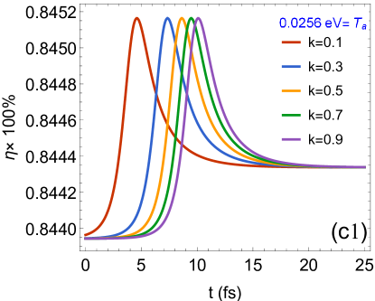
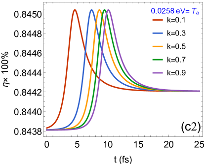
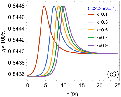
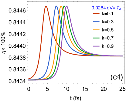
Figure 4: (Color online) Evolution of the output photovoltaic efficiency with different spatial correlated noise parameters $k$ in different thermal ambient environment. (c1) $T_{a}$$=$0.0256 $eV$, (c2) $T_{a}$$=$0.0258 $eV$, (c3) $T_{a}$$=$0.0262 $eV$, (c4) $T_{a}$$=$0.0264 $eV$.

As mentioned before, the anti-spatial correlated noise is represented by the negative values of the spatially correlated noise parameter $k$ npjUchiyama2018 . The negative property of anti-spatial correlated noise may show another physical property and bring out some different photovoltaic characteristics in this photocell model, which is our another concern. Different from the previous results with the spatial correlated fluctuation, a completely different linetype distributions, the hysteresis loop-style graph is obtained owing to the anti-spatially correlated noise in Fig.5. As the curves shown in Fig.5, the steady peak efficiencies decrease with the ambient temperature, which still suggests a negative effect on the steady output efficiencies due to $T_{a}$, as coincides with those shown in Fig.4. Not only that, but the final steady peak efficiencies do not vary with the anti-spatial correlated noise parameters $k$, as well as the anti-spatial correlated noise parameters $k$ hardly exert influence over the delayed response (see the curves in Fig.5(d1)). What’s more, in the evolutionary process to the stable peaks, the photovoltaic efficiencies decrease with the increments of $k$ from -0.1, 0.3, 0.5, 0.7 to -1.0, i. e., the larger anti-spatial correlated noise parameters $k$, the lower output photovoltaic efficiency. So, results infer the output photovoltaic efficiency can be suppressed by the anti-spatial correlated noise parameters $k$.

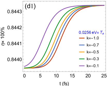
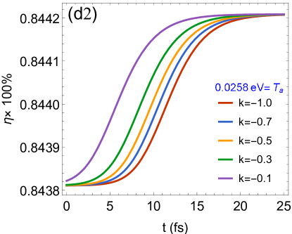
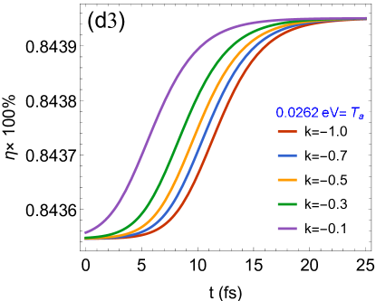
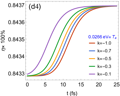
Figure 5: (Color online) Evolution of photoelectric conversion efficiency with different anti-spatial correlated noise parameters $k$ at different ambient temperatures. (d1) $T_{a}$$=$0.0256 $eV$, (d2) $T_{a}$$=$0.0258 $eV$, (d3) $T_{a}$$=$0.0262 $eV$, (d4) $T_{a}$$=$0.0266 $eV$.

Let’s take a closer look at the physical implications implied by Fig.5. When we compare the roles of spatial and anti-spatial correlated noise in Fig.4 and Fig.5, we find that the spatially correlated noise causes a large time delay, but it has no effect on the output photovoltaic efficiency. However, anti-spatial correlated noise has no effect on peak photovoltaic efficiency, whereas in its evolutionary process, the stronger the anti-spatial correlated noise, the lower the output photovoltaic efficiency. Based on previous research on noise-induced coherenceScully15097 ; 2014Noise , we believe that the delayed photovoltaic properties are due to the generative process of noise-induced coherence being delayed by spatially correlated noise, whereas the reduced photovoltaic efficiency is due to the ambient temperature for noise-induced coherence being deteriorated by anti-spatial correlated noise. Furthermore, the hotter thermal ambient environment interferes with the generation of noise-induced coherence. As a result, the photoelectric conversion efficiency decreases as ambient temperature rises.

VI Conclusions and remarks

We introduce spatially correlated fluctuations to the two CBs in this proposed QDQ photovoltaic model and focus on the physical implications rather than the photovoltaic model itself. In this DQD photovoltaic model, the delayed response are demonstrated to the charge transfer and the process of ascending to the peak photovoltaic efficiency, while a natural adjustment feature was also verified on the delayed response in this DQD photocell model. Further investigation reveals that the spatial correlated noise generates the delayed response, and the anti-spatial correlated noise can reduce the output photovoltaic efficiency, which is not the same as those in Ref.PhysRevE.78.050902 . Quantum coherence, on the other hand, has been shown to improve transport processes in both photosynthesis and photocellshttps://doi.org/10.1002/slct.201803554 ; doi:10.1021/acs.jpcb.0c10719 ; 2019Intervalley . Based on these, we hypothesize that the physical mechanism underlying the aforementioned conclusions is quantum coherence controlled by spatially correlated fluctuation. When the noise-induced coherence process is delayed by spatially correlated fluctuation, the output photovoltaic properties are inevitably delayed. While the anti-spatially correlated noise destroyed the condition for noise-induced coherence, the photovoltaic properties were reduced. Furthermore, the thermal ambient temperature degrades the environment for the generation of noise-induced coherence, which is one of the factors that reduces photovoltaic performance in this DQD photovoltaic model.

We’d like to make a few comments before we wrap up this paper. First, the spatially correlated fluctuations were imposed on the two CBs in our current work. However, the external load, i.e. the acceptor, may experience similar quantum fluctuations, and our work is unrelated to the results that the efficiencies are affected by acceptor fluctuations. However, the physical mechanism underlying such spatially correlated fluctuations and how it influences quantum photovoltaic properties remain unknown. On the other hand, because of the direct improvement in photovoltaic performance, revealing the relationship between spatially correlated fluctuations and long-lived coherence is a very important topic in DQD photovoltaic systems. As a result, we will broaden our current research to include DQD photovoltaic systems and the relationship between spatially correlated fluctuations and long-lived coherence. We believe that these relationships will help us understand the implicit physical significance of charge transfer and provide new insights into some fundamental problems in DQD photovoltaic systems.

Competing Interests

The authors declare no competing financial or non-financial interests. This article does not contain any studies with human participants or animals performed by any of the authors. Informed consent was obtained from all individual participants included in the study.

Data Availability

This manuscript has associated data in a data repository. [Authors¡¯ comment: All data included in this manuscript are available upon reasonable request by contacting with the corresponding author.]

Author contributions

S. C. Zhao conceived the idea. S. N. Zhu performed the numerical computations and wrote the draft, and S. C. Zhao did the analysis and revised the paper. L. X. Xu and L. J. Chen participated in part of the discussion.

References

- (1) G. S. Engel, T. R. Calhoun, E. L. Read, T. K. Ahn, T. Mancal, Y. C. Cheng, R. E. Blankenship, and G. R. Fleming. Evidence for wavelike energy transfer through quantum coherence in photosynthetic systems. Nature, 446(7137):782–786, 2007.
- (2) J. Wu, F. Liu, Y. Shen, J. Cao, and R. J. Silbey. Efficient energy transfer in light-harvesting systems, i: optimal temperature, reorganization energy and spatial¨ctemporal correlations. New Journal of Physics, 12:105012, 2010.
- (3) D. Mccutcheon and A. Nazir. Coherent and incoherent dynamics in excitonic energy transfer: Correlated fluctuations and off-resonance effects. Physics, 83(16), 2010.
- (4) G. Panitchayangkoon, D. Hayes, K. A. Fransted, J. R. Caram, and G. S. Engel. Long-lived quantum coherence in photosynthetic complexes at physiological temperature. Proceedings of the National Academy of Sciences, 107(29):12766–12770, 2010.
- (5) E. Collini, C. Y. Wong, K. E. Wilk, Pmg Curmi, P. Brumer, and G. D. Scholes. Coherently wired light-harvesting in photosynthetic marine algae at ambient temperature. Nature, 463(7281):644–7, 2010.
- (6) J. Seibt and Tnu Pullerits. Combined treatment of relaxation and fluctuation dynamics in the calculation of two-dimensional electronic spectra. Journal of Chemical Physics, 141(11):114106, 2014.
- (7) J. Lim, D. J. Ing, J. Rosskopf, J. Jeske, J. H. Cole, S. F. Huelga, and M. B. Plenio. Signatures of spatially correlated noise and non-secular effects in two-dimensional electronic spectroscopy. Journal of Chemical Physics, 146(2):024109, 2017.
- (8) D. Singh and S. Dasgupta. Role of initial coherence in excitation energy transfer in fenna-matthews-olson complex. Chemistry Select, (4):2703, 2019.
- (9) D. Singh. Coherent speedup of excitation energy transfer in pc645. The Journal of Physical Chemistry B, 125:557, 2021.
- (10) Z. G. Yu, M. A. Berding, and Haobin Wang. Spatially correlated fluctuations and coherence dynamics in photosynthesis. Phys. Rev. E, 78:050902, 2008.
- (11) R. Dutta and B. Bagchi. Quantum coherence and its signatures in extended quantum systems. J. Phys. Chem. B, 124:4551, 2020.
- (12) D. Mccutcheon and A. Nazir. Coherent and incoherent dynamics in excitonic energy transfer: Correlated fluctuations and off-resonance effects. Phys. Rev. B, 83:165101, 2011.
- (13) F. Fassioli, A. Nazir, and A. Olaya-Castro. Quantum state tuning of energy transfer in a correlated environment. Journal of Physical Chemistry Letters, 1(14):2139–2143, 2010.
- (14) D. Abramavicius and S. Mukamel. Exciton dynamics in chromophore aggregates with correlated environment fluctuations. Journal of Chemical Physics, 134:174504, 2011.
- (15) E. Hennebicq, D. Beljonne, C. Curutchet, G. D. Scholes, and R. J. Silbey. Shared-mode resonant energy transfer in the weak coupling regime. The Journal of Chemical Physics, 130(21):214505, 2009.
- (16) A. A. Svidzinsky, K. E. Dorfman, and M. O. Scully. Enhancing photovoltaic power by fano-induced coherence. Phys. Rev. A, 84:053818, 2011.
- (17) M. O. Scully, K. R. Chapin, K. E. Dorfman, M. B. Kim, and A. Svidzinsky. Quantum heat engine power can be increased by noise-induced coherence. Proceedings of the National Academy of Sciences, 108(37):15097–15100, 2011.
- (18) E. R. Bittner and C. Silva. Noise-induced quantum coherence drives photo-carrier generation dynamics at polymeric semiconductor heterojunctions. Nature Communications, 5:3119, 2014.
- (19) X. L. Xu, H. Ge, C. Gu, Y. Q. Gao, S. S. Wang, B. J. R. Thio, J. T. Hynes, X. S. Xie, and J. S. Cao. Modeling spatial correlation of dna deformation: Dna allostery in protein binding. The Journal of Physical Chemistry B, 117(42):13378–13387, 2013.
- (20) T.S. Kim and S. Hershfield. Suppression of current in transport through parallel double quantum dots. Phys. Rev. B, 63:245326, 2001.
- (21) Z. G. Yu. Fluorescent resonant energy transfer: correlated fluctuations of donor and acceptor. Journal of Chemical Physics, 127(22):221101, 2007.
- (22) S. C. Zhao and Q. X. Wu. High quantum yields generated by a multi-band quantum dot photocell. Superlattices and microstructures, 137:106329, 2020.
- (23) M. O. Scully. Quantum photocell: Using quantum coherence to reduce radiative recombination and increase efficiency. Phys. Rev. Lett., 104(20):207701, 2010.
- (24) K. E. Dorfman, D. V. Voronine, S. Mukamel, and M. O. Scully. Photosynthetic reaction center as a quantum heat engine. Proceedings of the National Academy of Sciences, 110(8):2746, 2013.
- (25) S. C. Zhao and J. Y. Chen. Enhanced quantum yields and efficiency in a quantum dot photocell modeled by a multi-level system. New Journal of Physics, 21(10):103015, 2019.
- (26) O. E. Semonin, J. M. Luther, S. Choi, H. Y. Chen, J. Gao, A. J. Nozik, and M. C. Beard. Peak external photocurrent quantum efficiency exceeding 100 via MEG in a quantum dot solar cell. Science, 334(6062):1530, 2011.
- (27) C. Wang, J. Ren, and J. S. Cao. Optimal tunneling enhances quantum photovoltaic effect in double quantum dots. New Journal of Physics, 16(4), 2013.
- (28) S. Q. Zhong, S. C. Zhao, and S. N. Zhu. Photovoltaic properties enhanced by the tunneling effect in a coupled quantum dot photocell. Results in Physics, 24:104094, 2021.
- (29) L. L. Tatarinova and M. E. Garcia. Analytical theory for the propagation of laser beams in nonlinear media. Phys. Rev. A, 76(4):538, 2007.
- (30) A. A. Belyanin, F. Capasso, V. V. Kocharovsky, Vl. V. Kocharovsky, and M. O. Scully. Infrared generation in low-dimensional semiconductor heterostructures via quantum coherence. Phys. Rev. A, 63:053803, 2001.
- (31) S. E. Harris. Electromagnetically induced transparency. Phys. Today, 50(7):36, 1997.
- (32) N. Liu, L. Langguth, T. Weiss, J. Kstel, M. Fleischhauer, T. Pfau, and H. Giessen. Plasmonic analogue of electromagnetically induced transparency at the drude damping limit. Nature Materials, 8(9):758, 2009.
- (33) L. V. Hau, S. E. Harris, Z. Dutton, and C. H. Behroozi. Light speed reduction to 17 metres per second in an ultracold atomic gas. Nature, (397):549, 1999.
- (34) W. Shockley and H. J. Queisser. Detailed balance limit of efficiency of p-n junction solar cells. Journal of Applied Physics, 32(3):510–519, 1961.
- (35) A. Luque and A. Mart¨ª. Increasing the efficiency of ideal solar cells by photon induced transitions at intermediate levels. Physical Review Letters, 78(26):5014–5017, 1997.
- (36) X. G. Yang, Y. Tao, K. F. Wang, Y. X. Gu, and Z G Wang. Intermediate-band solar cells based on inas/gaas quantum dots. Chinese Physics Letters, 28(3):38401–38403(3), 2011.
- (37) El Maaty Aly and A. Nasr. Theoretical study of one-intermediate band quantum dot solar cell. International Journal of Photoenergy, 2014(10):904104, 2014.
- (38) X. Jian, S. Liu, Y. Gao, W. Zhang, W. He, A. Mahmood, C M Subramaniyam, X. Wang, N. Mahmood, and S. Dou. Facile synthesis of three dimensional sandwiched mno2@gcs@mno2 hybrid nanostructured electrode for electrochemical capacitors. Acs Applied Materials Interfaces, page acsami.7b04416, 2017.
- (39) T. Sugaya, O. Numakami, S. Furue, H. Komaki, T. Amano, K. Matsubara, Y. Okano, and S. Niki. Tunnel current through a miniband in ingaas quantum dot superlattice solar cells. Solar Energy Materials Solar Cells, 95(10):2920–2923, 2011.
- (40) S. Q. Zhong, S. C. Zhao, and S. N. Zhu. Photovoltaic performances in a cavity-coupled double quantum dots photocell. Results in Physics, 27:104503, 2021.
- (41) W. G. van der Wiel, S. De Franceschi, J. M. Elzerman, T. Fujisawa, S. Tarucha, and L. P. Kouwenhoven. Electron transport through double quantum dots. Rev. Mod. Phys., 75:1–22, 2002.
- (42) M. Sarovar, Y. C. Cheng, and K. B. Whaley. Environmental correlation effects on excitation energy transfer in photosynthetic light harvesting. Phys. Rev. E, 83:011906, 2011.
- (43) C. Uchiyama, Munro W. J., and K. Nemoto. Environmental engineering for quantum energy transport. npj Quantum Information, 4:33, 2018.
- (44) W. Melina, C. Alex, N. Franco, and L. Neill. Optimizing co-operative multi-environment dynamics in a dark-state-enhanced photosynthetic heat engine. The Journal of chemical physics, 149(8):084112, 2018.
- (45) C. R. Xu and M. G. Vavilov. Quantum photovoltaic effect in double quantum dots. Phys. Rev. B, 87:035429, 2013.
- (46) M. Qin, H. Z. Shen, and X. X. Yi. A multi-pathway model for photosynthetic reaction center. J. Chem. Phys., 144:125103, 2016.
- (47) Y. K. Wang and I. C. Khoo. On the wigner-weisskopf approximation in quantum optics. Optics Communications, 11(4):323–326, 1974.
- (48) S. C. Zhao and Z. D Liu. Manipulative properties of asymmetric double quantum dots via laser and gate voltage. Chin. Phys. Lett., 26(7):077802, 2009.
- (49) D. Singh and S. Dasgupta. Role of coherence in excitation transfer efficiency to the reaction center in photosynthetic bacteria chlorobium tepidum. ChemistrySelect, 4(9):2703–2710, 2019.
- (50) D. Singh. Coherent speedup of excitation energy transfer in PC645. The Journal of Physical Chemistry B, 125(2):557–561, 2021.
- (51) S. M. Sadeghi and J. Z. Wu. Intervalley quantum coherence transfer and coherently-induced chiral plasmon fields in ws2-metallic nanoantenna systems. ACS Photonics, (6):2441–2449, 2019.